A Novel Ultrasonic Method to Quantify Bolt Tension

University of South FloridaScholar Commons

Graduate Theses and Dissertations Graduate School

January 2012

A Novel Ultrasonic Method to Quantify BoltTensionJairo Andres Martinez GarciaUniversity of South Florida, [email protected]

Follow this and additional works at: http://scholarcommons.usf.edu/etd

Part of the Acoustics, Dynamics, and Controls Commons, and the American Studies Commons

This Thesis is brought to you for free and open access by the Graduate School at Scholar Commons. It has been accepted for inclusion in GraduateTheses and Dissertations by an authorized administrator of Scholar Commons. For more information, please contact [email protected].

Scholar Commons CitationMartinez Garcia, Jairo Andres, "A Novel Ultrasonic Method to Quantify Bolt Tension" (2012). Graduate Theses and Dissertations.http://scholarcommons.usf.edu/etd/4145

http://scholarcommons.usf.edu/?utm_source=scholarcommons.usf.edu%2Fetd%2F4145&utm_medium=PDF&utm_campaign=PDFCoverPages

http://scholarcommons.usf.edu/?utm_source=scholarcommons.usf.edu%2Fetd%2F4145&utm_medium=PDF&utm_campaign=PDFCoverPages

http://scholarcommons.usf.edu?utm_source=scholarcommons.usf.edu%2Fetd%2F4145&utm_medium=PDF&utm_campaign=PDFCoverPages

http://scholarcommons.usf.edu/etd?utm_source=scholarcommons.usf.edu%2Fetd%2F4145&utm_medium=PDF&utm_campaign=PDFCoverPages

http://scholarcommons.usf.edu/grad?utm_source=scholarcommons.usf.edu%2Fetd%2F4145&utm_medium=PDF&utm_campaign=PDFCoverPages

http://scholarcommons.usf.edu/etd?utm_source=scholarcommons.usf.edu%2Fetd%2F4145&utm_medium=PDF&utm_campaign=PDFCoverPages

http://network.bepress.com/hgg/discipline/294?utm_source=scholarcommons.usf.edu%2Fetd%2F4145&utm_medium=PDF&utm_campaign=PDFCoverPages

http://network.bepress.com/hgg/discipline/439?utm_source=scholarcommons.usf.edu%2Fetd%2F4145&utm_medium=PDF&utm_campaign=PDFCoverPages

mailto:[email protected]

A Novel Ultrasonic Method to Quantify Bolt Tension

by

Jairo A. Martinez Garcia

A thesis submitted in partial fulfillment of the requirements for the degree of

Master of Science in Mechanical Engineering Department of Mechanical Engineering

College of Engineering University of South Florida

Major Professor: Rasim Guldiken, Ph.D. Muhammad Rahman, Ph.D.

Nathan Crane, Ph.D.

Date of Approval: March 7, 2012

Keywords: Surface Acoustic Waves, Bolt Preload, Synthetic Phased Array, Ultrasonic Imaging, Structural Health Monitoring

Copyright © 2012, Jairo A. Martinez Garcia

ACKNOWLEDGEMENTS

I owe my deepest gratitude to Dr. Rasim Guldiken, whose encouragement, supervision

and support have made this thesis possible. I would also like to thank Dr. Alper Sisman

for his direction and insight that has helped me throughout this work. Lastly, I would like

to show my gratitude to Dr. Muhammad Rahman and Dr. Nathan Crane for their valuable

advice. I feel very lucky to have such wonderful mentors on my thesis committee.

i

TABLE OF CONTENTS

LIST OF TABLES ............................................................................................................. iv LIST OF FIGURES ............................................................................................................ v ABSTRACT ..................................................................................................................... viii CHAPTER 1: INTRODUCTION ....................................................................................... 1

1.1 Review of Acoustic Waves ................................................................................1 1.1.1 Elastic Waves in Solid Media ............................................................ 1

1.1.1.1General Principles ................................................................ 1 1.1.1.2 Bulk Waves ......................................................................... 4 1.1.1.3 Surfaces Acoustic Waves .................................................... 5

1.1.2 Radiated Field of Ultrasonic Transducers.......................................... 7 1.2 Real Area of Contact ........................................................................................10 1.3 Bolted Joints.....................................................................................................12

1.3.1 Standards and Definitions of Bolted Joints ...................................... 12 1.3.1.1 The Joint Clamping Force ................................................. 12 1.3.1.2 Loosening Process in Bolts ............................................... 13 1.3.1.3 Standard Bolts ................................................................... 13 1.3.1.4 The Bolt Tension............................................................... 15

1.3.2 Measuring and Controlling the Bolt Tension................................... 15 1.3.2.1 Control of Preload in Bolted Joints ................................... 15

1.3.2.1.1 Torque Control ................................................... 16 1.3.2.1.2 Turn-of- Nut Control.......................................... 16 1.3.2.1.3 Direct Preload Control ....................................... 17 1.3.2.1.4 Stretch Control ................................................... 17

1.3.2.2 Monitoring of Bolt Tension .............................................. 18 CHAPTER 2: STRUCTURAL HEALTH MONITORING ............................................. 20

2.1 Introduction to Structural Health Monitoring ..................................................20 2.1.1 Passive Structural Health Monitoring .............................................. 21 2.1.2 Active Structural Health Monitoring ............................................... 22

ii

2.2 Structural Health Monitoring Methodologies using Piezoelectric Transducers ............................................................................................................23

2.2.1.Electromechanical Impedance ......................................................... 23 2.2.2 Ultrasonic Methodologies: Piezoelectric Transducers..................... 24

2.2.2.1 Pitch and Catch ................................................................. 24 2.2.2.2 Pulse-Echo ........................................................................ 26

2.2.3 Ultrasonic Methodologies: Transducer Arrays ................................ 27 2.2.3.1 Linear Arrays .................................................................... 28 2.2.3.2 2-D Arrays ........................................................................ 31

2.2.4 Ultrasonic Image Generation ........................................................... 32 2.2.4.1 Phased Array Imaging....................................................... 34 2.2.4.2 Synthetic Phased Array Imaging ...................................... 35 2.2.4.3 The Performance Criteria of an Imaging System ............. 37

CHAPTER 3: INSPECTION OF STEEL PLATES VIA ULTRASONIC ACOUSTIC WAVES ............................................................................................................................ 39

3.1 Calculation of Surface Acoustic Wave Velocity in Steel 1018. ......................39 3.1.1 Experiment Configuration ............................................................... 39 3.1.2 Procedure ......................................................................................... 40 3.1.2 Experimental Results ....................................................................... 40

3.2 Calculation of SAW Attenuation Coefficients in Steel 1018 ..........................42 3.2.1 Experiment Configuration ............................................................... 42 3.2.2 Procedure ......................................................................................... 43 3.3.3 Experimental Results ....................................................................... 44

3.3 Estimation of Flaws Position using a Conventional Synthetic Aperture (SA) System ...........................................................................................................45

3.3.1 Experiment Design........................................................................... 46 3.3.1 Experiment Configuration ............................................................... 48

3.3.1.1 Experimental Procedure .................................................... 49 3.3.2 Experimental Results ....................................................................... 50

3.4 Chapter Review and Conclusions ....................................................................59 CHAPTER 4: BOLT TENSION ESTIMATION USING SURFACE ACOUSTIC WAVES ............................................................................................................................ 61

4.1 Conceptual Framework ....................................................................................61 4.2 Tension Evaluation of a 1/4in Stainless Steel Bolt ..........................................65

4.2.1 Experiment Design........................................................................... 66

iii

4.2.2 Experiment Configuration ............................................................... 69 4.2.2.1 Experimental Procedure .................................................... 71

4.3.3 Experimental Results ....................................................................... 73 4.3 Tension Evaluation of a 1/2in Stainless Steel Bolt ..........................................75

4.3.1 Experiment Design........................................................................... 76 4.3.2 Experiment Configuration ............................................................... 77

4.3.2.1 Experimental Procedure .................................................... 78 4.3.3 Experimental Results ....................................................................... 80

4.4 Tension Evaluation of a 1/4in Grade 8 Bolt ....................................................82 4.4.1 Experiment Design........................................................................... 83 4.4.2 Experiment Configuration ............................................................... 84

4.4.2.1 Experimental Procedure .................................................... 85 4.4.3 Experimental Results ....................................................................... 87 4.4.4 Error Estimation ............................................................................... 90

4.4.4.1 Signal to Noise Ratio of the System ................................. 90 4.4.4.2 Axial Resolution of the System ........................................ 94 4.4.4.3 Conclusions ....................................................................... 94

CHAPTER 5: CONCLUSIONS AND FUTURE WORK ................................................ 95 5.1 Conclusions ......................................................................................................95 5.2 Future Work .....................................................................................................98

LIST OF REFERENCES ................................................................................................ 100 APPENDICES ................................................................................................................ 107

Appendix A: Instrumentation Datasheet ............................................................. 108 Appendix B: Third Party Permissions ................................................................ 110

iv

LIST OF TABLES

Table 1. Equivalent bolt categorization for standards SAE, ASMT and metric. .............. 14

Table 2. Real and obtained positions of the machined holes. ........................................... 58

Table 3. Error associated with the longitudinal position estimation based in the

acoustic images. ..................................................................................................59

Table 4. Parameters employed in the experimental configuration of section 4.2. ............ 70



Table A1. Instrumentation datasheet .............................................................................. 108

v

LIST OF FIGURES

Figure 1. Piezoelectric transducer radiated sound field ...................................................... 8

Figure 2. Angle of divergence of a piezoelectric transducer sound beam. ......................... 8

Figure 3. Schematic representation of the pressure field distribution of a circular

aperture transducer ................................................................................................9

Figure 4. Geometrical characteristics of bolts .................................................................. 14

Figure 5. Sketch of linear array geometry ........................................................................ 28

Figure 6. Linear arrays basic operations ........................................................................... 29

Figure 7. Schematic of linear array focusing. ................................................................... 30

Figure 8. Schematic of linear array steering. .................................................................... 31

Figure 9. Schematics of 2-D arrays geometries ................................................................ 32

Figure 10. Example of an ultrasonic image. ..................................................................... 33

Figure 11. Schematic operation procedure of the synthetic phased array. ....................... 36

Figure 12. Schematic of the initial position of the wedge. ............................................... 40

Figure 13. Signal obtained from the reflected SAW generated in the 1018 steel plate. ....41

Figure 14. Drawing of initial position of wedge. .............................................................. 44

Figure 15. Plot of the intensity measurements versus the wedge position ....................... 45

Figure 16. Photo of the bulk waves experiment configuration. ........................................ 46

Figure 17. Schematic configuration of the bulk wave experiments .................................. 48

vi

Figure 18. Longitudinal images of a 1018 steel plate generated by synthetic phased

array using bulk waves.....................................................................................51

Figure 19. Longitudinal images of a 1018 steel plate showing enlarged details .............. 52

Figure 20. Enlarged longitudinal image of the first hole set ............................................. 52

Figure 21. Enlarged longitudinal image of the second hole set ........................................ 53

Figure 22. Enlarged longitudinal image of the third hole set ........................................... 54

Figure 23.Transversal view of the first hole set ................................................................ 55

Figure 24. Transversal view of the second hole set. ......................................................... 56

Figure 25. Transversal view of the third hole set. ............................................................. 56

Figure 26. Combination of longitudinal and transversal images of a 1018 steel plate

using synthetic phased array imaging technique .............................................57

Figure 27. Schematic set up of the proposed methodology. ............................................. 61

Figure 28. Enlarged representation of the real contact surface of the clamped plate

and washer .......................................................................................................62

Figure 29. Schematic representation of change in the RAC due to tension increments. ...63

Figure 30. Representation of SAW reflection from 4 different boundaries. .................... 64

Figure 31. Photo of 1/4 inch stainless steel bolt tension evaluation. ................................ 66

Figure 32. Sketch of transducer-wedge position with respect to the targeted hole. ......... 68

Figure 33. Drawing of the 1018 steel plate used for all SAW experiments in this

research ............................................................................................................71

Figure 34. Generated images of the steel plate at 15dB of dynamic range. ..................... 73

Figure 35. Averaged 1-D images at 6dB. ......................................................................... 74

Figure 36. Photo of ½ inch stainless steel bolt tension evaluation. .................................. 75

vii

Figure 37. Schematic of wedge-transducer initial position. ............................................. 79

Figure 38. Generated images of the steel plate at 15dB of dynamic range. ..................... 80


Figure 40. Plot of torque applied versus position of the acoustic wall. ............................ 82

Figure 41. Photo of 1/4 inch grade 8 bolt tension evaluation. .......................................... 83

Figure 42. Schematic of the wedge initial position........................................................... 86

Figure 43. Images generated at 15dB with the SAW reflections from a 1/4in bolt with

a stainless steel washer.....................................................................................87


Figure 45. Graph of the torque applied versus the position of the acoustic wall. ............. 89

Figure 46. Signal to noise ratio of the bolt reflections based in original signals. ............. 91

Figure 47. Signal to noise ratio of the plate edge reflections based in original signals .... 92

Figure 48. Averaged signal to noise ratio of the bolt and plate edge reflections based

in original signals. ............................................................................................93

Figure B1. Publication permission NDT Resource Center ............................................. 110

viii

ABSTRACT

The threaded fasteners are one of the most versatile methods for assembly of structural

components. For example, in bridges large bolts are used to fix base columns and small

bolts are used to support access ladders. Naturally not all bolts are critical for the

operation of the structure. Fasteners loaded with small forces and present in large

quantities do not receive the same treatment as the critical bolts. Typical maintenance

operations such tension measurements, internal stress checking or monitoring of crack

development are not practical due to cost and time constrains. Although failure of a

single non-critical fastener is not a significant threat to the structure’s stability, massive

malfunction may cause structural problem such as insufficient stiffness or excessive

vibrations.

The health of bolted joints is defined by a single parameter: the clamping force (CF). The

CF is the force that holds the elements of the joint together. If the CF is too low,

separation and bolt fatigue may occur. On the other hand, excessive CF may produce

damages in the structural members such as excessive distortion or breakage. The CF is

generated by the superposition of the individual tension of the bolts. The bolt tension,

also referred as bolt preload, is the actual force that is stretching the bolt body.

Maintaining the appropriate tension in bolts ensures a proper CF and hence a good health

of the joint.

ix

In this thesis, a novel methodology for estimating the tension in bolts using surface

acoustic waves (SAWs) is investigated. The tension is estimated by using the reflection

of SAWs created by the bolt head interference. Increments in the bolt tension raise the

points of interaction between the waves and the bolt head (real area of contact), and

hence the position of the reflective boundaries. The variations are estimated using the

“conventional linear synthetic array” imaging technique. A singular transducer is

actuated from predefined positions to produce an array of signals that are subsequently

arranged and added to construct an acoustic image.

Three sets of experiment are presented in this research for validating the proposed

concept: tension estimation of a ¼ inch stainless steel bolt, a ½ inch stainless steel bolt

and ¼ inch grade 8 bolt. Acoustic images of the surface of the clamped plate illustrate a

clear trend in the position of the reflective boundary when torque is changed. In all cases,

the torque increments increase the real area of contact and therefore the position of the

reflective boundary. As expected, the real area of contact grew from the bolt head center

to the perimeter, which causes an effect of apparent movement of the boundary. This

research proves the potential of the ultrasonic imaging methodology to measure applied

tension. The result showed that the system can be used to successfully inspect tension in

bolts of ½ and ¼ inches. The methodology investigated in this thesis is the first steps

towards the development of bolt tension sensor based on surface acoustic waves.

1

CHAPTER 1: INTRODUCTION

1.1 Review of Acoustic Waves

1.1.1 Elastic Waves in Solid Media

1.1.1.1General Principles

The propagation of elastic waves in solid media is typically described by partial

differential equations. The Newton’s second law is applied to a vibrating particle within a

body in order to create the explicit 1-D homogeneous wave equation [1]:

𝑐2 𝜕2𝑢

𝜕𝑥2= 𝜕2𝑢

𝜕𝑡2

where u is the displacement, C the wave velocity and x and t the position and time

respectively.

The “wave velocity” is propagation speed of a disturbance traveling through a specific

media. The wave velocity is dependent on material selection, mode and frequency of

operation. The mode dependency means that waves propagating in different modes, e.g

longitudinal and shear waves have different velocities. The wave velocity is also

frequency dependent, different harmonics of Lamb waves have different propagation

velocities. Finally the wave velocity is material dependent because every material has

specific wave velocities for the different wave modes [2].

(1)

2

The frequency dependency of the elastic waves generates a phenomenon called

dispersion. The wave dispersion is observed as pulsed wave i.e. continuous drop in the

amplitude of the follow by an increment in the duration (width) of the pulse. This

behavior is explained by the Fourier harmonic analysis, which states that all waveforms

repeated in time can be created by a sum of sine and cosine waves with different

frequencies and phases [3]. Hence all the waves are a superposition of an indeterminate

number harmonics with different frequencies and amplitudes. In this sense, the harmonics

that travel with different speeds tend to separate from each other, generating the wave

shape changes mentioned previously [2].

The existence of several “wave velocities” within a single wave leades to define two

additional velocity concepts: the phase velocity (Cp) and group velocity (Cg). The Cp is

the individual propagation speed of the harmonics in the wave package, while the Cg is

the velocity with which the complete wave package propagates through the media [2].

Additionally a fourth type of velocity is present in harmonic waves: the particle velocity

(). The particle velocity is the velocity with which material particles move as the wave

propagates. The particle velocity is normally much lower than the phase and group

velocities [1].

3

The acoustic impedance (Z) is a material property which plays a major role for the

acoustic image generation. It denotes the amount of stress that material particles need in

order to acquire a specific velocity. Z is defined as the product of the material density (ρ)

and the wave velocity (C):

𝑍 = 𝜌𝐶

The acoustic impedance has especial importance in the transmission of elastic waves: the

difference in acoustic impedance of two materials defines the transmission factor of an

elastic wave traveling through their interface. The higher the difference in Z, the lower

the transmission factor, therefore most of the energy of the wave is reflected back by the

interface. This is the reason for applying matching gels between the transducers and the

transmitting media. The ceramic material surrounding the piezoelectric crystal has lower

acoustic impedance than the inspected metal, hence without the couplant, all the waves

intended to be transmitted into the media are reflected back to the crystal.

The “friction” of the acoustic waves is called attenuation. Ultrasonic waves suffer from

energy losses associated with the irreversibility of the propagating system. Scattering due

to porosities, grains or even cracks generates losses in the propagating waves. In addition

the heat generation caused by the moving constrains of the particles involved in the wave

propagation also generates energy losses.

The attenuation is normally defined as an exponential loss in the initial amplitude of the

traveling waves [4]:

𝐴 = 𝐴𝑜𝑒−𝛼𝑧

(2)

(3)

4

Where A is the actual amplitude of the wave at the point of evaluation, Ao is the initial

wave amplitude, z is the separation distance of propagation and α is the attenuation

coefficient.

1.1.1.2 Bulk Waves

“Bulk waves” is the name of a group of waves that propagates with no boundary

intervention. While guided waves such as surface acoustic or Lamb waves need

boundaries in order to be created, bulk waves propagates in media with no boundaries

(infinite). An infinite media is an object with dimensions much larger than the

wavelength [5]. There are two types of bulk waves, pressure waves, a.k.a longitudinal

waves, and shear waves, a.k.a transverse waves. The longitudinal waves are characterized

by particle motion parallel to the direction of wave propagation while the shear waves

have particle motion perpendicular to the direction of the wave propagation [1].

Pressure and shear waves may exist together in an unbounded media, furthermore they do

not interact with each other. Bulk waves are non-dispersive, hence longitudinal and shear

waves have a unique non-frequency dependent velocity [1]:

𝑐𝑃2 = 1−𝑣(1+𝑣)(1−2𝑣)

𝐸𝜌

𝑐𝑠2 = 12(1+𝑣)

𝐸𝜌

Where Cp is the pressure (longitudinal) wave velocity, Cs is the shear (transversal) wave

velocity, v is the poisson’s ratio, E the Young modulus and ρ is the density.

(4)

(5)

5

1.1.1.3 Surfaces Acoustic Waves

The simplest type of guided acoustic waves is the Surface Acoustic Waves (SAW). The

most notorious characteristic of these waves is the limited penetration of the excitation

energy: the particle displacements decay rapidly with material depth. Elliptical particle

movement, curved surfaces traveling and high attenuation factors product of interaction

with liquid boundaries are important features of these waves [6].

The elliptical movements are created by simultaneous longitudinal and shear

displacements. Contrary to other kind guided waves, the SAWs are non-dispersive. The

longitudinal and shear displacements travel with the same velocity along the material

surface, which creates unique velocity for the entire disturbance as illustrated in eqn. 11.

References [6, 7, 8] have developed mathematical models to represent the particle

displacement of SAW:

𝑢 = 𝐴(𝑟𝑒−𝑞𝑧 − 2𝑠𝑞𝑒−𝑠𝑧) cos k(𝑥 − 𝑐𝑅𝑡)

𝑤 = 𝐴𝑞(𝑟𝑒−𝑞𝑧 − 2𝑒−𝑠𝑧) sin k(𝑥 − 𝑐𝑅𝑡)

𝑟 = 2 − 𝐶𝑅𝐶𝑃2

𝑞 = 1 − 𝐶𝑅𝐶𝑆2

𝑠 = 1 − 𝐶𝑅𝐶𝑇2

𝐶𝑅 = 121+𝑣

𝐸𝜌

0.87+1.12𝑣1+𝑣

Where CR is the Rayleigh velocity, CS and CP are transversal and longitudinal wave

velocities respectively. z is the material depth, x is the propagation coordinate, k is the

(6)

(7)

(8)

(9)

(10)

(11)

6

wavenumber (f/CR), u and w are the longitudinal and transversal displacements

respectively, f is the wave frequency, v is the poisson’s ratio, E the Young modulus and ρ

is the density.

The equations confirm the strong dependency of longitudinal and shear displacements

with the wave penetration z. From the eqn. 6 andw = Aq re-qz-2e-sz sin kx-cRt eqn.

7, the strong reduction of the displacements product of z increment is observable: after

two wavelengths, shear and longitudinal movements are almost inexistent.

The SAW also suffer from attenuation, reflection and refraction. Obstacles created by the

propagation materials irregularities such as grain boundaries, point defects or even

electrons and photons can generate such phenomena [8]. In addition to the usual causes

of attenuation, SAW are also attenuated, refracted and reflected due to interactions with

entities in contact to the propagation surface. The attenuation phenomenon generated by

solid-liquid interfaces is widely described in [6, 8]. The authors expose how SAW can be

strongly attenuated when liquids are in contact with the surface. Compressional waves

are transmitted and absorbed by liquid entities in the surface; this effect produces a

considerable amount of energy loss.

7

The attenuation factor due to compressional losses is shown in eqn. 12 [8]. This

phenomenon applies to gases and liquids surrounding the propagation material. The low

density of gases reduces the attenuation effect considerably, so in the case of air for

example, the attenuation is normally so low that it is consider a free boundary problem

[8].

𝛼𝑅𝑎𝑦𝑙𝑒𝑖𝑔ℎ = 𝜌𝐿𝑖𝑞𝑢𝑖𝑑𝑉𝐿𝑖𝑞𝑢𝑖𝑑𝜌𝑃𝑟.𝑀𝑎𝑡.𝑉𝑃𝑟.𝑀𝑎𝑡.𝜆

1.1.2 Radiated Field of Ultrasonic Transducers

Although PZTs are apparently single acoustic sources, in reality the transducer active

surface is a group of individual points vibrating together. This generates a phenomenon

called wave diffraction. Szabo (2004) describes the diffraction as “a wave phenomenon

in which radiating sources on the scale of wavelengths create a field of mutual

interference of waves generated along the source boundary “. In the case of PZT

diffraction creates a pressure field commonly called transducer beam or sound field

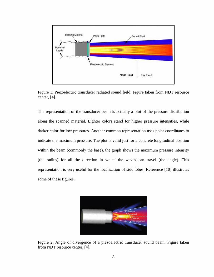
(Figure 1) [9].

(12)

8

Figure 1. Piezoelectric transducer radiated sound field. Figure taken from NDT resource center, [4].

The representation of the transducer beam is actually a plot of the pressure distribution

along the scanned material. Lighter colors stand for higher pressure intensities, while

darker color for low pressures. Another common representation uses polar coordinates to

indicate the maximum pressure. The plot is valid just for a concrete longitudinal position

within the beam (commonly the base), the graph shows the maximum pressure intensity

(the radius) for all the direction in which the waves can travel (the angle). This

representation is very useful for the localization of side lobes. Reference [10] illustrates

some of these figures.

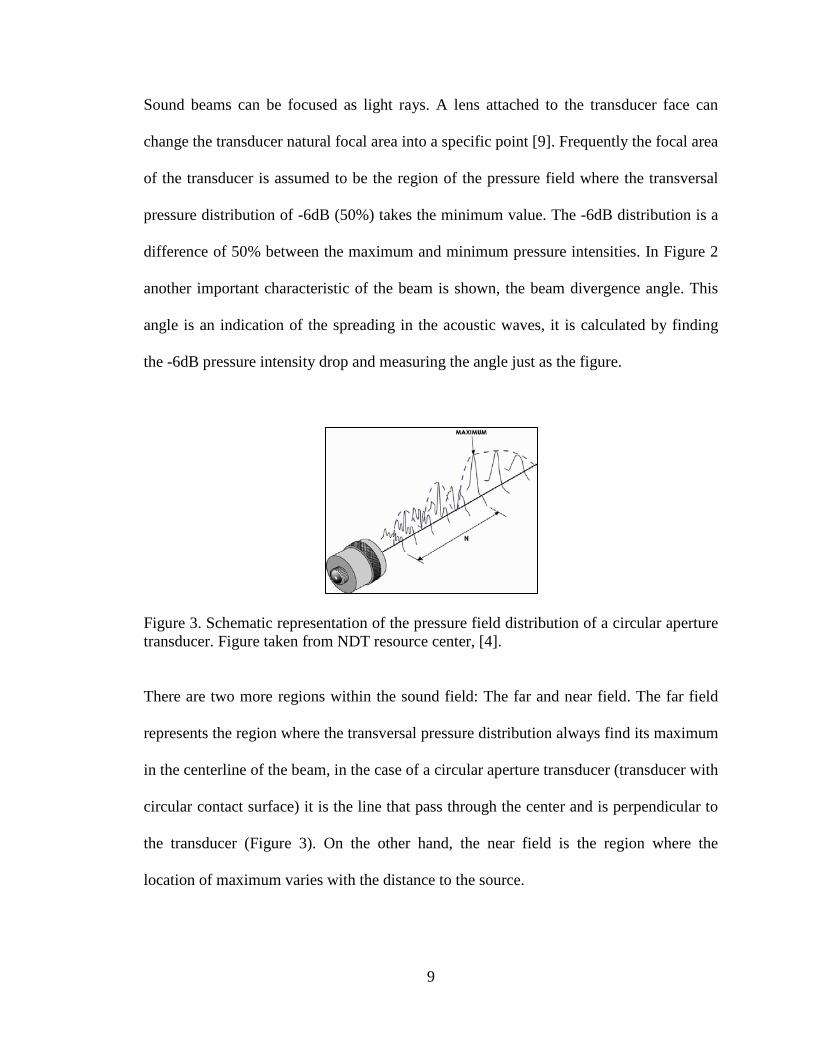
Figure 2. Angle of divergence of a piezoelectric transducer sound beam. Figure taken from NDT resource center, [4].

9

Sound beams can be focused as light rays. A lens attached to the transducer face can

change the transducer natural focal area into a specific point [9]. Frequently the focal area

of the transducer is assumed to be the region of the pressure field where the transversal

pressure distribution of -6dB (50%) takes the minimum value. The -6dB distribution is a

difference of 50% between the maximum and minimum pressure intensities. In Figure 2

another important characteristic of the beam is shown, the beam divergence angle. This

angle is an indication of the spreading in the acoustic waves, it is calculated by finding

the -6dB pressure intensity drop and measuring the angle just as the figure.

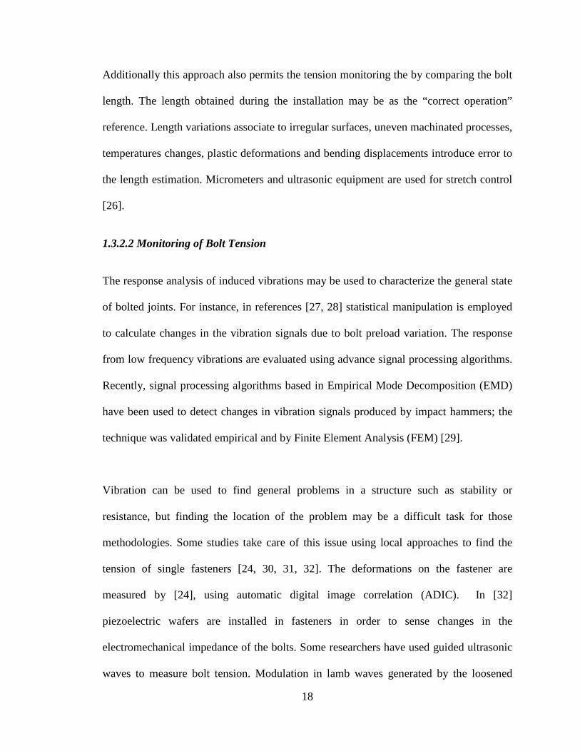
Figure 3. Schematic representation of the pressure field distribution of a circular aperture transducer. Figure taken from NDT resource center, [4].

There are two more regions within the sound field: The far and near field. The far field

represents the region where the transversal pressure distribution always find its maximum

in the centerline of the beam, in the case of a circular aperture transducer (transducer with

circular contact surface) it is the line that pass through the center and is perpendicular to

the transducer (Figure 3). On the other hand, the near field is the region where the

location of maximum varies with the distance to the source.

10

The end of the near field is the point of maximum transverse relative intensity within the

focal area, also known as the natural focus. The Fresnel approximation of spatial

diffraction can be used to calculate the exact pressure distribution of a specific beam.

Detailed explanation of the methodology can be found in reference [9]. A common

approximation of the length of the near field (N) for P-waves generated by circular

aperture PZT is the following [10]:

𝑁 = 𝐷2𝑓4𝐶𝐿

Where N is the length of the near field, D is the diameter of the circular aperture, f is the

wave frequency and CL is the longitudinal wave velocity.

1.2 Real Area of Contact

The surface of a solid material can be described as a series of micro scaled peaks and

valleys with a specific pattern which determines the rugosity of the surfaces. Usually the

heights of those peaks have a random behavior represented by a normal Gaussian

distribution [11]. The existence of peaks in rough surfaces implies a very interesting

phenomenon: solid materials touch each other only in the discrete areas where the peaks

tips collide. The summation of the microareas of contact is known as the “real area of

contact” (RAC) [12].

(13)

11

Although the RAC is a parameter related directly to the friction force, it is not commonly

employed in practice. This is due to simple fact that it is impractical to measure the RAC.

The Amontons-Coulomb law, a.k.a “Dry Friction Law”, uses a simple methodology to

calculate the friction force (F). It states that F is directly proportional to the force normal

to surfaces in contact (N) and that the proportionally coefficient is the “coefficient of

friction” (μ) [13]:

F = µN

One can imply from the dry friction law that the RAC is not involved in the friction force

creation, but that is not the case. Indeed, it is in the RAC where all interactions between

the solids in contact take place [12]. The formation of friction force in the RAC is

explained by the interaction among molecules and the mechanical deformation of the

peaks. The molecules build up adhesive forces due to electromechanical relations:

Vander Waal forces, ionic, covalent and metallic links. These connections between

molecules generate opposition to the relative movement among objects.

In addition to the molecular forces, the friction force is completed by the mechanical

resistance of the peak tips. The peaks must suffer plastic and/or elastic deformations

before any relative movement can be produced [12].

Several researchers have shown that the RAC is in fact proportional to the normal force

when either elastic or plastic deformations are present [11, 12, 13]. The presence of only

elastic deformations of the peaks implies the existence of a constant mean micro contact

(14)

12

area (a). Further increments of RAC during this condition are produced by multiplication

of peaks in contact (n) [11]:

RAC = ∑ an1 = n × a

1.3 Bolted Joints

The threaded fasteners are one of the most versatile methods for assembly of structural

components. In bridges, for example, large bolts are used to fix base columns and small

bolts are used to support access ladders. Naturally not all bolts are critical for the

structure operation. Fasteners loaded with small forces and present in large quantities do

not receive the same treatment as the critical bolts. Typical maintenance operations such

tension measurements, internal stress checking or monitoring of crack development are

not practical due to cost and time constrains. Although failure of a single non-critical

fastener is not a significant thread to the structure’s stability, massive malfunction may

cause structural problem such as insufficient stiffness or excessive vibrations.

In the following sections some generalities of bolted joints are presented, definition of

relevant parameters such as bolt preload and pitch are explained. The last section is a

recompilation of some methodologies used for bolt tension measurement and control.

1.3.1 Standards and Definitions of Bolted Joints

1.3.1.1 The Joint Clamping Force

The clamping force (CF) is the force that maintains together the elements of the joint. If

the CF is too low (loosened bolts), separation and bolt fatigue may occur [14]. On the

(15)

13

other hand, excessive CF may produce damages in the members such as excessive

distortion or breakage. More complex phenomena like stress corrosion and hydrogen

embrittlement may be caused by excessive CF [14].

1.3.1.2 Loosening Process in Bolts

The loosening process is explained as a progressive “slip” at the thread-plate and head-

plate interfaces [15, 16, 17, 18]. The “slip” is mainly caused by direct and indirect shear

loads applied to the joint [19, 20]. The bolt tension also tends to loosen the bolt due to the

generation of a loosening moment produced by the helical shape of the thread [19].

Another factor that contributes significantly to the loosening process is the elastic

deformation suffered by the clamped members. It causes direct slip in the bolt head and

build up the loosening moment in the bolt threads [19].

1.3.1.3 Standard Bolts

The standards of the threaded fasteners employ specific terminology for the parameters

that define the general geometry of bolts. In Figure 4 the most important parameters are

illustrated. The pitch is separation between two contiguous threads. The nominal

diameter is the largest diameter of the screw thread. The bolt length is measure from the

head base. The thread length is the distance from the bolt end to the beginning of the

screw thread [21].

14

Figure 4. Geometrical characteristics of bolts.

The bolts ultimate and yield strength are standardized by 3 different parties: SAE, ASTM

and International Metric. Every one of them catalogues the bolts according to the

mechanical strength and the size range. Table 1 presents some examples of the

categorization.

Table 1. Equivalent bolt categorization for standards SAE, ASMT and metric. Designation Size Range Minimum Yield strength

SAE Grade 8 ¼ - 4 in 130 Kpsi

ASTM A354 grade BD ¼ - 4 in 130 Kpsi

Metric 10.9 M5-M36 (mm) 830MPa

15

1.3.1.4 The Bolt Tension

The CF is generated by the superposition of the individual tension of the bolts present in

the joint. The bolt tension, a.k.a bolt preload, is the actual force that is stretching the bolt

body. The preload is related to the relative stiffness of the bolt and clamped members. In

order to calculate the required bolt tension for generating a specific CF, the interaction

between the bolt and the members should be modeled as three springs in series. In

reference [21], a complete procedure for finding the CF by the application of a specific

bolt tension is presented.

1.3.2 Measuring and Controlling the Bolt Tension

There are two different stages in the operation of bolted joints that require tension

control: Assembly and regular operation. Geometric characteristics like the stiffness or

bolt position usually do not change during the assembly or the regular operation. This is

the reason why the accurate tension control is necessary to ensure a correct CF [22]. In

the assembly process, the tension is controlled to guarantee a correct preload and

therefore the correct CF. On the other hand in the regular operation, the tension is

monitored to ensure a safe CF level during the joint life.

1.3.2.1 Control of Preload in Bolted Joints

There are 4 basic methodologies used to control preload: Torque Control, Turn-Of-Nut

method, Direct Preload Control and Stretch Control.

16

1.3.2.1.1 Torque Control

The torque control is the most used method for controlling bolt tension. Torque wrenches

of manual, pneumatic and hydraulic implementation are common in the market. These

allow the user to apply a large range of torque values and accuracies [23]. The inherent

dependency of this method on uncertain variables such as friction factor, torsion bending

and threads plastic deformation, reduces the accuracy of the applied tension to 25%-30%

[23, 24].

A common methodology for calculating the torque required for achieving a specific

tension in the bolt is presented by [21]. The formulation uses a modified friction factor

(K) to relate the torque to a specific tension:

𝑇 = 𝐾𝐴𝑡0.85𝑆𝑦𝑑

Where K is the friction factor, At is the tensile stress area, Sy is the bolt yield strength, d is

the bolt nominal diameter and T is the torque applied. A usual approximation for K is 0.2.

1.3.2.1.2 Turn-of- Nut Control

This method consists of two stages. In the first phase the bolt is tightened with a

conventional torque wrench until it reaches approximately 75% of the material ultimate

strength [25]. The second stage involved a turn of 180° after the first tightening. Every

turn of the bolt increases the bolt length (and therefore the tension) by an amount close to

the bolt pitch. The final turn almost assure a tension levels that surpass the bolt yield

point [25].

(16)

17

This 2-step methodology has a tension accuracy of 5%, but can only be used in fasteners

with ductile materials and long and well-defined elastic deformation regions [25].

1.3.2.1.3 Direct Preload Control

This category refers to methodologies that use direct estimators of the tension such as

strains, stress or deformations. Strain gages can measure very precisely strain in the bolts

or in the clamped elements. Knowledge of the bolt strain leads to tension estimation with

accuracy of around 1% [26]. Washers with special designs suffer plastic deformation in

the tightening process and show an indicator when a specific tension is reached. These

crush washers have accuracy of about 4%-10% [26]. In addition to strain and

deformation, rupture is also used to estimate bolt tension. Tension control bolts have

special heads that break when a specific preload is achieved. The main issue with these

methodologies is the high cost of the individual fasteners; calibration may also be a

problem.

1.3.2.1.4 Stretch Control

The bolt tension can be calculated using the Hook’s law of elasticity. The law states that

the stress produced in the bolt body by the preload is proportional to the bolt elongation.

The stretch control uses measurements of the bolt length changes to estimate stress in the

bolt and therefore preload. This approach does not involve any interactions of the bolt

with the plate, which erase any uncertainties due to friction. Furthermore the literature

availability of very precise elastic properties provides to methodology the accuracy of the

instrument used to measure the bolt elongation [26].

18

Additionally this approach also permits the tension monitoring the by comparing the bolt

length. The length obtained during the installation may be as the “correct operation”

reference. Length variations associate to irregular surfaces, uneven machinated processes,

temperatures changes, plastic deformations and bending displacements introduce error to

the length estimation. Micrometers and ultrasonic equipment are used for stretch control

[26].

1.3.2.2 Monitoring of Bolt Tension

The response analysis of induced vibrations may be used to characterize the general state

of bolted joints. For instance, in references [27, 28] statistical manipulation is employed

to calculate changes in the vibration signals due to bolt preload variation. The response

from low frequency vibrations are evaluated using advance signal processing algorithms.

Recently, signal processing algorithms based in Empirical Mode Decomposition (EMD)

have been used to detect changes in vibration signals produced by impact hammers; the

technique was validated empirical and by Finite Element Analysis (FEM) [29].

Vibration can be used to find general problems in a structure such as stability or

resistance, but finding the location of the problem may be a difficult task for those

methodologies. Some studies take care of this issue using local approaches to find the

tension of single fasteners [24, 30, 31, 32]. The deformations on the fastener are

measured by [24], using automatic digital image correlation (ADIC). In [32]

piezoelectric wafers are installed in fasteners in order to sense changes in the

electromechanical impedance of the bolts. Some researchers have used guided ultrasonic

waves to measure bolt tension. Modulation in lamb waves generated by the loosened

19

bolts is used by [30] to calculate a joint damage index. Transformation between the wave

modes due to stress is exploited by [31] with the purpose of calculating stress levels,

tension and CF in the threaded joints.

20

CHAPTER 2: STRUCTURAL HEALTH MONITORING

2.1 Introduction to Structural Health Monitoring

A crucial step in the mechanical design components is the prediction of their operative

life. Uncertain loads, ambient conditions, material properties or even misuse are some of

the cases that a designer has to overcome in order to predict the life of a specific

component. Usually, security factors and redundant designs assure structural integrity

even in the worst case scenarios. These contingencies generate problems such as

increased cost, less efficient designs or over dimensioned structures. Furthermore designs

that support human lives, like airplanes or civil structures, have additional constrains.

The necessity to predict the operative life of components, urged the creation of methods

that permit the monitoring of the “health” of structures. The methods that are able to do it

without damaging the monitored parts are called non-destructive evaluation (NDE). The

principal problem associated with NDE is the necessity of off-line evaluation of

components. NDE techniques need very controlled conditions during evaluation

processes which normally involve disassembly or service leaving of the monitored

component. This kind of monitoring is very common in maintenance programs of any

kind of machinery or structure [33].

21

Structural health monitoring (SHM) overcomes this concrete problem: the evaluation of

health is done while the component or structure is in operation. There are two types of

SHM according to its monitoring approach. The first kind is called passive SHM, it

compares the behavior of the structure while is aging with the original or “brand new”

behavior [33]. The second uses inspection of the components to find actual problems in

the structures, this is called active SHM [33].

2.1.1 Passive Structural Health Monitoring

A very clever way to establish the general health of a structure is finding changes in

specific properties that can be related to explicit problems. For instance, the elevated

temperature in a motor output shaft can be caused due to friction problems. Taking a

thermography of a shaft with bearing problems and comparing it with one with optimal

conditions may show an increased temperature profile. Then the general state of motor

bearings can be monitored by a specific program of thermography [34]. Similar results

can be achieved by measuring vibration or monitoring stress levels in critical locations.

Even some parameters of machines such as current, velocity or torque can indicate

misaligns or bearing failure [34].

Static structures can also be monitored. For instance, [35] presented a statistical method

to estimate growing rate and size of cracks in metallic structures by using piezoelectric

transducers (PZT). The method consists of the calculation of the change in signal

parameters such as peak to peak variation, amplitude variance, root mean square,

kurtosis, crest factor and k-factor.

22

2.1.2 Active Structural Health Monitoring

Non-destructive evaluation (NDE) generally is very meticulous and requires that the part

to be inspected stop working. The best way to avoid this problem is integrating the NDE

into the structure itself. It permits the evaluation and analysis of the structural health

every time it is needed and it does not interrupt the normal operation of the part. This

approach is called active structural health monitoring.

The ultrasonic technologies have a bright future in the active SHM due to the capacity of

scanning relative large areas with low power consumption, good accuracy and low cost

[33]. The piezoelectric wafer transducers (PWT) are small in size and hence they can be

easily embedded in the actual structures.

The accuracy of embedded piezoelectric transducers is discussed by [36]. A laser beam is

employed to produce Lamb waves in the scanned part while embedded PZT receive the

signals. An image generation algorithm is tested for finding flaws three different

applications: An elbow pipe joint, a carbon fiber reinforced plastic plate and a stringer-

skin joint. In the last application Lee et al. try to detect a stringer-skin disbond [36].

Different wave behaviors are captured with different PZT position. It is concluded that

positioning the transducer in the stringer and generating the waves in the skin permits

establishing the dimension of the disbond and some additional details such as the “kissed

part”. Additional applications of active SHM are presented in references [37-46].

23

2.2 Structural Health Monitoring Methodologies using Piezoelectric Transducers

Some methodologies for PZT based SHM are presented in this section. The general

principles, strengths and weaknesses of every technique are reviewed and applications are

discussed. More details and explanation of the methods following presented can be found

in the references.

2.2.1.Electromechanical Impedance

The electromechanical impedance method use PZT to sense the mechanical impedance of

the tested structure. Changes in the mechanical impedance are attributed to the mass or

stiffness changes, therefore it is a reliable parameter for the inspection of the general

health of a structure [37, 38]. This approach is also used in vibration methods such as the

frequency response functions [37]. A PZT attached to a vibrating structure reacts by

changing its electrical impedance [39]; this phenomenon is known as the

electromechanical effect. The real portion of the device impedance is normally used as

the leading parameter in SHM [37], authors as Liang et al. (1994) and Bhalla and Soh

(2003) developed models that demonstrate the reason for such behavior [40, 41].

The electromechanical impedance has some advantages over other SHM methodologies.

Compared to regular vibration methods, this method use much higher frequencies (in the

KHz order), which make it much more sensitive. The electromechanical impedance can

almost be as sensitive as regular ultrasonic NDT approaches but it requires less

complicated equipment and the analysis does not require an expert for interpretation [37].

Compared with other vibration approaches, the electromechanical impedance allows

24

sensors and actuators with self-diagnostic capabilities and low vibration interference,

which permit very accuracy results.

Modeling the relation of electrical impedance of the PZT with the mechanical impedance

is required for fully understanding the structural problems. Finding an accurate

relationship of the electrical response to mechanical excitation is the principal drawback

of this methodology [39]. The common applications of the electromechanical method are

small machinery parts with natural frequencies in the KHz order, a good example of this

are aircraft turbo-engine blades [39].

2.2.2 Ultrasonic Methodologies: Piezoelectric Transducers

Analyzing the response of a structure to specific ultrasonic impulses can lead to

estimation of structural problems such as inadequate stiffness, mass loss or even crack

growing. Following some methodologies that use ultrasonic waves produced by

piezoelectric transducers in order to detect such defects is presented.

2.2.2.1 Pitch and Catch

The pitch and catch technique refers to the employment of two different transducers to

send and receive guided waves. The waves are sent from the transmitting transducer (T)

and acquired by the receiving transducer (R) with information about the material present

between them. The waves used in the pitch and catch technique are generally guided

waves that can be strongly influenced by small variations in the stiffness or thickness of

the material [42] . The pristine condition of the part to be evaluated is taken as baseline

for variation of the waves. Modifications in amplitude, dispersion, phase or time of flight

25

are indicatives of changes in the structure of the monitored part. Lamb waves of different

modes are used commonly with this technique.

The principal strength of the pitch and catch method is its high sensitivity to local

structural problems such as cracks, corrosion or disbands [42]. This technique can be

used for manual inspection in schedule maintenance activities or as automatic monitoring

system. The technique is especially useful in composite structures [42].

Limited space between two transducers is a drawback of this methodology. The waves

only provide information from the material in-between the transducers. Filtering the

acoustic signal may be a necessity for very detailed analysis. For instance, [43] develops

a filtering algorithm for diminishing ringing effects which are common in the imaging

generation of concrete structures using pitch and catch techniques.

The pitch and catch technique is commonly used for debonding detection. In reference

[43], a pitch and catch application with SAW is used to find structural problems in carbon

fiber-reinforced polymers (CFRP) attached to concrete specimens. The research shows

the capability of the technology to monitor the structural health of the specimens and

explain the effectiveness of the methodology. In reference [30], Lamb wave modulation

is used to estimate stiffness problems in a bolted joint. The authors calculate a damage

index of the joint based in the wave modulation. In reference [42], additional realized

applications for this methodology can be founded.

26

2.2.2.2 Pulse-Echo

The principle of operation the pulse-echo method is based in the reflection of acoustic

waves. The waves generated in the material are partially reflected by holes, corrosion,

dibonding and other defects. The reflected waves carry information that is received by the

transducer. The time that it takes for the waves to hit and return to the transducer is

called time of flight (TOF). The TOF provides the position of the reflective boundary

[33]. The amplitude and frequency of the reflected waves may be used to estimate the

size and shape of the defects. Pressure waves are normally employed for through-the-

thickness pulse-echo scanning and guided waves such as Lamb or SAW are used for

longitudinal monitoring [33]. This technique is used in the experiments presented in

Chapters 3 and 4.

The simple configuration of the methodology is very advantageous for manual and

automated structural monitoring [42]. Regularly only one PZT is used as receiver and

transmitter which reduce costs and set up time. This technique is generally employed for

imaging generation due to its inherent capacity for defect localization. By mapping the

reflection location of all the reflective points, an image with the size and position of all

the features in the scanned area can be created. Imaging generation is explained in the

final section of this chapter.

The principal limitation associate with this method is the difficulty of differentiating

boundaries that are close to each other. Proximate defects tend to create reflections that

superpose while traveling through the scanned material. Separating the individual effect

27

of each one is critical for a good signal analysis [42]. In some cases this procedure cannot

be done correctly, which lead to errors in the estimation of size and position of the flaws.

Also, the waves employed in the pulse-echo approach generally should be low dispersive

in nature such as bulk waves or SAW.

Application of the pulse-echo approach can be found from medical imaging to concrete

pipes monitoring. In reference [44] ultrasound based techniques for concrete pipe

inspection are presented. The pulse-echo methodology is presented as a viable approach

for cracks, fractures and holes detection. Air-coupled pulse-echo is shown in [45], impact

hammers generate ultrasound vibration in a concrete plate with artificial generated

defects. The waves are then transmitted to the air where a specially insulated microphone

receives the signal. The microphone is moved along the plate to create an image based on

the frequency changes of the received waves.

2.2.3 Ultrasonic Methodologies: Transducer Arrays

Instead of creating an acoustic beam with a single PZT, a defined number of transducers

are placed in a specific configuration in order to generate a controlled beam [46]. The

increased number of waves that are created by the array allows the creation of images at

every test location, which is an obvious decrease in the manual scanning times. Arrays

may also be used as flaw radars in metal structures, they can be electronically controlled

to scan large areas without the necessity of moving parts [47].

The generation of images is based in the reflected waves created by changes of acoustic

impedance inside the material, just as the regular pulse-echo approach. Additionally, the

28

arrays are able to focus and steer the generated and received signals by applying delays

and gains in the elements. This enables to suppress the generation and reception of waves

that propagate in undesired directions [47]. In the following sections two array

geometries are presented: Linear arrays and 2-D arrays. The principal characteristic of the

arrays along with beam formation capabilities and applications is explained.

2.2.3.1 Linear Arrays

A linear array is defined by 3 important parameters: Pitch, number of elements and

element width (Figure 5) [47]. Normally the element width is much smaller than the

element length, so it is commonly modeled as semi-infinite plate with undefined length.

This characteristic makes the linear arrays insensitive to the longitudinal direction of the

element, therefore only plane images can be generated through linear arrays [46].

Figure 5. Sketch of linear array geometry

A great advantage of the transducer arrays over the single transducer approach is the

capacity to create a common acoustic beam. While a single transducer cannot change its

29

characteristic beam, the waves generated by several transducers can be combined to

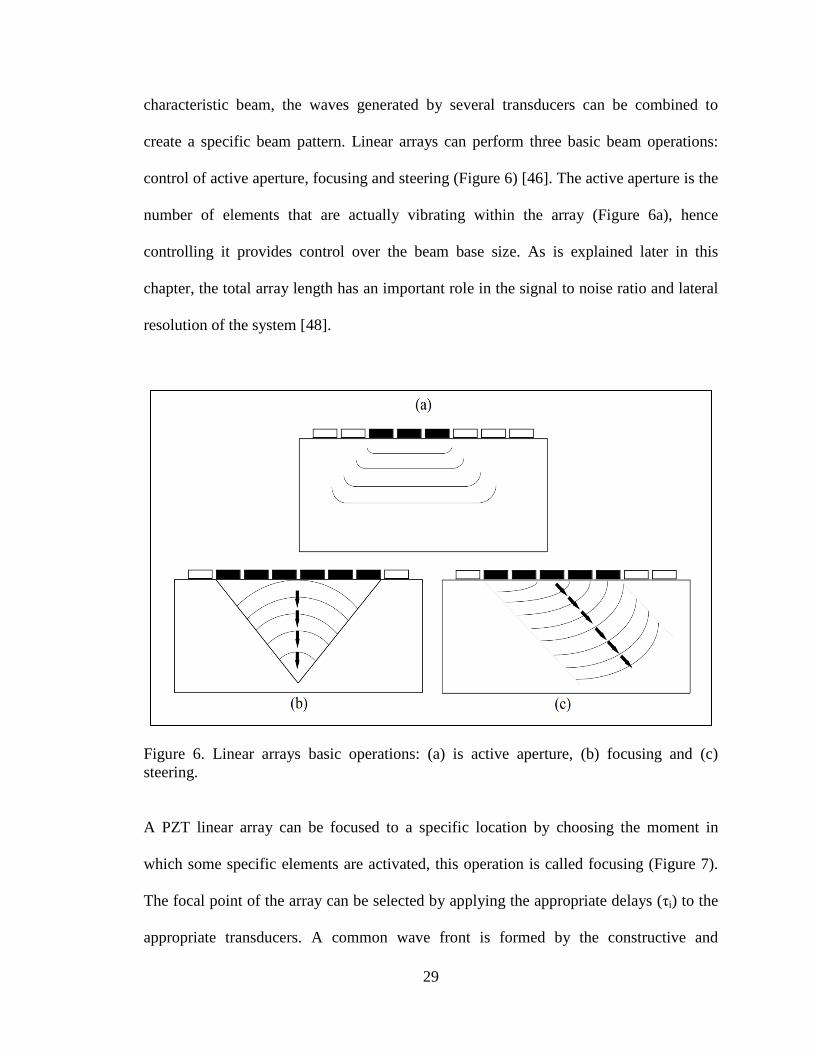
create a specific beam pattern. Linear arrays can perform three basic beam operations:

control of active aperture, focusing and steering (Figure 6) [46]. The active aperture is the

number of elements that are actually vibrating within the array (Figure 6a), hence

controlling it provides control over the beam base size. As is explained later in this

chapter, the total array length has an important role in the signal to noise ratio and lateral

resolution of the system [48].

Figure 6. Linear arrays basic operations: (a) is active aperture, (b) focusing and (c) steering.

A PZT linear array can be focused to a specific location by choosing the moment in

which some specific elements are activated, this operation is called focusing (Figure 7).

The focal point of the array can be selected by applying the appropriate delays (τi) to the

appropriate transducers. A common wave front is formed by the constructive and

30

destructive interferences of the waves created by the single elements. The wave front is a

new beam focused into a desired location [49]. The following formulation shows the

calculation procedure of the delay times [50]:

𝜏𝑖 =𝑥𝑖−𝑥𝑓

2+𝑦𝑖−𝑦𝑓2

𝐶− 𝑅𝑓

𝐶

Where τi is the delay time of the ith element, xi and yi are the coordinates of the ith

element, xf and yf are the coordinates of the desired focal point, C is the speed of sound of

the scanned material and Rf is the distance of the focal point to the array center.

Figure 7. Schematic of linear array focusing.

Beam steering is also achieved by delaying the activation of some elements. The overall

beam is rotated a desired angle (Figure 8). This increase the scanning capacity of the

array, but it can also create undesired beams known as beam side lobes. The lobes are

created by the interaction of out of phase waves generated by the array elements. A

common strategy to avoid its creation is reducing the array pitch. In [49] it is explained

that for a pitch smaller that λ/2 the side lobes disappear.

(17)

31

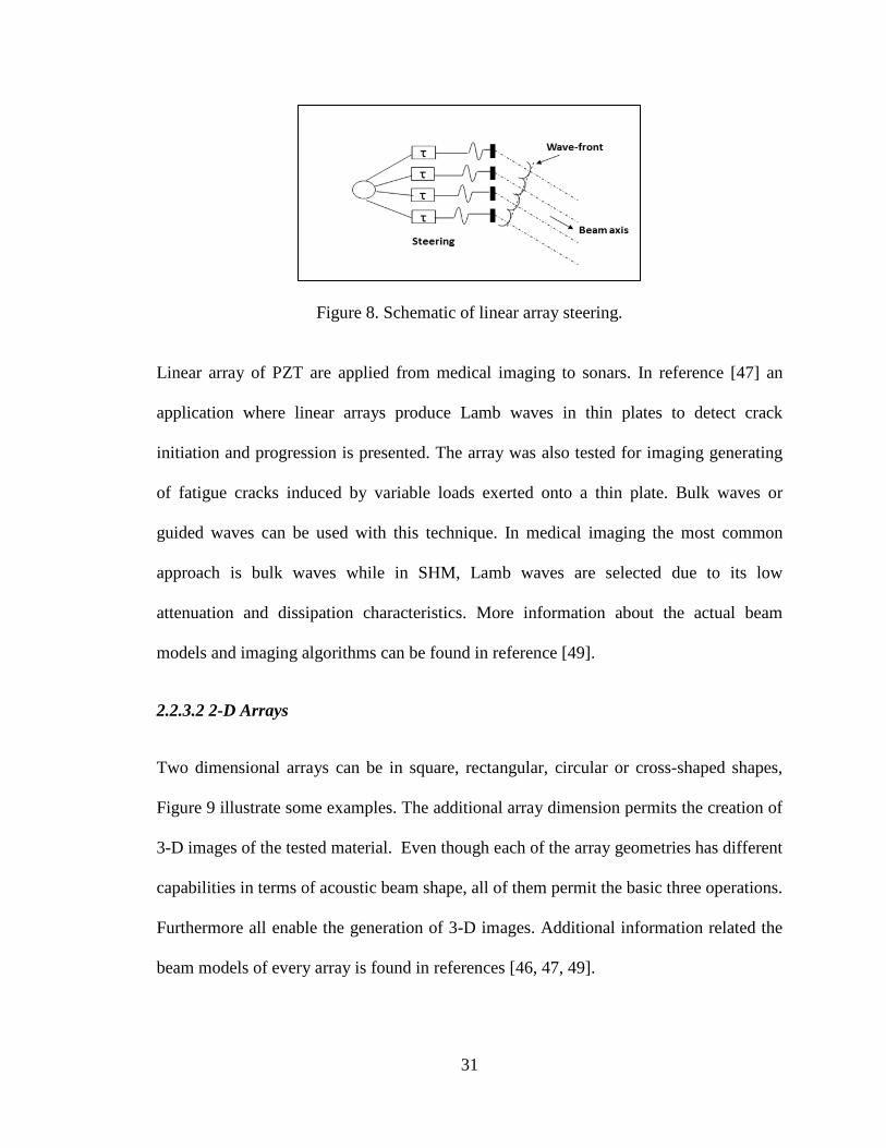
Figure 8. Schematic of linear array steering.

Linear array of PZT are applied from medical imaging to sonars. In reference [47] an

application where linear arrays produce Lamb waves in thin plates to detect crack

initiation and progression is presented. The array was also tested for imaging generating

of fatigue cracks induced by variable loads exerted onto a thin plate. Bulk waves or

guided waves can be used with this technique. In medical imaging the most common

approach is bulk waves while in SHM, Lamb waves are selected due to its low

attenuation and dissipation characteristics. More information about the actual beam

models and imaging algorithms can be found in reference [49].

2.2.3.2 2-D Arrays

Two dimensional arrays can be in square, rectangular, circular or cross-shaped shapes,

Figure 9 illustrate some examples. The additional array dimension permits the creation of

3-D images of the tested material. Even though each of the array geometries has different

capabilities in terms of acoustic beam shape, all of them permit the basic three operations.

Furthermore all enable the generation of 3-D images. Additional information related the

beam models of every array is found in references [46, 47, 49].

32

Figure 9. Schematics of 2-D arrays geometries: (a) Cross configuration, (b) Square configuration, (c) Rectangular configuration (a.k.a 1.5-D [46]) and (d) Circular configuration

Application of 2-D arrays can be found in medical imaging, sonars and SHM. In

reference [47] several experiments for damage detection using different arrays are

presented. The author also presents active aperture algorithms for the design of damage

detection radars in thin plates. The main issue with 2-D arrays is the number of

independent transmits-receive channels required for operation. The current technology

allows up to 256 [46]. The number of channels represents the number of elements that

can be active in the scanning process (active aperture), this obviously constrains the 2-D

arrays hence they great quantity of element (per unit size) required.

2.2.4 Ultrasonic Image Generation

Critical structural problems can be detected with ultrasonic imaging. Corrosion, cracks or

even missing bolts can be found with ultrasonic images. In this section two

33

methodologies used for image formation based in PZT arrays are presented. General

principles of beam generation and image reconstruction are explained; the quality factors

of an image system are defined and described.

An ultrasonic image, as the one illustrated in Figure 10, is a geometrical representation of

the waves generated in a scanned object. The nature of the wave (Lamb, pressure, shear,

etc.) does not change the way the representation is made: high amplitude waves are

presented in a specific color and low amplitude in another. In the case of the Figure 10,

white is high intensity and black low amplitude. In most imaging system the

representation is based in the reflected waves created by the difference in acoustic

impedance of the scanned media; the higher the difference, the higher intensity of the

reflected wave.

Figure 10. Example of an ultrasonic image.

The wave intensity is received by signal collector as a voltage value, so a strong acoustic

impedance change is received by the collector as a bigger voltage peak. In summary, an

acoustic image is a geometrical array where different voltage values, collected by PZT,

34

are displayed in congruent color scale with the goal of showing the differences in

acoustic impedance present in the scanned material.

2.2.4.1 Phased Array Imaging

This technique uses simultaneously all the array elements as transmitters and receivers.

The goal is to produce a focused beam in a desired direction in order to increase the

signal to noise ratio and therefore obtain higher resolution images [50, 51]. The main

drawback of this approach is the high complexity in electronics, especially in arrays with

large number of elements. It is necessary to have a large number of transmit and receive

channels active at the same time during the image formation [50]. The successful

application of this methodology in the medical field has leaded the researches to explore

applications in non-destructive testing. Some representative applications are presented in

references [62-68].

By applying the appropriate delays to the array elements, the complete array beam is

focused into a desired direction. Progressively the array focus direction is changed in

order to scan a different line of the scanned area. This is 2-D polar scanning sequence,

with the steering angle representing the angular coordinate.

The reflection signals are delayed, focused and added just as the generated signal were.

This is not an electronic procedure like the case of generation which consist of delaying

the input voltage, but an off line correction of the data that are added together. The same

delay time (τi) used for focusing is now used to find the data point that correspond to

35

every specific image point (pixel). The reconstructed signals correspondents to a specific

steering angle are calculated using the following expression [50]:

𝑟𝜃(𝑡) = ∑ ∑ 𝑤𝑗𝑤𝑖𝑠 𝑡 −𝑅𝑓𝐶− 𝜏𝑗𝑁

𝑗=1𝑁𝑖=1

Where wj is a weighting parameter, mostly used for attenuation adjustments, sj(t) is the

actual signal received by the jth transducer, Rf is the distance from the reconstructed point

to the array center, C is the sound speed velocity of the scanned material, τj is the time

delay correspondent to the jth element, N is the total number of transducers and finally

rθ(t) is reconstructed signal correspondent to the θ angle.

The final step in the image formation is coordinate conversion and interpolation. The

polar signal arrangement (rθ) is converted to Cartesian coordinates:

𝑟 = 𝑥2 + 𝑦2 & 𝜃 = arcsin 𝑦𝑥

Where x and y are the Cartesian coordinates of the desired pixel. In order to increase the

number of data point which decrease the pixel size and therefore improve the image

resolution, an interpolation is applied to the converted image [50].

2.2.4.2 Synthetic Phased Array Imaging

The synthetic phased array reduces the complexity of the phased array by using only 1

element in transmitter-receiver mode. Two approaches can be used with this method:

conventional synthetic aperture or synthetic phased array. In the conventional synthetic

aperture, 1 transducer is mechanically manipulated in order to create the desired array.

The transducer is transmitter and receiver in different positions. The synthetic phased

array use a real array of transducer but in a particular time only one transducer acts as

(18)

(19)

36

transmitter and receiver. The others elements act as receivers only, this characteristic

permit the increment of the image quality while significantly reducing the system

complexity [50].

Contrary to the phased array approach, in the synthetic array methodology, the acoustic

beam is not focused on a single point or direction. The beam is produced by a single

element and therefore the beam focus is the natural focus of the transducer. The beam is

expected to generate waves in all the scanned area and the reflection should be detected

for the rest array elements. It is shown in Figure 11 that the transmitter-receiver mode is

alternated within the elements, hence a complete scan only finish when all the elements

have acted as transmitter and receiver [50, 52].

Figure 11. Schematic operation procedure of the synthetic phased array.

The image reconstruction is similar to the phased array approach. The reflection signals

are focused with time delays. In this case the reconstructed signal is a 2-D sector image,

hence all the transducer create an image of the scanned area when a particular transducer

37

is actuated. The images are then added in order to form the final picture. The signal can

be reconstructed following the following formulation [53]:

𝑟(𝑥′, 𝑦′) = ∑ 𝑤𝑗𝑠𝑗 𝑡𝑜 + 2𝐶𝑥′ − 𝑥𝑗

2+ 𝑦′2𝑁

𝑗=1

Where wj is a weighting parameter, mostly used for attenuation adjustments, sj(t) is the

actual signal received by the jth transducer, to is the time needed nullify the effects of the

electronic devices, C is the sound speed velocity of the scanned material, xj is the

transversal position of the jth array element, N is the total number of transducers and

finally rx,y is reconstructed value of the pixel with coordinates (x’,y’).The initial signal s(t)

may be interpolated for increasing the number of pixels in the image and therefore the

image resolution.

Due to the inherent advantages of the synthetic aperture focusing, many studies have

been performed in order to improve its efficiency and its applicability in strongly

attenuative materials. In reference [54, 55, 56] some modified algorithms based in this

methodology have shown improvement in the image quality in very difficult materials

such as concrete and ferritic-austenitic stainless steel.

2.2.4.3 The Performance Criteria of an Imaging System

Four basic parameters define the quality of an acoustic imaging system: Axial resolution,

lateral resolution, contrast resolution and signal to noise ratio (SNR). The axial and

lateral resolution are related to the capacity of the system to separate reflective

boundaries along the longitudinal and transversal beam axis respectively. The axial

resolution is improved by the generation of signals with long bandwidth. This is achieved

(20)

38

with high frequency transducer and short pulses. High frequency waves are affected more

by the attenuation, so lower scanning penetration can be achieved. The axial resolution

can be calculated as follows:

∆𝑙 = 𝐶 𝑡𝑝2

Where l is a longitudinal distance, C the waves propagation velocity and tp is the

temporal pulse length. Δl represents the minimum change in longitudinal distance that

can be measured by the imaging system.

The lateral resolution depends of the beam width, the wider the beam the less resolution.

An image formed close to the beam focus has better resolution than another one formed

in the far or near field [10]. Side lobes also reduce the lateral resolution due to of noise

introduction to the system. The contrast resolution a.k.a dynamic range, is defined as the

smallest change in acoustic impedance that the system is able to measure.

The dynamic range is presented in decibels units (dB). It represents the square

logarithmic ratio between the maximum and minimum signal:

∆𝐼(𝑑𝐵) = 20log 𝑃2𝑃1

The contrast resolution can be improved by reducing the side lobes levels and increasing

the axial and lateral resolution [48]. The signal to noise ratio (SNR) is a method to

measure the amount of information present in the signal relative to the ambient noise.

Low levels of SNR means that the intensity of the reflected waves is comparable to

ambient noise which cause low quality images. Alternatives to increase the SNR are the

increment in the array element size and averaging the received signal.

(22)

(21)

39

CHAPTER 3: INSPECTION OF STEEL PLATES VIA ULTRASONIC

ACOUSTIC WAVES

3.1 Calculation of Surface Acoustic Wave Velocity in Steel 1018.

A very important characteristic of the surface acoustic waves (SAW) is the constant wave

velocity. The imaging reconstruction techniques take advantage of this fact to estimate

the position of reflective boundaries within the scanned material. The application of

accurate wave velocity values is necessary for a precise image reconstruction. Although

there is an explicit formulation to obtain SAW velocity, the natural variation of the

material properties involved in the formulation may potentially cause significant errors.

In order to overcome this problem, the estimation of the SAW velocity in a 1018 steel

plate is carried out in the following experiment. Additionally, the results are compared

with the theoretical velocity founded in the published literature.

3.1.1 Experiment Configuration

The SAW velocity is calculated by measuring the time of flight (TOF) of the waves

reflected by the plate edge. The generation and reception of the SAW is conducted with a

5MHz and ½ in diameter transducer attached to a crystal wedge, a pulse generator

(Olympus 5072PR) and an oscilloscope (Tektronix TDS 2024B). Detailed characteristics

of the device are presented in Appendix A. Figure 12 shows a sketch of the wedge’s

initial position.

40

With the assistance of a manual micrometer, the crystal is positioned 3 inches from the

edge of the plate. The nature of the system requires setting the pulse generator at a

damping of 50Ω and pulse repetition frequency (PRF) of 200Hz and the received signal

amplification to 40dB.

Figure 12. Schematic of the initial position of the wedge.

3.1.2 Procedure

Initially, the wedge with the transducer attached should be positioned at the point

illustrated in Figure 12. After the wedge is correctly positioned, the signal acquired is

recorded by the oscilloscope. No further data recording is required due to the high

accuracy of the oscilloscope. This recorded signal will be used to calculate the SAW

velocity.

3.1.2 Experimental Results

Figure 13 illustrates an example of the acquired signal with the experimental setup

discussed above. There are three clear signal peaks resulted from the interaction with

three different objects. The first peak is caused by the electrical equipment interference.

41

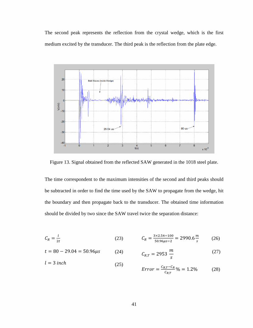
The second peak represents the reflection from the crystal wedge, which is the first

medium excited by the transducer. The third peak is the reflection from the plate edge.

Figure 13. Signal obtained from the reflected SAW generated in the 1018 steel plate.

The time correspondent to the maximum intensities of the second and third peaks should

be subtracted in order to find the time used by the SAW to propagate from the wedge, hit

the boundary and then propagate back to the transducer. The obtained time information

should be divided by two since the SAW travel twice the separation distance:

𝐶𝑅 = 𝑙2𝑡

𝑡 = 80 − 29.04 = 50.96𝜇𝑠

𝑙 = 3 𝑖𝑛𝑐ℎ

𝐶𝑅 = 3×2.54÷10050.96𝜇𝑠÷2

= 2990.6𝑚𝑠

𝐶𝑅,𝑇 = 2953 𝑚𝑠

𝐸𝑟𝑟𝑜𝑟 = 𝐶𝑅,𝑇−𝐶𝑅𝐶𝑅,𝑇

% = 1.2%

(23) (26)

(24) (27)

(25) (28)

42

Where CR represents the surface wave velocity, CR,T is the theoretical surface wave

velocity calculated with the formula illustrated in section 1.1.1.3, t is the time used by the

SAW to go through the plate and go back to the transducer, and l is the distance from the

crystal wedge to the plate edge. The difference of the velocity found with the experiment

and the velocity calculated is very small (1.2%), which means that the acoustic properties

of the 1018 steel plate agree with values found in the literature [57].

3.2 Calculation of SAW Attenuation Coefficients in Steel 1018

A simple experiment is performed in order to calculate the exponential attenuation

coefficient of the propagating SAWs [10, 58]. The attenuation lead to intensity

diminution of the received signal, therefore characterization of flaws based in the signal

intensity can turn to be difficult if the attenuation is not taken into account. The following

experiment shows a method to find the attenuation coefficient of SAW in a 1018 steel

plate.


Diminution in the signal intensity due to increment of the wave time of flight (TOF) is

used to calculate the attenuation coefficient of SAW. The generation SAW is achieved

through a 5MHz transducer attached to a crystal wedge and a pulse generator.

Additionally the transducer-wedge configuration is connected to a translation stage with

the help of specially designed aluminum parts. The SAW are sent in direction of the right

plate edge (Figure 14) in order to catch the wave reflections and save its intensity, the

TOF is increased by changing the wedge separation from the plate edge. An oscilloscope

43

is used to calculate the peak-to-peak value of the received signal; all the specific

information about the equipment is presented in Appendix A.

3.2.2 Procedure

The initial position of the wedge is shown in Figure 14. Using the translation stage the

wedge should be move 0.1in towards the plate edge. Prior to any further movement the

peak-to-peak value of the received signal should be saved. The oscilloscope scale set so

that the peak generated by the electrical devices does not influence the peak-to-peak

calculation. Failure to do so may results in a peak-to-peak intensity correspondent to the

electrical interference. Another important consideration is to maintain the SAW path

towards the plate edge free of acoustic coupling, liquids in contact with plate surfaces

attenuate the incoming SAW due to losses in form of compressional waves [8], so

leaving traces of couplant between the wedge and the plate edge generates attenuation

that is independent from the steel plate.

44

Figure 14. Drawing of initial position of wedge.


The peak-to-peak values versus wedge position are plotted in Figure 15. An exponential

approximation to the curve is also shown. The Figure 15 presents clearly the exponential

behavior of the attenuation factor, it shows an R-squared error of 0.99 for an attenuation

value of α=-0.548 Np/in.

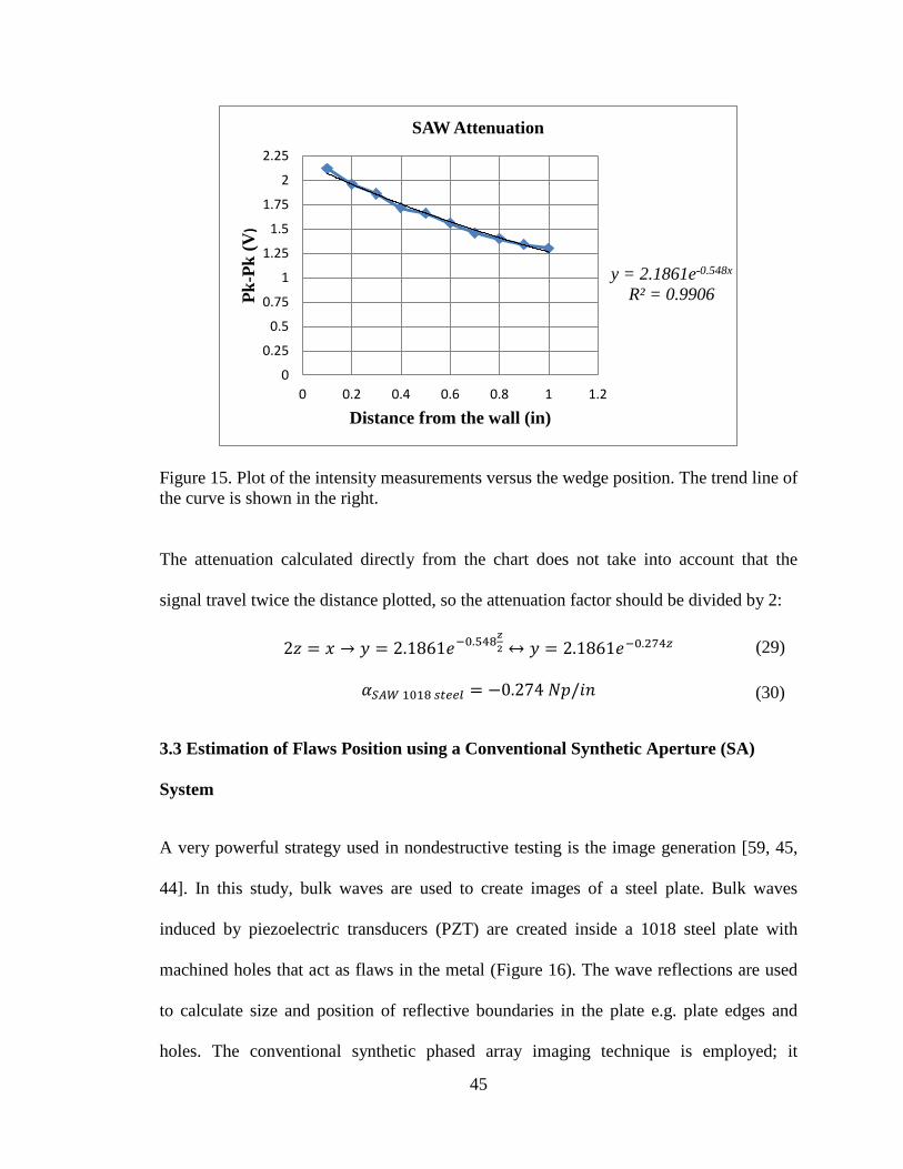
45

Figure 15. Plot of the intensity measurements versus the wedge position. The trend line of the curve is shown in the right.

The attenuation calculated directly from the chart does not take into account that the

signal travel twice the distance plotted, so the attenuation factor should be divided by 2:

2𝑧 = 𝑥 → 𝑦 = 2.1861𝑒−0.548𝑧2 ↔ 𝑦 = 2.1861𝑒−0.274𝑧

𝛼𝑆𝐴𝑊 1018 𝑠𝑡𝑒𝑒𝑙 = −0.274 𝑁𝑝/𝑖𝑛

3.3 Estimation of Flaws Position using a Conventional Synthetic Aperture (SA)

System

A very powerful strategy used in nondestructive testing is the image generation [59, 45,

44]. In this study, bulk waves are used to create images of a steel plate. Bulk waves

induced by piezoelectric transducers (PZT) are created inside a 1018 steel plate with

machined holes that act as flaws in the metal (Figure 16). The wave reflections are used

to calculate size and position of reflective boundaries in the plate e.g. plate edges and

holes. The conventional synthetic phased array imaging technique is employed; it

y = 2.1861e-0.548x R² = 0.9906

0

0.25

0.5

0.75

1

1.25

1.5

1.75

2

2.25

0 0.2 0.4 0.6 0.8 1 1.2

Pk-P

k (V

)

Distance from the wall (in)

SAW Attenuation

(29)

(30)

46

consists of a virtual manipulation of the signals received and generated by a single

transducer actuated from different locations [50]. In this experiment the accuracy of the

technique will be tested with the purpose of finding its suitability in further applications.

In this research an acoustic couplant that follows the standard ASTM F945 is employed.

Figure 16. Photo of the bulk waves experiment configuration.

3.3.1 Experiment Design

The synthetic array design consists of two parameters: the number of elements in the

array and the distance between the members (pitch). The array pitch is inversely related

to the lateral resolution of the imaging system [50], normally it is selected as some

specific fraction of the wavelength (λ), which depends of the bulk wave velocity and the

transducer frequency. The wave frequency (transducer central frequency) is also related

to the axial resolution of the imaging system [48], hence high resolution images required

47

high frequency elements and small pitch arrays. Therefore, in this experiment the highest

frequency transducer available in the facilities (5MHz) is selected. The array pitch (p) is

chosen to be λ/4:

𝑝 = λ4⁄ =

VBulk

4f=

E

ρ 1+υ

1−2υ

4f

𝑝 = 205𝐺𝑝𝑎7870𝑘𝑔/𝑚2

1+0.291−2×0.29

4×5𝑀𝐻𝑧

𝑝 ≈ 0.01𝑖𝑛

Where f is the transducer center frequency, E, ν, ρ are the elasticity modulus, the

Poisson’s ratio and the density of the 1018 steel, respectively. Properties were taken from

[57].

The number of elements in the array (NE) determines the array aperture (length) which is

proportional to the lateral resolution, therefore high number of elements increases the

resolution, at a cost of increasing scanning time, so a balance between image quality and

experiment duration should be determined. In this study, it was decided to create and

array of 55 elements, so the array has an active aperture of 0.55in.

(31)

(32)

(33)

48

Figure 17. Schematic configuration of the bulk wave experiments. A blueprint of the steel block where the position of the holes, the dimensions and the position of the transducer array is presented. The table shows the diameter and position in X and Y coordinates of the holes in the steel block.


A synthetic phased array is created with help of a translator stage (TS). The 1018 steel

plate is secured to the workbench using specially design aluminum clamps. A second set

of aluminum parts connects the transducer to the translator stage and allows the free

movement of both components. In Figure 16 and Figure 17 a real and schematic view of

the configuration is shown. Figure 17 also illustrates the exact position of the machinated

holes and the area that corresponds to the array. Appendix A contains a datasheet of the

devices used in this test.

49

3.3.1.1 Experimental Procedure

1. The steel plate should be positioned in a place that allows to the translation

stage to reach it. The aluminum clamps should lock the steel plate in the

position shown in Figure 16.

2. The wedge-transducer assembly should be secured to the TS with help of the

Aluminum L and aluminum plate. The height of this assembly must permit the

contact between the transducer base and the plate surface. Acoustic couplant

must be applied prior any contact as the acoustic impedance mismatch

between the transducer crystal and the steel may prevent the transmission of

waves.

3. The TS is employed to position the wedge as is shown in Figure 17 (y=6in,

x=1.225in). It is very helpful to use the steel plate edges as reference. The

movement span of the TS is only one inch, so the configuration process

should take into account that the wedge needs to move 0.55in after initially

installed.

4. The oscilloscope and the pulse generator should be turned on. The signal gain

must be set around a value in the range of 20’s or 30’s. The correct

configuration of the oscilloscope allows the edge reflection to be observed.

The highest peak should be at least half of the oscilloscope scale.

50

5. In order to start the recording process, the signal should be set to average, this

helps to increase the signal to noise ratio of the system. After recording the

signal at the initial point, the transducer should be moved 0.01in to the right;

prior to recording the second response, the average function should be reset.

This procedure is repeated until 55 data points are collected.


Longitudinal and transversal images of the steel block are the results of this experiment.

Figure 18 shows full longitudinal images (B-scan) of the steel block, the images are

presented with three dynamic ranges: 10dB, 20dB, 30dB. Higher decibels include

reflections with lower intensity values, which cause images with more details but more

prone to the noise. Images with lower decibels reduce the influence of noise information

but it reduces the perception of signal with lower intensities, as is the case of the deepest

hole set in Figure 18c [50].

51

(a) 30dB (b) 20dB (c)10dB

Figure 18. Longitudinal images of a 1018 steel plate generated by synthetic phased array using bulk waves. Presentation with dynamic range of: (a) 30dB, (b) 20dB and (c) 10dB.

Figure 19 illustrates the full longitudinal images of the plate and also closer view of the

holes for improved details. As expected, the image quality is deteriorated with increased

depth. For instance, the first hole set appears sharp and with some details while the third

hole set register almost no trace of the original geometry. This deterioration is a result of

the low intensity signal received from the deeper holes consequence of the attenuation.

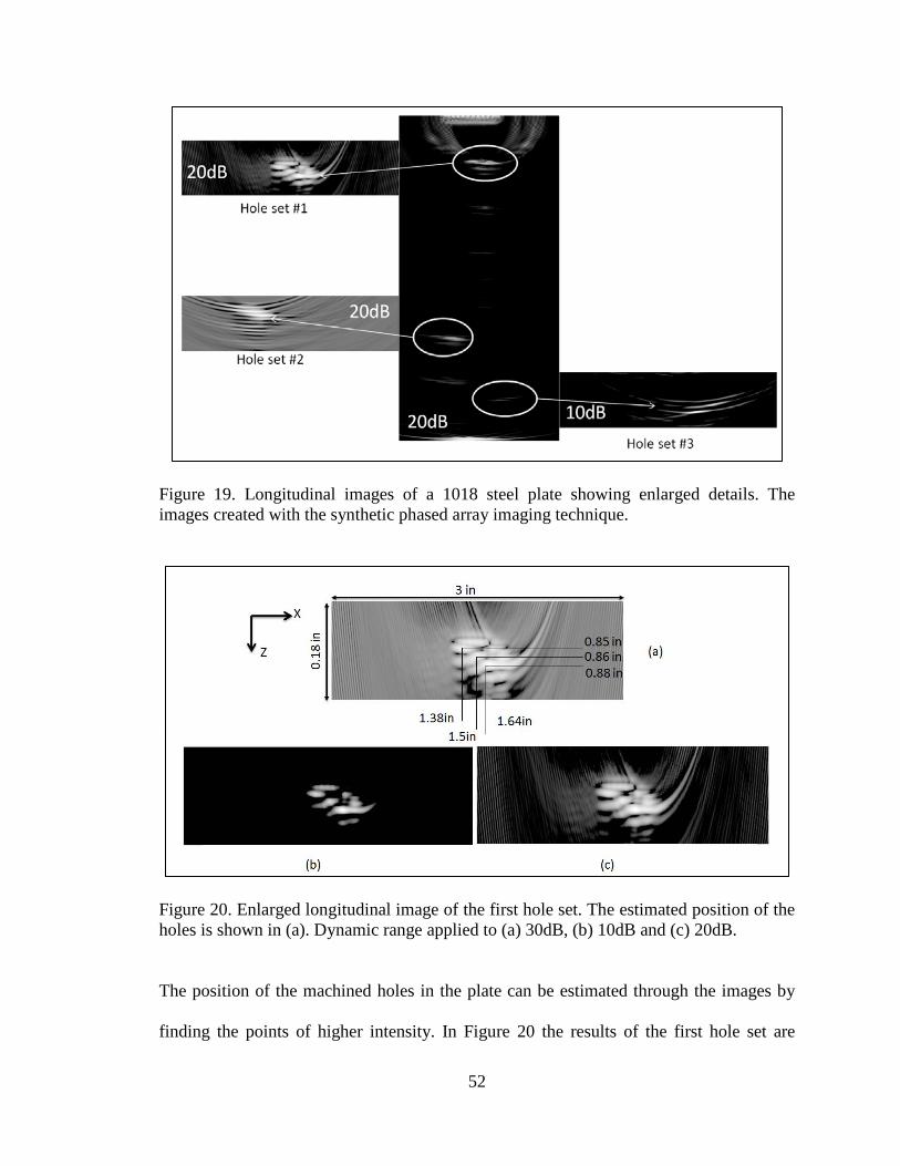
52

Figure 19. Longitudinal images of a 1018 steel plate showing enlarged details. The images created with the synthetic phased array imaging technique.

Figure 20. Enlarged longitudinal image of the first hole set. The estimated position of the holes is shown in (a). Dynamic range applied to (a) 30dB, (b) 10dB and (c) 20dB.

The position of the machined holes in the plate can be estimated through the images by

finding the points of higher intensity. In Figure 20 the results of the first hole set are

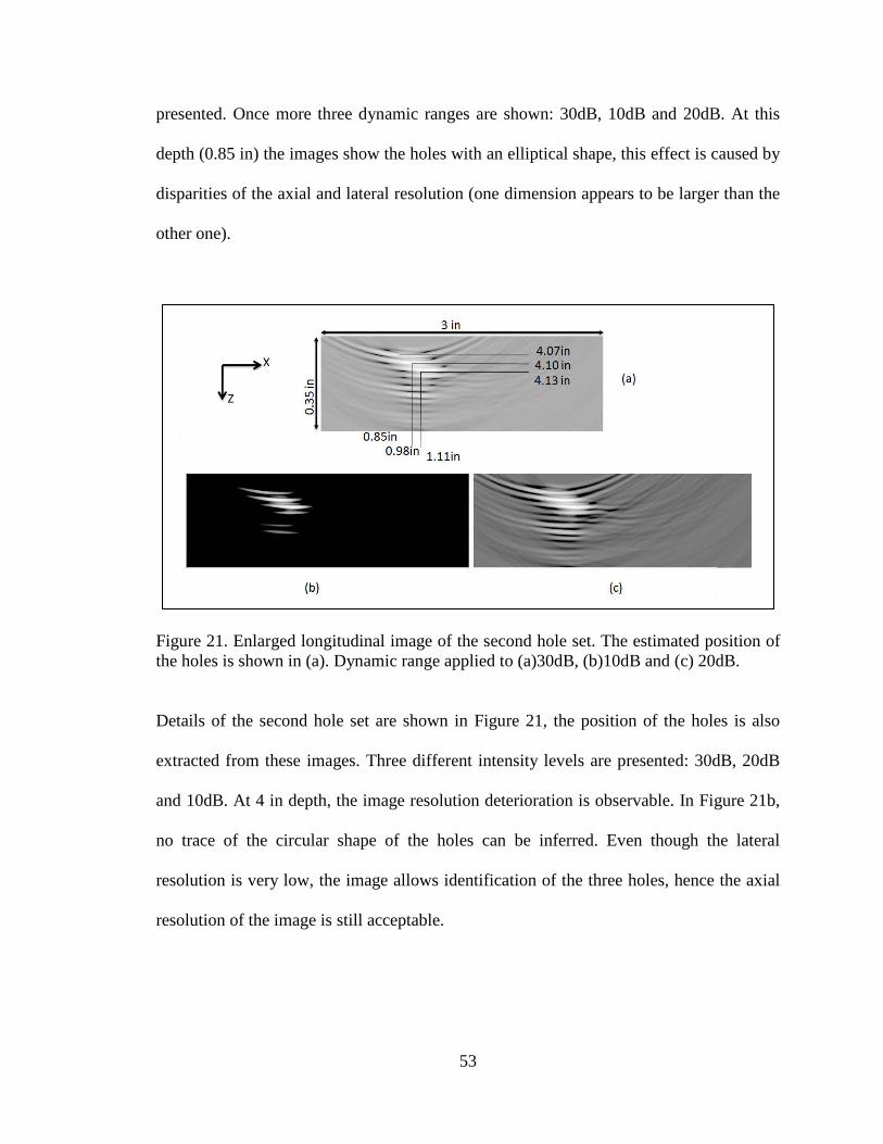
53

presented. Once more three dynamic ranges are shown: 30dB, 10dB and 20dB. At this

depth (0.85 in) the images show the holes with an elliptical shape, this effect is caused by

disparities of the axial and lateral resolution (one dimension appears to be larger than the

other one).

Figure 21. Enlarged longitudinal image of the second hole set. The estimated position of the holes is shown in (a). Dynamic range applied to (a)30dB, (b)10dB and (c) 20dB.

Details of the second hole set are shown in Figure 21, the position of the holes is also

extracted from these images. Three different intensity levels are presented: 30dB, 20dB

and 10dB. At 4 in depth, the image resolution deterioration is observable. In Figure 21b,

no trace of the circular shape of the holes can be inferred. Even though the lateral

resolution is very low, the image allows identification of the three holes, hence the axial

resolution of the image is still acceptable.

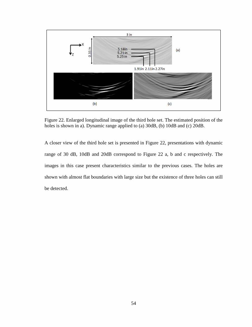
54

Figure 22. Enlarged longitudinal image of the third hole set. The estimated position of the holes is shown in a). Dynamic range applied to (a) 30dB, (b) 10dB and (c) 20dB.

A closer view of the third hole set is presented in Figure 22, presentations with dynamic

range of 30 dB, 10dB and 20dB correspond to Figure 22 a, b and c respectively. The

images in this case present characteristics similar to the previous cases. The holes are

shown with almost flat boundaries with large size but the existence of three holes can still

be detected.

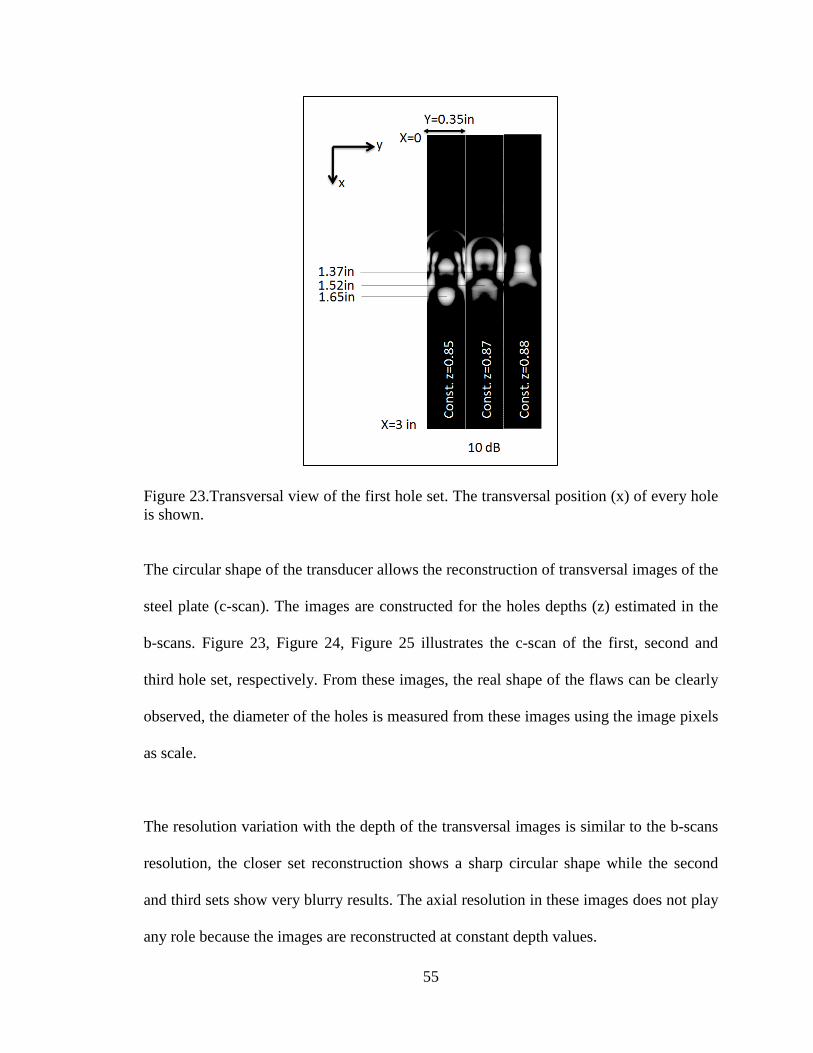
55

Figure 23.Transversal view of the first hole set. The transversal position (x) of every hole is shown.

The circular shape of the transducer allows the reconstruction of transversal images of the

steel plate (c-scan). The images are constructed for the holes depths (z) estimated in the

b-scans. Figure 23, Figure 24, Figure 25 illustrates the c-scan of the first, second and

third hole set, respectively. From these images, the real shape of the flaws can be clearly

observed, the diameter of the holes is measured from these images using the image pixels

as scale.

The resolution variation with the depth of the transversal images is similar to the b-scans

resolution, the closer set reconstruction shows a sharp circular shape while the second

and third sets show very blurry results. The axial resolution in these images does not play

any role because the images are reconstructed at constant depth values.

56

Figure 24. Transversal view of the second hole set. The transversal position (x) of every hole is shown.

Figure 25. Transversal view of the third hole set. The transversal position (x) of every hole is shown.

57

Figure 26. Combination of longitudinal and transversal images of a 1018 steel plate using synthetic phased array imaging technique.

The final image, Figure 26, shows a combination of a b-scan and c-scan for the first hole

set. These combination present very precise details of the holes, diameter and position

can be clearly identified. A comparison between the position obtained from the images

and the real hole position is summarized in Table 2. In general the errors obtained are

below 7%, but as expected higher errors are obtained in the transversal position

estimation due to the lower lateral resolution. In addition the horizontal position of the

holes is calculated relative to the array position, hence some error can be attributed to the

initial array positioning.

58

Table 2. Real and obtained positions of the machined holes. X position (in) (Exp/Real) Y position (in) (Exp/Real)

Hole Set #1

1.38/1.34 0.85/0.85

1.5/1.55 0.86/0.869

1.65/1.66 0.88/0.884

Hole Set #2

0.85/0.727 4.07/4.127

0.98/0.880 4.10/4.154

1.11/1.035 4.13/4.180

Hole Set #3

1.91/1.823 5.18/5.31

2.11/1.974 5.21/5.27

2.27/2.124 5.25/5.23

The error associated with the longitudinal position (y) does not have any influence from

the array position. The errors in the longitudinal position error are summarized in Table

3. It is noticeable that the maximum error is only 2.45% within a depth of five inches. At

the closer hole locations, the errors are much lower, inaccuracies of 0.02cm and less are

found. The second hole set has errors of less than 1.5%, which is less than 0.15cm of

disparity, so the imaging system shows a high longitudinal resolution even at big depths.

59

Table 3. Error associated with the longitudinal position estimation based in the acoustic images.

y position Error(in) y position error (cm) y position Error(%)

Hole Set #1

0 0.00 0.00%

0.009 0.02 1.03%

0.004 0.01 0.45%

Hole Set #2

0.057 0.14 1.38%

0.054 0.14 1.30%

0.05 0.13 1.20%

Hole Set #3

0.13 0.33 2.45%

0.06 0.15 1.14%

0.02 0.05 0.38%

3.4 Chapter Review and Conclusions

In section 3.1 an experimental setup for SAW velocity calculation is presented and

explained. The waves are created in a 1018 steel plate that is used in future experiments;

the estimated velocity is compared with the theoretical value calculated with the classical

SAW velocity formulation [60]. The difference in the estimated and calculated velocity is

so small (1.2%) that either of those can be used for future experimentation with minimal

error. The section 3.2 also presents a methodology for estimation of an important acoustic

material property of the 1018 steel plate: the attenuation coefficient. A series of SAW

reflections acquired at different positions help to measure the intensity changes of the

waves while they propagate through the plate. The experiment results confirm the

60

exponential behavior of the wave attenuation and deliver the attenuation coefficient,

parameter that is used in the experiments presented in chapter 4.

Finally in section 3.3, the conventional synthetic array imaging technique is tested.

Estimation of artificial flaws in a 1018 steel plate is performed through a 5MHz

transducer with 1/2in of circular aperture and a synthetic array of 55 elements and 0.1in

of elementary pitch. While at depths of 0.85in the reconstructed images still show

acceptable resolution, at depths superior to 4in the attenuation and diffraction deteriorates

the lateral resolution of the images significantly. Although the attenuation also affects the

longitudinal resolution, the effect of it is less severe; at depths up to 4in the position error

is inferior to 1.5% while at 5in the error increases to around 2.5%. This imaging system

has proved to have good accuracy in the estimation of the longitudinal position of small

objects at different depths, hence it can be employed in the experiments of Chapter 4

.

61

CHAPTER 4: BOLT TENSION ESTIMATION USING SURFACE ACOUSTIC

WAVES

4.1 Conceptual Framework

A novel methodology for detection of tension in bolted joints using surface acoustic

waves (SAW) is presented. Surface acoustic waves are used to estimate changes in the

area of real contact created in-between the bolt head and the clamped elements. As it was

explained in chapter 1, the increment of the bolt tension creates an expansion of the real

area of contact (RAC), hence estimation of changes in the RAC lead to assessment of the

bolt tension. In Figure 27 a schematic presentation of the method can be observed. A

crystal wedge is used to generate SAW in a metal plate towards a previously tensioned ¼

inch bolt.

Figure 27. Schematic set up of the proposed methodology.

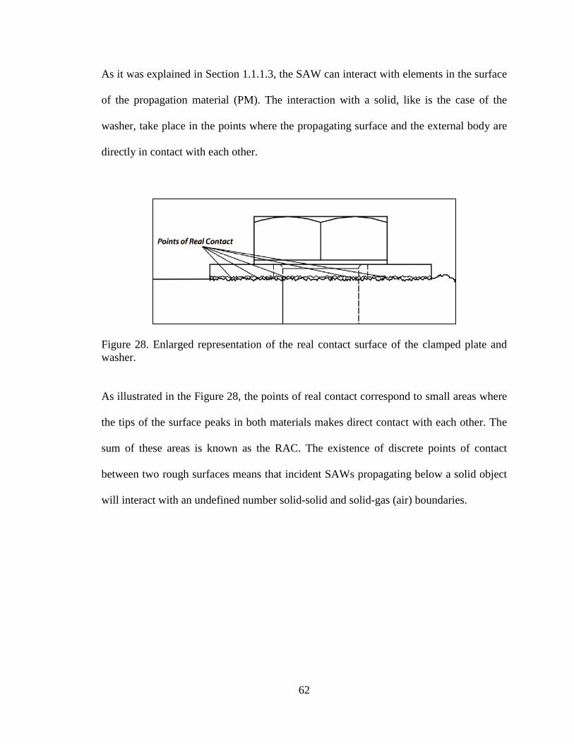
62

As it was explained in Section 1.1.1.3, the SAW can interact with elements in the surface

of the propagation material (PM). The interaction with a solid, like is the case of the

washer, take place in the points where the propagating surface and the external body are

directly in contact with each other.

Figure 28. Enlarged representation of the real contact surface of the clamped plate and washer.

As illustrated in the Figure 28, the points of real contact correspond to small areas where

the tips of the surface peaks in both materials makes direct contact with each other. The

sum of these areas is known as the RAC. The existence of discrete points of contact

between two rough surfaces means that incident SAWs propagating below a solid object

will interact with an undefined number solid-solid and solid-gas (air) boundaries.

63

Figure 29. Schematic representation of change in the RAC due to tension increments.

Increasing the tension in the bolt raises the number and the size of reflection points

(points of contact). Figure 29 illustrates a schematic representation of the RAC growth

due to increments in bolt tension. The RAC is different from the apparent area of

contact, but at high tension levels the difference between those is minimal [61]. The

saturation of the RAC at some preload level establishes the maximum tension level that

can be measured with the investigated concept.

The way in which the RAC expands is of special interest for tension estimation. The

RAC grows from the washer center to the washer perimeter, as illustrated in Figure 29.

This behavior can be explained by analyzing the way in which the tension is applied to

the bolt head: the preload transforms into a pulling force exerted in the head center, hence

64

the surface peaks closer to it are expect to be more affected than the ones in the perimeter

and therefor a radial expansion of the RAC can be predicted. This growth trend means

that SAW face an acoustic wall that approaches to wedge as the preload is increased.

Figure 30. Representation of SAW reflection from 4 different boundaries. White arrows represent no load, green arrows low load, blue arrows medium load and red arrows high load. The black arrows represent the incoming SAW.

The change in position of the acoustic wall denotes a change in the tension applied to the

bolt head. An acoustic wall is a series of the points where free movement of the waves is

constrained e.g. the contact points of two solid objects. Material discontinuities, holes and

object edges also behave as acoustic walls. In Figure 30 a schematic representation of the

SAW reflection from different acoustics barriers is illustrated. The colored arrows denote

the main reflection of the incoming SAW (black arrows). The RAC find its minimum

65

value when the bolt has no tension, in this case the main reflections come from the plate

hole (white arrows). As the load is increased and the RAC grows, the main reflections

move from the hole boundary and get closer to the washer perimeter. Figure 30 illustrates

the reflection of 4 different states, no load (white), low load (green), medium load (blue)

and high load (red). The changes in position of the acoustic wall are represented by a

delay in the received wave, which means that every preload value has a related wall

position represented by a specific time of flight (TOF) of the reflected waves. A

relationship TOF vs. bolt tension can be generated.

In the following experiments the explained concept is tested. A plate of steel is used as

the propagating material, bolts of 1/4in and 1/2 in are tensioned with different torque

levels and the changes in the RAC are monitored. The RAC changes are inspected with

the conventional synthetic phased array imaging technique. The images permit to

establish the exact position of the acoustic wall created by the contact of the bolt head

and the plate surface.

4.2 Tension Evaluation of a 1/4in Stainless Steel Bolt

In this study the proposed methodology is tested with a stainless steel bolt of 1/4in

diameter installed in a 1018 steel plate. As the RAC growth affects the position of the

SAW main reflections, it is necessary to establish very precisely where those reflections

take place. In chapter 3 a synthetic phased array imaging method is used to find the

location of very small holes in a steel plate. The reconstructed images presented very

good longitudinal resolution, consequently the same imaging system is used in the

experiments of this chapter.

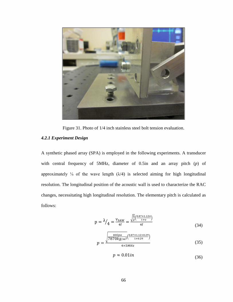
66

Figure 31. Photo of 1/4 inch stainless steel bolt tension evaluation.


A synthetic phased array (SPA) is employed in the following experiments. A transducer

with central frequency of 5MHz, diameter of 0.5in and an array pitch (p) of

approximately ¼ of the wave length (λ/4) is selected aiming for high longitudinal

resolution. The longitudinal position of the acoustic wall is used to characterize the RAC

changes, necessitating high longitudinal resolution. The elementary pitch is calculated as

follows:

p = λ4 = VSAW

4f=

Gρ0.87+1.12υ

1+υ

4f

𝑝 =

80𝐺𝑝𝑎7870𝑘𝑔/𝑚2

0.87+1.12×0.291+0.29

4×5𝑀𝐻𝑧

𝑝 ≈ 0.01𝑖𝑛

(34)

(35)

(36)

67

Where f is the transducer center frequency, G, ν, ρ are respectively the shear modulus, the

Poisson’s ratio and the density of the 1018 steel. Properties were taken from [57].

The number of elements in the array (NE) determines the array aperture (length) which is

proportional to the lateral resolution. Therefore high number of elements increases the

resolution, at a cost of increasing scanning time, so a balance between image quality and

experiment duration should be determined. In this study, it was decided to create and

array of 50 elements, so the array has an active aperture of 0.5in.

In addition to the array aperture, the distance to the target also affects the image lateral

resolution. The best resolution is achieved with a separation equal to the transducer

natural focus (NF). As discussed in section 1.1.2, the NF is the point of maximum

transverse relative intensity within the focal area. The NF position (N) is calculated with

the formulation presented in section 1.1.2, but due to the presence of the wedge, the

distance to the target (AP) is founded by subtracting the space inside the wedge (1.7in):

AP = N − 1.7in = D2f4c− 1.7𝑖𝑛

𝐴𝑃 = 0.5𝑖𝑛2×5𝑀𝐻𝑧4×2953𝑚/𝑠

− 1.7𝑖𝑛

𝐴𝑃 = 1.0 𝑖𝑛

Where D is the transducer diameter, f the transducer’s center frequency, c is the SAW

speed in 1018 steel, NF is the transducer’s natural focus and AP the array position with

respect to the bolt. Figure 32 illustrates a sketch of the final configuration.

(37)

(38)

(39)

68

Figure 32. Sketch of transducer-wedge position with respect to the targeted hole.

Stretching the bolt increases the bolt tension and hence increasing the RAC between the

bolt head and the steel plate. It discussed previously the RAC and the normal force are

proportional [61]. The bolt tension is equivalent to the normal force in this application:

The elongation of the bolt body creates a pulling force at the bolt head, but is also the

deformation in the bolt body which creates the tension force. In this sense, the tension

force pulls the bolt head against the plate in the same as the normal force would push it.

In this experiment the bolt tension is not directly controlled but the torque applied to the

bolt is controlled. In chapter 1 it was explained that torque and tension are related by the

bolt diameter and a friction factor which is a function of screw type and the materials in

contact. From this perspective, for a particular bolt installed in a specific plate, the torque

and tension are proportional in nature. As a result, the torque and RAC values are also

proportional:

(40)

69

𝑇 ∝ 𝐹𝑁 ∧ RAC ∝ 𝐹𝑁

Then

RAC ∝ 𝑇

Where T is the torque applied to the bolt, FN is the normal force and RAC is the real area

of contact.

One can infer from this equation that the RAC can be adjusted by controlling the specific

amount of torque applied to the bolt. In this first set of experiment conducted, three

torque levels are applied: no torque, medium torque and maximum torque.


There are three key components in the experiment setup: precise position controlling

system, SAW generation system and the bolted joint. The position control of the

transducer-wedge attachment is achieved through a manual translator stage with

resolution of 0.001in and maximum displacement span of 1in. The transducer and the

wedge are adapted to the translator stage (Thorlabs PT3) by specially designed aluminum

parts.

The electronic signals are generated and received by a pulse generator (Olympus

5072PR) and an oscilloscope (Tektronix TDS 2024B). A 5MHz piezoelectric transducer

(PZT) with circular aperture of 1/2in is driven by the pulse generator. A crystal wedge is

attached to the PZT for creating SAW in the steel plate. The configuration of the devices

is presented in Table 4.

(41)

70

Table 4. Parameters employed in the experimental configuration of section 4.2. Pulse generator Damping 50Ω

Pulse generator PRF 200 Hz

Amplification 45dB

Pulse generator LPF (1MHz) ON

Pulse Generator HPF (10MHz) ON

SAW velocity 2590 m/s

Transducer Frequency 5 MHz

Transducer Diameter 0.5 in

Array Pitch (in) 0.01 in

Number of Elements 50

Target Distance 2.7 in

Bolt Diameter 0.5in

The bolted joint employ in this test is formed by a 1018 steel plate and a ¼ in 20UNC

bolt. Neither nut nor washer is used in this test. The bolt is tightened with help of the

threaded holes present in the work bench (Figure 31). In Figure 33 dimension and

characteristics of the machined holes are illustrated. It is important to notice that all the

holes in the plate have a coarse thread. This characteristic facilitates the installation of the

tested bolts. Additionally, no lubricant is used in the joint. The surface conditions of the

threads are good enough to permit proper bolt tightening. The plate can be attached to the

work bench by C-clamps when is so required. Additional information about the devices

employed is presented in Appendix A.

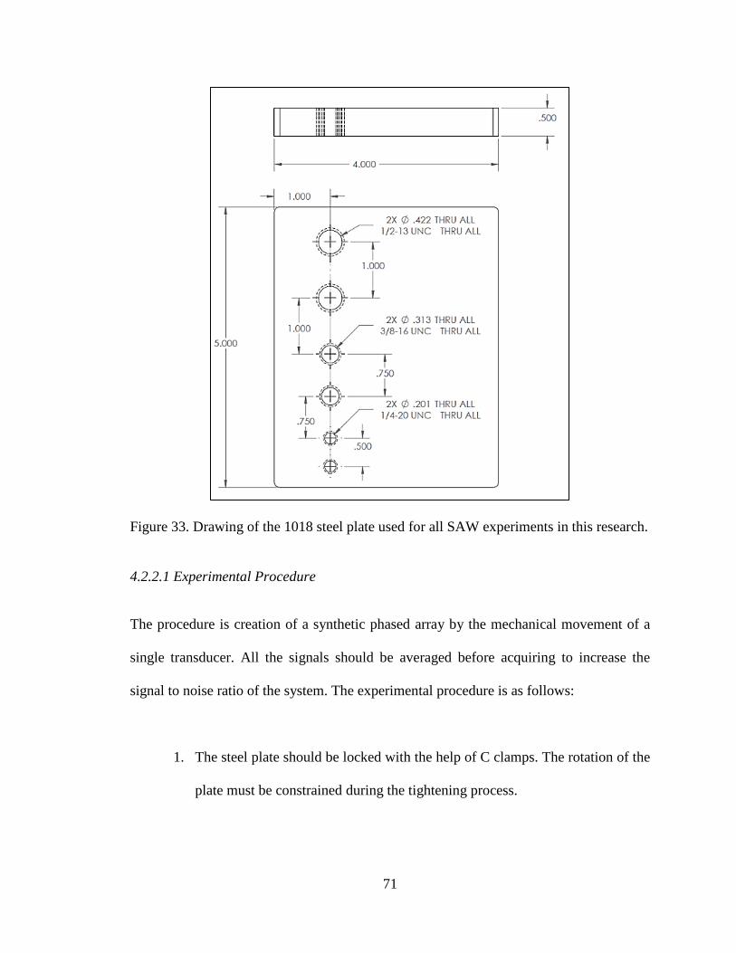
71

Figure 33. Drawing of the 1018 steel plate used for all SAW experiments in this research.


The procedure is creation of a synthetic phased array by the mechanical movement of a

single transducer. All the signals should be averaged before acquiring to increase the

signal to noise ratio of the system. The experimental procedure is as follows:

1. The steel plate should be locked with the help of C clamps. The rotation of the

plate must be constrained during the tightening process.

72


aluminum L and aluminum plate. The height of this assembly must permit the




waves.

3. The TS is employed to position the wedge as is shown in Figure 32. It is very

helpful to use the steel plate edges as reference. The movement span of the TS

is only one inch, so the positioning process should take into account that the

wedge needs to move 0.5in after initially positioned.





5. In order to start the recording process, the signal recording mode should be set

to average; this helps to increase the signal to noise ratio of the system. After

recording the signal at the initial point, the transducer should be moved 0.01in

to the right; prior to recording the second response, the average function

should be reset. This procedure is repeated until 50 data are collected.

73

6. After the first 50 data are collected, the bolt should be installed and tightened

with a wrench until a medium torque value is achieved. This is the starting

point for a new set of 50 data. Before the third data set is recorded the bolt

should be tightened up again.


The imaging reconstruction generates three images correspondent to the applied torque

levels. Figure 34 illustrates the results as 15dB of dynamic range. The array is located at

the left of the image. In the center of the images, the reflections from the bolt head are

clearly distinguishable.

Figure 34. Generated images of the steel plate at 15dB of dynamic range. Applied torque a) none, b) medium and c) maximum.

a)

b)

c)

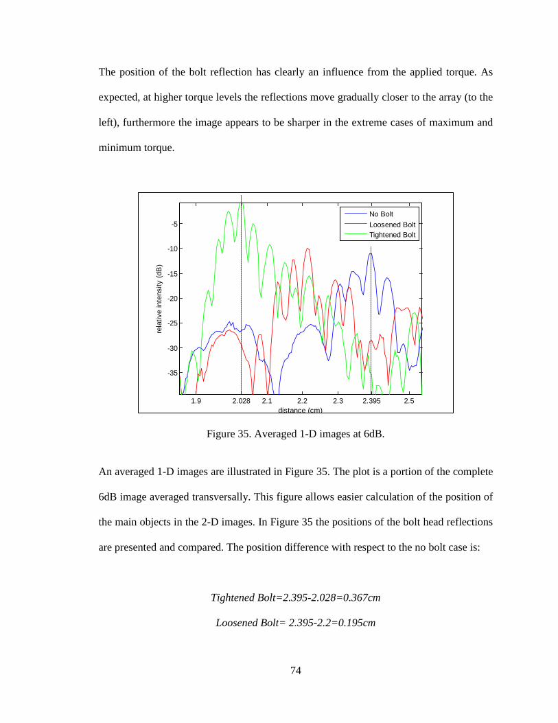
74

The position of the bolt reflection has clearly an influence from the applied torque. As

expected, at higher torque levels the reflections move gradually closer to the array (to the

left), furthermore the image appears to be sharper in the extreme cases of maximum and

minimum torque.

Figure 35. Averaged 1-D images at 6dB.

An averaged 1-D images are illustrated in Figure 35. The plot is a portion of the complete

6dB image averaged transversally. This figure allows easier calculation of the position of

the main objects in the 2-D images. In Figure 35 the positions of the bolt head reflections

are presented and compared. The position difference with respect to the no bolt case is:

Tightened Bolt=2.395-2.028=0.367cm

Loosened Bolt= 2.395-2.2=0.195cm

1.9 2.028 2.1 2.2 2.3 2.395 2.5

-35

-30

-25

-20

-15

-10

-5

distance (cm)

rela

tive

inte

nsity

(dB

)

No BoltLoosened BoltTightened Bolt

75

4.3 Tension Evaluation of a 1/2in Stainless Steel Bolt

This experiment tests the proposed concept with a 1/2inch 13UNC stainless steel bolt.

The larger bolt allows the application of higher tension levels, it also increases the

geometric area of contact, and hence larger changes in the RAC are expected.

Additionally this bolt size is more representative of a civil structure, which is the possible

future application of the methodology.

Figure 36. Photo of ½ inch stainless steel bolt tension evaluation.

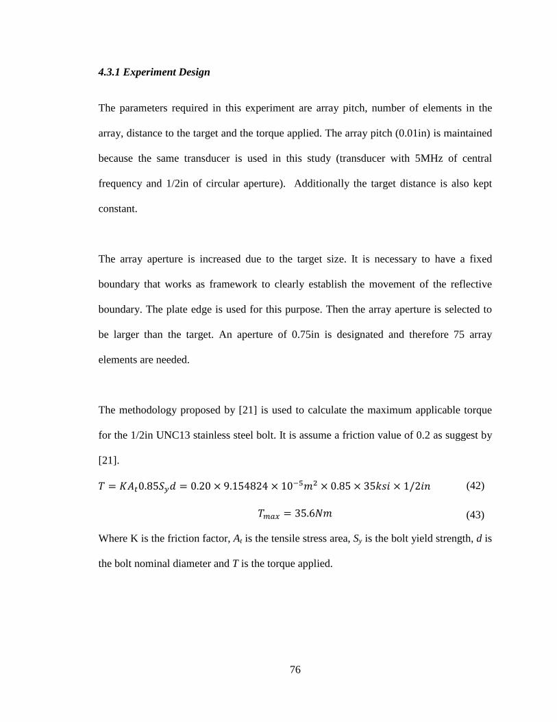
76


The parameters required in this experiment are array pitch, number of elements in the

array, distance to the target and the torque applied. The array pitch (0.01in) is maintained

because the same transducer is used in this study (transducer with 5MHz of central

frequency and 1/2in of circular aperture). Additionally the target distance is also kept

constant.

The array aperture is increased due to the target size. It is necessary to have a fixed

boundary that works as framework to clearly establish the movement of the reflective

boundary. The plate edge is used for this purpose. Then the array aperture is selected to

be larger than the target. An aperture of 0.75in is designated and therefore 75 array

elements are needed.

The methodology proposed by [21] is used to calculate the maximum applicable torque

for the 1/2in UNC13 stainless steel bolt. It is assume a friction value of 0.2 as suggest by

[21].

𝑇 = 𝐾𝐴𝑡0.85𝑆𝑦𝑑 = 0.20 × 9.154824 × 10−5𝑚2 × 0.85 × 35𝑘𝑠𝑖 × 1/2𝑖𝑛

𝑇𝑚𝑎𝑥 = 35.6𝑁𝑚

Where K is the friction factor, At is the tensile stress area, Sy is the bolt yield strength, d is

the bolt nominal diameter and T is the torque applied.

(42)

(43)

77

The analysis of the experiments in this thesis is performed using the changes of the

parameters of interest: tension, torque and boundary position. Therefore the uncertainties

in the tension applied to the bolt, which depends of the friction and may vary up to 50%

[62], do not affect the result analysis. As explained in section 4.2.1 that RAC, tension and

torque are proportional in nature, hence the proportionality coefficients, like the friction

in the case of torque-tension, influence the value of the parameters but not the changes

produced by them.

The maximum torque is higher than the supported by the torque wrench, so the maximum

torque supported by the wrench is chosen. Additionally due to the high number of array

elements, the torque states were decided to be three.


𝑇𝑖𝑛𝑐𝑟𝑒𝑚𝑒𝑛𝑡𝑠 = 𝑇𝑚𝑎𝑥3

≈ 15.48𝑁𝑚


The position controlling system, SAW generation system are the same as the ones

discussed in the prior section. The translator stage (Thorlabs PT3), the pulse generator

(Olympus 5072PR) and the oscilloscope (Tektronix TDS 2024B) are also employed in

this experiment. The 1018 steel plate is also kept but the 1/2in threaded hole is used this

time. The tested bolt is a 1/2in 13UNC stainless steel bolt. In this experiment the

workbench cannot be used to tighten the bolt due to the size difference, hence a ½ inch

stainless steel nut is employed for this purpose. It is not necessary to apply lubrication in

this case neither. The configuration of all the devices is presented in Table 5.

(44)

(45)

78

Table 5. Parameters employed in the experimental configuration of section 4.3.Pulse generator

Damping

50Ω


Amplification 45dB

Pulser LPF & HPF ON


Transducer

Frequency

5 MHz





Bolt Diameter 0.5in

Bolt Yield Strength 35 ksi

Friction Factor 0.20

Tensile Stress Area 9.154824x

10-5m2

Maximum Torque 29.03 Nm

Torque Increments 15.48Nm


1. The steel plate should be locked with help of C clamps. The rotation of the







waves.

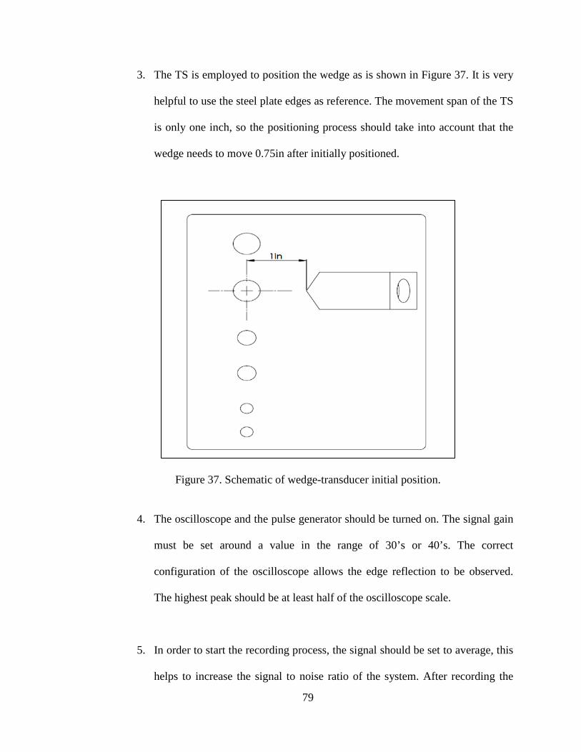
79

3. The TS is employed to position the wedge as is shown in Figure 37. It is very




Figure 37. Schematic of wedge-transducer initial position.







80



This procedure is repeated until 75 data are collected.

6. After the first 75 data are collected the bolt should be tightened with the

torque wrench until 15.48 Nm are reached. This is the starting point for a new

set of 75 data. Following the torque should be increased up to the maximum

value supported by the wrench (29.03Nm).


One image at every torque value is constructed. In Figure 38 the results are presented at

15dB of dynamic range. In the images the clear reflection from the hole and the nut can

be observed, but the position variation in not clear.

Figure 38. Generated images of the steel plate at 15dB of dynamic range.

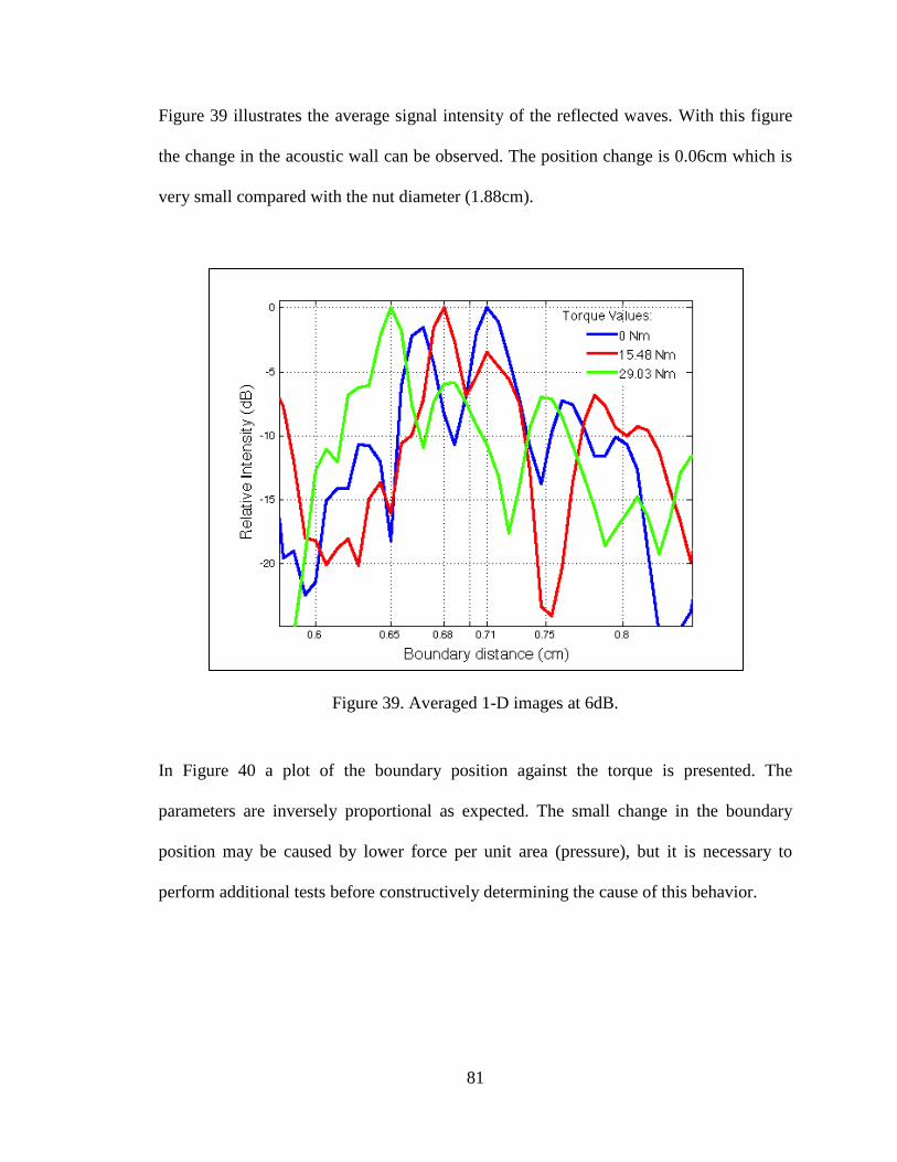
81

Figure 39 illustrates the average signal intensity of the reflected waves. With this figure

the change in the acoustic wall can be observed. The position change is 0.06cm which is

very small compared with the nut diameter (1.88cm).


In Figure 40 a plot of the boundary position against the torque is presented. The

parameters are inversely proportional as expected. The small change in the boundary

position may be caused by lower force per unit area (pressure), but it is necessary to

perform additional tests before constructively determining the cause of this behavior.

82

Figure 40. Plot of torque applied versus position of the acoustic wall.

4.4 Tension Evaluation of a 1/4in Grade 8 Bolt

In this experiment higher tension levels are tested. In the set of experiment of section 4.2

the mechanical resistance of the stainless steel bolt prevents further increments of the

torque levels therefore in this occasion a 1/4in grade 8 bolt is employed. Grade 8 bolts

have yield strength almost 3 times higher than stainless steel bolts [57].Additionally a

stainless steel washer is fixed to the bolt in order to increase the expansion capability of

the RAC (Figure 41).

0 5 10 15.48 20 25 29.030.64

0.65

0.66

0.67

0.68

0.69

0.7

0.71

0.72

Torque (Nm)

Bou

ndar

y di

stan

ce (c

m)

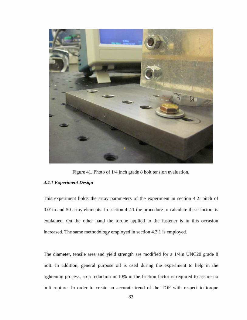
83

Figure 41. Photo of 1/4 inch grade 8 bolt tension evaluation.


This experiment holds the array parameters of the experiment in section 4.2: pitch of

0.01in and 50 array elements. In section 4.2.1 the procedure to calculate these factors is

explained. On the other hand the torque applied to the fastener is in this occasion

increased. The same methodology employed in section 4.3.1 is employed.

The diameter, tensile area and yield strength are modified for a 1/4in UNC20 grade 8

bolt. In addition, general purpose oil is used during the experiment to help in the

tightening process, so a reduction in 10% in the friction factor is required to assure no

bolt rupture. In order to create an accurate trend of the TOF with respect to torque

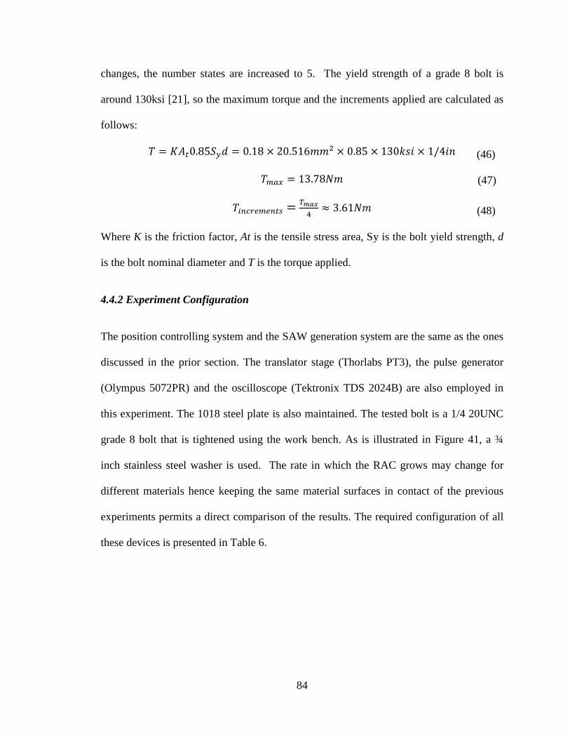
84

changes, the number states are increased to 5. The yield strength of a grade 8 bolt is

around 130ksi [21], so the maximum torque and the increments applied are calculated as

follows:

𝑇 = 𝐾𝐴𝑡0.85𝑆𝑦𝑑 = 0.18 × 20.516𝑚𝑚2 × 0.85 × 130𝑘𝑠𝑖 × 1/4𝑖𝑛


𝑇𝑖𝑛𝑐𝑟𝑒𝑚𝑒𝑛𝑡𝑠 = 𝑇𝑚𝑎𝑥4

≈ 3.61𝑁𝑚

Where K is the friction factor, At is the tensile stress area, Sy is the bolt yield strength, d

is the bolt nominal diameter and T is the torque applied.


The position controlling system and the SAW generation system are the same as the ones

discussed in the prior section. The translator stage (Thorlabs PT3), the pulse generator

(Olympus 5072PR) and the oscilloscope (Tektronix TDS 2024B) are also employed in

this experiment. The 1018 steel plate is also maintained. The tested bolt is a 1/4 20UNC

grade 8 bolt that is tightened using the work bench. As is illustrated in Figure 41, a ¾

inch stainless steel washer is used. The rate in which the RAC grows may change for

different materials hence keeping the same material surfaces in contact of the previous

experiments permits a direct comparison of the results. The required configuration of all

these devices is presented in Table 6.

(46)

(47)

(48)

85

Table 6. Parameters employed in the experimental configuration of section 4.4. Pulse generator

Damping 50Ω


Amplification 45dB

Pulse generator LPF

(1MHz) ON

Pulse Generator HPF

(10MHz) ON


Transducer Frequency 5 MHz





Bolt Diameter 0.25 in

Bolt Yield Strength 130 ksi

Friction Factor 0.18

Tensile Stress Area 20.516 mm2

Maximum Torque 17.86 Nm

Torque Increments 3.61Nm


1. The steel plate should be locked with help of C clamps. The rotation of the







waves.

86

3. The TS is employed to position the wedge as is shown in Figure 42 It is very




Figure 42. Schematic of the wedge initial position.









This procedure is repeated until 50 data are collected.

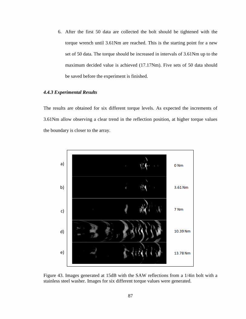
87

6. After the first 50 data are collected the bolt should be tightened with the

torque wrench until 3.61Nm are reached. This is the starting point for a new

set of 50 data. The torque should be increased in intervals of 3.61Nm up to the

maximum decided value is achieved (17.17Nm). Five sets of 50 data should

be saved before the experiment is finished.


The results are obtained for six different torque levels. As expected the increments of

3.61Nm allow observing a clear trend in the reflection position, at higher torque values

the boundary is closer to the array.

Figure 43. Images generated at 15dB with the SAW reflections from a 1/4in bolt with a stainless steel washer. Images for six different torque values were generated.

a)

b)

c)

d)

e)

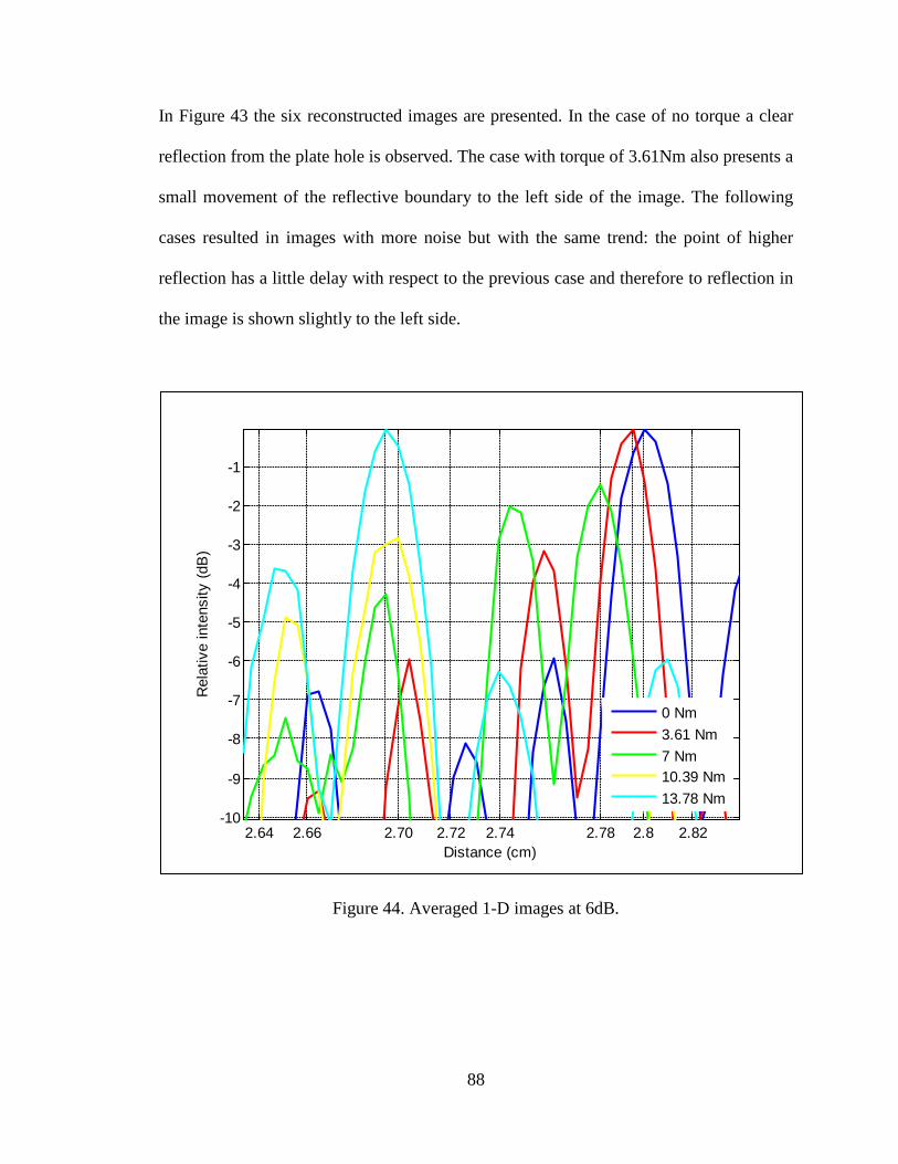
88

In Figure 43 the six reconstructed images are presented. In the case of no torque a clear

reflection from the plate hole is observed. The case with torque of 3.61Nm also presents a

small movement of the reflective boundary to the left side of the image. The following

cases resulted in images with more noise but with the same trend: the point of higher

reflection has a little delay with respect to the previous case and therefore to reflection in

the image is shown slightly to the left side.


2.64 2.66 2.70 2.72 2.74 2.78 2.8 2.82-10

-9

-8

-7

-6

-5

-4

-3

-2

-1

Distance (cm)

Rel

ativ

e in

tens

ity (d

B)

0 Nm3.61 Nm7 Nm10.39 Nm13.78 Nm

89

The change in the position of the main reflection is exposed clearly in Figure 44. The

maximum points of maximum average signal intensity are plotted against its position in

the images. It can be easily observed that the maximum intensity point of the blue signal

(0 Nm) is separated from the peak of the light blue signal (13.78 Nm) approximately by

0.1cm. The remaining signal peaks are located between these extreme values.

Figure 45. Graph of the torque applied versus the position of the acoustic wall.

The Figure 45 illustrates the change in distance product of torque variation. A reduction

of 0.11cm in the boundary separation is founded as the torque is increased from 0 to

13.78 Nm. The position changes do not correspond linearly to the torque increments, as

can be observed in Figure 45. This behavior can be explained by the fact that the RAC is

not directly measured, only the size of the characteristic length may be estimated with the

image. Then the boundary distance and the torque are not expected to be linear.

0 2 3.61 6 7 10.39 13.782.68

2.7

2.72

2.74

2.76

2.78

2.8

2.82

Torque (Nm)

Dis

tanc

e (c

m)

90

Another important characteristic of the plot is the apparent RAC saturation taking place

at 10.39 Nm. The saturation phenomenon is explained in detail section 4.1. Apparently,

the maximum RAC is achieved at a boundary position of around 2.7cm, but the washer

edge is located at 3.335cm (The washer radius is 0.635cm). This behavior can be

explained by the bending suffered by the washer, which influences the growth of the

RAC.

4.4.4 Error Estimation

4.4.4.1 Signal to Noise Ratio of the System

In order to analyze the error associated with the generated images, it is necesarry to

measure the signal to noise ratio (SNR) of the received signals(a-scans). In

Figure 46 the SNRs of the signals reflected by the bolt are presented. The graph

illustrates the SNR levels for the 50 signals correspondent to every position of the

transducer. As expected the SNR increase in the center signals due to the reflection from

the washer (or the hole). It can also be noticed that the average SNR decrases as the

torque level is increased, which means that the quality of the images produced at the

higher torque levels is lower than in the lower torque states. Lower image quality lead to

unacuarate estimation and greater error. The minimum dynamic range that can be

applied to the images is determined by the averaged SNR.

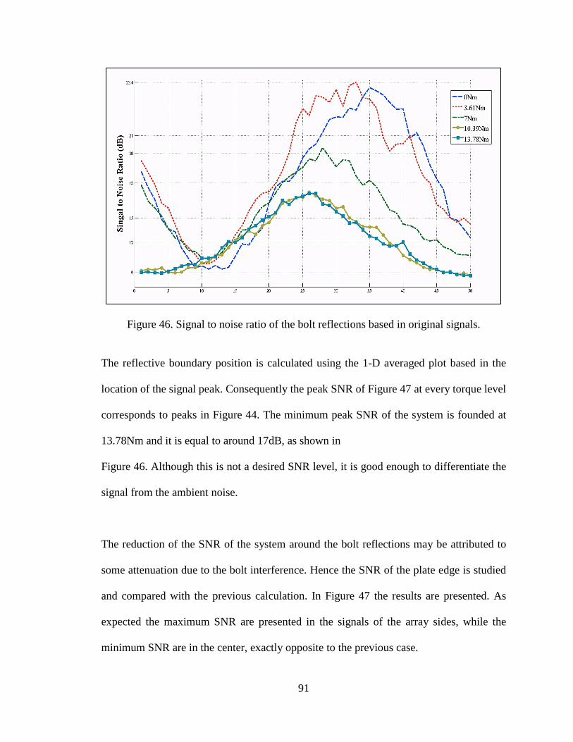
91

Figure 46. Signal to noise ratio of the bolt reflections based in original signals.

The reflective boundary position is calculated using the 1-D averaged plot based in the

location of the signal peak. Consequently the peak SNR of Figure 47 at every torque level

corresponds to peaks in Figure 44. The minimum peak SNR of the system is founded at

13.78Nm and it is equal to around 17dB, as shown in

Figure 46. Although this is not a desired SNR level, it is good enough to differentiate the

signal from the ambient noise.

The reduction of the SNR of the system around the bolt reflections may be attributed to

some attenuation due to the bolt interference. Hence the SNR of the plate edge is studied

and compared with the previous calculation. In Figure 47 the results are presented. As

expected the maximum SNR are presented in the signals of the array sides, while the

minimum SNR are in the center, exactly opposite to the previous case.

92

Figure 47. Signal to noise ratio of the plate edge reflections based in original signals

In the case of the plate edge, the behavior of the SNR peaks is not as clear as in the case

of the bolt reflections. With the intention of comparing them, a graph of the averaged

SNR for both cases is presented in Figure 48. Even though the signal loss tends to reduce

the SNR for both cases as the torque is increased, there is an abrupt SNR drop in the bolt

case. It is especially notorious when the torque is increased from 3.61Nm to 10.39Nm

and the SNR decrease from 18dB to 12dB.

93

Figure 48. Averaged signal to noise ratio of the bolt and plate edge reflections based in original signals.

This analysis permits to identify the existence of error sources that generate signal losses,

which finally reduce the SNR of the system. For instance, the acoustic couplant can be

inducing signal loss as the experiment is performed. The necessity to move the transducer

with the couplant may be causing that traces of gel interfere with the wave propagation.

Additionally the movement in the set up caused by the tightening process may cause

signal reduction.

As it was previously mentioned, there is more SNR reduction in the bolt surroundings

than in the plate edge when the torque is increased. This phenomenon is caused either by

sources of signal loss that only act in around the bolt or by signal attenuation due to the

increased tension. Additional experimentation should be performed in order to clarify this

behavior.

0 3.61 7 10.39 13.7810

12

14

16

18

20

22

24

26

Torque Level (Nm)

SNR

(dB)

Average SNR BoltAverage SNR Wall

94

4.4.4.2 Axial Resolution of the System

The axial resolution of the system permits to establish the accuracy of the system to

estimate the movement of the reflective boundary. In section 2.2.4.3 the axial resolution

was defined in equation 21. The frequency response and temporal pulse length of the

system are founded with a network analyzer. The resulted axial resolution of the system

is:

∆𝑙 = 𝐶 𝑡𝑝2

= 2593𝑚/𝑠 5.55×10−7𝑠2

= 0.072𝑐𝑚

The axial resolution is close to half of the total change in the boundary position (0.1cm),

which means that the imaging system employed has the capability to measure the

boundary position changes with enough accuracy. Although the axial resolution is

sufficient, a system with smaller axial resolution can achieve more accurate results that

permit better analysis of the tension-boundary position relation.

4.4.4.3 Conclusions

The imaging system employed has the correct SNR and enough axial resolution for the

investigation of RAC changes due to bolt tension in a ¼ inch bolt. A minimum SNR peak

of 17 dB is founded at the maximum torque level, while a boundary movement of 0.1cm

is measured with an axial resolution of 0.07cm. Both cases shows that the accuracy of the

system is enough but not ideal for the analysis. In order to increase the precision of the

system higher frequency and higher damped transducers can be employed. Additionally a

phased array can increase considerably the SNR and it may limit the interferences of

acoustic couplant caused by the mechanical movement of the transducer.

(49)

95

CHAPTER 5: CONCLUSIONS AND FUTURE WORK

5.1 Conclusions

In this thesis a novel methodology for measuring bolt tension based in surface acoustic

waves (SAWs) is presented. A linear transducer array is employed for creating a variable

acoustic beam. The methodology has potential for local or remote inspection of bolted

joints. Additionally the direction variability of the acoustic beam enables monitoring of

several bolted joints simultaneously.

The tension is estimated using the reflection of SAWs created by the bolt head

interference. Increments in the bolt tension rise the points of interaction between the

waves the bolt head (real area of contact) and therefore the position of reflective

boundaries. The variations are estimated using the “conventional linear synthetic array”

imaging technique. A singular transducer is actuated from predefined positions in order

to produce an array of signals that are subsequently arranged and added to construct an

acoustic image.

96

Three sets of experiments are presented in this research for validating the proposed

concept: tension estimation of a ¼” stainless steel bolt, a ½” stainless steel bolt and

¼”grade 8 bolt. The tension is not directly measured nor applied to the bolt; instead

controlled torque is used to generate the changes in the real area of contact. The torque

and bolt tension produce equivalent effects in the real area of contact. Three figures

summarize the experimental results: 2-D image of the reflective objects in the scanned

surface, 1-D averaged plot of the images and plot of the torque applied versus position of

the reflective boundary.

The 2-D image is a representation of the signals received by the transducer. The lighter

colors represent reflection with higher intensity while darker with lower intensity. The

images allow visualization of the position where the highest reflections take place. In the

experiments, the reconstructed images illustrate a clear trend in the position of the

reflective boundary when the applied torque is changed. In all cases the torque

increments increase the real area of contact and therefore the position of the reflective

boundary. As expected, the real area of contact grew from the bolt head center to the

perimeter, which causes an effect of apparent movement of the boundary. The SAWs

reflections only interact with the outer boundary of the real area of contact and as it

grows, the position in which the interaction takes place moves towards the array location.

The 1-D average plot is a simplification of the 2-D image. Taking the average of lateral

dimension of the 2-D image the graph is created. The 1-D plot allows establishing the

exact position of the maximum intensity point of the 2-D image. The position of this

97

point is used to estimate the actual distance change of the reflective boundary. In all the

experiment, this plot illustrates the same trend found in the 2-D image: The boundary

moves towards the array as the torque is increased. The averaged 1-D plot also allows

relating the torque level to the actual boundary position, which is a way to measure the

bolt tension using this methodology.

The final outcome are plots of the boundary position versus the torque applied to the bolt.

The graphs illustrate the actual change in position produced by the variation in the torque.

The test performed to the 1/2in bolt presents an almost linear variation of the boundary

position with the torque. In the 1/4in grade 8 bolt the results indicate two regions within

the graph. The first region presents a non-linear behavior, while the second one is a

saturation region. The saturation region (presented at the highest torque values) is

characterized by slight changes in the boundary position due to torque increments.

The study proves the potential of the methodology for performing measurements of the

applied tension. It is concluded that the actual shape of the real area of contact is not yet

determined. While in the 1/2in bolt experiment, the relation torque-boundary position is

linear, in the 1/2in grade 8 bolt it is not. The shape of the real area of contact is different

for every experiment. The relation is expected to be a second grade polynomial. The area

changes are estimated with variations of a “characteristic length” therefore a square value

of the length should represent better the area changes. Finally, the saturation region

founded in the last experiment shows the frontiers of the sensing capacity of the system.

98

The presented experiments are the first steps towards the development of bolt tension

sensor based in surface acoustic waves. The results showed that the system has the

potential to inspect tension in bolts of ½ and ¼ inches. Further experimentation is needed

in order to better understand the behavior real area of contact and its interaction with the

SAWs.

5.2 Future Work

In order to increase the accuracy of the system, an array of transducers should be used for

the imaging generation. With the array configuration, the image quality will be improved

and the experimental time will be considerably reduced. Shorter experimental time will

allow the experimentation with more tension states and different kind of materials. A real

array of transducer will help to generate the images from different angles, which will

provide more information about the real area of contact.

Although the tension and torque levels presented in a specific bolt are expected to be

equivalent, the uncertainties associate with the friction may induce error in the tension

estimation. In order to reduce this drawback, a direct tension estimation methodology can

be employed. Load cells installed between the bolt head and the clamped plate can be

used to measure the tension applied to the bolt, which then can be compared with the

boundary position, just as it was done with the torque levels in this thesis.

99

The principal application of the methodology is the estimation of tension in threaded

fasteners, but the real area of contact can also be studied with this approach. The

generation of better quality images may provide important information of the interaction

of SAWs with the objects in the surface through the real area of contact. The additional

information can be useful for estimation of growth rates and shape of the real area of

contact between surfaces.

100

LIST OF REFERENCES [1] V. Giurgiutiu, "Elastic waves in solids and structures," in Structural health

monitoring with piezoelectric wafer active sensors, Burlington, Elsevier Inc., 2008, pp. 129-182.

[2] J. L. Rose, "Dispersion principles," in Ultrasonic waves in solid media, New York, Cambridge University Press, 1999, pp. 5-21.

[3] T. L. Szabo, "Overview," in Diagnostic ultrasound imaging, Burlington, Elsevier Inc., 2004, pp. 29-45.

[4] Iowa State University, "NDT Resource center," 2011. [Online]. Available: http://www.ndt-ed.org/EducationResources/CommunityCollege/Ultrasonics. [Accessed 02 2012].

[5] J. L. Rose, "Unbounded isotropic and anisotropic media," in Ultrasonic waves in solid media, New York, Cambridge University Press, 1999, pp. 24-37.

[6] H. Uberall, "Surface waves in acoustics," in Physical acoustics principles and methods, vol. X, New York, Academic Press, Inc., 1973, pp. 1-57.

[7] J. L. Rose, "Surface and subsurface waves," in Ultrasonic waves in solid media, New York, Cambridge University Press, 1999, pp. 90-99.

[8] J. D. N. Cheeke, "Rayleigh waves," in Fundamentals and applications of ultrasonic waves, Boca Raton, CRC, 2002, pp. 171-186.

[9] T. L. Szabo, "Beamforming," in Diagnostic ultrasound imaging, Buslington, Elsevier Inc., 2004, pp. 137-168.

[10] J. L. Rose, "Ultrasonic nondestructive testing principles, analysis and display technology," in Ultrasonic Waves in solid media, New York, Cambridge University Press, 1999, pp. 335-357.

[11] K. L. Johnson, "Rough Surfaces," in Contact mechanics, New York, NY: Cambridge University Press, 1985, pp. 397-423.

101

[12] H. Czichos, "Triboligical processes," in Tribology a systems approach to the science and technology of friction, lubrication and wear, vol. I, New York, Elsevier Scientific Publishing Company, 1978, pp. 45-176.

[13] A. C. Fischer-Cripps, "Introduction to contact mechanics," in Surfaces forces, adhesion and friction, New York, Springer-Verlag New York, Inc., 2000, pp. 179-188.

[14] J. Bickford, "Materials," in Design and behavior of bolted joints: non-gasketed joints, Boca Raton, CRC Press, 2008, pp. 11-35.

[15] D. P. Hess, "Vibration and shock-induced loosening," in Handbook of bolts and bolted joints, New York, Marcel Dekker, 1988, pp. 757-824.

[16] J. Bickford, "Self-Loosening," in Introduction to design and behavior of bolted joints: non-gasketed joints, Boca Raton, CRC Press, 2008, pp. 303-325.

[17] J. N. Goodier, "Loosening by vibration of threaded fastenings," Mechanical Engineering, no. 67, pp. 798-802, 1945.

[18] J. A. Sauer, D. C. Lemmon and E. K. Lynn, "Bolts: how to prevent their loosenings," Machine design, no. 22, pp. 133-139, 1950.

[19] N. G. Pai and D. P. Hess, "Experimental study of loosening of threaded fasteners due to dynamic shear loads," Journal of Sound and Vibration, vol. 3, no. 253, pp. 585-602, 2002.

[20] N. G. Pai and D. P. Hess, "Influence of fasteners placements and vibration-induced loosening," Journal of Sound and Vibration, no. 268, pp. 617-626, 2003.

[21] R. G. Budynas and K. Nisbett, "Screw,fasteners, and the design of nonpermanent joints," in Shigley's mechanical engineering desing, 8th ed., Burlington, MA: The McGraw-Hill companies,Inc., 2006, pp. 396-425.

[22] J. Bickford, "Basic concepts," in Introduction to the design and behavior of bolted joints: non-gasketed joints, Boca Raton, CRC Press, 2008, pp. 1-8.

[23] J. Bickford, "Torque control of preload," in Introduction to the design and behavior of bolted joints: non-gasketed joints, Boca Raton, FL: CRC Press, 2008, pp. 137-169.

[24] Y. H. Huang, L. Liu and Y. Y. Hung, "Real-time monitoring of clamping force of a bolted joint by use of automatic digital image correlation.," Optics & Laser Techonology, no. 41, pp. 408-414, 2009.

102

[25] J. Bickfrod, "Torque and turn control," in Introduction to the design and behavior of bolted joints: non-gasketed joints, Boca Raton, FL: CRC Press, 2008, pp. 173-194.

[26] J. Bickford, "Other ways to control Preload," in Introduction to the design and behavior of bolted joints: non-gasketed joints, Boca Raton, FL: CRC Press, 2008, pp. 197-216.

[27] N. Tanner, J. Wait, C. Farrar and H. Sohn, "Structural healt monitoring using modular wireless sensors," Journal of Intelligent materials systems and structures, vol. 14, 2003.

[28] I. Milanese, P. Marzocca, J. M. Nichols, M. Seaver and S. T. Trickey, "Modeling and detection of joint loosening using output-only broad-band vibration data," Structural Health Monitoring, 24 November 2008.

[29] R. Esmaeel, J. Briand and F. Taheri, "Computational simulation and experimental verification of new vibration-based structural health monitoring approach using piezoelectric sensors," Structural Health Monitoring, 12 September 2011.

[30] F. Amerini and M. Meo, "Structural health monitoring of bolted joints using linear and nonlinear acoustic/ultrasound methods," Structural Health Monitoring, pp. 1-14, 31 January 2011.

[31] N. Kim and M. Hong, "Measurement of axial stress using mode-converted ultrasound," NDT&E International, no. 42, pp. 164-169, 2009.

[32] D. Mascarenas, G. Park, K. Farinholt, M. Todd and C. Farrar, "A low-powered wireless sensing device for remote inspection of bolted joints," in Proceedings of the Institution of Mechanical Engineers, Los Alamos, 2008.

[33] V. Giurgiutiu, "Introduction to structural health monitoring," in Structural health monitoring with piezoelectric wafer active sensors, Burlington, Elsevier Inc., 2008, pp. 1-10.

[34] K. R. Mobley, "Vibration monitoring and analysis," in An introduction to predictive maintenance, Woburn, Elsevier Science, 2002, pp. 114-171.

[35] X. Zhu, P. Rizzo, A. Marzani and J. Bruck, "Ultrasonic guided waves for nondestructive evaluation/structural health monitoring of trusses," Measurement science and technology, no. 21, pp. 1-12, 2010.

[36] J.-R. Lee, J. Takatsubo, N. Toyama and D.-H. Kang, "Health monitoring of complex curved structures using an ultrasonic wavefield propagation imaging system," Measurement science and technology, no. 18, pp. 1-10, 2007.

103

[37] G. Park and D. J. Inman, "Structural health monitoring using piezoelectric impedance measurements," Philosophical Transaction of the Royal Society, no. 365, pp. 373-392, 2007.

[38] P. Seunghee, L. Jong-Jae, Y. Chung-Bang and D. J. Inman, "Electro-mechanical impedance-based wireless structural health monitoring using PCA-data conpression and k-means clustering algorithms," Journal of Intelligent Materials Systems and Structures, vol. 19, pp. 509-520, 2008.

[39] V. Giurgiutiu, "High-frequency vibration SHM with PWAS modal sensors-the electromechanical impedance method," in Structural health monitoring with piezoelectric wafer active sensors, Burlington, Elsevier Inc., 2008, pp. 363-433.

[40] S. Bhalla and C. K. Soh, "Structural impedance-based damage diagnosis by piezo-transducer," Journal of Earthquake Engineering, no. 32, pp. 1897-1916, 2003.

[41] C. Liang, F. P. Sun and C. A. Rogers, "Coupled electro-mechanical analysis of adaptative material systems-determination of the actuator power consumption and system energy," Journal of Intelligent Material and Structures, no. 5, pp. 12-20, 1994.

[42] V. Giurgiutiu, "Wave propagation SHM with PWAS," in Structural health monitoring with piezoelectric wafer active sensors, Burlington, Elsevier Inc., 2008, pp. 435-501.

[43] L. Quifeng, L. Yin, Z. Min, W. Qiong and D. Aimin, "Study on improving time-domain resolution on detecting concrete structures," in International Conference on Measuring Technology and Mechatronics Automation, Shanghai, 2011.

[44] S. Lyer, S. K. Sinha, M. k. Pedrick and B. R. Tittman, "Evaluation of ultrasonic inspection and imaging systems for concrete pipes," Automation in construction, 2011.

[45] J. Zhu and J. S. Popovics, "Imaging Concrete structures using air-coupled impact-echo," Journal of engineering mechanics ASCE, vol. 133, no. 3, 2007.

[46] B. W. Drinkwater and P. D. Wilcox, "Ultrasonic arrays for non-destructive evaluation: a review," NDT&E International, no. 39, pp. 525-541, 2006.

[47] V. Giurgiutiu, "In-situ phased arrays with piezoelectric wafer active sensors," in Structural health monitoring with piezoelectric wafer active sensors, Burlington, Elsevier Inc., 2008, pp. 503-587.

[48] C. Tekes, "Ring Array Processing for Forward-Looking Intravascular and Intracardiac Ultrasonic Imaging," Isık University, Istanbul, Turkey, 2010.

104

[49] T. L. Szabo, "Array beamforming," in Diagnostic ultrasound imaging, Burlington, Elsevier Inc., 2004, pp. 171-209.

[50] A. Sisman, "Solid-state arrays and beamformers for side-looking intravascular ultrasonic imaging," Işık University, Istanbul, Turkey, 2010.

[51] G. Gunarathne, "Real-time ultrasonic imaging and advancements in non-conventional methods," in International Instrumentation and Measurement Technology Conference, Vancouver, 2008.

[52] M. Vogt, J. Opretzka and H. Ermet, "Synthetic aperture focusing technique for high-resolution imaging of surface structures with high-frequency ultrasound," in International Ultrasonics Symposium Proceedings, Rome, 2009.

[53] M. Schickert, M. Krause and W. Muller, "Ultrasonic imaging of concrete elements using reconstruction by synthetic aperture technique," Materials in Civil Engineering, vol. 15, no. 3, 2003.

[54] E. G. Bazulin, "Obtaining flaw images that take the effect of multiple ultrasonic pulse reflections from the boundaries of a test object into account," Russian Journal of Nondestructive Testing, vol. 46, no. 10, pp. 735-753, 2010.

[55] M. Spies and H. Rieder, "Synthetic aperture focusing of ultrasonic inspection data to enhance the probability of detection of defects in strongly attenuating materials," NDT&E International, no. 43, pp. 425-431, 2010.

[56] L. Qiufeng, J. Xinhong, Z. Min, S. Lihua and S. Zhixue, "Simulation on improving resolution of SAFT," in International Conference on Measuring Technology and Mechatronics Automation, Zhangjiajie, China, 2009.

[57] Automation Creations, "Matweb," [Online]. Available: http://www.matweb.com/search/DataSheet.aspx?MatGUID=3a9cc570fbb24d119f08db22a53e2421&ckck=1. [Accessed 02 2012].

[58] T. L. Szabo, "Attenuation," in Diagnostic Ultrasound Imaging: Inside out, Burlington, MA: Elsevier Inc., 2004, pp. 71-95.

[59] A. Mahmoud, H. Ammar, O. Mukdadi, I. Ray, F. Imani, A. Chen and J. Davalos, "Non-destructive ultrasonic evaluation of CFRO-concrete specimens subjected to accelerated aging conditions," NDT&E International, vol. 43, pp. 635-641, 2010.

[60] V. Giurgiutiu, "Guided Waves," in Structural health monitoring with piezoelectric wafer active sensors, Burlington, MA: Elsevier Inc., 2008, pp. 185-238.

105

[61] H. Czichos, "Tribology a systems approach to the science and technology of friction, lubrication and wear," vol. I, Elsevier Scientific Publishing Company, 1978, pp. 45-176.

[62] Y. H. Huang, L. Liu and Y. Y. Hung, "Real-time monitoring of clamping force of a bolted joint by use of automatic digital image correlation.," Optics & Lasar Techonology, no. 41, pp. 408-414, 2009.

[63] N. Portzgen, D. Gisolf and D. J. Verschuur, "Wave equation-based imaging of mode converted waves in ultrasonic NDI, with suppressed leakage from nonmode converted waves," Transactions on Ultrasonics, Ferroelectrics and Frequency Control, vol. 55, no. 8, pp. 1768-1780, 2008.

[64] P. D. Wilcox, H. Caroline and B. W. Drinkwater, "Advanced reflector characterization with ultrasonic phased arrays in NDE applications," Transactions on Ultrasonics, Ferroelectrics and Frequency Control, vol. 54, no. 8, pp. 1541-1550, 2007.

[65] Y. Pio-Liang and L. Pei-Ling, "Imaging of internal cracks in concrete structures using surface rendering technique," NDT&E International, vol. 42, pp. 181-187, 2009.

[66] C. Holmes, B. W. Drinkwater and P. D. Wilcox, "Advanced post-processing for scanned ultrasonic arrays: application to defect detection abd classification in non-destructive evaluation," Ultrasonics, vol. 48, pp. 636-642, 2008.

[67] J. Zhang, B. W. Drinkwater, P. D. Wilcox and A. J. Hunter, "Defect detection using ultrasonic arrays: the multi-mode total focusing method," NDT&E International, vol. 43, pp. 123-133, 2010.

[68] T. E. Michaels, J. E. Michaels and M. Ruzzene, "Frequency-wavenumber domain analysis of guided wavefields," Ultrasonics, vol. 51, pp. 452-466, 2011.

[69] F. G. Mitri, J. F. Greenleaf and M. Fatemi, "Comparison of continuous-wave(CW) and tone-burst(TB) excitation modes in vibro-acoustography: application for non-destructive imaging of flaws," Applied Acoustics, vol. 70, pp. 333-336, 2009.

[70] J. Yiang and I. C. Ume, "Thermomechanical reliability study of flip-chip solder bumps: using laser ultrasound technique and finite element methods," in Electronic Components and Technology Conference, 2008.

[71] C. Silva, B. Rocha and A. Suleman, "A structural health monitoring approach based on a PZT network using a tuned wave propagation method," in Structures, Structural Dynamics and Materials Conference, Palm Springs, 2009.

106

[72] V. Giurgiutiu, A. Zagrai and J. Bao, "Embedded active sensors for in-situ structural health monitoring of thin-wall structures," Journal of Pressure Vessel Technology, vol. 124, pp. 293-302, 2002.

[73] D. G. Aggelis, T. Shiotani and M. Terazawa, "Assessment of construction joint effect in full-scale concrete beams by acoustic emission activity," Journal of Engineering Mechanics, pp. 906-912, 2010.

[74] A. A. Shah and S. Hirose, "nonlinear ultrasonic investigation of concrete damaged under uniaxial compression step loading," Journal of Materials in Civil Engineering, pp. 476-484, 2010.

[75] M. Meo, U. Polimeo and G. Zumpano, "Detecting damage in composite material using nonlinear elastic wave spectroscopy methods," Applied Composite Materials, vol. 15, pp. 115-126, 2008.

[76] A. Ledeczi, P. Volgyesi, E. Barth, A. Nadas, A. Pedchenko, T. Hay and S. Jayaraman, "Self-sustaining wireless acoustic emission sensors system for bridge monitoring," Springer-Verlag, Berlin, 2011.

[77] S. Chaki and G. Bourse, "Guided ultrasonic waves for non-destructive monitoring of the stress levels in prestressed steel strands," Ultrasonics, vol. 49, pp. 162-171, 2009.

[78] J. Yu, P. Ziehl, B. Zarate and J. Caicedo, "Prediction of fatigue crack growth in steel bridge components using acoustic emission," Journal of Contructional Steel Research, no. 67, pp. 1254-1260, 2011.

[79] L. Satyarnarayan, J. Chandrasekaran, B. Maxfield and K. Balasubramaniam, "Circumferencial higher order guided wave modes for the detection and sizing of cracks and pinholes in pipe support regions," NDT&E International, no. 41, pp. 32-43, 2008.

[80] I. Bartoli, S. Salamone, R. Phillips, F. Lanza di Scalea and C. S. Sikorsky, "Use of interwire ultrasonic leakage to quantify loss of prestress in multiwire tendons," Journal of Engineering Mechanics, pp. 324-333, 2011.

107

APPENDICES

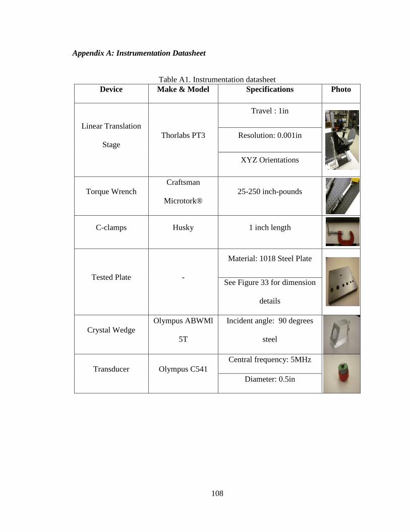
108

Appendix A: Instrumentation Datasheet

Table A1. Instrumentation datasheet Device Make & Model Specifications Photo

Linear Translation

Stage Thorlabs PT3

Travel : 1in

Resolution: 0.001in

XYZ Orientations

Torque Wrench Craftsman

Microtork® 25-250 inch-pounds

C-clamps Husky 1 inch length

Tested Plate -

Material: 1018 Steel Plate

See Figure 33 for dimension

details

Crystal Wedge Olympus ABWMl

5T

Incident angle: 90 degrees

steel

Transducer Olympus C541 Central frequency: 5MHz

Diameter: 0.5in

109

Appendix A(continued)

Table A1(continued).

Pulser/Recei

ver Olympus 5072PR

Amplificator range :

50dB

High Pass Filter: 1MHz

Low Pass Filter: 10MHz

Oscilloscope Tektronix TDS

2024B

Analog Bandwidth:

20MHz

Sample Rate: 2GS/s

Analog Channels: 4

110

Appendix B: Third Party Permissions

Figure B1. Publication permission NDT Resource Center.

A Novel Ultrasonic Method to Quantify Bolt Tension

Documents

Transcript of A Novel Ultrasonic Method to Quantify Bolt Tension