A Novel Technique to Determine the Controlling Unstable ...
8
© 2015 IJSRET 82 International Journal of Scientific Research & Engineering Trends Volume 1, Issue 5, Sept.-2015, ISSN (Online): 2395-566X A Novel Technique to Determine the Controlling Unstable Equilibrium Point in Power Systems Wagdy M. MANSOUR Email: [email protected] Mohamed A. ALI Email: [email protected] Nader SH. ABDELHAKEEM Email: [email protected] Faculty of Engineering (Shoubra), Benha University, Electrical Engineering Department, 108 Shoubra St., Cairo, Egypt. Abstract – The computation of the Unstable Equilibrium Point (UEP) is a key step involved in the direct methods of power system transient stability analysis. This paper presents an idea for formulating generalized energy function for the stability detection of interconnected power systems and obtained the UEP in an easy way. The energy function is formulated based on Energy functions for individual machines. The technique is validated by computing the Stable Equilibrium Point (SEP), the controlling UEP, and The Critical Clearing Time (CCT). Then, a Conventional Time Domain Method (CTDM) is used to validate the novel technique's results. Keywords – Online Transient stability, Real-time Transient Stability, Transient Energy Function (TEF), Stable Equilibrium Point (SEP), Unstable Equilibrium Point (UEP), Critical Clearing Time (CCT). I. INTRODUCTION In the past, transient stability has been evaluated using Transient Energy Function (TEF) [1-3], to calculate Critical Clearing Time (CCT). Transient Energy Function is known to be a very powerful tool of assessing CCT of a power system without solving the system dynamics equations at post fault. Alternatively, direct methods determine system stability based on energy functions. These methods adjudicate whether the system will remain stable or not once the fault is cleared, by comparing the system transient energy, at the end of a disturbance, to a critical energy value [4-7]. Assuming that the post fault system has a stable equilibrium, there is region of initial conditions in the state system space, from which the faulted system trajectories converge to a stable equilibrium. This is the stability region of the stable equilibrium point (SEP) [5]. When the power system is stressed, due to increase in volume and/or number of transactions or the occurrence of a major disturbance or both [8], [9], the system can lose stability. The computation of UEP is very important for stability region estimation. Among the transient energy function (TEF) methods, both the closest UEP method [11] and the controlling UEP method [10] need to compute the desired UEP. The closest UEP is the UEP having the lowest energy function value among all the UEPs on the stability boundary of the SEP. It is thus necessary to understand the characteristics of the equilibrium points and how these can affect the particular stability of the system. Several methods have been proposed to compute the closet UEP [11], [12]. This paper presents an efficient transient stability assessment using individual machines energy functions approach. A novel technique for computation of controlling unstable equilibrium points is proposed. The importance of the computation of the controlling UEP is further emphasized with a new methodology for improvement of stability margins based on the analysis of the controlling UEP. Thus, conditions for the separation of a machine (or a group of machines) are determined. Several test systems is employed to be simulated to prove the validity and effectiveness of the novel approach. II. THE POWER SYSTEM MODEL The power system is represented by the so-called classical model where generators are represented by constant voltage behind transient reactance and loads are modeled by constant impedance [13]. Furthermore, the motion of the generators is expressed with respect to the center of inertia (C.O.I.) of the system. For an n-generator system, let for generator i, E i , δ i Magnitude and angle of voltage behind transient reactance, respectively. ω i Rotor speed relative to asynchronous frame. M i Generator inertia constant. The position δo and speed ωo of the C.O.I. are defined by: 1 1 1 1 , n n o i i o i i i i t t M M M M (1) Where: 1 n t i i M M
Transcript of A Novel Technique to Determine the Controlling Unstable ...

© 2015 IJSRET
82
International Journal of Scientific Research & Engineering Trends
Volume 1, Issue 5, Sept.-2015, ISSN (Online): 2395-566X
A Novel Technique to Determine the Controlling
Unstable Equilibrium Point in Power Systems
Wagdy M. MANSOUR Email: [email protected]
Mohamed A. ALI Email: [email protected]
Nader SH. ABDELHAKEEM Email: [email protected]
Faculty of Engineering (Shoubra), Benha University, Electrical Engineering Department, 108 Shoubra St., Cairo, Egypt.
Abstract – The computation of the Unstable Equilibrium Point (UEP) is a key step involved in the direct methods of power
system transient stability analysis. This paper presents an idea for formulating generalized energy function for the stability
detection of interconnected power systems and obtained the UEP in an easy way. The energy function is formulated based on
Energy functions for individual machines. The technique is validated by computing the Stable Equilibrium Point (SEP), the
controlling UEP, and The Critical Clearing Time (CCT). Then, a Conventional Time Domain Method (CTDM) is used to
validate the novel technique's results.
Keywords – Online Transient stability, Real-time Transient Stability, Transient Energy Function (TEF), Stable Equilibrium
Point (SEP), Unstable Equilibrium Point (UEP), Critical Clearing Time (CCT).
I. INTRODUCTION
In the past, transient stability has been evaluated using
Transient Energy Function (TEF) [1-3], to calculate
Critical Clearing Time (CCT). Transient Energy Function
is known to be a very powerful tool of assessing CCT of a
power system without solving the system dynamics
equations at post fault. Alternatively, direct methods
determine system stability based on energy functions.
These methods adjudicate whether the system will remain
stable or not once the fault is cleared, by comparing the
system transient energy, at the end of a disturbance, to a
critical energy value [4-7]. Assuming that the post fault
system has a stable equilibrium, there is region of initial
conditions in the state system space, from which the
faulted system trajectories converge to a stable
equilibrium. This is the stability region of the stable
equilibrium point (SEP) [5]. When the power system is
stressed, due to increase in volume and/or number of
transactions or the occurrence of a major disturbance or
both [8], [9], the system can lose stability. The
computation of UEP is very important for stability region
estimation. Among the transient energy function (TEF)
methods, both the closest UEP method [11] and the
controlling UEP method [10] need to compute the desired
UEP. The closest UEP is the UEP having the lowest
energy function value among all the UEPs on the stability
boundary of the SEP. It is thus necessary to understand the
characteristics of the equilibrium points and how these can
affect the particular stability of the system. Several
methods have been proposed to compute the closet UEP
[11], [12].
This paper presents an efficient transient stability
assessment using individual machines energy functions
approach. A novel technique for computation of
controlling unstable equilibrium points is proposed. The
importance of the computation of the controlling UEP is
further emphasized with a new methodology for
improvement of stability margins based on the analysis of
the controlling UEP. Thus, conditions for the separation of
a machine (or a group of machines) are determined.
Several test systems is employed to be simulated to prove
the validity and effectiveness of the novel approach.
II. THE POWER SYSTEM MODEL
The power system is represented by the so-called
classical model where generators are represented by
constant voltage behind transient reactance and loads are
modeled by constant impedance [13]. Furthermore, the
motion of the generators is expressed with respect to the
center of inertia (C.O.I.) of the system.
For an n-generator system, let for generator i,
Ei, δi Magnitude and angle of voltage behind
transient reactance, respectively.
ωi Rotor speed relative to asynchronous frame.
Mi Generator inertia constant.
The position δo and speed ωo of the C.O.I. are defined
by:
1 1
1 1,
n n
o i i o i i
i it t
M MM M
(1)
Where: 1
n
t i
i
M M

© 2015 IJSRET
83
International Journal of Scientific Research & Engineering Trends
Volume 1, Issue 5, Sept.-2015, ISSN (Online): 2395-566X
The generator’s motion in the C.O.I. frame is defined as:
i i o
i i i o
(2)
Assume that the effect of damping is neglected in the
system; the generator’s equations of motion are given by
the following differential equations:
1,2, ,
i
i i i ei COI
t
i i
MM P P P
M
i n
(3)
The expressions for Pi, Pei and PCOI are given by:
2
i mi i iiP P E G
(4) 1
sin cosn
ei ij ij ij ij
jj i
P C D
n
ieiiCOI PPP
1
Where:
,ij i j ij ij i j ijC E E B D E E G
Pmi Mechanical power input.
Gii Real part of the ith diagonal element of
the network’s Y-matrix.
Cij, Bij Real and imaginary components of the
ijth element of the network’s Y-matrix,
respectively.
III. THE TRANSIENT ENERGY FUNCTION FOR
INDIVIDUAL MACHINE
Rearrange (3) for each machine at the post-fault
condition and multiplying it by θi˙, the following equation
can be obtained [14]:
0,
1,2, ,
i
i i i ei COI i
t
MM P P P
M
i n
(5)
Integrate (5) with respect to time, using to as lower limit,
where 0)( oi t and 0)( s
is
ioi t which is called
the Stable Equilibrium Point (SEP), yields
2
1
1
1( ) sin
2
cos
i
si
i i
s si i
ns
i i i i i i ij ij i
jj i
ni
ij ij i COI i
j tj i
V M P C d
MD d P d
M
(6)
Eqn. (6) is evaluated using the post fault network
configuration. The first term in Eqn. (6) represents the KE
of machine i with respect to the system COI. The
remaining terms are considered to be the PE. Thus, Eqn.
(6) can be expressed as:
i KEi PEiV V V (7)
Eqn. (7) consists of two parts: kinetic energy and
potential energy. Both energies need to be solved
numerically. After rotor angles are found numerically, the
energies can be represented by:
21
2i i iKE M (8)
1
1
cos( )( )
cos( )
sin( )
sin( )
i
si
sni js
i i i i ij
j i jj i
ni j
i
ij COI isj ti jj i
PE P C
MD P d
M
(9)
1
1 1
1 1
( )
cos( )
cos( )
sin( )
sin( )
i
si
ns
COI i i i
i
sn ni j
ij
i j i jj i
n ni j
ij si j i j
j i
P d P
C
D
(10)
The critical energy of machine i Vcritical_i is evaluated
where θi= θiu, wi=0 as indicated in eqn. (11).
_
1
1
( )
cos( )
cos( )
sin( )
sin( )
ui
si
u s
Critical i i i i
s un
i j
ij u uj i jj i
u un
i j
ij s uj i jj i
i
COI i
t
V P
C
D
MP d
M
(11)
1
1 1
1 1
( )
cos( )
cos( )
sin( )
sin( )
ui
si
nu s
COI i i i
i
s un n
i j
ij u ui j i j
j i
u un n
i j
ij s ui j i j
j i
P d P
C
D
(12)
Where: θu is the Unstable Equilibrium Point (UEP).
By the first integration of real power mismatch in eqn.
(3). The overall system energy function Vsystem [4] can be
written as:

© 2015 IJSRET
84
International Journal of Scientific Research & Engineering Trends
Volume 1, Issue 5, Sept.-2015, ISSN (Online): 2395-566X
2
2 1 1
1
1 1
1( )
2
(cos cos )
n n ns
system i i i i i i
i i i
n ns
ij ij ij ij
i j i
V V M P
C I
(13)
Where:
( ) ( )(sin sin )
s s
i j i j s
ij ij ij ijs
ij ij
I D
(14)
Thus, the sum of the individual machine energies is
equal to the total system energy and the critical energy for
overall system Vsys-critical is given by:
1
1
1 1
( )
(cos cos )
nu s
sys critical i i i
i
n nu s u
ij ij ij ij
i j i
V P
C I
(15)
Where:
( ) ( )(sin sin )
u u s s
i j i ju u s
ij ij ij iju s
ij ij
I D
(16)
IV. PROPOSED ALGORITHM
Correct determination of the SEP and UEP are essential
for the successful use of the transient energy function,
based on eqn. (3), the stable equilibrium point of the post
fault system is found by solving the following nonlinear
algebraic equations by the steepest descent method [15].
0, 1,2, ,i
i ei COI
t
MP P P i n
M (17)
The solution of such equations depends on the initial
values of δi, i = 1, 2, …, n, which can be chosen to be the
steady-state values of the prefault system.
If the fault is kept long enough for one or more machines
to become critically unstable, the potential energy of the
critical machine goes through a maximum before
instability occurs. Furthermore, this maximum value (of
the potential energy along the post disturbance trajectory)
of a given machine has been found to be a safe estimate of
the individual machine critical energy.
It was also shown in eqns. (8, 9, and 10) that a
reasonable choice for the critical value of Vi is VPei-max
along the system trajectory, and the value can be obtained
from the sustained fault conditions. By simulating a
sustained fault (or a fault of long duration), the potential
energy term of eqn. (9) are computed VPei, i = 1, 2, …, n
for each instant of time. The values of VPe-max are noted for
the different machines (or groups of machines). These
represent the value of Vcritical
_ max_Critical i PE iV V (18)
The value of VPe-max obtained represents the energy
absorbing capacity for each machine. It gives a measure of
the amount of kinetic energy converted to potential energy.
The unstable equilibrium point is found in the same way
as the stable equilibrium point by solving the following
nonlinear algebraic equations of (11, 18) by the steepest
descent method [15].
_
1
1
( )
cos( ) cos( )
sin( ) sin( )
0, 1,2, ,
ui
si
u s
Critical i i i i
ns u u u
ij i j i j
jj i
nu u s u
ij i j i j
jj i
i
COI i
t
V P
C
D
MP d i n
M
(19)
But the initial guess of δi, i = 1, 2, …, n, for the
minimization is chosen in such a way that the critical
machine can be chosen to be π-θs and the remaining
machines can be chosen to be θis.
To determine whether instability occurs, the total
transient energy at the instant of fault clearing is compared
with the value of VCritical for each machine. The mode of
instability is then given by those machines whose transient
energy at clearing exceeds their critical energy.
A Single Machine Infinite Bus (SMIB), this can be
derived as a special case of a multi-machine system as
follows. An infinite bus is equivalent to a machine having
infinite inertia and constant terminal voltage. If M2 → ∞,
the eqns. (7), (8), (9) and (11) respectively become:
_ _
2
max
_
max
1
2
( )
(cos cos )
( )
(cos cos )
SMIB KE SMIB PE SMIB
SMIB
s
SMIB m
s
postfault
u s
Critical SMIB m
u s
postfault
V V V
KE M
PE P
P
V P
P
(20)
V. SIMULATIONS AND RESULTS
Simulations have been conducted on both, single
machine infinite bus system and multi-machine system. In
this paper, the two machine infinite bus system shown in in
Fig.5 is used as the multi-machine system. The
conventional time domain solution and Transient Energy
Function (TEF) have been applied for transient stability
assessment. A three phase fault occurs on one of the
double lines in SMIB system and at bus 4 for multi-
machine system with line 4-5 cleared.
© 2015 IJSRET
85
International Journal of Scientific Research & Engineering Trends
Volume 1, Issue 5, Sept.-2015, ISSN (Online): 2395-566X
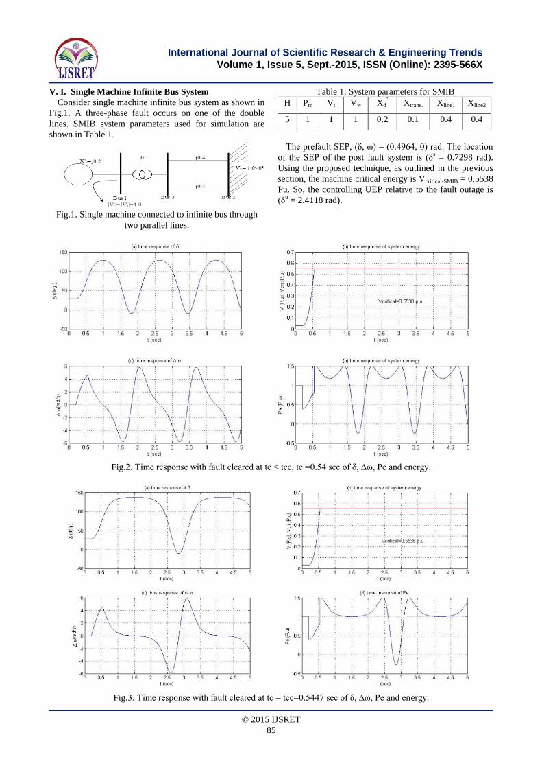
V. I. Single Machine Infinite Bus System
Consider single machine infinite bus system as shown in
Fig.1. A three-phase fault occurs on one of the double
lines. SMIB system parameters used for simulation are
shown in Table 1.
Fig.1. Single machine connected to infinite bus through
two parallel lines.
Table 1: System parameters for SMIB
H Pm Vt V∞ Xd’
Xtrans. Xline1 Xline2
5 1 1 1 0.2 0.1 0.4 0.4
The prefault SEP, (δ, ω) = (0.4964, 0) rad. The location
of the SEP of the post fault system is (δs = 0.7298 rad).
Using the proposed technique, as outlined in the previous
section, the machine critical energy is Vcritical-SMIB = 0.5538
Pu. So, the controlling UEP relative to the fault outage is
(δu = 2.4118 rad).
Fig.2. Time response with fault cleared at tc < tcc, tc =0.54 sec of δ, ∆ω, Pe and energy.
Fig.3. Time response with fault cleared at tc = tcc=0.5447 sec of δ, ∆ω, Pe and energy.

© 2015 IJSRET
86
International Journal of Scientific Research & Engineering Trends
Volume 1, Issue 5, Sept.-2015, ISSN (Online): 2395-566X
Fig.4. Time response with fault cleared at tc > tcc, tc=0.55 sec of δ, ∆ω, Pe energy.
Single machine swing curve and the energy under post-
fault condition are plotted at clearing times of 0.54 sec,
0.5447 sec and 0.55 sec as shown in Figs. 2, 3 and 4.
Fig.2 shows a stable case where the rotor angle oscillates
and reach another stable equilibrium point towards the end
of the transient and stability could be assured if the
transient energy at clearing condition δcl and ωcl remains in
the stable region or V(δcl , ωcl) < Vcr. The system is
critically stable with fault cleared at 0.5447 sec,
corresponding to a critical clearing angle δcr of 82.75
degrees and critical energy Vcr for the system investigated
is 0.5538, which is shown to be the maximum energy as
shown in Fig.3. When the fault is cleared at 0.55 sec,
system instability resulted and V(δcl , ωcl) > Vcr as
indicated in Fig.4.
The critical clearing time (tcc) can also be obtained from
the Pe versus time curve. That mean when Pe touch Pm in
the first swing, then tcc is obtained.
Fig.2 where tc<tcc, the Pe is higher than Pm in the first
swing. Fig.3 where tc=tcc, Pe touch Pm. When tc>tcc, the
system will be unstable as shown in Fig.4.
V.II. Multi-machine System The test system used contains two generators of finite
inertia and an infinite bus, as shown in Fig.5. The system
and prefault load flow data are given in Appendix; the
system has been simulated with a classical model for the
generators. The disturbance initiating the transient is a
three-phase fault occurring near bus 4 at the end of line 4–
5. The fault is cleared by opening line 4–5.
Fig.5. Network configuration of the test system.
The prefault SEP, (δ1, δ2, ω1, ω2) = (0.3634, 0.2826, 0,
0) rad. The location of the SEP of the post fault system is
(δ1s = 0.381058 rad, δ2
s = 0.277517 rad). Using the
proposed technique, the individual machines critical
energies are Vcritical-m/c1 =8.6872 Pu and Vcritical-m/c2 =0.0284
Pu. So, controlling UEPs relative to the fault outage are
(δ1u = 2.72937 rad1, δ2
u = 0.365294 rad).
Each machine swing curve, the phase trajectory in ∆ω-δ
plot and Energy functions for individual machines under
post-fault condition are plotted at clearing times of 0.4 sec,
0.405 sec and 0.41 sec as shown in Figs.6, 7 and 8. Fig.6
shows a stable case where the rotor angle oscillates, and
reach another stable equilibrium point towards the end of
the transient and stability could be assured if the transient
energy V1 (δcl, ωcl) < Vcritical1. The system is critically
stable with fault cleared at 0.405 sec, corresponding to a
critical clearing angle δcr1 of machine 1 (critical machine)
of 91.6588 degrees, critical energy Vcritical1 of machine 1
and the system investigated are 8.6872, 8.7156
respectively. When the fault is cleared at 0.41 sec, system
instability resulted and V1 (δcl, ωcl) > Vcritical1 as indicated
in Fig.8.

© 2015 IJSRET
87
International Journal of Scientific Research & Engineering Trends
Volume 1, Issue 5, Sept.-2015, ISSN (Online): 2395-566X
Fig.6. Time response with fault cleared at tc < tcc, tc =0.4 sec of δ, ∆ω, Pe, ∆ω versus δ and energy.
Fig.7. Time response with fault cleared at tc = tcc =0.405 sec of δ, ∆ω, Pe, ∆ω versus δ and energy.
Fig.8. Time response with fault cleared at tc > tcc, tc=0.41 sec of δ, ∆ω, Pe, ∆ω versus δ and energy.

© 2015 IJSRET
88
International Journal of Scientific Research & Engineering Trends
Volume 1, Issue 5, Sept.-2015, ISSN (Online): 2395-566X
The Critical Clearing Time (tcc) can also be obtained
from the Pe versus time curve. That mean when Pe of
critical machine touch Pm in the first swing, then tcc is
obtained.
Fig.6 where tc < tcc, the Pe is higher than Pm in the first
swing. Fig.7 where tc ≈ tcc, Pe touch Pm. When tc > tcc,
the system will be unstable as shown in Fig.8.
VI. CONCLUSION
In this paper complete model for transient stability
assessment of a multi-machine power system was
developed using MATLAB. The classical model of a
multi-machine power system using relative machine angle
reference formulation is employed and the individual
machine energy function is constructed. The stable
equilibriums are calculated from the solution of the power
flow equations, whereas the proposed method is used to
compute the unstable equilibrium point in easy way with
respect to other methods. Test results conducted on the
single and multi-machine power system. The results
obtained by this proposed approach are in good agreement
with those obtained by the time solution method.
APPENDIX
Line and transformer data*
From
Bus
To Bus Series Z Shunt Y
B R X
1 4 0.0 0.022 0.0
2 5 0.0 0.040 0.0
3 4 0.007 0.040 0.082
3 5 (1) 0.008 0.047 0.098
3 5 (2) 0.008 0.047 0.098
4 5 0.018 0.110 0.226
Generator data of test system*
Parameter G1 G2
Rated MVA 400 250
KV 20 18
Xd` 0.067 0.10
H 11.2 8.0
Prefault load flow data*
Bus Voltage Generation Load
P Q P Q
1 1.03∟8.88º 3.5 0.712 --- ---
2 1.02∟6.38º 1.85 0.298 --- ---
3 1.00∟0º --- --- --- ---
4 1.018∟4.68º --- --- 1.00 0.44
5 1.011∟2.27º --- --- 0.50 0.16
*All values are in per unit on 100MVA base.
REFERENCES
[1] P M. K. Khedkar, G. M. Dhole, V. G. Neve, “Transient
Stability Analysis by Transient Energy Function Method:
Closest and Controlling Unstable Equilibrium Point
Approach,” IE (I) Journal – EL, Vol. 85, pp. 83-88,
September 2004.
[2] W. Zhang, H. Zhang, and B.-S. Chen, “Generalized
Lyapunov equation approach to state-dependent
stochastic stabilization/detectability criterion”, IEEE
Trans. Autom. Control, Vol. 53, No. 7, pp. 1630–1642,
Aug. 2008.
[3] Samita Padhi, Bishnu Prasad Mishra: “Numerical Method
Based Single Machine Analysis for Transient Stability”
IJETAE, Vol. 4, February 2014.
[4] P. Varaiya, F. F. Wu, and R. L. Chen, “Direct methods
for transient stability Analysis of power systems: Recent
results,” Proc.IEEE, vol. 73, pp. 1703-1715, Dec 1985.
[5] L. Chen, Y. Min, F. Xu, and K. P. Wang, “A
continuation-based method to compute the relevant
unstable equilibrium points for power system transient
stability analysis,” IEEE Trans. Power Syst., vol. 24, pp.
165-172, Feb 2009.
[6] Wagdy M. Mansour, Mohamed A. Ali, Nader Sh. Abd-El
hakeem, "Combinational Protection Algorithm
Embedded With Smart Relays ", Journal of Electrical
Engineering: Vol. 15, Edition: 2, ISSN (Online): 1582-
4594, pp. 83-89. 2015.
[7] Wagdy M. Mansour, Mohamed A. Ali, Nader Sh. Abd-
El hakeem, " Online Modern Philosophy for Stability
Detection Based on Critical Energy of Individual
Machines", International Journal of Scientific Research
Engineering Technology Vol. 1, Issue 4, ISSN (Online):
2395-566X, Page(s): 50-57. July 2015.
[8] M. Shaaban, “A visual simulation environment for
teaching power system stability,” Int. J. of Electro. Eng.
Educ., vol. 47, pp. 357-374, Oct 2010.
[9] H. D. Chiang and J. S. Thorp, “The closest unstable
equilibrium point method for power system dynamic
security assessment,” IEEE Trans. Circuits Syst., vol. 36,
no. 9, pp. 1187–1199, Sep. 1989.
[10] T. Athay, R. Podmore, and S. Virmani, “A practical
method for direct analysis of transient stability,” IEEE
Trans. Power App. Syst., vol. PAS-98,pp.573–584, 1979.
[11] J. Lee, “Dynamic gradient approaches to compute the
closest unstable equilibrium point for stability region
estimate and their computational limitations,” IEEE
Trans. Autom.Control,vol.48,no.2,pp.321-324,Feb. 2003.
[12] J. Lee and H.-D. Chiang, “A singular fixed-point
homotopy method to locate the closest unstable
equilibrium point for transient stability region estimate,”
IEEE Trans. Circuits Syst. II, vol. 51, no. 4, pp. 185–189,
Apr. 2004.
[13] P. M. Anderson, A. A. Fouad, Power System Control and
Stability, John Wiley & Sons, Inc., 2003.
[14] Michel, A., Fouad, A., Vittal, V., “Power system
transient stability using individual machine energy
functions,” IEEE Transactions on Circuits and Systems,
vol.30, no.5, pp. 266- 276, May 1983.
[15] A. D. Booth, "An application of the method of steepest
descent to the solution of systems of non-linear
simultaneous equations," Quart. J. Mech. Appl. Math.,
vol. 2, pp. 460-463, December 1949.

© 2015 IJSRET
89
International Journal of Scientific Research & Engineering Trends
Volume 1, Issue 5, Sept.-2015, ISSN (Online): 2395-566X
AUTHOR PROFILE
Prof. Dr.-Eng. Wagdy M. Mansour He received the B.Sc. degree in electrical
engineering from Mansoura University in 1967.
In 1974 he received his M.Sc. from Helwan
University and in 1980 a Ph.D. in control
engineering from the Technical University of
Braunshweig –Germany. Since 1990 he has
been a professor of control of power systems at the faculty of
engineering, Benha University, Cairo (Egypt). (Benha
University, Faculty of Engineering, Elec. Eng. Dep., 108
Shoubra Street, Cairo/Egypt).
Dr.-Eng. Mohamed A. Ali He received the B.Sc., M.Sc., and PhD degree
in electrical engineering from Zagazig
University, Benha University, Egypt,
respectively. His practical experience included
the power system protection systems up to the
500kV level with the application on the Egyptian electrical grid.
His research interests are power system analysis, stability,
control and protection
Assist. Lecturer-Eng. Nader Sh.
Abd El-Hakeem He received the B.Sc. degree in electrical
engineering from Benha University in 2006
and in 2012 he received his M.Sc. from Benha
University. Since 2009 he has been an
Administrator at the faculty of engineering, Benha University,
Cairo (Egypt).