Mechanical Engineering - Daytona Beach College of Engineering

2013

A Novel Method for Prediction of Mobile Robot Maneuvering A Novel Method for Prediction of Mobile Robot Maneuvering

Spaces Spaces

Patrick N. Currier Embry-Riddle Aeronautical University, currierp@erau.edu

Alfred L. Wicks Virginia Polytechnic Institute and State University

Follow this and additional works at: https://commons.erau.edu/db-mechanical-engineering

Part of the Mechanical Engineering Commons

Scholarly Commons Citation Scholarly Commons Citation Currier, P. N., & Wicks, A. L. (2013). A Novel Method for Prediction of Mobile Robot Maneuvering Spaces. Journal of Terramechanics, 50(2). Retrieved from https://commons.erau.edu/db-mechanical-engineering/2

https://doi.org/10.1016/j.jterra.2013.03.001 This Article is brought to you for free and open access by the College of Engineering at Scholarly Commons. It has been accepted for inclusion in Mechanical Engineering - Daytona Beach by an authorized administrator of Scholarly Commons. For more information, please contact commons@erau.edu.

A NOVEL METHOD FOR PREDICTION OF MOBILE ROBOT

MANEUVERING SPACES

Patrick N. Curriera1*

and Alfred L. Wicksb

aVirginia Polytechnic Institute and State University – Dept. of Mechanical Engineering – 114

Randolph Hall, Blacksburg, VA USA 24061

bVirginia Polytechnic Institute and State University – Dept. of Mechanical Engineering – 114

Randolph Hall, Blacksburg, VA USA 24061 – awicks@vt.edu

Abstract

As the operational uses of mobile robots continue to expand, it becomes useful to be able to

predict the admissible maneuvering space to prevent the robot from executing unsafe maneuvers.

A novel method is proposed to address this need by using force-moment diagrams to characterize

the robot’s maneuvering space in terms of path curvature and curvature rate. Using the proposed

superposition techniques, these diagrams can then be transformed in real-time to provide a

representation of the permissible maneuvering space while allowing for changes in the robot’s

loading and terrain conditions. Simulation results indicate that the technique can be applied to

determine the appropriate maneuvering space for a given set of loading conditions, longitudinal

acceleration, and tire-ground coefficient of friction. This may lead to potential expansion in the

ability to integrate predictive vehicle dynamics into autonomous controllers for mobile robots

and a corresponding potential to safely increase operating speeds.

Keywords: mobile robots, maneuvering spaces, predictive dynamics

1 Embry-Riddle Aeronautical University – Dept. of Mechanical Engineering – 600 S. Clyde

Morris Blvd, Daytona Beach, FL USA 32114 –Email: currierp@erau.edu

* Corresponding Author

1 Introduction

This work proposes a methodology for real-time prediction of the dynamic operating

envelope of a large mobile robot. The method abstracts a vehicle model of arbitrary complexity

using a force-moment representation that can then be transformed into an operating manifold

expressed in terms of motion variables to outline vehicle performance limitations. Additionally,

the method allows for realistic variation in vehicle Center of Gravity (CG), longitudinal

acceleration, and terrain surface conditions as represented by a coefficient of friction.

1.1 Background

Large scale robotic demonstrations such as the DARPA Grand Challenges have

demonstrated the potential inherent in applying autonomous technologies to large mobile robots

operating at high speed over uncertain terrain. In these conditions, the dynamics of the vehicle

can become highly significant to the ability of the robot to safely maneuver and failures modes,

such as roll-over, that can be largely overlooked in smaller rovers can have catastrophic

consequences. To avoid this type of failure, shown in Fig 1, it is necessary for an autonomous

controller to have the ability to predict and compensate for the dynamic limits of the vehicle [1].

Fig. 1: Rollover of large mobile robot due to an attempted maneuver beyond the vehicle’s dynamic limits.

Despite evidence of this need, many current autonomous controllers rely on simple kinematic

models to define vehicle limitations in the planning and execution stages of control [2]. The

kinematic, bicycle model is widely used due to ease of implementation and, when implemented

with an appropriate understeer coefficient, reasonable accuracy in predicting motion of the class

of Ackerman-steered vehicles that are commonly used for large mobile robotics [3]. The bicycle

model compresses the two wheels on each axle of a vehicle into a single track, and is thus unable

to account for the non-linear effects of lateral normal force transfer that can significantly affect

the handling dynamics of a vehicle [4][5]. These kinematic models are generally adequate for

defining the non-holonomic motion constraints, but may allow for trajectories that are non-

admissible due to dynamic constraints to be considered and executed [6].

Additionally, most high-level planning work to date relies on the assumption that the vehicle

and terrain conditions are invariant, particularly in regards to vehicle load the tire-ground

coefficient of friction [7]. Several techniques have been developed to estimate these important

quantities based on measurements of vehicle state. These techniques, however, stop short of

integrating these estimates into mobile robot planning [8][9][10][11][12].

2 Methods

One of the primary potential advantages of autonomous controllers on mobile robots is the

ability to use feed-forward controllers to avoid potentially dangerous situations instead of

attempting to compensate with feedback. In order to allow this use, it is necessary to create a

function that can map the feed-forward control inputs to the predicted dynamic state output. For

the class of four-wheeled, Ackerman-steered mobile robots considered in this work, the control

inputs are the steering angle of the front wheels and the torque at the wheels as dictated by the

drive and/or brake settings. The outputs are the motion variables; these will be defined as a path

curvature, curvature rate, longitudinal velocity, and longitudinal acceleration.

An accurate dynamic vehicle model must consider a very large number of effects; a

multibody commercial dynamic model such as VehicleSim may include more than 200 degrees-

of-freedom [13]. Due to the complexity of the factors involved when dynamic effects are

considered, it becomes difficult to derive a tractable closed-form solution to the desired feed-

forward function. Additionally, many autonomous controllers rely on search techniques to

determine an optimal path from a candidate space. These techniques require the feed-forward

function to be supply an entire space of admissible trajectories in real-time and not just a single

solution.

The proposed method uses a numerical solver to precalculate the motion variable outputs

from a vehicle model across the entire potential maneuvering space. These results can be stored

and then accessed in real-time by the feed-forward controller by applying superposition

techniques based on the current state of the vehicle.

2. 1 Modeling Technique

To simplify the vehicle model into a form that can be stored, a quasi-static force-moment

representation is used. This method, championed by Milliken represents the maneuvering state of

the vehicle in terms of lateral and longitudinal forces and yawing moments, as illustrated in Fig.

2 [14]. The searchable operating space can be characterized in coordinates of the lateral slip

angles at the front and rear wheels. The force-moment diagram can be solved numerically across

the searchable space for the lateral force, longitudinal force, and yawing moment.

This representation has the effect of abstracting the specifics of the actual vehicle model from

the remainder of the method. A vehicle model of arbitrary complexity can be used, provided that

it can be solved for the appropriate coordinates and variables. Using numerical solution

techniques, it is therefore possible to build a quasi

taking the highly non-linear aspects of components such as tires in

Fig. 2: Example of a manuever space in terms of path curvature versus curvature rate at a

space of front and rear slip angles.Each line with a negative slope represents a constant front wheel steering angle and each line

with a positive slope indicates a constant body slip angle.

For purposes of this work, a relativel

system) model incorporating lateral

linear Fiala tire model was implemented in MATLAB.

wheel representation formulated by Will and Zak and was selected as the simplest representation

capable of capturing the critical sprung mass weight transfer response to accelerations

model has a total of 11 degrees of freedom: translation in the

rotation of the vehicle about the z

rotation of the sprung mass about the

individual wheel ( ), and location of the sprung mass center of gravity

fixed vehicle axes ( ).

be variable within bounds due to the effects of payloads (such a

The vehicle frames are shown in Fig

Fig. 3: Vehicle coordinate frames showing location of vehicle frame at the center of the rear axle and its relationship to the CG

and wheel frames.

possible to build a quasi-static map of the vehicle performance while

linear aspects of components such as tires in to account.

a manuever space in terms of path curvature versus curvature rate at a constant longitudinal force across the

Each line with a negative slope represents a constant front wheel steering angle and each line

with a positive slope indicates a constant body slip angle.

For purposes of this work, a relatively simple (when compared to a multi-body commercial

model incorporating lateral and longitudinal load transfer and a combined

linear Fiala tire model was implemented in MATLAB. The model is based on the simplified 4

rmulated by Will and Zak and was selected as the simplest representation

capable of capturing the critical sprung mass weight transfer response to accelerations

model has a total of 11 degrees of freedom: translation in the x, y, and z body-fixed vehicle axes,

z-axis ( ), rotation of the sprung mass about the

rotation of the sprung mass about the y-axis ( ), steering of the front wheels ( ), rotation of each

location of the sprung mass center of gravity relative to the body

). The model is assumed to have a known CG location that may

be variable within bounds due to the effects of payloads (such as cargo) carried by

The vehicle frames are shown in Fig. 3.

Vehicle coordinate frames showing location of vehicle frame at the center of the rear axle and its relationship to the CG

static map of the vehicle performance while

itudinal force across the

Each line with a negative slope represents a constant front wheel steering angle and each line

body commercial

combined-slip, non-

The model is based on the simplified 4-

rmulated by Will and Zak and was selected as the simplest representation

capable of capturing the critical sprung mass weight transfer response to accelerations [15]. The

fixed vehicle axes,

, rotation of the sprung mass about the x-axis ( ),

), rotation of each

relative to the body-

The model is assumed to have a known CG location that may

s cargo) carried by the vehicle.

Vehicle coordinate frames showing location of vehicle frame at the center of the rear axle and its relationship to the CG

During maneuvering of a standard vehicle, assumed for purposes of this work to be a 4-

wheeled vehicle with suspended wheels and front-wheel steering, significant weight transfers can

and will occur in response to lateral (y-axis) and longitudinal (x-axis) accelerations. These weight

transfers can be modeled as acting through the roll centers of the suspension, which are defined

as the point at which a lateral force applied to the sprung mass does not create a rolling moment

[14]. The roll centers are determined kinematically and can move in response to suspension

jounce, but this movement is assumed to be small and neglected for this model. Suspension

effects can be generalized and separated into orthogonal components by modeling the connection

between the sprung and unsprung masses as a revolute joint placed at each roll center oriented

along the roll axis and an additional joint oriented parallel to the vehicle y-axis at the pitch

center.

Assuming that the vehicle is operating on a roughly planar surface, the longitudinal portion

of the weight transfer (∆���) at axle N will occur primarily due to throttle and brake inputs and

can be modeled by taking moments about the contact patches [14]:

∆��� � � �ℓ �� � �������� (1)

∆��� � �ℓ �� � �������� (2)

where g is the acceleration due to gravity, �� is the effective rolling radius of the wheels, �� is

the mass of the sprung body, �� is the longitudinal acceleration due to throttle or brake input,

and ℓ is the effective wheelbase.

Lateral weight transfer occurs primarily due to the lateral accelerations acting on the CG during

turning maneuvers. The roll axis defined by the roll centers causes this to be governed by a

characteristic height (H) that is the Euclidean distance between the CG and the roll axis at the

longitudinal location of the CG:

� � �� � �� � �ℓ ������� � ����ℓ � �� �� (3)

where ���� represents the height of the roll center of axle N relative to the vehicle frame. This

height can then be used to derive the effect of lateral acceleration (∆���) by taking moments

about one side of the vehicle, as shown by Milliken [14]:

∆��� � ���� !"#$%�����&���'� !"#�()'� !$� � ����� *���(�ℓ%� (4)

where +,�is the effective roll stiffness of axle N, -. represents the track width of the axle N, and Λ0 � �� or Λ� � ℓ � �� . Additional weight transfer from the nominal values may occur due

to lateral CG offsets. This can be calculated using a normalized coefficient for each wheel n

(1�2) [14]:

1�2 � �3 � 45�67� � �()8.:%�. (5)

The total instantaneous weight distribution (;<2� can then be found by calculating the static

weight distribution (;�2� and superimposing the dynamic effects:

;�2 � �ℓ 1�2���Λ. � �=� (6)

;<2 � ;�2 � ∆��� � 1�2∆��� (7)

to yield the total expected normal force on each wheel.

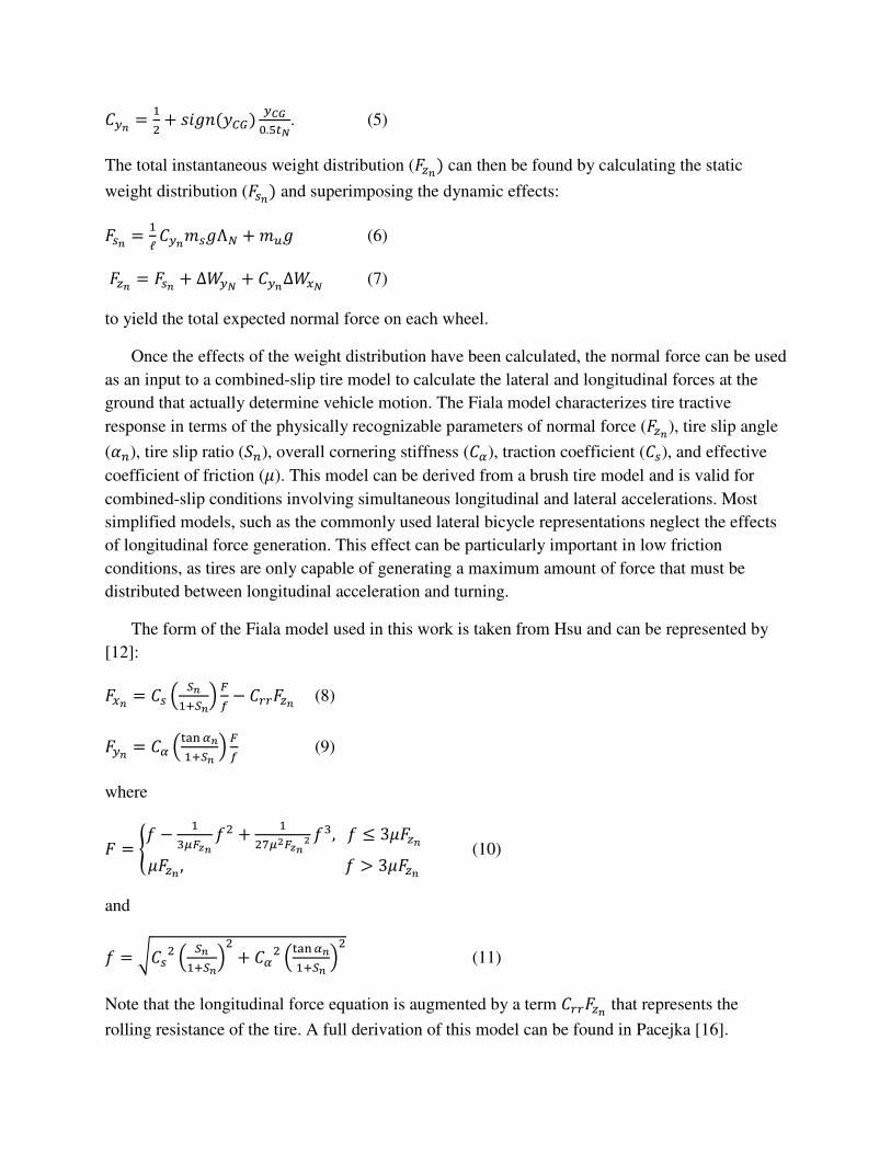
Once the effects of the weight distribution have been calculated, the normal force can be used

as an input to a combined-slip tire model to calculate the lateral and longitudinal forces at the

ground that actually determine vehicle motion. The Fiala model characterizes tire tractive

response in terms of the physically recognizable parameters of normal force (;<2), tire slip angle

(>?), tire slip ratio (@?), overall cornering stiffness (1A), traction coefficient (1�), and effective

coefficient of friction (B). This model can be derived from a brush tire model and is valid for

combined-slip conditions involving simultaneous longitudinal and lateral accelerations. Most

simplified models, such as the commonly used lateral bicycle representations neglect the effects

of longitudinal force generation. This effect can be particularly important in low friction

conditions, as tires are only capable of generating a maximum amount of force that must be

distributed between longitudinal acceleration and turning.

The form of the Fiala model used in this work is taken from Hsu and can be represented by

[12]:

;�2 � 1� � C2�&C2� 0D � 1EE;<2 (8)

;�2 � 1A �FGH A2�&C2 � 0D (9)

where

; � IJ � �KL0M2 J3 � �

3NLO0M2O JK, J R 3B;<2B;<2 , J T 3B;<2U (10)

and

J � V1�3 � C2�&C2�3 � 1A3 �FGH A2�&C2 �3 (11)

Note that the longitudinal force equation is augmented by a term 1EE;<2 that represents the

rolling resistance of the tire. A full derivation of this model can be found in Pacejka [16].

From the tire model, the contribution of each wheel to the total lateral (;�) and longitudinal

(;�) forces acting on the vehicle can be determined. These forces can thus be summed in the

vehicle frame after correcting for the steering angle (W.):

;� � ∑ ;�2 cos W. � ;�2 sin W.?̂_8 (12)

;� � ∑ ;�2 sin W. � ;�2 cos W.?̂_8 (13)

The overall yawing moment (M) about the vehicle frame can be determined by summing the

cross products of the resultant vector wheel forces (;?�:

` � ∑ a? b ;??̂_� (14)

where a? is the position vector from the vehicle frame origin to the center of wheel n.

This non-linear model was numerically solved in terms of the coordinates of steering angle W) and body slip angle (c) using a trust-region-dogleg algorithm implement in the MATLAB

function fsolve to find the resultant lateral force and yawing moment over the grid of angular

coordinates for a fixed longitudinal force to create a set of force-moment diagrams. The values in

the diagrams were then non-dimensionalized using the weight and wheelbase of the vehicle as

the normalizing terms to form a lateral force coefficient 1d and a yawing moment coefficient 1e.

For purposes of navigation and control, a representation of vehicle performance in terms of

motion variables is desirable, necessitating a transformation from force-moment coordinates to

path curvature, curvature rate, and acceleration. Since the knowledge of the state of these

variables allows for prediction of the future path of the vehicle, this defines a “maneuver space”

consisting of the set of achievable path variables. A vehicle operating at a point within this space

with a zero curvature rate will trace a path of a circle with a radius equal to the inverse of the

path curvature while a vehicle with a non-zero curvature rate will trace a path of increasing or

decreasing radius. The edges of the space indicate the limits of vehicle performance, i.e. the

largest path curvature contained within the space represents the minimum achievable turning

radius, even if this minimum radius may not be sustainable at steady state (as indicated by a non-

zero curvature rate).

Assuming a current or desired longitudinal velocity is known, the path curvature can be

calculated by assuming that all of the lateral force is used to offset the centripetal force due to

curvilinear motion [14]:

f � �g!hiO (15)

where f is the instantaneous vehicle path curvature or the inverse of the turning radius and j� is

the longitudinal speed in the direction of the vehicle frame x-axis.

An expression can then be derived to relate the yawing moment to a rate of change of curvature:

ekM � ��lℓ

kM � mn � oo% j�f� (16)

��lℓkM � j�p f � j�fp (17)

fp � ���lℓkM � j�p f� �

hi (18)

where fp is the instantaneous rate of change of curvature and q< is the moment of inertia about the

z-axis. In many cases the exact moment of inertia is unknown but can be approximated using the

dynamic index [17]:

rq � EMO�()ℓ'�()� (19)

where s< is the radius of gyration of the vehicle. For most vehicles, the dynamic index is

approximately equal to unity, with slightly lower values found on high performance vehicles

[17]. The moment of inertia is related to the dynamic index by:

q< � ���� ℓ � �� �rq (20)

and can thus be reasonably approximated for most vehicles using knowledge of the mass of the

sprung body and the location of the CG.

Once the curvature coordinates have been transformed, it becomes useful to transform the

slip angles into the more useful coordinates of the front wheel steering angle and body slip angle.

Kinematics can be used to derive an expression for the steering angle [14]:

W � t-t6ℓf� � >E � >D (21)

Since the commonly used navigation frame is located at the center of the rear axle,

transformation of the rear slip angle to the body slip angle is trivial in a front-steer only vehicle.

Provided that the solution grid is dense enough, these angular transformations can be performed

by linear interpolation.

2.2 Parameter Variation

An important aspect of this work is the ability to account for temporal variations in both

vehicle load and terrain conditions. In order to do this, it is necessary to have an estimate of the

current values of these parameters. Estimation of these values is beyond the scope of this work,

but techniques are further developed in [18].

Assuming that the load state of the vehicle can be estimated, it becomes necessary to define a

method for incorporating that knowledge into estimates of the maneuvering space. To do this, the

load state of the vehicle can be defined in terms of the mass of the vehicle and the location of the

CG relative to the navigation frame in three dimensions. This definition assumes that the CG

location of a typical vehicle in its empty state can be known and that changes in CG are likely to

be affected mainly by the addition of cargo or passengers. Furthermore, it is assumed that the

parameters of the load state can be reasonably bounded based on known vehicle characteristics.

An example of this would be a pickup truck with a rear bed. The location of the CG of the

pickup truck when carrying no bed load, fuel, or passengers can generally be known. This state is

considered the “empty” load state of the vehicle. As passengers and cargo are added, the total

vehicle CG location will change in response to the added mass. On a vehicle such as a pickup

truck, it is reasonable to place bounds on the mass based on the rated capacity of the truck and on

the CG location by making assumptions as to likely locations of this mass (i.e. the x location of

the CG is likely to shift farther in the direction of the cargo bed than in the direction of the cab).

Although techniques for doing so are beyond the scope of this paper, it is possible in many cases

to measure, estimate, or input parameters to allow for calculation of the current load state based

on the current cargo configuration.

Using the techniques developed in the previous section, it is possible to precalculate the

maneuvering space of the vehicle for any arbitrary location of the CG. Conveniently the mass

can be factored out of the equations and is not necessary if the CG location is known. The

obvious difficulty with this technique is that it is usually infeasible to precalculate maneuvering

space maps for all possible (or even all likely) CG locations as the number of combinations

becomes intractable for even coarse discretizations due to the potential variation in three

dimensions.

This difficulty can be addressed by the simple realization that the maneuvering

characteristics of the vehicle are determined by the forces and moments acting on the body; these

forces and moments have already been approximated by the numerical solution technique. It is

therefore possible to decouple the three dimensional variation and precalculate the effect of

movement of the CG in any one dimension on the resultant forces. These effects can be

calculated over a relatively small number of cases represented by a discretization of likely CG

locations.

Using the pickup truck example, the resultant forces would first be calculated for the empty

truck using the known CG location. By applying domain knowledge, a set of likely �� locations

can be formulated and the resultant forces that would occur in this load state can be calculated.

For the pickup truck, this set would likely include a small number of values of CG location

forward of the empty CG (assuming only passengers) and a larger number of values to the rear of

the empty CG location (assuming heavy cargo). This procedure can be repeated for the

decoupled 7� and �� parameters. If a set of size 10 is used for each variable, this would require

calculation of 30 loaded cases plus the empty case. If these sets are not decoupled, this would

require calculation of approximately 1000 independent load cases, which would be much more

expensive in terms of computation and storage of results.

The results of the computation of the decoupled load cases are a set of predicted lateral forces

and yawing moments expressed in terms of the non-dimensionalized coefficients 1d and 1e.

Although the couplings between load states with different 3D CG locations are non-linear, when

the resultant effects are expressed in terms of forces and moments, it becomes possible to

linearly interpolate the results of the decoupled solutions and achieve a reasonable estimate of

the uncalculated coupled solution:

u � u��v%� � wu�xyz{|{'u��v%�} � wu�xyz{|{'u��v%�} � wu<xyz{|{'u��v%�} (22)

` � �̀�v%� � w`�xyz{|{' �̀�v%�} � w`�xyz{|{' �̀�v%�} � w <̀xyz{|{' �̀�v%�} (23)

where the subscript empty indicates the force or moment result produced by the unloaded vehicle

case and the subscript loaded indicates the result produced by the decoupled CG offset case. For

example, if the location of the loaded CG were determined to be simultaneously offset from the

empty CG by 0.1m in the x direction, 0.05m in the y direction, and 0.2m in the z direction, the

loaded terms would consist of the results from the precalculated cases of a 0.1m x offset

(assuming empty case y and z locations), of a 0.1m y offset (assuming empty case x and z

locations), and of a 0.1m z offset (assuming empty case x and y locations). The output of Eqs. 22-

23 would represent the estimate of forces produced by the 3D dimensional offset without the

need to directly calculated the coupled result. It can also be seen by inspection that Eqs. 22-23

can be reduced to:

u � �2u��v%� � u�xyz{|{ � u�xyz{|{ � u<xyz{|{ (24) ` � �2 �̀�v%� � `�xyz{|{ � `�xyz{|{ � <̀xyz{|{ (25)

The resultant superimposed forces and moments can then be transformed using Eqs. 15-18 to

yield an estimate of the maneuvering space for the vehicle in the load condition represented by

the offset CG. If a higher fidelity for load cases between the discretizations is desired, it is also

possible to linearly interpolate for any value of CG coordinates between the precomputed

discretizations.

2.2 Friction and Acceleration Effects

Another important characteristic that determines vehicle performance capabilities is the

ability of the tire to produce force due to its contact with the terrain surface. Without delving into

the intricacies of terramechanics, variations in the terrain conditions can be largely characterized

in terms of the tire ground coefficient of friction. Changes in the friction coefficient can have an

enormous impact on the available maneuvering space for a mobile robot. Any driver who has

ventured onto black ice on a highway and lost control of his or her vehicle can likely verify this

claim. This effect results from the reduction of the total amount of force generation capability

available to the tire, a number that can be grossly represented as the product of the coefficient of

friction and the normal force. As the coefficient of friction decreases, the tires can no longer

produce enough force to hold the vehicle on the desired trajectory against the effects of inertial

and centripetal forces.

As can be noted from the references cited previously, estimation of the friction coefficient in

real-time and in realistic driving conditions is a decidedly non-trivial undertaking. Accuracy

tends to be low and precision is largely determined by the level of excitation in the system. As a

result, it is logical to partition the friction space into a small, discrete number of bins, as shown

in Table 1, for purposes of integration into a maneuvering space mapping algorithm.

Table 1: Friction space partitions

Coefficient

Range

Likely Terrain

Surface

0.75-1.0 Dry paved road

0.50-0.75 Wet paved road or

hard unpaved road

0.25-0.50 Soft unpaved road or

snow

0.0-0.25 Wet mud or ice

As changes in the friction coefficient with this coarse discretization tend to have far more

significant effects on the resulting force-moment diagram than changes in CG location, it

becomes difficult to achieve good results by applying the type of superposition used for CG

variation. However, it is possible to exploit the coarse binning of the friction coefficient by

simply calculating the resultant forces for each friction bin. This approach would be

computationally intractable without the proposed superposition algorithm as even the limited

partition of the friction space requires a four-fold increase in computation time. The reduced

number of computational cases, �� versus �K, required by the decoupling of CG variables

enables this the be a feasible approach.

An often neglected aspect of vehicle performance in navigation algorithms is the effect of

longitudinal acceleration on the maneuver space. The total amount of force available from the

tires is limited by the normal forces and coefficient of friction. Any force required to

longitudinally accelerate the vehicle is thus not available to produce a lateral path change. This

effect is often referred to as the friction ellipse [14]. Intuitively, this makes sense as a vehicle

under heavy braking will tend to slide when a turn that could normally be executed is attempted.

This problem is particularly relevant to autonomous systems as rapid turn maneuvers are

typically only needed in emergency situations such as obstacle avoidance when the vehicle is

also likely to be braking.

Similarly to the coefficient of friction, this effect can be handled by partitioning the

acceleration cases into a limited set of acceleration values. The exact values used would depend

on the capabilities of the vehicle but a set such as: steady-state road load, hard braking, moderate

braking, hard throttle is suggested. This further increases the computational complexity of the

precalculations. To account for both friction and acceleration effects the number of precalculated

cases required becomes:

# �t4�4 � # B �t4�4�# �� �t4�4�# �� �t4�4 � # 7� �t4�4 � # �� �t4�4� (26)

When bounded by reasonable domain knowledge, the size of the result of Eq. 26 can be

controlled will almost always be much smaller than the required number of cases for calculation

all possible permutations of friction, acceleration, and CG location.

3. Results

To show the effect of the developed methodology, a model of a small rear-wheel drive truck

was implemented in MATLAB and tested against a multi-body representation of the same

vehicle using Mechanical Simulation’s TruckSIM package.

To test the accuracy of the force-moment modeling technique, the TruckSIM model was

driven with the integrated driver model over a 3km road course to generate a set of control

inputs. These control inputs were then fed into an open-loop Simulink simulation using the

force-moment model and the resultant trajectories are shown in Fig. 4. As can be seen in Table 2,

the Simulink simulation, despite running in pure open-loop mode produced mean relative path

errors (path error per total distance traveled) of 5% or less.

Table 2: Force-moment simulation results

Name Velocity µ % Error

Case 1 30 kph 1.0 3.8%

Case 2 Varying 20-50 kph 1.0 5.0%

Case 3 50% of Case 2 1.0 4.4%

Case 4 50% Throttle 1.0 1.7%

Case 5 30 kph 0.5 3.5%

Fig. 4: Results of simulation using force-moment model with CG variation as given by Table 2. Note that although the

simulation was run purely open loop, the desired trajectory is acccurately recreated.

To demonstrate the need for an adaptive model in terms of load condition, a similar set of

runs was executed using CG heights and masses that were intentionally set to values different

from that of the TruckSIM model

CG height and vehicle mass of the force

differing simulation tracks. These results indicate that more advanced knowledge of the actual

load state of the vehicle would be beneficial to increase accuracy of the model predictions,

although the effect is small in this case.

by the relative insensitivity of the vehicle to changes in CG heigh

testing involving variation of additional parameters and testing involving a live vehicle with

varying CG appears to be warranted in order to confirm these results.

Table 3: CG variation parameters

Name CG

Height

Case 1

(nominal)

0.50m

Case 2 0.75m

Case 3 0.50m

Case 4 0.75m

Case 5 0.50m

Case 6 0.75m

Fig. 5: Results of simulation using force-moment

tracks compared to the results of Fig. 4 as parameters are varied from nominal.

3.1 CG Location Variation

The effect of variations in decoupled CG position as loading conditions

demonstrated by calculating the maneuvering manifold for a set of varying parameters

from a positive 0.1m offset to a negative 0.5m offset

produces a significant change in the maneuvering spa

To demonstrate the need for an adaptive model in terms of load condition, a similar set of

runs was executed using CG heights and masses that were intentionally set to values different

from that of the TruckSIM model, as shown in Table 3. As can be seen in Fig. 3, variation

of the force-moment model from the nominal configuration

These results indicate that more advanced knowledge of the actual

d state of the vehicle would be beneficial to increase accuracy of the model predictions,

although the effect is small in this case. The small magnitude of the effect is likely exacerbated

by the relative insensitivity of the vehicle to changes in CG height, as shown in Fig.

testing involving variation of additional parameters and testing involving a live vehicle with

varying CG appears to be warranted in order to confirm these results.

arameters results

Mass Relative Path Error

1000kg 5.3%

1000kg 5.2%

1500kg 7.4%

1500kg 5.1%

2000kg 7.5%

2000kg 7.2%

moment model with CG variation as given by Table 3. Note the divergence in the path

as parameters are varied from nominal.

Variation & Superposition

The effect of variations in decoupled CG position as loading conditions change can be

demonstrated by calculating the maneuvering manifold for a set of varying parameters

from a positive 0.1m offset to a negative 0.5m offset. As shown in Fig. 6, variation of

produces a significant change in the maneuvering space. The available curvature rate increases

To demonstrate the need for an adaptive model in terms of load condition, a similar set of

runs was executed using CG heights and masses that were intentionally set to values different

3, variations of the

moment model from the nominal configuration produce

These results indicate that more advanced knowledge of the actual

d state of the vehicle would be beneficial to increase accuracy of the model predictions,

The small magnitude of the effect is likely exacerbated

t, as shown in Fig. 8. Further

testing involving variation of additional parameters and testing involving a live vehicle with

e divergence in the path

change can be

demonstrated by calculating the maneuvering manifold for a set of varying parameters ranging

, variation of

ce. The available curvature rate increases

size but the vehicle becomes less stable as indicated by the peaks of the plot crossing into the

negative curvature half-plane. This can be classified as an oversteer condition and would be

expected as the CG is shifted aft in the vehicle. A forward shift in CG results in a decrease in

curvature rate and an increase in more stable understeer behavior.

Fig. 6: Plot of manuevering space diagrams showing the effect of variaiton of the x position of the CG. Note that the vehicle

tends to oversteer (the peaks of the plot cross the curvature axis) as the CG shifts rearward.

The vehicle was also simulated over a range of values for CG variation in the y and z

directions. The CG was shifted by a magnitude of 0.3m in each direction on the y-axis and over a

range from negative 0.1m to 0.4m in the z-axis. As can be seen in Fig. 7-8, the vehicle showed a

small sensitivity to shifts in both axes. The diagram shows slight deformation near the handling

boundaries, but the overall effect is minimal. This result is not entirely unexpected, as the CG

location in these axes does not tend to have a large impact on the understeer/oversteer

characteristics of a vehicle [14].

A much larger impact due to variations in these axes is seen in terms of the rollover

tendencies. Although not discussed in this paper, this technique can be extended to calculation of

dynamic stability indices. These indices show large and significant changes as a result of CG

variation in the y and z axes. Further discussion of this phenomenon can be found in [18].

Fig. 7: Plot of manuevering space diagrams showing the effect of variaiton of the y position of the CG. Note that the vehicle is

largely insensitive to variation in this parameter in terms of manuevering space, although some effect is seen near the upper and

lower bounds of the plot.

Fig. 8: Plot of manuevering space diagrams showing the effect of variaiton of the z position of the CG. Note that the vehicle is

largely insensitive to variation in this parameter in terms of manuevering space.

The efficacy of the superposition technique for estimation of the resultant maneuvering space

for variation in CG was tested by directly calculating force-moment diagrams for 294 differing

CG locations. These results were compared to the force

superposition technique. As can be seen from the example in Fig.

superimposed diagrams are difficult to distinguish. The mean offsets for each of the 294

are plotted in Fig. 10. It can be seen from this figure that the error is a function of the absolute

CG offset from the empty vehicle condition. It can be noted that the error in the non

dimensionalized coefficients is approximately an order of magn

values of the coefficients. It follows that if the force

correspondence, the maneuvering space generated from the diagram will have similar levels of

error.

Fig. 9: Plot of force-moment diagram for superimposed CG offsets (color) overlayed on directly calculated CG offset (black).

Fig. 10: Plot error in superimposed forces and moments for

ese results were compared to the force-moment diagrams generated by the

superposition technique. As can be seen from the example in Fig. 9, the directly calculated and

superimposed diagrams are difficult to distinguish. The mean offsets for each of the 294

. It can be seen from this figure that the error is a function of the absolute

CG offset from the empty vehicle condition. It can be noted that the error in the non

dimensionalized coefficients is approximately an order of magnitude smaller than the maxi

values of the coefficients. It follows that if the force-moment diagram shows a close

correspondence, the maneuvering space generated from the diagram will have similar levels of

for superimposed CG offsets (color) overlayed on directly calculated CG offset (black).

rimposed forces and moments for varying absolute CG offsets.

generated by the

, the directly calculated and

superimposed diagrams are difficult to distinguish. The mean offsets for each of the 294 cases

. It can be seen from this figure that the error is a function of the absolute

CG offset from the empty vehicle condition. It can be noted that the error in the non-

itude smaller than the maximum

moment diagram shows a close

correspondence, the maneuvering space generated from the diagram will have similar levels of

for superimposed CG offsets (color) overlayed on directly calculated CG offset (black).

3.2 Coefficient of Friction and Acceleration Variation

The results of variation in the size of the maneuvering space as a result of changes in friction

coefficient are shown in Fig. 11. As changing the coefficient of friction reduces the amount of

overall force available, the resulting available curvature and curvature rate decrease dramatically

with only about 15% of the dry road rate available on ice. This result should not be surprising,

but it has great significance to the ability of motion planning algorithms to predict and execute

available maneuvers. Due to the limited maneuverability on ice, these algorithms must plan

appropriately and leave increased distance for desired maneuvers. Without knowledge of the

available maneuvering space, this preplanning is unlikely to be successfully executed.

Fig. 11: Plot of force-moment diagrams for varying values of coefficient of friction. Note the dramatic difference in the size of

the total manuevering space and the corresponding limits of vehicle performance in terms of the motion variables.

Longitudinal acceleration can also produce large changes in the available maneuvering space,

as shown in Fig. 12. Heavy braking tends to compress the diagram into the understeering region,

indicating that the front wheels are using most of the available force for braking and that the

vehicle will skid before turning. This effect is also present in reduced form in the moderate

braking case. The hard throttle case shows that the vehicle loses much of its ability to change

paths quickly as the simulated vehicle lacks the power for power-on oversteer effects. Similarly

to the coefficient of friction, these results indicate that it is necessary to account for the

longitudinal acceleration when attempting to plan lateral maneuvers, particularly under hard

braking when the vehicle is likely to skid.

Fig. 12: Plot of force-moment diagrams for varying values of longitudnal acceleration. Note the dramatic difference in the size

and shape of the total manuevering space when the vehicle is at high throttle or heavy braking.

4. Conclusions

The result of this work is a technique for estimating the available maneuvering space for a

large mobile robot with varying load operating on varying terrain conditions. The technique

relies on a precalculated force-moment representation to encode higher-order model

characteristics in a form that can be accessed and processed in real-time to generate a searchable

maneuvering space for autonomous controllers. Furthermore, a superposition-based technique

can be used to allow for variations in load without unduly increasing the computational burden.

Finally, it has been shown that the effects of changes in the ground-tire friction coefficient and

longitudinal acceleration can be incorporated into this technique.

The results show that, at least in simulation, the force-moment technique can provide a

reasonable approximation of vehicle motion while also demonstrating the importance of adapting

the model to changes in CG location. The superposition technique appears to offer a good

compromise between accuracy and computational tractability in accounting for changes in load

state. It can also be seen from the results the vital importance of taking into account the

coefficient of friction and longitudinal acceleration when attempting to estimate a maneuvering

space and plan maneuvers.

To date, the results of this method have only been validated in simulation. Future testing on

real vehicle hardware is needed to fully validate the ability of the proposed techniques to

successfully predict maneuvering spaces. Unfortunately, the resources required for this type of

testing are unavailable to the authors at the time of this writing and this validation must be left as

future work.

The techniques developed in this paper offer the potential allow for real-time integration of

adaptive models for feed-forward prediction of maneuvering spaces into autonomous controllers.

This integration could greatly increase the safety and efficiency with which large mobile robots

can operate in realistic conditions with realistic payloads.

5. Nomenclature >D Lateral slip angle of front wheels (rad) >E Lateral slip angle of rear wheels (rad) W Steering angle of front wheels (rad) f Path curvature (1/m) fp Path curvature rate (1/m/s) B Friction coefficient � Roll rotation about x-axis (rad) � Pitch rotation about y-axis (rad) m Yaw rotation about z-axis (rad) mp Yaw rate (rad/s) mn Yaw acceleration (rad/s2) �� Longitudinal acceleration (m/s

2) 1A Overall cornering stiffness (N/rad) 1e Yawing moment coefficient 1�2 Lateral weight transfer coefficient for wheel n 1d Lateral force coefficient rq Dynamic index ;�2 Longitudinal force generated by wheel n (N) ;�2 Lateral force generated by wheel n (N) ;<2 Normal force at tire n (N) � Acceleration due to gravity (m/s2)

H Characteristic roll height (m) q< Yaw moment of inertia (kgm2) +,� Effective roll stiffness of axle N (N/rad) ℓ Wheelbase (m) �� Mass of sprung body (kg) ` Yawing moment (Nm) a? Position vector of wheel n from vehicle frame (m) �� Effective tire rolling radius (m) @? Slip ratio of tire n j� Longitudinal velocity (m/s) � Vehicle weight (N) ∆��� Longitudinal weight transfer for axle N (N) ∆��� Lateral weight transfer for axle N (N)

x Longitudinal direction of vehicle frame (m) �� Offset of CG from vehicle frame (m)

y Lateral direction of vehicle frame (m)

7� Offset of CG from vehicle frame (m) u Lateral force (N)

z Vertical direction of vehicle frame (m) �� Offset of CG from vehicle frame in z-axis (m)

6. Acknowledgements

Acknowledgments are due to the members of my dissertation committee: Al Wicks, John Ferris,

Dennis Hong, Sam Kherat, and Charles Reinholtz. I would also like to thank Ramadev Hukkeri

for his technical assistance.

7. References

[1] C. Urmson, et al, “High speed navigation of unrehearsed terrain: Red team technology for

grand challenge 2004,” Robotics Institute, Carnegie Mellon University, Tech. Rep., 2004.

[2] C. Bottasso, et al, “Adaptive planning and tracking of trajectories for the simulation of

maneuvers with multibody models,” Computer Methods in Applied Mechanics and

Engineering., vol. Computational Multibody Dynamics, pp. 7052–7072, 2006.

[3] R. Frezza, A. Beghi, and G. Notarstefano, “Almost kinematic reducibility of a car model with

small lateral slip angle for control design,” in Proc. IEEE International Symposium on

Industrial Electronics ISIE 2005, vol. 1, 2005, pp. 343–348.

[4] J. Y. Wong, Theory of Ground Vehicles, 4th ed. Wiley, 2008.

[5] H. Abdellatif and B. Heimann, “Accurate modelling and identification of vehicle’s nonlinear

lateral dynamics,” in Preprints of the 16th IFAC World Congress, 2005.

[6] E. Frazzoli, “Real-time motion planning for agile autonomous vehicles,” in Proceedings of

American Control Conference, 2001.

[7] A. Bacha, et al, “Odin: Team VictorTangos entry in the DARPA Urban Challenge,” Journal

of Field Robotics, vol. 25, no. 8, pp. 467–492, 2008.

[8] J.O. Hahn, R. Rajamani, and L. Alexander, “GPS-based real-time identification of tire-road

friction coefficient,” IEEE Transactions on Control Systems Technology, vol. 10, no. 3, pp.

331–343, 2002.

[9] S. Solmaz, M. Akar, R. Shorten, and J. Kalkkuhl, “Realtime multiple-model estimation of

center of gravity position in automotive vehicles,” Vehicle System Dynamics, vol. 46, pp.

763–788, 2008.

[10] T. A. Wenzel, K. J. Burnham, M. V. Blundell, and R. A. Williams, “Dual extended Kalman

filter for vehicle state and parameter estimation,” Vehicle System Dynamics, vol. 44, no. 2,

pp. 153–171, 2006.

[11] J. Wang, L. Alexander, and R. Rajamani, “Friction estimation on highway vehicles using

longitudinal measurements,” Journal of Dynamic Systems, Measurement, and Control, vol.

126, pp. 265–275, June 2004.

[12] Y.H. J. Hsu, “Estimation and control of lateral tire forces using steering torque.” Ph.D.

dissertation, Stanford University, 2009.

[13] Mechanical Simulation Corp., TruckSim Documentation, 8th ed., December 2009.

[14] W. Milliken and D. Milliken, Race Car Vehicle Dynamics. Warrendale, Pa.: SAE

International, 1995.

[15] A. B.Will and S. H. Zak, “Modelling and control of an automated vehicle,” Vehicle System

Dynamics, vol. 27:3, pp. 131–155, 1997.

[16] H. B. Pacejka, Tire and Vehicle Dynamics, 2nd ed. SAE International, 2006.

[17] T. A. Wenzel, “State and parameter estimation for vehicle dynamic control,” Ph.D.

dissertation, Coventry University, UK, 2005, British Libary Shelf number XN092803 DSC.

[18] P. Currier. A Method for Modeling and Prediction of Ground Vehicle Dynamics and

Stability in Autonomous Systems. Ph.D. dissertation, Virginia Tech, 2011.