A novel hybrid recurrent wavelet neural network control of ...

Turk J Elec Eng & Comp Sci

(2014) 22

c⃝ TUBITAK

doi:10.3906/elk-1204-1

Turkish Journal of Electrical Engineering & Computer Sciences

http :// journa l s . tub i tak .gov . t r/e lektr ik/

Research Article

A novel hybrid recurrent wavelet neural network control of permanent magnet

synchronous motor drive for electric scooter

Chih-Hong LIN∗

Department of Electrical Engineering, National United University, Miaoli, Taiwan

Received: 01.04.2012 • Accepted: 23.07.2012 • Published Online: 17.06.2014 • Printed: 16.07.2014

Abstract: Due to the electric scooter with nonlinear uncertainties, e.g., nonlinear friction force of the transmission

belt, the linear controller was made to disable speed tracking control. In order to overcome this problem, a novel hybrid

recurrent wavelet neural network (NHRWNN) control system is proposed to control for a permanent-magnet synchronous

motor-driven electric scooter in this study. The NHRWNN control system consists of a supervised control, a recurrent

wavelet neural network (RWNN), and a compensated control with adaptive law. According to the Lyapunov stability

theorem and the gradient descent method, the on-line parameter training methodology of the RWNN can be derived

by using adaptation laws. The RWNN with the on-line learning ability can respond to the system’s nonlinear and

time-varying behaviors according to different speeds in the electric scooter. The electric scooter is operated to provide

disturbance torque with nonlinear uncertainties. Finally, performance of the proposed NHRWNN control system is

verified by experimental results.

Key words: Permanent magnet synchronous motor, recurrent wavelet neural network, electric scooter

1. Introduction

For the purpose of reducing petroleum dependence and air pollution, there are many countries developing electric

vehicles for substitution of the petroleum-power supply. Because scooters are much more extensive than cars for

personal transportation in Taiwan, I have been studying the development and research of the electric scooter.

Because the wheels of the electric scooters are driven by AC motor, the selection of the AC motor drive system

is a very important job. The AC servo motors have been widely used in many applications of mechatronics,

e.g., robotics, elevators, and computer numerical control [1,2]. There are several basic types for the AC servo

motors, such as permanent magnet synchronous motors (PMSMs), switched reluctance motors (SRMs), and

induction motors (IMs). The PMSMs provide higher efficiency, higher power density, and lower power loss for

their size compared to SRMs and IMs. Field-oriented control is the most popular control technique used with

PMSMs. As a result, torque ripple can be extremely low, on par with that of SRMs and IMs. On the other

hand, PMSMs are controlled by field-oriented control, which can be achieved by fast 4-quadrant operation, and

are much less sensitive to the parameter variations of the motor [1–3]. Therefore, they are often used in the

design of AC servo drives.

The feedforward neural networks (NNs) have been extended successfully to applications in system iden-

tification and control in the past several years [4–10]. It has been proven that NNs can approximate a wide

range of nonlinear functions. However, it is more difficult to obtain sensitivity information for highly nonlinear

∗Correspondence: [email protected]

1056

LIN/Turk J Elec Eng & Comp Sci

dynamics. Wavelets have been combined with the NN to create wavelet neural networks (WNNs). This com-

bines the capability of artificial NNs for learning from the process with the capability of wavelet decomposition

for identification and control of dynamic systems [11–24]. The training algorithms for WNNs typically converge

in a smaller number of iterations than that used for conventional NNs. Unlike the sigmoid functions used in

conventional NNs, the second layer of a WNN is of a wavelet form, in which the translation and dilation param-

eters are included. Thus, the WNN has been proven to be better than the other NNs, since its structure can

provide more potential to enrich the mapping relationship between inputs and outputs [12,13]. The WNN-based

controllers combine the capability of NNs for on-line learning ability and the capability of wavelet decomposition

for identification ability. Thus, the WNN-based controllers have been adopted widely for the control of complex

dynamical systems and dynamic plants [14–24]. Such NNs are static input/output mapping schemes that can

approximate a continuous function to an arbitrary degree of accuracy.

A recurrent NN (RNN) [25–29] based on supervised learning is a dynamic mapping network and is

more suitable for describing dynamic systems than the NN. For this ability to temporarily store information,

the structure of the network is simplified. The recurrent WNN (RWNN) [30,31] combines the properties of

attractor dynamics of the RNN and the good convergence performance of the WNN. In [30,31], the RWNN was

shown to deal with time-varying input or output through its own natural temporal operation due to internal

feedback neurons in the input layer. It can then capture the dynamic response of a system.

Due to real plants with many nonlinear dynamics, e.g., electric scooter [32m33], the hybrid recurrent

fuzzy neural network (RFNN) controller may not provide satisfactory control performance when operated over

a wide range of operating conditions. In [32], the hybrid RFNN controller using rotor flux estimator controlled

the PMSM without a shaft encoder to drive an electric scooter. The rotor flux estimator, which consists of the

estimation algorithm of rotor flux position and speed based on the back electromagnetic force, is developed to

provide rotor position for feedback control. The favorable speed tracking responses can be achieved by using

the hybrid RFNN controller at 1200 rpm, but poor speed tracking responses are seen at 2400 rpm due to

high speed perturbation. In [33], the hybrid RFNN control was feedback control for a PMSM-driven electric

scooter with shaft encoder. The favorable speed tracking responses could only be achieved by using the hybrid

RFNN controller at 1200 rpm in the nominal case and the parameter variation case. On the other hand, if

the controlled plant has highly nonlinear uncertainties, the proportional-integral (PI) and proportional-integral-

derivative (PID) controllers may also not provide satisfactory control performance. Therefore, to ensure the

controlled performance of robustness, a PMSM controlled by a novel hybrid RWNN (NHRWNN) control system

is developed to drive an electric scooter in this paper. A NHRWNN control system has fast learning properties

and good generalization capability. The control method, which is not dependent upon the predetermined

characteristics of the motor, can adapt to any change in the motor characteristics. A NHRWNN control system,

which is composed of a supervised control, a RWNN, and a compensated control with adaptive law, is applied to

a PMSM drive electric scooter system. The on-line parameter training methodology of the RWNN can be derived

by using adaptation laws according to the Lyapunov stability theorem. The RWNN has the on-line learning

ability to respond to the system’s nonlinear and time-varying behaviors according to different speeds in the

electric scooter. Finally, the performance of the proposed NHRWNN control system is verified by experimental

results.

1057


1.1. Configuration of field-oriented PMSM drive system

For convenient analysis, the voltage equations of a PMSM can be described in the rotor rotating reference frame

as follows [1–3,32,33]:

vq1 = R1iq1 + Lq1iq1 + ω1Ld1id1, (1)

vd1 = R1id1 + Ld1id1 − ω1Lq1iq1, (2)

in which vd1 and vq1 are the d−andq -axis stator voltages, id1 and iq1 are thed−andq -axis stator currents,

Ld1 and Lq1 are the d−andq -axis stator inductances, R1 is the stator resistance, and ω1 is the rotor speed.

The electromagnet torque Tm of a PMSM drive electric scooter can be described as:

Tm =3

2

P1

2[Lm1Ifd1iq1 + (Ld1 − Lq1)id1iq1] . (3)

The equation of the motor dynamics is:

Tm = TL1 −B1ω1 + J1ω1, (4)

where P1 is the number of poles; TL1 is the external load disturbance, e.g., the electric scooter; B1 represents

the total viscous frictional coefficient; and J1 is the total moment of inertia. The control principle of the

PMSM drive system is based on field orientation. Due to Ld1 = Lq1 and Id1 = 0 in the surface-type PMSM,

the second term of Eq. (3) is 0. Moreover, Lm1 and Ifd1 are constants for a field orientation control of the

surface-type PMSM. The electromagnetic torque Tm is a function of iq1 . The electromagnetic torque Tm is

linearly proportional to q -axis current iq1 . When the d-axis rotor flux is constant, the maximum torque per

ampere can be reached for the field-oriented control at the Tm proportional to the iq1 . The PMSM drive with

the implementation of field-oriented control can be reduced to:

Tm = Kei∗q1, (5)

Ke = 3P1Lm1Ifd1/4. (6)

The block diagram of a PMSM drive electric scooter system is described in Figure 1. The whole system of

a PMSM drive electric scooter can be indicated as: a field-oriented institution, a current PID control loop,

a sine PWM control circuit, interlock and isolated circuit, an IGBT power module inverter, and a speed

control loop [31,32]. The current PID loop controller is the current loop tracking controller. The control gains

KP ,KI , and KD of the PID loop controller are KP = 15,KI = 2,KD = 0.5 to attain good dynamic response

by using the trial-and-error method. The field-oriented institution consists of the coordinate transformation,

sin(θf )/ cos(θf ) generation, and lookup table generation. We use the TMS320C32 DSP control system to

implement field-oriented institution control and speed control. The PMSM drive electric scooter is manipulated

at load disturbance torque with nonlinear uncertainties.

1058


+

_

NHRWNN

Speed

Controller

0* =d1i

*

q1i

*

a1i*

b1i*

c1i

a1i b1i

e1Limiter

c1i

PMSMC

IGBT Power

Module

Inverter

+

−

SPWM

Control

Circuit

Coordinate

Transformation

and sin /cos

Generation

with Lookup

Table

Interlock and

Isolated Circuit

Current

Sensors

Circuit

and A/D

Converter

1ω

rθ

1ω

Σ

Current

PID Loop

Controller

DC Power

Vdc= 48V+

-

TMS 320C32 DSP Control Board

Continuous

Variable

Transmission

System

(CVT)

Wheels

Encoder

1ω

fθ

Mechanical Angle

Translation into

Electrical Angle

1θdt1∫

PMSM Drive System PMSM and Electric Scooter

Reference

Model

ω

Rotor Stationary Frame

Transform Stationary

Reference Frame

Field-Oriented

Institution

fθ

fθ

+

_

NHRWNN

Speed

Controller

0=

*

q1i

* *

c1

b1

1Limiter

c1

PMSMIGBT Power

Module

Inverter−

SPWM

Control

Circuit

Coordinate

Transformation

and sin /cos

Generation

with Lookup

Table

Interlock and

Isolated Circuit

Current

Sensors

Circuit

and A/D

Converter

*

1ω

rθ

Σ

Current

PID Loop

Controller

+

-

Continuous

Variable

Transmission

System

(CVT)

Wheels

fθ

Mechanical Angle

Translation into

Electrical Angle

1

dt1∫ω

Reference

Model

fθ

f

Figure 1. Block diagram of a PMSM drive electric scooter system.

1.2. The NHRWNN control system design

For convenient NHRWNN control system design, the dynamic equation of the PMSM drive electric scooter

system from Eq. (2) can be rewritten as:

ω1 = −B1ω1/J1 +Kei∗q1/J1 − TL1/J1 = AHω1 +BHUH + CHTL1. (7)

Here, ω1 is the rotor speed of the PMSM, i∗q1 is the command current of the stator of the PMSM, and

AH = −B1/J1 , BH = Ke/J1 , and CH = −1/J1 are known constants. When uncertainties including variation

of system parameters and external force disturbance occur, the parameters are assumed to be bounded. That

is, |AHωr| ≤ LU1 (ωr), |CHTL1| ≤ LU

2 , andL3 ≤ BH , where LU1 (ωr) is a known continuous function and LU

2 and

1059


L3 are known constants. The tracking error can then be defined as follows:

e1 = ω − ω1, (8)

where ω represents the desired rotor speed, and e1 is the tracking error between the desired rotor speed and

rotor speed. If all parameters of the PMSM drive system including external load disturbance are well known,

the ideal control law can be designed as [31–33]:

U∗H = [−AHω1 − CHTL1 + ω + kae1] /BH , (9)

in which ka is positive constant. Replacing Eq. (9) for Eq. (7), the error dynamic equation can be obtained:

e1 + kae1 = 0. (10)

The system state can track the desired trajectory gradually if e1(t) → 0 as t → ∞ in Eq. (10). However, the

NHRWNN control system is proposed to control the PMSM to drive the electric scooter due to uncertainties

effect. The configuration of the proposed NHRWNN control system is described in Figure 2. The NHRWNN

control system is composed of a supervised control, a RWNN controller, and a compensated control system.

The control law is designed as follows [28,32,33]:

UH = U1S + U2R + U3C . (11)

The designed idea of the proposed supervised control U1S is capable of stabilizing around a predetermined

bound area in the states of the controlled system. Since supervised control caused the overdone and chattering

control effort, the RWNN control and compensated control are proposed to reduce and smooth the control effort

when the system states are inside the predetermined bound area. The RWNN control U2R is the major tracking

controller. It is used to imitate an ideal control law. The compensated control U3C is designed to compensate

the difference between the ideal control law and the RWNN control. When the RWNN approximation properties

cannot be ensured, the supervised control law is able to act in this case.

For the condition of divergence of states, the design of a NHRWNN control system is essential to stretch

the divergent states back to the predestinated bound area. The NHRWNN control system can uniformly

approximate the ideal control law inside the bound area. The stability of the NHRWNN control system can

then be warranted. An error dynamic equation from Eq. (7) to Eq. (11) can be acquired as:

e1 = −kae1 + [U∗H − U1S − U2R − U3C ]BH . (12)

The Lyapunov function is then chosen as:

V1 = e21/2. (13)

Differentiating Eq. (13) with respect to t and substituting Eq. (12) into Eq. (13), we have the following.

V1 = e1e1 = e1[−kae1+ [U∗H −U2R −U2C −U1S ]BH ] ≤ −kae21+ |e1BH | · [|U∗

H |+ |U2R + U3C |]− e1BHU1S (14)

To suffice for V1 ≤ 0, the supervised control U1S is designed as follows [33]:

U1S = I1Ssgn (e1BH) [|U2R + U3C |+(LU1 (ω1) + LU

2 + |ω|+ |kae1|)/BH ], (15)

1060


in which sgn(·) is a sign function, and the operating indicator can be adopted as:

I1S =

I1S = 1,

I1S = 0,

if V1 ≥ V1

if V1 < V1, (16)

where V1 is a positive constant. Selecting I1S = 1 and using Eq. (15), Eq. (14) can then be obtained as follows.

V1 ≤ −kae21 + |e1BH | [|U∗H |+ |U2R + U3C |]− e1BHU1S

≤ −kae21 + |e1BP | [|AHω1|+ |CHTL|+ |ω|+ |kae1|]/BH + [|U2R + U3C |]− [|U2R + U3C |]− |e1BH | [LU

1 (ω1) + LU2 + |ω|+ |kae1|]/BH

≤ −kae21 ≤ 0

(17)

Recurrent Wavelet

Neural Network

Controller

1e R2U1e

1eΔ

Compensated

Controller

C3U+

++

_

Update LawH1Be

β

χ

Novel Hybrid Recurrent Wavelet Neural Network (NHRWNN) Control System

oiijij4ko ba μμ ɺɺɺɺ ,,,

Supervised

Controller

S1U+

HUtK ∑

BJs+

1

LT

+

_

1ω

eT

)(sH p

11 −− z

Lyapunov

Function2V

Operating

Indicator

×S1I

Supervised Control System

Reference

Model

*

1ω∑∑

1ω

PMSM Drive System

and Electrical Scooter

1e

ω Recurrent Wavelet

Neural Network

Controller

R2

Compensated

Controller

+

++

_

Update Law

Novel Hybrid Recurrent Wavelet Neural Network (NHRWNN) Control System

Supervised

Controller

S1

+

H

tK ∑∑BJs+

1

LT

+

_

eT

)(sH p

11 −− z

Lyapunov

Function2V

Operating

Indicator

×S1I

Reference

Model∑∑

PMSM Drive System

and Electrical Scooter

Figure 2. Block diagram of NHRWNN control system.

The supervised control system is capable of causing the tracking error to be 0 according to Eq. (17) without using

RWNN control and the compensated control system. Due to the selection of the bound values, e.g., LU1 (ω1),L

U2 ,

L3 , and sign function, the supervised control can produce an overdone and chattering control effort. Therefore,

the RWNN control and compensated control can be devised to conquer the mentioned blemish. The RWNN

control is raised to imitate the ideal control U∗H . The compensated control is then poised to compensate the

difference between U∗H and the RWNN control. The architecture of the proposed 4-layer RWNN is depicted in

Figure 3. It is composed of an input, a mother wavelet, a wavelet, and an output layer. The activation functions

and signal actions of nodes in each layer of the RWNN can be described as follows.

1061


MotherLayer

Mother WaveletLayer

OutputLayer

InputLayer i

j

k

oΣ

3jkμ

4koμ

1id

2jd

3kd

1ic

Π Π

z−1

z−1

R24o Ud =

1e 1eΔ

ioμ

Π

ΠΠ

ioμ

Σ

Π Π

zz−1

z−1z−1

Π

ΠΠ

Figure 3. Structure of the 4-layer RWNN.

Layer 1: Input layer

Each node i in this layer is indicated by using∏

which multiply by each other between each other for

input signals. The outputs signals are then the results of the product. The input and the output for each node

i in this layer are expressed as:

nod1i (N) =∏o

c1i (N)µoid4o(N − 1), d1i (N) = g1i (nod

1i (N)) = nod1i (N), i = 1, 2. (18)

Here, c11 = ω − ω1 = e1 is the tracking error between the desired speed ω and the rotor angular speed

ω1 , and c12 = e1(1 − z−1) = ∆e1 is the tracking error change. N denotes the number of iterations and d4o is

the output value from the output layer of the RWNN.

Layer 2: Mother wavelet layer

A family of wavelets is constructed by translations and dilations performed on the mother wavelet. In

the mother wavelet layer, each node performs a wavelet φ (x)that is derived from its mother wavelet. There are

many kinds of wavelets that can be used in a WNN. In this paper, the first derivative of the Gaussian wavelet

function θ(x) = −x exp(−x2/2) is adopted as a mother wavelet [30]. The input and the output for each j th

node in this layer are expressed as:

nod2j (N) =c2i − aijbij

, d2j (N) = g2j (nod2j (N)) = φ(nod2j (N)), j = 1, · · · , n (19)

Here, aij and bij are the translations and dilations in the j th term of the ith input c2i to the node of

the mother wavelet layer, and n is the total number of the wavelets with respect to the input nodes.

1062


Layer 3: Mother layer

Each node k in this layer is indicated by using∏

, which multiply by each other between each other for

input signals. The outputs signals are then the results of the product. The inputs and the outputs for each k th

node in this layer are expressed as:

nod3k(N) =∏j

µ3jkc

3j (N), d3k(N) = g3k(nod

3k(N)) = nod3k(N), k = 1, 2, · · · , l1, (20)

where c3j represents the j th input to the node of layer 3, and µ3jk are the weights between the mother wavelet

layer and the wavelet layer. They are assumed to be unity; l1 = (n/i) is the number of wavelets if each input

node has the same mother wavelet nodes.

Layer 4: Output layer

The single oth node in this layer is labeled with∑

. It computes the overall output as the summation

of all input signals. The net input and the net output for the oth node in this layer are expressed as:

nod4o(N) =∑k

µ4koc

4k(N), d4o(N) = g4o(nod

4o(N)) = nod4o(N), o = 1. (21)

The connecting weight µ4ko is the output action strength of the oth output associated with the k th node; c4k

represents the k th input to the node of layer 4. The output value of the RWNN can be represented as d4o = U2R .

The output value of the RWNN, U2R , can then be denoted as:

U2R = (ψ)Tχ. (22)

Here, ψ =[µ411µ

421 · · ·µ4

l1

]Tis the adjustable weight parameter vector between the mother layer and the output

layer of the RWNN. Furthermore, χ =[c41c

42 · · · c4l

]Tis the input vector in the output layer of the RWNN, in

which c4k is determined by the selected mother wavelet function and 0 ≤ c4k ≤ 1.

In order to evolve the compensated control U3C , a minimum approximation error σ is defined as:

σ = U∗H − U∗

2R = U∗H − (ψ∗)

Tχ. (23)

Here, ψ∗ is an optimal weight vector to reach a minimum approximation error. It is assumed that the absolute

value of σ is less than a small positive constant α , i.e. |σ| < α . The error dynamic equation can then be

rewritten as follows.

e1 = −kae1 +BH [U∗H − U2R]− U3C − U1S

= −kae1 +BH [U∗H − U∗

2R + U∗2R − U2R]− U3C − U1S

= −kae1 +BH

[U∗H − U∗

2R + (ψ∗)Tχ− (ψ)

Tχ]− U3C − U1S

= −kae1 +BH

σ + (ψ∗ − ψ)

Tχ− U3C − U1S

(24)

The Lyapunov function is then selected as:

V2 = e21/2 + (ψ∗ − ψ)T (ψ∗ − ψ)/(2β). (25)

Differentiating the Lyapunov function with respect to t and using Eq. (24), Eq. (25) can be rewritten as:

V2 = e1e1 − (ψ∗ − ψ)T ψ/β

= −kae21 + e1BH σ − U3C − U1S+ e1BH (ψ∗ − ψ)Tχ− (ψ∗ − ψ)T ψ/β

. (26)

1063


The adaptive law ψ and the compensated controller U3C to satisfy V2 ≤ 0 can be designed as:

ψ = βe1BH , (27)

U3C = αsgn(e1BH), (28)

in which β > 0 is denoted as an adaptation gain. From Eq. (15) and Eq. (27), Eq. (26) can be represented as:

V2 = −kae21 + e1BH σ − U3C − U1S ≤ −kae21 + e1BH σ − U3C . (29)

From Eq. (28), Eq. (29) can be obtained as:

V2 ≤ −kae21 + e1BH σ − U3C ≤ −kae21 + |e1BH | |σ| − α ≤ −kae21 ≤ 0. (30)

From Eq. (30), V2 is negative semidefinite, i.e. V2(t) ≤ V2(0). This implies that e1 and (ψ∗−ψ) are bounded.

For proof of the NHRWNN control system being gradually stable, let the function be defined as:

Ω(t) = −V2(t) = kae21. (31)

Integrating Eq. (31) with respect tot gives:∫ t

0

Ω(t)dτ =

∫ t

0

−V2(t)dt =V2(0)− V2(t). (32)

Due to V2(0) being bounded and V2(t) being nonincreasing and bounded, then:

limt→∞

∫ t

0

Ω(t)dτ <∞. (33)

Differentiating Eq. (31) with respect to t gives:

Ω(t) = 2kae1e1. (34)

Due to all the variables on the right-hand side of Eq. (24) being bounded, it is implied that e1 is also bounded.

Therefore, Ω(t) is a uniformly continuous function [34,35]. It is denoted that limt→∞

Ω(t) = 0 by using Barbalat’s

lemma [34,35]. Therefore, e(t) → 0 as t→ ∞ . From the above proof, the NHRWNN control system is gradually

stable. Moreover, the tracking error e1 of the system will converge to 0 according to e1(t) = 0.

According to the Lyapunov stability theorem and the gradient descent method, an on-line parameter

training methodology of the RWNN can be derived and trained effectively. The parameters of adaptation laws

ψ(µ4ko, aij , bij ,µoi) can then be computed by the gradient descent method and the backpropagation algorithm

as follows.

µ4ko = βe1BHχ∆− β

∂V2∂U2R

∂U2R

∂d4o

∂d4o∂nod4o

∂nod4o∂µ4

ko

= −β ∂V2∂U2R

c4k (35)

The above Jacobian term of control system can be rewritten as ∂V2/∂U2R = −e1BH . The first error term can

then be counted as:

υ3k∆− ∂V2∂U2R

∂U2R

∂d4o

∂y4o∂nod4o

∂nod4o∂d3k

∂d3k∂nod3k

= e1BHµ4ko. (36)

1064


The second error term of mother wavelet function can be computed as follows.

υ2j∆− ∂V2∂U2R

∂U2R

∂d4o

∂d4o∂nod4o

∂nod4o∂d3k

∂d3k∂nod3k

∂nod3k∂d2j

∂d2j∂nod2j

=∑k

υ3kd3k(N) (37)

The translation aij and dilation bij of the Gaussian wavelet function can be renewed by using the gradient

descent method as:

aij = − ∂V2∂nod2j

∂nod2j∂aij

= υ2j(c2i − aij)

bij(38)

aij = − ∂V2∂nod2j

∂nod2j∂aij

= υ2j(c2i − aij)

bij(39)

The recurrent weight µoi can be renewed as:

µoi = − ∂V2∂nod2j

∂nod2j∂d1i

∂d1i∂nod1i

∂nod1i∂µoi

=∑j

υ2j(c2i (N)− aij)

bijc1i (N)d4o(N − 1). (40)

2. Experimental results

The whole system of the DSP-based control system for a PMSM drive electric scooter system is shown in Figure

1. A photo of the experimental set-up is shown in Figure 4. The control algorithm was executed by a TMS320C32

DSP control system that includes multiple channels of D/A, 8 channels of programmable PWM, and encoder

interface circuits. The IGBT power modules’ voltage source inverter is executed by current-controlled SPWM

with a switching frequency of 15 kHz. The current PID loop controller is the current loop tracking controller.

The control gains KP,KI ,KD of the current PID loop controller are KP = 15,KI = 2,KD = 0.5 to attain

good current dynamic response by using a trial-and-error method. The specifications of the used PMSM are

3 phases, 48 V, 750 W, 16.5 A, and 3600 rpm. The parameters of the PMSM are as follows: R1 = 2.5Ω,

Ld1 = Lq1 = 6.53mH , Ke = 0.86Nm/A , J1 = 2.15× 10−3Nms , B1 = 6.18× 10−3Nms/rad , based on use of

open circuit test, short test, rotor block test, and loading test.

Figure 4. Photo of the experimental set-up.

The NHRWNN control performance is compared with 2 baseline controllers: the PI and the PID

controllers. The PI, PID, and NHRWNN methods are tested through 2 cases. To show the control performance

of the proposed NHRWNN control system, 2 cases are provided in the experimentation. Due to inherent

uncertainty in the electric scooter and output current limitation of battery power capacity, a PMSM can only

operate at 251.2 rad/s (2400 rpm) due to high speed perturbation. Two cases are provided in the experimentation

1065


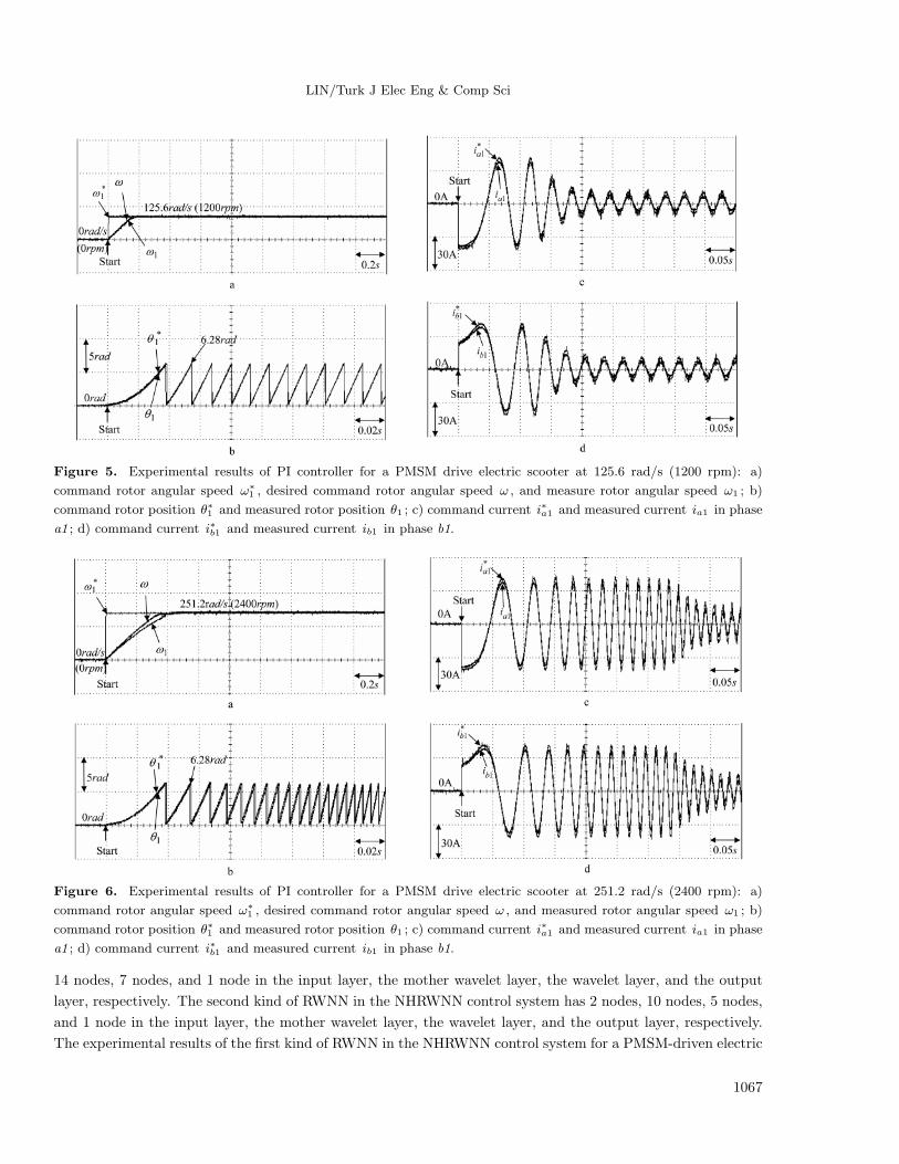
here, the first being the 125.6 rad/s (1200 rpm) caseand the second being the 251.2 rad/s (2400 rpm) case. Since

the electric scooter is a nonlinear time-varying system, the gains of the PI and PID controllers for the speed

tracking are obtained by trial-and-error in order to achieve good transient and steady-state control performance

in the 125.6 rad/s (1200 rpm) case. The control gains of the PI controller are KP = 12.5,KI = 1.2 in the

125.6 rad/s (1200 rpm) case for the speed tracking. The experimental results of the PI controller for a PMSM-

driven electric scooter for the 125.6 rad/s (1200 rpm) case are shown in Figure 5, where tracking responses of the

command rotor angular speed ω∗1 , the desired command rotor angular speed ω , and the measured rotor angular

speed ω1 are shown in Figure 5a; tracking responses of the command rotor position θ∗1 and the measured rotor

position θ1 are shown in Figure 5b; tracking responses of the command current i∗a1 and the measured current ia1

in phase a1 are shown in Figure 5c; and tracking responses of the command current i∗b1 and measured current

ib1 in phase b1 are shown in Figure 5d. The experimental results of the PI controller for a PMSM-driven electric

scooter in the 251.2 rad/s (2400 rpm) case are shown in Figure 6, where tracking responses of the command

rotor angular speed ω∗1 , the desired command rotor angular speed ω , and the measured rotor angular speed ω1

are shown in Figure 6a; tracking responses of the command rotor position θ∗1 and the measured rotor position

θ1 are shown in Figure 6b; tracking responses of the command current i∗a1 and the measured current ia1 in

phase a1 are shown in Figure 6c; and tracking responses of the command current i∗b1 and measured current ib1

in phase b1 are shown in Figure 6d. The control gains of the PID controller are KP = 13.2,KI = 2.1,KD = 1.2

in the 125.6 rad/s (1200 rpm) case for the speed tracking. The experimental results of the PID controller for

a PMSM-driven electric scooter for the 125.6 rad/s (1200 rpm) case are shown in Figure 7, where tracking

responses of the command rotor angular speed ω∗1 , the desired command rotor angular speed ω , and the

measured rotor angular speed ω1 are shown in Figure 7a; tracking responses of the command rotor position

θ∗1 and the measured rotor position θ1 are shown in Figure 7b; tracking responses of the command current

i∗a1 and the measured current ia1 in phase a1 are shown in Figure 7c; and tracking responses of the command

current i∗b1 and measured current ib1 in phase b1 are shown in Figure 7d. The experimental results of the PID

controller for a PMSM-driven electric scooter in the 251.2 rad/s (2400 rpm) case are shown in Figure 8, where

tracking responses of the command rotor angular speed ω∗1 , the desired command rotor angular speed ω , and

the measured rotor angular speed ω1 are shown in Figure 8a; tracking responses of the command rotor position



current i∗b1 and measured current ib1 in phase b1 are shown in Figure 8d. The degenerate tracking responses in

Figures 6a and 8a result from the occurrence of parameter variation and external load disturbance. From the

experimental results, sluggish speed tracking is obtained for the PI- and PID-controlled PMSM-driven electric

scooter due to the weak robustness of the linear controller.

The control gains of the proposed NHRWNN control system are α = 0.1, β = 0.5, σ = 0.05. All

the gains in the NHRWNN control system are chosen to achieve the best transient control performance in

experimentation considering the requirement of stability. For testing performance, the RWNN is adopted in the

4-layer structure with different nodes in the input layer, the mother wavelet layer, the wavelet layer, and the

output layer. The initialization of the wavelet network parameters in [36] is adopted to initialize the parameters

of the wavelets. The effect due to inaccurate selection of the initialized parameters can be retrieved by the

on-line parameter training methodology. The parameter adjustment process remains continually active for the

duration of the experimentation. For testing performance for the 4-layer RWNN with different nodes, 2 different

nodes are provided in experimentation. The first kind of RWNN in the NHRWNN control system has 2 nodes,

1066


Figure 5. Experimental results of PI controller for a PMSM drive electric scooter at 125.6 rad/s (1200 rpm): a)

command rotor angular speed ω∗1 , desired command rotor angular speed ω , and measure rotor angular speed ω1 ; b)

command rotor position θ∗1 and measured rotor position θ1 ; c) command current i∗a1 and measured current ia1 in phase

a1 ; d) command current i∗b1 and measured current ib1 in phase b1.

Figure 6. Experimental results of PI controller for a PMSM drive electric scooter at 251.2 rad/s (2400 rpm): a)

command rotor angular speed ω∗1 , desired command rotor angular speed ω , and measured rotor angular speed ω1 ; b)



14 nodes, 7 nodes, and 1 node in the input layer, the mother wavelet layer, the wavelet layer, and the output

layer, respectively. The second kind of RWNN in the NHRWNN control system has 2 nodes, 10 nodes, 5 nodes,

and 1 node in the input layer, the mother wavelet layer, the wavelet layer, and the output layer, respectively.

The experimental results of the first kind of RWNN in the NHRWNN control system for a PMSM-driven electric

1067


Figure 7. Experimental results of PID controller for a PMSM drive electric scooter at 125.6 rad/s (1200 rpm): a)

command rotor angular speed ω∗1 , desired command rotor angular speed ω , and measure rotor angular speed ω1 ; b)



Figure 8. Experimental results of PID controller for a PMSM drive electric scooter at 251.2 rad/s (2400 rpm): a)

command rotor angular speed ω∗1 , desired command rotor angular speed ω , and measured rotor angular speed ω1 ; b)



scooter in the 125.6 rad/s (1200 rpm) case are shown in Figure 9, where tracking responses of the command

rotor angular speed ω∗1 , the desired command rotor angular speed ω , and the measured rotor angular speed ω1

are shown in Figure 9a; tracking responses of the command rotor position θ∗1 and the measured rotor position

θ1 are shown in Figure 9b; tracking responses of the command current i∗a1 and the measured current ia1 in

1068


phase a1 are shown in Figure 9c; and tracking responses of the command current i∗b1 and measured current

ib1 in phase b1 are shown in Figure 9d. The experimental results of the first kind of RWNN in the NHRWNN

control system for a PMSM-driven electric scooter in the 251.2 rad/s (2400 rpm) case are shown in Figure 10,

where tracking responses of the command rotor angular speed ω∗1 , the desired command rotor angular speed

ω , and the measured rotor angular speed ω1 are shown in Figure 10a; tracking responses of the command rotor

position θ∗1 and the measured rotor position θ1 are shown in Figure 10b; tracking responses of the command

current i∗a1 and the measured current ia1 in phase a1 are shown in Figure 10c; and tracking responses of the

command current i∗b1 and measured current ib1 in phase b1 are shown in Figure 10d. The experimental results

of the second kind of RWNN in the NHRWNN control system for a PMSM-driven electric scooter in the 125.6

rad/s (1200 rpm) case are shown in Figure 11, where tracking responses of the command rotor angular speed

ω∗1 , the desired command rotor angular speed ω , and the measured rotor angular speed ω1 are shown in Figure

11a; tracking responses of the command rotor position θ∗1 and the measured rotor position θ1 are shown in

Figure 11b; tracking responses of the command current i∗a1 and the measured current ia1 in phase a1 are

shown in Figure 11c; and tracking responses of the command current i∗b1 and measured current ib1 in phase

b1 are shown in Figure 11d. The experimental results of the second kind of RWNN in the NHRWNN control

system for a PMSM-driven electric scooter in the 251.2 rad/s (2400 rpm) case are shown in Figure 12, where

tracking responses of the command rotor angular speed ω∗1 , the desired command rotor angular speed ω , and

the measured rotor angular speed ω1 are shown in Figure 12a; tracking responses of the command rotor position



current i∗b1 and measured current ib1 in phase b1 are shown in Figure 12d. However, owing to the on-line

adaptive mechanism of the RWNN and the compensated controller, accurate tracking control performance of

the PMSM can be obtained. These results show that the NHRWNN control system has better performances

Figure 9. Experimental results of the first kind of RWNN in the NHRWNN control system for a PMSM drive electric

scooter at 125.6 rad/s (1200 rpm): a) command rotor angular speed ω∗1 , desired command rotor angular speed ω , and

measured rotor angular speed ω1 ; b) command rotor position θ∗1 and measured rotor position θ1 ; c) command current

i∗a1 and measured current ia1 in phase a1 ; d) command current i∗b1 and measured current ib1 in phase b1.

1069


than the PI and PID controllers for speed perturbation for a PMSM-driven electric scooter. Additionally, the

small chattering phenomena that existed in phase a1 and in phase b1, as shown in Figures 10c, 10d, 12c, and

12d, are induced by on-line adjustment of the RWNN to cope with the high-frequency unmodeled dynamics of

the controlled plant.

Figure 10. Experimental results of the first kind of RWNN in the NHRWNN control system for a PMSM drive electric

scooter at 251.2 rad/s (2400 rpm): a) command rotor angular speed ω∗1 , desired command rotor angular speed ω , and

measured rotor angular speed ω1 ; b) command rotor position θ∗1 and measured rotor position θ1 ; c) command current

i∗a1 and measured current ia1 in phase a1 ; d) command current i∗b1 and measured current ib1 in phase b1.

Figure 11. Experimental results of the second kind of RWNN in the NHRWNN control system for a PMSM drive

electric scooter at 125.6 rad/s (1200 rpm): a) command rotor angular speed ω∗1 , desired command rotor angular speed

ω , and measured rotor angular speed ω1 ; b) command rotor position θ∗1 and measured rotor position θ1 ; c) command

current i∗a1 and measured current ia1 in phase a1 ; d) command current i∗b1 and measured current ib1 in phase b1.

1070


Figure 12. Experimental results of the second kind of RWNN in the NHRWNN control system for a PMSM drive

electric scooter at 251.2 rad/s (2400 rpm): a) command rotor angular speed ω∗1 , desired command rotor angular speed

ω , and measured rotor angular speed ω1 ; b) command rotor position θ∗1 and measured rotor position θ1 ; c) command

current i∗a1 and measured current ia1 in phase a1 ; d) command current i∗b1 and measured current ib1 in phase b1.

Figure 13. Experimental results due to a TL1 = 2 Nm load torque disturbance with load and shed load at 251.2 rad/s

(2400 rpm): a) command rotor angular speed ω∗1 , measured rotor angular speed ω1 , and measured current ia1 in phase

a1 using PI controller; b) command rotor angular speed ω∗1 , measured rotor angular speed ω1 , and measured current ia1

in phase a1 using PID controller; c) command rotor angular speed ω∗1 , measured rotor angular speed ω1 , and measured

current ia1 in phase a1 using the first kind of RWNN in the NHRWNN control system; d) command rotor angular speed

ω∗1 , measured rotor angular speed ω1 , and measured current ia1 in phase a1 using the second kind of RWNN in the

NHRWNN control system.

1071


The measured rotor speed responses due to step disturbance torque are given finally. The PI, PID,and NHRWNN methods are tested at TL1 = 2Nm load torque disturbance with load and shed load. The

experimental results due to a TL1 = 2Nm load torque disturbance with load and shed load at 251.2 rad/s (2400

rpm) are shown in Figure 13, where the measured rotor speed responses and measured current in phase a1

using the PI controller are shown in Figure 13a; the measured rotor speed responses and measured current inphase a1 using the PID controller are shown in Figure 13b; the measured rotor speed responses and measuredcurrent in phase a1 using the first kind of RWNN in the NHRWNN control system are shown in Figure 13c; andthe measured rotor speed responses and measured current in phase a1 using the second kind of RWNN in theNHRWNN control system are shown in Figure 13d. From the experimental results, the degenerated responsesdue to the variation of rotor inertia and load torque disturbance are much improved using the NHRWNN controlsystem. From experimental results, transient response of the NHRWNN control system is better than that ofthe PI and PID control systems at load regulation.

3. Conclusions

A PMSM drive system controlled by a NHRWNN control system has been successfully developed to drivean electric scooter with robust control characteristics. First, the dynamic models of the PMSM drive systemwere derived according to the electric scooter. Since the electric scooter is a nonlinear time-varying system,sluggish speed tracking was obtained for the PI- and PID-controlled PMSM-driven electric scooter due to theweak robustness of the linear controller. Therefore, to ensure the control performance of robustness, a PMSMcontrolled by the NHRWNN control system was developed to drive the electric scooter. The NHRWNN controlsystem with supervised control based on the uncertainty bounds of the controlled system was designed tostabilize the system states around a predetermined bound area. To drop the excessive chattering that resultedfrom the control efforts, the NHRWNN control system, which is composed of the supervised control, the RWNN,and the compensated control, was proposed to reduce and smooth the control effort when the system statesare inside the predetermined bound area. Moreover, an on-line parameter training methodology was derivedby using the Lyapunov stability theorem and the gradient descent method to increase the on-line learningcapability of the RWNN. From the experimental results, the control performance of the proposed NHRWNNcontrol system is more suitable than that of PI and PID controllers for a PMSM-driven electric scooter.

Acknowledgments

The author would like to acknowledge the financial support of the National Science Council of Taiwan, R.O.C.,through its grant NSC 99-2221-E-239-040-MY3.

Nomenclature

vd1, vq1 d-axis and q -axis stator voltages

id1, iq1 d-axis and q -axis stator currents

Ld1, Lq1 d-axis and q -axis stator inductances

R1 stator resistance

ω∗1 , ω, ω1 command rotor angular speed, desired

command rotor angular speed, rotor

angular speed

P1 number of poles

TL1 load torque (external load disturbance,

e.g., electric scooter)

B1 viscous frictional coefficient

J1 moment of inertia

λd d-axis flux linkage

Lm1 mutual inductance

Ifd1 d-axis magnetizing current

Tm electromagnet torque

Ke torque constant

i∗q1 q -axis command current

AH , BH , CH constants

LU1 (ω1) known continuous function

θf , θ∗1 , θ1 rotor flux position, command rotor

position, rotor position

LU2 , L3 known constants

e1 tracking error

UH , U∗H control law, ideal control law

ka positive constants

U1S , U2R, U3C supervised control, recurrent

wavelet neural network control,

compensated control

1072


V1, V2 Lyapunov functions

V1 positive constant

Ω(t) negative derivative of Lyapunov function

c1i , c2i , c

3j , c

4k inputs of nodes in the input layer, mother

wavelet layer, wavelet layer, output layer

of the recurrent wavelet neural network

g1i , g2j , g

3k, g

4o activation functions in the input layer,

mother wavelet layer, wavelet layer,

output layer of the recurrent wavelet

neural network

nod1i , nod2j ,

nod3k,nod4o node functions in the input layer,

mother wavelet layer, wavelet

layer, output layer of the recurrent

wavelet neural network

d1i , d2j , d

3k, d

4o outputs of nodes in the input layer,

mother wavelet layer, wavelet layer,

output layer of the recurrent wavelet

neural network

N number of iterations

sgn( ·) sign function

aij , bij translations and dilations

µ3jk, µ

4ko, µoi connective weights between the mother

wavelet layer and the wavelet layer,

connective weights between the wavelet

layer and the output layer, recurrent

weights for the units in the output layer

n, l1 total number of the wavelets with

respect to the input nodes, number of

wavelets if each input node has

the same mother wavelet nodes

∂V2/∂U2R Jacobian term of controlled system

θ(x) first derivative of the Gaussian wavelet

function

ψ collection vector of the adjustable

parameters of recurrent wavelet neural

network

χ input vector of the output layer of the

recurrent wavelet neural network

σ minimum approximation error

ψ∗ optimal weight vector that achieves the

minimum approximation error

υ2j , υ3k error term of mother wavelet function,

error term of mother layer

α, β small positive constant and adaptation

gain

ψ adaptation laws of the recurrent wavelet

neural network

i∗a1, i∗b1 command current in phase a1, command

current in phase b1

ia1, ib1 measure current in phase a1, measure

current in phase b1

References

[1] D.W. Novotny, T.A. Lipo, Vector Control and Dynamics of AC Drives, New York, Oxford University Press, 1996.

[2] W. Leonhard, Control of Electrical Drives, Berlin, Springer-Verlag, 1996.

[3] F.J. Lin, “Real-time IP position controller design with torque feedforward control for PM synchronous motor”,

IEEE Transactions on Industrial Electronics, Vol. 4, pp. 398–407, 1997.

[4] K.S. Narendra, K. Parthasarathy, “Identification and control of dynamical system using neural networks”, IEEE

Transactions on Neural Networks, Vol. 1, pp. 4–27, 1990.

[5] Y.M. Park, M.S. Choi, K.Y. Lee, “An optimal tracking neuro-controller for nonlinear dynamic systems”, IEEE

Transactions on Neural Networks, Vol. 7, pp. 1099–1110, 1996.

[6] F.F.M. El-Sousy, “A vector-controlled PMSM drive with a continually on-line learning hybrid neural-network model-

following speed controller”, Journal of Power Electronics, Vol. 5, pp. 197–210, 2005.

[7] C.H. Lin, “Switched reluctance motor drive for electric motorcycle using HFNN controller”, 7th International

Conference on Power Electronics and Drive Systems, pp. 1383–1388, 2007.

[8] S.S. Ge, C. Yang, T.H. Lee, “Adaptive predictive control using neural network for a class of pure-feedback systems

in discrete time”, IEEE Transactions on Neural Networks, Vol. 19, pp. 1599–1614, 2008.

1073

http://dx.doi.org/10.1007/978-3-642-97646-9

http://dx.doi.org/10.1109/72.80202

http://dx.doi.org/10.1109/72.80202

http://dx.doi.org/10.1109/72.536307

http://dx.doi.org/10.1109/72.536307


[9] M. Ghariani, I.B. Salah, M. Ayadi, R. Neji, “Neural induction machine observer for electric vehicle applications”,

International Review of Electrical Engineering, Vol. 3, pp. 314–324, 2010.

[10] P. Brandstetter, M. Kuchar, I. Neborak , “Selected applications of artificial neural networks in the control of AC

induction motor drives”, International Review of Electrical Engineering, Vol. 4, pp. 1084–1093, 2011.

[11] Q. Zhang, A. Benveniste, “Wavelet networks”, IEEE Transactions on Neural Networks, Vol. 3, pp. 889–898, 1992.

[12] B. Delyon, A. Juditsky, A. Benveniste, “Accuracy analysis for wavelet approximations”, IEEE Transactions on

Neural Networks, Vol. 6, pp. 332–348, 1995.

[13] J. Zhang, G.G. Walter, Y. Miao, W.N.W. Lee, “Wavelet neural networks for function learning”, IEEE Transactions

on Signal Processing, Vol. 43, pp. 1485–1496, 1995.

[14] J. Xu, D. W.C. Ho, D. Zhou, “Adaptive wavelet networks for nonlinear system identification”, Proceedings of the

American Control Conference, pp. 3472–3473, 1997.

[15] C.F. Chen, C.H. Hsiao, “Wavelet approach to optimizing dynamic systems”, IEE Proceedings on Control Theory

and Applications, Vol. 146, pp. 213–219, 1999.

[16] N. Sureshbabu, J.A. Farrell, “Wavelet-based system identification for nonlinear control”, IEEE Transactions on

Automatic Control, Vol. 44, pp. 412–417, 1999.

[17] Z. Zhang, C. Zhao, “A fast learning algorithm for wavelet network and its application in control”, Proceedings of

IEEE International Conference on Control Automation, pp. 1403–1407, 2007.

[18] S.A. Billings, H.L. Wei, “A new class of wavelet networks for nonlinear system identification”, IEEE Transactions

on Neural Networks, Vol. 16, pp. 862–874, 2005.

[19] D. Giaouris, J.W. Finch, O.C. Ferreira, R.M. Kennel, G.M. El-Murr, “Wavelet denoising for electric drives”, IEEE

Transactions on Industrial Electronics, Vol. 55, pp. 543–550, 2008.

[20] R.H. Abiyev, O. Kaynak, “Fuzzy wavelet neural networks for identification and control of dynamic plants—a novel

structure and a comparative study”, IEEE Transactions on Industrial Electronics, Vol. 55, pp. 3133–3140, 2008.

[21] D. Gonzalez, J.T. Bialasiewicz, J.Balcells, J. Gago, “Wavelet-based performance evaluation of power converters

operating with modulated switching frequency”, IEEE Transactions on Industrial Electronics, Vol. 55, pp. 3167–

3176, 2008.

[22] F.J. Lin, R.J. Wai, M.P. Chen, “Wavelet neural network control for linear ultrasonic motor drive via adaptive

sliding-mode technique”, IEEE Transactions on Ultrasonics, Ferroelectrics, and Frequency Control, Vol. 50, pp.

686–697, 2003.

[23] S.H. Ling, H.H.C. Iu, F.H.F. Leung, K.Y. Chan, “Improved hybrid particle swarm optimized wavelet neural

network for modeling the development of fluid dispensing for electronic packaging”, IEEE Transactions on Industrial

Electronics, Vol. 55, pp. 3447–3460, 2008.

[24] G. Gokmen, “Wavelet based instantaneous reactive power calculation method and a power system application

sample”, International Review of Electrical Engineering, Vol. 4, pp. 745–752, 2011.

[25] K. Funahashi, Y. Nakamura, “Approximation of dynamical systems by continuous time recurrent neural network”,


[26] L. Jin, P.N. Nikiforuk, M. Gupta, “Approximation of discrete-time state-space trajectories using dynamic recurrent

networks”, IEEE Transactions on Automatic Control, Vol. 6, pp. 1266–1270, 1995.

[27] C.C. Ku, K.Y. Lee, “Diagonal recurrent neural networks for dynamical system control”, IEEE Transactions on


[28] F.J. Lin, R.J. Wai, C.M. Hong, “Hybrid supervisory control using recurrent fuzzy neural network for tracking

periodic inputs”, IEEE Transactions on Neural Networks, Vol. 12, pp. 68–90, 2001.

[29] C.H. Lu, C.C. Tsai, “Adaptive predictive control with recurrent neural network for industrial processes: an

application to temperature control of a variable-frequency oil-cooling machine”, IEEE Transactions on Industrial

Electronics, Vol. 55, pp. 1366–1375, 2008.

1074

http://dx.doi.org/10.1109/72.165591

http://dx.doi.org/10.1109/72.363469

http://dx.doi.org/10.1109/72.363469

http://dx.doi.org/10.1109/78.388860

http://dx.doi.org/10.1109/78.388860

http://dx.doi.org/10.1049/ip-cta:19990516

http://dx.doi.org/10.1049/ip-cta:19990516

http://dx.doi.org/10.1109/9.746278

http://dx.doi.org/10.1109/9.746278

http://dx.doi.org/10.1109/TNN.2005.849842

http://dx.doi.org/10.1109/TNN.2005.849842

http://dx.doi.org/10.1109/TIE.2007.911943










http://dx.doi.org/10.1016/S0893-6080(05)80125-X

http://dx.doi.org/10.1016/S0893-6080(05)80125-X





[30] S.J. Yoo, J.B. Park, Y.H. Choi, “Stable predictive control of chaotic systems using self-recurrent wavelet neural

network”, International Journal of Automatic Control Systems, Vol. 3, pp. 43–55, 2005.

[31] C.H. Lu, “Design and application of stable predictive controller using recurrent wavelet neural networks”, IEEE

Transactions on Industrial Electronics, Vol. 56, pp. 3733–3742, 2009.

[32] C.H. Lin, C.P. Lin, “The hybrid RFNN control for a PMSM drive system using rotor flux estimator”, International

Conference on Power Electronics and Drive Systems, pp. 1394–1399, 2009.

[33] C.H. Lin, P.H. Chiang, C.S. Tseng, Y.L. Lin, M.Y. Lee, “Hybrid recurrent fuzzy neural network control for

permanent magnet synchronous motor applied in electric scooter”, International Power Electronics, pp. 1371–1376,

2010.

[34] J.J.E. Slotine, W. Li, Applied Nonlinear Control, Englewood Cliffs, NJ, USA, Prentice Hall, 1991.

[35] K.J. Astrom, B. Wittenmark, Adaptive Control, New York, Addison-Wesley, 1995.

[36] Y.Oussar, G. Dreyfus, “Initialization by selection for wavelet network training”, Neurocomputing, Vol. 34, pp.

131–143, 2000.

1075

http://dx.doi.org/10.1016/S0925-2312(00)00295-2

http://dx.doi.org/10.1016/S0925-2312(00)00295-2

A novel hybrid recurrent wavelet neural network control of ...

Documents

Transcript of A novel hybrid recurrent wavelet neural network control of ...