Combustion and Flame 160 (2013) 909–919

Contents lists available at SciVerse ScienceDirect

Combustion and Flame

journal homepage: www.elsevier .com/locate /combustflame

A novel framework for the quantitative analysis of high resolutiontransmission electron micrographs of soot I. Improved measurementof interlayer spacing

0010-2180/$ - see front matter Published by Elsevier Inc. on behalf of The Combustion Institute.http://dx.doi.org/10.1016/j.combustflame.2013.01.002

⇑ Corresponding author.E-mail address: toth.pal@uni-miskolc.hu (P. Toth).

Pal Toth a,⇑, Arpad B. Palotas b, Eric G. Eddings a, Ross T. Whitaker c, JoAnn S. Lighty a

a Department of Chemical Engineering, University of Utah, 50 S. Central Campus Drive, Salt Lake City, UT 84112-9203, United Statesb Department of Combustion Technology and Thermal Energy, University of Miskolc, H3515 Miskolc-Egyetemvaros, Hungaryc School of Computing, University of Utah, 3893 Warnock Engineering Building, Salt Lake City, UT 841112-9205, United States

a r t i c l e i n f o a b s t r a c t

Article history:Received 27 October 2012Received in revised form 8 January 2013Accepted 8 January 2013Available online 6 February 2013

Keywords:SootNanostructureHRTEM

The reliable and reproducible quantitative image analysis of digital micrographs from high resolutiontransmission electron microscopy (HRTEM) of soot has been an area of interest since the early nineties.Since the resolution of HRTEM images is usually sufficient to carry out structural measurements at theatomic level, the information obtained from these images is very valuable as it potentially yields insightinto very specific soot oxidation processes; however, extracting physically meaningful, reliable, accurateand statistically robust data from HRTEM images is not an easy process. Data extraction is hindered bythe presence of overlapping structures, varying focus, contrast, illumination levels and noise in theimages. In this paper a novel image analysis framework is presented to address these issues and explorethe possibility of the extraction of high-fidelity structural data from HRTEM soot images. Emphasis is onthe analysis of images of mostly amorphous, poorly ordered soot structures, as these are the most diffi-cult to analyze.

Published by Elsevier Inc. on behalf of The Combustion Institute.

1. Introduction

The digital image analysis of high resolution transmission elec-tron microscopy (HRTEM) images of soot allows for the character-ization of the carbon structure at the atomic level. The nanoscaleobservation of soot structure is motivated by either an incentiveto determine the source of soot pollution [1,2] or to better under-stand combustion processes [3]. A typical soot HRTEM micrographshows an overlapping pattern of periodically occurring dark andbright lines of varying orientation and contrast. These lines are alsocalled fringes and they are understood to be projections of graph-ene layers formed by phase contrast imaging principles. The mean-ing of dark and bright fringes are not obvious, as depending on theimaging conditions, they can either indicate carbon atoms or thespaces between them. Although not typical, the meaning of brightand dark fringes can be also dynamically reversed depending onimaging conditions and sample thickness. This phenomenon willbe referred to as phase inversion in this paper. Also, it is practicallyimportant to satisfy some general conditions for the reliable mea-surement of geometric properties of fringe images: first, fringecontrast should be maximized and second, image regions where

fringe contrast changes abruptly should not be used for geometricanalysis [4]. Image processing and analysis methods aiming to ex-tract structural information from HRTEM images of soot have beendeveloped and applied since the mid-nineties [5–10]. These meth-ods differ in details, however the basic procedure consists of thefollowing steps:

1. The pre-filtering of the digital micrograph. This step usuallyconsists of frequency filtering; i.e., the removal of unwantedfrequencies in the image. Since carbon layers can only appearin a well-known frequency band determined by physicallymeaningful values of their interlayer spacing, bandpass fre-quency filtering is ideal for noise reduction in HRTEM sootimages.

2. The detection of separate fringes. This step is usually an imagebinarization procedure, meaning that the initially gray scaleimage is transformed to a binary image in which fringes areindicated as 1 values and background is indicated by 0 values.Until lately, in most cases this transformation has been a global,non-adaptive binarization process; i.e., a single pixel intensitythreshold has been set to determine whether a particular pixelbelongs to a fringe or background. Authors have started toreport results obtained by methods utilizing adaptive binariza-tion [10]. The outcome of this step is a binary image in whichindividual objects (fringes) can be detected and labeled.

910 P. Toth et al. / Combustion and Flame 160 (2013) 909–919

3. The postprocessing of binary objects. In this step, the labeledbinary fringes are processed further. The postprocessing tech-niques vary from author to author. Some use geometric criteriafor selecting valid fringe candidates [5], some use skeletoniza-tion algorithms to reduce fringes to curves or line segments[6–10] and some implement fringe separation/reconnectionlogic [7].

4. The data extraction step. In this step geometric information isextracted from the postprocessed binary fringe objects. Geo-metric data can include fringe lengths [6–10], fringe tortuosity[9,10], fringe separation (interlayer distance) [5–10] and fringeorientation [5,8], among others.

The obtained geometrical data is in the form of vectors or sets ofthe mentioned properties. Each value in each set corresponds to aparticular detected fringe in the analyzed micrograph. After extrac-tion, these sets can be statistically described by constructing prob-ability distribution functions (PDFs), specifying mean and standarddeviation values and so forth. Structural order can be characterizedby quantifying the symmetries and deviations in fringe orientationor fringe spacing values [6,8]. The common drawbacks of method-ologies that are based on the steps described above are the usage ofsubjectively set image processing parameters, results that are sen-sitive to these parameters and the insufficient amount of structuraldata extracted due to the oversimplification of images (the detec-tion and artificial separation of individual fringes). Because of allthese reasons, it is understood that the quantitative characteriza-tion and differentiation of real soot HRTEM images can be a diffi-cult problem, especially when trying to differentiate poorlyordered, highly amorphous and/or only slightly different samples.In fact, the quantitative image analysis of amorphous soot sampleshas been considered an unsolved problem since the publication ofthe first papers in this area, especially when on aims to measureinterlayer spacing statistics in soot structures (e.g., see insufficientnumber of data points in [11] or insignificant differences in statis-tics in [12]). Recently, we have developed an image analysis proce-dure with which distances can be measured between curvedgraphene layers as well, thus increasing the fidelity of the obtaineddistributions; however, this method does not avoid the subjectivityof binarization techniques and can only be used to obtain semi-quantitative descriptors [13].

1 In other words, signals.

2. Materials and methods

In this section a detailed description of the proposed image pro-cessing and analysis methodology is given along with the detailsand origins of the image sets used for the validation and verifica-tion of the proposed algorithm.

2.1. Image analysis procedure – overview

The image processing methodology proposed in this work iscompletely different from the methods discussed in Section 1.The proposed method has been developed to address and over-come all the specific issues of the standard methods and it utilizesrecent advances and ideas from the image analysis and signal pro-cessing literature. Similar algorithms have been applied in HRTEMcrystallography [14,15]. While these published algorithms are sim-ilar, they are not applicable to images of more complex nanostruc-tures. The basic objectives of the proposed methodology are thefollowing:

1. To extract as much structural data as possible from a singlemicrograph. A higher number of data points means more accu-rate and reliable statistical evaluation of the structure. Being

able to extract the highest amount of structural informationfrom a single image has significant importance in cases wherethe availability of samples or micrographs is limited. Since typ-ical procedures for soot sampling deposit abundant quantitiesof soot particles on TEM grids, the scarcity of samples is usuallynot a problem when analyzing real soot. However, dependingon the heterogeneity of the soot particles, acquiring and analyz-ing a number of micrographs that is sufficient for obtainingrobust statistics can be a time-consuming process. In thesecases, being able to extract as much information as possiblefrom each micrograph not only increases the fidelity of theresults, but has practical and economic importance as well.

2. To extract information only from reliable image regions in orderto minimize measurement uncertainty and errors.

3. To measure structural parameters as accurately as possible.4. To minimize the number and effect of subjectively chosen and

set image processing parameters that are purely technical anddo not hold any real physical meaning (e.g., threshold values,filter kernel sizes and parameters for fringe detection logic –see [5] or [11] for typically arising parameters).

5. To be able to handle typical aberrations and artifacts present inHRTEM micrographs; e.g., noise, inhomogeneous illuminationand phase inversion.

To achieve these objectives, one must consider a different mod-el for soot HRTEM images than the standard model. By image mod-el we refer to a mindset that is used to interpret these images. Thestandard model assumes that the micrographs contain identifiableor detectable objects; – i.e., imaged physical bodies (atoms or lay-ers of atoms) with well defined boundaries and the standard meth-ods aim to locate these bodies and their boundaries in the images.Such a model inherently leads to large amounts of eliminated data,as it is only interested in the detected bodies themselves (whichare well defined and quantized) and their geometric properties. In-stead, our approach interprets the micrographs as continuous (atleast at the image level) projections of patterns in electromagneticfields1 and tries to analyze the patterns evolved in the projections.This image model is also more realistic from the quantum-physicalpoint of view. Mathematically, images are interpreted as superposi-tions of two-dimensional patches of sinusoidal patterns with varyingphase, frequency, amplitude and orientation corrupted by noise andcontrast inhomogeneity. The proposed parameters to use for struc-tural characterization are exactly these (and the maps of these) sig-nal properties. It is easy to see that, following the proposed imagemodel, there is no need for a detection step; – i.e., the labeling ofwell-defined binary fringes. Information can be extracted at the na-tive resolution of the image, meaning that every single pixel in theimage will yield a set of structural parameters. The approach resultsin an abundant flow of information, which contributes to the statis-tical robustness of the extracted data. It is also possible to evaluatecertain image regions based on their quality (signal strength) andonly extract structural information from reliable regions. Since theapproach is a spectral technique and is not based on pixel-levelmanipulations, sub-pixel accuracy can be achieved in the measure-ment of structural parameters. The upper limit of pointwise accuracyof these measurement is only set by the Nyquist sampling criterion.In the following, a detailed description of the methodology and ap-proach is given.

2.2. Image analysis procedure – development

Three structural parameters are proposed in this study. Theseare the local orientation h, local wavelength k and local modulation

2 Here the symbols represent an interval that is open from the left and closed from

P. Toth et al. / Combustion and Flame 160 (2013) 909–919 911

strength l of the signal. These describe the sinusoidal pattern in aspecific location in the image, but since the sinusoidal patterns arein fact the interpretations of fringes, the proposed structural prop-erties are simply the continuous generalized versions of the al-ready used and published fringe structural parameters. Moreprecisely, local orientation is a generalized version of fringe orien-tation and local wavelength is the generalized version of the inter-layer spacing. The local modulation strength is a new parameterthat describes and quantifies the reliability and local anisotropyof the neighborhood around a specific pixel. To extract these gen-eralized structural parameters, a localized frequency filtering ap-proach is applied based on filtering the images with a set ofGabor filters, also called a Gabor filter bank. Several similar algo-rithms have been proposed in the field of medical image process-ing and computer vision for applications like image registration[16,17]. The general approach is a hybrid spatial/frequency domainfiltering method and it combines the advantages (sub-pixel resolu-tion, spectral representation and localization) of both [18]. Gaborfilters are quadrature filters that can be fine-tuned to specificwavelengths, scales and orientations. Filtering (mathematicallyrealized by two-dimensional convolution) the image with a Gaborfilter yields a filtered image, also called a response. In this re-sponse, locations where the wavelength and orientation of thesinusoidal pattern in the original image were the closest to thewavelength and orientation of the Gabor filter yield the highest re-sponse value. Thus, by repeatedly filtering the image with a set ofdifferently tuned Gabor filters and recording the responses, it ispossible to extract local wavelength and orientation values at eachimage pixel. The term quadrature refers to the phase-independentresponse magnitudes of Gabor filtering. Since the phase of a sinu-soidal pattern is directly connected to its local intensity, it is easyto see that Gabor filtering analysis is immune to the phase inver-sion phenomenon mentioned in Section 1. In other words, it isnot important whether dark or bright pixels indicate atoms orspaces between atoms – the responses will be the same in bothdark and bright regions. Gabor filters also achieve the theoreticallowest localization uncertainty, thus they are ideal candidates forapplications where one aims to minimize measurement uncertain-ties [19,20]. The analytical form of a two-dimensional Gabor filterin the spatial domain is the following:

gðx; yÞ ¼ 12prxry

exp � x02

2r2x� y02

2r2y

!exp

2pix0

gk

� �¼Wðx; yÞSðx; yÞ

ð1Þ

By definition, the two-dimensional (x, y) spatial Gabor filter is asuperposition of a Gaussian window W(x, y) and a complex sinu-soidal S(x, y). rx is the scale parameter of the Gaussian windowin the x direction and ry is the scale parameter of the Gaussianwindow in the y direction. i is the complex unit vector and gk isthe wavelength of the complex sinusoidal (in other words, thewavelength to which the filter is tuned to). The rotated coordinatesx0 and y0 can be expressed as

x0 ¼ x cosðghÞ þ y sinðghÞ ð2Þy0 ¼ y cosðghÞ � x sinðghÞ ð3Þ

where gh is the orientation angle to which the filter is tuned to. gk

and gh are not the same as the local wavelength k and orientationh of the image at a particular pixel, thus the different notation.The frequency domain form of the Gabor filter is a Gaussian surface.It can be written as the Fourier transform of g(x, y):

Gðu; vÞ ¼ F½gðx; yÞ� ¼ expr2

x ð2pþ gku0Þ2

2g2k � 0:5ðv 0ryÞ2

!ð4Þ

where u and v are the horizontal and vertical frequency coordinates,respectively. u0 and v0 are rotated frequency coordinates and are ob-tained similarly to x0 and y0. F denotes Fourier transformation withrespect to a centrally shifted frequency domain (u, v). A quadratureGabor filter pair along with its frequency domain representation isshown in Fig. 1.

The filter demonstrated in Fig. 1 is only a single member of thefilter bank that is used to extract wavelengths and orientationsfrom the image. The design of the whole filterbank is the most prac-tical to carry out in the frequency domain. The general idea behindthe filter bank design is to cover and sample the relevant frequencybands of the image with Gabor filters. The filter bank is therefore acollection of sets of filter parameters gh, gk, rx, ry and by the designof the filter bank, one refers to the determination of these parame-ters. The determination of gh and gk is an easier process, since typ-ical HRTEM soot images contain orientations in the full range[�p/2, p/2[2 and wavelengths corresponding to a well defined fre-quency band derived from valid interlayer spacing values. One thingto note is that while the orientation scale is linear, the frequency (andtherefore wavelength) scale is not, thus one must sample wave-lengths exponentially (lower frequencies/higher wavelengths mustbe sampled more densely). Also note that due to the direction ambi-guity of orientation angles, h values only cover a half circle (a range ofp). In other words, an orientation angle value of h1 means exactly thesame orientation as h1 ± lp, where l is an integer. One needs to specifya number of filters nh to cover the range of h and another number nk tocover the range of k. Once these numbers are specified, the orienta-tion and wavelength values to sample can be calculated as

gh;j ¼ �p2þ j

pnh

ð5Þ

gk;k ¼ kminqk�1 ð6Þ

q ¼ kmin

kmax

� �� 1nk�1

ð7Þ

where j and k are indices of positive integers between [1, nh] and [1,nk], respectively; hj is the jth orientation, kk is the kth wavelength,kmin is the lowest wavelength (highest frequency) of interest andkmax is the highest wavelength (lowest frequency) of interest. Thepermutation of the sets of gh,j and gk,k obtained in this way mapsout the filter center frequencies in the frequency domain. Afterthese center frequencies are found, one still needs to specify thescale parameters rx and ry of each filter. The idea behind the spec-ification of the scale parameters is that the value of adjacent filterscan be specified at a point equally far away from their center fre-quencies. Since there are nh � nk possible permutations of sets ofgh,j and gk,k, nh � nk values of rx,j,k and ry,j,k must be specified. By fix-ing the filter values qh and pk at intermittent points between theircentral frequencies corresponding to the overlapping values in theh (angular) and k (radial) directions in the frequency domain, it isapparent that the scale parameter values can be determined bythe following relationships [21]:

rx;j;k ¼ 2p�i 1

gk;k� q

gk;k

� �ð1þ qÞ ln pkð Þð Þ1=2

0@

1A�1

ð8Þ

ry;j;k ¼0:5

2pi tan p

2nh

� �g�1

k;k

� �2ðlnðphÞÞ1=2

24

35

ð9Þ

Note that since the frequency responses of the Gabor filters arenormalized, both ph and pk must be less than 1. If this condition issatisfied, the above equations yield real values for scale parameters.

the right.

Fig. 1. From left to right: the real component of a Gabor filter in the spatial domain, the imaginary component (quadrature pair) of a Gabor filter in the spatial domain, theFourier transformed Gabor filter in the frequency domain. The parameters used are: gh = p/3, gk = 0.35 nm, rx = 0.25, ry = 0.5. This filter would give the highest response atlocations where fringes with a spacing of 0.35 nm oriented at p/3 radians are present in an image with a size of 200 � 200 pixels and a nm per pixel ratio of 5/150. Thefrequency domain filter is a Gaussian surface centered around frequencies (u0, v0). The Euclidean distance of this central point from the origo is exactly 1/gk. Note that thefilter shown here is enlarged for visualization purposes. Typical filters used for data extraction fit inside a 64 � 64 kernel window.

912 P. Toth et al. / Combustion and Flame 160 (2013) 909–919

It is also worth noting that the scale parameters are only functionsof gk,k and not gh,j, which is understandable since the orientationrange is sampled linearly. Figure 2 demonstrates the design andconstruction of a typical Gabor filter bank for soot HRTEM imageanalysis. Note that while the filter bank essentially contains param-eter sets of gh, gk, rx, ry, to calculate these sets, the set nk, nh, pk, ph

must be determined. Therefore, for the balance of this paper theset nk, nh, pk, ph will be referred to as the filter bank parameters.

To extract orientations and wavelengths, the HRTEM image isfiltered with each filter in the constructed filter bank. The responsevalues for each image pixel are recorded. Intuitively, one can deter-mine the orientation and wavelength at a specific pixel by identi-fying the filter which gave the highest response at that pixel. Theorientation and wavelength of the particular pixel can be esti-mated as the orientation and wavelength to which the identifiedbest filter is tuned to. While this method is intuitive and graphical,the resulting orientations and wavelengths will be heavily quan-tized depending on the sampling density of the filter bank. In orderto obtain continuous and smooth orientation and wavelengthmaps, an interpolation method is used in this study. The basic ideaof this technique is that the intermediate responses of the filterbank can be approximated by using the individual frequency re-sponses of the filters. The sum of individual filter responses,weighted by the discrete response values obtained by filtering,

Fig. 2. A demonstration of the design and construction of a Gabor filter bank. Left: HRTEtransformation, plotted on a logarithmic scale) of the soot image. Circles denote thewavelengths between 0.3 and 0.6 nm. These values are chosen based on a priori knowledautomatically by locating the frequency band containing the highest spectral energy (as ithe superimposed Gabor filters in the frequency domain. Crosses denote the center freqph = 0.05, pk = 0.05. Note that the filter bank shown in this figure was not the filter bank

very closely approximates the continuous response surface onewould obtain by filtering with a very densely spaced filter bank.In other words, the ideally high-resolution response surface canbe approximated by a finite number of filter responses. The errorsintroduced by this approximation have been quantified by Peronain 1991 [22]. It has been shown that the error of the approximationquickly approaches zero as the number of filters increases. For ourapplication, the error is practically negligible (approximately 1%) inh and k if one uses 15 or more filters per orientation and wave-length range. Mathematically, to find h and k at each pixel, oneneeds to find the global maximum of the interpolated responsesurface obtained by the following:

Ro ¼ ReðI � goÞ2 þ ImðI � goÞ

2� �1=2

����x0 ;y0

ð10Þ

Rðu; vÞ ¼Xnh�nk

o¼1

Goðu;vÞRo ð11Þ

ðumax; vmaxÞ ¼ arg maxu;v½Rðu;vÞ� ð12Þ

h ¼ p2þ tan�1ðvmax=umaxÞ ð13Þ

k ¼ u2max þ v2

max

� ��12 ð14Þ

l ¼ Rðumax;vmaxÞRidealðumax;vmaxÞ

ð15Þ

M image of a real soot sample. Middle: the power spectrum (magnitude of Fourierselected frequency band for further analysis. This frequency band corresponds toge of the physically meaningful interlayer spacing values for soot or can be selectedt is demonstrated by the bright ring around the origo). Right: gray scale values showuencies of the Gabor filters. The parameters of the filter bank are: nh = 10, nk = 10,that was used to extract the data that will be presented in Section 3.3.

P. Toth et al. / Combustion and Flame 160 (2013) 909–919 913

where R(u, v) is the interpolated (continuous) response surface at aparticular pixel (x0, y0), o is the linear index of filters in the filterbank, Go is the filter frequency response of the oth filter as it is givenby Eq. (4), Ro is the discrete response magnitude at a particular pixel(x0, y0) of the oth filter and (umax, vmax) is the frequency pair whichmaximizes R(u, v). I refers to the gray scale image itself, � is thesymbol of convolution, Re() means the real part of its argumentsand Im() means the imaginary part of its argument. The ideal max-imum filter response Rideal(u, v) refers to the theoretical maximumresponse at a location in the continuous interpolated response sur-face. This value is calculated by convolving an artificial image tem-plate containing a sinusoidal pattern oriented and spacedappropriately to a specific filter with maximum contrast and inten-sity (thus effectively a two-dimensional square-wave signal). Thisnormalization scales the modulation strength between 0 and 1and therefore makes it a good descriptor for comparing differentimages taken under similar imaging conditions. Note that it is pos-sible to scale the modulation strength by the maximum modulationstrength found in the particular image, making it an intensity-invariant structural parameter and allowing for the comparison ofimages taken under different imaging conditions. To find the globalmaximum, a local direct search algorithm has been applied [23].Global optimization algorithms are usually computationally inten-sive and difficult to implement, but the global maximum can bereliably found by local maximum search algorithms if the initialguess for the maximum is very close to the global maximum.Assuming a smooth and unimodal response surface, the center fre-quency of the filter that yielded the highest discrete response is avery good initial guess in this problem. The direct search algorithmhas been implemented by using Matlab’s fminsearch function. Fig-ure 3 demonstrates the maximum search step in the continuous re-sponse surface.

Thus the complete algorithm can be summarized as follows:

1. Load the image.2. Specify the wavelength band of interest either manually or

automatically based on the power spectrum.3. Calculate filter parameters by using Eqs. (5)–(9) and con-

struct the filter bank.4. Filter the image with each filter in the filter bank and record

the discrete responses at each pixel.5. At each pixel, calculate the frequencies that maximize the

continuous interpolated response surface using optimiza-tion and store these frequencies using Eqs. (10)–(12).

6. Calculate structural parameters h, k and l at each pixelusing Eqs. (13)–(15) and store.

While filtering can be realized by numerical convolution usingcomputationally inexpensive Fast Fourier Transforms (FFTs), thewhole algorithm represents a huge computational load due tosteps 5 and 6. To overcome this problem and keep the computa-tion times under reasonable limits, steps 5 and 6 have beenimplemented as parallel algorithms. Under a Matlab environmentusing a modern quad-core computer computations take 10–60 min, depending on the image and selected filter bank. Process-ing the typical HRTEM image shown in Fig. 2 took 17 min. If in aspecific application computation time is an issue, the algorithmcan be further optimized by only using discrete filter responsesin the close neighborhood of the filter with the maximum dis-crete response to compute R(u, v) in the frequency domain, man-ually specifying regions of interests (ROIs) or outsourcing parts ofthe computation to graphical processing units (GPUs) that arecommonly found in modern personal computers. Figure 4 demon-strates typical extracted fields of the three derived structuralparameters.

2.3. Soot sampling

Graphite materials (Union Carbide) from three different fuels(anthracene, bifluorenyl and p-terphenyl) were previously synthe-sized by high temperature (3000 �C) pyrolysis. The sample prepa-ration procedure has been reported earlier [1]. In brief, thesamples were ground in an agate mortar and pestle and then ultra-sonically dispersed in ethanol. The suspension was deposited drop-wise onto a copper TEM grid coated with a lacey carbon film.HRTEM micrographs of the carbon particles were obtained usinga transmission electron microscope operated at 200 keV. Amor-phous soot samples were taken using thermophoretic samplingmethods previously described in [3]. In brief, benzene was burnedin air under fuel rich conditions in a premixed flat flame burnerthat was initially developed for studying aliphatic and aromaticflames. This system consisted of a stainless steel chamber wherefuel and air were properly mixed prior to entering the burner.The flame was stabilized over a tube bundle and was shielded fromatmospheric interference using a nitrogen shroud. A metallic meshplaced 3.5 cm above the burner surface stabilized and distributedthe flame uniformly across the burner. Samples for HRTEM analysiswere taken at different heights above the burner surface (HAB)using a thermophoretic probe commonly referred to as a frog ton-gue. A TEM grid holder was attached to a piston and compressedair at 60 psig was used to quickly insert and remove the TEM gridfrom the flame. Multiple insertions were necessary to get a repre-sentative soot sample on the grid. The grid was oriented with theface parallel to the gas flow, so that the disturbance of the flamewas minimal. Soot deposits on the grid due to the thermophoreticgradient between the cold grid and the hot flame, which also al-lows freezing of some heterogeneous reactions, as well as avoidingchanges in the soot morphology after the particles have impactedupon the cold surface.

3. Results and discussion

To demonstrate the capabilities of the proposed algorithm, testswith both artificial and real images have been carried out. Testingwith artificial images is important, since it can achieve what test-ing with real data cannot: verification of the method by compari-son with accurately known ground truth. To demonstrate thatthe proposed method is capable of reproducing already publishedresults – with higher resolution and accuracy – results from a pa-per presenting standard structural analysis of different graphites[1] have been compared to results obtained by the method pre-sented here. In addition to demonstrate the methods capabilityof analyzing and differentiating poorly ordered soot structures, re-sults for images of immature soot obtained by standard imageanalysis methods and the method proposed here are compared [5].

3.1. Artificial images

Since the method proposed here is practically a signal analysisroutine with a number of features specifically designed for sootHRTEM image analysis, artificial images can be constructed to val-idate the algorithm and quantify its accuracy. Images showing asinusoidal pattern with varying orientation and wavelength havebeen generated by taking the sine of an underlying polynomialphase surface. The theoretical wavelength can be calculated asthe inverse of the phase gradient magnitude, while the theoreticalorientation can be calculated as the orientation angle of the gradi-ent. After generating the images, they have been artificially cor-rupted by zero-mean Gaussian noise. The standard deviation ofthe noise has been increased in steps in order to evaluate the algo-

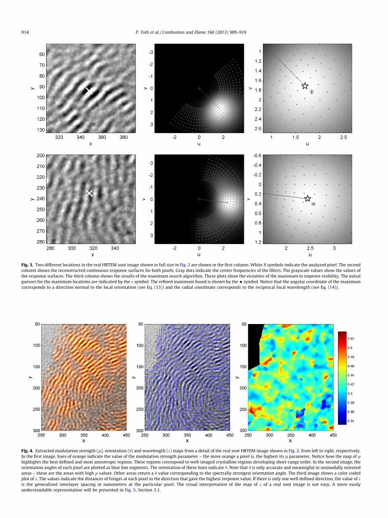
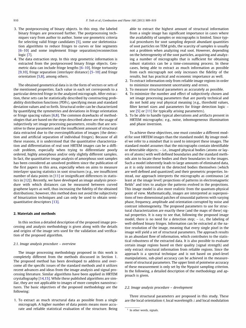
Fig. 3. Two different locations in the real HRTEM soot image shown in full size in Fig. 2 are shown in the first column. White X symbols indicate the analyzed pixel. The secondcolumn shows the reconstructed continuous response surfaces for both pixels. Gray dots indicate the center frequencies of the filters. The grayscale values show the values ofthe response surfaces. The third column shows the results of the maximum search algorithm. These plots show the vicinities of the maximum to improve visibility. The initialguesses for the maximum locations are indicated by the ⁄ symbol. The refined maximum found is shown by the w symbol. Notice that the angular coordinate of the maximumcorresponds to a direction normal to the local orientation (see Eq. (13)) and the radial coordinate corresponds to the reciprocal local wavelength (see Eq. (14)).

Fig. 4. Extracted modulation strength (l), orientation (h) and wavelength (k) maps from a detail of the real soot HRTEM image shown in Fig. 2, from left to right, respectively.In the first image, hues of orange indicate the value of the modulation strength parameter – the more orange a pixel is, the highest its l parameter. Notice how the map of lhighlights the best defined and most anisotropic regions. These regions correspond to well-imaged crystalline regions developing short-range order. In the second image, theorientation angles of each pixel are plotted as blue line segments. The orientation of these lines indicate h. Note that h is only accurate and meaningful in unimodally orientedareas – these are the areas with high l values. Other areas return a h value corresponding to the spectrally strongest orientation angle. The third image shows a color codedplot of k. The values indicate the distances of fringes at each pixel in the direction that gave the highest response value. If there is only one well defined direction, the value of kis the generalized interlayer spacing in nanometers at the particular pixel. The visual interpretation of the map of k of a real soot image is not easy. A more easilyunderstandable representation will be presented in Fig. 5, Section 3.1.

914 P. Toth et al. / Combustion and Flame 160 (2013) 909–919

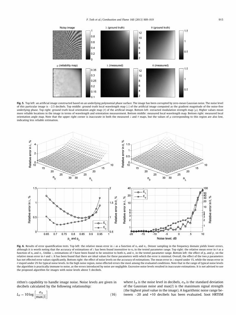
Fig. 5. Top left: an artificial image constructed based on an underlying polynomial phase surface. The image has been corrupted by zero-mean Gaussian noise. The noise levelof this particular image is �2.5 decibels. Top middle: ground truth local wavelength map (k) of the artificial image computed as the gradient magnitude of the noise-freeunderlying phase. Top right: ground truth local orientation angle map (h) of the artificial image. Bottom left: extracted modulation strength map (l). Higher values meanmore reliable locations in the image in terms of wavelength and orientation measurement. Bottom middle: measured local wavelength map. Bottom right: measured localorientation angle map. Note that the upper right corner is inaccurate in both the measured k and h maps, but the values of l corresponding to this region are also low,indicating less reliable estimation.

Fig. 6. Results of error quantification tests. Top left: the relative mean error in k as a function of nh and nk. Denser sampling in the frequency domain yields lower errors,although it is worth noting that the accuracy of estimations of k has been found insensitive to nh in the tested parameter range. Top right: the relative mean error in h as afunction of nh and nk. Unlike k, estimations of h have been found to be sensitive to both nh and nk in the tested parameter range. Bottom left: the effect of ph and pk on therelative mean error in h and k. It has been found that there are ideal values for these parameters with which the error is minimal. Overall, the effect of the two p parametershas not effected error values significantly. Bottom right: the effect of noise levels on the accuracy of estimations. The mean error in k stayed under 1%, while the mean error inh stayed under 2% for typical noise levels. In the high noise region, noise effected errors the most among the evaluated conditions. Note that in the range of typical noise levelsthe algorithm is practically immune to noise, as the errors introduced by noise are negligible. Excessive noise levels resulted in inaccurate estimations. It is not advised to usethe proposed algorithm for images with noise levels above 5 decibels.

P. Toth et al. / Combustion and Flame 160 (2013) 909–919 915

rithm’s capability to handle image noise. Noise levels are given indecibels calculated by the following relationship:

LN ¼ 10 logrN

maxðIÞ

ð16Þ

where LN is the noise level in decibels, rN is the standard deviationof the Gaussian noise and max(I) is the maximum signal strength(the highest pixel value in the image). A logarithmic noise range be-tween �20 and +10 decibels has been evaluated. Soot HRTEM

Fig. 7. Results of graphite structure analysis. Top left: HRTEM image of graphite originating from burning bifluorenyl. Top middle: HRTEM image of graphite originating fromburning anthracene. Top right: HRTEM image of graphite originating from burning p-terphenyl. Bottom left: interlayer spacing PDF of bifluorenyl graphite. Bottom middle:interlayer spacing PDF of anthracene graphite. Bottom right: interlayer spacing PDF of p-terphenyl graphite. In the PDF graphs the results from Ref. [1] are compared with theresults obtained by our proposed algorithm.

916 P. Toth et al. / Combustion and Flame 160 (2013) 909–919

images obtained by modern microscopes have noise levels typicallybetween �15 and �5 decibels. Figure 5 shows a generated artificialimage along with its wavelength and orientation fields and the re-sults of analysis carried out by the algorithm proposed here.

A series of tests have been conducted to map out the errors andsensitivities of the method. Since the wavelength ranges areapproximated based on a priori physical knowledge and the filterscales are dependent on filter spacing, the proposed algorithmhas only four independent parameters: nh, nk, ph and pk (see Sec-tion 2.1). It will be shown that within a reasonably wide range,the results are accurate and insensitive to variations in theseparameters. The most important parameters are the number of fil-ters in both the k and h direction, as these determine the accuracyof the estimation of the continuous response surface by discrete fil-ter responses (see Section 2.1) at a particular pixel. A set of testshave been carried out by keeping ph and pk constant (0.9) and try-ing all combinations of nh and nk values between 10 and 30. The ef-fect of changing ph and pk has also been evaluated by keeping nh

and nk constant (both 20) and varying both ph and pk between0.65 and 0.97 in steps of 0.02. Since the two p values effect theshape (aspect ratio) of each filter simultaneously, there is no realneed to evaluate their different combinations. A noise level of�2.5 decibel has been used to test the algorithms sensitivity to in-put parameters. To evaluate the algorithms sensitivity to noise, aseries of images have been generated by using the same underlyingpattern but with increasing noise levels. These images have beenprocessed and analyzed by the following filter bank parameters:nh = 20, nk = 20, ph = 0.9, pk = 0.9. The algorithm has been evaluatedbased on error norms. Each resulting h and k map has been com-pared to the theoretical maps and their relative errors have beencomputed. A single scalar error measure has been computed for

each test for both h and k by taking the mean of the error matrices.Figure 6 shows the results of these tests.

To summarize the results of validation tests it can be stated thatunder typical image conditions, the mean error in both h and k isunder 1%. If the frequency domain is sufficiently densely sampledby filters the results are insensitive to the particular choices in nh

and nk. Our results agree well with the reportings of Perona [22];namely, it is advised to use at least 15 filters for both h and k. Itis also worth mentioning that for most soot images, ph and pk

should be set so that the filter bank parameters result in circularfilters; i.e., the aspect ratio rx/ry should be approximately 1 foreach filter, as this will result in the lowest error.

3.2. Analysis of graphite

The results presented in this section are reproductions of the re-sults of Palotas et al. published in 1998 [1]. The original study fo-cused on interlayer measurements in HRTEM images of graphitesfrom different sources. The results of interlayer spacing measure-ments for graphites from bifluorenyl, anthracene and p-terphenyl(among others) were presented and the methodology for generat-ing these graphites can be found in Section 2.3 or in more detail inthe original publication. The original image processing algorithmused in [1] is a standard routine based on frequency filtering, glo-bal binarization and fringe detection. The interlayer distances weremeasured as the distances between parallel fringe pairs, with ori-entations being made equal to the mean of the two orientation val-ues of the fringe pair. Details of this method can be found in [5].

The interlayer spacing values in three graphite HRTEM imageshave been measured by the algorithm proposed in this paper. Sincegraphitic structures contain long, parallel carbon layers, measuring

Table 1Statistics of the measurements of graphite interlayer spacing compared to the statistics of Palotas et al. [1]. Notice the significantly richer datasets obtained by the proposedmethod.

Sample # Of data Mean (nm) Stddev (nm) Mode (nm) Comp. time

Results from Ref. [1]Bifluorenyl 557 0.3355 0.0049 0.3322 3 sAnthracene 451 0.3404 0.0079 0.3316 3 sp-Terphenyl 468 0.3481 0.0093 0.3479 3 s

Proposed algorithmBifluorenyl 170,274 0.3357 0.0063 0.3316 5 minAnthracene 74,978 0.3401 0.0066 0.334 5 minp-Terphenyl 15,320 0.3482 0.0101 0.3443 5 min

Fig. 8. Top row: HRTEM images of benzene soot sampled at different HABs (5 mm, 10 mm and 15 mm from left to right, respectively). Bottom left: interlayer spacing PDFsobtained by the proposed method and a standard method [5]. Bottom middle: orientation angle PDFs obtained by the proposed method and a standard method [5]. Bottomright: modulation strength PDFs obtained by the proposed method. Notice the high-fidelity, high-resolution interlayer PDFs in the case of the proposed method. The richdatasets allowed for setting the bins by steps of 0.0035 nm in the case of interlayer distances and pi/100 radians in the case of orientation angles. For the standard algorithm,ten evenly spaced bins have been defined in the shown ranges.

Table 2The statistical evaluation of interlayer distance data obtained from the benzeneimages. This table compares the results of the proposed method with a standardalgorithm described in [5]. Notice the lower standard deviations obtained by ourmethod and the trend in the modes of the interlayer distances. There is no apparenttrend in the results obtained by the standard method. On average, the datasetsobtained by the proposed methods contained three orders of magnitude moreinformation at a cost in computation time, which was approximately a 100 timeslonger for the proposed algorithm.

HAB # Of data Mean (nm) Stddev (nm) Mode (nm) Comp. time

Algorithm from Ref. [5]5 mm 31 0.5273 0.0531 0.5222 12 s10 mm 56 0.4427 0.0598 0.4056 13 s15 mm 104 0.4377 0.0751 0.4056 13 s

Proposed algorithm5 mm 78,259 0.4071 0.0184 0.402 14 min10 mm 66,739 0.4001 0.0209 0.3949 15 min15 mm 168,504 0.4103 0.0243 0.3843 17 min

P. Toth et al. / Combustion and Flame 160 (2013) 909–919 917

the orientation maps was not of practical importance. This sectionaims to demonstrate that the generalized interlayer spacing values(k) obtained by the method presented in this paper yield practi-cally the same distribution as the interlayer spacing values ob-tained by the standard basic structural unit analysis algorithm.The following filter bank parameters have been used to obtainthe data: nk = 15, nh = 30, pk = 0.99, ph = 0.9. The values of the ob-tained maps of l spanned a range of 0–0.2. Pixels with l valuesabove 0.06 have been used as reliable pixels for the measurementof k. Figure 7 shows the analyzed graphite images along with themeasured distributions of k compared to the interlayer distribu-tions first presented in [1].

The information obtained by using the method proposed hereimplies almost exactly the same physical structures as the infor-mation obtained by previous authors. The only difference is inthe accuracy and robustness of estimation. Table 1 shows the ex-tracted statistics of the measurements. Our method produced threeorders of magnitude richer datasets on average compared to the re-sults of Palotas et al. [1].

Notice that the number of reliable data points was lower for p-terphenyl graphite than for the other two. It is easy to understand

why by looking at the image of p-terphenyl graphite – there wereless non-overlapping regions with good contrast. Table 1 demon-strates very good agreement between the extracted mean and

Fig. 9. The effect of different methods for incorporating l in the obtained interlayer spacing distributions. In the left column, micrographs of the bifluorenyl graphite (top)and benzene soot (bottom) are shown with isocontours of l overlain. The three shades of gray of the contours correspond to the thresholds shown in the legends of the rightcolumn. In the right column, resulting interlayer spacing distributions are shown for the bifluorenyl graphite sample (top) and benzene soot (bottom). Three distributions areshown obtained by thresholding l by using the threshold values shown in the legends and a fourth one (denoted by red crosses) obtained by weighing k with l. (Forinterpretation of the references to color in this figure legend, the reader is referred to the web version of this article.)

3 l can be arbitrarily scaled - only its distribution is important.

918 P. Toth et al. / Combustion and Flame 160 (2013) 909–919

mode values of the interlayer spacing distributions. The slight dif-ferences in the obtained standard deviation values can be ex-plained by the inherent volatile nature of variance statistics; inother words, the number of data points extracted by the conven-tional technique was insufficient for the accurate estimation ofthe standard deviation of the distributions. Supposedly, introduc-ing additional samples to the conventional measurement wouldconverge the standard deviation estimates toward those obtainedby the proposed method.

3.3. Analysis of amorphous soot

To demonstrate the proposed methods applicability to the anal-ysis of highly amorphous soot samples, HRTEM images of benzenesoot sampled at different HABs have been processed. Typically, thecompaction of the layered structure is expected during the matu-ration or oxidation of black carbon or soot particles [12,24], result-ing in slight shifts in the interlayer spacing distributions towardslower values. Benzene soot images have been processed with thefollowing filter bank parameters: nk = 15, nh = 30, pk = 0.97,ph = 0.97. The modulation strength values ranged from 0 to 0.6 –a reliability threshold of 0.15 has been selected. Figure 8 showsthe results of the measurements.

It is clear from Fig. 8 that the proposed method was able toidentify a slight shift in interlayer distances towards shorter dis-tances. This shift corresponds to the maturation and compactionof soot nanostructure. Interestingly, the standard deviation of theinterlayer spacing data also increased as HAB/residence time in-creased. The standard method failed to identify any trends. It isworth noting that in the case of completely amorphous structure,the standard method produced significantly overestimated inter-layer distances, which was caused by the lack of truly parallelfringes. As the number of data points extracted by the standardmethod increased, its results started to get closer to the results ob-

tained by the new method. Orientation angle PDFs obtained by thestandard method showed rough consistency with the results of theproposed method. While PDFs of k and h can provide physicalinformation on the structure, the PDFs of l can be used as finger-printing tools. The PDFs of l are indicative of the overall crystallineorder in the structure – for similar images, the more they areskewed towards higher values, the higher the structural order is.PDFs of l show a trend of increasing orderliness in benzene sootsas HAB increases, as would be expected (notice the increasing frac-tion of pixels above the threshold l value – the locations of thepeaks are irrelevant, since low l values represent image back-ground and unreliable image regions; their corresponding pixelsare excluded from further calculations). The statistical summaryof the results is shown in Table 2.

3.4. Choosing the threshold of l

Strictly speaking, the modulation strength parameter l is adescriptor without exact physical meaning. l is basically a normal-ized convolution product of an image detail representing a carbonsub-structure with a best-fit filter kernel modeling a structuralprimitive. In other words, l is a scalar that represents the similar-ity between the local structure and the image of an idealized build-ing block of carbon layers. l therefore carries no absolutequantitative information,3 but is instead used to classify image re-gions based on their overall quality. It is easy to understand that ac-tual values of l depend not only on the local contrast, but on thelocal morphology of the carbon layers as well. In this section a num-ber of simple strategies are proposed on how to use l in order toonly include high-fidelity information in the obtained interlayerspacing and orientation distributions.

P. Toth et al. / Combustion and Flame 160 (2013) 909–919 919

The two simplest ways to incorporate l as a reliability measureare thresholding (used in Sections 3.2 and 3.3) and weighing. Asdiscussed above, thresholding is a procedure that defines a criticalvalue of l, under which pixels are considered as unreliable and areexcluded from further calculations. The threshold values presentedin Sections 3.2 and 3.3 were set manually, by overlaying the scalarfields of l on the micrographs and choosing thresholds that de-fined and enclosed visually appealing regions. Interestingly, themanually chosen thresholds roughly corresponded to 30% of thehighest modulation strength values observed in the analyzedmicrographs, although it is expected that this rule of thumb doesnot generalize very well.

Another method of determining a feasible threshold value is touse a priori information regarding the interlayer statistics and opti-mize the threshold of l, such that the obtained interlayer spacingdistributions best approximate the expected outcome. This route isonly recommended when the a priori information can be regardedas highly accurate; e.g., in the case of graphite. Obviously, a singlevalue should be chosen for a complete set of images, so that the re-sults are comparable.

Instead of setting strict rules on the threshold of l, the modula-tion strength can be used as a soft measure of reliability as well. Ina Bayesian sense, each interlayer spacing data point (observation)can be given a reliability factor or weight – the value of l at thesame location. Instead of filtering out a number of less reliable pix-els and building a distribution of the remaining, one can buildweighted distributions, to which less reliable pixels contribute lessthan more reliable ones. Figure 9 illustrates the strategies dis-cussed in this section.

Since graphite generally has elongated and straight carbon lay-ers, it is understandable that distributions of l extracted frommicrographs of graphite are mostly bimodal – one peak representsthe background, where l is practically zero and the other the struc-ture, where l is closely maximum. Therefore, in the case of graph-ite samples it is not surprising that choosing any value of l as athreshold that is above the value representing the background suf-fices. In the case of benzene soot, changing the threshold has agreater effect (although not significantly, provided that at leastthe background is excluded by thresholding), however there areno exact methods of determining the threshold value. Since manyfactors have an effect on the actual values of l, using the visual(manual) approach discussed above is recommended. Naturally,for similar structures, the same threshold should be used to facili-tate semi-quantitative comparison. Notably, in most practical situ-ations, the modes and means of the interlayer spacing distributionsare insensitive to the threshold of l, provided that the threshold iswithin a ‘reasonable’ range – the only effected parameters are usu-ally the variances. If one aims to avoid subjective thresholdingcompletely, using weighted distributions is recommended. In allthe cases studied in this paper, the weighted distributions werevery close to the ones utilizing manually set thresholds.

4. Conclusion

A novel image processing framework for the analysis of amor-phous soot HRTEM images has been designed, developed, testedand evaluated in this paper. The proposed method is completelydifferent from all previously published approaches and is capableof extracting approximately 1000 times more structural informa-tion from the same amount of micrographs than standard meth-ods. The method has been purposely developed to be able toextract the most accurate and reliable structural information from

soot HRTEM images. To achieve this objective, the method hasbeen designed to be practically immune to image noise, phaseinversion phenomena and to yield the lowest localization uncer-tainty that is theoretically possible. Unlike standard methods, theproposed algorithm provides structural information at native im-age resolution; i.e., every image pixel yields a set of structuralparameters. The method has been tested on artificially createdimages, real micrographs of graphite and real micrographs ofamorphous soot. It has been found that the method provides infor-mation consistent with results obtainable by standard algorithmsfor graphitic structures; however, it is still able to provide high-fidelity data in cases where most standard techniques fail – specif-ically in the case of amorphous soot samples. As a demonstration ofthe technique’s capabilities, we have applied the methodology tolaboratory collected benzene soot. Our analysis revealed an in-crease in the degree of order (compactness) in soot structure withoxidation (maturation). The finding is consistent with literaturedata, however the supporting data is orders of magnitude morerobust.

Acknowledgments

This work was partially sponsored by the TAMOP-4.2.1.B-10/2/KONV-2010-0001 Project with support by the European Union, co-financed by the European Social Fund. The authors would like tothank Carlos Andres Echavarria at the University of Utah for pro-viding some HRTEM images.

References

[1] A.B. Palotas, L.C. Rainey, A.F. Sarofim, J.B.V. Sande, R.C. Flagan, Chemtech 28(1998) 24–30.

[2] L.C. Rainey, A.B. Palotas, A.F. Sarofim, J.B.V. Sande, Applied Occupational andEnvironmental Hygiene 11 (1996) 777–781.

[3] C.A. Echavarria, Evolution of Soot Size Distribution During Soot Formation andSoot Oxidation-Fragmentation in Premixed Flames: Experimental andModeling Study, Ph.D. Thesis, University of Utah, 2010.

[4] M.J. Hytch, T. Plamann, Ultramicroscopy 87 (2001) 199–212.[5] A.B. Palotas, L.C. Rainey, C.J. Feldermann, A.F. Sarofim, J.B.V. Sande, Microscopy

Research and Technique 33 (1996) 266–278.[6] J. Yang, S. Cheng, X. Wang, Z. Zhang, X. Liu, G. Tang, Transaction of Nonferrous

Metals Society of China 16 (2006) 796–803.[7] A. Sharma, T. Kyotani, A. Tomita, Fuel 78 (1999) 1203–1212.[8] H.S. Shim, R.H. Hurt, N.Y.C. Yang, Carbon 38 (2000) 29–45.[9] J.N. Rouzaud, C. Clinard, Fuel Processing Technology 77–78 (2002) 229–235.

[10] K. Yehliu, R.L.V. der Wal, A.L. Boehman, Combustion and Flame 158 (2011)1837–1851.

[11] K. Yehliu, R.L.V. der Wal, A.L. Boehman, Carbon 49 (2011) 4256–4268.[12] C.R. Shaddix, A.B. Palotas, C.M. Megaridis, M.Y. Choi, N.Y.C. Yang, International

Journal of Heat and Mass Transfer 48 (2005) 3604–3614.[13] P. Toth, A.B. Palotas, J. Lighty, C.A. Echavarria, Fuel 99 (2012) 1–8.[14] M.J. Hytch, Scanning Microscopy 11 (1997) 53–66.[15] M.J. Hytch, E. Snoeck, R. Kilaas, Ultramicroscopy 74 (1998) 131–146.[16] M.I. Elbakary, M.K. Sundareshan, Pattern Recognition Letters 26 (2005) 2154–

2173.[17] M.I. Elbakary, M.K. Sundareshan, Image and Vision Computing 25 (2007) 663–

670.[18] N. Bonnet, Micron 35 (2004) 635–653.[19] D. Gabor, Journal of the Institution of Electrical Engineers III: Radio and

Communication Engineering 93 (1946) 429–441.[20] G.H. Granlund, H. Knutsson, Signal Processing for Computer Vision, first ed.,

Kluwer Academic Publishers, Dordrecht, Netherlands, 1994.[21] J. Ilonen, J.K. Kamarainen, H. Kalviainen, Efficient Computation of Gabor

Features, Technical Report, Lappeenranta University of Technology, Finland,2005.

[22] P. Perona, in: IEEE Computer Society Conference on Computer Vision andPattern Recognition, IEEE Computer Society 1991, pp. 222–227.

[23] J.C. Lagarias, J.A. Reeds, M.H. Wright, P.E. Wright, SIAM Journal of Optimization9 (1998) 112–147.

[24] X. Zhang, A. Dukhan, I. Kantorovich, E. Bar-Ziv, A.F. Sarofim, in: Twenty-sixthSymposium (International) on Combustion, The Combustion Institute, 1996pp. 3111–3118.