A Novel Fast Kolmogorov's Spline Complex Network for ... · A Novel Fast Kolmogorov's Spline...

A Novel Fast Kolmogorov's Spline Complex Network for Pattern Detection

HAZEM M. EL-BAKRY

Faculty of Computer Science & Information Systems, Mansoura University, EGYPT

E-mail: [email protected]

NIKOS MASTORAKIS

Department of Computer Science, Military Institutions of University Education (MIUE) -

Hellenic Naval Academy, Greece

Abstract— In this paper, we present a new fast specific complex-valued neural network, the fast Kolmogorov’s Spline Complex Network (FKSCN), which might be advantageous especially in various tasks of pattern recognition. The proposed FKSCN uses cross correlation in the frequency domain between the input data and the input weights of neural networks. It is proved mathematically and practically that the number of computation steps required for the FKSCN is less than that needed by conventional Kolmogorov’s Spline Complex Network (CKSCN). Simulation results using MATLAB confirm the theoretical computations.

Keywords— Fast Kolmogorov’s Spline Complex Network, Cross Correlation, Frequency Domian, Pattern Detection, Neural Networks, Modeling of Time-Variant Multidimensional Data.

I. Introduction

The technological and scientific developments in many areas of human activity had reached a level, requiring adequate changes in traditional methods of data modeling. Consider just two examples. One is related to coal-operating power stations. Coal might provide a fuel for world power industry for hundreds of years, making a good alternative to rapidly decreasing oil. But coal combustion produces harmful pollutions. Mitigation of this problem by controlling combustion requires modeling of power data, which are time-variant, highly multidimensional, nonlinear, non-stationary, and influenced by complicated, interacting chemical, electro-magnetic, and mechanical processes [36-46]. There is no way to do such modeling by traditional methods of control theory [7,55]. The second example is related to defense, in particular to problems of detection, identification, and tracking targets in the clutter environment, utilizing sensors, such as radar, sonar, infrared [34,68], and so on. A possibility of multiple moving and interacting targets, clutters, and sensors makes these problems extremely difficult for solution in real applications. The methods for solution of these problems, basically Bayesian ones [5,19,74 ], are founded on the theory developed 30-50 years ago, and

inadequate to currently existing reality. There is a long history of signal and noise representation, utilizing complex numbers in signal processing [28,64,67]. Relatively recently was recognized that complex representation of inputs and adaptively adjusted weights may be helpful in neural network modeling, especially for pattern recognition [3,6,24,32,33,39,49,53,62,63].

There are several approaches for modeling. Such approches are divided into two intersecting groups of methods, Artificial Intelligence (AI) [47,61] and Computational Intelligence (CI) [11,65,77] groups. It is believed that the AI group is more appropriate for symbol processing, while the CI group fits more data processing. The CI group contains different methods: neural networks [13,29,30,57], statistical pattern recognition [23], fuzzy sets methods [12], wavelets [26], genetic [59] and evolutionary algorithms [8], support vector machines [20], classification and regression trees [15] and so on.

This paper considers only neural networks methods. Several reasons stand behind the preference given to neural networks. These are: 1) one-hidden layer feed-forward neural networks have a firm theoretical basis provided by the Kolmogorov’s Superposition Theorem (KST) [52]; 2) q-hidden layer nonlinear perceptron can learn a nonlinear mapping more efficiently than any linear network [9,10]; 3) applied in combination with clustering [19,21], neural networks can efficiently learn time-variant, highly multidimensional, nonlinear, and non-stationary data [44,45]; 4) in spite of common opinion, that neural networks require utilization of large leaning sets and large size of networks [1,2], there exist several practical ways to significantly mitigate these problems; 5) neural networks allow for solving efficiently such important tasks related to modeling (and data mining), as feature selection and visualization. Here, a fast specific neural network architecture with complex weights [41,44] and potentially complex inputs in context of adaptive dynamic modeling of time-variant multidimensional data [45] is descirbed. Basic principles, ideas, and algorithms of adaptive neural network modeling of time-varying, highly multidimensional data are introduced.

WSEAS TRANSACTIONS on SYSTEMS Hazem M. El-Bakry, Nikos Mastorakis

ISSN: 1109-2777 1310 Issue 11, Volume 7, November 2008

mailto:[email protected]

Consider the advantages of neural networks more in detail. There is an old problem of approximation of a continuous real-valued function f of d variables (input dimension) defined on the closed bounded set E (assumed here as a unit hypercube) with a given error ε based on information about P values of the function. For the class of continuous functions the lower bound for P grows exponentially with growth of d. This fact (known under name “curse of dimension”) makes reliable approximation of an arbitrary continuous multidimensional function practically impossible for relatively high dimensions. But there exist examples of reliable approximation of functions with high values of d. How it may occur? Modeling a function, one discerns a function from a noise. Actually all methods of modeling explicitly or implicitly assume, that a function has a bounded rate of variability, while the noise may have variability rate higher than that bound. Designers of complex systems often make preliminary statistical system modeling, imitating noise as a statistical distribution with some probability density function (pdf). Realizations of a noise with some pdf are obtained as continuous functions of a noise with some elementary pdf, so-called uniform distribution in the unit interval [0, 1] [22]. The realizations of the uniform distribution are implemented as subsequent values of a continuous piece-wise linear function with very high absolute values of the derivative. Thus, actually a noise is a continuous function with very high rate of variability. In order to discern a function and a noise one has to consider functions from a subclass of the class of continuous functions. Additionally, distribution of a noise is unknown in applications, forcing a designer to choose among several known distributions, such as Gaussian, Weibull [54], and so on, verifying type of distribution using statistical criteria.

Any approximation of a continuous real-valued multidimensional function f can be derived from the Kolmogorov’s representation of such a function given by the KST. The KST states that any continuous function of d variables can be represented exactly as a finite sum of superpositions of univariate functions, where number of terms in the sum depends only on value of d and does not depend on a function to be approximated. But that representation looks almost like a neural network approximation of a continuous function. One but extremely important difference is that number of terms N in the sum (number of basis functions) for a neural network depends on the function f to be approximated and on required approximation error

. Generally N tends to infinity, if tends to zero. Thus, it seems, that the KST gives an ideal neural network representation of a continuous multidimensional function with error and with seemingly finite complexity N, if the number of basis functions measures complexity. The KST considered

neither the complexity of univariate functions, implementing Kolmogorov’s representation, nor inevitable influence of noise on measured values of a function f, as was pointed out in [25]. That only says [50], that only approximate models make sense for real applications. The KST still can serve as an ideal model, showing ways of improving currently existing models in terms of efficiency. Indeed, traditional currently used adaptive models (for example, nonlinear perceptrons or RBF networks) are implemented as weighted sums of fixed shape basis functions with adaptively adjusted on the data internal parameters. The proof of KST utilizes basis functions with a shape adjustable on the data. Therefore, the necessary condition for improving efficiency is increasing degree of basis functions adaptivity.

ε ε

ε 0=

Barron [9,10] has introduced a broad subclass of the functions with limited variability of the class of multidimensional continuous functions and two measures for efficiency of the class of the models, approximating functions from this subclass. One of these measures is mean squared approximating error (approximating MSE), which measures maximal approximating MSE for a function in subclass, obtained by a best model from the class of models. Another measure, closer to the reality, measures maximal estimating MSE for a function in subclass, obtained by a model trained on the dataset with a finite size P. Since these measures are impossible to derive, Barron concentrated on the lower asymptotic bounds for approximating and estimating MSE for the subclass of continuous functions, and compared these bounds for two classes of models, linear one and nonlinear perceptron, when both N and P tend to infinity. Because of noise for each class of models there exists least

achievable approximation error . Let , are the numbers of basis functions needed to achieve for linear models and for nonlinear perceptrons respectively. Then the bounds in [9] imply, that

for some

. Obviously inequality holds for

sufficiently small ε . Therefore, the class of linear models need much more complexity than the class of nonlinear perceptrons, and less efficient. Similar results were obtained for some other classes of neural networks, for example, RBF networks [58] and hinging hyperplanes [16].

ε lN

2p ε

l

pN

)pN

ε

( )( ) (exp , 1/lN O N Oαε= − =

0α> N

Thus, the general scheme for estimating a new class of neural network architectures should include the following steps: 1) define a subclass of a class of continuous multidimensional functions, broad enough to include current applications and having a well defined measure of variability; 2) derive a bound on (at least)



approximation error as a function of class complexity N; 3) derive the estimate of required class complexity

; 4) compare with the best known

estimate of complexity , when ; 5) if

for sufficiently small values of ε , then

suggested class of neural network architectures outperforms existing classes of neural network architectures (on the suggested subclass of continuous functions) and deserves to be included in the set of recognized neural network architectures. The Kolmogorov’s Spline Network (KSN) [41] has complexity (measured as the total number of adjustable

on the data parameters) , which

is obviously less than for sufficiently

small values of ε , proving an advantage in efficiency of modeling of the KSN over nonlinear perceptron in the subclass of multidimensional continuous functions with bounded absolute value of the gradient [41]. It is worth note, that formulated above criterion measures average in the subclass efficiency of modeling, is based on asymptotic bounds, does not take into account distribution of data, and so on. That means, that classes of neural networks, which already have proved their efficiency in many applications (at least such as RBF networks and nonlinear perceptron), have to be included in a good modeling tool. In any particular application their representatives may outperform (or may not) a representative of the class with better average modeling efficiency. Therefore, several classes of neural networks should be tested off-line.

ε

( )eN F ε=

e bN N<

eN

bN

( )ks

N O=

0ε→

( 3/ 21/ ε

))N Oε =

( 21/p ε

Approach to modeling, accepted in this paper is significantly based on the modern understanding of the nature of human intellect. According to [27], the cortex is the primary area in the humans responsible for the intellect. The intellectual activity in the cortex is a combination of memory and prediction, used for updating the memory. This paper considers only the specific implementation of the prediction module, because work on neural network implementation of memory is still in progress, and available only in some pending proposals. It is suggested implementation of the prediction module through the Clustering Ensemble Approach (CEA), described in [35-45]. The CEA is a combination of clustering and neural network modeling, featuring many steps for mitigating the problems of “curse of dimension”, large size of the network, large size of the data set for learning, stability of training and testing, and allowing for dynamic modeling of time-varying data, feature selection and visualizations. These unique steps of CEA are described in detail in next section.

There exist a number of important problems for discriminating two very similar patterns, for example, discriminating target in clutter from the clutter or law-abiding from criminal patterns of making bank transactions. In these cases a problem reduces to the problem of efficient construction of decision boundaries between regions for acceptance of two mutually exclusive hypotheses. Use of complex inputs and weights may significantly mitigate a problem in these cases [39,63,67]. Suggested in this paper the KSCN might be the most efficient complex-valued model for pattern recognition. Currently this is an assumption. The proof of this assumption is in progress.

The CEA method starts by dividing the whole data set available for learning in two sets, for learning and for validation, leaving 97% of the whole data for learning and 3% for validation. The training set uses 75% of learning data, while the testing set utilizes remaining 25%. The features of the objects of the data set are divided in the inputs and the outputs. The training set is used for optimization of the training mean squared error (MSE), while the testing set is used for optimizing the testing (generalization) MSE. Both optimizations are used to select the final learned model, which is validated on the validation set. The whole procedure of training consists of the following steps: 1) clustering; 2) building a set of local neural networks, using the CEA on each cluster; 3) building one global network from the set of local networks; 4) utilizing the global network for predictions; 5) short-term and long-term updating of relevant local and the global networks and the learning data. Short-term updating includes updating of one local network and updating of the global network and some cluster parameters. It is performed after each new pattern arrival. Long-term updating includes additionally updating of all local networks and complete re-clustering.

The CEA currently includes the following neural network architectures: nonlinear perceptron, RBF network, Complex Weights Network (CWN), and the KSN. It is planned to include the KSCN in the CEA in the near future. Availability of such variety of modeling architectures, including currently the most efficient ones, favorably distinguishes the CEA from other existing modeling tools in itself. But the CEA has several other distinguished features related to: (1) mitigating “curse of dimension”, large size of the network, large size of learning set; (2) neural network training and testing stability; (3) dealing with time-varying data; and (4) treating data with different sets of inputs (data fusion).

Clustering can significantly reduce the size of the search space. Another advantage of the clustering is that the training, testing and validation of a number of short



local networks, trained separately on the each cluster, could be made significantly faster than the training of one big network, built on the total set. Thus, the clustering is helpful both in coping with the “course of dimension” and increasing the speed of the algorithm by using shorter networks trained on smaller sets. The clustering algorithm makes patterns inside one cluster more similar to each other than the patterns, belonging to different clusters, and additionally equalizes (approximately) the cluster sizes. The algorithm was developed and tested in [43], and is based on dynamical version of the K-means clustering [21], with an advanced initialization step [14], mitigating the deficiencies of the K-means algorithm.

The main objective of this research is to reduce the response time of KSCN. The purpose is to perform the testing process in the frequency domain instead of the time domain. Our approach was successfully applied for sub-image detection using fast neural networks (FNNs) as proposed in [81,82,83,87,88]. Furthermore, it was used for fast face detection [84,86], and fast iris detection [85]. Another idea to further increase the speed of FNNs through image decomposition was suggested in [84].

II. Realization of Neural Networks by using KOLMOGOROV’s Superposition Theorm

Kolmogorov’s Superposition Theorem (KST) gives the general and very parsimonious representation of a multivariate continuous function through superposition and addition of univariate functions. According to [56], the KST states that any function, f, continuous in standard unit hypercube of dimension d, has the following representation:

( ) ( )2 1

1 1

d d

i n in i

f x g xλψ+

= =

⎡ ⎤= ⎢⎣ ⎦∑ ∑ ⎥ (1)

with some continuous univariate function g depending

on f, while univariate functions, nψ , and constants, iλ ,

are independent of f. In [31], Hecht-Nielsen recognized that the KST could be utilized in neural network computing. He proved that the Kolmogorov’s superpositions could be interpreted as a four-layer feed-forward neural network, using Sprecher’s enhancement of the KST [70]. Girosi [25] pointed out, that the KST is irrelevant to neural network computing, because of very high complexity of

computation of the functions and ng ψ from the finite

set of data. However, Kurkova [50] noticed, that in the Kolmogorov’s proof of the KST the fixed number of

basis functions, 2d 1+ , can be replaced by a variable N, and, the task of function representation by the task of function approximation. She also demonstrated [51], how to approximate Hecht-Nielsen’s network by the traditional neural network. Numerical implementation of the Kolmogorov’s superpositions was analyzed in [71,72]. All these works were the attempts to preserve the efficiency of the Kolmogorov’s theorem in representation of a multivariate continuous function in its practical implementation. If implemented with reasonable complexity this feature can make a breakthrough in building efficient approximations. However, since the estimations of the complexity of the suggested algorithms of the KST implementation are not available so far, the arguments against those efforts in [25] were not yet refuted until 2003. The approach adopted in [41] is different. The starting point is a function approximation, from the finite set of data, by a neural network of the type given by equation (1). The function, f, to be approximated belongs to the class, Φ , of continuously differentiable functions with bounded gradient, which is wide enough for applications. A qualitative improvement of the

approximation ,f f and N Nf f≈ ∈Φ , using some

of ideas of the KST proof, was sought. The KST proof was utilized to derive, that it is important to vary, dependant on data, the shape of external univariate function, g, in contrast to traditional neural networks with fixed-shape basis functions. Here the Kolmogorov’s Spline Network, (KSN) is introduced. The distinctive features of this architecture are: it is obtained from (3) by replacing the fixed number of basis functions, , by the variable N, and by replacing both external function, g, and the internal functions,

2d +1

nψ , functions by the cubic spline

functions [66], ( ) ( )int and .,ni nis w

and N

int.,n ns w

intniw

respectively. Use of cubic splines allows for varying the shape of basis functions in the KSN by adjusting the

spline parameters . Thus, the KSN, intwn f ,

is defined as follows:

( ) ( )int int

1 1

, ,N d

extN n n i ni i

n if x W w s s x w wλ

= =

⎡ ⎤⎢ ⎥⎣ ⎦

∑ ∑0extw= + ,n ni

, (2)

where 1,... dλ λ , like in KST, are rationally independent

numbers (Shidlovskii, 1989, 69-74), satisfying the

conditions . These

numbers are not adjustable on the data and can be

1 0,...λ λ1

0, 1d

d iλ

=> > ∑ i ≤



chosen independent of an application. The following theorem formulates the main result in [41], that the rate of convergence of approximation error to zero with

is significantly higher for KSN than the corresponding rate for existing currently neural networks. Define the complexity of the approximation of the function f by a network (4) as the number of adjustable parameters needed to achieve given approximation error. Then the theorem states

N →∞

Theorem (Estimate of the Rate of Convergence of the KSN to the Target Function): For any function and any natural N there exists

a KSN defined by equation (4) with the cubic spline

univariate functions

f ∈Φ

,s snis

1λ

ns

1,

dd i=∑

, defined on [0,1], and

rationally independent numbers

, such that 1 0,... 0λ λ> > i ≤

1

Nf f ON

⎛ ⎞− = ⎜ ⎟⎝ ⎠

. (3)

The complexity of a network parameters P satisfies the equation

( )3/2P O N= . (4)

This statement favorably compares the KSN with the networks currently in use. Most of the existing neural

networks, Wf , provide the estimate of approximation

error by the following equation:

( )1/Nf f O N− = .

Suppose N is the number of basis functions for KSN needed to have the error of approximation equal 0ε >

*N

. Comparison of the last equation and (5) shows that the

number of basis functions for existing networks, , is

. Therefore, the number of their

parameters, , is . It is obvious, that

for large values of N.

( 2N

P∗P

))

*N = Ο

P∗ >>( 2P N∗ = Ο

The motivation for work on Kolmogorov’s Spline Complex Network (KSCN) came as a result of analyzing work described in [39,41]. The CWN network was obtained by generalization of the RBF network, using complex weight parameters. It was shown, that the CWN outperforms the RBF network in a number of difficult classification tasks, while in regression problems performance of the both networks has not shown significant difference. The universal approximation capability of the CWN network was

proved, although no results on the rate of convergence of the training MSE to zero were received. From the other hand the KSN has estimates of the rate of convergence of the training MSE to zero, and its advantage over existing neural networks in performance was demonstrated in the previous subsection. There was natural to combine ideas of the CWN and KSN in a network with complex weights, and to explore if this combination can be advantageous in case of classification tasks. This argument led to the following definition of the Kolmogorov’s Spline Complex Network given by:

( ) ( )int int0

1 1

, ,N d

ext extN n n i ni i

n if x W w w s s x w wλ

= =

⎡ ⎤= + ⎢ ⎥

⎣ ⎦∑ ∑ ,ni n

int intext ext =

, (5)

where

is the set of all adjustable network parameters, are

complex weights (parameters). We will show that the KSCN is at least as good in classification and regression tasks as the CWN, and it is likely that this advantage is significant. It should be noticed in advance that the estimate of the rate of convergence of training MSE to zero is evaluated for the best possible network in the

class. Indeed, the splines can be chosen so, that they

will approximate any activation function used for the CWN (for example, Gaussians) with any desired

accuracy. From the other hand, splines can be

chosen so that that they will be represented by the piecewise linear functions on the almost all interval [0,1], with cubic spline connections, occupying arbitrary small part of this interval. In particular this representation can be chosen even linear for almost all interval [0,1]. Thus, the KSCN will be reduced to the arbitrary CWN network in this last case. Therefore, the best KSCN is at least as best as the best CWN. It looks quite plausible, that the advantage of the best KSCN over the best CWN will be significant because 1) piecewise linear functions has much better approximation capability than linear ones; 2) more than that, piecewise qubic polynomials has much better approximation capability than piecewise linear functions.

{ }0 , , , , 1,... , 1,...n n niW w w w w n N i d= =intniw

ns

nis

The CEA allows for treating basis functions with adjustable shape (such as KSN and KSCN) exactly in the same manner as basis functions with fixed shape. The main scheme of the CEA consists of generating ensemble of internal parameters inside basis functions,



and then determining the external parameters of a network by the RLR for each member of the ensemble. The only additional module for the KSN and the KSCN is the module for construction the splines, described in [41].

III. FKSCN Based on Cross Correlation in the Frequency Domain

Finding a certain pattern in the input one dimensional matrix is a searching problem. Each position in the input matrix is tested for the presence or absence of the required pattern. At each position in the input matrix, each sub-matrix is multiplied by a window of weights, which has the same size as the sub-matrix. The outputs of neurons in the hidden layer are multiplied by the weights of the output layer. When the final output is high, this means that the sub-matrix under test contains the required pattern and vice versa. Thus, we may conclude that this searching problem is a cross correlation between the matrix under test and the weights of the hidden neurons.

The convolution theorem in mathematical analysis says that a convolution of f with h is identical to the result of the following steps: let F and H be the results of the Fourier Transformation of f and h in the frequency domain. Multiply F and H in the frequency domain point by point and then transform this product into the spatial domain via the inverse Fourier Transform. As a result, these cross correlations can be represented by a product in the frequency domain. Thus, by using cross correlation in the frequency domain, speed up in an order of magnitude can be achieved during the detection process [79]. In pattern detection phase, a sub matrix I of size 1xn (sliding window) is extracted from the tested matrix, which has a size 1xN, and fed to the neural network. Let Wi be the matrix of weights between the input sub-matrix and the hidden layer. This vector has a size of 1xn and can be represented as 1xn matrix. The output of hidden neurons hi can be calculated as follows:

⎟⎟⎠

⎞⎜⎜⎝

⎛+∑

== ib(k)I(k)

n

1k iWgih (6)

where g is the activation function and b(i) is the bias of each hidden neuron (i). Eq. 6 represents the output of each hidden neuron for a particular sub-matrix I. It can be obtained to the whole input matrix Z as follows:

⎟⎟⎟

⎠

⎞

⎜⎜⎜

⎝

⎛∑−=

++=n/2

n/2k i bk) Z(uk)(iWg(u)ih (7)

Eq.7 represents a cross correlation operation. Given any two functions f and d, their cross correlation can be obtained by:

⎟⎟⎠

⎞⎜⎜⎝

⎛∑∞

∞−=+=⊗

yy)d(y)f(xd(x)f(x) (8)

Therefore, Eq. 7 may be written as follows [79]:

( )ibiWZgih +⊗= (9)

where hi is the output of the hidden neuron (i) and hi (u) is the activity of the hidden unit (i) when the sliding window is located at position (u) and (u) ∈ [N-n+1].

Now, the above cross correlation can be expressed in terms of one dimensional Fast Fourier Transform as follows [79]:

( ) ( )( )iW*FZF1FiWZ •−=⊗ (10)

F: is the Fast Fourier Transform. F*: is the conjugate Fast Fourier Transform. F-1: is the Inverse Fast Fourier Transform. ⊗: is the cross correlation operator. •: is the dot product (element by elementy) operator.

Hence, by evaluating this cross correlation, a speed up ratio can be obtained comparable to CKSCN. Also, the final output of the neural network can be evaluated as follows:

⎟⎟⎠

⎞⎜⎜⎝

⎛∑=

+=q

1iob)u(ih (i)oWgO(u) (11)

where q is the number of neurons in the hidden layer. O(u) is the output of the neural network when the sliding window located at the position (u) in the input matrix Z. Wo is the weight matrix between hidden and output layer.

The complexity of cross correlation in the frequency domain can be analyzed as follows:

1- For a tested matrix of 1xN elements, the 1D-FFT requires a number equal to Nlog2N

of complex computation steps [78]. Also, the same number of complex computation steps is required for computing the 1D-FFT of the weight matrix at each neuron in the hidden layer.

2- At each neuron in the hidden layer, the inverse 1D-FFT is computed. Therefore, q backward and (1+q) forward transforms have to be computed. Therefore, for a given matrix under test, the total number of operations required to compute the 1D-FFT is (2q+1)Nlog2N.

3- The number of computation steps required by FKSCN is complex and must be converted into a real



version. It is known that, the one dimensional Fast Fourier Transform requires (N/2)log2N

complex multiplications and Nlog2N complex additions [78]. Every complex multiplication is realized by six real floating point operations and every complex addition is implemented by two real floating point operations. Therefore, the total number of computation steps required to obtain the 1D-FFT of a 1xN matrix is:

ρ=6(N/2)log2N + 2Nlog2N (12)

which may be simplified to:

ρ=5Nlog2N (13)

4- Both the input and the weight matrices should be dot multiplied in the frequency domain. Thus, a number of complex computation steps equal to qN should be considered. This means 6qN real operations will be added to the number of computation steps required by FKSCN.

5- In order to perform cross correlation in the frequency domain, the weight matrix must be extended to have the same size as the input matrix. So, a number of zeros = (N-n) must be added to the weight matrix. This requires a total real number of computation steps = q(N-n) for all neurons. Moreover, after computing the FFT for the weight matrix, the conjugate of this matrix must be obtained. As a result, a real number of computation steps = qN should be added in order to obtain the conjugate of the weight matrix for all neurons. Also, a number of real computation steps equal to (N) is required to create butterflies complex numbers (e-jk(2Πn/N)), where 0<K<N. These (N/2) complex numbers are multiplied by the elements of the input matrix or by previous complex numbers during the computation of FFT. To create a complex number requires two real floating point operations. Thus, the total number of computation steps required for FKSCN becomes:

σ=(2q+1)(5Nlog2N) +6qN+q(N-n)+qN+N (14)

which can be reformulated as:

σ=(2q+1)(5Nlog2N)+q(8N-n)+N (15)

6- Using sliding window of size 1xn for the same matrix of 1xN pixels, q(2n-1)(N-n+1) computation steps are required when using CKSCN for certain pattern detection or processing (n) input data. The theoretical speed up factor η can be evaluated as follows:

N n)-q(8N N) 1)(5Nlog(2q

1)n-1)(N-q(2n

2 ++++

=η (16)

IV. Experimental Results for FKSCN

FKSCN accepts serial input data with fixed size (n). Therefore, the number of input neurons equals to (n).

Instead of treating (n) inputs, our new approach is to collect all the input data together in a long vector (for example 100xn). Then the input data is tested by FKSCN as a single pattern with length L (L=100xn). Such a test is performed in the frequency domain. Complex-valued neural networks have many applications in fields dealing with complex numbers such as telecommunications, speech recognition and image processing with the Fourier Transform [32]. Complex-valued neural networks mean that the inputs, weights, thresholds and the activation function have complex values. In this section, formulas for the speed up ratio with different types of inputs will be presented. The special case of only real input values (i.e. imaginary part=0) will be considered. Also, the speed up ratio in the case of a one and two dimensional input matrix will be concluded. The operation of FKSCN depends on computing the Fast Fourier Transform for both the input and weight matrices and obtaining the resulting two matrices. After performing dot multiplication for the resulting two matrices in the frequency domain, the Inverse Fast Fourier Transform is calculated for the final matrix. Here, there is an excellent advantage with FKSCN that should be mentioned. The Fast Fourier Transform is already dealing with complex numbers, so there is no change in the number of computation steps required for FKSCN. Therefore, the speed up ratio in the case of FKSCN can be evaluated as follows:

1) In case of real inputs

A) For a one dimensional input matrix

Multiplication of (n) complex-valued weights by (n) real inputs requires (2n) real operations. This produces (n) real numbers and (n) imaginary numbers. The addition of these numbers requires (2n-2) real operations. Therefore, the number of computation steps required by CKSCN can be calculated as:

θ=q(2n-1)(N-n+1) (17)

The speed up ratio in this case can be computed as follows:


1)n-1)(N-2q(2n

2 ++++

=η (18)

The theoretical speed up ratio for searching short successive (n) data in a long input vector (L) using FKSCN is shown in Figures 1, 2, and 3. Also, the practical speed up ratio for manipulating matrices of different sizes (L) and different sized weight matrices (n) using a 700 MHz processor and MATLAB is shown in Figure 4.

B) For a two dimensional input matrix

Multiplication of (n2) complex-valued weights by (n2) real inputs requires (2n2) real operations. This produces



(n2) real numbers and (n2) imaginary numbers. The addition of these numbers requires (2n2-2) real operations. Therefore, the number of computation steps required by CKSCN can be calculated as:

θ=2q(2n2-1)(N-n+1) 2 (19)


N )n-q(8N )N log1)(5N(2q

1)n-1)(N-2q(2n222

22

22

++++

=η (20)

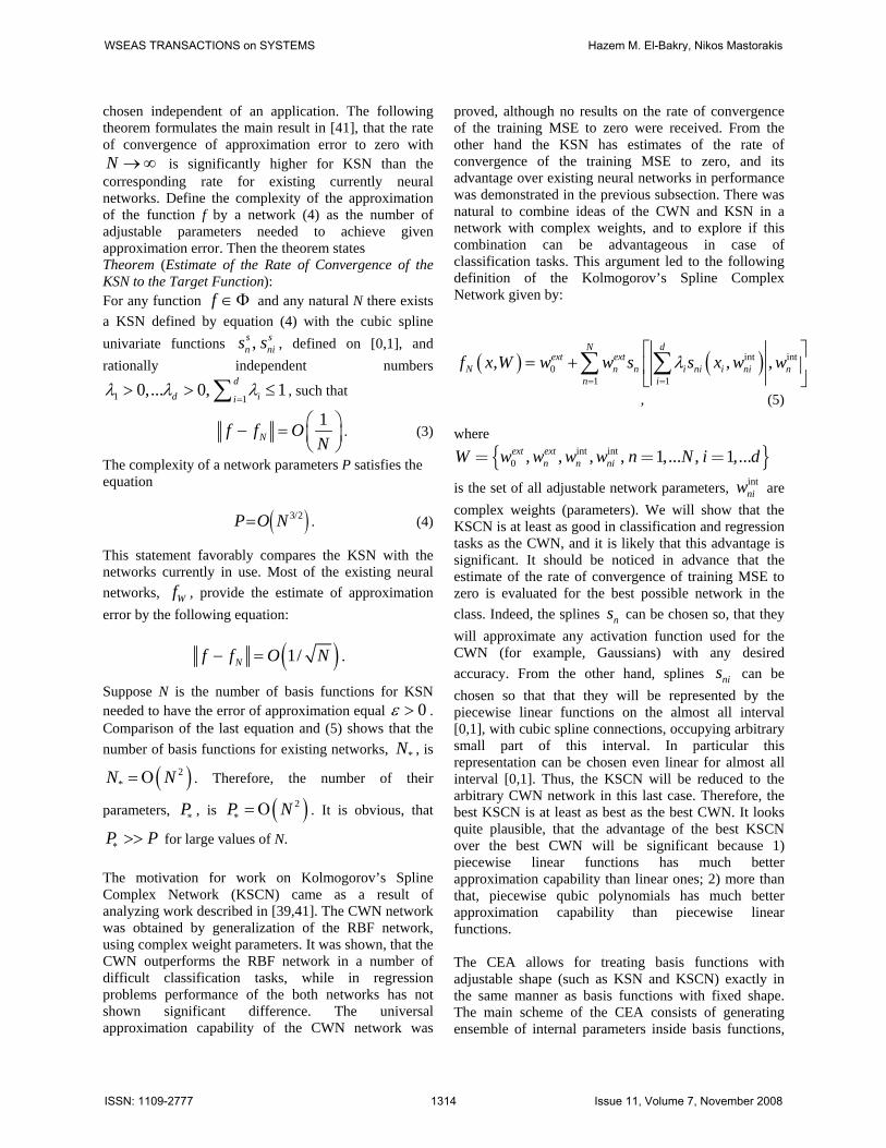
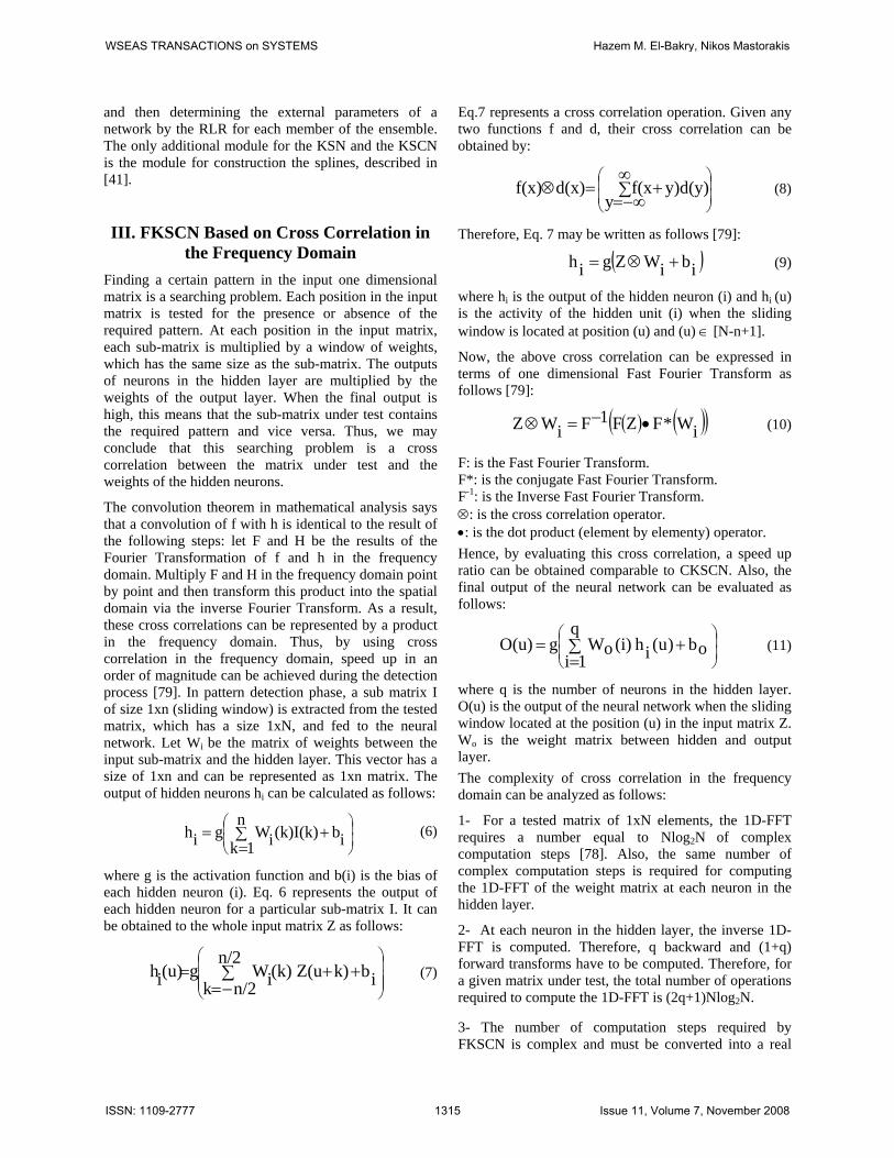
The theoretical speed up ratio for detecting (nxn) real valued submatrix in a large real valued matrix (NxN) using FKSCN is shown in Figures 5, 6, 7. Also, the practical speed up ratio for manipulating matrices of different sizes (NxN) and different sized weight matrices (n) using a 700 MHz processor and MATLAB is shown in Figure 8.

2) In case of complex inputs

A) For a one dimensional input matrix

Multiplication of (n) complex-valued weights by (n) complex inputs requires (6n) real operations. This produces (n) real numbers and (n) imaginary numbers. The addition of these numbers requires (2n-2) real operations. Therefore, the number of computation steps required by CKSCN can be calculated as:

θ=2q(4n-1)(N-n+1) (21)



1)n-1)(N-2q(4n

2 ++++

=η (22)

The theoretical speed up ratio for searching short complex successive (n) data in a long complex-valued input vector (L) using FKSCN is shown in Figures 9, 10, and 11. Also, the practical speed up ratio for manipulating matrices of different sizes (L) and different sized weight matrices (n) using a 700 MHz processor and MATLAB is shown in Figure 12.

B) For a two dimensional input matrix

Multiplication of (n2) complex-valued weights by (n2) real inputs requires (6n2) real operations. This produces (n2) real numbers and (n2) imaginary numbers. The addition of these numbers requires (2n2-2) real operations. Therefore, the number of computation steps required by CKSCN can be calculated as:

θ=2q(4n2-1)(N-n+1)2 (23)


N )n-q(8N )N log1)(5N(2q

1)n-1)(N-2q(4n222

22

22

++++

=η (24)

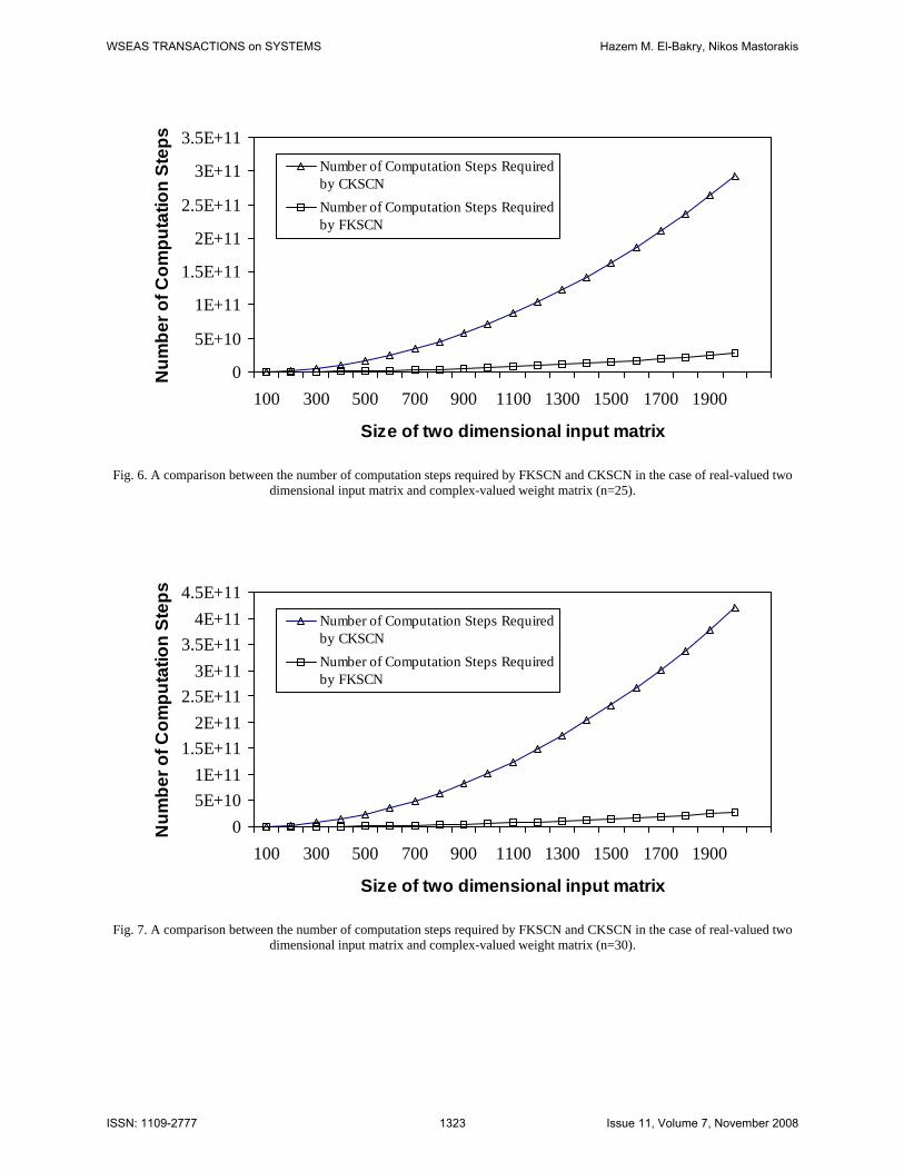
The theoretical speed up ratio for detecting (nxn) complex-valued submatrix in a large complex-valued matrix (NxN) using FKSCN is shown in Figures 13, 14, and 15. Also, the practical speed up ratio for manipulating matrices of different sizes (NxN) and different sized weight matrices (n) using a 700 MHz processor and MATLAB is shown in Figure 16.

In practical implementation, the multiplication process consumes more time than the addition one. The effect of the number of multiplications required for CKSCN in the speed up ratio is more than the number of of multiplication steps required by the FKSCN. Also, the vaiations in Pc clock have an effect on practical computations.

For a one dimensional matrix, from Figures 1,2,3,4,9,10,11, and 12, we can conclude that the response time for vectors with short lengths are faster than those which have longer lengths. For example, the speed up ratio for the vector of length 10000 is faster that of length 1000000. The number of computation steps required for a vector of length 10000 is much less than that required for a vector of length 40000. So, if the vector of length 40000 is divided into 4 shorter vectors of length 10000, the number of computation steps will be less than that required for the vector of length 40000. Therefore, for each application, it is useful at the first to calculate the optimum length of the input vector. The same conclusion can be drawn in case of processing the two dimensional input matrix as shown in Figures 5,6,7,8,13,14,15, and 16. From these Figures, it is clear that the maximum speed up ratio is achieved at image size (N=200) when n=20, then at image size (N=300) when n=25, and at image size (N=400) when n=30. This confirms our previous results presented in [84] on fast subimage detection based on neural networks and image decomposition. Using this technique, it was proved that the speed up ratio of neural networks becomes faster when the input image is divided into many subimages and each subimage is processed in the frequency domain separately using a single fast neural processor. Another point of interest should be noted. In CKSCN, if the whole input data (N) is available, then there is a waiting time for each group of (n) input data so that CKSCN can release their output for the previous group of (n) data. In contrast, FKSCN can process the total N data directly with zero waiting time. For example, if the total (N) input data is appeared at the input neurons, then: 1- CKSCN can process only data of size (n) as the number of input neurons = (n).



2- The first group of (n) data is processed by CKSCN. 3- The second group of (n) data must wait for a waiting time = τ, where τ is the response time consumed by CKSCN for treating each group of (n) input data. 4- The third group of (n) data must wait for a waiting time = 2τ corresponding to the total waiting time required by CKSCN for treating the previous two groups. 5- The fourth (n) data must wait for a waiting time = 3τ. 6- The last group of (n) data must wait for a waiting time = (N-n)τ. As a result, the wasted waiting time in the case of CKSCN is (N-n)τ. In the case of FKSCN, there is no waiting time as the whole input data (Z) of length (N) will be processed directly and the time consumed is the only time required by FKSCN themselves to produce their output.

V. Conclusion A new approach to speed up the operation of Kolmogorov’s Spline Complex Network has been presented. Theoretical computations have shown that FKSCN require fewer computation steps than conventional one. This has been achieved by applying cross correlation in the frequency domain between the input data and the input weights of neural networks. Simulation results have confirmed this proof by using MATLAB. Furthermore, neural network architecture with complex weights and potentially complex inputs, in context of adaptive dynamic modeling of time-variant multidimensional data has been discussed.

References [1] H. Adeli, S-L. Hung, Machine learning. Neural networks,

genetic algorithms, and fuzzy systems, New York, NY: John Wiley & Sons, 1995.

[2] H. Adeli, A. Samant, Wavelets to enhance computational intelligence, In P. Sincak, J. Vascak (Eds). Quo vadis computational intelligence? New trends and approaches in computational intelligence (pp. 399-407). Heidelberg; New York: Physica-Verlag 2000.

[3] I. N. Aizenberg, N. N. Aizenberg, , and V. Joos, Multi-valued and universal binary neurons- Theory, learning, and applications, Boston, MA: Kluwer Academic Publishers, 2000.

[4] A. Albert, Regression and the Moore-Penrose pseudoinverse. New York, NY: Academic Press, 1972.

[5] R. T. Antony, Principles of data fusion automation, Norwood, MA: Artech House, 1995.

[6] P. Arena, L. Fortuna, G. Muscato, and M. G. Xibilia, Neural networks in multidimensional domains, Fundamentals and new trends in modeling and control. New York: Springer, 1998.

[7] K. Astrom, B. Wittenmark, Adaptive control, Reading, MA: Addison-Wesley, 1995.

[8] T. Bäck, Evolutionary algorithms in theory and practice, New York, NY: Oxford University Press, 1996.

[9] A. R. Barron, Universal approximation bounds for superpositions of a sigmoidal function, IEEE Transactions on Information Theory, 39(4), 930-945, 1993.

[10] A. R. Barron, Approximation and estimation bounds for artificial neural networks, Machine Learning, 14(1), 115-133, 1994.

[11] J. Bezdek, On the relationship between neural networks, pattern recognition and intelligence, International Journal on Approximating Reasoning, 6(2), 85-107, 1992.

[12] J. C. Bezdek, J. Keller, Krishnapuram, R., and Pal, N. R., Fuzzy models and algorithms for pattern recognition and image processing. Norwell, MA: Kluwer Academic Publishers, 1999.

[13] C. M. Bishop, Neural networks for pattern recognition, New York, NY: Oxford University Press, 1995.

[14] P. S. Bradley, U. M. Fayyad, Refining initial points for K-means clustering, In 15th International Conference on Machine Learning (pp. 91-99). Los Altos, CA: Morgan Kaufmann, 1998.

[15] Breiman, L., Friedman, J. H., Olshen, R. A, and Stone, C. J., Classification and regression trees, Boca Raton, FL: Chapman & Hall/CRC, 1984.

[16] L. Breiman, Hinging hyperplanes for regression, classification, and function approximation, IEEE Transactions on Information Theory, 39(4), 999-1013, 1993.

[17] L. Breiman, Bagging predictors, Machine Learning, 24(1), 123-140, 1996.

[18] L. Breiman, Combining predictors, In A. Sharkey (Ed.). Combining artificial neural nets: Ensemble and modular multi-net systems (pp. 31-50). London: Springer, 1999.

[19] P. Congdon, Bayesian statistical modeling. Chichester, West Sussex: John Wiley & Sons, Ltd 2006.

[20] N. Cristianini, J. Shawe-Taylor, An introduction to support vector machines, Cambridge, UK: Cambridge University Press, 2000.

[21] R. O. Duda, P. E. Hart, D. G. Stork, Pattern classification, New York, NY: JohnWiley & Sons, Inc., 2001.

[22] G. S. Fishman, Monte Carlo. Concepts, algorithms, and applications, New York, NY: Springer, 1995.

[23] K. Fukunaga, Introduction to statistical pattern recognition, New York, NY: Academic Press, 1990.

[24] G. Georgiou, C. Koutsougeras, Complex domain back-propagation, IEEE Transactions on Circuits and Systems-II: Analog and Digital Signal Processing, 39(5), 330-334, 1992.

[25] F. Girosi, T. Poggio, Representation properties of networks: Kolmogorov’s theorem is irrelevant, Neural Computation, 1(4), 465-469, 1989.

[26] J. C. Goswami, A. K. Chan, Fundamentals of wavelets. Theory, algorithms, and applications. New York, NY: John Wiley & Sons, Inc, 1999.

[27] J. Hawkins, S. Blakeslee, On intelligence, New York: Henry Holt and Company, 2004.

[28] S. Haykin, Adaptive filter theory. Fourth edition, Upper Saddle River, NJ: Prentice Hall, 2002.

[29] S. Haykin, Neural networks, a comprehensive foundation, New York, NY: IEEE Press, 1994.

[30] S. Haykin, (Ed.), Kalman filtering and neural networks, New York, NY: John Wiley & Sons, 2001.

[31] R. Hecht-Nielsen, Kolmogorov’s mapping neural network existence theorem, In IEEE International Conference on



Neural Networks, 3 (pp. 11-13). New York, NY: IEEE Press, 1987.

[32] A. Hirose, (Ed.). Complex-valued neural networks, Singapore: World Scientific Publishers, 2003.

[33] A. Hirose, Complex-valued neural networks, Berlin: Springer, 2006.

[34] S. A. Hovanessian, Introduction to sensor systems, Norwood, MA: Artech House, 1984.

[35] B. Igelnik, and Y. - H Pao, Stochastic choice of basis functions in adaptive function approximation and the functional-link net, IEEE Transactions on Neural Networks, 6(6), 1320-1329, 1995.

[36] B. Igelnik, Y- H Pao, and S. R. LeClair, An approach for optimization of a continuous function with many local minima, In 30th Annual Conference on Information Sciences and Systems, 2 (pp. 912-917), Department of Electrical Engineering, Princeton University, Princeton, NJ, 1996.

[37] B. Igelnik, , Y- H Pao., S. R. LeClair, & C. Y.Shen, The ensemble approach to neural network learning and generalization, IEEE Transactions on Neural Networks, 10(1), 19-30, 1999.

[38] B. Igelnik, Some new adaptive architectures for learning, generalization, and visualization of multivariate data, In P. Sincak and J. Vascak (Eds.). Quo Vadis Computational Intelligence? New Trends and Approaches in Computational Intelligence (pp. 63-78). Heidelberg; New York, NY: Physica-Verlag, 2000.

[39] B. Igelnik, M. Tabib-Azar, & S. LeClair, A net with complex weights, IEEE Transactions on Neural Networks, 12(2), 236-249, 2001a.

[40] B. Igelnik, Method for visualization of multivariate data in a lower dimension, In SPIE Visual Data Exploration and Analysis VIII, 4302, (pp. 168-179), San Jose, CA, 2001b.

[41] B. Igelnik, N. Parikh, Kolmogorov’s spline network, IEEE Transactions on Neural Networks, 14(3), 725-733, (2003a).

[42] B. Igelnik, Visualization of large multidimensional datasets in a lower dimension, SBIR Phase I Final Report, #0232775, NSF. 2003b.

[43] B. Igelnik, Visualization of large multidimensional datasets in a lower dimension. SBIR Phase II Proposal, #0349713, NSF, 2003c.

[44] B. Igelnik, N. Parikh, System for multidimensional data modeling, optimization, analysis and visualization, Submitted to US PTO, 2004.

[45] B. Igelnik, Neural network model with clustering ensemble approach, Submitted to US PTO, 2005.

[46] B. Igelnik, Visual tools for large datasets with applications, SBIR Phase I Proposal, #0637258, NSF, 2006.

[47] P. Jackson, Introduction to expert systems, Reading, MA: Addison-Wesley, 1986.

[48] M. Kalos, P. A. Witlock, Monte Carlo methods, New York, NY: John Wiley & Sons, 1986.

[49] M. S. Kim, C. C. Guest, Modification of back-propagation for complex-valued signal processing in frequency domain, In International Joint Conference on Neural Networks 1990 San Diego (pp. 27-31). New York: IEEE, 1990.

[50] V. Kurková, Kolmogorov's theorem is relevant, Neural Computation, 3(4), 617-622, 1991.

[51] V. Kurková, Kolmogorov’s theorem and multilayer neural networks, Neural Networks, 5(3), 501-506, 1992.

[52] A. N. Kolmogorov, On the representation of continuous functions of many variables by superposition of continuous functions of one variable and addition. Doklady Akademii Nauk SSSR, 114(5), 953-956. (1963). Translations American Mathematical Society, 2(28), 55-59, 1957.

[53] H. Leung, S. Haykin, The complex backpropagation algorithm, IEEE Transactions on Signal Processing, 39(9), 2101-2104, 1991.

[54] G. Li, K. B. Yu, Modeling and simulation of coherent Weibull clutter. IEE Proceedings, Part. F, 136(1), 1-9, 1988.

[55] L. Ljung, System identification theory for the user. Englewood Cliffs, NJ: Prentice Hall, 2000.

[56] G. G. Lorentz, G. G. von Golitschek, M. Y. Makovoz, Constructive approximation, Advanced problems. New York: Springer, 1996.

[57] F-L. Luo, R. Unbehauen, Applied neural networks for signal processing. NY: Cambridge University Press, 1997.

[58] H. Mhascar, C. Miccheli, Approximation by superposition of sigmoidal and radial basis functions, Advances in Applied Mathematics, 13(3), 350-373, 1992.

[59] M. Mitchell, An introduction to genetic algorithms, Cambridge, MA: The MIT Press, 1996.

[60] H. Niederreiter, Quasi-Monte Carlo methods and pseudorandom numbers. Bulletin of American Mathematical Society, 84, 957-1041, 1978.

[61] N. J. Nilsson, Artificial intelligence, A new synthesis. SanFrancisco, CA: Morgan Kaufmann Publishers, 1998.

[62] N. Nitta, An extension of the backpropagation algorithm to complex numbers, Neural Networks, 10(8), 1391-1415, 1997.

[63] N. Nitta, On the inherent property of the decision boundary in complex-valued neural networks, Neurocomputing, 50(1), 291-303, 2003.

[64] A. V. Oppenheim, R. W. Schafer, Digital signal processing, Englewood Cliffs, NJ: Prentice Hall, 1975.

[65] W. Pedricz Computational intelligence, An introduction. Boca Raton, FL: CRC Press, 1998.

[66] P. M. Prenter, Splines and variational methods, New York, NY: John Wiley & Sons, 1975.

[67] A. W. Rihaczek, S. J. Hershkowitz, Radar resolution and complex-image analysis, Norwood, MA: Artech House, 1996.

[68] M. I. Scolnik, (Ed.), Radar handbook, Second edition. New York, NY: McGraw-Hill, 1990.

[69] A. B. Shidlovskii, Transcendental numbers, Berlin: Walter de Gruyter, 1989.

[70] D. A. Sprecher, On the structure of continuous functions of several variables, Transactions of American Mathematical Society, 115(3), 340-355, 1965.

[71] D. A. Sprecher, A numerical implementation of Kolmogorov’s superpositions, Neural Networks, 9(5), 765-772, 1996.

[72] D. A. Sprecher, A numerical implementation of Kolmogorov’s superpositions II, Neural Networks, 10(3), 447-457, 1997.

[73] M. Stone, Cross-validatory choice and assessment of statistical predictions. Journal of the Royal Statistical Society, B 36(1), 11-147, 1974.

[74] L. D. Stone, C. A. Barlow, and T. L. Corwin, Bayesian multiple target tracking. Boston, MA: Artech House, 1999.



[75] A. H. Stroud, Approximate calculation of multiple integrals, Englewood Cliffs, NJ: Prentice-Hall, 1971.

[76] A. D. Zapranis, A. – P. Refenes, Principles of neural model identification, selection and adequacy, London: Springer, 1999.

[77] J. Zurada, R. Marks, and C. Robinson, (Eds.). Introduction to computational intelligence: Imitating life. Piscataway, NJ: IEEE Press, 1994.

[78] J. W. Cooley, and J. W. Tukey, An algorithm for the machine calculation of complex Fourier series, Math. Comput. 19, 297–301 1965.

[79] Hazem M. El-Bakry, New Faster Normalized Neural Networks for Sub-Matrix Detection using Cross Correlation in the Frequency Domain and Matrix Decomposition, Applied Soft Computing journal, vol. 8, issue 2, 1131-1149, March 2008.

[80] S. Jankowski, A. Lozowski, and M. Zurada, Complex-valued Multistate Neural Associative Memory, IEEE Trans. on Neural Networks, vol.7, 1491-1496, 1996.

[81] Hazem M. El-Bakry, Nikos Mastorakis, New Fast Normalized Neural Networks for Pattern Detection, Image and Vision Computing Journal, 25(11), 1767-1784, 2007.

[82] H. M. El-Bakry, Q. Zhao, Fast Object/Face Detection Using Neural Networks and Fast Fourier Transform, International Journal of Signal Processing, 1(3), 182-187, 2004.

[83] H. M. El-Bakry, Q. Zhao, Fast Pattern Detection Using Normalized Neural Networks and Cross Correlation in the

Frequency Domain, EURASIP Journal on Applied Signal Processing, Special Issue on Advances in Intelligent Vision Systems: Methods and Applications—Part I, vol. 2005, No. 13, 2054-2060, August 2005.

[84] H. M. El-Bakry, Face detection using fast neural networks and image decomposition, Neurocomputing Journal, vol. 48, 1039-1046, 2002.

[85] H. M. El-Bakry, Human Iris Detection Using Fast Cooperative Modular Neural Nets and Image Decomposition, Machine Graphics & Vision Journal (MG&V), 11(4), 498-512, 2002.

[86] H. M. El-Bakry, Automatic Human Face Recognition Using Modular Neural Networks, Machine Graphics & Vision Journal (MG&V), 10(1), 47-73, 2001.

[87] Hazem M. El-Bakry, New Fast Time Delay Neural Networks Using Cross Correlation Performed in the Frequency Domain, Neurocomputing Journal, vol. 69, 2360-2363, October 2006.

[88] Hazem M. El-Bakry and Mohamed Hamada, A New Implementation for High Speed Neural Networks in Frequency Space, Lecture Notes in Computer Science, Springer, KES 2008, Part I, LNAI 5177, 33-40, 2008.

0

5E+10

1E+11

1.5E+11

2E+11

2.5E+11

10000 2E+05 5E+05 1E+06 2E+06 3E+06 4E+06

Length of one dimensional input matrix

Num

ber o

f Com

puta

tion

Step

s

Number of Computation Steps Requiredby CKSCN

Number of Computation Steps Requiredby FKSCN

Fig. 1. A comparison between the number of computation steps required by FKSCN and CKSCN in case of real-valued one

dimensional input matrix and complex-valued weight matrix (n=400).



0

5E+10

1E+11

1.5E+11

2E+11

2.5E+11

3E+11

3.5E+11

10000 2E+05 5E+05 1E+06 2E+06 3E+06 4E+06


Num

ber o

f Com

puta

tion

Step

sNumber of Computation Steps Requiredby CKSCN


Fig. 2. A comparison between the number of computation steps required by FKSCN and CKSCN in the case of real-valued one


0

1E+11

2E+11

3E+11

4E+11

5E+11

10000 2E+05 5E+05 1E+06 2E+06 3E+06 4E+06


Num

ber o

f Com

puta

tion

Step

s



Fig. 3. A comparison between the number of computation steps required by FKSCN and CKSCN in the case of real-valued one




0

5

10

15

20

25

30

35

40

10000 2E+05 5E+05 1E+06 2E+06 3E+06 4E+06


Spee

d up

Rat

io

Practical Speed up ratio (n=400)Practical Speed up ratio (n=625)Practical Speed up ratio (n=900)

Fig. 4. Practical speed up ratio for Kolmogorov’s Spline Complex Network in case of one dimensional real-valued input matrix

and complex-valued weights.

0

2E+10

4E+10

6E+10

8E+10

1E+11

1E+11

1E+11

2E+11

2E+11

2E+11

100 300 500 700 900 1100 1300 1500 1700 1900

Size of two dimensional input matrix

Num

ber o

f Com

puta

tion

Step

s



Fig. 5. A comparison between the number of computation steps required by FKSCN and CKSCN in the case of real-valued two




0

5E+10

1E+11

1.5E+11

2E+11

2.5E+11

3E+11

3.5E+11

100 300 500 700 900 1100 1300 1500 1700 1900


Num

ber o

f Com

puta

tion

Step





0

5E+10

1E+11

1.5E+11

2E+11

2.5E+11

3E+11

3.5E+11

4E+11

4.5E+11

100 300 500 700 900 1100 1300 1500 1700 1900


Num

ber o

f Com

puta

tion

Step

s







0

5

10

15

20

25

30

35

40

100 300 500 700 900 1100 1300 1500 1700 1900


Spee

d up

Rat

io

Speed up Ratio (n=20)Speed up Ratio (n=25)Speed up Ratio (n=30)

Fig. 8. Practical speed up ratio for Kolmogorov’s Spline Complex Network in case of two dimensional real-valued input matrix

and complex-valued weights.

0

5E+10

1E+11

1.5E+11

2E+11

2.5E+11

3E+11

3.5E+11

4E+11

4.5E+11

10000 2E+05 5E+05 1E+06 2E+06 3E+06 4E+06


Num

ber o

f Com

puta

tion

Step

s



Fig. 9. A comparison between the number of computation steps required by FKSCN and CKSCN in the case of complex-valued

one dimensional input matrix and complex-valued weight matrix (n=400).



0.00E+00

1.00E+11

2.00E+11

3.00E+11

4.00E+11

5.00E+11

6.00E+11

7.00E+11

10000 2E+05 5E+05 1E+06 2E+06 3E+06 4E+06


Num

ber o

f Com

puta

tion

Step





0.00E+001.00E+112.00E+113.00E+114.00E+115.00E+116.00E+117.00E+118.00E+119.00E+111.00E+12

10000 2E+05 5E+05 1E+06 2E+06 3E+06 4E+06


Num

ber o

f Com

puta

tion

Step

s







0

10

20

30

40

50

60

70

80

10000 2E+05 5E+05 1E+06 2E+06 3E+06 4E+06


Spee

d up

Rat

io

Practical Speed up ratio (n=400)Practical Speed up ratio (n=625)Practical Speed up ratio (n=900)

Fig. 12. Practical speed up ratio for Kolmogorov’s Spline Complex Network in case of one dimensional complex-valued input

matrix and complex-valued weights.

0

5E+10

1E+11

2E+11

2E+11

3E+11

3E+11

4E+11

4E+11

100 300 500 700 900 1100 1300 1500 1700 1900


Num

ber

of C

ompu

tatio

n St

eps




two dimensional input matrix and complex-valued weight matrix (n=20).



0

1E+11

2E+11

3E+11

4E+11

5E+11

6E+11

7E+11

100 300 500 700 900 1100 1300 1500 1700 1900


Num

ber o

f Com

puta

tion

Step





0.00E+00

1.00E+11

2.00E+11

3.00E+11

4.00E+11

5.00E+11

6.00E+11

7.00E+11

8.00E+11

9.00E+11

100 300 500 700 900 1100 1300 1500 1700 1900


Num

ber o

f Com

puta

tion

Step

s







0

10

20

30

40

50

60

70

100 300 500 700 900 1100 1300 1500 1700 1900


Spee

d up

Rat

io

Speed up Ratio (n=20)Speed up Ratio (n=25)Speed up Ratio (n=30)

Fig. 16. Practical speed up ratio for Kolmogorov’s Spline Complex Network in case of two dimensional complex-valued input

matrix in and complex-valued weights.



A Novel Fast Kolmogorov's Spline Complex Network for ... · A Novel Fast Kolmogorov's Spline...

Documents

Transcript of A Novel Fast Kolmogorov's Spline Complex Network for ... · A Novel Fast Kolmogorov's Spline...