
A NOVEL APPROACH FOR SIMULATING SOIL AND PIPE …
239
A NOVEL APPROACH FOR SIMULATING SOIL AND PIPE RESPONSE TO SEASONAL, ENVIRONMENTAL AND FIELD CONDITIONS A Thesis Submitted to the Faculty of Graduate Studies and Research In Partial Fulfillment of the Requirements For the Degree of Doctor of Philosophy in Environmental Systems Engineering University of Regina By Ramy M. Saadeldin Regina, Saskatchewan April 2016 Copyright 2016: R. Saadeldin
Transcript of A NOVEL APPROACH FOR SIMULATING SOIL AND PIPE …

A NOVEL APPROACH FOR SIMULATING SOIL AND PIPE RESPONSE TO
SEASONAL, ENVIRONMENTAL AND FIELD CONDITIONS
A Thesis
Submitted to the Faculty of Graduate Studies and Research
In Partial Fulfillment of the Requirements
For the Degree of
Doctor of Philosophy
in
Environmental Systems Engineering
University of Regina
By
Ramy M. Saadeldin
Regina, Saskatchewan
April 2016
Copyright 2016: R. Saadeldin

UNIVERSITY OF REGINA
FACULTY OF GRADUATE STUDIES AND RESEARCH
SUPERVISORY AND EXAMINING COMMITTEE
Ramy M. Saadeldin, candidate for the degree of Doctor of Philosophy in Environmental Systems Engineering, has presented a thesis titled, A Novel Approach for Simulating Soil and Pipe Response to Seasonal, Environmental and Field Conditions, in an oral examination held on April 12, 2016. The following committee members have found the thesis acceptable in form and content, and that the candidate demonstrated satisfactory knowledge of the subject material. External Examiner: *Dr. Mohammed Sakr, Machibroda Engineering
Supervisor: Dr. Amr Henni, Industrial Systems Engineering
Committee Member: **Dr. Yee-Chung Jin, Environmental Systems Engineering
Committee Member: Dr. Ezeddin Shirif, Petroleum Systems Engineering
Committee Member: Dr. Osman Salad Hersi, Department of Geology
Chair of Defense: Dr. Mark Brigham, Department of Biology *Via Skype **Not present at defense

i
ABSTRACT
Climate change related problems are increasing in occurrence and severity leading
to significant economic losses in many places of the world. In semi-arid environments,
like Saskatchewan, the main phenomenon involved in pipe breakages is the volume
change behavior of unsaturated clay deposits. Underground pipelines are typically
buried within the upper zone of soil deposits, and therefore, are highly affected by soil
nature and the different environmental conditions present on the ground surface. To
accurately model field conditions, a mathematical formulation of native soil conditions
was developed based on laboratory and field test results. Volume-mass constitutive
surfaces were established based on a bimodal soil water characteristic curve (SWCC)
and other constitutive relationships.
In order to simulate the response of soil and pipe to various meteorological
conditions, a numerical framework was developed and validated. The strength of the
developed numerical framework lays in the use of bimodal SWCC and modeling the
hydraulic characteristics of a cracked soil structure. This research study also utilized, as
a database, the results of a field instrumentation program conducted in the City of
Regina. A hydro-mechanical analysis was implemented to model the volume change
due to variations in mechanical loading conditions and moisture content. Modeling
scenarios were also studied based on variations in pipe diameter, pipe depth and soil
elasticity.
The developed numerical framework provided insight into the sensitivity of pipe
deformation to possible changes in input parameters of the soil-pipe system. The model
was able to capture the transient water flow through saturated-unsaturated soils. The
results of the modeling of weather conditions applied on the soil-pipe system were in
agreement with the field measurements. Specific relationships between the soil-pipe

ii
interaction and seasonal changes in the local meteorological conditions were
established. The model was also used to provide some insight into the real flux
transferred through the pavement structure to the backfill material surrounding the pipe.
Finally, soil and pipe reactions (i.e. soil and pipe displacements, soil volumetric water
content and soil temperature) to applied surface boundary conditions were predicted
based on the validated numerical approach.

iii
ACKNOWLEDGEMENTS
I would like to express my sincere appreciation to my supervisor, Dr. Amr Henni,
for his precious support and continuous encouragement throughout the course of this
research program. I would like to thank, Dr. Yafei Hu, for his overall guidance and critical
appraisal. I would also like to extend my acknowledgement to my advisory committee
members for their valuable suggestions and input.
The financial support provided by the Faculty of Graduate Studies and Research
(FGSR) at the University of Regina, and the City of Regina (Henry Baker Scholarship
Program) is gratefully acknowledged. In addition, I would like to acknowledge the
contribution of the National Research Council Centre for Sustainable Infrastructure
Research for allowing access to their research facilities.
Many thanks, to my colleagues and staff at the Faculty of Engineering and Applied
Science, for making my stay at the University of Regina an unforgettable one. I would
also like to thank Mr. Gene Froc who gave me invaluable support that helped me to
reach this point.
Last but not the least, I am extremely grateful to my parents, wife, sister and
brothers for their continuous support, and to my children for providing me with the
motivation to complete my thesis.

iv
TABLE OF CONTENTS
ABSTRACT..................................................................................................................... I
ACKNOWLEDGEMENTS ..............................................................................................III
TABLE OF CONTENTS ................................................................................................ IV
LIST OF FIGURES ....................................................................................................... VII
LIST OF TABLES ........................................................................................................ XII
CHAPTER 1: INTRODUCTION ...................................................................................... 1
1.1 Definitions ................................................................................................................. 1
1.2 Problem Recognition ................................................................................................ 5
1.3 Engineering Significance .......................................................................................... 6
1.4 Research Objectives ................................................................................................ 8
1.5 Finite Element Approach .......................................................................................... 9
1.6 Contributions ...........................................................................................................13
1.7 Outline of this Research ..........................................................................................15
CHAPTER 2: LITERATURE REVIEW...........................................................................17
2.1 Surficial Geology .....................................................................................................17
2.2 Climate Conditions ..................................................................................................19
2.3 Expansive Soils .......................................................................................................22
2.4 Clay Mineralogy .......................................................................................................25
2.5 Unsaturated Soil Parameters ...................................................................................30
2.5.1 Stress State Variables .......................................................................................30 2.5.2 Soil Suction .......................................................................................................34
2.6 Desiccation Cracks ..................................................................................................36
2.7 Hydraulic Conductivity Function ...............................................................................41
2.8 Soil Water Characteristic Curve (SWCC) .................................................................42
2.9 Measurements of Soil Moisture-suction Characteristics ...........................................45
2.9.1 Foreword ...........................................................................................................45 2.9.2 Soil Moisture Monitoring (Principle and Techniques) .........................................45 2.9.3 Soil Suction Monitoring (Principle and Techniques) ...........................................47
2.10 Unsaturated Soil-atmosphere Interaction ...............................................................51
2.10.1 Foreword .........................................................................................................51 2.10.2 Soil Evaportranspiration ..................................................................................51 2.10.3 Water Flow ......................................................................................................52 2.10.4 Heat Flow ........................................................................................................55
2.11 Unsaturated Soil-structure Interaction ....................................................................56
2.11.1 Numerical Approaches ....................................................................................56 2.11.2 Volume-mass Constitutive Relationships ........................................................57
2.12 Pipelines Infrastructure ..........................................................................................63
2.13 Applied Loads on Buried Pipes ..............................................................................64
2.13.1 Foreword .........................................................................................................64

v
2.13.2 Soil Load .........................................................................................................65 2.13.3 Live Loads.......................................................................................................67
2.14 Pipe Stresses ........................................................................................................68
2.15 Pipe Deformations .................................................................................................70
2.15.1 Horizontal Deformation....................................................................................70 2.15.2 Bending Displacement ....................................................................................71
2.16 Buried Pipe Damages ............................................................................................73
2.16.1 Failure Mechanisms Associated with Soil Movements.....................................73 2.16.2 Case Studies ...................................................................................................75
2.17 Related Numerical Modeling Studies in the Literature ............................................76
CHAPTER 3: FIELD INVESTIGATION .........................................................................80
3.1 General ...................................................................................................................80
3.2 Field Program Details ..............................................................................................81
3.3 Instrumentation Details ............................................................................................84
3.4 Climate Data ............................................................................................................86
3.5 Backfill and Bedding Soils .......................................................................................90
3.6 Soil Profile and Properties at the Field Site ..............................................................92
3.7 Unsaturated Soil Characteristics ..............................................................................98
3.8 Soil Moisture Field Data ......................................................................................... 102
3.9 Air and Soil Temperatures ..................................................................................... 104
3.10 Measured Pipe Displacements ............................................................................ 104
CHAPTER 4: LOAD-DEFORMATION ANALYSIS UNDER DIFFERENT SOIL AND PIPE CONDITIONS ..................................................................................................... 107
4.1 Problem Statement ................................................................................................ 107
4.2 Governing Equations ............................................................................................. 107
4.3 Modeling Overview, Geometry and Boundary Conditions ...................................... 109
4.4 Numerical Modeling versus Analytical Results ....................................................... 113
4.5 Pipe Deformations ................................................................................................. 115
CHAPTER 5: PIPE RESPONSE TO RELATIVE SATURATION OF SURROUNDING SOIL ............................................................................................................................ 120
5.1 Problem Statement ................................................................................................ 120
5.2 Governing Equations ............................................................................................. 120
5.3 Modeling Overview, Geometry and Boundary Conditions ...................................... 122
5.4 Numerical Modeling versus Analytical Results ....................................................... 127
5.5 Soil Saturation - Pipe Displacement Analysis ........................................................ 127
CHAPTER 6: MATHEMATICAL FORMULATIONS OF SOIL-WATER INTERACTION UNDER UNSATURATED SOIL CONDITIONS ........................................................... 134
6.1 Problem Statement ................................................................................................ 134
6.2 Methodology .......................................................................................................... 135
6.3 Fracture Depth Formulation ................................................................................... 135
6.4 Hydraulic Conductivity Formulation ........................................................................ 142

vi
6.5 Development of a Bimodal SWCC ......................................................................... 143
6.6 Volume-mass Constitutive Relationships ............................................................... 148
6.7 Water Flow Mathematical Formulation ................................................................... 157
6.8 Parametric Study ................................................................................................... 157
6.8.1 General ........................................................................................................... 157 6.8.2 Methodology ................................................................................................... 158 6.8.3 Results and Discussion ................................................................................... 160
CHAPTER 7: SOIL-PIPE-ATMOSPHERE INTERACTION UNDER FIELD CONDITIONS .............................................................................................................. 168
7.1 Problem Statement ................................................................................................ 168
7.2 Methodology .......................................................................................................... 168
7.3 Geometry and Boundary Conditions ...................................................................... 170
7.4 Mathematical Formulation ..................................................................................... 174
7.4.1 Evapotranspiration Process ............................................................................ 174 7.4.2 Water Flow Equations ..................................................................................... 175 7.4.3 Stress-strain Equations ................................................................................... 176
7.5 Climate Data .......................................................................................................... 177
7.6 Pavement Boundary Conditions ............................................................................ 178
7.7 Soil Temperature Analysis Results ........................................................................ 178
7.8 Soil Moisture Analysis Results ............................................................................... 182
7.9 Soil and Pipe Displacements with Time ................................................................. 187
CHAPTER 8: SUMMARY, CONCLUSION AND FUTURE WORK .............................. 189
8.1 Engineering Significance and Applications ............................................................ 189
8.2 Summary of Results .............................................................................................. 189
8.2.1 Field Investigation ........................................................................................... 189 8.2.2 Load-deformation Analysis .............................................................................. 190 8.2.3 Pipe Response to Unsaturated Soil Conditions ............................................... 191 8.2.4 Soil-water Interaction in Highly Plastic Clays ................................................... 192 8.2.5 Soil-pipe-atmosphere Interaction under Field Conditions ................................ 194
8.3 Conclusion ............................................................................................................. 196
8.4 Future Work ........................................................................................................... 197
REFERENCES ............................................................................................................ 198
APPENDIX .................................................................................................................. 208

vii
LIST OF FIGURES
Figure 1.1: Research concepts ....................................................................................... 3
Figure 1.2: Conceptual presentation of key research elements ...................................... 4
Figure 1.3: Summary of the field investigation and numerical modeling programs .........14
Figure 2.1: A 100-year average precipitation for the City of Regina (Environment
Canada) ........................................................................................................................21
Figure 2.2: A 100-year average temperature for the City of Regina (Environment
Canada) ........................................................................................................................21
Figure 2.3: A general presentation of soil mechanics principles showing the role of the
surface flux boundary condition after (Ng and Menzies, 2007) ......................................24
Figure 2.4: The relationship between soil plasticity and swelling potential, after (Van Der
Merwe, 1964) ................................................................................................................29
Figure 2.5: A theoretical model for cracking mechanical mechanism after (Anderson,
2005) .............................................................................................................................40
Figure 2.6: Typical soil water characteristic curve of clay soil ........................................44
Figure 2.7: Measurement methods of soil-water characteristics ....................................48
Figure 2.8: The unsaturated soil stress state parameters using the combination of (σ –
ua), and matric suction (ua – uw) (Fredlund and Vanapalli, 2002)....................................62
Figure 2.9: Constitutive surfaces for an unsaturated, swelling soil .................................62
Figure 2.10: Principle stresses of a pipeline (Ng, 1994) .................................................69
Figure 2.11: Stresses in a pipeline under longitudinal extension (Ng, 1994) ..................69
Figure 2.12: Stresses in a pipeline under longitudinal bending conditions (Ng, 1994) ....69
Figure 2.13: Pipe deformation diagram (Ring Theory) ...................................................72
Figure 2.14: Pipe displacement due to axial bending .....................................................72
Figure 2.15: Common soil movement induced failure modes for pipe networks after
(Cassa, 2008) ................................................................................................................74
Figure 3.1: Site location and layout ................................................................................82
Figure 3.2: Summary of field instrumentation types .......................................................82

viii
Figure 3.3: Schematic of the installed sensors layout at the field site ............................85
Figure 3.4: Daily and cumulative precipitation at the field site ........................................87
Figure 3.5: Daily air temperature at the field site ............................................................87
Figure 3.6: Daily wind speed at the field site ..................................................................88
Figure 3.7: Daily net radiation at the field site ................................................................88
Figure 3.8: Daily relative humidity at the field site ..........................................................89
Figure 3.9: Grain size distribution for backfill materials (sand and mixed concrete) .......91
Figure 3.10: Water content and dry unit weight profiles with depth at the field site ........94
Figure 3.11: Grain size distribution of Regina clay and clay till ......................................95
Figure 3.12: Soil water characteristic curve (SWCC) for Regina Clay ............................99
Figure 3.13: Soil water characteristic curve (SWCC) for clay till.....................................99
Figure 3.14: Soil water characteristic curves (SWCCs) for the backfill materials .......... 100
Figure 3.15: Hydraulic conductivity functions for Regina clay and clay till .................... 100
Figure 3.16: Hydraulic conductivity functions for the backfill materials ......................... 101
Figure 3.17: Volumetric water content in the clay deposit at various levels .................. 103
Figure 3.18: Estimated soil suction in the clay deposit at various levels ....................... 103
Figure 3.19: Air and soil temperature observed at the field site ................................... 105
Figure 3.20: Pipe displacements and soil pressures at the field site ............................ 106
Figure 3.21: Pipe displacements at the field site .......................................................... 106
Figure 4.1: Summary of soil-pipe interaction model for parametric study analysis ....... 110
Figure 4.2: Model geometry and definition of the problem ........................................... 110
Figure 4.3: Generated mesh ........................................................................................ 111
Figure 4.4: Effect of the trench width on the maximum pipe deformations ................... 114
Figure 4.5: Effect of soil modulus of elasticity on the overall soil surface displacement116
Figure 4.6: Effect of soil cover height and loading conditions on pipe deformation ...... 116

ix
Figure 4.7: Effect of the backfill modulus of elasticity on pipe deformations ................. 119
Figure 4.8: Effect of the soil cover thickness and loading conditions on pipe deformations
.................................................................................................................................... 119
Figure 5.1: Schematic diagram of the effect of dry and wet soil conditions on the pipe
performance after (Rajeev et al., 2012) ....................................................................... 124
Figure 5.2: Summary of the modeling procedure for displacement analysis ................ 124
Figure 5.3: Geometry for the two-dimensional soil-pipeline model ............................... 125
Figure 5.4: Theoretical model for the analysis of a buried pipe under unsaturated soil
conditions .................................................................................................................... 125
Figure 5.5: Influence of the pipe burial depth on the pipe displacements ..................... 130
Figure 5.6: Maximum displacements versus normalized volumetric water content ...... 130
Figure 5.7: Pipe displacements due to the variation in soil moisture content under hinged
end restraints ............................................................................................................... 131
Figure 5.8: Pipe displacements due to the variation in the soil moisture content under
fixed end restraints ...................................................................................................... 131
Figure 5.9: Pipe displacements in case of both hinged and fixed end restraints for a low
elastic modulus magnitude (i.e. PVC pipe) .................................................................. 133
Figure 5.10: Pipe displacements in case of hinged and fixed end restraints for a high
elastic modulus magnitude (i.e. steel pipe) .................................................................. 133
Figure 6.1: A typical desiccated soil profile and idealized matric suction profile, after
(Lau, 1987) .................................................................................................................. 138
Figure 6.2: Estimated cracking depth at different ground water depths (linear elastic
theory) ......................................................................................................................... 140
Figure 6.3: Estimated cracking depth at a ground water depth of 9.5m (shear strength
approach) .................................................................................................................... 140
Figure 6.4: Estimated cracking depth at a ground water depth of 16 m (shear strength
approach) .................................................................................................................... 141
Figure 6.5: Bimodal SWCC and laboratory suction measurements .............................. 146
Figure 6.6: SWCC shapes at different values for the fitting parameter (a) ................... 146
Figure 6.7: SWCC shapes at different values for the fitting parameter (b) ................... 147
Figure 6.8: Normalized volumetric water content versus mean normal stress .............. 151

x
Figure 6.9: Parametric analysis for normalized volumetric water content versus mean
normal stress relationship ............................................................................................ 152
Figure 6.10: Degree of saturation versus volumetric water content .............................. 153
Figure 6.11: Parametric analysis for degree of saturation versus volumetric water
content relationship ..................................................................................................... 154
Figure 6.12: Volumetric water content constitutive surfaces ........................................ 155
Figure 6.13: Void ratio constitutive surfaces ................................................................ 155
Figure 6.14: Degree of saturation constitutive surfaces ............................................... 156
Figure 6.15: Soil column configuration for the parametric study ................................... 159
Figure 6.16: Predicted suction profiles for Bimodal SWCC versus Unimodal SWCC .. 161
Figure 6.17: Predicted volumetric water content profiles for Bimodal SWCC versus
Unimodal SWCC ......................................................................................................... 161
Figure 6.18: Hydraulic conductivity factor versus elapsed time .................................... 162
Figure 6.19: Hydraulic conductivity versus elapsed time .............................................. 162
Figure 6.20: Predicted suction versus elapsed time at cracking factor magnitudes ..... 164
Figure 6.21: Predicted volumetric water content versus elapsed time at different
cracking depths ........................................................................................................... 164
Figure 6.22: Predicted suction versus elapsed time at different depths....................... 166
Figure 6.23: Predicted volumetric water content versus elapsed time at different depths
.................................................................................................................................... 166
Figure 6.24: Predicted volumetric water content versus elapsed time at different net
surface flux magnitudes ............................................................................................... 167
Figure 6.25: Predicted suction versus elapsed time at different net surface flux
magnitudes .................................................................................................................. 167
Figure 7.1: Soil-pipe-atmosphere modeling processes ................................................ 171
Figure 7.2: Schematic diagram showing the field site conditions ................................. 171
Figure 7.3: The developed mesh for the modeling analysis ......................................... 172
Figure 7.4: Soil temperature versus time in the pipe trench ........................................ 180
Figure 7.5: Soil temperature versus time at a depth of 2.92 m in the pipe trench ........ 180

xi
Figure 7.6: VWC and suction profiles at various levels for the native clay ................... 184
Figure 7.7: VWC at a depth of 0.45 m versus time for the native clay ......................... 184
Figure 7.8: Volumetric water content change in the pipe trench .................................. 186
Figure 7.9: Volumetric water content versus time in the pipe trench .......................... 186
Figure 7.10: Pipe displacements versus time.............................................................. 188
Figure 7.11: Daily ground displacements (native clay) ................................................ 188

xii
LIST OF TABLES
Table 1.1: General description of the FlexPDE script sections (Liu, 2005; PDE Solutions
Inc., 2014) .....................................................................................................................12
Table 2.1: Ranges of air temperature, precipitation, rainfall deficit, and freezing index in
Regina area from 1980 to 2004 (Hu and Hubble, 2007) ................................................20
Table 2.2: Degree of expansion as estimated from classification test data, after (Holtz
and Kovacs, 1981).........................................................................................................27
Table 2.3: Typical values of geotechnical index properties for the different clay minerals
after (Das, 2006; Holtz and Kovacs, 1981; Mitchell, 1993; Yong and Warkentin, 1966; Zhang, 2004) .................................................................................................................27
Table 2.4: Regina clay classification and mineralogical tests results (Fredlund, 1967;
Fredlund, 1975; Hu and Vu, 2011) .................................................................................28
Table 2.5: Evaluation criterion for volumetric soil water monitoring techniques (Muñoz-
Carpena et al., 2004) .....................................................................................................49
Table 2.6: Evaluation criterion for soil suction monitoring techniques (Muñoz-Carpena et
al., 2004) .......................................................................................................................50
Table 3.1: Dimensions and properties of the existing AC pipe section ...........................83
Table 3.2: Dimensions and properties of the Instrumented PVC pipe ............................83
Table 3.3: Summary of the main details of the instruments installed at the field site ......85
Table 3.4: Geotechnical index properties of Regina clay ..............................................96
Table 3.5: Geotechnical index properties of glacial clay till ...........................................97
Table 4.1: Summary of the main input parameters ...................................................... 112
Table 5.1: Initial material parameters of the PVC pipe ................................................. 126
Table 7.1: Geotechnical index properties for the clay, mixed concrete and sand ......... 173
Table 7.2: Summary of the main parameters of the stress-strain modeling analysis .... 173
Table 7.3: Summary of the modeling results for the pipe trench for the period from April
2006 to April 2007 ....................................................................................................... 181
Table 7.4: VWC change of the native clay for the period from 25th April 2006 to 25th April
2007 ............................................................................................................................ 185

1
CHAPTER 1: INTRODUCTION
1.1 Definitions
Figure 1.1 summarizes the main concepts related to this research. The aim was to
develop an advanced framework rooted in the understanding of the following main
technical areas: unsaturated soil mechanics, seasonal weather changes, soil expansion
and shrinkage criterion, soil-water interaction, and soil-structure interaction. The
development of a soil-structure-atmosphere interaction model requires the use of
mathematical principles drawn from soil mechanics, hydraulics and geophysics and
applies these principles to the main engineering problems including flow, stress, and
deformation phenomena. By definition, expansive refers to the tendency to spread out.
Expansive soils also known as swell-shrink soils are subjected to changes in volume in
response to any changes in moisture content. Highly plastic clays are a good example
of this type of soils.
Quantitative assessment of the net flux at the soil-atmosphere interface requires
the knowledge of the relevant soil-water interaction properties and the applied
environmental conditions. Seasonal weather changes influence soil moisture storage
characteristics due to variations in precipitation, temperature, rainfall, actual evaporation,
runoff, wind, and groundwater. In order to accurately model soil behavior, the
mechanical stress, pore water pressure, pore air pressure, and temperature have to be
used as stress state variables. The evapotranspiration process at the soil-atmosphere
boundary must be evaluated first. Then, the soil performance can be simulated by a
hydro-mechanical stress analysis. Daily weather data availability is a challenge
constraining not only the features of the modeling process but also its resulting
predictive ability and accuracy. Detailed information including site location, elevation and
daily weather data, such as solar radiation, relative humidity, air temperature and wind

2
speed, are all required. These weather data could normally be obtained from local
weather stations.
The theoretical basis and partial differential equations of ground–atmosphere and
soil-structure interactions have been developed reasonably well (Rajeev et al., 2012). A
key property that is vital for the implementation of unsaturated soil principles is the soil
water characteristic curve (SWCC). SWCC is used in research for the determination of
unsaturated soil-atmosphere interaction (Wilson and Fredlund, 2000) and unsaturated
soil-structure interaction (Zhang, 2004). The main objective of soil-atmosphere transport
models is to determine and evaluate the soil exchange fluxes with the atmosphere. Soil-
atmosphere interaction models involve the estimation of the rates of heat and moisture
flow through the soil structure. The boundary conditions depend on two primary
components, evaporation (or evapotranspiration) and precipitation. Evaporation is
related to free water surfaces and non-vegetated soil surfaces while evapotranspiration
is associated with wet surfaces or plant leaves (Veihmeyer, 1964). The understanding of
the evapotranspiration process has been established since the 1940’s (Gitirana Jr,
2005).
Soil behavior is generally described by constitutive relationships. The constitutive
relationships provide a framework for understanding the soil behavior under different
loading conditions, and can be formatted in finite element and finite difference codes for
use in numerical analyses. Modeling of the volume change of unsaturated soils consists
of stress-deformation analysis under mainly water and heat flow processes. There are
a number of volume-mass constitutive models that have been established for
unsaturated soils (Pham, 2005). The key constitutive relationships for unsaturated soils
were developed as an extension of the saturated constitutive relationships, and
incorporated the use of two independent soil properties, the total normal stress and soil
suction (Hung, 2003). Figure 1.2 summarizes the key research elements and concepts.

3
Figure 1.1: Research concepts
Thesis Technical Aspects
Unsaturated Soil-structure
Interaction
Seasonal Weather Conditions
Unsaturated Soil Mechanics
Problematic Soils
Unsaturated Soil-water Interaction

4
Figure 1.2: Conceptual presentation of key research elements
Key Research Elements
Unsaturated Soil Properties
SWCC
Hydraulic Conductivity
Function
Volume-mass Constitutive
Relationships
Soil-atmosphere Interaction
Soil Moisture Profile
Soil Temprature Profile
Soil-structure Interaction
Displacement Magnitude
SWCC: Soil Water Characteristic Curve

5
1.2 Problem Recognition
The motivation for incorporating the principles of unsaturated soil mechanics to
various geo-environmental engineering problems is increasing (Ng and Menzies, 2007).
The severity of swell-shrink problems is influenced by the current environment, future
changes in loading and environmental conditions (Fredlund, 1975). Factors affecting the
soil swell-shrink potential include stress history, degree of saturation, mineralogical
composition, plasticity characteristics, and loading conditions. The study of the behavior
of expansive soils has been the driving force of unsaturated soil research (Ng and
Menzies, 2007). Field behavior of this type of soil plays a vital role in the performance of
engineered infrastructure, specially, when the foundation soil is exposed to repetitive
variations in moisture content.
The long-term performance of aging infrastructures, such as buried pipelines, is a
great challenge facing municipal engineers. The traditional design of underground
pipelines has typically been to consider the limiting conditions represented by either
completely saturated or entirely dry soil state (Nyman, 1984). The deformations of
underground pipes are in general affected by the pipe itself and the surrounding soils;
and controlled by design factors and construction techniques. The level of soil load on
buried pipes depends on the nature of the soil, its natural degree of saturation, and
seasonal meteorological variations. The core design criteria of any pipeline system are
to provide adequate serviceability, minimize any significant damages, and establish a
structural adequacy for the intended service life. The failure of underground pipelines is
a product of the interaction of three elements, the environment, soil and pipe.
Weather-displacement models for buried pipelines are still not well established,
and therefore, there is an urgent need first to develop these models, and then support
them with field monitoring data. Developing a framework to simulate real case studies
and incorporate more complexities of the boundary conditions as well as advanced

6
unsaturated soil parameters is important for the design and construction of different
infrastructures. The understanding of the response of the soil and pipe to surrounding
environmental and unsaturated soil conditions is also useful for modifying pipe design
and maintenance methods. In addition, predicting soil water content, soil suction, and
temperature profiles is a key element to study the soil-structure-atmosphere interaction.
1.3 Engineering Significance
Damages of under and above ground infrastructures have been well reported in
areas characterized by expansive soils and located in arid and semi-arid climate zones
of the world costing billions of dollars every year (Day, 1999). The impact of these
damages on regional or national scale is exceedingly noticeable. The surficial lacustrine
clay deposit in the City of Regina, in southern Saskatchewan, was characterized as
unsaturated highly plastic clay. This clay deposit experiences high volume changes due
to the variation in its moisture content. Underground pipelines buried in the city would
then incorporate hazard of abnormal displacements due to soil movements. The field
behavior of soil deposits is dependent on the local environmental conditions and
seasonal weather variations. Unsaturated soils may also experience wetting and drying
cycles due to park watering, or any substantial water leakage. These changes produce
variations in soil moisture content, which in turn, result in extensive soil movement
subsequent to installation.
Pipes buried in unsaturated soil deposits may be subject to severe stresses or
even failure as a result of soil movement. Failure of buried is a common problem for
small diameter underground pipelines. Various researchers reported that the swell-
shrink behavior of clay soils is a contributing factor to the failures of shallow buried
pipelines. It was also reported that the majority of small diameter water mains fail in the
circular (circumferential) mode (Rajani et al., 1996). A circumferential break is typically a

7
result of excessive bending stress as a result of differential soil movements. Previous
studies reported that seasonal climate changes are a contributing factor to the failures of
shallow buried pipelines (Clark, 1971; Gould, 2011; Hu et al., 2010; Hudak et al., 1998;
Morris, 1967; Rajeev et al., 2012).
In the City of Regina, It was found that circumferential breaks for the water system
were the predominant failure mode (approximately, 91.45%) among the total number of
breaks (2288) from 1980 to 2004 (Hu and Hubble, 2007). Most of the pipe ruptures
occurred in the 150 mm diameter pipes (approximately, 80.8%), and more than (94%) of
the breaks occurred in the 150 and 200 mm diameter pipes (Hu and Hubble, 2007). The
abnormal annual breakage incidents due to excessive bending stresses and
deformations pose a great demand for advanced research of pipeline modeling under
local conditions. Despite the known influence of unsaturated soils on the performance of
water mains, little work has been completed to model the interaction and quantify clear
relationships for the practice of pipeline engineering.
A review of the historical failure records of pipeline infrastructure worldwide and
in the City of Regina can be found later in this thesis. Generally, a total number of 850
water main breaks occur daily in North America, costing over $ 3 billion for annual
repairs (Uni-Bell PVC Pipe Association, 1991). In the City of Regina, a significant
amount of damage of buried infrastructure (municipal water and wastewater pipelines)
were reported annually (Hu and Hubble, 2007). The effect of the breakage of
underground pipeline networks in most cases causes serious problems to pavements,
buildings, and other surrounding structures. Therefore, proper design and installation of
such systems is directly linked to the sustainable management of water resources and
the environment, and would result in an enhanced standard of living.

8
1.4 Research Objectives
In order to enhance the integrity of hydro-mechanical modeling of soil-structure-
atmosphere interaction, and evaluate the performance of underground buried structures
under the seasonal variations in climate conditions, the core objectives of this research
were to:
Review the theoretical basis and the governing partial differential equations of
ground–atmosphere interaction and soil-structure interaction. Although, there are
several available approaches to estimate the volume-mass constitutive models of
unsaturated soils, however these approaches were still not utilized for studying
soil-pipe interaction problems.
Investigate the unsaturated properties of native soil deposits in the study area.
Analyze the results of a field instrumentation program to depict field conditions,
and employ the analyses of the monitoring data of the first three years after
installation in order to develop theoretical and engineering bases for the structural
response of pipelines under field conditions.
Conduct a sensitivity analysis of a hypothetical buried pipeline under different soil
and loading conditions. The analysis included load-deformation and partial
saturation analysis of the surrounding soil. Develop comparisons between
modeling and analytical approaches. Based on these comparisons, knowledge and
recommendations can be obtained and transferred to model the pipelines under
field conditions.
Develop a mathematical framework for soil-water interaction problems based on a
bimodal SWCC, representative consolidation test results, and a model of cracking
mechanism of the top clay layer. In addition, use this theoretical framework to

9
simulate transient water flow in the soil structure, and determine the changes in the
soil suction and VWC with time.
Determine the net flux for the field simulation using daily weather data which
includes rainfall, solar radiation, air temperature, relative humidity and wind speed.
Then, utilize the developed mathematical approach to model the soil-water
interaction and predict the resulting soil and pipe displacement profile.
1.5 Finite Element Approach
The complexity of the soil-pipe-atmosphere numerical analysis is derived from the
irregularity of boundary conditions, geometries and material properties. The finite
element modelling (FEM) is typically an effective technique for solving various partial
differential equations. The FEM has been widely utilized to solve different engineering
problems. The FEM solves the given partial differential equations over a finite element.
The model elements are typically connected to each other, and the field of elements is
analyzed by yielding the solution from one element to another (Saadawi and Wainer,
2003). Liu (2005) reported that the application of the FEM may consist of the following
main features: (i) selecting the element configuration; (ii) selecting the approximation
function; (iii) defining the governing constitutive relationships; (iv) obtaining the element
relationships; (v) developing global equations and defining boundary conditions; (vi)
solving the main unknowns; (vii) solving the secondary measures; and (viii)
comprehension of results.
In this research, the finite element modelling analysis was implemented using a
commercial Finite Element program named FlexPDE (PDE Solutions Inc., 2014).
FlexPDE is a general partial differential equation solver that utilizes a scripted finite
element model builder for providing numerical solutions of boundary value problems
(PDE Solutions Inc., 2014). The FlexPDE's model script has to be written and formulated
10
by the user, and then, the operations can be performed by FlexPDE to transform the
description form of the partial differential equations into a finite element model, solve the
problem, and produce graphical output of the results (Liu, 2005). Table 1.1 illustrates
general descriptions of the main sections of FlexPDE scripts. The user can employ
FlexPDE scripting language to identify the mathematics of the governing partial
differential equations and the problem geometry (PDE Solutions Inc., 2014). Therefore,
there is no uncertainty concerning the process of solving equations, compared with
fixed-application program applications (PDE Solutions Inc., 2014). Variables, equations
or terms can be effortlessly introduced (PDE Solutions Inc., 2014).
For the purposes of this research, FlexPDE software package was found to
provide the following main capabilities (PDE Solutions Inc., 2014): (i) a finite element
module that chooses a suitable solution format for steady-state or time-dependent
problems (ii) a technique that solves non-linear partial differential equations of second
order or less through separate measures for linear and nonlinear problems, (iii) flexibility
to put in nonlinear functions for material properties (e.g. unsaturated soil properties)
(Pentland et al., 2001); (iv) a script editing module that presents a full text editing tool
and a graphic illustration procedure, (v) an equation analyzer that propagates defined
parameters and relationships, (vi) a mesh generation module that typically builds a
triangular finite element mesh over problem domains, (vii) an error estimation method
that computes the capability of the mesh and apply refinements to the mesh wherever
the error exceeds a user-defined error tolerance (Liu, 2005), (viii) a graphical output
module that accommodates algebraic functions and produces contour result, (ix) a data
export module that generates reports in different forms (Liu, 2005).
The FlexPDE's script was written for different models established throughout this
research work based on a mathematical structure. The mesh generating system
associated with FlexPDE automatically created a finite element mesh fitting the problem

11
domain. Cell sizes were typically controlled by the spacing between explicit points in the
domain boundary. The developed initial mesh consisted of triangular finite elements. Cell
density in the initial mesh was managed by the mesh spacing and density parameters
entered in the program. These parameters defined the maximum cell dimension and the
minimum number of cells per unit distance. A consistency check was then applied to the
integrals of the partial differential equations over the mesh cells. The relative uncertainty
of the solution was predicted by the software and compared with the defined accuracy
tolerance of 0.01%. When any mesh cell exceeded the tolerance, the cell was then
automatically refined, and the solution was re-computed until a defined error tolerance of
0.01% was achieved for every cell of the mesh.

12
Table 1.1: General description of the FlexPDE script sections (Liu, 2005; PDE Solutions Inc., 2014)
Section Duties
TITLE Includes a descriptive expression for the modeling output
SELECT Includes the default parameters of FlexPDE
VARIABLES Specifies the dependent variables
DEFINITIONS Defines parameters and relationships
EQUATIONS Defines the governing partial differential equations
INITIAL VALUES Defines the initial values or conditions for nonlinear or time-dependent problems
BOUNDARIES Includes a description of the geometry
PLOTS Lists the required graphical outputs Plots include contour, surface, elevation or vector.

13
1.6 Contributions
The research objectives were accomplished and reported through distinct stages,
include the following:
Detailed evaluation study was first demonstrated to identify the most significant
pipe design factors under load-deformation conditions (Saadeldin and Henni,
2013; Saadeldin et al., 2013a; Saadeldin et al., 2015). The numerical analysis
was performed for various backfill materials and native soils around the pipes, as
well as multiple loading magnitudes.
A plane soil-pipe interaction model was developed to incorporate the effects of
variation in soil moisture on the deformations of buried pipelines (Saadeldin et
al., 2015; Saadeldin et al., 2013b). Soil suction profiles were estimated based on
unsaturated soil characteristics and field test results, and utilized as an input data
for the model.
Mathematical formulation of the soil-water interaction of highly plastic clays was
established (Saadeldin and Henni, 2016). Advanced unsaturated soil parameters
including bimodal SWCC, hydraulic conductivity function, and volume-mass
relationships were developed for the native soils, and then used to model
transient water flow through a soil column.
An advanced climate-ground-pipe interaction model was finally developed to
simulate the field behavior of buried pipes (Saadeldin et al., 2016). The model
incorporated the variation in climate conditions with time. The modeling approach
was validated using field monitoring data.
The diagram in Figure 1.3 illustrates a summary of the main research details and
components.

14
Figure 1.3: Summary of the field investigation and numerical modeling programs
Pipe Installation &
Instrumentation Details
Climate Data &
Unsaturated Soil
Characteristics
Field Measurements
Analysis
Theoretical Evaluation
(Pipe Deformation)
Variations in Loading
and Soil Conditions
Load-deformation-soil-
pipe Analysis
Theoretical Evaluation
(Swelling Magnitude)
Field Soil Moisture &
Suction Variations
Unsaturated Soil Stress-
strain Analysis
Modified Unsaturated
Soil Characteristics
Modified Boundary
Conditions
Heat Flow Analysis
Seepage Analysis
Unsaturated Soil-
stress-strain Analysis
Evaluation of Soil-pipe-atmosphere Interaction under Field Conditions
Evaluation of Research Modifications
Comparisons between Field & Numerical Modeling Results
Field Investigation and Numerical Modeling Programs
Load-deformation Analysis
Atmosphere-soil-pipe Interaction Analysis
Unsaturated Soil Displacement Sensitivity Analysis
Field Investigation
Field Investigation-Numerical Modeling Integration

15
1.7 Outline of this Research
Chapters in this thesis were ordered in accordance with the research objectives. The
main contents of the chapters are as follows:
Chapter one presents a brief introduction of the soil-structure-atmosphere
interaction elements, as well as the problem definition, research objectives and
methodology.
Chapter two reports a literature review on expansive clays, unsaturated soil
parameters, measurements of soil moisture-suction characteristics, soil cracking
mechanisms, unsaturated soil-atmosphere interaction, unsaturated soil-structure
interaction, pipeline infrastructure design criteria and historical failure data, and
finally related previous numerical studies.
Chapter three gives the details of the field investigation program including
material properties, laboratory tests, instrumentations, daily weather conditions,
and soil profiles.
Chapter four provides the results and discussion of load-deformation analysis.
The results of the analysis were compared with analytical solutions obtained using
empirical design equations.
Chapter five provides detailed soil and pipe responses to partial saturation of
surrounding highly plastic clay. The model was based on the field investigation
details and aimed to study the sensitivity of the soil and pipe displacement
magnitudes to unsaturated soil properties. The modeling results were compared
with the results of the empirical equations using laboratory testing results.
Chapter six presents the mathematical formulation of the soil-water interaction
including the development of a bimodal SWCC equation, hydraulic conductivity
function, and the depth of cracking. The mathematical framework was utilized to
16
model the time dependent behavior of a soil column under applied surface water
flux.
Chapter seven presents the modeling of the pipe in the field and reports the
changes in soil and pipe conditions as a response to daily weather conditions. The
modeling results were used to draw conditions for the influence of boundary
conditions on the displacements of underground pipes under field conditions.
Chapter eight contains the conclusions obtained from this research and presents
few research recommendations.

17
CHAPTER 2: LITERATURE REVIEW
2.1 Surficial Geology
The geologic time scale devides the 4.6 billion years of the earth history to a
hierarchy of time periods corresponding to the earth formation history (Natural
Resources Canada, 2010). The Precambrian era began with the development of the
Earth and followed by the Paleozoic, Mesozoic, and Cenozoic eras. Each of these eras
is subdivided into periods, the periods into epochs, and epochs into ages (Natural
Resources Canada, 2010). Geologically, Canada is one of the oldest countries
worldwide, and the Precambrian rocks extend over more than half the land area of
Canada (Wallace, 1948). Three major geological events governed the geological
formation of Canada, namely the shield formation, mountains formation from sediments
accumulated in basins in the region of the margins of the Shield, and the sediments'
deposition within the intervening areas (Stearn et al., 1979). The province of
Saskatchewan is underlain by crystalline Precambrian rocks of the stable North
American Craton (Saskatchewan Geological Society, 2003). According to
Saskatchewan Geological Society (2003), the Precambrian rocks are exposed as parts
of the Canadian Shield in the northern Saskatchewan and its southern part is covered
by un-metamorphosed Phanerozoic sedimentary rocks in two-thirds of the province.
Sediment traps were also developed during the late Cretaceous sedimentation
processes in southern Saskatchewan (Pruett and Murray, 1991).
Various geological processes (i.e. tectonic events, erosion, physical and
mechanical weathering, and glaciation) influenced the behavior of the soil sediments in
the province of Saskatchewan. The soils were glaciated resulting in a considerable
thickness of a glacial drift found between the bedrock and the existing ground surface.
The glacial drift consists of different soil sediments that were transported by the

18
movement of large bodies of glacial ice. The glacial drift also experienced different
chemical and physical weathering processes that took place as a result of frost actions.
The weathering processes included: (i) the contraction of ice-rich frozen soil, (ii)
segregated ice formation, (iii) internal pressures due to the expansion of water upon
freezing (Trenhaile, 2004). The surficial geology of the City of Regina area experienced,
in the past, several glacial ice advances, retreats, and meltdowns. Stratified drift
deposits, more than 200 m in depth, cover the Bearpaw shale below the area (Mollard et
al., 1998). The topography in the Regina area is in general flat to gently undulating
(Dobchuk et al., 2009).The soil profile consists mainly of lacustrine soil sediments
deposited about 14,000 years ago (Christiansen, 1979), specifically, during the last
glaciation phase advance (Christiansen and Sauer, 2002).
The lacustrine drift deposit within Glacial Lake Regina consists mainly of highly
plastic clay, known as Regina clay. The lacustrine drift deposit occasionally encounters
a lower section that is very silty, low plastic, saturated and less stiff than the upper clay.
The lacustrine clays and silts extend to a depth of approximately 12 m (Fredlund, 1975).
A glacial clay till deposit lies underneath the upper lacustrine deposit. Previous studies
identified two different layers of the glacial clay till deposits (Christiansen and Schmid,
2005). The upper clay till was characterized to be relatively thin, weathered (brown)
glacial clay till of the Battleford Formation. However, the lower layer was identified to be
un-oxidized (grey) glacial clay till of the Floral Formation (Christiansen and Sauer, 2002;
Christiansen, 1979). In some areas, the two till layers are directly connected, and in
other areas separated by a layer comprised of sand and gravel or sandy, silty clay with
variable thickness (Christiansen and Sauer, 2002; Christiansen, 1979). Both the glacial
clay till and the lacustrine deposits are a part of a distinct geological unit known as the
Saskatoon Group (Christiansen and Sauer, 2002; Ellis et al., 1965).

19
2.2 Climate Conditions
The climate is a contributing factor to the seasonal variations in moisture content
and temperature of surficial soil deposits. Soils also vary in nature depending on the
contribution of climate conditions. The climate in the City of Regina is identified as a
semi-arid, continental climate characterized by warm summers and cold, dry winters
(Dobchuk et al., 2009). The daily weather conditions for the area were obtained from a
nearby Environment Canada meteorological station (Regina International Airport,
Regina, Saskatchewan) during a 100 year period from 1909 to 2008. Table 2.1 shows
the variation in air temperature, precipitation, rainfall deficit, and freezing index values
during a 25 year period from 1980 to 2004 (Hu and Hubble, 2007).
The total precipitation normally accounts for rainfall and snow throughout the
year. The historical temperature data for the City of Regina area demonstrates that the
mean monthly temperature is below 0 °C for five months (i.e., from November to March)
(Hu and Hubble, 2007). Figures 2.1 and 2.2 show the mean monthly temperature and
precipitation within the City of Regina, during a 100-year period, from 1909 to 2008,
obtained from Environment Canada's database. The difference in mean temperature
between summer and winter months is around 35.7 °C. Likewise, the difference in mean
precipitation is approximately 63.8 mm.

20
Table 2.1: Ranges of air temperature, precipitation, rainfall deficit, and freezing index in Regina area from 1980 to 2004 (Hu and Hubble, 2007)
Measurement (unit) Variation range
Average Minimum Maximum
Average annual air temperature (oC) 3.0 0.1 4.2
Total precipitation (mm) 396 260 593
Annual rainfall deficit (mm) 172 -16 320
Freezing index (oCˑday) 1552 1071 2172

21
Figure 2.1: A 100-year average precipitation for the City of Regina (Environment Canada)
Figure 2.2: A 100-year average temperature for the City of Regina (Environment Canada)
Jan Feb Mar Apr May Jun Jul Aug Sep Oct Nov DecMonth
0
20
40
60
80
Pre
cip
itation (
mm
)
Average Precipitation (100-Year Average 1909-2008)
63.8 mm
Jan Feb Mar Apr May Jun Jul Aug Sep Oct Nov DecMonth
-20
-10
0
10
20
Tem
pra
ture
(oC
)
Average Temperature (100-Year Average 1909-2008)
35.7 oC

22
2.3 Expansive Soils
Expansive soil deposits are identified in arid and semi-arid areas of the world,
such as throughout Canada, Australia, United States, and many other countries, where
the annual evapotranspiration is equal or more than the precipitation (Chen and Ma,
1987). Expansive clays swell and shrink when subjected to any wetting and drying
processes. The field behavior of these soil deposits plays a vital role in the performance
of engineered infrastructure, with more emphasis, when the foundation soil is exposed
to significant variations in moisture content. The interaction of climate, geology and
hydrological conditions governs the formation and behavior of clays. Fredlund (1975)
and Lu (1969) identified the presence of swelling soils in the City of Regina based on a
series of site investigations, and concluding that Regina clay was found to be
desiccated and active.
The severity of the swell-shrink problems is typically influenced by the past soil
history, the current environment and future changes in loading and environmental
conditions (Fredlund, 1975). In addition, swelling and shrinkage processes were also
found to be not perfectly reversible (Holtz and Kovacs, 1981). When expansive clays
get saturated, water molecules enter between the clay sheets, and in return, the total
soil volume increases significantly (Jones and Jefferson, 2012). For most expansive
clays, volume expansions of 10% are very common (Nelson and Miller, 1997). The
water molecules between the clay sheets also exfiltrate by water evaporation/drying
processes causing the overall volume of the soil to decrease (Jones and Jefferson,
2012). The development of cracks is always associated with the water
evaporation/drying processes, which in return, facilitate the access of water.
The field (natural) degree of saturation is a fundamental factor affecting the
swelling magnitude. The amount of swelling-shrinkage induced soil displacements is
controlled by the initial moisture condition of the near-surface zone, the zone of
23
seasonal fluctuations, or the active zone, which extends to a depth of 3 m below the
ground level or more when tree roots exist (Driscoll, 1983). According to Nelson et al.
(2001), the active soil zone may be defined as follows: (i) the area of soil that
significantly contributes to soil expansion at any time, (ii) the depth of seasonal
fluctuation in soil moisture content caused by climatic changes near the ground surface,
(iii) the depth of wetting in which soil moisture contents have changed as a result of the
water supply from external sources, and (iv) the depth of potential heave in which the
overburden vertical soil stress equals or exceeds the soil swelling pressure. The active
soil zone is of particular importance to estimate the total soil heave by integrating the
displacement produced over the zone in which the soil moisture content was changed
(Jones and Jefferson, 2012; Walsh et al., 2009).
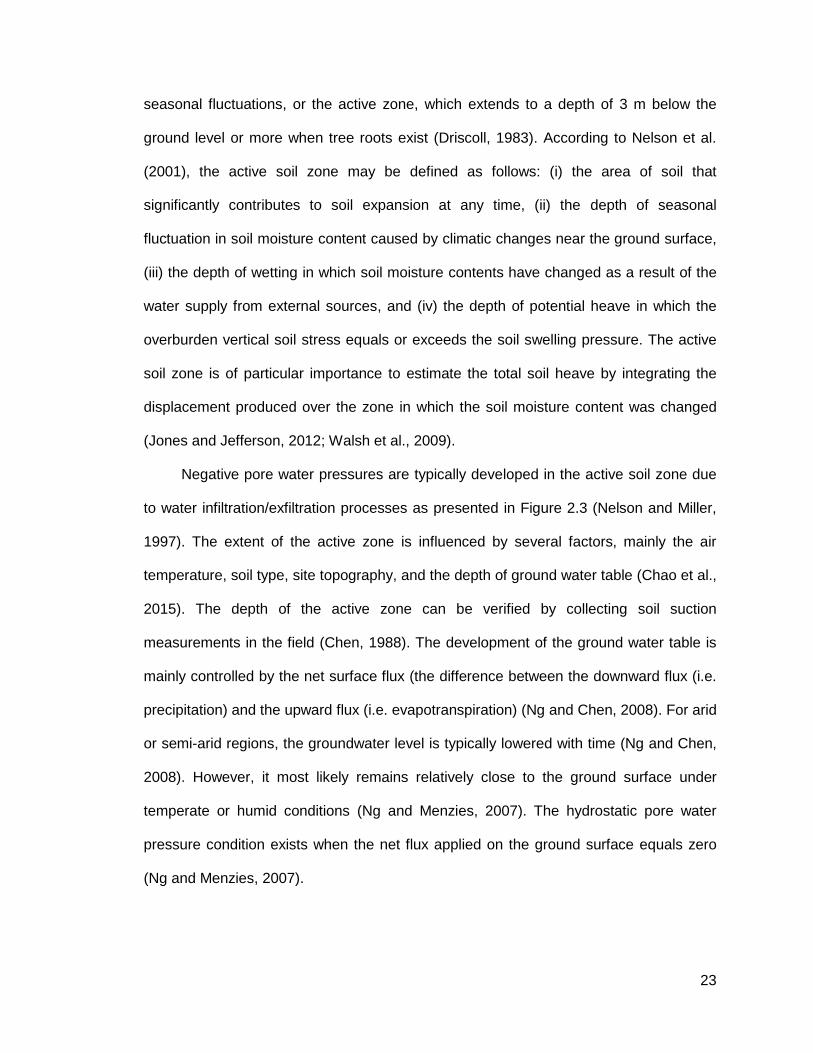
Negative pore water pressures are typically developed in the active soil zone due
to water infiltration/exfiltration processes as presented in Figure 2.3 (Nelson and Miller,
1997). The extent of the active zone is influenced by several factors, mainly the air
temperature, soil type, site topography, and the depth of ground water table (Chao et al.,
2015). The depth of the active zone can be verified by collecting soil suction
measurements in the field (Chen, 1988). The development of the ground water table is
mainly controlled by the net surface flux (the difference between the downward flux (i.e.
precipitation) and the upward flux (i.e. evapotranspiration) (Ng and Chen, 2008). For arid
or semi-arid regions, the groundwater level is typically lowered with time (Ng and Chen,
2008). However, it most likely remains relatively close to the ground surface under
temperate or humid conditions (Ng and Menzies, 2007). The hydrostatic pore water
pressure condition exists when the net flux applied on the ground surface equals zero
(Ng and Menzies, 2007).

24
Figure 2.3: A general presentation of soil mechanics principles showing the role of the
surface flux boundary condition after (Ng and Menzies, 2007)

25
2.4 Clay Mineralogy
Clay mineralogy is a primary factor controlling the swelling /shrinkage behavior of
clays. Internal surface area, charge distribution, and cation species determine the
swell/shrink potential of a clay mineral (Thomas, 1998). The most common clay minerals
consist of Kaolinite, Montmorillonite, and Illite. Clays composed of Montmorillonite
minerals are characterized by high swelling potential, high Liquid Limit, high Plasticity
Index, and less particle size compared to other clay minerals (Illite and Kaolinite). The
changes in the clay mineral composition are the primary factors for the swelling to occur
(Mitchell, 1993). The swelling action is controlled by the balancing of forces of
interaction between water, clay surface, and ions. The clay particles typically hold a net
negative charge and the larger negative charges are originated from larger specific
surfaces (Das, 2006).
Clay minerals adsorb external cations and maintain them in an exchangeable
state (Ma and Eggleton, 1999). In addition, adsorbed cations may also be replaced by
other cations which is known as the cation exchange process. The cation exchange
capacity (CEC) of soils is defined as the total number of adsorbed exchangeable cations
per 100 gms of dry soil (milliequivalent/100 gms) (Robertson et al., 1999). Swell
potential typically increases as CEC increases (Manosuthikij, 2008). Norrish (1954)
found that a montmorillonite could experience a swelling magnitude of 100% in volume
when it gets saturated with a divalent cation, such as Ca2+. The swelling potential is
influenced by the soil index properties, such as plasticity index, shrinkage limit and clay
content. Various empirical methods were established to correlate the swelling potential
to soil index properties such as Table 2.2 and Figure 2.4.
The colloid size for soils is defined as the fraction finer than 0.002 mm determined
by hydrometer analysis. Clay particles are mostly in the colloidal size range of 1mm,
where 2 mm is considered to be the upper limit (Das, 2006). The magnitude of swell

26
increases with the increase of colloid content. The plasticity index of clays increases
linearly with the percentage of clay-size fraction (% finer than 2 mm by weight)
(Skempton, 1953). Typical values of the liquid and plastic limits and specific gravity for
some clay minerals are summarized in Table 2.3. The activity of clays is defined as the
slope of the line correlating plasticity index and percentage finer than 2 µm (Skempton,
1953). Skempton (1953) identified three classes of the clay activity based on the
magnitude of the soil activity: (i) inactive (soil activity is less than 0.75); (ii) normal
(soil activity is between 0.75 and 1.25); and (iii) active (soil activity is greater than
1.25). Typical values of surface charge density, activity, and CEC for some clay minerals
are also summarized in Table 2.3.
Surficial lacustrine soil deposits in Saskatchewan were characterized by physically
powerful montmorillonitic pattern (Rice et al., 1959). Regina clay classification and
previous mineralogical tests results are illustrated in Table 2.4. The test results of
Regina clay resulted in the following mineralogical composition, approximately 53% of
montimorillonite, 35% of Illite and 12% of Kaolinite (Fredlund, 1975). Regina clay is
generally identified as montmorillonitic clay due to the high Montmorillonite content
which controls its behavior. In addition, previous test results confirmed that Regina clay
is in particular a calcium Montmorillonitic clay (Fredlund, 1975). The geotechnical
classification and mineralogical test records also confirmed the high swelling and
shrinkage potential of Regina clay. This high shrink-swell potential is resulting from the
high clay content (approximately more than 60%), and the dominance of Smectite or
Montmorillonite minerals (Anderson, 2010).

27
Table 2.2: Degree of expansion as estimated from classification test data, after (Holtz and Kovacs, 1981)
Degree of Expansion ( % - 1 µm) Plasticity
Index Shrinkage
Limit
Very High 28 > 35 < 11
High 20 - 31 25 - 41 7 - 12
Medium 13 - 23 15 - 28 10 - 16
Low 15 < 18 > 15
Table 2.3: Typical values of geotechnical index properties for the different clay minerals after (Das, 2006; Holtz and Kovacs, 1981; Mitchell, 1993; Yong and Warkentin, 1966; Zhang, 2004)
Property
Clay Minerals
Kaolinite Illite Montmorillonite
Specific Gravity, Gs 2.6 2.8 2.65 - 2.80
Plastic Limit, LL (%) 20 - 40 35 - 60 50 - 100
Liquid Limit, PL (%) 35 - 100 60 - 120 100 - 900
Cation Exchange Capacity, CEC (me/100gm)
3 - 15 10 - 40 80 - 150
Activity 0.3 - 0.5 0.5 - 1.2 1.5 - 7.0
Length and Width (mm) 0.3 - 3.0 0.1 - 2.0 0.1 - 1.0
Specific Area (m2/g) 20 - 80 80 - 100 800
Reciprocal of average surface charge density (Å2/electronic charge)
25 - 100
Swell-shrink Potential Low Medium High

28
Table 2.4: Regina clay classification and mineralogical tests results (Fredlund, 1967; Fredlund, 1975; Hu and Vu, 2011)
Property Value
Specific Gravity 2.7 – 2.8 A
tte
rberg
Lim
its
Shrinkage limit, SL (%) 13.1
Plastic limit, PL (%) 24.9 – 34
Liquid limit, LL (%) 50.6 – 94
Plasticity index, PI (%) 25.7 – 60
Gra
in S
ize
Dis
trib
utio
n Gravel sizes (≤62 mm) (%) 0 – 0.4
Sand sizes (≤5 mm) (%) 0.1 – 8
Silt sizes (%) 40.6 – 41
Clay sizes (%) 51 – 58
Cla
y
Min
era
ls
(fo
r le
ss 2
mic
ron) Kaolinite (%) 8
Illite (%) 15
Montmorillonite (%) 77
Exch
an
ge
Ca
tion
s
Magnesium (me/100 gm) 15.3
Calcium (me/100 gm) 54.4
Potassium (me/100 gm) 0.59
Sodium (me/100 gm) 1.77
CEC (me/100 gm) 31.7
Activity 7.0

29
Figure 2.4: The relationship between soil plasticity and swelling potential, after (Van Der Merwe, 1964)
0 10 20 30 40 50 60 70
Clay Fraction of Whole Sample (%2)
0
10
20
30
40
50
60
70
Pla
sticity Ind
ex (
%)
Very High
High
Medium

30
2.5 Unsaturated Soil Parameters
2.5.1 Stress State Variables
Several equations and definitions were developed to determine the effective
stresses for unsaturated soils. Previous research studies indicated that there are
significant differences between the field behavior of saturated and unsaturated soil
deposits due to the existence of matric suction (Wulfsohn et al., 1996). Therefore, the
effective stress theory of saturated soils cannot be applied directly to unsaturated soils.
Unsaturated soils were represented by three-independent phases, namely air, water and
solid (Lambe and Whitman, 2008). The contractile skin (air-water interphase) can be
considered as an independent fourth phase, which develops normal stresses due to the
pore-water pressure (Davies and Rideal, 1961). However, the contractile skin phase is
usually considered in the water phase when establishing volume-mass relationships for
unsaturated soils (Fredlund and Rahardjo, 1993b).
The stress state influences the mechanical behavior of soils. Terzaghi (1936)
established the effective stress concept for saturated soils as indicated in Equation (2.1).
(2.1)
where;
σ’ is the effective normal stress,
σ is the total normal stress, and
uw is the pore-water pressure.
Skempton (1961) modified the effective stress equation of Terzaghi to count for
the effect of soil compressibility as shown in Equation (2.2). The effective stress
principle has then been extensively used in engineering modelling and analysis to
correlate between elastic deformations and stresses of a soil structure.

31
(2.2)
where;
cg refers to the compressibility characteristic of the solid grains, and
cs refers to the compressibility characteristic of the solid skeleton.
The effective stress equation of Terzaghi did not account for some factors,
including the capillary forces, particle and pore size, pore air and pore-water pressure or
matric suction, air–water surface tension, degree of saturation and contact angle
(Fredlund and Rahardjo, 1993b). The effective stress equations for unsaturated soils
were derived from the definition of the normal inter-particle forces. The principle of
effective stress, applied in saturated soils, was found to be inadequate to express the
volumetric behavior of unsaturated soils (Matyas and Radhakrishna, 1968). The
effective stress condition in unsaturated soils, therefore, has been directly demonstrated
as a function of the total stress and the pore water pressure. The main theoretical
concept is to transfer a multi-stress medium to a single stress state continuum (Nuth and
Laloui, 2008).
Bishop (1959) also developed an effective stress equation as presented in
Equation (2.3).
(2.3)
where;
ua is the pore-air pressure,
The difference (σ-ua) is the net normal stress,
The difference (uw−ua) the matric suction ( ), and
is a parameter that is a function of the degree of saturation (S %).
= 1 for fully saturated soils and = 0 for dry soils.

32
The relationship between x and S was experimentally determined and
documented.
Another mechanistic approach was developed by (Lambe, 1960) who defined the
effective stress of unsaturated soils in terms of the inter-particle forces, as well as the
applied forces as shown in Equation (2.4).
(2.4)
where;
aa is the fraction of the total area that is air,
am is the fraction of the total area that is mineral,
aw is the fraction of the total area that is water, and
R and A are repulsive and attractive electrical forces.
Aitchison (1965) proposed a form of the effective stress equation in order to show
the relationship of matric suction and effective stress Equation (2.5).
(2.5)
where;
p" is the pore water pressure deficiency parameter, and
is a parameter that is a function of the degree of saturation ( varies from zero
to one).
Jennings (1961) modified the form of effective stress equation based on the soil suction
and a parameter β as illustrated in Equation (2.6).
(2.6)
where;
p’’ is the pore water pressure deficiency parameter, and
β is a statistical factor (β can generally be measured experimentally).

33
Richards (1967) included a new component in order to represent osmotic suction in the
effective stress equation, as illustrated in Equation (2.7).
(2.7)
where;
is an effective stress parameter,
is an effective stress parameter intended for solute suction,
hm is the matric suction element, and
hs is the solute suction element.
Aitchison (1965) published an effective stress equation based on Richards (1967)
as presented in Equation (2.8).
(2.8)
where;
P”s is the solute suction,
P”m is the matric suction, and
and are soil parameters ( and typically varies between zero and one).
Khalili and Khabbaz (1998) introduced the value of effective stress parameters through
experimental data as indicated in Equation (2.9).
(2.9)
where;
is a parameter that is a function of the degree of saturation (Khalili and Khabbaz,
1998).

34
Houlsby (1997) developed an effective stress concept to incorporate the stress and
strain variables. The equation was developed using the same form of Bishop (1959), but
through replacing the parameter ( ) with the degree of saturation as shown in Equation
(2.10).
(2.10)
where;
S is the degree of saturation, and
is a substitution factor (Houlsby, 1997).
As shown in the previous equations, the unsaturated soil behavior was found to be
better expressed using two independent stress components, normal stress and soil
matric suction (Bishop and Blight, 1963). Fredlund and Morgenstern (1976) also
reported that the volume change of unsaturated soils can be defined by any two of the
three possible stress variables, normal stress (σ – ua), matric suction, (ua – uw), and
effective stress (σ – uw). Fredlund and Rahardjo (1993b) noted that the pore-air
pressure is a significant parameter for most engineering real problems. The combination
of stress state variables, (σ – ua) and (ua – uw), has been the most extensively used
variables because the changes in total normal stress can be determined independently
of the changes in the pore-water pressure.
2.5.2 Soil Suction
Soil suction is characterized as the free energy state of soil water and is determined as
a function of the partial vapor pressure. Equation (2.11) shows the basis for measuring
the soil suction (Richards, 1965).

35
(2.11)
where;
is the total suction,
is the temperature,
is the universal gas constant,
is the specific volume of water,
is the molecular mass of water, and
is the relative humidity (presented as a decimal).
Soil suction is a vital stress component for evaluating the behavior of unsaturated
soils. Soil suction may present a significant enhancement for geotechnical engineering
analysis of earth structures (Oh et al., 2008). Croney and Coleman (1948) showed the
significant role of soil suction in identifying the mechanical behavior of unsaturated soils.
Aitchison (1965) established detailed definitions of the soil suction mechanisms. The
total soil suction of a soil can be subdivided into two main mechanisms (i.e. matric
suction and osmotic suction) (Marshall, 1958).
The matric suction is expressed as the difference between the pore-air and pore-
water pressures, ( = ua – uw), and is a function of the radius of the spherical surface
and the surface tension as shown in Equation (2.12) (Fredlund and Rahardjo, 1993b).
Matric suction is typically derived from the capillary actions associated with the surface
tension forces of the pore water within the soil structure. The surface tension is
associated with the intermolecular forces applied to the water molecules at the air-water
interface (Fredlund, 1979).
(2.12)
where;
is the matric suction,

36
is the radius of the spherical surface, and
is the surface tension.
Osmotic suction is originated from the salt concentration in the pore-water, and it
occurs in saturated and unsaturated soils (Fredlund and Rahardjo, 1993b). The
concentration of the salt solution drives an attraction to water molecules in the soil
structure. Osmotic suction reduces the energy state of water in the soil and is
associated with physico-chemical interactions between pore water and soil minerals
(Fredlund and Rahardjo, 1993b). Osmotic suction is typically considered significantly
less than matric suction and less sensitive to variations in soil moisture content
(Fredlund and Rahardjo, 1993b). Therefore, the changes in matric suction are
considered practically representative of changes in total suction for unsaturated soil.
Equation (2.13) shows the relationship between the mechanisms of soil suction
(Fredlund and Rahardjo, 1993a).
(2.13)
where;
is the total suction,
is the matric suction component, and
is the osmotic suction component.
2.6 Desiccation Cracks
Unsaturated clay soil deposits are characterized by the presence of naturally
occurring desiccation cracks. The topic of desiccation cracks phenomenon has been
covered in the past in a number of research studies (Kodikara et al., 2002; Miller et al.,
1998; Morris et al., 1992; Nahlawi and Kodikara, 2006; Yesiller et al., 2000). The
development of soil cracks influences the behavior of the near surface clay layer, and
consequently, the moisture content changes with time. The effect of desiccation cracks

37
occurring in highly plastic clay soils has been investigated and studied extensively using
different experimental methods. Albrecht and Benson (2001) found that the development
of cracks resulted in a noticeable increase in the hydraulic conductivity of clays, at times
as high as three orders of magnitude. Generally, desiccation cracks are formed because
of the soil shrinkage during the water loss process. The extent of desiccation cracks
below the ground surface has to be estimated so that it can be used an input in the soil-
weather models. The depth of cracking is often required for equilibrium analyses in
geotechnical engineering (Lau, 1987). Researchers have developed various methods to
compute the likely depth of desiccation cracking using various theoretical assumptions.
Fracture mechanics is the technical approach defining the crack propagation
criteria in materials mainly by evaluating the stress and strain fields near the crack tip
(Hanson et al., 1994). In the area of fracture mechanics, the cracking process is treated
as a mechanical process, and the cracking criterion is based on the critical stress field
(Anderson, 2005). The basic concept is that the crack propagation occurs if the energy
released upon crack growth is adequate to exceed the material resistance (Griffith,
1921). The material resistance involves the plastic work, surface energy, or other types
of energy dissipation caused by a crack (Anderson, 2005).
From a mechanical point of view, the stress distribution at the crack tip can be
assumed as presented in Figure 2.5, and therefore can be computed as a function of the
material stress intensity factor (fracture toughness) and applied tensile stress as shown
in Equations (2.14) to (2.16).
(2.14)
(2.15)
(2.16)

38
where;
r is the distance from the crack tip at inclination from the horizontal axis, and
is the fracture toughness.
The stress intensity factor (fracture toughness) was found in the literature for
clayey soils, 12.7 kPam1/2 (Ayad et al., 1997; Lee et al., 1988). The fracture
toughness can be defined as presented in Equation (2.17) (Lawn and Wilshaw,
1975a; Lawn and Wilshaw, 1975b).
(2.17)
where;
is the compression modulus,
is the Poisson's ratio, and
ζ is the specific surface energy of the soil, range, from 0.1 to 1.0 J/m2 (Lee and
Ingles, 1968).
In addition, the critical crack size is a material property specifying the size of a
crack that causes failure at a certain stress level. Consequently, the critical crack size
can vary significantly with the material type and can be defined as presented in Equation
(2.18) (Anderson, 2005).
(2.18)
where;
is the critical crack length in an infinite plate,
is a parameter dependent on the material properties and crack geometry, and
is the tensile stress.
Several studies (Blight and Williams, 1971; Briones and Uehara, 1977; Raats,
1984) applied the Griffith's brittle fracture theory on the desiccation cracking of soils. The

39
fracture toughness was defined as a mechanical parameter indicating the ability to
withstand a crack failure. This parameter was used to estimate the extent of desiccation
cracks. The relationship between fracture toughness and other mechanical parameters,
such as tensile strength, were previously examined (Wang et al., 2007). Corte and
Higashi (1964) reported that cracking by desiccation is somehow different from
mechanical cracking mainly because of the material loses mass during the process. Lau
(1987) presented a mathematical model for the determination of the cracking depth as a
function of the soil shear strength represented by the Rankine theory of lateral earth
pressure. Morris et al. (1992) proposed an analytical approach based on the linear
elastic theory to predict the cracking depth for various soil parameters and suction
values. These two methods were used to estimate the theoretical depth of cracking for
the native soils in this research study.
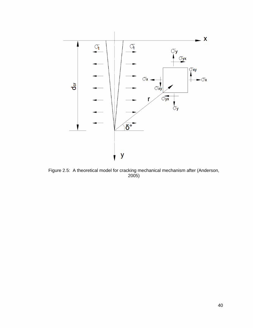
40
Figure 2.5: A theoretical model for cracking mechanical mechanism after (Anderson, 2005)

41
2.7 Hydraulic Conductivity Function
The hydraulic conductivity is a main soil property controlling the soil-water
interaction. The hydraulic conductivity for saturated soils can be assumed as a constant
value. In principle, water flows through the pore spaces containing water. Therefore, the
soil hydraulic conductivity is dependent on the water content for unsaturated soils
(Childs and Collis-George, 1950). The lower moisture content is, the lower the hydraulic
conductivity value is for unsaturated soils because of the lower availability of saturated
pores. Therefore, the hydraulic conductivity of unsaturated soil should be considered as
a function of matric suction (Gallage et al., 2013). As a general trend, the hydraulic
conductivity of soil decreases noticeably with the decrease in the degree of saturation
(Ng and Menzies, 2007).
LIoret and Alonso (1980) reported that the soil hydraulic conductivity is not
constant and is a function of volume-mass soil properties. The hydraulic conductivity
function was, therefore, expressed as the relationship between the hydraulic
conductivity and soil suction. Due to the difficulty of measuring the hydraulic conductivity
function, methodologies to estimate the physical properties of the pore space provided
insight in estimating the saturated-unsaturated hydraulic conductivity. Therefore,
prediction methods are frequently used and mostly based on the soil-water retention
characteristics (Durner, 1994). Depending on the severity of the structural changes
associated with the formation of desiccation cracks, the hydraulic conductivity may get
increased by several orders of magnitude (Johnston and Haug, 1992).

42
2.8 Soil Water Characteristic Curve (SWCC)
The soil water characteristic curve (SWCC) is a relationship between matric
suction and soil moisture condition under a normal stress of zero or (small value). The
SWCC is a critical soil property demonstrating the transient water flow through
unsaturated soils. The soil moisture characteristics may be presented in terms of
volumetric water content, gravimetric water content, or degree of saturation. SWCC
function describes the water storage capacity of a soil at various soil suctions. A review
of the literature indicated the presence of different graphical presentations for the
SWCC. Soil suction and water content (volumetric or gravimetric) can be plotted on the
abscissa, ordinate, or on a logarithmic scale. Fredlund et al. (2001) recommended that
soil suction be plotted on the abscissa and water content be plotted on the ordinate. A
standard unimodal SWCC for a drying cycle is shown in Figure 2.6.
The main parameters always identified on SWCCs are the air entry value and the
residual water content. The air-entry value is identified as the matric suction at which air
begins to go through the pores in the soil structure. The residual water content is the
water content at which a considerable amount of suction change is required to take out
any additional water from the soil structure (Fredlund and Xing, 1994). The residual
water content may be determined as the intersection of two lines, a tangent line drawn
from the inflection point and a tangent line drawn from the high-suction range as shown
in Figure 2.6 (Fredlund and Rahardjo, 1993b). The soil suction at a water content of zero
value was found to be approximately 106 kPa (Fredlund and Xing, 1994). White et al.
(1970) identified three main de-saturation stages along the drying curve, namely the
boundary effect phase, the transition state, and the residual stage. Similar stages of
saturation were found to be applicable to the wetting curve (Fredlund, 2000).
43
The most commonly known shape of the SWCC is the unimodal SWCC which
contains two bending curves only. The capacity of fine-grained soils to retain water
depends on the soil fabric including macropores, mesopores, and micropores (Elkady,
2014; Mitchell, 1993). The soil native structure and grain size distribution are
contributing factors affecting the nature of the SWCC (Fredlund and Rahardjo, 1993b;
Vanapalli et al., 1998). Recent research studies have shown bimodal SWCCs with two
distinct structures of the pore size distribution (de FN Gitirana Jr and Fredlund, 2004;
Satyanaga et al., 2013; Zhang and Chen, 2005). Bimodal SWCCs are typically observed
in the case of soils with cracks, and it can be utilized to simulate the changes in soil
water content in the field. The bimodal curve defines two air entry values and two
residual volumetric water contents including near horizontal or horizontal intermediate
segment (Elkady, 2014).

44
Figure 2.6: Typical soil water characteristic curve of clay soil
Matric Suction, (kPa)
Volu
metr
ic W
ate
r C
onte
nt,
(a,s)
(r,r)
Air-Entry Value (AEV)
Residual Volumetric Water Content
Saturated Volumetric Water Content
45
2.9 Measurements of Soil Moisture-suction Characteristics
2.9.1 Foreword
Measuring the soil-water characteristics using field instrumentation is essential in
understanding the behavior of underground structures and the soil-water interaction
(Fredlund, 2006). Monitoring the soil-water characteristic in the field is an efficient tool to
validate the results of the numerical studies. Various types of instruments are employed
in measuring the soil water characteristics. These methods determine the soil moisture
using calibrated relationships derived from other measurable parameters (Muñoz-
Carpena et al., 2004). The suitability of each method relies on a number of aspects (i.e.
cost, installation, accuracy, purpose, response time, management and durability) (SAI
Platform, 2010). Primary methods and techniques normally utilized for measuring the
soil-water characteristics are classified into volumetric and tensiometric techniques as
shown in Figure 2.7, and discussed in the following subsections.
2.9.2 Soil Moisture Monitoring (Principle and Techniques)
There is a range of readily available techniques for the determination of soil
moisture conditions. The moisture content of a given soil can be measured through
direct and indirect techniques (Muñoz-Carpena et al., 2004). The direct measuring
technique can be achieved through a thermo-gravimetric technique (i.e. weight of water
over the weight of dry soil) or a thermo-volumetric technique (volume of water within a
volume of undisturbed soil) (Muñoz-Carpena et al., 2004). These direct techniques are
laboratory based methods and, therefore, are accurate and inexpensive. However, they
are destructive, time-consuming and cannot be used to monitor the moisture content in
the field (Agricultural Technology Centre, 2004).

46
Various field monitoring techniques (i.e. indirect techniques) were developed for
measuring the soil volumetric water content in the field (SAI Platform, 2010). It is
essential to understand the differences between these available techniques in order to
choose the most suitable instrument for the proposed function. All the volumetric
measuring methods measure the volume of water within a volume of undisturbed soil
(SAI Platform, 2010). The available techniques include neutron moderation technique,
dielectric techniques, and other techniques (such as Ground Penetrating Radar (GPR),
Gamma Attenuation, Nuclear Magnetic Resonance, Capacitive Sensor, and Optical
Methods) (Muñoz-Carpena et al., 2004). Table 2.5 provides an evaluation of the most
common water measurements techniques. Amongst these available methods, the
Neutron moderation, Time Domain Reflectometry (TDR), Water Content Reflectometry
(WCR), Frequency Domain Reflectometry (FDR), Amplitude Domain Reflectometry
(ADR) methods can be used for research purposes (Muñoz-Carpena et al., 2004). The
neutron moderation apparatus estimates the volumetric water content by measuring the
thermal density or the slowed neutron density (Agricultural Technology Centre, 2004) .
The neutron moderation is derived from a linear calibration between a probe reading ,
and the measured soil moisture content using field samples (Muñoz-Carpena et al.,
2004). This technique may be used to assess the soil moisture at various depths below
the ground surface (SAI Platform, 2010).
Dielectric methods are widely used to monitor soil volumetric water content in
coarse-grained or fine-grained soils with low to medium plasticity (Hu et al., 2008).
These methods consist of the time domain reflectometry (TDR), the water content
reflectometry (WCR), the amplitude domain reflectometry (ADR), and the frequency
domain reflectometry (FDR) (Muñoz-Carpena et al., 2004). The dielectric techniques
utilize empirically verified relationships between the volumetric water content and the
sensor output magnitude (mainly time, frequency, impedance and wave phase) (Muñoz-
47
Carpena et al., 2004). These generic calibration relationships were developed for typical
soils and are sensitive to the soil mineralogy, bulk density and temperature. The use of
dielectric techniques in highly plastic, unsaturated, expansive clay soil is limited, and
therefore, soil-specific calibrations are considered necessary (Hu et al., 2008).
2.9.3 Soil Suction Monitoring (Principle and Techniques)
Tensiometer systems are methods for measuring the energy holding water in soils
(Muñoz-Carpena et al., 2004). Tensiometers are devices for determining the energy of
the soil solution (known as, the soil water matric potential) (Soil Science Society of
America, 2008). They are typically able to monitor the soil tension variations occurring
during different seasonal event such as infiltration, irrigation, groundwater recharge and
evapotranspiration processes (Agricultural Technology Centre, 2004). Tensiometers
consist of three essential elements, a porous cup, a water reservoir, and a measurement
gauge (Young and Sisson, 2002). Tensiometers generally require the gauge to reach
equilibration with the soil moisture. Table 2.6 provides an evaluation of the most
common tensiometric techniques. Amongst the available methods, tensiomneters, heat
dissipation, and soil pyschrometers are the ones which can be used for research
purposes (Muñoz-Carpena et al., 2004). Tensiometers may or may not get affected by
osmotic or gravitational potentials depending on the manufacture (Young and Sisson,
2002). The soil water potential measured by a tensiometer always captures the matric,
pneumatic and overburden potentials (Young and Sisson, 2002). Generally, tensiometer
systems may not require a soil specific calibration/validation, however, they may have to
be installed permanently, or at least a sufficient time period has be provided in order to
develop equilibration between the tensiometer and soil before retrieving the readings
(Agricultural Technology Centre, 2004).

48
Figure 2.7: Measurement methods of soil-water characteristics

49
Table 2.5: Evaluation criterion for volumetric soil water monitoring techniques (Muñoz-Carpena et al., 2004)
Specification Neutron TDR/WCR FDR ADR Phase
Transmission
TDT
Reading range
0 - 0.60
0.05 - 0.50 or
0.05 - Saturation (with soil specific
calibration)
0 - Saturation 0-Saturation 0.05-0.50
0.05 - 0.50 or
0 - 0.70 Depending
on instrument
Accuracy (considering soil specific calibration)
±0.005 ±0.01 ±0.01-0.05 ±0.01 ±0.05
Installation technique
Access Tube
Permanently
buried in the field
or inserted for
manual readings
Permanently buried in the field or PVC access
tube
Permanently buried in the
field or inserted for
manual readings
Permanently buried in the field
Logging capacity
No Depending on
instrument Yes
Influenced by salinity
No Yes Minimal No >3 dS/m Yes
Not commonly used for
None
Organic,
dense, salty or
high clay content
soils (depending
on instrument &
calibration)
None None None
Organic,
dense, sallty or high clay content soils (depending
on instrument & calibration)
Field maintenance
No
Safety hazard Yes No
Applications Irrigation, Research, Consultants Irrigation, Research Irrigation

50
Table 2.6: Evaluation criterion for soil suction monitoring techniques (Muñoz-Carpena et al., 2004)
Specification Tensiometer Gypsum Block GMS Heat
Dissipation Soil
Psychromotor
Reading range
0 - 0.80 bar 0 - Saturation 0-Saturation 0.05-0.50
0.05 - 0.50 or
0 - 0.70 Depending on the
instrument
Accuracy, bar (considering soil
specific calibration) ±0.01 ±0.01 ±0.01-0.05 ±0.01 ±0.05
Installation method
Get inserted into hole permanently
Logging capacity Only when
using transducers
Yes
Influenced by salinity
No >6 dS/m >6 dS/m No Yes for
(ceramic type)
Not commonly used for
Sandy or coarse soils
Sandy or coarse grained soils
swelling clay
Coarse soils
Sandy or coarse grained
soils
swelling clay
Maintenance Yes No Medium No No
Safety hazard No
Applications Irrigation, Research
Irrigation Irrigation, Research
Research

51
2.10 Unsaturated Soil-atmosphere Interaction
2.10.1 Foreword
The main objective of soil-atmosphere transport models is to determine and
evaluate the soil exchange fluxes between soil and atmosphere. Soil-atmosphere
interaction models involve the estimation of the rates of heat and moisture flow through
the soil structure. The boundary conditions depend on two principal components,
evaporation (or evapotranspiration) and precipitation. Evaporation is related to free
water surfaces while evapotranspiration is associated with wet soil surfaces (Veihmeyer,
1964). The following subsections discuss the soil evaportranspiration process, and
water and heat flow through soil structures.
2.10.2 Soil Evaportranspiration
The understanding of the evapotranspiration process was established in the
1940’s (Gitirana Jr, 2005). Early studies reported that the evapotranspiration process
occurs under three main conditions: (i) a continuous supply of energy should be existing
for the latent heat of vaporization, (ii) the vapour pressure of the atmosphere above the
surface should be less than the vapour pressure at the soil surface, and iii) the vailability
of a continual supply of water to the evaporating surface (Baver et al., 1972; Hillel, 1982;
Penman, 1948; Veihmeyer, 1964; Wilson, 1990). For soils, the provision of water is
influenced by soil conditions (i.e. soil properties, moisture content, and groundwater
table). Generally, the shallower the groundwater level is, the higher the
evapotranspiration rate (Gardner, 1958).
A detailed review of the equations for calculating the potential evapotranspiration
(PE) can be found in (Wilson, 1990). Penman (1948) developed an equation that is a
very popular one for indirectly estimating potential evapotranspiration. This equation
takes into consideration the effect of a number of essential meteorological factors (i.e.

52
air temperature, relative humidity, net solar radiation and wind speed). Modified forms of
this equation were also developed by different scholars in subsequent publications
(Black, 2007). Wilson (1990) and Wilson et al. (1997) developed partial differential
equations for calculating evapotranspiration fluxes from saturated/unsaturated soils. The
approach was experimental in nature, but had a sound theoretical basis, and was
therefore adopted in this research work.
2.10.3 Water Flow
The main concept of modeling of the in/exfiltration flux into soils was developed
based on the law of conservation of mass. The total mass of water per unit volume of
the soil medium can be presented as shown in Equation (2.19).
(2.19)
where;
is the water density (998.2 kg/m³);
θ is the volumetric moisture content (vol/vol),
ρv is the vapour density (kg/m³), and
θa is the volumetric air content (vol/vol).
Mass conservation would then result in Equation (2.20).
(2.20)
where;
t is the time, and
qm is the total moisture flow (kg/m²s).
The hydraulic head gradient can be expressed as the driving force of water to flow
through the soil structure from points of high head to points of low head. Other
driving forces include moisture content and matric suction gradients. However, these
gradients do not fundamentally govern the water movement through the soil structure

53
(Fredlund and Rahardjo, 1993b). The flow net technique was initially used for predicting
seepage through earth assuming that water only flows below the ground water table
(Casagrande, 1937). Finite element methods have alternated the flow net technique due
to their powerful nature. Due to the complexity of modeling seepage in
saturated/unsaturated soils, It is viable to employ general partial differential equation
solvers (Nguyen, 1999). The water flow rate in saturated/unsaturated soils can be
identified using a generalisation of Darcy’s Law, where the total head gradient and the
hydraulic conductivity are functions of matric suction (Bear, 1972; Fredlund and
Rahardjo, 1993b). The generalised Darcy’s law may be expressed as shown in Equation
(2.21).
(2.21)
where;
and are liquid pore-water flow rates in the x- and y- direction across a unit
area of the soil due to the hydraulic head gradients (m3/m2s),
, and are hydraulic conductivity (m/s) in the x-, and y- direction, and
is the total hydraulic head (m).
In the field, piezometers are used to provide a measurement of the water head in
saturated soils. The hydraulic conductivity is approximately constant for saturated soils.
Above the water table, the pressure heads are negative, and the hydraulic head can be
determined indirectly through the field measurement of the suction head or negative
pore-water pressure. Childs and Collis-George (1950) reported that water flows only
through the pore spaces filled with water and the soil hydraulic conductivity is a function
of the soil suction for unsaturated soils. Under unsaturated soil conditions, few saturated

54
pores are available for water to flow, and consequently, the lower moisture content is the
lower the hydraulic conductivity value.
LIoret and Alonso (1980) reported that the soil hydraulic conductivity is not
constant and is dependent on volume-mass soil properties. The hydraulic conductivity
function was, therefore, defined as the relationship between the hydraulic conductivity
and soil suction. During the de-saturation process of soil, air begins to enter the large
pore spaces first, and water flow is forced to move along the more tortuous path
in the smaller soil pores. The hydraulic conductivity decreases rapidly as the volume of
pore space occupied by water decreases. Although Darcy’s law was developed for
predicting the flow in saturated soils, it was then applied to the flow of water through
unsaturated soil with the consideration of the change in the hydraulic conductivity
(Richards, 1931). There are different versions of Richards’ equation for the
determination of moisture movement through saturated-unsaturated soils. All these
versions were mainly based on calculating water continuity in terms of matric suction.
Equation (2.22) illustrates the two-dimensional partial differential form of Richards’
equation.
(2.22)
where;
is the total hydraulic head (m),
kx is the hydraulic conductivity (m/s) in x-direction,
ky is the hydraulic conductivity (m/s) in y-direction, and
θ is the volumetric water content (VWC) (vol/vol).
Fredlund and Rahardjo (1993a) presented a general partial differential equation derived
from Richards’ equation for the transient moisture flow through saturated/unsaturated
soils as shown in Equation (2.23).

55
(2.23)
where;
h is the total head (m),
is the slope of the soil water characteristic curve, and
is the unit weight of water (kN/m3).
2.10.4 Heat Flow
Soil temperature is a critical factor controlling many physical processes or changes
that take place in soils. Soil temperature changes are attributable to the changes in
radiant, thermal and latent energy exchange processes (Hillel, 1982). These processes
are controlled by a complex series of heat transfer actions (i.e. radiation, conduction,
convection, advection, and phase change) known as latent heat transfer or evaporation
(Rutten et al., 2010). The heat flow element of greatest concern is the conductive heat
flow. In soils, convection heat transfer of the pore-fluid is noticeably less than conductive
heat transfer (Milly, 1984) and, therefore, can generally be neglected.
The differential form of Fourier's Law has been widely used to compute the vertical
heat flux in materials (Fourier, 1878). Differential equations for the conservation of heat
in soils were developed, taking into consideration the flow rates in and out of the soil
elemental volume, and corresponding to the difference in the rate of change in heat
stored with time (Fredlund and Gitirana Jr, 2005). The main factor in the heat flow
equation that describes the soil’s ability to transfer heat is the thermal conductivity. The
thermal conductivity of soils was found to be significantly influenced by the degree of
saturation and dry density (Fricke, 1997). As a general trend, an increase in the degree
of saturation or dry density results in an increase in thermal conductivity (Fricke, 1997).
Other factors that have a secondary effect upon soil thermal conductivity include frozen

56
versus unfrozen soil conditions, mineral composition and texture (Becker et al., 1992;
Fricke, 1997; Mitchell, 1991).
Different correlations for estimating the soil thermal conductivity were developed
for both coarse- and fine-grained soils (De Vries, 1952; Johansen, 1975). Al
Nakshabandi and Kohnke (1965) reported that the thermal conductivity of soils at the
same moisture condition is highest in granular soils (gravel and sand), intermediate in
loam, and lowest in clay soils. Kersten (1949) tested various soil types and developed
equations for frozen and unfrozen silt-clay soils and sandy soils. Canadian Geotechnical
Society (1978) provided a generalized basis for estimating the thermal conductivity of
frozen soils based on Kersten's research and was adopted in this research to estimate
the initial thermal conductivity for the top clay soil layer.
2.11 Unsaturated Soil-structure Interaction
2.11.1 Numerical Approaches
The main technical aspects of modeling the soil-structure interaction under
unsaturated soil conditions include the degree of simplicity, practicality to buried
structures, insufficiency of site local specific parameters and field verifications, and lack
of knowledge of some features. Soil behavior can generally be described by constitutive
relationships. Soil behavior can be described by constitutive relationships as a function
of stress state variables. The constitutive relationships provide a framework for
understanding how soil behaves under different loading conditions, and can be
formatted in finite element and finite difference codes for use in numerical analysis.
Modeling of the volume change of unsaturated soils consists of stress-deformation
analysis under mainly water and heat flow processes. The volume change behavior of
unsaturated soil can be modeled using coupled or uncoupled approaches.

57
In the uncoupled approach, the water seepage equation (adsorption-drainage
processes) is solved separately from the stress-deformation equations (mechanical
behavior) (Corapcioglu, 1984). For the seepage analysis, the dependent variable is the
hydraulic head. However, for the stress-deformation analysis, the dependent variables
are the horizontal and vertical displacements. In the coupled approach, however, the
water seepage equation and the equilibrium equations are solved simultaneously
(Pham, 2005). Previous research results showed that the outcome of uncoupled
solutions compared well with those from the coupled solutions, and uncoupled solutions
are adequate for the analysis of most volume change problems related to unsaturated
expansive soils (Vu and Fredlund, 2004).
2.11.2 Volume-mass Constitutive Relationships
A number of volume-mass constitutive models have been developed for
unsaturated soils (Pham, 2005). The typical constitutive relationships for unsaturated
soils were expressed as an extension of the saturated soil constitutive equations and
incorporated the use of two independent soil properties (total normal stress and soil
suction). The development of constitutive models for unsaturated soils is directly related
to the unsaturated soil stress variables. The stress state variables for an unsaturated
soil are generally interpreted from possible combinations of the total stress, σ, the pore-
air pressure, ua, and the pore-water pressure, uw. The combination of net stress (σ – ua),
and matric suction (ua – uw) presented in Figure 2.8 are the most widely one (Fredlund
and Vanapalli, 2002; Fredlund and Rahardjo, 1993a). Tensors for these two
independent stress variables can be formulated as shown in equations (2.24) and (2.25)
(Fredlund and Rahardjo, 1993b).

58
(2.24)
(2.25)
where;
The three normal stress parameters ( , , and ) are mutually
orthogonal with respect to x-, y- and z- direction, and
The six shear-stress parameters ( act on the i plane and on the j direction.
Volume change of unsaturated soils can occur as a result of changes in the total
stress, the matric suction, or a combination of the two cases. Fredlund and Rahardjo
(1993a) presented the theoretical basis for developing the volume-mass constitutive
surfaces for saturated-unsaturated soils. The change in void ratio as a deformation
(volume change) state variable for saturated soils was defined as a function of the net
normal stress as presented in Equation (2.26). Both void ratio and gravimetric water
content for unsaturated soils were defined as functions of the net normal stress and soil
suction as presented in Equations (2.27) and (2.28) (Fredlund and Rahardjo, 1993a).
Using these definitions, the constitutive relationships (equations) can be plotted as
surfaces on a three-dimensional graph, with each abscissa representing a stress state
variable, and the ordinate representing the soil volume-mass property as presented in
Figure 2.9 (Fredlund and Rahardjo, 1993a).
σ (2.26)
σ (2.27)
σ (2.28)

59
where;
is the change in void ratio,
is the change in water content,
is the coefficient of compressibility,
is the coefficient of compressibility as a function of the change in net normal
stress, σ ,
is the coefficient of compressibility as a function of the change in matric
suction, ,
is the coefficient of water content change as a function of the change in net
normal stress, σ , and
is the coefficient of water content change as a funtion of the change in matric
suction, .
The development methods of the volume change principle for unsaturated soils
were presented in (Fredlund and Rahardjo, 1993b). Alonso et al. (1990) established the
volume change constitutive relationships for unsaturated soils based on the net stress
and soil suction. The prediction of volume change is based on the relationship between
vertical strain (i.e. void ratio) and the logarithms of soil suction or net normal stress (Vu
and Fredlund, 2004). The fundamental concept is that the total volume change of
unsaturated soils is equivalent to the summation of volume change magnitudes
associated with the air and water phases (Fredlund and Morgenstern, 1976). The overall
volume change of unsaturated soil components can be described as shown in Equation
(2.29) (Fredlund and Rahardjo, 1993b).
(2.29)
where;
V is the total volume,

60
Vw is the volume of water, and
Va is the volume of air.
Due to the difficulty in the determination of the air volume changes in the soil
structure, the practical way is to predict the change in overall and water volumes. The
displacements associated with the change in total soil volume can then be computed as
the sum of the normal strains as presented in Equation (2.30) (Fredlund and Rahardjo,
1993a). The normal strain in a given direction, ε, is computed as the change in length
per unit length of a line. Shear strain, ζ, is, however, formulated as the change in the
right angle between referenced axes (Chou and Pagano, 1992). The relationships
between the normal and shear strains and displacements in x, y, and z directions are as
illustrated in equations (2.31) and (2.32) (Fredlund and Rahardjo, 1993b).
(2.30)
(2.31)
(2.32)
where;
is the volumetric strain,
are the normal strain components in x-, y-, and z- direction, respectively,
is the shear strain, and
are the displacements in x-, y-, z- direction, respectively.
The main principles for establishing the volume change models were based on
either the elasticity theory or empirical models. The empirical models are derived from
mathematical models fitting the relationship between stress state variables obtained
from laboratory tests measurements. The elastic models, however, are based on
relevant parameters (i.e., modulus of elasticity and Passion's ratio) and are relatively
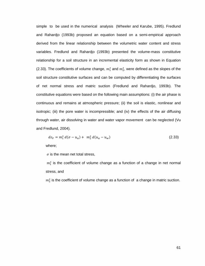
61
simple to be used in the numerical analysis (Wheeler and Karube, 1995). Fredlund
and Rahardjo (1993b) proposed an equation based on a semi-empirical approach
derived from the linear relationship between the volumetric water content and stress
variables. Fredlund and Rahardjo (1993b) presented the volume-mass constitutive
relationship for a soil structure in an incremental elasticity form as shown in Equation
(2.33). The coefficients of volume change, and
, were defined as the slopes of the
soil structure constitutive surfaces and can be computed by differentiating the surfaces
of net normal stress and matric suction (Fredlund and Rahardjo, 1993b). The
constitutive equations were based on the following main assumptions: (i) the air phase is
continuous and remains at atmospheric pressure; (ii) the soil is elastic, nonlinear and
isotropic; (iii) the pore water is incompressible; and (iv) the effects of the air diffusing
through water, air dissolving in water and water vapor movement can be neglected (Vu
and Fredlund, 2004).
(2.33)
where;
is the mean net total stress,
is the coefficient of volume change as a function of a change in net normal
stress, and
is the coefficient of volume change as a function of a change in matric suction.

62
Figure 2.8: The unsaturated soil stress state parameters using the combination of (σ – ua), and matric suction (ua – uw) (Fredlund and Vanapalli, 2002)
Figure 2.9: Constitutive surfaces for an unsaturated, swelling soil (Fredlund and Rahardjo, 1993b)
Normal S
tress
Soil Suction
Volume Change
Swell-Shrink Relationship
Consolidation Relationship

63
2.12 Pipelines Infrastructure
Buried pipes are vital infrastructures and are typically used to transport energy
and other essential commodities. Pipeline systems have improved the standard of living
and have rapidly grown in use over the last 60 years. The failure of underground
pipelines occurs when the applied stresses exceed its structural resiliency. A
comprehensive analysis of buried pipes should consider pipe characteristics, internal
and external loads, and surrounding conditions such as backfill and side fill materials,
installation depth, compaction quality, and road superstructure loads. Pipes can be
classified as either flexible or rigid, depending on whether they can deform up to 2%
without incurring damage (Suleiman, 2002).
Rigid pipes, such as reinforced/non-reinforced concrete, and clay pipes, may
experience significant structural cracks if they deflect more than 2% (Zhao et al., 1998).
Flexible pipes have been defined as conduits that can deflect at least 2% without
exhibiting any sign of structural distress such as cracking (Uni-Bell PVC Pipe
Association, 1991). Flexible pipes include thermoplastics [i.e., Polyvinyl Chloride (PVC)
and High Density Polyethylene (HDPE)], thermosetting, and corrugated steel pipes. The
relatively low cost and high processability of PVC make it the material of choice for
various industries.
Soil-pipe interaction differs between flexible and rigid pipes. A rigid pipe is
responsible for transferring the applied loads to the bedding material. Rigid pipes are
generally stiffer than the surrounding soil (Zhao et al., 1998). Flexible pipes support the
applied vertical loads through passive pressures induced by the pipe deformation
against the surrounding soils (Moser, 1990). Flexible pipes have less inherent stiffness
when compared to rigid pipes. Therefore, flexible pipes usually require efficient
compaction of the backfill soils during installation. The design of buried pipes in North
America began in the early 1900s, initiated mainly by Marston and Anderson (Marston

64
and Anderson, 1913). The design criteria of buried PVC pipes incorporate the
determination of sufficient pipe stiffness to resist buckling. Pipe deformation must be
limited to eliminate any disruption in the flow or joint leakage (American Water Works
Association, 2002). General design guidelines for underground PVC pipes can be
summarized as follows: (i) limiting the pipe deformation to a maximum of 3% [i.e.
thermoplastic pipe (Zhao et al., 1998)], and 5% to 7.5% [i.e. PVC pipes (Eagle, 2009),
based on the pipe working pressure]; (ii) preventing buckling of the pipe wall; and (iii)
limiting any potential for ‘wall crush’ that may occur due to vertical loads (soil and live
loads) applied directly above the pipe.
Pipes must have sufficient strength to achieve its intended function. Pipe strength
is the ability to resist stresses, mainly internal pressure, soil pressure, live loads, and
longitudinal bending moments/stresses. Pipe stiffness describes the load-deformation
characteristics of flexible plastic pipes, thus can be used to determine the deformations
of the pipe wall. The pipe durability, however, is the ability to resist corrosion, abrasion
and deleterious environmental conditions, and it is a significant parameter for
determining the design service life for the performance of any pipe type.
2.13 Applied Loads on Buried Pipes
2.13.1 Foreword
The loads borne by the pipes depend primarily on the pipe type. For rigid pipes,
the pipe is expected to resist any vertical pressure as well as any horizontal reacting
earth pressure. However, flexible pipes affected by vertical loads experience
deformations resulting in a supporting horizontal soil pressure (Moser, 1990). Typical
loads applied on buried pipes can be classified into dead and live loads. Dead loads
generally remain static throughout the life of the pipes, and it considers any sole dead

65
load. On the other hand, live loads always change in position and/or magnitude. The
most common live loads borne by pipes are vehicular loads (i.e., trucks or trains).
The design of any buried pipe system should consider both types of superimposed
loads, dead loads and live loads as separate design parameters (American Water
Works Association, 2002). The level of soil stresses on the pipelines depends mainly on
the soil nature soil, its degree of saturation, and other relevant factors, such as seasonal
meteorological variations, which cause periodical changes in soil moisture. It should be
noted that the superimposed loads on the underground pipes can vary significantly
throughout the life of the pipeline due to the rise of any of the following conditions
construction/ installation conditions, routine operational conditions, and extreme loading
conditions, such as landslides, and earthquake-induced ground movements
(Wijewickreme and Weerasekara, 2010).
2.13.2 Soil Load
Design earth loads can be determined using the Marston load theory (Marston,
1930). According to the theory, it was assumed that the weight of the backfill partly
resisted by frictional shear forces at the trench walls developed with time. In addition,
the apparent cohesion of the soil was ignored when determining the equilibrium of
vertical forces (Moser, 1990). Marston load theory determined the load on a buried pipe
based on the soil column weight, or central prism, which was modified by a factor that
incorporated the effect of the relative movement between the side columns of soil, or
external prisms to the central prism (Marston and Anderson, 1913). The frictional forces,
between soil prisms, can then be determined using Rankine’s theory. The soil load
applied to buried pipe for rigid pipes was determined as shown in Equations (2.34) and
(2.35). Values of the ratio of lateral to vertical earth pressure and coefficient of friction
against sides of the trench were previously estimated for different typical soil types

66
(Moser, 1990). The coefficient of friction generally ranged from 0.3 to 0.5, which
corresponded to the angle of friction values ranging from 17o to 27o (Moser, 1990).
(2.34)
(2.35)
where;
ws is the soil load on a buried pipe,
is the unit weight of backfill,
W is the horizontal width of the pipe trench,
Cd is a load coefficient for the trench,
’ is the coefficient of friction between backfill and sides of trench,
K is the ratio of active lateral pressure to vertical pressure, and
H is the height of backfill on top of the pipe.
The load on flexible pipes was found to be different from rigid pipes. It can be
determined if the relative stiffness of pipe and backfill is reasonably estimated
(Cameron, 2005). Theoretically, when both stiffnesses of soil and pipe are assumed to
be equal, then the load can be approximated to the prism load. The prism load can be
computed by the weight of the soil column directly applied above the pipe as shown in
Equation (2.36). The prism load neglects any external factors acting on pipes, such as
side wall friction. Therefore, the prism load approach can be used as a conservative
approach for flexible pipes (American Water Works Association, 2002). The actual load
on pipe may be more or less than the prism load based on the soil-pipe stiffness. When
the pipe stiffness is less than the soil stiffness, which is common for flexible pipes, the
soil above the pipe redistributes the load away from the pipe into the soil (Petroff, 1990).

67
(2.36)
where;
P is soil prism load on the pipes at a depth of H due to soil weight.
Most of flexible pipes would fall into the case of which the load imposed on the
pipe is less than the soil prism load over the pipe as shown in Equation (2.37) (Moser,
1990). For comparison purposes, the ratio of soil load applied on a flexible pipe to a rigid
pipe can be calculated as shown (2.38) which is equal to the ratio of the pipe diameter to
the trench width.
(2.37)
(2.38)
where;
D is the outside diameter of the pipe,
W is the horizontal width of the pipe trench, and
Cd is the load coefficient for the trench.
2.13.3 Live Loads
The live load is the other type of loading acting on underground pipes. Pipelines
underneath roads or railways also experience live loads. The live loads can be classified
into two types, concentrated live loads (such as a truck wheel), or distributed live loads
(Moser, 1990). The effect of live loads on a pipe decreases as the depth of soil cover
increases. The determination of live load is important for underground pipes with shallow
depths (such as less than 1.5 m) (American Water Works Association, 2002). The
method developed by Hall and Newmark (1978) uses a load coefficient (Cs) for
calculating concentrated loads as shown in Equation (2.39). The loaded surface area is
considered as a rectangle, and a truncated pyramid is punched through as what can be
determined by Equation (2.40) (Watkins and Anderson, 1999).

68
(2.39)
(2.40)
where;
Wsc is the live load on pipe due to a concentrated load,
Wsd is the live load on pipe due to a distributed load,
P is a concentrated surface load,
Pd is the intensity of a distributed surface load,
F is the impact factor,
Cs is a load coefficient, and
L is effective length of the pipe (1 m is typically used).
2.14 Pipe Stresses
Figure 2.10 shows the three principal stresses in a pipe, namely longitudinal stress
(σx) circumferential or tangential stress (σy), and radial stress (σz). According to most
design practices of pipelines, the radial stress σz is negligibly small (Young et al., 2011).
The major stresses σx and σy are considered uniform throughout the thickness of the
wall as the pipe thickness is much smaller than the pipe diameter, especially when the
ratio of the mean pipe radius to the wall thickness is more than 10.
Tangential stresses and associated bending moments are typically caused by pipe
crushing under the application of external loads. Rigid pipes and many flexible pipes
are not designed to resist high longitudinal stresses (Moser, 1990). Any uniform axial
compressive stress can produce a uniform axial tensile stress on the pipe wall as
illustrated in Figure 2.11 (Ng, 1994). Longitudinal stresses can also be produced by
different loading and environmental actions, including thermal expansion and
longitudinal bending. Longitudinal bending occurs when pipes are bent due to any
directional changes as shown in Figure 2.12 (Ng, 1994).

69
Figure 2.10: Principle stresses of a pipeline (Ng, 1994)
Figure 2.11: Stresses in a pipeline under longitudinal extension (Ng, 1994)
Figure 2.12: Stresses in a pipeline under longitudinal bending conditions (Ng, 1994)

70
2.15 Pipe Deformations
2.15.1 Horizontal Deformation
Spangler (1941) reported that flexible pipes provide limited inherent stiffness
compared to rigid pipes. By using laboratory testing results, Spangler handled the
influence of surrounding soils on the change in pipe shape as illustrated in Equation
(2.41) that is known as developed Iowa Formula. The determination of the pipe
deformation was based on the “ring theory”, assuming that the loss in vertical diameter
is compensated by an increase of the same magnitude in the horizontal diameter,
whereas the deformed pipe shape is elliptical as shown in Figure 2.13 (Moser, 1990).
This basic assumption imposes the importance of using advanced finite element
analysis and methods to better evaluate the actual behavior of pipelines.
The pipe deformation is expressed as the ratio of vertical deformation to horizontal
enlargement of the pipe diameter. The soil load in Iowa Formula can be determined
using the definition of the soil column load on underground pipe developed by (Marston
and Anderson, 1913).
(2.41)
where;
is the change in pipe diameter (flexible pipe),
is a deflection lag factor,
is the bedding constant,
Ep is the elastic modulus for the pipe material (kPa),
I is the moment of inertia of the pipe wall per unit length (m3),
E is the modulus of passive resistance of soil (kPa),
r is the mean pipe radius (m), and

71
is the soil load on the buried pipe (kN/m).
Spangler’s equation (Iowa Formula) was based on three main assumptions as follows:
The vertical deformation is equivalent to the horizontal deformation,
The pipe deformation is elliptical, and
The modulus of soil reaction is considered constant for the backfill material.
In the case of sustained loading conditions, the deflection lag factor (Dl) was found to
increase with time (Howard, 1985). Prevost and Kienow (1994) reported that the angle
of bedding support may be assumed around 90° in the determination of the deformation
and moments at a bedding constant (K) value of 0.012.
2.15.2 Bending Displacement
There are different loads that may produce axial bending stresses in a pipe. Some
of the major causes of bending displacements include the following (Moser, 1990);
The differential settlements of the structure that is directly connected to the pipe;
Settlements of the pipe bedding (i.e., erosion of the soil),
Seasonal rise and fall of soil,
Non-uniform foundation conditions, and
Tree-root growth induced pressure.
These loads can be significant, highly variable, and localized and can cause damages to
underground pipeline networks as being discussed in the following section. Figure 2.14
shows a mechanism of pipe bending displacement.

72
Figure 2.13: Pipe deformation diagram (Ring Theory)
Figure 2.14: Pipe displacement due to axial bending

73
2.16 Buried Pipe Damages
2.16.1 Failure Mechanisms Associated with Soil Movements
Failure in pipes is typically defined as a state attributable to break, collapse, or
bending so that the structure no longer fulfills its purpose even though there is no
catastrophic failure (Cassa, 2008; Matthews et al., 2013). There are different pipe failure
mechanisms that are caused or deemed to be caused by driving conditions, original pipe
laying or successive changes in ground conditions (MacKellar and Pearson, 2003). The
excessive loads applied on pipes may cause failure due to crushing or compression in
the pipe wall, pipe wall bending, longitudinal bending, excessive deflection, tensile
failure, or buckling. (Matthews et al., 2013). Failures may also occur in the pipe, joints,
or mechanical fitting valves/meters. Figure 2.15 shows the most common soil movement
induced failure modes for pipe networks.
Longitudinal cracking is a failure nature mainly occurring in large diameter pipes
causing the pipe to break off completely (Cassa, 2008) . Circumferential (bending) pipe
breaks are, however, typically found in small diameter pipes (i.e. water mains), and it
normally develops around the circumference of the pipe (Cassa, 2008). This failure type
is typically caused by either the pipe breaking under bending condition or by the ground
forces pulling the pipe aside (Cassa, 2008). This failure can happen as a result of the
significant soil displacements along the pipeline (i.e. soil swell-shrink related movements
(Rajani et al., 1996). Morris (1967) and Clark (1971) reported that volume change of
clays can be considered as a significant factor towards the high number of water main
breaks. Other failure modes affecting the joints or the mechanical fitting of pipe networks
can also be induced because of the soil movement. These elements can be subjected to
seal failure or pull out due to the differential movement along the pipeline.

74
Figure 2.15: Common soil movement induced failure modes for pipe networks after (Cassa, 2008)
Soil Movement Induced Pipeline Systems' Failures
Pipe
Longitudinal Crack
Circumferential Crack
Joints
Seal Failure
Pull Out
Mechanical Fitting Valve/Meter
Seal Failure

75
2.16.2 Case Studies
Large amounts of water may enter the soil during the rainy seasons and result in
excessive soil heave. Conversely, a significant reduction in the moisture content during
the dry seasons may lead to soil settlements. The soil upward/downward deformations
were found to be induced on underground pipes to such magnitudes as to cause them
to fail, especially in the case of small diameter pipes. Newport (1981) observed that the
high breakage rates often occurred following very hot and dry summers. Ground
movements induce bending stresses on underground pipelines.
Gould (2011) investigated the effect of the seasonal variations in weather
conditions on the failure rates of Australian water reticulation pipes. The seasonal
variation in pipe failure numbers was found to occur due to excessive ground
movements caused by the shrinking and swelling of clay soils. Gould et al. (2009) also
concluded that the highest failure rates occurred between December and May. It was
clear that the failure rates were corresponding to particular climate events. Clayton et al.
(2010) analyzed monitoring data of pipelines installed in London clay over a two-year
period. It was reported that noticeable ground movements, in the order of 3 to 6 mm/m
pipe length, were observed in the vertical and horizontal directions.
Hu and Hubble (2007) analyzed the breakage rates of asbestos cement (AC)
water mains for the period from 1980 to 2004 in the City of Regina, Canada. The study
investigated the rainfall deficit and the freezing index and compared them with the
annual and winter pipe failure rates. It was noted that the annual and winter breakage
rate peaks occurred at the peak rainfall deficits. Hudak et al. (1998) also studied pipe
breakages of cast iron (CI) and PVC pipes buried in soils with different shrinkage and
swelling potentials. The results showed that the highest density of pipe breaks took
place in areas with the highest plasticity indices for 150 mm and 200 mm diameter

76
pipes. There were significant numbers of pipe breaks in June and July, which were
attributed to the occurrence of short periods of rain applied on dry soil.
Mordak and Wheeler (1988) presented historical data for four AC water main
assets located in different sites in the United Kingdom. One site was characterized by a
clay soil deposit while the others had sand and gravel deposits. The AC water main,
buried in clay, was observed to have two failure peaks, corresponding with the long dry
periods experienced during two hot summers. Most of the pipe failures occurred during
the summer (dry) months. Pipe failures for the three other areas, with sand and gravel
soils, took place randomly throughout the year.
Baracos et al. (1955) studied the pipe failure rates of cast iron (CI) water pipes in
the City of Winnipeg, Canada from 1948 to 1953. The clay deposit in the area was
characterized as highly plastic with a significant swelling/shrinkage potential. The
monthly circumferential pipe failure rates formed a cyclic pattern that occurred in
September and January. A close correlation was derived between the circumferential
failure rate pattern and the monthly weather changes, including mean precipitation,
temperatures, and depth of snow cover.
2.17 Related Numerical Modeling Studies in the Literature
The use of numerical modeling allows for assessing the effect of a wide range of
variables in a timely and efficient manner. Significant improvements in the capabilities of
computer software have improved the numerical modeling techniques. A considerable
amount of numerical studies has been completed in order to understand the complex
interactions between the soil and pipe (Wijewickreme, 2012). The scale of soil geometry
is typically large, and therefore, the soil properties can be averaged and simulated as a
continuum (Chen and Baladi, 1985; Chen and Liu, 2012). The mechanical behavior of
soil can be analyzed using the theoretical framework of the continuum mechanics of

77
solids (Chen, 1990). The continuum soil-structure interaction models, in the form of the
stress-strain partial differential equations, were initially developed based on the
governing linear elastic continuum relationships. Then, a range of assumptions can be
made in order to develop the equations in a closed form. Continuum models typically
allows for the simulation of a wide range of soil parameters (Colasanti and Horvath,
2010). Continuum modeling methods have also resulted in a better understanding of
soil-pipe interaction problems (Wijewickreme, 2012).
There are two main modeling approaches in the area of soil-structure interaction of
underground pipelines, the Winkler Spring Approach, and the Finite Element Analysis.
In the Winkler Spring Approach (Winkler, 1867), the pipe is assumed to perform as a
thin strip and the soil medium is represented by spring elements (Ng, 1994). The springs
are generally mounted transverse to the pipe axis in order to simulate the load transfer
associated with soil movement acting perpendicular to the longitudinal pipe axis (Ng,
1994). Winkler s hypothesis is still being used as the main subgrade model in soil-
structure interaction applications. Significant improvements have been made to the
Winkler Spring Approach in order to reflect the different physical aspects of the soil-
structure interaction.
Rajani et al. (1996) presented a Winkler Spring Approach for jointed water mains
consisting of PVC and cast or ductile iron pipes. A sensitivity study was implemented to
categorize the key variables in the performance of buried water mains. The results
concluded that temperature changes and the soil-pipe reaction modulus had a
considerable role on the water main breaks. The Winkler Spring Approach is a
conceptual approach to model boundary and loading conditions and often fails to
simulate the soil physical behavior in a precise manner (Dutta and Roy, 2002). The
Winkler model does not consider the continuity of soil mass and assumes no soil-pipe
interaction between the locations of soil springs along the pipeline (Rajani and

78
Tesfamariam, 2004). The disadvantage of the Winkler model is that it is primarily based
on the simulation of the soil pressure with respect to absolute pipe displacement without
incorporating the influence of any rigid body movements occurred by the soil mass
(Trickey and Moore, 2007).
The Finite Element Analysis is an advanced numerical approach where the soil is
geometrically defined by nodes and represented by finite structural units. A geometric
model is solved as a mathematical model and the behavior is described by differential
equations and boundary conditions. The behavior of a flexible pipe with non-uniform soil
support was modeled by Zarghamee (1986) as a cylindrical shell installed in an elastic
medium. It was found that the internal pipe pressure did not reduce the resulting flexural
strains given that the overturn produced by the pipeline haunch supports were
insufficient (Ban, 2008; Zarghamee, 1986).
Zhan and Rajani (1997) conducted a finite element analysis to evaluate the
influence of various backfill materials and burial pipe depths on the behavior of buried
PVC and ductile pipes. The analysis demonstrated that the use of a Controlled Low
Strength Material (CLSM) as a backfill as opposed to traditional materials (i.e. sand and
clay) resulted in reduced stresses on PVC pipes under traffic loads. McGrath (1998)
conducted a study on the soil-pipe interaction during installation of flexible and rigid
pipes. It was concluded that pipe behavior is greatly influenced by installation methods
and soil characteristics (i.e. compaction and backfill characteristics). Trickey and Moore
(2007) performed a numerical analysis for buried pipes of varying stiffness and
embedment depths. It was found that the burial depth had a little impact on the peak
deformation for stiff (rigid) pipes located close to the ground surface. However, for
flexible pipe, the peak deformation decreased significantly as embedment depth
increased.

79
Barbato et al. (2010) used a linear elastic finite element modeling technique to
study the effects of geometric and mechanical parameters that characterize the soil-
structure interaction for a buried pipe located under highways. The study concluded that
the soil-pipe interaction considerably depends on the pipe material and stiffness as well
as the geometric parameters defining the pipe trench. Rajeev and Kodikara (2011)
completed a numerical study of an experimental pipe, buried in expansive soil. The pipe
was assumed to perform as a linear elastic material. The soil, however, was modeled as
a nonlinear elastic material. The study predicted the magnitude of soil movements with
the change of water flow. It was also concluded that despite the recognized influence of
expansive soils on the behavior of underground pipelines, the research effort directed at
the numerical modeling of the soil-pipe interaction behavior is limited (Rajeev and
Kodikara, 2011).
The previous technical review shows that finite element methods and techniques
can be used effectively to investigate the behavior of various types of buried pipelines.
These studies have presented a database for the behavior of buried pipes under certain
field conditions. As reported, the amount of studies on the engineering performance of
pipes under various weather conditions is quite limited. Further studies are considered
necessary in order to better understand the field performance of buried pipes as well as
the effects associated with the unsaturated soil conditions.

80
CHAPTER 3: FIELD INVESTIGATION
3.1 General
The National Research Council Centre for Sustainable Infrastructure Research
(NRC-CSIR) instrumented an underground water main (Hu and Vu, 2011). The
instrumentation program was established to monitor the performance of an underground
pipe section placed in a well-developed area in the City of Regina where frequent pipe
breakages have occurred in recent years. This research utilized the monitoring data of
the instrumented pipe and surrounding soils. The data consisted mainly of pipe
displacements, soil water content, and ground temperatures. The field measurements
were used to better understand soil-pipe interactions under field conditions, to validate
the results of the numerical analysis, and to back calculate some critical properties of the
soil-pipe system. This chapter presents the main details of the instrumented site, and
how the pipeline was instrumented in the field.
The field site was located in Emerald Park Road, in Whitmore Park area (south
Regina), Saskatchewan. The front yards of the houses and park area were covered with
grass. Mature trees were also present in the park and in front of the houses. A new PVC
water main, 0.15 m in diameter, was installed at a depth of approximately 2.9 m below
the finished ground surface. The instrumented pipe section was installed to replace an
existing AC (Asbestos Concrete) broken pipe section. A group of high quality sensors
were buried in the backfill as well as in the native soil (Regina clay) surrounding the
trench. All instruments were properly calibrated to provide high-quality data in the field
after installation (Hu and Vu, 2011). The essential soil properties and initial conditions for
the numerical model were determined through a laboratory program that was conducted
on the collected samples from the field (Hu and Vu, 2011).

81
3.2 Field Program Details
Figure 3.1 shows the site details and general layout. A pipe trench, 2.4 m wide and
8.2 m long, was excavated to replace the existing AC pipe section. The original water
main at this location was found at a depth of 2.9 m below the ground surface. It
consisted of a 4 m long Class 150 AC pipe section, 150 mm in diameter, and was
installed about 50 years ago. The installed instrumented section consisted of a 4 m long
C900 PVC water main pipe and had a nominal diameter of 150 mm. PVC pipes are the
primary pipe type currently used for water pipe section replacements in the area. PVC
pipes have relatively low stiffness, and are therefore, very reactive to soil deformations.
The end joints consisted of PVC plastic sleeves, which were fitted over the ends of the
pipe section, where two rubber rings were used between the pipe and the sleeves. The
joints were designed to be quite flexible, and could accommodate some deformations.
Tables 3.1 and 3.2 provide a summary of the pipes properties of the original AC and
PVC pipes encountered in this investigation at the field site.
Installation of soil sensors was carried out at different depths below the ground
surface for both the native and backfill soils. The field instrumentation system was
comprised of strain gauges, thermocouples, earth pressure cells, displacement
transducers, and soil moisture (WCR) probes. Figure 3.2 shows the main types of
measurements collected for the native and backfill soils and pipe. The instrumentation
program monitored the vertical displacement, and temperature of the pipeline at specific
locations along with some essentials properties of the native clay soil, mainly
temperature, soil pressure, and volumetric water content. The sensors locations were
selected to cover a decent range of measurements of the soil and pipe at different levels
(Hu and Lotfian, 2006).
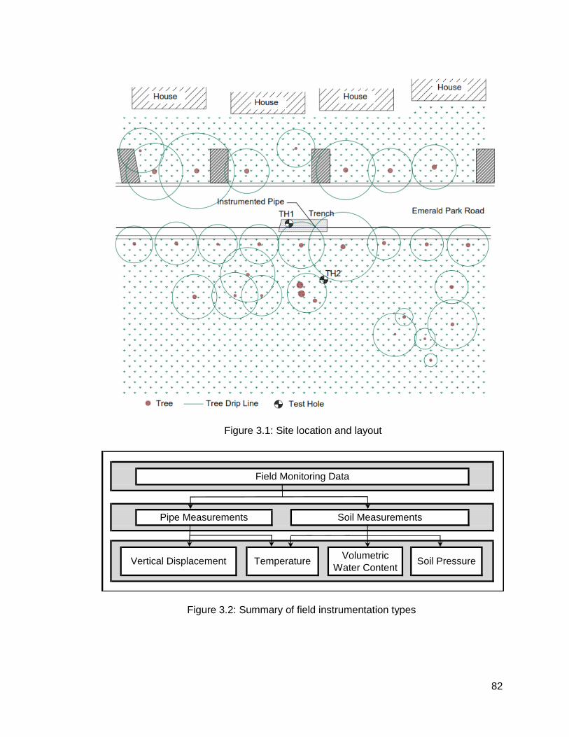
82
Figure 3.1: Site location and layout
Figure 3.2: Summary of field instrumentation types
Volumetric
Water Content
Soil MeasurementsPipe Measurements
Field Monitoring Data
Temperature Soil PressureVertical Displacement

83
Table 3.1: Dimensions and properties of the existing AC pipe section
Property Value
Nominal diameter (mm) 150
Outer diameter (mm) 183
Inside diameter (mm) 153
Length (m) 4
Elastic modulus (GPa) 20 – 25
Ultimate tensile strength (MPa) 25
Strain to failure (%) 0.1
Poisson’s ratio 0.3
Thermal coefficient (× 10–6/°C) 8.5
Table 3.2: Dimensions and properties of the Instrumented PVC pipe
Property Value
Nominal diameter (mm) 150
Outer diameter (mm) 175
Inside diameter (mm) 155
Length (m) 4
Elastic modulus (GPa) 2.8
Ultimate tensile strength (MPa) 48
Strain to failure (%) 10
Poisson’s ratio 0.42
Thermal coefficient (× 10–6/°C) 79

84
3.3 Instrumentation Details
Table 3.3 presents some of the necessary details of the sensors installed at the
site. Figure 3.3 presents a section layout showing the locations of the sensors that were
installed on site. A total of thirty (30) volumetric water content sensors (WCR) were
installed in the backfill and surrounding native soil to observe the moisture content
profiles. The WCR probes were calibrated for the native soil conditions (Hu et al., 2008).
Four pressure cells were placed in the vertical and horizontal directions to measure both
vertical and horizontal soil pressures. The pressure cells with a 350 kPa capacity were
installed in the trench backfill at a depth of about 170 mm above the top of the pipe.
Calibration curves for the pressure cells were provided by the manufacturer (Hu and
Lotfian, 2006). In addition, twelve (12) thermocouples were installed on the pipe exterior
surface; and thirty three (33) thermocouples were placed in the backfill and the native
soil surrounding the trench.
Three custom-built Geokon Model 4450 vibrating wire displacement transducers
were installed to measure the pipe displacements with time. The rod extensometers
were installed with one end of each extensometer being attached to the instrumented
pipe section, and the other end was installed in a test hole and anchored to the ground
at a depth of about 6.6 m below the ground surface. The test holes were backfilled with
bentonite plug to prevent water flow into the test holes. An automatic data acquisition
system was installed to collect and monitor pipe deformation, volumetric water content,
earth pressure, pipe displacements, and soil temperatures. The type of data acquisition
system used was manufactured by Campbell Scientific and the model was CR1000-55.
The data-logging equipment was kept in a metal instrumentation box in the field, and the
collection frequency was every hour.

85
Table 3.3: Summary of the main details of the instruments installed at the field site
Property Instrument Type Range (unit)
Accuracy (unit)
Pipe vertical displacement
Displacement (Custom-built 4450) (Geokon)
0 to 300 (mm) ± 0.1 (%)
Temperature Thermocouples (T type) (Veriteq Instruments)
-190 to + 350 (oC) ± 0.40 (°C)
Soil pressure Pressure cell (Model 4810X) (Geokon)
0 to 350 (kPa) ± 0.1 (%)
Soil volumetric water content
Water content reflectometer (CS616)(Campbell Scientific)
0 to 100 (%) ± 2.5 (%)
Figure 3.3: Schematic of the installed sensors layout at the field site

86
3.4 Climate Data
The climate data for the study area was retrieved from a nearby Environment
Canada meteorological station (Regina International Airport, Regina, Saskatchewan).
Figures 3.4 to 3.8 show the climate data including daily precipitation, air temperature,
wind speed, net radiation, and relative humidity covering a range from November 2005
to November 2007. The presented climate data was used as input for the numerical
modeling program. The total precipitation accounted for rainfall (primarily during the
summer) and snow (primarily during the winter). It is also to be noted that the historical
temperature data indicated that the monthly mean temperature is below 0 °C for 5
months from November to March every year.

87
Figure 3.4: Daily and cumulative precipitation at the field site
Figure 3.5: Daily air temperature at the field site
Nov-05 Feb-06 May-06 Aug-06 Nov-06 Feb-07 May-07 Aug-07 Nov-07
Date (mmm-yy)
0
10
20
30
40
Pre
cip
itation (
mm
)
0
200
400
600
800
1000
Cum
ula
tive P
recip
itation (
mm
)
Precipitation
Cumulative Precipitation
Nov-05 Feb-06 May-06 Aug-06 Nov-06 Feb-07 May-07 Aug-07 Nov-07
Date (mmm-yy)
-40
-20
0
20
40
Te
mpe
ratu
re (
oC
)

88
Figure 3.6: Daily wind speed at the field site
Figure 3.7: Daily net radiation at the field site
Dec-05 Mar-06 Jun-06 Sep-06 Dec-06 Mar-07 Jun-07 Sep-07
Date (mmm-yy)
0
20
40
60
Win
d S
pe
ed
(km
/hr)
Nov-05 Feb-06 May-06 Aug-06 Nov-06 Feb-07 May-07 Aug-07 Nov-07
Date (mmm-yy)
0
5
10
15
20
25
Ne
t R
ad
iation
(M
J/m
2/d
ay)
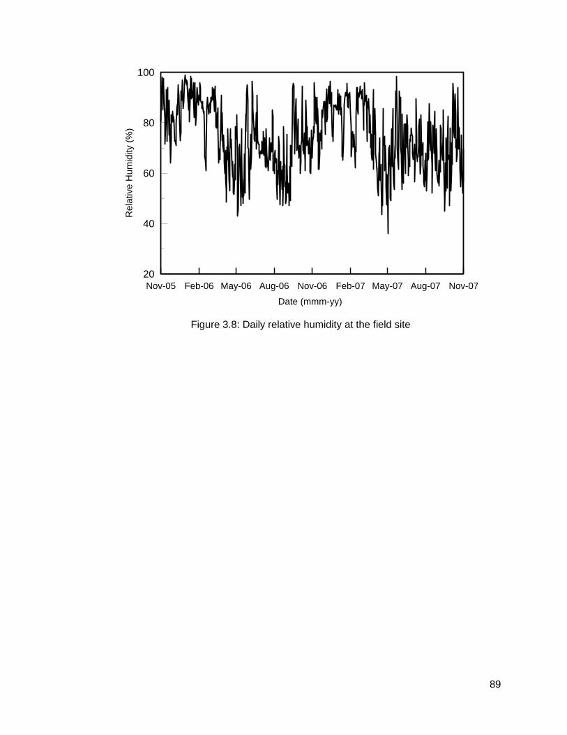
89
Figure 3.8: Daily relative humidity at the field site
Nov-05 Feb-06 May-06 Aug-06 Nov-06 Feb-07 May-07 Aug-07 Nov-07
Date (mmm-yy)
20
40
60
80
100
Re
lative
Hu
mid
ity (
%)

90
3.5 Backfill and Bedding Soils
The backfill and bedding soils in the trench consisted of mixed concrete (MC) and
sand, respectively. The grain size distribution curves for the bedding sand and mixed
concrete are shown in Figure 3.9. Clean sand was used as a bedding material below the
pipe. One sand lift was placed and compacted from the bottom of the trench to the
spring-line of the pipe (approximately 0.36 m deep). The trench was backfilled with MC
from the spring-line of the pipe up to the pavement base level.
The mixed concrete (MC) consisted of a blend of recycled crushed concrete and
sub-base gravel at a ratio of 2:1 by weight (Hu and Lotfian, 2006). The MC was installed,
in lifts of 150 mm, to the level of the underside of the pavement according to the
Construction Specifications of the City of Regina (Hu and Vu, 2011). The trench backfill
was compacted using a vibrating plate compactor. The water content and dry density
were measured in the field using a nuclear densometer.

91
Figure 3.9: Grain size distribution for backfill materials (sand and mixed concrete)
0.01 0.1 1 10 100
Particle Size (mm)
0
20
40
60
80
100
Perc
en
tag
e F
ine
r (%
)
Mixed Concrete
Sand

92
3.6 Soil Profile and Properties at the Field Site
Soils encountered in the study area were identified by two test holes before the
installation of the instrumented pipe section. The first test hole (TH1) was drilled in the
street, about 1.7 m west of the pipe. The second (TH2) was in the park, about 6 m east
of the pipe. Soils generally consisted of lacustrine clay which extended to a depth of
about 9.5. Clay till layer was encountered below the clay and extended to the bottom of
the test holes. Laboratory testing was reported for selected soil samples, including index
tests, soil-water characteristic curves, saturated hydraulic conductivity tests, swelling
tests, consolidation tests, and measurement of soil suction (Hu and Vu, 2011).
The upper soil layer was identified as highly plastic lacustrine clay (Regina clay)
that was typically silty, moist and stiff to very stiff. Figure 3.10 shows the water content
and dry unit weight profiles at the field site. The clay was also found to be over-
consolidated with an over-consolidation ratio of approximately 5.0. The measured
swelling pressure ranged from 500 to 550 kPa. The clay was also identified to exhibit
significant swelling and shrinkage characteristics upon wetting and drying.
The grain size distribution curve for both the top Regina clay and clay till samples
were plotted in Figure 3.11. Tables 3.4 and 3.5 show a summary of the key geotechnical
index properties for Regina clay and clay till soils. The grain size distribution curve
shows that the Regina clay consists of silt and clay maximum content (size less than 74
m) in the range of 98.7% - 99.9%. The liquid limit (LL), plastic limit (PL), and plasticity
index (PI) were measured to be in the range of (64 % - 94%), (23% - 35%), and (37% -
66%), respectively. The measured water content for the field samples ranged from 23%
to 35%. The soil specific gravity (Gs), average void ratio (e), and average dry unit weight
(yd) were found to be 2.73, 0.95, and 1540 kg/m3, respectively. The field matric suction
was found to be in the range of 700 kPa to 3000 kPa, and the approximated swelling
index (Cs) was measured to be approximately 0.09.

93
In general, the clay is considered non-plastic when it has a moisture content that is
less than the plastic limit (White, 1949). Therefore, the clay would likely be cracked or it
has a tendency to develop cracks with any reduction in its moisture content. Based on
the soil moisture content results, the upper two to three meters of the clay were found to
have a natural moisture content that was less than that of the lower clay layer. In
addition, the upper clay layer was also found to have an average moisture content that
was less than the plastic limit demonstrating that the clay was desiccated. (Hu and Vu,
2011) also illustrated that large surficial cracks, approximately 10 mm wide, were
observed in the study area.

94
Figure 3.10: Water content and dry unit weight profiles with depth at the field site
10 15 20 25 30 35 40
Water Content (%)
16
12
8
4
0
Dep
th (
m)
TH1
TH2
Clay
Clay Till
13 14 15 16 17 18 19
Dry Unit Weight (kN/m3)
16
12
8
4
0
Dep
th (
m)
TH1
TH2
Clay
Clay Till

95
Figure 3.11: Grain size distribution of Regina clay and clay till
0.001 0.01 0.1 1 10
Particle Size (mm)
20
40
60
80
100
Perc
en
tag
e F
ine
r (%
)
Regina Clay
Clay Till
Silt and clay content (74m)
- For Regina Clay = 99.9 (%)- For Clay Till = 95.8 (%)

96
Table 3.4: Geotechnical index properties of Regina clay
Soil Property (unit) Value
Specific gravity 2.73
Average dry density, yd (kg/m3) 1540
Moist unit weight, yw (kN/m3) 19.87
Natural water content, w (%) 23 – 35
Liquid limit, LL (%) 64 – 94
Plastic limit, PL (%) 23 – 34
Plastic index, PI (%) 37 – 66
Void ratio, e 0.95
Poisson’s ratio, (predicted) 0.33
Field suction-filter paper (kPa) 700 – 3000
Saturated hydraulic conductivity (m/s) 1.6 × 10⁻⁹ to 2.8 × 10⁻⁸
swelling index, Cs 0.09
Corrected swelling pressure (kPa) 500 – 550
Gravel content (≤62 mm) (%) 0.0 – 0.4
Sand content (≤5 mm) (%) 0.1 – 1.3
Silt and clay content (≤74 mm) (%) 98.7 – 99.9

97
Table 3.5: Geotechnical index properties of glacial clay till
Soil Property (unit) Value
Dry density, yd (kg/m3) 1900
Moist unit weight, yw (kN/m3) 21.2
Natural water content, w (%) 12 – 20
Liquid limit, LL (%) 38 – 44
Plastic limit, PL (%) 14 – 20
Plastic index, PI (%) 23 – 28
Field suction-filter paper (kPa) 2000
Gravel content (≤62 mm) (%) 0 – 3.6
Sand content (≤5 mm) (%) 4.2 – 31.8
Silt and clay content (≤74 mm) (%) 66.5 – 95.8

98
3.7 Unsaturated Soil Characteristics
Figure 3.12 also shows the soil-water characteristic curve (SWCC) of Regina clay
predicted using the laboratory measurements of soil suctions based on Fredlund and
Xing Fitting equation (Fredlund and Xing, 1994). The development of the SWCC for the
naturally deposited clay soil is discussed later in the thesis. The SWCC for the clay till
and backfill materials (sand and mixed concrete) were estimated based on the index
properties and the grain size distributions using the methods documented by (Fredlund
and Xing, 1994; Fredlund et al., 2002). Figures 3.13 and 3.14 show the soil-water
characteristic curve (SWCC) for clay till, sand and mixed concrete.
The measured saturated hydraulic conductivity of the clay ranged from 1.6 X 10⁻⁹
m/sec to 2.8 X 10⁻⁸ m/sec. The saturated hydraulic conductivity of the clay till, sand and
mixed concrete were estimated based on the grain size distribution, using Hazen’s
equation (Hazen, 1892), to be 1.0 X 10⁻⁸ m/sec, 2.30 X 10-05 m/sec and 7.50 X 10-06
m/sec, respectively. The unsaturated hydraulic conductivity functions for the native clay,
clay till and the backfill materials were estimated, using the Leong and Rahardjo
equation (Leong and Rahardjo, 1997), and based on the saturated hydraulic
conductivity. Hydraulic conductivity functions were plotted for Regina clay, clay till, sand,
and mixed concrete in Figures 3.15 and 3.16.

99
Figure 3.12: Soil water characteristic curve (SWCC) for Regina Clay
Figure 3.13: Soil water characteristic curve (SWCC) for clay till
0.1 1 10 100 1000 10000 100000 1000000
Matric Suction, (kPa)
0
0.1
0.2
0.3
0.4
0.5
0.6
0.7
Vo
lum
etr
ic W
ate
r C
on
ten
t, (
vo
l/vo
l)
Fredlund and Xing SWCC Fit
Laboratory Measurements
Saturation Suction = 0.1 kPa
Residual Volumetric Water Content, s= 0.12
Air Entry Value, AEV103.5 kPa
1 10 100 1000 10000 100000 1000000
Matric Suction, (kPa)
0
0.1
0.2
0.3
0.4
0.5
Vo
lum
etr
ic W
ate
r C
on
ten
t, (
vo
l/vo
l)
Fredlund and Xing SWCC Fit
Saturation Suction= 1 kPa
Air Entry Value, AEV63.4 kPa
Residual Volumetric Water Content, s= 0.19

100
Figure 3.14: Soil water characteristic curves (SWCCs) for the backfill materials
Figure 3.15: Hydraulic conductivity functions for Regina clay and clay till
0.1 1 10 100 1000 10000 100000 1000000
Matric Suction, (kPa)
0
0.1
0.2
0.3
0.4
Vo
lum
etr
ic W
ate
r C
on
ten
t, (
vo
l/vo
l)
Sand
Mixed Concrete
Saturation Suction = 0.1 kPa
Residual Volumetric Water Content, s
- For Sand = 0.05
- For Mixed Concrete = 0.17
Air Entry Value, AEV
- For Sand = 5 kPa
- For Mixed Concrete = 0.92 kPa
Fredlund and Xing SWCC Fit
0.1 1 10 100 1000 10000 100000 1000000
Matric Suction, (kPa)
1E-012
1E-011
1E-010
1E-009
1E-008
1E-007
Hyd
rau
lic C
on
du
ctivity,
k (
m/s
ec)
Regina Clay
Clay Till

101
Figure 3.16: Hydraulic conductivity functions for the backfill materials
0.1 1 10 100 1000 10000 100000 1000000
Matric Suction, (kPa)
1E-008
1E-007
1E-006
1E-005
0.0001
Hydra
ulic
Co
nd
uctivity,
k (
m/s
ec)
Sand
Mixed Concrete

102
3.8 Soil Moisture Field Data
Figure 3.17 shows the volumetric water content (VWC) measurements at three
levels 0.45 m, 2.92 m, and 4.0 m at the field site in the clay deposits surrounding the
pipe trench. As a general trend, for clays at low levels (2.92 m, and 4.0 m), had
experienced relatively small variations in volumetric water contents which were found to
be up to 5 %. The variation of volumetric water contents corresponded to the seasonal
variation in the climate conditions, without significant transits during rainfall or snowmelt
events. The clay soil at a higher level had noticeable variations in volumetric water
content which typically corresponded to the seasonal variation in the climate conditions
and the rainfall or snowmelt events. The volumetric water content at a depth of 0.45 m
was found to be as low as 15 % to as high as 36 %. The volumetric water content (VWC)
measurements were used to predict the variation in soil suction using the soil water
characteristic curve (SWCC) as showed in Figure 3.18. The pattern of the variations of
volumetric water contents was observed for the soil suction. The maximum and
minimum soil suction for the clay deposit at the two levels 2.92 m and 4.0 m were
estimated to be in the order of 1150 kPa and 480 kPa; however they were found to be in
the order of 36500 kPa and 2760 kPa at a depth of 0.45 m.

103
Figure 3.17: Volumetric water content in the clay deposit at various levels
Figure 3.18: Estimated soil suction in the clay deposit at various levels
Apr-06 Jun-06 Jul-06 Sep-06 Oct-06 Dec-06 Jan-07 Mar-07 Apr-07
Date (mmm-yy)
0
10
20
30
40
50
60
Vo
lum
etic W
ate
r C
on
ten
t, (
%)
0
10
20
30
40
Da
ily p
recip
itatio
n (
mm
)
Precipitation
Depth=0.45 m
Depth=2.92 m
Depth=4.0 m
Apr-06 Jun-06 Jul-06 Sep-06 Oct-06 Dec-06 Jan-07 Mar-07 Apr-07
Date (mm/dd/yy)
100
1000
10000
100000
Estim
ate
d S
uction
, (
kP
a)
0
5
10
15
20
25
Da
ily p
recip
ita
tio
n (
mm
)
Precipitation
Depth=0.45 m
Depth= 4.0 m
Depth=2.92 m

104
3.9 Air and Soil Temperatures
Figure 3.19 shows the air and ground temperatures collected in a 1-year period
from April 2006 to April 2007 following the pipe installation. The soil temperatures
experienced maximum and minimum peak temperatures corresponding to the air
temperature. The peak temperatures occurred at different time durations contingent on
the depth below the ground surface. In general, the shallower the depth, the earlier the
peak temperature occurred. At a depth of 0.45 m, the peak temperatures occurred at a
time that was close to the peak air temperature. However, there was a delay for the
maximum and minimum peak temperatures to occur at the pipe level. Detailed
discussions concerning the soil temperature with time are included later in the thesis.
3.10 Measured Pipe Displacements
The instrumented pipe displacement varied significantly throughout the
monitoring period. Figures 3.20 and 3.21 show the variation in pipe displacement with
time. The pipe experienced significant displacement peaks, in a 12-month period, a
relatively small one in the winter season and large ones in the spring/summer season.
Pipe displacements were also found to be different along the pipeline which were
attributable to the performance of the pipe end restraints. Overall, the increase in soil
pressure resulted in downward pipe displacements. It is anticipated that the decrease in
soil moisture content caused the soil to shrink, which in return, reduced the soil friction.
The soil pressure borne by the pipe would normally increase as a result of any reduction
in soil friction (Moser, 1990). Upward pipe displacements were also observed and were
closely correlated to seasonal variations in weather conditions.

105
Figure 3.19: Air and soil temperature observed at the field site
Nov-05 Feb-06 May-06 Aug-06 Nov-06 Feb-07 May-07 Aug-07 Nov-07
Date (mmm-yy)
-40
-20
0
20
40
Te
mpe
ratu
re (
OC
)
Depth = 0.45m
Depth = 1.0m
Air
Depth = 2.92m
Depth = 4.0m

106
Figure 3.20: Pipe displacements and soil pressures at the field site
Figure 3.21: Pipe displacements at the field site
-20
40
100
160
220
280
-5
0
5
10
Apr-06 Jul-06 Oct-06 Jan-07 Apr-07
So
il P
ressure
(kP
a)
Pip
e D
isp
lacem
ent (m
m)
Date (mmm-yy)
Vertical Pressure
Horizontal Pressure
Maximum Displacement
Average Displacement
0
10
20
30
40
-5
0
5
10
Apr-06 Jul-06 Oct-06 Jan-07 Apr-07
Daily
Pre
cip
itatio
n (m
m)
Pip
e D
isp
lacem
ent (m
m)
Date (mmm-yy)
Precipitation
Maximum Displacement
Average Displacement

107
CHAPTER 4: LOAD-DEFORMATION ANALYSIS UNDER DIFFERENT SOIL
AND PIPE CONDITIONS
4.1 Problem Statement
A technically sound design of buried pipes has to be based on the pipe
characteristics, internal and external loads, and surrounding conditions such as backfill
and side fill materials, and installation depth. The main objective of this study was to
investigate the influence of the most significant design parameters of buried pipes. A
numerical program was established and used to estimate the elastic deformations of a
soil-pipe system under different soil and loading conditions through real-life scenarios.
The finite element modeling approach was used to account for volume change effects,
soil layering, and displacement of the pipe relative to the soil. The model was validated
using previously developed empirical design equations. The numerical analysis was
performed in order to predict the elastic deformations occurring due to various backfill
materials around the pipes, native soils around the trench, and diverse applied loading
magnitudes.
4.2 Governing Equations
The soil-pipe system was modeled as an elastic continuum. The elastic continuum
solution for buried pipes can be represented by Equation (4.1) as suggested by (Klar et
al., 2004).
[PS](u) = (F) (4.1)
where;
[PS] is the stiffness matrix of the pipe,
(u) is the pipe displacement, and
(F) is the force vector representing the soil loading.
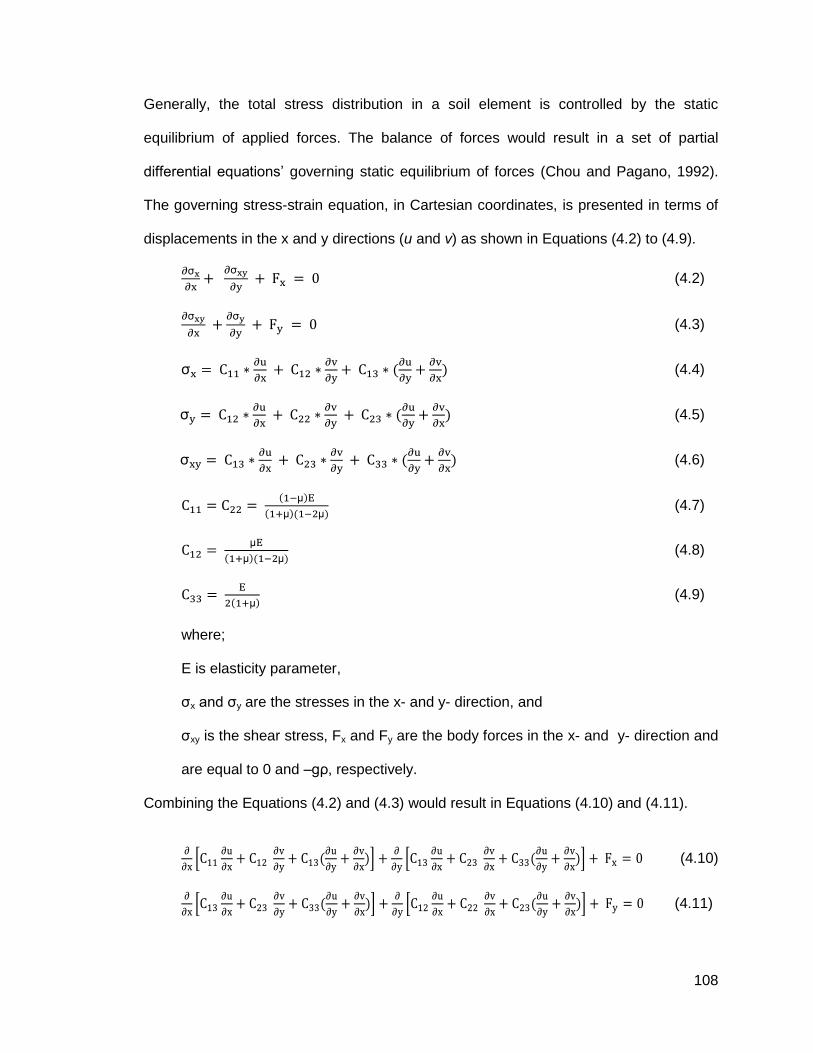
108
Generally, the total stress distribution in a soil element is controlled by the static
equilibrium of applied forces. The balance of forces would result in a set of partial
differential equations’ governing static equilibrium of forces (Chou and Pagano, 1992).
The governing stress-strain equation, in Cartesian coordinates, is presented in terms of
displacements in the x and y directions (u and v) as shown in Equations (4.2) to (4.9).
σ
σ
(4.2)
σ
σ
(4.3)
σ
(4.4)
σ
(4.5)
σ
(4.6)
(4.7)
(4.8)
(4.9)
where;
E is elasticity parameter,
σx and σy are the stresses in the x- and y- direction, and
σxy is the shear stress, Fx and Fy are the body forces in the x- and y- direction and
are equal to 0 and –gρ, respectively.
Combining the Equations (4.2) and (4.3) would result in Equations (4.10) and (4.11).
(4.10)
(4.11)

109
4.3 Modeling Overview, Geometry and Boundary Conditions
A two-dimensional soil-pipe model was developed to perform load-deformation
analysis as summarized in Figure 4.1. The analysis was conducted for a typical
underground pipe system that was under different soil and loading conditions. Figure 4.2
shows the model geometry and dimensions. The soil-pipe system was modeled under
strain conditions. The material used to fill the pipe trench was subdivided into three
different layers bedding, backfill, and cover. The natural soil surrounding the trench, the
soil in the trench, and the road pavement structures were modeled as separate layers. A
parametric study was initially conducted to evaluate the most significant design
parameters as reported in (Saadeldin et al., 2013b). The main features of the model can
be summarized as follows: (i) the soil and pipe materials were modeled in accordance
with the elastic continuum approach; (ii) live loads due to vehicular traffic were modeled
as a concentrated static load magnified by a dynamic amplification factor, and (iii) the
effect of variable water elevation was not modeled.
The appropriate boundary conditions were applied along the borders of the finite
element model. The bottom of the model was defined as a fixed boundary, where the
horizontal and vertical displacements were set equal to zero. However, the vertical sides
of the model had only a horizontal displacement equal to zero. Loads specified for the
analysis include the in-situ soil pressure in the soil profile and the assumed traffic loads.
Figure 4.3 presents the geometry and generated mesh of the model. The main input
parameters of the sensitivity analysis for the load-deformation analysis are summarized
in Table (4.1). The pipe was modeled as a 2D plane wall pipe with constant wall
thickness (t). The pipe used was a PVC pipe with (D/t) and initial Young’s modulus (Ep)
of 2.8 GPa. The road was modeled by a sub-pavement base of thickness equal to 0.25
m, and an asphalt layer of 0.1 m thickness.
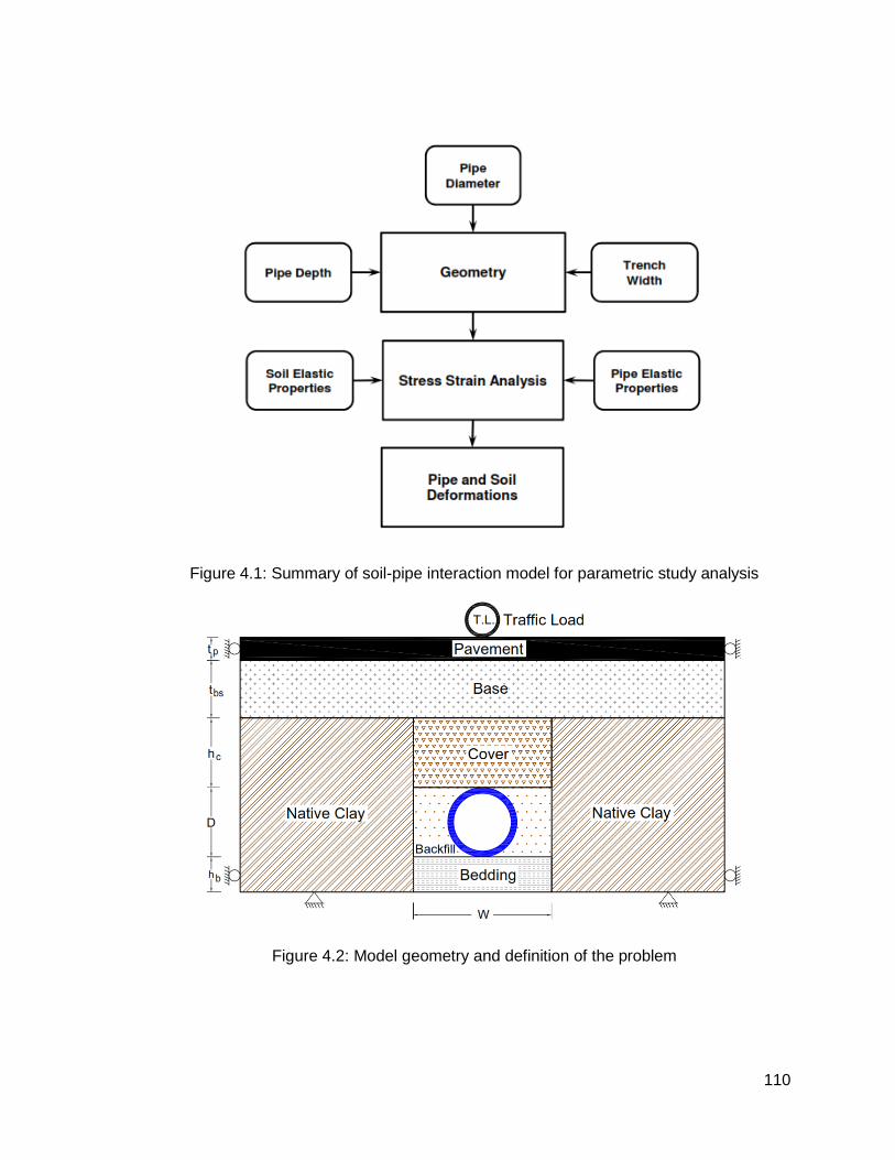
110
Figure 4.1: Summary of soil-pipe interaction model for parametric study analysis
Figure 4.2: Model geometry and definition of the problem

111
Figure 4.3: Generated mesh
(X and Y units are in meters)

112
Table 4.1: Summary of the main input parameters
Parameter (unit) Value
Pipe diameter to thickness ratio, D/t 10
Soil bedding thickness, hp (m) 0.15
Pavement thickness, tp (m) 0.1
Sub-base thickness, tbs (m) 0.25
Poisson’s ratio of pipe, p 0.4
Poisson’s ratio of clay, μs 0.3
Modulus of elasticity of clay, Es (kPa) 9500 - 47500
Modulus of elasticity of pipe, Ep (GPa) 2.8 - 280
Pipe diameter, D (m) 0.15 - 0.6
Cover thickness, hc (m) 0.3 - 2.0
Traffic load, T.L. (kN) 0.0 - 100

113
4.4 Numerical Modeling versus Analytical Results
Some of the model results, in the case of no applied surface traffic load and no
pavement structure, were compared with the results obtained by using Spangler’s
equation, illustrated earlier in this thesis. The soil load (wc) in Spangler’s equation was
obtained using the Marston load theory. In addition, as defined by Moser (1990), the
load coefficients (Cd) were determined to be 1.55 and 0.84 for a trench width of two and
six times the pipe diameter, respectively. It was observed that the results of the
numerical analysis matched the analytical results obtained by Spangler’s equation for
wider trench configuration. These findings and similarities led to higher deformations for
trenches of less width (i.e. twice the pipe diameter), as shown in Figure 4.4. It is
important to note that Spangler’s equation uses an individual value of the soil elastic
modulus to represent the backfill soil. However, the numerical simulation is capable of
fully considering the variation in elastic properties between the backfill soil and the native
soil surrounding the pipe trench.

114
Figure 4.4: Effect of the trench width on the maximum pipe deformations
10000 20000 30000 40000 50000
Modulus of Elasticity, Ef (kPa)
0
0.05
0.1
0.15
0.2
0.25
0.3
0.35
Pip
e D
efo
rmation,
D/D
(%
)
Native soil condition, Es=9500 kPaTrench
W
D
Ef
Es
12D
Spangler's equation
Modeling results
W= 2D
W= 6D
W= 6D
W= 2D

115
4.5 Pipe Deformations
The study analyzed the soil-structure interaction system under different soil and
pipe conditions. The field behavior of pipelines is significantly influenced by the trench
backfill, and the natural soil surrounding the trench. The surrounding backfill material
provides considerable support for underground flexible pipelines. It is well known that the
narrower the trench, the lighter the load applied to the pipe, and the pipe has to support
this load. However, in the case of flexible pipes, the pipe tends to rely heavily on the
surrounding soil to carry the applied loads. A flexible pipe principally derives its
resistance strength from the passive pressures induced by the relative movement of the
sides of the pipe against the surrounding soil (Moser, 1990).
Figure 4.5 shows the influence of soil elastic modulus on the surface displacement
under different surface traffic loads (T.L.) (i.e. 0 kN/m, 10 kN/m, 25 kN/m, 50 kN/m, 75
kN/m, and 100 kN/m). The increase in the soil elasticity, as an indicator of the soil
strength, resulted in reduced surface displacements and pipe deformations. It is a
practical and more efficient way of reducing the influence of earth loads on the pipe. The
higher strength of backfill reaction can be obtained by applying efficient compaction
conditions and using granular soils.
Figure 4.6 shows the influence of the soil cover thickness (hc) on pipe deformation
occurring under different surface traffic load magnitudes (i.e., 0 kN, 10 kN, 25 kN, 50 kN,
75 kN, and 100 kN). As a general trend, higher installation depths increased the effect of
soil load and decreased the impact of the surface load on underground pipelines.
However, pipe deformations were found not to increase monotonically with the increase
in soil cover under high surface loads.

116
Figure 4.5: Effect of soil modulus of elasticity on the overall soil surface displacement
Figure 4.6: Effect of soil cover height and loading conditions on pipe deformation
T.L.= 100 kN/m
T.L.= 75 kN/m
T.L.= 50 kN/m
T.L.= 25 kN/m
T.L.= 10 kN/m
10000 20000 30000 40000 50000
Soil Modulus of Elasticity, Es (kPa)
2
4
6
8
10
12
Su
rfa
ce
Dis
pla
ce
me
nt
(mm
)
Initial Condition, Es=9500 kPa
Ef/ Es=5
Ef/ Es=3
Ef/ Es=2
Ef/ Es=1.5
Ef/ Es=1.25
0 0.4 0.8 1.2 1.6 2
Soil Cover Height, hc (m)
0.1
0.2
0.3
0.4
0.5
0.6
0.7
Pip
e D
efo
rmation,
D/D
(%
)
Initial Condition, Es=9500 kPa
0 kN
10 kN
25 kN
50 kN
75 kN
100 kN

117
The performance of buried pipes was analyzed under different backfill material
conditions. As a general trend, higher backfill elasticity properties were found to make a
significant contribution to the behavior of flexible pipes. This response is a result of the
better confinement provided to the sides of the pipe with filling material that is stiffer than
the natural soil surrounding the trench. The performance of buried pipes was analyzed
under different backfill material conditions. Figure 4.7 shows the maximum pipe
deformations ( D/D) due to the increase in soil elasticity ratio between the backfill soil in
the trench and the native soil (Ef/Es). Two main cases were studied, including, trenches
with a width of two and six times the pipe diameter. When the backfill soil strength was
less than the native soil (Ef/Es < 1), the rate of increase in pipe deformation for the wide
trench was much higher than in the case of the narrow trench. Conversely, when the
backfill soil strength is greater than the native soil (Ef/Es > 1), the pipe deformation with a
wide trench was lower than in the case of a narrow trench.
In the event of a trench width of two times the pipe diameter, the resulting
reduction in the maximum pipe deformation was up to about 35% with an increase in soil
elasticity factor (Ef/Es) of 5. However, increasing (Ef/Es) to 5 in a trench width of six times
the pipe diameter resulted in a reduction in the pipe deformation up to about 60%.
Higher backfill strengths were found to make a considerable contribution to the behavior
of flexible pipes. This response is a result of the better confinement provided to the sides
of the pipe with filling material that is stiffer than the natural soil surrounding the trench.
These results confirm that flexible pipes mainly derive their ability to resist loads from the
lateral pressure of the soil along the sides of the pipes.
Pipe deformation increased with the decrease in pipe diameter and elastic
modulus as shown in Figure 4.8. It was generally observed that PVC pipes are subjected
to higher pipe deformations than rigid pipes due to their lower elastic modulus. The rate
118
of increase in pipe deformation with the decrease in pipe diameter was also found to be
different between 0.6 m to 0.3 m and 0.3 m to 0.15 m.
Field installation details and design criterion can be developed to determine the
optimized parameters as a function of the pipe characteristics (i.e., strength and
diameter), natural and backfill soil conditions, and surface loading conditions. Based on
the modeling results, it was observed that the pipe shares load with the soil beside it.
Loads are transferred through the compacted backfill material and the undisturbed
trench walls. Therefore, the trench width plays a role in controlling the net applied loads
on the pipe. It is essential to minimize the effect of trench width on the load reaching the
pipe. This cannot be achieved if the backfill material is not compacted. Therefore, it must
be recognized that adequate working space would then need to be provided. If working
space is insufficient, proper compaction for the backfill material beside and beneath the
pipe may not be achievable.

119
Figure 4.7: Effect of the backfill modulus of elasticity on pipe deformations
Figure 4.8: Effect of the soil cover thickness and loading conditions on pipe deformations
0 1 2 3 4 5
Modulus of Elasticity Ratio, Ef/Es
0
0.1
0.2
0.3
0.4
0.5
Pip
e D
efo
rmation,
D/D
(%
)
W= 2D
W = 6D
Native soil condition, Es=9500 kPa WTrench
D
Ef
Es
12D
0.15 0.2 0.25 0.3 0.35 0.4 0.45 0.5 0.55 0.6
Pipe Diameter, D (m)
0.2
0.3
0.4
0.5
0.6
0.7
Pip
e D
efo
rmation,
D/D
(%
)
Ep = 2.8 GPa
Ep = 28 GPa
Ep = 280 GPa
120
CHAPTER 5: PIPE RESPONSE TO RELATIVE SATURATION OF
SURROUNDING SOIL
5.1 Problem Statement
A large amount of water may enter soils during rainy seasons and result in
excessive soil heave whereas a significant reduction in water content during dry seasons
may result in settlement of soils as shown in Figure 5.1. Unsaturated soil surrounding
the pipes may, in return, swell and shrink which may change the loading on the pipes.
Pipeline design guidelines, such as those proposed by (Nyman, 1984), are typically
based on the assumption that the foundation soil is either fully saturated or dry. Until
now, the behavior of unsaturated soils on pipelines is not well understood. The modeling
technique adopted in Chapter 4 was modified to address the performance of a
hypothetical pipeline buried in an unsaturated clay soil.
The main objective of this study was to investigate the performance of small pipes
buried in unsaturated soil. The modeling analysis aimed to capture the pipe
displacements that occurred due to the change in soil suction associated with changes
in the soil moisture content. The soil suction was estimated based on field
measurements and was then used as an input for the model. The soil upward movement
was then simulated in order to draw conclusions regarding the behavior of pipes under
saturation of surrounding soils.
5.2 Governing Equations
The constitutive relationships for the modeling of unsaturated soil conditions were
developed as an extension of the saturated soil constitutive equations and utilized two
independent measures consisting of the total normal stress and soil suction. Soil
deformations occurred due to the change in total soil volume were then defined as the
summation of the normal strains in x- and y- directions (Fredlund and Morgenstern,

121
1976). The incremental elastic forms of these equations were provided in Equations
(5.1) to (5.8) (Fredlund and Vu, 2003). The main coefficients of volume change were
calculated as a function of the soil matric suction and net normal stress. The governing
stress-strain equations can be presented in terms of displacements in the x- and y-
directions (u and v). The stress-strain relation was assumed to be linear within each
stress and strain increment; however, the elasticity parameters, E and H, were allowed
to change in magnitude between increments.
(5.1)
(5.2)
(5.3)
(5.4)
(5.5)
(5.6)
(5.7)
(5.8)
where;
μs is the Poisson’s ratio for the soil,
Fx and Fy are x and y components of the body force vector,
E is the elasticity parameter as a function of the net normal stress,
H is the elasticity parameter as a function of the change in matric suction,
Cs and Cm are swelling indices obtained from net normal stress plane and matric
suction plane, respectively,

122
Ce, C11, C22, and C33 are the stiffness tensor components as defined by (Fredlund
and Gitirana Jr, 2005),
dσ is the net normal stress, and
d is the change in matric suction.
5.3 Modeling Overview, Geometry and Boundary Conditions
The proposed model was developed to solve the soil-structure interaction
equations under unsaturated soil conditions (Saadeldin et al., 2013b). Figure 5.2
describes the soil-displacement modeling approach for the analysis. Figure 5.3 presents
the geometry and boundary conditions used for the two-dimensional analysis. The soil
mass was divided into two main zones. The first zone (inactive zone) is covered with
pavement, which significantly reduces the infiltration of precipitation into the zone,
whereas the second zone (active zone) is directly subjected to various weather
conditions. The change in volumetric water content in the area studied was found to be
as low as 5%, as high as 20%, and corresponded well with the seasonal variations in
climate conditions.
Changes in soil suction subsequently occurred within the active soil depth. The
SWCC was estimated according to the unimodal Fredlund and Xing Fitting equation and
based on index properties, including water content (w), specific gravity (Gs), and dry unit
weight ( d). Soil suction profiles were predicted using the SWCC for the defined initial
and final soil moisture conditions. The soil under the pavement was assumed to have a
negligible matric suction change, a result of limited vertical moisture flows. Free
movement in the vertical direction was allowed at the top boundary and horizontal
movements of both the left and right sides were fixed. The lower boundary was fixed in
both directions. The boundary conditions of the pipelines were defined independently of
the side boundaries of the model to represent different end restraints.

123
The pipeline had a nominal diameter of 0.15 m, a total length of 6.5 m, and a
length of 4.0 m in the active zone. The pipe depth within the active zone was presented
by a relative depth ratio (DR) which was equal to the pipe depth divided by the total
active depth of the soil. The pipe elastic modulus and ultimate tensile strength were 2.8
GPa and 48 MPa, respectively. Figure 5.4 presents the adopted mathematical model of
the soil-pipe interaction. The field natural volumetric water content (θ) of Regina clay
was found to be around 40%. The field soil suction was measured to be around 2000
kPa. When water enters the soil, the soil suction gradually decreases. To account for
this decrease in soil suction for modeling purposes, a set of soil suction values (i.e. 1000
kPa, 500 kPa, 180 kPa, and 38 kPa) were modeled. This corresponds to an approximate
increase in volumetric water content (∆θ) of 5 %, 10%, 15%, and 20%. The soil suction
variation in the active zone was assumed to extend to the whole active depth. Some of
the main input parameters of the soil-pipe model are summarized in Table 5.1. The
modeling results were also obtained for a range of pipe conditions (i.e., elastic modulus,
depth, and end restraints).

124
Figure 5.1: Schematic diagram of the effect of dry and wet soil conditions on the pipe performance after (Rajeev et al., 2012)
Figure 5.2: Summary of the modeling procedure for displacement analysis
Input Processing
Material Index
PropertiesEstimated SWCC
Volume Change
IndicesInitial Suction State
Poisson's Ratio VWC Change, θ
Boundary Conditions Final Suction
Elasticity Modulus
Two Dimensional Soil-pipe Interaction Model
Displacement Data

125
Figure 5.3: Geometry for the two-dimensional soil-pipeline model
Figure 5.4: Theoretical model for the analysis of a buried pipe under unsaturated soil conditions

126
Table 5.1: Initial material parameters of the PVC pipe
Parameter Value
Nominal diameter, D (mm) 150
Total pipe length, L 6.5
Pipe length in active zone , X 4.0
Poisson’s ratio, µp 0.4
Elastic modulus, Es (GPa) 2.8
Ultimate tensile strength (MPa) 48
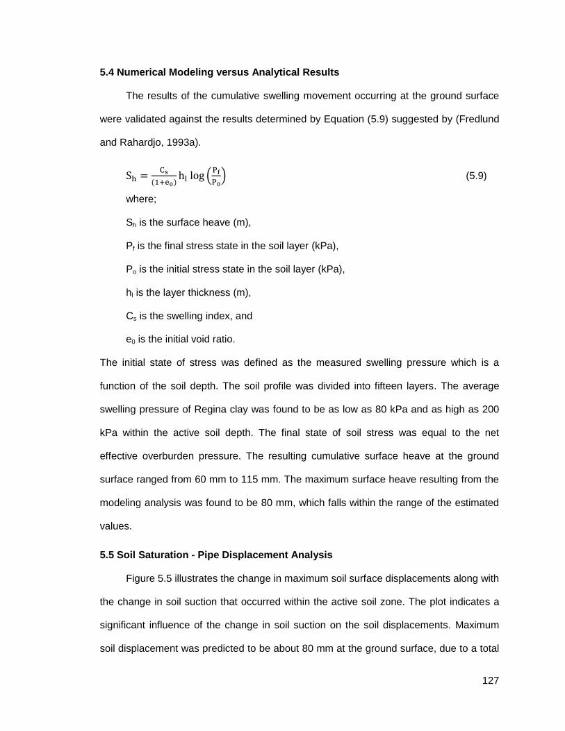
127
5.4 Numerical Modeling versus Analytical Results
The results of the cumulative swelling movement occurring at the ground surface
were validated against the results determined by Equation (5.9) suggested by (Fredlund
and Rahardjo, 1993a).
(5.9)
where;
Sh is the surface heave (m),
Pf is the final stress state in the soil layer (kPa),
Po is the initial stress state in the soil layer (kPa),
hl is the layer thickness (m),
Cs is the swelling index, and
e0 is the initial void ratio.
The initial state of stress was defined as the measured swelling pressure which is a
function of the soil depth. The soil profile was divided into fifteen layers. The average
swelling pressure of Regina clay was found to be as low as 80 kPa and as high as 200
kPa within the active soil depth. The final state of soil stress was equal to the net
effective overburden pressure. The resulting cumulative surface heave at the ground
surface ranged from 60 mm to 115 mm. The maximum surface heave resulting from the
modeling analysis was found to be 80 mm, which falls within the range of the estimated
values.
5.5 Soil Saturation - Pipe Displacement Analysis
Figure 5.5 illustrates the change in maximum soil surface displacements along with
the change in soil suction that occurred within the active soil zone. The plot indicates a
significant influence of the change in soil suction on the soil displacements. Maximum
soil displacement was predicted to be about 80 mm at the ground surface, due to a total

128
change in suction from 2000 kPa to 38 kPa. The figure also shows the maximum upward
displacements at the pipe level due to the same change in soil suction within the active
zone at a relative depth ratio (DR) of 0.9. The maximum pipe displacement was found to
be around 10 mm, at a depth of 2.7 m below the surface. The results of the upward soil
movement profiles can lead to an optimized pipe burial depth under the change in soil
suction and at the selected factor of safety. Similarly, avoiding the excessive fluctuation
in soil suction close to the area of the underground infrastructure may be an effective
way for minimizing soil movements and resulting displacement of underground
infrastructure.
Figure 5.6 presents the maximum pipe displacements predicted at the pipe level
for different pipe depth ratios of 0.5, 0.67, and 0.9. When the pipeline was installed at
shallower depth, it was subjected to higher displacement under the same variation in
water content and degree of saturation. The resulting pipe displacements increased
from 6% to 28% with the decrease of the relative depth ratio (DR) from 0.9 to 0.5. The
magnitude of upward soil movement was mainly affected by the change in soil elasticity
as a result of the increase in the total normal stress with depth.
Figures 5.7 and 5.8 show the normalized pipe displacement (pipe displacement/
pipe diameter, or d/D) profiles found at the pipe level along the pipeline length (X/L) at
different water content variations in the active zone. These two figures were obtained for
hinged and fixed end constraint conditions. In the case of hinged end restraints, the
maximum vertical displacement occurred at the left edge of the pipe in the active zone,
and it decreased along the length of the pipe. On the other hand, for fixed end restraints,
the maximum vertical displacement occurred around the approximate centre of the
active zone and decreased near the two edges of the pipeline.
The difference in the maximum normalized vertical displacement between the
hinged and fixed end restraint cases was found to be quite small (less than 0.2%) due to

129
the low modulus of elasticity for PVC pipes. For the studied cases, the maximum
normalized pipe displacement was found to be about 6%, corresponding to the relative
increase in volumetric water content, about 20% (approximately corresponds to the
change from the field condition to full saturation). The maximum pipe displacements
were approximately 2.1%, 3.7%, and 5.3%, with a relative increase in volumetric water
content of 5%, 10%, and 15% in the active zone, respectively.
In the case of significant variation environmental conditions applied on the ground
surface, burial depth was found to be a significant factor affecting the performance of
buried pipes. Burying pipelines should be completed deep enough to avoid significant
soil movements. The field ground surface conditions influence the amount of water
entered or lost from the soil structure and, therefore, it controls the burial depth. It is
important to take in consideration the actual condition of the ground surface in the
selection criteria of the burial depth of underground pipes. The right practice is to have
different burial depths with different surface conditions such as fully sealed surfaces
(concrete, pavement in good condition with no vegetation); semi-sealed surfaces (loose
fitting paving, loose fitting paving slabs), surfaces with vegetation trees and grass, and
unsealed surfaces.

130
Figure 5.5: Influence of the pipe burial depth on the pipe displacements
Figure 5.6: Maximum displacements versus normalized volumetric water content
Maximum Ground Displacement
Maximum Pipe Displacement
0 400 800 1200 1600 2000
Change in Soil Suction (kPa)
0
20
40
60
80
Dis
pla
cem
en
t (m
m) Initial suction = 2000 kPa
DR= 0.9
DR = 0.5
DR = 0.67
DR = 0.9
0 10 20 30 40 50
Normalized Volumetric Water Content, /i (%)
0
10
20
30
Maxim
um
Norm
aliz
ed
Pip
e D
isp
lace
men
t, d
/D (
%)
d/D = -0.005(/i)2 + 0.83(/i)
d/D = -0.003(/i)2+ 0.53(/i)
d/D = -0.001(/i)2 + 0.185(/i)

131
Figure 5.7: Pipe displacements due to the variation in soil moisture content under hinged end restraints
Figure 5.8: Pipe displacements due to the variation in the soil moisture content under fixed end restraints
0 0.2 0.4 0.6 0.8 1
Distance along the Pipe, X/L
-1
0
1
2
3
4
5
6
7
No
rma
lized
Pip
e D
ispla
ce
me
nt,
d/D
(%
)
Hinged-hinged Pipeline End Restrains
Active zone Inactive zone
= 20%
= 15%
= 10%
= 5%
Ep=2.8 GPa, DR=0.9
0 0.2 0.4 0.6 0.8 1
Distance along the Pipe, X/L
-1
0
1
2
3
4
5
6
7
No
rmaliz
ed
Pip
e D
ispla
ce
men
t, d
/D (
%)
Fixed-fixed Pipeline End Restrains
Active zone Inactive zone
= 20%
= 15%
= 10%
= 5%
Ep=2.8 GPa, DR=0.9

132
Figures 5.9 and 5.10 show the distribution of normalized pipe displacement along
the pipe for various properties of pipe materials. It was observed that the end restraints
of flexible pipes did not have an influence on the maximum displacement magnitudes of
the pipe (d/D). However it affected the distribution of displacement along the pipeline. On
the other hand, the end pipeline restraints showed a considerable effect on rigid pipes.
The maximum normalized pipe displacements were found to be around 6 % and 1.5 %
for hinged and fixed end restraints, respectively.

133
Figure 5.9: Pipe displacements in case of both hinged and fixed end restraints for a low elastic modulus magnitude (i.e. PVC pipe)
Figure 5.10: Pipe displacements in case of hinged and fixed end restraints for a high elastic modulus magnitude (i.e. steel pipe)
0 0.2 0.4 0.6 0.8 1
Distance along the Pipe, X/L
-1
0
1
2
3
4
5
6
7
No
rmaliz
ed
Pip
e D
ispla
ce
men
t, d
/D (
%) Fixed
Active zone Inactive zone
= 20 %
Ep=2.8 GPa, DR=0.9
Hinged
0 0.2 0.4 0.6 0.8 1
Distance along the Pipe, X/L
0
1
2
3
4
5
6
No
rma
lized
Pip
e D
isp
lace
men
t, d
/D (
%)
Fixed
Active zone Inactive zone
= 20 %
EP=280 GPa, DR=0.9
Hinged

134
CHAPTER 6: MATHEMATICAL FORMULATIONS OF SOIL-WATER
INTERACTION UNDER UNSATURATED SOIL CONDITIONS
6.1 Problem Statement
The mathematical formulation of unsaturated soil properties is necessary for the
computational modeling of water flow in soil deposits. As part of the formulation, it is
crucial to determine the soil water characteristic curve (SWCC) to identify the soil
response to transient water flow conditions. Transient water flow changes the stress
state in the soil structure, and consequently, the soil deforms in response to the changes
in the stress state and results in a new equilibrium state. The volume-mass constitutive
surfaces are the other key properties that provide an overall theoretical framework for
the soil state variables. The negative pore water pressure typically increases when a
load condition is being applied to an unsaturated soil structure. The consolidation
process may then take place when the excess pore water pressure is allowed to
dissipate and the soil volume will, subsequently, change with time. Therefore, for
unsaturated soils, the mechanical stress and pore water pressure should be coupled
together.
Unsaturated soils are often characterized by a variety of heterogeneities
(fractures/cracks) which affect water movement in soils (Novak et al., 2000). Infiltration
of precipitation and/or surface water into low-permeable soils (i.e. clays) is normally slow
(Novak et al., 2000). The presence of cracks increases the water flow into soil structure
and, in return, the soil water content. The depth of cracking is, therefore, a crucial
parameter that needs to be examined in order to understand the effects of desiccation
cracks. In the case of modeling saturated soils, the hydraulic conductivity can be
characterized by a lumped parameter because it contains relatively stable macropores
(Reynolds, 1993). Unsaturated cracked soils, however, cannot be modeled the same

135
way as saturated soils. Soil cracks are unstable and their geometry changes with time
depending upon the soil water content (Novak et al., 2000).
6.2 Methodology
In this chapter, a bimodal SWCC equation was developed for the native clay
deposit based on laboratory soil moisture-suction measurements. The proposed bimodal
SWCC equation was constructed by means of two distinct logistic power regression
models. A factor quantifying the change in the soil hydraulic conductivity was also used
to simulate the increase in the hydraulic conductivity of the cracked soil structure. In
addition, the hydraulic conductivity functions were developed for the cracked and un-
cracked soil layers. The constitutive surfaces were then established based on the
developed bimodal SWCC and representative consolidation test results. An unsaturated
seepage modeling analysis was also performed using the developed mathematical
framework. The model was utilized to simulate the application of net surface flux on a
soil column consisting of highly plastic clay over clay till. The sensitivity of the seepage
analysis, attributable to the variations in the SWCC and hydraulic characteristics, was
also demonstrated.
6.3 Fracture Depth Formulation
Morris et al. (1992) derived relationships between the cracking depth, depth to
ground water table, and surface suction as presented in Equation (6.1). The approach
assumed that the soil suction decreases linearly from the suction at the ground
surface (S0) to zero at the ground water table (dw) as presented in Equation (6.2).
The relationship also incorporated a coefficient representing the shear strength of the
soil as presented in Equations (6.3), (6.4) and (6.5).

136
(6.1)
–
(6.2)
(6.3)
(6.4)
(6.5)
Where;
is the cracking depth,
S is the suction,
S0 is the suction at the ground surface,
z is the depth below the ground surface,
is the distance from the ground surface to the ground water table,
is the compression modulus,
μ is the Poisson's ratio,
is the unit weight of soil,
is the coefficient for the angle of shearing resistance,
is the soil friction angle with respect to the total stress, and
is soil friction angle with respect to the soil suction.
Lau (1987) and Fredlund and Rahardjo (1993a) published a mathematical method
for determining the depth of cracking as a function of shear strength based on the
Rankine theory of lateral earth pressure as shown in Equation (6.6). The method
assumed that at rest, the coefficient earth pressure and the net horizontal stress were
equal to zero at the bottom of the soil crack. Figure 6.1 shows the mathematical model
for desiccation cracks and a typical soil suction profile presenting the negative pore-
water pressure as a linear function of distance above the groundwater table. The

137
equation is a function of the ground water depth, elasticity ratio, soil unit weight and
Poisson's ratio of soil. The relationship can generally be used to estimate the cracking
depth for a range of the elasticity ratio of soil.
μ
(6.6)
where;
is the depth of cracking,
/H is the elasticity parameters ratio. For an initially saturated clay, it ranges from
0.15 - 0.2 (Lau, 1987),
is the unit weight of water, and
is a variable used to permit the pore-water pressure to be represented as a
percentage of the hydrostatic profile.
Other variables were previously defined.

138
Figure 6.1: A typical desiccated soil profile and idealized matric suction profile, after
(Lau, 1987)

139
Values of the estimated cracking depth were determined using the two approaches
discussed above and presented in Equations (6.1) to (6.6). At the time of the field
investigation, there was no definite ground water table up to the explored depth of 16 m.
Due to the relatively granular and seepage nature of the clay till, the ground water depth
was then assumed to be either located at the maximum explored depth (16 m) or just
beneath the clay deposit (9.5m). The assumed ground water table levels are considered
reasonably representative of both highly wet conditions during rainy conditions and the
creation of a perched groundwater table within the clay till. Figures 6.2 to 6.4 show the
variation in estimated cracking depth at different ground water depths and different soil
conditions.
It was found that the linear elastic method resulted in higher estimated cracking
depths. Based on the analytical results, a cracking depth of up to 3 m can be expected
and can reasonably represents the field conditions as previously discussed. Based on
the results shown in Figure 6.2, a cracking depth of 3 m may be expected at a surface
suction of 100 kPa. In addition, based on the results shown in Figures 6.3 and 6.4, a
cracking depth of 3 m, may however, be expected at an elasticity ratio (E/H) of
approximately 0.15 and 0.11 for a ground water depth of 16 m and 9.5 m, respectively,
assuming that the hydrostatic profile factor is approximately 1.5.

140
Figure 6.2: Estimated cracking depth at different ground water depths (linear elastic theory)
Figure 6.3: Estimated cracking depth at a ground water depth of 9.5m (shear strength approach)
0 200 400 600 800 1000
Surface Soil Suction, So
0
4
8
12
16
Cra
ckin
g D
epth
, d
cr (m
)dw
= 16m
dw= 9m
1 1.2 1.4 1.6 1.8 2
Hydrostatic Profile Factor, fw
0
1
2
3
4
Cra
ckin
g D
epth
, d
cr (m
)
E/H = 0.2
E/H = 0.15
E/H = 0.1
E/H = 0.05
Ground Water Depth, dw= 9.5 m

141
Figure 6.4: Estimated cracking depth at a ground water depth of 16 m (shear strength approach)
1 1.2 1.4 1.6 1.8 2
Hydrostatic Profile Factor, fw
1
2
3
4
5
6
Cra
ckin
g D
epth
, d
cr (m
)
E/H = 0.2
E/H = 0.15
E/H = 0.1
E/H = 0.05
Ground Water Depth, dw= 16 m

142
6.4 Hydraulic Conductivity Formulation
The upper three meters of the clay layer were assigned a higher hydraulic
conductivity to simulate the effect of the seasonal development of desiccation cracks. A
hydraulic conductivity factor labeled (fcr) was assumed to stand for the increase in the
hydraulic conductivity due to the propagation of cracks. The hydraulic conductivity factor
was defined as the ratio between the hydraulic conductivity of the cracked soil structure
to the hydraulic conductivity of the natural soil (un-cracked) structure (fcr = kcr/kn). In view
of the fact that the crack development and distribution is a dynamic process and is
generally associated with the water infiltration/exfiltration processes. The factor was then
defined to be a function of the soil suction as a stress state that reflects the soil moisture
conditions.
The maximum increase in the hydraulic conductivity (a value represented by fmax)
is specified at the residual VWC and residual soil suction (Ψr) assuming that the cracks
are fully developed. However, the factor was assigned a value of 1 at completely
saturated condition (Ψsat). Using this definition, Equation 6.7 was incorporated into the
modeling program to simulate the final hydraulic conductivity of the top soil layer with
time.
Ψ Ψ
Ψ Ψ (6.7)
where;
is the hydraulic conductivity factor defining the ratio between cracked and un-
cracked soil condition,
is a variable used to represent the maximum hydraulic conductivity ratio
between cracked and un-cracked soil at an entirely dry condition,
Ψ is the soil suction,
Ψ is the soil suction corresponding to the residual VWC, and

143
Ψ is the soil suction corresponding to the saturated VWC.
6.5 Development of a Bimodal SWCC
Precise representation of the SWCC is essential for the seepage analysis of
saturated-unsaturated soil deposits. A bimodal SWCC was developed using the
measured data sets obtained from laboratory testing of the soil suction at different water
content levels. Figure 6.5 shows the measured data points for the field samples as two
sets, namely (1) and (2) that were obtained using the pressure plate and filter paper
methods as discussed in (Hu and Vu, 2011). The proposed equation of the bimodal
SWCC was developed using two distinct logistic regression models fitting the laboratory
data sets before and after a turning point. The turning point appeared at a soil suction of
100 kPa as shown in Figure 6.5. The developed equation and the corresponding fitting
parameters are included in Equation (6.8). It is important to mention that the presented
fitting equation was found to match a previous SWCC unimodal equation proposed by
(Gardner, 1958). However, the fitting parameters are predicted in the form of two sets,
in order to establish a bimodal curve. Figure 6.5 also shows the predicted SWCC using
the Fredlund and Xing fitting equation and based on the GSDC of the native clay.
θ θ
θ
θ
θ
θ
(6.8)
where;
θ is the volumetric water content (VWC) (vol/vol),
θt and t are the volumetric water content and soil suction at the turning point (0.53
and 100 kPa, respectively),
is the soil suction (1 ≤ ≤ 106 kPa),
θsat is the saturated volumetric water content (0.63) (vol/vol),

144
ai and bi are the curve fitting parameters for the first part of the curve (3.844, and
2.542, respectively), and
af and bf are the curve fitting parameters for the second part of the curve (3.56,
and 7.464, respectively).
The developed bimodal SWCC fitted well the laboratory data measurements and
showed two air entry values as initial and final values of 15 kPa and 200 kPa,
respectively. The bimodal SWCC was, however, positioned below the unimodal fit. Also,
with an increase in the soil suction, the difference between the unimodal and bimodal
SWCCs increased. This difference was considered as a good representation of the
divergence between the bases of developing each of these curves. Unimodal SWCCs
established based on the grain size distribution of the soil may take into account the
native formation of the particles. However, it is important to note that clay of dispersed
structure would result in a different soil water interaction behavior than that of fluctuated
structure even if both of them have the same grain size. The bimodal was, alternatively,
developed based on a reasonable range of measured VWC and soil suction values.
Therefore, it was able to better capture the structure of the clay. By comparing both the
unimodal and bimodal soil curves, it is clear that the bimodal curve, at the same soil
suction, shows greater water moisture reduction than the unimodal one.
A parametric study was conducted to determine the SWCC using different values
of fitting parameters. Figures 6.6 and 6.7 show the effect of change in fitting parameters
on the SWCC shape. It was noted that the fitting parameters can be used to plot a wide
range of variation in soil suction and VWC. It was also noted that the variation in the
parameter (a) did not result in a change in the slopes of the SWCC, and it controlled
more the position of the SWCC in relation to the best fit. However, the parameter (b) had
more control on the slope of the plotted SWCC. As shown in the figure, the bimodal
SWCC consisted of two SWCC functions that were superimposed to create one function

145
for the cracked soil as defined by (Durner, 1994). The two SWCC functions along with
their distinct parameters were developed representing the intact and cracked parts of the
soil. The bimodal SWCC was found to be a practical tool to simulate the soil as a dual-
porosity medium (Köhne et al., 2002). Using the developed bimodal SWCC, the soil
behavior can then be modeled as a combination of two materials averaged over the
whole soil volume demonstrating the change in the soil behavior caused by the soil
cracks (Fredlund et al., 2002).

146
Figure 6.5: Bimodal SWCC and laboratory suction measurements
Figure 6.6: SWCC shapes at different values for the fitting parameter (a)
1 10 100 1000 10000 100000 1000000
Matric Suction, (kPa)
0
0.1
0.2
0.3
0.4
0.5
0.6
0.7
Vo
lum
etr
ic W
ate
r C
on
ten
t, (
vo
l/vo
l)
Laboratory Measurements Set (1)
Laboratory Measurements Set (2)
Fredlund and Xing SWCC Unimodal Fit
Proposed SWCC Bimodal Equation Fit
Residual Water Content,s= 0.085
Initial Air Entry Value, AEVi
15 kPa
Final Air Entry Value, AEVf
200 kPa
1 10 100 1000 10000 100000 1000000
Matric Suction, (kPa)
0
0.1
0.2
0.3
0.4
0.5
0.6
0.7
Vo
lum
etr
ic W
ate
r C
on
ten
t, (
vo
l/vo
l)
Bimodal SWCC Equation
0.6a
0.8a
1.2aa

147
Figure 6.7: SWCC shapes at different values for the fitting parameter (b)
1 10 100 1000 10000 100000 1000000
Matric Suction, (kPa)
0
0.1
0.2
0.3
0.4
0.5
0.6
0.7
Vo
lum
etr
ic W
ate
r C
on
ten
t,
(vo
l/vo
l)
Bimodal SWCC Equation
0.6b
b1.2b
0.8b

148
6.6 Volume-mass Constitutive Relationships
The constitutive surfaces can typically be constructed using the relationships of the
void ratio, water content, and degree of saturation with the change in soil suction and net
normal stress. The unsaturated soil structure interaction under loading and unloading as
well as wetting and drying processes can be modeled using the volume-mass
constitutive surfaces. These constitutive surfaces define the primary soil state variables
(i.e., void ratio, water content and degree of saturation) as a function of the two
independent stress state variables (i.e. matric suction and net normal stress) forming 3D
surfaces. Using these constitutive surfaces, all soil state variables can be obtained over
the entire ranges of possible pore pressure and stress values. Matyas and Radhakrishna
(1968) recommended that the soil element can be graphically characterized as a point in
a system (i.e., a state point) where the coordinate axes stand for the state parameters, in
order that changes in the stress state can be defined as a state path. Fredlund and
Rahardjo (1993b) presented the main principles to construct 3D constitutive surfaces as
summarized below (Zhang, 2004):
(i) Void ratio versus net normal stress plot when the matric
suction is equal to zero, [e=f(σmean, = 0)],
(ii) Void ratio versus suction plot when the net normal
stress is equal to zero [e=f(σmean =0, )],
(iii) Water content versus net normal stress plot when the
matric suction is equal to zero, [w=f(σmean, = 0)],
(iv) Water content versus suction plot when net normal stress
equals zero, [w=f(σmean = 0, )],
(v) Degree of saturation versus mechanical stress plot when
the matric suction is equal to zero [S=f(σmean, = 0)], and

149
(vi) Degree of saturation versus matric suction plot when
net normal stress is equal to zero [S =f(σmean =0, )].
Two constitutive relationships are considered necessary for the two stress state
variables, one is a change in mechanical stress and the other is a change in matric
suction (Zhang, 2004). In order to define the constitutive relationships, the bimodal
SWCC was used to define the relationship between the matric suction and VWC. In
addition, previous laboratory measurements presented by Fredlund (1967) was used to
plot the relationship between the normalized VWC and mean normal stress. Figure 6.8
presents the relationship between the normalized VWC and mean normal stress as
defined in Equation (6.9). Figure 6.9 shows the different plots for the relationship
between the VWC and net normal stress using different values for the input fitting
parameters.
Likewise, previous laboratory measurements presented by Fredlund (1967) were
used to define the relationship between the normalized VWC and mean normal stress as
defined in Equation (6.10). This relationship was used to predict the degree of saturation
at different VWC levels. Figure 6.10 presents the relationship between the VWC and
degree of saturation. Figure 6.11 present the different shapes of the relationship at
different fitting parameters. Figures 6.12, 6.13, and 6.14 show the predicted volume-
mass constitutive surfaces. These constitutive surfaces were utilized to predict the
unsaturated soil properties of native clay. The plotted constitutive surfaces demonstrate
the change in the unsaturated soil properties for a range of the net normal stress and
soil suction. They incorporated the use of the bimodal SWCC that represents a good fit
with the laboratory measurements.

150
θ
θ σ σ σ
(6.9)
where;
σ σ and are fitting parameters, and σ is the net normal stress.
For Regina clay, best-fit curves were found with the following numerical values:
= 0.285593, 0.1815003, and -0.17729
θ
θ (6.10)
where;
and are fitting parameters,
is the degree of saturation, and
θ is the volumetric water content (VWC) (vol/vol).
For Regina clay, best-fit curves were found with the following numerical values:
b = 0.007576, c= 97.92621, and d = 2.17763

151
Figure 6.8: Normalized volumetric water content versus mean normal stress
1 10 100 1000
Mean Normal Stress, (kPa)
0
0.1
0.2
0.3
0.4
No
rmaliz
ed V
olu
me
tric
Wa
ter
Con
tent,
Obtained based on the Results of Fredlund (1967)
The Proposed Fitting Equation
= (a
+ b
log
mean)(
-1
d)
R2 = 0.999

152
Figure 6.9: Parametric analysis for normalized volumetric water content versus mean normal stress relationship
0
0.4
0.8
1.2
1.6
No
rma
lize
d V
olu
me
tric
Wate
r C
onte
nt,
Regina Clay (After Fredlund (1967))
0
1
2
3
No
rmaliz
ed V
olu
me
tric
Wa
ter
Con
tent,
1 10 100 1000
Mean Normal Stress, mean
(kPa)
0
0.2
0.4
0.6
No
rmaliz
ed V
olu
me
tric
Wa
ter
Con
tent,
b = 0.182, d = -0.177
a = 0.286, d = -0.177
a = 0.286, b
= 0.182
= (a
+ b
log
mean)(
-1
d)
a= 0.286
a= 0.1
a =
0.5
b= 0.182
b
= 0.1
b = 0
.3
d =
-0.1
77
d = -0
.1
d = -0
.3
R2 = 0.999

153
Figure 6.10: Degree of saturation versus volumetric water content
0 0.2 0.4 0.6 0.8 1
Volumetric Water Content, (vol/vol)
0
20
40
60
80
100
Deg
ree o
f S
atu
ration
, S
(%
)
Regina Clay (after Fredlund (1967))
The proposed equation
S = c d
b+d R2= 0.993

154
Figure 6.11: Parametric analysis for degree of saturation versus volumetric water content relationship
0
20
40
60
80
100
De
gre
e o
f S
atu
ratio
n,
S (
%)
Regina Clay (After Fredlund (1967))
0
20
40
60
80
100
De
gre
e o
f S
atu
ration
, S
(%
)
c = 100
c = 97.93
c = 95
0 0.2 0.4 0.6 0.8 1
Volumetric Water Content, (vol/vol)
0
20
40
60
80
100
De
gre
e o
f S
atu
ratio
n, S
(%
)
b =
0.02
b =
0.0
01
d =
2.1
8
d =
5
c = 97.93, d = 2.18
b = 0.008, d = 2.18
c = 97.93, b = 0.008
S = c d
b+d
b =
0.0
08
d = 1
R2= 0.993

155
Figure 6.12: Volumetric water content constitutive surfaces
Figure 6.13: Void ratio constitutive surfaces
110
1001000
0
0.1
0.2
0.3
0.4
0.5
0.6
0.7
Vo
lum
etr
ic W
ate
r C
on
ten
t,
(vo
l/v
ol)
0.6-0.7
0.5-0.6
0.4-0.5
0.3-0.4
0.2-0.3
0.1-0.2
0-0.1
1
10
100
1000
0
0.2
0.4
0.6
0.8
1
1.2
Vo
id R
atio
, e
1-1.2 0.8-1
0.6-0.8 0.4-0.6
0.2-0.4 0-0.2

156
Figure 6.14: Degree of saturation constitutive surfaces
110
1001000
0
20
40
60
80
100
De
gre
e o
f Sa
tura
tio
n,
S (%
)
80-100
60-80
40-60
20-40
0-20

157
6.7 Water Flow Mathematical Formulation
Above the ground water table, the pressure heads are negative, and the hydraulic
head can be determined indirectly through field measurements of the suction head or
negative pore-water pressure. As discussed earlier in this thesis, Fredlund and
Rahardjo (1993b) presented a general partial differential equation based on Richards’
equation for the transient moisture flow through saturated/unsaturated soils as illustrated
in Equation (6.11).
(6.11)
where;
h is the total head (m),
is the slope of the soil water characteristic curve, and
is the unit weight of water (kN/m3).
6.8 Parametric Study
6.8.1 General
A parametric study was performed to characterize the effect of the change in
unsaturated soil properties on the water seepage analysis for a soil column. The
numerical model validated the reliability of the mathematical framework and quantified
the effects of different boundary conditions. The modeling of soil moisture variation was
based on the governing partial differential equations of seepage through saturated-
unsaturated soils as discussed in the previous sections. The finite element modeling was
implemented using the commercial finite element program FlexPDE (PDE Solutions Inc.,
2014). The FlexPDE's model script was written based on the developed mathematical
framework and then the operations were executed to transform the description form of
the partial differential equations to a finite element model, run the analysis and produce
graphical demonstration of the results.

158
6.8.2 Methodology
The soil column consisted of a highly plastic clay (Regina clay) over clay till. The
width and height of the column were 3 m and 16 m, respectively. The finite element
mesh for the problem was generated by FlexPDE as presented in Figure 6.15. Cell sizes
were typically controlled by the spacing between explicit points in the domain boundary.
The developed initial mesh consisted of triangular finite elements with an average size of
0.4 m over the arbitrary two-dimensional problem domain.
The seepage analysis was performed using the following boundary conditions:
At the top of the column, a net flux was applied on the soil column. The
magnitude of the applied flux was assumed to be 0.75 mm/day, 1 mm/day, and 2
mm/day,
At the bottom of the column, net flux equaled zero,
The sides of the column had no applied flow boundary condition,
The highly plastic clay layer was divided into two layers, the upper layer
extended to a depth of (dcr), and the bottom clay layer extended to a depth of
9.5m, and
The initial VWC was assumed to be 0.3, 0.36, 0.25 for the top clay, bottom clay,
and clay till layers, respectively. The corresponding initial soil suction values
were then determined to be 2800 kPa, 1600 kPa, and 1400 kPa, respectively.
The seepage modeling results were obtained in terms of soil parameters such as VWC
and soil suction. The variation in these parameters as functions of both depth and time
were obtained at the following depths below the ground surface, 1.5 m (within the top
desiccated clay layer), 6.25 m (within the bottom clay layer), and 10 m (i.e., near the top
of the clay till layer).

159
Figure 6.15: Soil column configuration for the parametric study

160
6.8.3 Results and Discussion
A series of analyses using both unimodal and bimodal SWCCs were conducted
under a net surface flux of 1 mm/day and hydraulic conductivity factor of 1 as shown in
Figures 6.16 and 6.17. The pattern for the change in VWC was different, and roughly
followed the shape of the utilized SWCC characteristics. It is clear that the bimodal
SWCC resulted in a rapid reaction for the change in soil moisture conditions to the
applied net flux in comparison with the unimodal SWCC. The top clay layer approached
a full saturation condition in about five times the time required for the bimodal SWCC
model. The results suggest that the shape and characteristic of the SWCC have an
influence on the outcome of the seepage analysis and, therefore, the SWCC should be
formulated precisely to reflect the field conditions. Cracked soils were found to exhibit
bimodal behavior because of the pore space distribution discrepancy in the soil matrix
structure that is typically created by the cracks. The bimodal SWCC function resulted in
allowing greater infiltration and was considerably different from the unimodal one.
Therefore, it is clear that the use of bimodal SWCC provided a more practical method for
the simulation of the soil water interaction for highly plastic clays.
At a depth of 1.5 m and under a net surface flux of 1 mm/day and a maximum
cracking factor (fmax) of 1, 50, and 200, the variation in the resulting hydraulic
conductivity factor and the hydraulic conductivity of the top clay were plotted with time as
shown in Figures 6.18 and 6.19. The initial hydraulic conductivity of the clay was in the
order of 10-12 m/sec. The resulting initial hydraulic conductivity of the clay was in the
order of 10-10 m/sec (i.e., an increase of two orders of magnitude), and 10-11 m/sec (i.e.,
an increase of one order of magnitude) corresponding to fmax of 200 and 50, respectively.
The hydraulic conductivity was almost the same after approximately 235 days when the
soil approached near saturation condition.

161
Figure 6.16: Predicted suction profiles for Bimodal SWCC versus Unimodal SWCC
Figure 6.17: Predicted volumetric water content profiles for Bimodal SWCC versus Unimodal SWCC
0 500 1000 1500 2000 2500
Elapsed Time, days
0
1000
2000
3000
Matr
ic S
uctio
n, (
kP
a)
I = 1 mm/dayDepth = 1.5 m
B
A: Bimodal SWCCB: Unimodal SWCC
A
0 500 1000 1500 2000 2500
Elapsed Time, days
0.2
0.4
0.6
0.8
Vo
lum
etr
ic W
ate
r C
onte
nt,
(vol/vol)
I = 1 mm/dayDepth= 1.5 m
A
B
A: Bimodal SWCCB: Unimodal SWCC
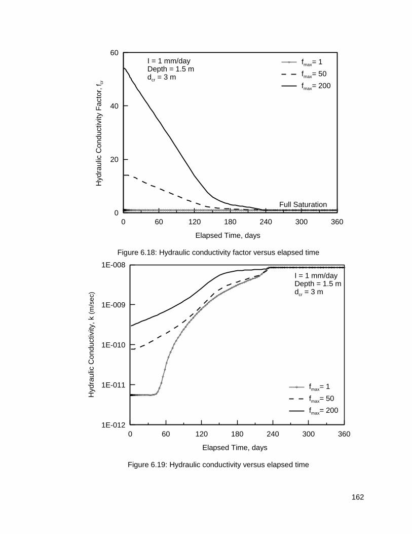
162
Figure 6.18: Hydraulic conductivity factor versus elapsed time
Figure 6.19: Hydraulic conductivity versus elapsed time
0 60 120 180 240 300 360
Elapsed Time, days
0
20
40
60
Hydra
ulic
Conductivity F
acto
r, f
cr
fmax= 1
fmax= 50
fmax= 200
Full Saturation
I = 1 mm/dayDepth = 1.5 mdcr = 3 m
0 60 120 180 240 300 360
Elapsed Time, days
1E-012
1E-011
1E-010
1E-009
1E-008
Hydra
ulic
Conductivity, k (
m/s
ec)
fmax= 1
fmax= 50
fmax= 200
I = 1 mm/dayDepth = 1.5 mdcr = 3 m

163
Figure 6.20 shows the variation in soil suction with the change in the hydraulic
conductivity of the clay. When the (fmax) increased from 50 to 200, the change in soil
suction was not as noticeable as the change from 1 to 50. In addition, the change in the
resulting VWC took less time to start with the increase in the hydraulic conductivity. This
overall behavior was reasonably able to model the dynamicity of the change of soil
hydraulic characteristics with the formation/ discontinuation of soil cracks.
The change in soil moisture was studied for different cases where the hydraulic
cracking factor was applied to different soil depths representing the increase in the depth
of the top desiccated clay layer. Using a maximum cracking factor (fmax) of 50, the
change in soil moisture characteristics were predicted for different cracking depths of 1
m, 2 m, and 3 m as shown in Figure 6.21. There were noticeable differences in the VWC
profiles with the increase in cracking depth. Due to the increase in the hydraulic
conductivity, the change in VWC started earlier and resulted in higher VWC magnitudes.
However, after a certain time period (approximately 50 days), increasing cracking depth
resulted in lower VWC magnitudes. This behavior reflected the effect of the change in
the seepage process of the cracked soil structure versus the un-cracked one. When the
soil is cracked to a certain depth, the water seepage is expected to be more rapid, and
water reaches a greater depth. However, the change in VWC at a certain depth would
take longer to reach saturation condition.
After approximately 140 days, the resulting VWC profile was almost the same with
the increase in cracking depth reflecting the small effect of soil cracking when the soil
reached near saturation condition. This behavior corresponded to the change in
hydraulic conductivity factor with time as described earlier. These results demonstrate
the significance of properly defining the depth of cracking in soil water interaction
analysis.

164
Figure 6.20: Predicted suction versus elapsed time at cracking factor magnitudes
Figure 6.21: Predicted volumetric water content versus elapsed time at different cracking depths
0 60 120 180 240
Elapsed Time, days
1
10
100
1000
Matr
ic S
uctio
n, (
kP
a)
fmax = 1
fmax = 50
fmax = 200
I = 1 mm/dayDepth = 1.5 mdcr = 3m
0 60 120 180 240 300 360
Elapsed Time, days
0.2
0.3
0.4
0.5
0.6
0.7
Vo
lum
etr
ic W
ate
r C
on
ten
t,
dcr= 0 m
dcr= 1 m
dcr= 2 m
dcr= 3 m
Full Saturation
fmax = 50, I = 1 mm/day
Depth = 1.5 m

165
Figures 6.22 and 6.23 show the variation in VWC and soil suction with time at
three different depths 1.5 m, 6.26 m, and 10 m below the surface. In general, there was
an increase in VWC with time as a result of the water seepage process. The VWC
gradually increased until it reached a constant value corresponding to the full saturation
condition. The change in VWC followed a bimodal pattern. A time delay for the start of
the change in VWC occurred and increased with the increase in depth reflecting the time
at which the soil water interaction started. Likewise, the time required to reach saturation
was different at each level.
Finally, the effect of the change in the applied surface flux was also investigated
as shown in Figures 6.24 and 6.25. Both VWC and soil suction gradually changed with
time and finally reached a constant value corresponding to those values at the full
saturation condition. There were differences in time at which the soil became saturated
for the different applied net fluxes. Increasing the magnitude of the applied flux resulted
in a rapid soil saturation progression. However, the variation in VWC and soil suction
followed almost the same pattern.

166
Figure 6.22: Predicted suction versus elapsed time at different depths
Figure 6.23: Predicted volumetric water content versus elapsed time at different depths
0 60 120 180 240 300 360
Elapsed Time, days
0
1000
2000
3000
Matr
ic S
uctio
n, (
kP
a)
Depth = 1.5 m
Depth = 6.25 m
Depth = 10 m
fmax = 1.0
I = 1 mm/daydcr = 3 m
0 60 120 180 240 300 360
Elapsed Time, days
0.2
0.3
0.4
0.5
0.6
0.7
Volu
me
tric
Wa
ter
Conte
nt, (
vol/vol)
Depth = 1.5 m
Depth = 6.25 m
Depth = 10 m
fmax = 1.0, I = 1 mm/day,
dcr = 3 m

167
Figure 6.24: Predicted volumetric water content versus elapsed time at different net surface flux magnitudes
Figure 6.25: Predicted suction versus elapsed time at different net surface flux magnitudes
0 60 120 180 240 300 360
Elapsed Time, days
0.2
0.3
0.4
0.5
0.6
0.7
Vo
lum
etr
ic W
ate
r C
onte
nt,
(vol/vol)
I = 2 mm/day
I = 1 mm/day
I = 0.75 mm/day
Full Saturation
fmax = 50
Depth = 1.5 mdcr = 3m
0 60 120 180 240 300 360
Elapsed Time, days
1
10
100
1000
Matr
ic S
uctio
n, (
kP
a)
I = 2 mm/day
I = 1 mm/day
I = 0.75 mm/day
fmax = 50
Depth = 1.5 mdcr = 3m

168
CHAPTER 7: SOIL-PIPE-ATMOSPHERE INTERACTION UNDER FIELD
CONDITIONS
7.1 Problem Statement
Predicting soil moisture content, soil suction, and temperature profiles is a key
element to study the field performance of underground pipelines. Developing a
framework to simulate real cases and incorporate more complex boundary conditions
and advanced unsaturated soil parameters is necessary. Desiccation cracks occur at
some stage due to the soil shrinkage during evapotranspiration processes (mainly, soil
water loss). The development of soil cracks influences the hydraulic conductivity and the
SWCC of the near-surface clay layers, and consequently, the moisture content changes
with time. Therefore, incorporating the development of soil cracks in the simulation of the
soil behavior is critical.
A key property that is vital for the implementation of unsaturated soil principles is
the soil water characteristic curve (SWCC). Bimodal SWCCs have not been heavily used
or verified in the modeling of the unsaturated soil deposits in many field applications, and
therefore, was used in this research study. Climatic conditions are other key factors of
the problem’s boundary conditions. However, data availability is a challenge constraining
not only the features of the modeling process but also the resulting predictive ability and
accuracy. Therefore, weather data from a nearby Environment Canada Meteorological
Station (ECMS) were analyzed for their applicability to the current study.
7.2 Methodology
The main objective of the proposed model was to investigate the response of a
150 mm PVC pipe buried in a highly plastic clay deposit under field conditions. A model
was established to incorporate the daily climatic conditions and to examine the effect of
the atmospheric conditions on the soil and pipe behavior. The required soil properties

169
and initial conditions for the model were determined from the laboratory results of the
collected samples from the field. To accurately model the field performance, advanced
interpretations were developed and validated to better simulate the development of
surface desiccation cracks. The factor quantifying the change in the soil hydraulic
conductivity, developed in this research, was used to model the increase in the hydraulic
conductivity of cracked soil structure compared to an un-cracked one. In addition, the
bimodal SWCC equation was utilized in this model to simulate the surficial highly plastic
clay layer surrounding the pipe trench.
The general processes and major steps of the numerical program are presented
in Figure 7.1. The program aimed to predict the displacement that occurred in the pipe
due to the change in climatic conditions with time. The model was established based on
a series of equations for heat and mass transfer in saturated-unsaturated soil structures
and a bimodal SWCC. The numerical model incorporated the simulation of the actual
evaporation of soil profile under field conditions. The prediction of final soil suction is the
connecting element between the two processes. The seepage analysis was established
to output time dependent suction changes influenced by the applied climatic conditions.
The stress-strain analysis used the suction data from the seepage analysis for its initial
and final conditions and then outputted the soil displacements. The entire analysis
utilized a general-purpose partial differential equation solver FlexPDE version 6 (PDE
Solutions Inc., 2014). The monitoring data of a section of an instrumented water pipe
buried in highly expansive native clay was also utilized. The field measurements were
utilized to develop the understanding of the soil-pipe interaction under field conditions,
and to quantify the effect of the variation of different soil-pipe parameters such as ground
surface conditions.

170
7.3 Geometry and Boundary Conditions
The modeling was undertaken using a two-dimensional model having the
atmospheric boundary condition at the top and no-flow boundary condition at the bottom
as well as left and right sides. Figure 7.2 presents the geometry and boundary conditions
used for the two-dimensional analysis. The pipe location and depth, pipe trench
dimensions and ground surface conditions were considered in accorance with the field
site conditions. Snow presence during the period between November and March was
assumed as total precipitation and applied right after the ground temperature rose to
above zero, representing the thawing process of the accumulated snow on the ground
surface. The surface boundary condition consisted of two zones to simulate the field site.
The first zone was covered with vegetation and, therefore, it was in full
interaction with the daily atmospheric conditions as well as the park watering during the
spring-summer season (from June to October). The park watering was assumed to be
applied twice a week with the amount of 1.81 mm per day in accordance with the field
site records. However, the second zone was covered with a pavement structure, which
reduced the soil-atmosphere interaction to some degree. Figure 7.3 shows the model
mesh for the analysis. Free movement in the vertical direction was allowed at the top
boundary and the horizontal movements of both left and right sides were fixed. The
lower boundary was fixed in both horizontal and vertical directions. The PVC pipe had a
nominal diameter of 0.15 m and was buried at a depth of 2.9 m below the ground
surface. Table 7.1 shows a summary of the key geotechnical index properties for the
native clay (Regina clay), the backfill (mixed concrete), and the pipe bedding (sand).
Table 7.2 shows a summary of the main parameters of the stress-strain modeling
analysis.

171
Figure 7.1: Soil-pipe-atmosphere modeling processes
Figure 7.2: Schematic diagram showing the field site conditions
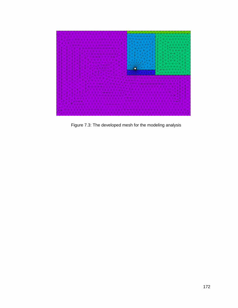
172
Figure 7.3: The developed mesh for the modeling analysis
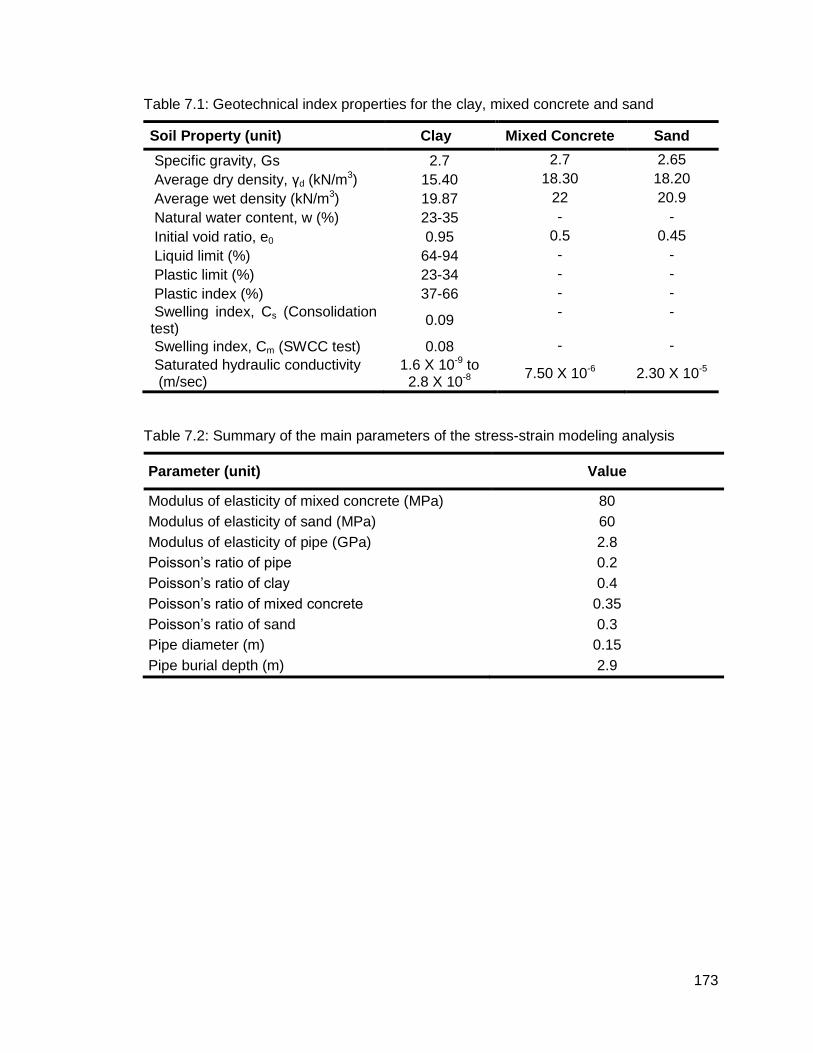
173
Table 7.1: Geotechnical index properties for the clay, mixed concrete and sand
Soil Property (unit) Clay Mixed Concrete Sand
Specific gravity, Gs 2.7 2.7 2.65
Average dry density, d (kN/m3) 15.40 18.30 18.20
Average wet density (kN/m3) 19.87 22 20.9
Natural water content, w (%) 23-35 - -
Initial void ratio, e0 0.95 0.5 0.45
Liquid limit (%) 64-94 - -
Plastic limit (%) 23-34 - -
Plastic index (%) 37-66 - -
Swelling index, Cs (Consolidation test)
0.09 - -
Swelling index, Cm (SWCC test) 0.08 - -
Saturated hydraulic conductivity (m/sec)
1.6 X 10⁻⁹ to 2.8 X 10⁻⁸
7.50 X 10⁻⁶ 2.30 X 10⁻⁵
Table 7.2: Summary of the main parameters of the stress-strain modeling analysis
Parameter (unit) Value
Modulus of elasticity of mixed concrete (MPa) 80
Modulus of elasticity of sand (MPa) 60
Modulus of elasticity of pipe (GPa) 2.8
Poisson’s ratio of pipe 0.2
Poisson’s ratio of clay 0.4
Poisson’s ratio of mixed concrete 0.35
Poisson’s ratio of sand 0.3
Pipe diameter (m) 0.15
Pipe burial depth (m) 2.9

174
7.4 Mathematical Formulation
7.4.1 Evapotranspiration Process
The term (Ep) was used to indicate the evapotranspiration flux from the soil surface
to the atmosphere. The analysis in this study was performed using the modified Penman
Equation (Penman, 1948) for actual evapotranspiration (Wilson et al., 1997; Wilson,
1990; Wilson et al., 1994). The potential evapotranspiration at the soil-atmosphere
boundary was calculated as shown in Equations (7.1) to (7.7).
(7.1)
(7.2)
(7.3)
(7.4)
(7.5)
(7.6)
(7.7)
where;
Ep is the evapotranspiration flux (m/day),
PE is the potential evapotranspiration (m/day),
RHa is the relative humidity at the soil surface,
is the air vapour pressure of air (mmHg),
is the air vapour pressure at the soil surface (mmHg),
is the saturation air vapour pressure (mmHg),
is the saturation air vapour pressure at the soil surface (mmHg),

175
is the slope determined from the saturation vapour pressure versus temperature
curve (mmHg/ºF) and can be determined as shown in Equation (7.6) (Zotarelli et
al., 2014),
QN is the net available radiant energy at the surface (m/day)(Gray, 1973);
is the psychrometer constant (0.27 mm Hg/ºF),
RHa is the air relative humidity,
Ta is the atmospheric air temperature,
Ua is the wind speed (m/day), and
Re is the net radiation.
7.4.2 Water Flow Equations
The transient moisture flow through saturated-unsaturated soil condition was
determined according to Equation (7.8) (Fredlund and Rahardjo, 1993b).
(7.8)
where;
h is the total pressure head,
kx is the hydraulic conductivity in x-direction,
ky is the hydraulic conductivity in y-direction,
is the slope of the soil water characteristic curve, and
is the unit weight of water.
The partial differential equation intended for conductive heat flow in soils was
identified according to Equation (7.9) (Pentland et al., 2001).

176
(7.9)
where;
λx and λy are the soil thermal conductivity in x- and y- direction,
T is the temperature,
c is the mass specific heat, and
ρ is the soil density.
The term cρ is designated to the volumetric specific heat capacity of the soil. The mass
specific heat (c) was assumed to be constant and estimated to be 1.2 x 10³ J/kg.K based
on the average of typical specific heat of soils (De Vries, 1963; List, 1966; Oke, 2002).
The thermal conductivity for the frozen and unfrozen backfill soil was estimated in
accordance with Equations (7.10) and (7.11) (Farouki, 1986; Kersten, 1949).
(7.10)
] (7.11)
Likewise, the thermal conductivity for the frozen and unfrozen native clay soil was
estimated in accordance with Equations (7.12) and (7.13) (Farouki, 1986; Kersten, 1949)
(7.12)
(7.13)
7.4.3 Stress-strain Equations
The governing nonlinear stress-strain equations are presented in terms of
displacements in the x- and y- direction (u and v). The incremental elastic forms of these
equations were provided in Equations (7.14) and (7.15) (Fredlund and Vu, 2003). The
incremental elastic forms of these equations were incorporated in Equations (7.16) and
(7.17) (Fredlund and Vu, 2003). The elasticity parameters were calculated using the
volume change indices and an assumed Poisson’s ratio.

177
(7.14)
(7.15)
(7.16)
(7.17)
where;
μs is the Poisson’s ratio for the soil,
Fx and Fy are x- and y- components of the body force vector,
E is the elasticity parameter as a function of the net normal stress,
H is the elasticity parameter as a function of the change in matric suction,
dσ is the net normal stress,
is the change in matric suction,
E is the elasticity parameter,
µ is Passions' ratio,
Cs and Cm are swelling indices obtained from net normal stress condition and
matric suction condition, respectively, and
Ce, C11, C22, and C33 are the stiffness tensor components as defined by (Fredlund
and Gitirana Jr, 2005).
7.5 Climate Data
The climate is a contributing factor to the seasonal variations in the moisture
content and temperature of the surficial soil layer. Air temperature and precipitation data
for the analyzed site were obtained from a nearby Environment Canada meteorological
station (Regina International Airport, Regina, Saskatchewan). The climate data,
including daily precipitation, air temperature, wind speed, net radiation, and relative
humidity were reported earlier among the field investigation details covering the time

178
span of field monitoring data and modeling duration. The total precipitation accounts for
rainfall and snow throughout the year.
7.6 Pavement Boundary Conditions
The pavement structure may experience different degrees of structural failures
(e.g. cracks) during its operations and, therefore, allows a percentage of the total surface
atmosphere applied flux to interact with the underlying material. The assumption of
having no applied flux because of the surface pavement structure is then invalid and is
not representative of the field conditions. In order to capture the variations in the VWC in
the trench backfill, a number of analyses have been completed to find out the amount of
the net flux transferred to the backfill material through the pavement structure. A
seepage ratio through the pavement (Rp) was defined as the ratio of the surface flux
below and above the pavement structure. The seepage ratio (Rp) was assigned different
values ranging from 0% to 100%. The resulting volumetric content was then compared
with the field measurements to predict the representative amount of applied flux through
the pavement structure.
7.7 Soil Temperature Analysis Results
Figures 7.4 and 7.5 compare the model outputs and the measured soil
temperature at depths of 0.45 m and 2.92 m, respectively, in the pipe trench below the
ground surface. The results show that the model captured the temperature variation for
the backfill material surrounding the pipe. The model outputs were in close agreement
with the field data near the ground surface. The model generated slightly lower
temperature values with a discrepancy of 6 °C to 9 °C. The backfill material experienced
periodic temperature changes due to the seasonal changes in air temperature. In the
soils above the pipe level, the temperature varied more in proximity to the ground
surface.

179
Soil temperatures experienced maximum and minimum peak temperatures
corresponding to the air temperature. The peak temperatures occurred at different time
durations contingent on the depth below the ground surface. In general, the shallower
the depth, the earlier the peak temperature occurred. At a depth of 0.45 m, the peak
temperatures occurred at a time that was close to the peak air temperature. However,
there was a delay of approximately 50 days for the maximum and minimum peak
temperatures to occur at the pipe level. Table 7.3 included a comparison of the change
in soil temperature from the field measurements and modeling results. The change in
soil temperature at the pipe level (2.92 m) was found to be around 13.8 oC and 13.7 oC
based on the modeling results and field measurements, respectively. This difference
increased significantly with the decrease in depth and reached approximately 42.1 oC
and 36.4 oC at a depth of 0.45 m, based on modeling results and field measurements,
respectively.

180
Figure 7.4: Soil temperature versus time in the pipe trench
Figure 7.5: Soil temperature versus time at a depth of 2.92 m in the pipe trench
Nov-05 Feb-06 May-06 Aug-06 Nov-06 Feb-07 May-07 Aug-07 Nov-07
Date (mmm-yy)
-40
-20
0
20
40
Te
mpera
ture
(OC
)
Air
Field Measuremets (0.45m)
Modelling Results (0.45 m)
Nov-05 Feb-06 May-06 Aug-06 Nov-06 Feb-07 May-07 Aug-07 Nov-07
Date (mmm-yy)
-40
-20
0
20
40
Te
mpe
ratu
re (
OC
)
Air
Field Measuremets (2.92 m)
Modelling Results (2.92m)

181
Table 7.3: Summary of the modeling results for the pipe trench for the period from April 2006 to April 2007
Parameter Depth
(m) Field Modeling
Soil Temperature Change, T (oC)
0.45 From -9.7 to 26.7
(36.4)
From -18.7 to 23.4
(42.1)
2.92 From 3.6 to 17.3
(13.7) From 5.4 to 19.2
(13.8)

182
7.8 Soil Moisture Analysis Results
The change in soil moisture due to the change in climatic conditions was modeled
over a 365-day period, between the 25th of April, 2006 and the 25th of April, 2007, for the
native clay and the backfill material. Figure 7.6 shows the variation in the VWC and
suction for the native clay versus depth with time obtained from the numerical modeling
analysis. The variation in VWC reflected well the seasonal variations in the climatic
conditions and the rainfall events. Soil layers close to the ground surface were highly
affected by the surface atmosphere conditions. The bimodal SWCC provided the model
with a good capability to capture the variation in the moisture content of the top clay
layer.
As a general trend, the VWC and soil suction varied considerably with time within
the upper two to three meters. It was clear that higher fluctuations in moisture content
occurred near the ground surface and diminished with depth. Figure 7.7 shows the
variation in VWC of the native clay deposits surrounding the pipe trench at a depth of
0.45 m from the field investigation and the numerical modeling analysis. The maximum
change in VWC was predicted to be in the order of 20.5% versus 17% from the field
measurements as summarized in Table 7.4. However, the change in VWC dropped
substantially with depth. The change in VWC at a depth of 2.92 m was predicted to be
5.5 % compared to 6 % based on the field measurements. However, the change in VWC
at a depth of 4 m was predicted to be 5 % compared to 4.5 % based on the field
measurements.
It was found that the numerical modeling results were in close agreement with field
measurements for unfrozen soil conditions (i.e. between April and November). Since the
moisture sensors in the field were not capable of measuring reliable volumetric water
contents readings during frozen soil conditions, the corresponding field measurements
have not been included. The climate data obtained from Environment Canada were

183
found to be adequate for the modeling of the soil moisture change in the field. Freezing
temperatures and snow falling started mid-November and continued as winter advanced.
Therefore, the sudden increase in the predicted VWC following the winter reflected the
thawing process of accumulated snow on the ground.
Figure 7.8 shows the effect of increasing the applied flux on the backfill in the pipe
trench. The net applied flux corresponds to full contact between the ground and the
atmosphere. The change in VWC of the backfill was predicted under different variations
in the applied surface flux as described earlier in this paper. The effect of the applied flux
decreased with the increase in soil depth. A normalized change in the VWC of more than
50% was predicted assuming that the full atmospheric induced net flux was applied to
the backfill material. Figure 7.9 shows the VWC of the backfill material at a depth of 0.45
m below the ground surface. Although the pipe trench was covered with a pavement
structure in the field, the backfill experienced changes in moisture content with time.
Table 4 shows the modeling results and field measurements for the change in VWC for
the backfill material at a depth of 0.45 m. The change in the VWC was measured in the
field to be approximately 13% at a depth of 0.45 m. It was, however, predicted that a
change of 14 % in the case of 30 % of the net atmosphere flux was applied on the pipe
trench.
In accordance with the modeling results and the field measurements, 30% of the
net flux was found to get through the pavement structure and interacted with the
underlying backfill material. In this study, the backfill material consisted of non-expansive
soil and, therefore, the variation in the soil moisture content did not result in additional
soil volume change. However, soil movements are still expected due to the swell-shrink
behavior of the clay surrounding the trench.

184
Figure 7.6: VWC and suction profiles at various levels for the native clay
Figure 7.7: VWC at a depth of 0.45 m versus time for the native clay
0 10 20 30 40 50
Volumetric Water Content, (%)
6
5
4
3
2
1
0
De
pth
(m
)
100 1000 10000 100000
Suction, (kPa)
6
5
4
3
2
1
0
10 Days (May, 5th)
45 Days (June, 10th)
120 Days (Aug., 25th)
150 Days (Sep., 25th)
330 Days (March, 25th)
Apr-06 Jun-06 Jul-06 Sep-06 Oct-06 Dec-06 Jan-07 Mar-07 Apr-07
Date (mmm-yy)
0
10
20
30
40
50
Vo
lum
etr
ic W
ate
r C
on
ten
t,
(%
)
Modelling Results (0.45 m)
Field Measurements
Precipitation
0
10
20
30
Pre
cip
ita
tio
n (
mm
)

185
Table 7.4: VWC change of the native clay for the period from 25th April 2006 to 25th April 2007
Depth (m) VWC Change, Δθ (%)
Field Modeling
0.45 17 20.5
2.92 6 5.5
4.0 5 4.5

186
Figure 7.8: Volumetric water content change in the pipe trench
Figure 7.9: Volumetric water content versus time in the pipe trench
0 20 40 6010 30 50
Normalized Volumetric Water Content, /o (%)
3
2.5
2
1.5
1
0.5
De
pth
(m
)
Fluxp = Assumed Net flux
through the pavement cracks = Rp * Net Atmospheric Flux
Rp= 100%
R p= 40%
R p= 30%
R p=
20%
Rp
= 1
0%
o = Initial VWC
Apr-06 Jun-06 Jul-06 Sep-06 Oct-06 Dec-06 Jan-07 Mar-07 Apr-07
Date (mmm-yy)
0
10
20
30
40
Volu
me
tric
Wa
ter
Co
nte
nt,
(%
)
Modelling Results (0.45 m)
Field Measurements (0.45 m)
0
10
20
30
Pre
cip
ita
tio
n (
mm
)

187
7.9 Soil and Pipe Displacements with Time
Figure 7.10 shows the variation in pipe displacements obtained from the field
monitoring program and the modeling analysis. The field data are the average of
displacements recorded at three locations along the pipe. The total pipe displacements
obtained from the modeling analysis were determined considering the swell-shrink
displacements for the native material surrounding the trench and the change in the net
normal stress of the backfill. It is clear that pipe displacements varied with time due to
the change in climatic conditions. Figure 7.11 shows the daily vertical displacements
predicted at the ground surface for the clay surrounding the trench and covered with
surface vegetation. The soil displacements corresponded to the precipitation and
evaporation events. Abrupt displacements up to 7.5 mm per day occurred at the ground
surface due to the change in the moisture content.
Although the pipe trench was backfilled with a non-expansive material to 3.0 m
below the ground surface and covered with a pavement structure, the pipe experienced
fluctuating movements due to the native clay surrounding the trench. The average pipe
displacement was measured in the field to vary from -2.3 mm to 5.5 mm. The predicted
pipe displacements changed from -1.8 mm to 3.1 mm. The difference between the
modeling results and the field measurements may be attributed to the fact that the
freeze-thaw analysis was not incorporated. It is also to be noted that the magnitude of
the pipe displacement is expected to be more if the pipe was to be backfilled with the
native clay material.

188
Figure 7.10: Pipe displacements versus time
Figure 7.11: Daily ground displacements (native clay)
May-06 Jun-06 Jul-06 Aug-06 Sep-06 Oct-06
Date (mmm-yy)
-10
-5
0
5
10
15
To
tal D
isp
lace
men
t (m
m)
Modelling Results
Field Measurements (Average Records along the Pipe)
0
4
8
12
16
20
Pre
cip
ita
tio
n (
mm
)
Apr-06 Jul-06 Oct-06 Jan-07 Apr-07Jun-06 Sep-06 Dec-06 Mar-07
Date (mmm-yy)
-5
-4
-3
-2
-1
0
1
2
3
4
5
6
7
8
Da
ily S
we
ll S
hri
nk D
isp
lace
me
nt
(mm
)
0
10
20
30
Pre
cip
ita
tio
n (
mm
)
Modelling Results (at the Ground Surface)

189
CHAPTER 8: SUMMARY, CONCLUSION AND FUTURE WORK
This chapter summarizes the main findings of this research study, including
engineering significance of the research, field observations, related technical
interpretations, and the results of the numerical modeling analysis.
8.1 Engineering Significance and Applications
The elevated annual breakage rates of buried pipes, especially small diameter
pipes, are a significant problem in arid and semi-arid regions, worldwide. Historical pipe
breakage rate records and field observations indicated that the pipe failure is strongly
correlated with ground movements and seasonal variation in climatic conditions. The
understanding of the correlation between pipe behavior and the most critical geo-
environmental conditions (i.e., soil moisture changes) is well developed. Finite element
methods can be used effectively to analyze this type of problems. The number of studies
on the behavior and performance of pipes under various weather conditions is still quite
limited. Consequently, the aim of this research was to enhance the current knowledge by
studying the performance of buried pipes under different field geo-environmental
conditions and the effects due to changes in unsaturated soil conditions. A better
understanding of unsaturated clays and pipe interactions can ultimately help reduce the
rate of buried pipe breakages.
8.2 Summary of Results
8.2.1 Field Investigation
Field monitoring data of the underground water main and surrounding soil provided
an understanding of the effect of soil on the behavior of buried pipes. It was found that
the soil and pipe behavior was influenced by the seasonal changes and correlated well
with the changes in the local meteorological conditions. The soil temperature, volumetric

190
water content (VWC), and suction were good indicators of the changes in the soil
behavior with the time throughout the year. The general pattern of variation in soil
temperatures was affected by air temperature and the depth below ground surface. The
volumetric water content of the backfill and the surrounding native soils at shallow
depths showed significant variations with respect to extreme weather events, especially
late March to early April as a representation of snowmelt event, and from May to June as
a representative of rainfall events. The effect of the seasonal variation decreased with
depth below ground surface.
As a general trend, clays at the pipe level of approximately 2.92 m, experienced
relatively small variations in volumetric water contents (VWCs), and were found to be in
the range of ± 5 %. The clay soil at a higher level, near the ground surface, had
prominent variations of VWC which corresponded well to the seasonal variation in the
climate conditions and the rainfall or snowmelt events. The change in VWC was found to
reach as high as 20 % at a depth of approximately 0.5 m below the ground surface. The
observations also confirmed that the wet-dry seasonal events can induce significant
displacements on the pipes. Theses displacements magnitude varied along the pipeline.
8.2.2 Load-deformation Analysis
The finite element modeling approach was established using the elastic continuum
theory. The soil-pipe system was considered as an elastic continuum with the
consideration of volume change effects, soil layering, and displacement of the pipe
relative to the soil. The performance evaluation study of the soil-pipe interaction included
the identification and modeling of a typical buried pipeline arrangement. The modeling
approach provided comparable results of maximum pipe deformations with the empirical
design equation (Spangler’s Equation). The key results of this performance evaluation
model can be summarized as follows:

191
The geometric configuration of the pipe trench, including the cover height
and trench width, significantly influenced the overall deformations of the soil-
pipe system. Increased trench width along with enhanced soil conditions
were found to provide more lateral support when the flexible pipe deforms.
The effect of the field configuration, such as the trench width, in the
calculation of pipe deformations, was found to be essential for capturing the
pipe deformations under field conditions.
Flexible pipes are subjected to higher deformations due to their low stiffness.
Pipe deformation was found to decrease with the increase in pipe diameter,
and elastic modulus of backfill materials. This effect is a result of the
improved confinement provided for the sides of the pipe.
8.2.3 Pipe Response to Unsaturated Soil Conditions
The behavior of a buried pipe in unsaturated clay soil was modeled under
saturation of the surrounding active layer. The adopted approach, through simulations of
possible scenarios, provided better understanding of the field behavior of underground
pipes. The pipe response was found to depend on the pipe depth, stiffness, and end
restraints. The main results of this model can be summarized as follows:
An increase in soil water content, corresponding to a decrease in soil suction,
resulted in significant upward displacements. The pipe displacements were highly
influenced by pipe burial depth. The upward movements of pipelines can be
notably reduced by a slight increase in burial depth.
For the case study dealing with a pipe buried at a depth of 2.7 m (a relative depth
ratio (DR) of 0.9 within the active soil zone):
o Maximum soil displacements at the ground and pipeline level were predicted
to be about 80 mm, and 10 mm, respectively. This was a result of a total

192
change in volumetric water content from 20% (close to the field condition) to
60% (close to the full saturation condition).
o Maximum pipe displacements of 2.1%, 3.7%, 5.3%, and 6.0% were reported
as results of the relative increase in volumetric water content of 5%, 10%,
15%, and 20%, respectively.
The end restraints of an underground flexible pipe (PVC pipe) affected the
distribution of displacement along the pipeline but had a minimal influence on the
maximum pipe displacement magnitude. However, the end restraints of an
underground rigid pipe (i.e. steel pipe) affected the distribution and magnitude of
displacement along the pipeline.
In case of fixed end restraints and under the same change in moisture content of
the soil, the maximum upward displacement of PVC pipes was found to be about
four times the displacement of steel pipes.
8.2.4 Soil-water Interaction in Highly Plastic Clays
A comprehensive theoretical framework for the mathematical formulations of
unsaturated soil properties was developed. The Soil Water Characteristic Curve (SWCC)
and hydraulic conductivity function for the native highly plastic clay were formulated to
reflect field conditions. The mathematical formulation of the flow through saturated-
unsaturated soil structure was developed taking into consideration the effects of soil
cracking, the use of a bimodal SWCC based on real soil moisture-suction
measurements, and the different boundary conditions. The developed bimodal SWCC
equation was based on two distinct logistic regression models fitting laboratory data sets
before and after a turning point. The volume-mass constitutive relationships were
established to provide a clear understanding of the saturated-unsaturated soil behavior
under changes in net normal stress and soil suction. In addition, the sensitivity of
193
transient seepage modeling to the characteristics of the SWCC and hydraulic
conductivity were clearly demonstrated. The main conclusions of the study can be
summarized as follows:
The soil moisture content test results demonstrated that the top two to three
meters of the clay in the study area had a water content that was less than the
plastic limit. Surficial cracks were also observed within this layer in the field. In
addition, based on the performed theoretical analysis, a cracking depth of up to
three meters would be highly expected.
Using the bimodal SWCC, the soil behavior can be modeled as a dual-porosity
medium. The developed bimodal SWCC consisted of two SWCC functions along
with their distinct parameters representing the intact part of the soil and the
cracked one.
Volume-mass constitutive relationships were established based on the bimodal
SWCC and representative consolidation results. These relationships were used to
predict the saturated-unsaturated soil properties under changes in soil suction and
net normal stress. The volume-mass constitutive relationships led to improved
predictions of the soil water interaction.
A seepage model was effectively established to simulate the development of soil
cracks as a dynamic process and a function of the soil water interaction process.
The seepage modeling study demonstrated that:
o The SWCC is a critical property affecting the modeling of the soil water
interaction and has a significant influence on the seepage modeling results.
The bimodal SWCC provided a practical technique for the simulation of the
soil water interaction for cracked soils. The use of bimodal SWCC reflected
the increase in water infiltration because of the pore space distribution

194
discrepancy in the soil matrix structure that is created by the cracks. In
addition, the bimodal SWCC resulted in a rapid change in the volumetric water
content (VWC) with time compared with an unimodal one.
o The hydraulic conductivity factor defined as a function of the soil suction
provided a reasonable demonstration of the increase in the hydraulic
conductivity of the desiccated clay layer. The increase in the soil depth within
which the hydraulic conductivity factor was applied, representing the increase
in the vertical extent of soil cracks, caused the change in soil moisture to
reach a greater depth, however, the soil took more time to reach saturation.
o Both VWC and soil suction gradually changed with time, and finally achieved a
constant value of the full saturation condition. The variation in VWC and soil
suction followed the same pattern with the increase in the applied net flux.
8.2.5 Soil-pipe-atmosphere Interaction under Field Conditions
The results of field and numerical investigations of the relationships between the
soil-pipe system and the seasonal changes in local meteorological conditions were well
demonstrated. The developed bimodal SWCC equation was based on two distinct
logistic regression models fitting laboratory data sets before and after a turning point.
The numerical analysis results were compared with the field measurements and the
following conclusions can be reported:
The numerical results were generally in agreement with field measurements. The
model was able to predict changes in soil moisture content, suction, and soil
temperature with time. Although the pipe trench was covered by a pavement
structure in the field, the backfill material showed a pattern of periodic variations in
VWCs. It was found that at least 30% of the net surface flux resulting from the daily

195
precipitation and evapotranspiration was in fact exchanged through the pavement
structure into the backfill for the simulated site.
The general pattern of variation in soil temperatures near the ground surface
closely followed that of the air temperature, but peak soil temperatures lagged
behind the peak air temperatures with depth. A lag of up to 50 days was observed
at the bottom of the pipe trench.
The change in soil temperature at the pipe level (2.92 m) was found to be around
15 oC. This difference increased significantly with the decrease of the depth and
reached 40 oC at a depth of 0.45 m.
The results of the seepage analysis were found to be representative of the
unfrozen soil conditions. Freezing temperatures and snowfall started mid-
November and continued as winter advanced. A sudden increase in VWCs
following the winter was predicted by the model reflecting the thawing process of
accumulated snow depth above ground.
The change in soil moisture for the backfill and the surrounding native soils
showed a highly fluctuating pattern at shallow depths as a result of the different
weather events. The depth of seasonal variations in VWC was found to extend
below the pipe level (to a depth of 4 m).
The pipe experienced varying displacements with time. The maximum predicted
pipe displacement was found to be in the order of 3.1 mm due to the change in soil
moisture of the native clay surrounding the pipe trench. The model predictions for
the pipe displacement were comparable to the average displacements along the
pipe that were obtained from the field measurements. The pipe displacement is
expected to increase if native clay was used to backfill the pipe trench.

196
8.3 Conclusion
With the increase in occurrence and severity of failures of underground pipe
systems in areas of expansive soil deposits, there is a great need to establish modified
design methods or construction techniques for these systems. This study utilized the
results of a field instrumentation program for the hydro-mechanical analysis of small
diameter underground pipes. It was confirmed that the pipe experiences varying
displacements with time as a result of different weather events. The model developed in
this study found that the depth of seasonal fluctuations in soil moisture condition
exceeded the normal pipe burial level (extends to a depth of approximately 4 m). In
addition, the backfill material in the pipe trench, showed a pattern of periodic variations
in moisture condition although the trench was covered by a pavement structure. The
numerical simulation predicted that at least 30% of the net surface flux, resulting from
the daily precipitation and evapotranspiration, permeated the pavement structure. From
a practical standpoint, it was concluded that the use of highly plastic clay soil as a
backfill material is not recommended for underground small diameter pipelines. In fact, it
is highly recommended that the design guidelines of buried pipelines should take into
consideration the volume change characteristics of the native soil deposits (i.e., highly
plastic clay soils) surrounding the pipe itself or the trench in case of using a granular
backfill material. The key criterion is to specify a minimum pipe burial depth for different
pipe types in order to minimize the resulting soil swell-shrink induced displacements.

197
8.4 Future Work
Based on the conclusions of the current research, the following recommendations
were made for future studies:
This thesis developed a method for studying the soil-pipe-atmosphere interaction
under local field conditions. The developed methods can be applied to other
locations analyzing the effects of different climate change scenarios.
The obtained results are encouraging and it would be of interest to extend the
scope of field testing to include freeze-thaw effects on pipelines buried in
expansive soil deposits.
More research can be implemented to characterize the water infiltration through
pavement surface discontinues/cracks and its influence on underground structures
buried in expansive soil deposits.
Future extensions of the developed model methods or applications in this thesis
are possible. One of which can incorporate the use of adaptive moving mesh
technique.

198
REFERENCES
Agricultural Technology Centre (2004) Soil moisture meters. www1.agric.gov.ab.ca. Accessed March 01, 2015.
Aitchison G (1965) Soils properties, shear strength, and consolidation. Proceedings of 6th International Conference on Soil Mechanics and Foundation Engineering, Toronto. 319-321.
Al Nakshabandi G, Kohnke H (1965) Thermal conductivity and diffusivity of soils as related to moisture tension and other physical properties. Agricultural Meteorology 2(4):271-279.
Albrecht BA, Benson CH (2001) Effect of desiccation on compacted natural clays. Journal of Geotechnical and Geoenvironmental Engineering 127(1):67-75.
Alonso EE, Gens A, Josa A (1990) A constitutive model for partially saturated soils. Géotechnique 40(3):405-430.
American Water Works Association (2002) Pipe–Design (PVC): Design and Installation vol M23. AWWA, USA. 167.
Anderson D (2010) Vertisolic soils of the Prairie region. Prairie Soils Crops 3:29-36. Anderson T (2005) Fracture mechanics: fundamentals and applications. CRC press,
Florida, USA. 610. Ayad R, Konrad J-M, Soulie M (1997) Desiccation of a sensitive clay: application of the
model CRACK. Canadian Geotechnical Journal 34(6):943-951. Ban HK (2008) Performance of buried concrete pipe under different environmental
conditions. Ph.D. Thesis, The Pennsylvania State University. 217. Baracos A, Hurst WD, Legget RF (1955) Effects of physical environment on cast-iron
pipe. American Water Works Association:1195-1206. Barbato M, Bowman M, Herbin A (2010) Performance of buried pipe installation.
FHWA/LA.10/467. Louisiana Transportation Research Center. 123. Baver LD, Gardner WH, Gardner WR (1972) Soil physics. Wiley New York. 498. Bear J (1972) Dynamics of fluids in porous media. Dover Science, New York, USA. 764. Becker BR, Misra A, Fricke BA (1992) Development of correlations for soil thermal
conductivity. International Communications in Heat and Mass Transfer 19(1):59-68.
Bishop A (1959) The effective stress principle. Teknisk Ukeblad 39:859-863. Bishop AW, Blight G (1963) Some aspects of effective stress in saturated and partly
saturated soils. Geotechnique 13(3):177-197. Black PE (2007) Revisiting the thornthwaite and mather water balance. JAWRA Journal
of the American Water Resources Associatio 43(6):1604–1605. Blight G, Williams A (1971) Cracks and fissures by shrinkage and swelling. Proc. 5th
Regional Conference for Africa on soil mechanics and foundation engineering(Angola). 1.16-11.21.
Briones A, Uehara G (1977) Soil elastic constants: II. Application to analysis of soil cracking. Soil Science Society of America Journal 41(1):26-29.
Cameron DA (2005) Analysis of buried flexible pipes in granular backfill subjected to construction traffic. University of Sydney. .
Canadian Geotechnical Society (1978) Canadian foundation engineering manual. Canadian Geotechnical Society.
Casagrande A (1937) Seepage through dams. New England Water Works 51(2):295-336.
Cassa AM (2008) A numerical investigation into the behaviour of leak openings in pipes under pressure. University of Johannesburg. South Africa.
199
Chao GK, Chao KC, Overton DD, Nelson EJ (2015) Foundation Engineering for Expansive Soils. John Wiley & Sons, USA. 416.
Chen F (1988) Foundations on expansive soils. Developments in soils geotechnical engineering vol 54. Elsevier, New York, USA.
Chen FH, Ma GS (1987) Swelling and shrinkage behavior of expansive clays. 6th International Conference on Expansive Soils, New Delhi. 127-129.
Chen L (1990) Development in geotechnical engineering, Limit analysis and soil plasticity vol 52. Elsevier Publishing, USA. 477.
Chen W-F, Baladi GY (1985) Soil plasticity: theory and implementation. Elsevier Publishing, USA. 244
Chen W-F, Liu X (2012) Limit analysis in soil mechanics. Elsevier Publishing, USA. Childs EC, Collis-George N (1950) The permeability of porous materials. Proceedings of
the Royal Society of London A: Mathematical, Physical and Engineering Sciences Series A(201):392-405.
Chou PC, Pagano NJ (1992) Elasticity: tensor, dyadic, and engineering approaches. Courier Corporation, USA. 290.
Christiansen E, Sauer EK (2002) Stratigraphy and structure of Pleistocene collapse in the Regina Low, Saskatchewan, Canada. Canadian Journal of Earth Sciences 39(9):1411-1423.
Christiansen E, Schmid B (2005) Glacial geology of southern Saskatchewan. Proceedings of the 58th Canadian Geotechnical Conference, Saskatoon, Canada.
Christiansen EA (1979) The Wisconsinan deglaciation, of southern Saskatchewan and adjacent areas. Canadian Journal of Earth Sciences 16(4):913-938.
Clark CM (1971) Expansive-soil effect on buried pipe. American Water Works Association 63(7):424-427.
Clayton CR, Xu M, Whiter JT, Ham A, Rust M (2010) Stresses in cast-iron pipes due to seasonal shrink-swell of clay soils. Proceedings of the ICE-Water management 163(3):157-162.
Colasanti RJ, Horvath JS (2010) Practical subgrade model for improved soil-structure interaction analysis: software implementation. Practice periodical on structural design and construction 15(4):278-286.
Corapcioglu MY (1984) Land subsidence — A state-of-the-art review. Fundamentals of transport phenomena in porous media. Springer. 369-444.
Corte A, Higashi A (1964) Experimental research on desiccation cracks in soil. Cold regions research and engineering lab U.S. Army Materiel Command Cold Regions Research & Engineering Laboratory, Wilmette, Illinois, USA. 76.
Croney D, Coleman J (1948) Soil thermodynamics applied to the movement of moisture in road foundations. The 7th International Congress Applied Mechanics. 163-177.
Das BM (2006) Principles of geotechnical engineering. Cengage Learning, USA. 704 Davies JT, Rideal EK (1961) Interfacial phenomena. Academic Press, New York, USA.
474. Day RW (1999) Geotechnical and foundation engineering: design and construction.
McGraw-Hill Professional, USA. de FN Gitirana Jr G, Fredlund DG (2004) Soil-water characteristic curve equation with
independent properties. Journal of Geotechnical and Geoenvironmental Engineering 130(2):209-212.
De Vries D (1952) The thermal conductivity of soil. Mededelingen van de Landbouwhoge school te Wageningen 52 (1):1-73, translated by Building Research Station (Library Communication No. 759), England.

200
De Vries D (1963) Thermal properties of soils. Physics of plant environment. North-Holland Publishing Co., Amsterdam.
Dobchuk B, Niemenen G, O'kane M, Strunk R, Barbour S (2009) Performance monitoring of soil cover field trials at the regina municipal landfill. WASTECON 2009: The Power of Solid Waste, California, USA. 22-24.
Driscoll R (1983) The influence of vegetation on the swelling and shrinking of clay soils in Britain. Geotechnique 33(2):93-105.
Durner W (1994) Hydraulic conductivity estimation for soils with heterogeneous pore structure. Water Resources Research 30(2):211-223.
Dutta SC, Roy R (2002) A critical review on idealization and modeling for interaction among soil–foundation–structure system. Computers & structures 80(20):1579-1594.
Eagle J (2009) Depth of burial for PVC pipe. J-M Manufacturing Company Inc. www.jmeagle.com. Accessed March 01, 2014.
Elkady TY (2014) Unsaturated characteristics of undisturbed expansive shale from Saudi Arabia. Arabian Journal of Geosciences 7(5):2031-2040.
Ellis J, Acton D, Clayton J (1965) The Soils of the Regina Map Area-72 I. Saskatoon, Canada.
Farouki OT (1986) Thermal properties of soils. Trans Tech Publications, USA. Fourier JBJ (1878) The analytical theory of heat. The University Press. 466 Fredlund D (1979) Second Canadian geotechnical colloquium: appropriate concepts and
technology for unsaturated soils. Canadian Geotechnical Journal 16(1):121-139. Fredlund D, Gitirana Jr G (2005) Unsaturated soil mechanics as a series of partial
differential equations. Proceedings of International Conference on Problematic Soils. 27.
Fredlund D, Morgenstern N (1976) Constitutive relations for volume change in unsaturated soils. Canadian Geotechnical Journal 13(3):261-276.
Fredlund D, Rahardjo H, Leong L, Ng CW (2001) Suggestions and recommendations for the interpretation of soil-water characteristic curves. The 14th Southeast Asian Geotechnical Conference, Hong Kong.
Fredlund D, Vanapalli S (2002) Shear Strength of Unsaturated Soils Methods of Soil Analysis: Part 4 Physical Methods. Soil Science Society of America, USA. 329-361.
Fredlund DG (1967) Comparison of soil suction and one-dimensional consolidation characteristics of a highly plastic clay. National Research Council Canada, Division of Building Research, Canada.
Fredlund DG (1975) Engineering properties of expansive clays. University of Saskatchewan Transportation and Geotechnical Group, Canada.
Fredlund DG (2000) The 1999 RM Hardy lecture: The implementation of unsaturated soil mechanics into geotechnical engineering. Canadian Geotechnical Journal 37(5):963-986.
Fredlund DG (2006) Unsaturated soil mechanics in engineering practice. Journal of geotechnical and geoenvironmental engineering 3:286-321.
Fredlund DG, Rahardjo H (1993a) An overview of unsaturated soil behaviour. Geotechnical Special Publication. American Society of Civil Engineers (ASCE). 1-31.
Fredlund DG, Rahardjo H (1993b) Soil mechanics for unsaturated soils. John Wiley & Sons. 517
Fredlund DG, Vu HQ (2003) Numerical modelling of swelling and shrinking soils around slabs-on-ground. Proceeding, Post-Tensioning Institute Annual Technical Conference, Huntington Beach, CA, USA.

201
Fredlund DG, Xing A (1994) Equations for the soil-water characteristic curve. Canadian Geotechnical Journal 31(4):521-532.
Fredlund MD, Wilson GW, Fredlund DG (2002) Use of the grain-size distribution for estimation of the soil-water characteristic curve. Canadian Geotechnical Journal 39(5):1103-1117.
Fricke BA (1997) Soil thermal conductivity: effects of saturation and dry density. University of Missouri. USA.
Gallage C, Kodikara J, Uchimura T (2013) Laboratory measurement of hydraulic conductivity functions of two unsaturated sandy soils during drying and wetting processes. Soils and Foundations 53(3):417-430.
Gardner W (1958) Some steady-state solutions of the unsaturated moisture flow equation with application to evaporation from a water table. Soil science 85(4):228-232.
Gitirana Jr GdFN (2005) Weather-related geo-hazard assessment model for railway embankment stability. University of Saskatchewan. Saskatoon, Canada.
Gould S, Boulaire F, Marlow D, Kodikara J (2009) Understanding how the Australian climate can affect pipe failure. Australia's National Water Conference and Exhibition, Ozwater'09, Australian Water Association. 1-8.
Gould SJF (2011) A study of the failure of buried reticulation pipes in reactive soils. PhD. Thesis, Monash University. Australia.
Gray DM (1973) Handbook on the principles of hydrology. Water Information Center, USA.
Griffith AA (1921) The phenomena of rupture and flow in solids. Philosophical transactions of the royal society of london Series A, containing papers of a mathematical or physical character:163-198.
Hall WJ, Newmark NM (1978) Seismic design criteria for pipelines and facilities. Journal of the Technical Councils of ASCE 104(1):91-107.
Hanson JA, Hardin BO, Mahboub K (1994) Fracture toughness of compacted cohesive soils using ring test. Journal of geotechnical engineering 120(5):872-891.
Hazen A (1892) Some physical properties of sands and gravels: with special reference to their use in filtration. 24th Annual Report. Massachusetts State Board of Health, Boston, Mass., USA. 539–556.
Hillel D (1982) Introduction to soil physics vol 364. Academic Press, New York, USA. Holtz RD, Kovacs WD (1981) An introduction to geotechnical engineering. Prentice-Hall,
USA. Houlsby G (1997) The work input to an unsaturated granular material. Géotechnique
47(1):193-196. Howard AK (1985) The USBR equation for predicting flexible pipe deflection.
Underground Plastic Pipe, ASCE. 37-55. Hu Y, Hubble D (2007) Factors contributing to the failure of asbestos cement water
mains. Canadian Journal of Civil Engineering 34(5):608-621. Hu Y, Lotfian K (2006) Field installation of an instrumented section of water main pipe on
Emerald Park Road, October 24 to 31, 2005. National Research Council Centre for Sustainable Infrastructure Research, Regina, Saskatchewan.
Hu Y, Vu H, Hubble D (2008) Water content measurement in highly plastic clay using dielectric based probes. Canadian Geotechnical Journal 47(3).
Hu Y, Vu HQ (2011) Analysis of soil conditions and pipe behaviour at a field site. Canadian Geotechnical Journal 48(6):847-866.
Hu Y, Wang D, Cossitt K, Chowdhury R (2010) AC pipe in North America: Inventory, breakage, and working environments. Journal of Pipeline Systems Engineering and Practice 1(4):156-172.

202
Hudak P, Sadler B, Hunter B (1998) Analyzing underground water-pipe breaks in residual soils. Water Engineering and Management 145(12):15-20.
Hung VQ (2003) Uncoupled and coupled solutions of volume change problems in expansive soils. Ph.D. Thesis, University of Saskatchewan. Canada.
Jennings J (1961) A revised effective stress law for use in the prediction of the behaviour of unsaturated soils. Conference on Pore Pressure and Suction in Soils, London, UK. 26-30.
Johansen O (1975) Thermal conductivity of soils. PhD. Thesis, University of Throndeim, Norway.
Johnston K, Haug M (1992) Impact of wet-dry freeze-thaw cycles on the hydraulic conductivity of glacial till. Proceedings of the 45th Canadian Geotechnical Conference, Canadian Geotechnical Society, Toronto, Canada. 26-28.
Jones LD, Jefferson I (2012) Expansive soils vol 1. Geotechnical engineering principles, problematic soils and site investigation. ICE Publishing, UK.
Kersten MS (1949) Laboratory research for the determination of the thermal properties of soils. University of Minneapolis, Minn., USA.
Khalili N, Khabbaz M (1998) A unique relationship of chi for the determination of the shear strength of unsaturated soils. Geotechnique 48(5).
Klar A, Vorster T, Soga K, Mair R (2004) Soil-pipe-tunnel interaction: comparison between winkler and elastic continuum solutions. Department of Engineering, University of Cambridge, UK. 332.
Kodikara J, Barbour S, Fredlund DG (2002) Structure development in surficial heavy clay soils: a synthesis of mechanisms. 23(3):25-40.
Köhne JM, Köhne S, Gerke H (2002) Estimating the hydraulic functions of
dual‐permeability models from bulk soil data. Water resources research 38(7):26-21-26-11.
Lambe TW (1960) A mechanistic picture of shear strength in clay. Research Conference on shear strength of cohesive soils, ASCE. 555-580.
Lambe TW, Whitman RV (2008) Soil mechanics SI version. John Wiley & Sons, USA. Lau J (1987) Desiccation cracking of clay soils. University of Saskatchewan. Saskatoon,
Canada. Lawn B, Wilshaw R (1975a) Indentation fracture: principles and applications. Journal of
Materials Science 10(6):1049-1081. Lawn B, Wilshaw T (1975b) Fracture of Brittle Solids. Cambridge, University Press, UK. Lee F-H, Lo K-W, Lee S-L (1988) Tension crack development in soils. Journal of
geotechnical engineering 114(8):915-929. Lee I, Ingles O (1968) Strength and deformation of soils and rocks. Soil mechanics,
selected topics (ed IK Lee):195-294. Leong EC, Rahardjo H (1997) Permeability functions for unsaturated soils. Journal of
Geotechnical and Geoenvironmental Engineering 123(12):1118-1126. LIoret A, Alonso E (1980) Consolidation of unsaturated soils including swelling and
collapse behaviour. Géotechnique 30(4):449-477. List RJ (1966) Smithsonian meteorological tables, 6th edn. Smithsonian Institute,
Washington, D.C. Liu Y (2005) Three dimensional finite element modeling of pavement subsurface
drainage systems. University of Kentucky. USA. Lu Y-m (1969) Swell properties of desiccated Regina clay. University of Saskatchewan.
Canada. Ma C, Eggleton RA (1999) Cation exchange capacity of kaolinite. Clays and Clay
Minerals 47(2):174-180.

203
MacKellar S, Pearson D (2003) Nationally agreed failure data and analysis methodology for water mains. Volume 1: Overview and Findings. Report Ref. No. 03/RG/05/7. UK Water Industry Research.
Manosuthikij T (2008) Studies on volume change movements in high PI clays for better design of low volume pavements. University of Texas at Arlington. USA.
Marshall T (1958) A relation between permeability and size distribution of pores. Journal of Soil Science 9(1):1-8.
Marston A (1930) The theory of external loads on closed conduits in the light of latest experiments. Bulletin No. 96. Iowa Engineering Experimental Station, Ames, Iowa, USA.
Marston A, Anderson A (1913) The theory of loads on pipes in ditches and tests of cement and clay drain tile and sewer pipe. Iowa State College Bulletin 31.
Matthews J, Nestleroth B, Condit W, Thomson J (2013) Evaluation of Opportunities to Improve Structural Inspection Capabilities for Water Mains: Large Diameter Cast Iron Pipe Cincinnati, Ohio, USA.
Matyas EL, Radhakrishna H (1968) Volume change characteristics of partially saturated soils. Géotechnique 18(4):432-448.
Miller CJ, Mi H, Yesiller N (1998) Experimental analysis of desiccation crack propagation in clay liners. Journal of the American Water Resources Association/(USA) 34:677-686.
Milly P (1984) A linear analysis of thermal effects on evaporation from soil. Water Resources Research 20(8):1075-1085.
Mitchell J (1991) Conduction phenomena: from theory to geotechnical practice. Geotechnique 41(3):299-340.
Mitchell J (1993) Fundamentals of Soil Behavior. John Wiley and Sons, Inc., New York, USA.
Mollard J, Kozicki P, Adelman T (1998) Some geological, groundwater, geotechnical and geoenvironmental characteristics of the Regina area, Saskatchewan, Canada vol 42. Urban Geology of Canadian Cities. Geological Association of Canada, Canada.
Mordak J, Wheeler J (1988) Deterioration of asbestos cement water mains, final report to the Department of the Environment. Water Research Center, Wiltshire, UK.
Morris PH, Graham J, Williams DJ (1992) Cracking in drying soils. Canadian Geotechnical Journal 29(2):263-277.
Morris R (1967) Principal causes and remedies of water main breaks. American Water Works Association:782-798.
Moser A (1990) Buried pipe design. McGraw-Hill, USA. 219. Muñoz-Carpena R, Shukla S, Morgan K (2004) Field devices for monitoring soil water
content. University of Florida Cooperative Extension Service, Institute of Food and Agricultural Sciences, USA.
Nahlawi H, Kodikara J (2006) Laboratory experiments on desiccation cracking of thin soil layers. Geotechnical & Geological Engineering 24(6):1641-1664.
Natural Resources Canada N (2010) Atlas of Canada, Age of Rocks. geogratis.gc.ca. Accessed December 01, 2014.
Nelson JD, Miller DJ (1997) Expansive soils: problems and practice in foundation and pavement engineering. John Wiley & Sons, USA.
Nelson JD, Overton DD, Durkee DB (2001) Depth of wetting and the active zone. Expansive Clay Soils and Vegetative Influence on Shallow Foundations. The Geo-Institute of the American Society of Civil Engineers, Houston, TX, USA.
Newport R (1981) Factors influencing the occurrence of bursts in iron water mains. Aqua 3:274–278.

204
Ng C, Chen R (2008) Recompacted, natural and in-situ properties of unsaturated decomposed geomaterials. Geotechnical and Geophysical Site Characterization: Proceedings of the 3rd International Conference on Site Characterization (ISC'3, Taipei, Taiwan, 1-4 April 2008). BOOK Keynote papers (258 pages)+ CD-ROM full papers, CRC Press. 117.
Ng CW, Menzies B (2007) Advanced unsaturated soil mechanics and engineering. CRC Press. 690.
Ng PCF (1994) Behaviour of buried pipelines subjected to external loading. University of Sheffield. UK. 339.
Nguyen T (1999) Solution of saturated/unsaturated seepage problems using a general partial differential equation solver. University of Saskatchewan. Canada.
Norrish K (1954) The swelling of montmorillonite. Discussions of the Faraday society 18:120-134.
Novak V, Šimåunek J, Genuchten MTv (2000) Infiltration of water into soil with cracks. Journal of Irrigation and Drainage Engineering 126(1):41-47.
Nuth M, Laloui L (2008) Effective stress concept in unsaturated soils: Clarification and validation of a unified framework. International journal for numerical and analytical methods in Geomechanics 32(7):771-801.
Nyman DJ (1984) Guidelines for the seismic design of oil and gas pipeline systems. Committee on Gas and Liquid Fuel Lifelines of the ASCE Technical Council on Lifeline Earthquake Engineering, ASCE, New York, NY, USA. 473.
Oh WT, Garga VK, Vanapalli SK (2008) Shear strength characteristics of statically compacted unsaturated kaolin. Canadian Geotechnical Journal 45(7):910-922.
Oke TR (2002) Boundary layer climates. Routledge. PDE Solutions Inc. (2014) User Guide - FlexPDE 6. www.pdesolutions.com. Accessed
July 01, 2014. Penman HL (1948) Natural evaporation from open water, bare soil and grass.
Proceedings of the Royal Society of London A: Mathematical, Physical and Engineering Sciences, The Royal Society. 120-145.
Pentland J, Gitirana Jr G, Fredlund D (2001) Use of a general partial differential equation solver for solution of mass and heat transfer problems in geotechnical engineering. 4th Brazilian Symposium on Unsaturated Soils, NSAT 2001. 29-45.
Petroff LJ (1990) Review of the relationship between internal shear resistance and arching in plastic pipe installations. Buried plastic pipe technology. American Society for Testing and Materials (ASTM), Baltimore, USA. 266-280.
Pham HQ (2005) A volume-mass constitutive model for unsaturated soils. University of Saskatchewan. Canada.
Prevost R, Kienow K (1994) Basics of flexible pipe structural design. Journal of transportation engineering 120(4):652-671.
Pruett RJ, Murray HH (1991) Clay mineralogy, alteration history, and economic geology of the Whitemud Formation, southern Saskatchewan, Canada. Clays and Clay Minerals 39(6):586-596.
Raats P (1984) Mechanics of cracking soils. Proceedings ISSS Symposium on Water and Solute Movement in Heavy Clays Soils, The Netherlands. 23-38.
Rajani B, Tesfamariam S (2004) Uncoupled axial, flexural, and circumferential pipe soil interaction analyses of partially supported jointed water mains. Canadian Geotechnical Journal 41(6):997-1010.
Rajani B, Zhan C, Kuraoka S (1996) Pipe soil interaction analysis of jointed water mains. Canadian Geotechnical Journal 33(3):393-404.
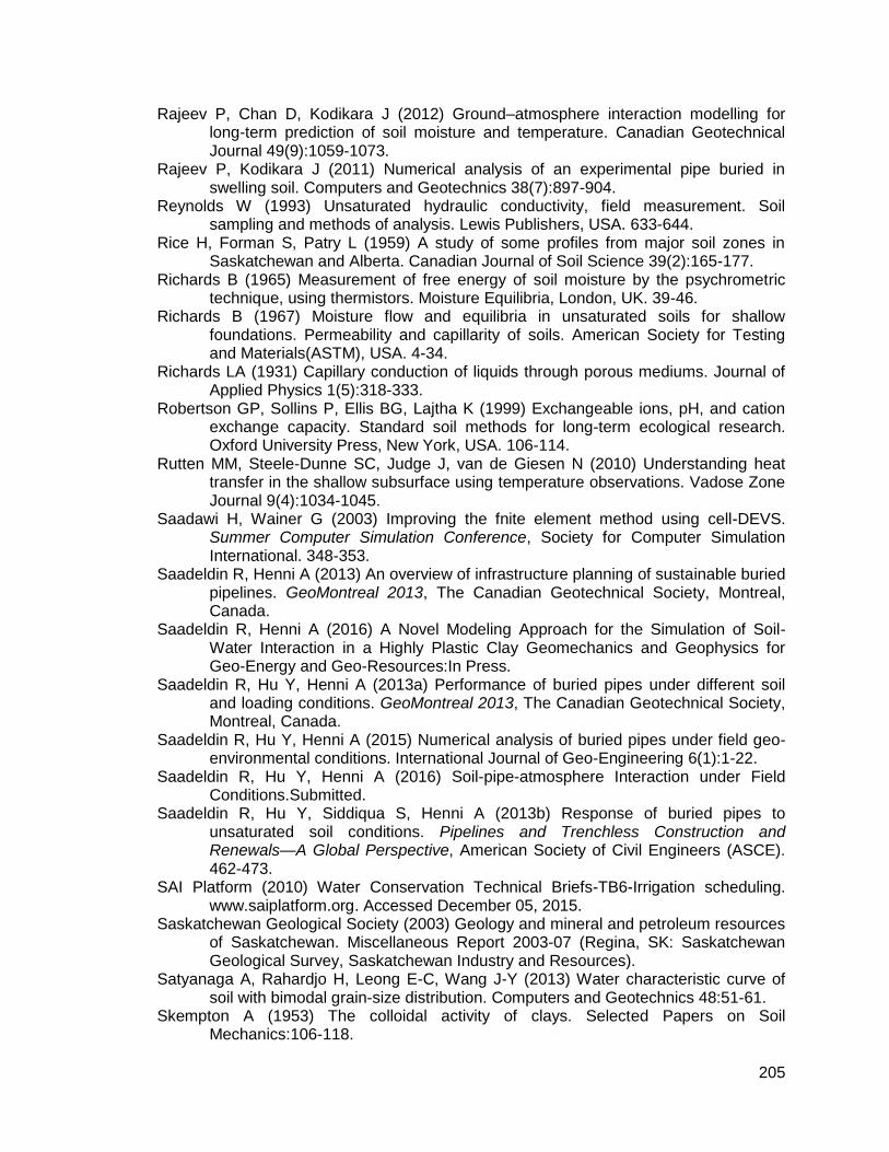
205
Rajeev P, Chan D, Kodikara J (2012) Ground–atmosphere interaction modelling for long-term prediction of soil moisture and temperature. Canadian Geotechnical Journal 49(9):1059-1073.
Rajeev P, Kodikara J (2011) Numerical analysis of an experimental pipe buried in swelling soil. Computers and Geotechnics 38(7):897-904.
Reynolds W (1993) Unsaturated hydraulic conductivity, field measurement. Soil sampling and methods of analysis. Lewis Publishers, USA. 633-644.
Rice H, Forman S, Patry L (1959) A study of some profiles from major soil zones in Saskatchewan and Alberta. Canadian Journal of Soil Science 39(2):165-177.
Richards B (1965) Measurement of free energy of soil moisture by the psychrometric technique, using thermistors. Moisture Equilibria, London, UK. 39-46.
Richards B (1967) Moisture flow and equilibria in unsaturated soils for shallow foundations. Permeability and capillarity of soils. American Society for Testing and Materials(ASTM), USA. 4-34.
Richards LA (1931) Capillary conduction of liquids through porous mediums. Journal of Applied Physics 1(5):318-333.
Robertson GP, Sollins P, Ellis BG, Lajtha K (1999) Exchangeable ions, pH, and cation exchange capacity. Standard soil methods for long-term ecological research. Oxford University Press, New York, USA. 106-114.
Rutten MM, Steele-Dunne SC, Judge J, van de Giesen N (2010) Understanding heat transfer in the shallow subsurface using temperature observations. Vadose Zone Journal 9(4):1034-1045.
Saadawi H, Wainer G (2003) Improving the fnite element method using cell-DEVS. Summer Computer Simulation Conference, Society for Computer Simulation International. 348-353.
Saadeldin R, Henni A (2013) An overview of infrastructure planning of sustainable buried pipelines. GeoMontreal 2013, The Canadian Geotechnical Society, Montreal, Canada.
Saadeldin R, Henni A (2016) A Novel Modeling Approach for the Simulation of Soil-Water Interaction in a Highly Plastic Clay Geomechanics and Geophysics for Geo-Energy and Geo-Resources:In Press.
Saadeldin R, Hu Y, Henni A (2013a) Performance of buried pipes under different soil and loading conditions. GeoMontreal 2013, The Canadian Geotechnical Society, Montreal, Canada.
Saadeldin R, Hu Y, Henni A (2015) Numerical analysis of buried pipes under field geo-environmental conditions. International Journal of Geo-Engineering 6(1):1-22.
Saadeldin R, Hu Y, Henni A (2016) Soil-pipe-atmosphere Interaction under Field Conditions.Submitted.
Saadeldin R, Hu Y, Siddiqua S, Henni A (2013b) Response of buried pipes to unsaturated soil conditions. Pipelines and Trenchless Construction and Renewals—A Global Perspective, American Society of Civil Engineers (ASCE). 462-473.
SAI Platform (2010) Water Conservation Technical Briefs-TB6-Irrigation scheduling. www.saiplatform.org. Accessed December 05, 2015.
Saskatchewan Geological Society (2003) Geology and mineral and petroleum resources of Saskatchewan. Miscellaneous Report 2003-07 (Regina, SK: Saskatchewan Geological Survey, Saskatchewan Industry and Resources).
Satyanaga A, Rahardjo H, Leong E-C, Wang J-Y (2013) Water characteristic curve of soil with bimodal grain-size distribution. Computers and Geotechnics 48:51-61.
Skempton A (1953) The colloidal activity of clays. Selected Papers on Soil Mechanics:106-118.

206
Skempton A (1961) Effective stress in soils, concrete and rocks. Pore pressure and suction in soils. Butterworths, London, UK. 4–16.
Soil Science Society of America (2008) Glossary of soil science terms. SSSA, Madison, WI, USA.
Stearn CW, Carroll RL, Clark TH (1979) Geological evolution of North America. John Wiley & Sons, Wiley, USA. 545.
Suleiman MT (2002) The structural performance of flexible pipes. Iowa State University. Ames, Iowa 160.
Terzaghi VK (1936) The shearing resistance of saturated soils and the angle between the planes of shear. Proceedings of the 1st international conference on soil mechanics and foundation engineering, Harvard University Press Cambridge, MA. 54-56.
Thomas PJ (1998) Quantifying properties and variability of expansive soils in selected map units. Virginia Polytechnic Institute and State University. Virginia, USA.
Trenhaile AS (2004) Geomorphology: a Canadian perspective. Don Mills, Ont.: Oxford University Press, New York, USA.
Trickey SA, Moore ID (2007) Three-dimensional response of buried pipes under circular surface loading. Journal of Geotechnical and Geoenvironmental Engineering 133(2):219-223.
Uni-Bell PVC Pipe Association (1991) Handbook of PVC pipe: design and construction. Uni-Bell PVC Pipe Association, Dallas, TX, USA. 474.
Van Der Merwe D (1964) The prediction of heave from the plasticity index and the percentage clay fraction of soils. 6(6):103-107.
Vanapalli S, Pufahl D, Fredlund D (1998) The effect of stress state on the soil-water characteristic behavior of a compacted sandy-clay till. Proceedings of the 51st Canadian Geotechnical Conference, Edmonton, Canada. 81-86.
Veihmeyer FJ (1964) Evapotranspiration. Hand Book of Applied Hydrology. McGraw-Hill, New York, USA. 11.11-11.38.
Vu HQ, Fredlund DG (2004) The prediction of one-, two-, and three-dimensional heave in expansive soils. Canadian Geotechnical Journal 41(4):713-737.
Wallace WS (1948) Geology of Canada vol 3. University Associates of Canada, Toronto, Canada. 23-26.
Walsh KD, Colby CA, Houston WN, Houston SL (2009) Method for evaluation of depth of wetting in residential areas. Journal of geotechnical and geoenvironmental engineering 135(2):169-176.
Wang J-J, Zhu J-G, Chiu C, Zhang H (2007) Experimental study on fracture toughness and tensile strength of a clay. Engineering Geology 94(1):65-75.
Watkins RK, Anderson LR (1999) Structural mechanics of buried pipes. CRC Press, Boca Raton, USA. 444.
Wheeler S, Karube D (1995) State of the art report: Constitutive modelling. The First International Conference on Unsaturated Soils, Paris, France. 1323-1356.
White NF, Duke HR, Sunada DK, Corey AT (1970) Physics of desaturation in porous materials. Journal of the Irrigation and Drainage Division 96(2):165-191.
White WA (1949) Atterberg plastic limits of clay minerals. American Mineralogist 34:508-512.
Wijewickreme D (2012) Role of geotechnical engineering in assuring the integrity of buried pipeline systems. International Conference on Sustainable Built Environment (ICSBE), Kandy, Sri Lanka.
Wijewickreme D, Weerasekara L (2010) Pipeline geotechnical engineering. Encyclopedia of Life Support Systems (EOLSS). www.eolss.net/sample-chapters. Accessed July 01, 2015.

207
Wilson G, Fredlund D, Barbour S (1997) The effect of soil suction on evaporative fluxes from soil surfaces. Canadian Geotechnical Journal 34(1):145-155.
Wilson G, Fredlund M (2000) The application of knowledgebased surface flux boundary modeling. Unsaturated soils for Asia. Toll&Leong (Eds), Proceedings of the Asian Conference on Unsaturated Soils, UNSAT-Asia 2000, Singapore.
Wilson GW (1990) Soil evaporative fluxes for geotechnical engineering problems. PhD. Dissertation, University of Saskatchewan. Saskatoon, Canada.
Wilson GW, Fredlund D, Barbour S (1994) Coupled soil-atmosphere modelling for soil evaporation. Canadian Geotechnical Journal 31(2):151-161.
Winkler E (1867) Theory of elasticity and strength. Dominicus Prague (in German). Czechoslovakia.
Wulfsohn D, Adams B, Fredlund D (1996) Application of unsaturated soil mechanics for agricultural conditions. Canadian Agricultural Engineering 38(3):173-181.
Yesiller N, Miller C, Inci G, Yaldo K (2000) Desiccation and cracking behavior of three compacted landfill liner soils. Engineering Geology 57(1):105-121.
Yong RN, Warkentin BP (1966) Introduction to soil behavior. Series in Civil Engineering. Macmillan, New York, USA. 451.
Young MH, Sisson JB (2002) Tensiometry. Methods of Soil Analysis: Part 4 Physical Methods. Soil Science Society of America, USA. 575-678.
Young W, Budynas R, Sadegh A (2011) Roark's formulas for stress and strain. McGraw Hill Professional, New York, USA.
Zarghamee MS (1986) Buried flexible pipe with nonuniform soil support. Journal of transportation engineering 112(4):400-415.
Zhan C, Rajani B (1997) Load transfer analyses of buried pipe in different backfills. Journal of transportation engineering 123(6):447-453.
Zhang L, Chen Q (2005) Predicting bimodal soil–water characteristic curves. Journal of Geotechnical and Geoenvironmental Engineering 131(5):666-670.
Zhang X (2004) Consolidation theories for saturated-unsaturated soils and numerical simulations of residential buildings on shrink-swell soils. Department of Civil Engineering, Texas A&M University. College Station, TX, USA.
Zhao JQ, Kuraoka S, Baker T, Gu P, Masson J, Boudreau S, Brousseau R (1998) Durability and Performance of Gravity Pipes: A State-of-the-Art Literature Review. Institute for Research in Construction , National Research Council of Canada, Ottawa, Canada. 60.
Zotarelli L, Dukes MD, Romero CC, Migliaccio KW, Morgan KT (2014) Step by step calculation of the Penman-Monteith Evapotranspiration (FAO-56 Method). Agricultural and Biological Engineering Department, Florida Cooperative Extension Service, Institute of Food and Agricultural Sciences, University of Florida, Florida, USA.

208
APPENDIX
A.1: Modeling Load-deformation Analysis (Selected Samples)
Figure A.1.1: Vertical displacement distribution due to surface loading of 50 kPa (Case Description: Pipe diameter = 300mm, E = Es)
Figure A.1.2: Vertical displacement distribution due to surface loading of 50 kPa (Case Description: Pipe diameter = 300mm, no trench configuration, E = 5Es)

209
Figure A.1.3: Vertical displacement distribution due to surface loading of 50 kPa (Case Description: Pipe diameter = 300 mm, with trench configuration, E = 5Es)

210
A.2: Modeling Partial Saturation Analysis (Selected Results)
A.2.1: Vertical heave distribution due to change of soil suction of around 2000 kPa (Fixed-fixed end restrains)
Figure A.2.2: Vertical heave distribution due to change of soil suction of 1000 kPa (Fixed-fixed end restrains)

211
Figure A.2.3: Vertical heave distribution due to a change in soil suction of 1000 kPa (Hinged-hinged end restrains)
Figure A.2.4: Vertical heave distribution due to a change of soil suction of 2000 kPa (Hinged-hinged end restrains)

212
A.3: Soil Column Modeling (Selected Results)
Figure A.3.1: VWC mapping at elapsed time of 30 days (I=0.01 and fmax = 50)
Figure A.3.2: VWC mapping at elapsed time of 90 days (I=0.01 and fmax = 50)

213
Figure A.3.3: VWC mapping at elapsed time of 120 days
Figure A.3.4: VWC mapping at elapsed time of 240 days

214
Figure A.3.5: Suction mapping at elapsed time of 30 days
Figure A.3.6: Suction mapping at elapsed time of 90 days

215
Figure A.3.7: Suction mapping at elapsed time of 120 days
Figure A.3.8: Suction mapping at elapsed time of 240 days

216
A.4: Field Site Modeling (Selected Results)
Figure A.4.1: VWC mapping at elapsed time of 5 days
Figure A.4.2: VWC mapping at elapsed time of 30 days

217
Figure A.4.3: VWC mapping at elapsed time of 140 days
Figure A.4.4: VWC mapping at elapsed time of 210 days

218
A.5: Field Site Location Map, Stratigraphic Cross Sections and Selected Photographs
Figure A.5.1: Site location Map
Emerald Park Road, Regina, Saskatchewan.
Project: Field Installation of an Instrumented Section of Water Main Pipe on Emerald
Park Road, October 24 to 31, 2005.
Center for Sustainable Infrastructure Research (CSIR). National Research Council
Canada.
Site Location

219
Fig
ure
A.5
.2: S
tratig
raph
ic c
ross s
ectio
n a
long
or n
ea
r 4th A
ve. (E
ast to
West) R
egin
a, S
askatc
hew
an
afte
r
(Fre
dlu
nd
, 1975)

220
Fig
ure
A.5
.3: S
tratig
raph
ic c
ross s
ectio
n a
long
or n
ea
r Alb
ert S
t. (No
rth to
So
uth
), Re
gin
a, S
askatc
hew
an a
fter
(Fre
dlu
nd
, 197
5)

221
Fig
ure
A.5
.4: S
tratig
raph
ic c
ross s
ectio
n a
long
or n
ea
r Vic
toria
Ave
. (Ea
st to
We
st), R
egin
a, S
askatc
hew
an
(Interpreted fro
m W
ater S
ecurity
Agency’s w
ate
r we
ll drille
r's re
ports
)
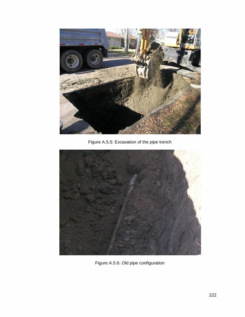
222
Figure A.5.5: Excavation of the pipe trench
Figure A.5.6: Old pipe configuration

223
Figure A.5.7: Placement of side support system
Figure A.5.8: Placement of the instrumented pipe

224
Figure A.5.9: Placement of soil pressure cells
Figure A.5.10: Placement of soil moisture sensors

225
Figure A.5.11: View of the site after the placement of the instrumented pipe
Figure A.5.12: View of the site showing the pavement cracks


