A note on wave equation in Einstein and de Sitter space-time · The metric of the Einstein and de...

A note on wave equation in Einstein and deSitter space-time

著者 Galstian Anahit, Kinoshita Tamotu, YagdjianKaren

journal orpublication title

Journal of mathematical physics

volume 51number 5page range 052501year 2010-05権利 (C) 2010 American Institute of PhysicsURL http://hdl.handle.net/2241/105409

doi: 10.1063/1.3387249

A note on wave equation in Einstein and de Sitterspace-time

Anahit Galstian,1,a� Tamotu Kinoshita,2,b� and Karen Yagdjian1,c�

1Department of Mathematics, University of Texas-Pan American, 1201 W. UniversityDrive, Edinburg, Texas 78541-2999, USA2Institute of Mathematics, University of Tsukuba, Tsukuba, Ibaraki 305-8571, Japan

�Received 17 August 2009; accepted 22 March 2010; published online 13 May 2010�

We consider the wave propagating in the Einstein and de Sitter space-time. Thecovariant d’Alembert’s operator in the Einstein and de Sitter space-time belongs tothe family of the non-Fuchsian partial differential operators. We introduce the ini-tial value problem for this equation and give the explicit representation formulas forthe solutions. We also show the Lp−Lq estimates for solutions. © 2010 AmericanInstitute of Physics. �doi:10.1063/1.3387249�

I. INTRODUCTION

The current note is concerned with the wave propagating in the universe modeled by thecosmological models with expansion. We are motivated by the significant importance of thesolutions of the partial differential equations arising in the cosmological problems for our under-standing of the universe. While there exists extensive literature on the hyperbolic equations, thequestion of initial value problems for the wave equation in the curved spaces with singularities,and, in particular, in the Einstein and de Sitter space-time, which are well posed and preservemany features of the classical waves, remains unresolved.

The homogeneous and isotropic cosmological models possess highest symmetry, which makesthem more amenable to rigorous study. Among them, Friedmann–Lemaître–Robertson–Walkermodels are mentioned. The simplest class of cosmological models can be obtained if we assumethat the metric of the slices of constant time is flat and that the space-time metric can be writtenin the form

ds2 = − dt2 + a2�t��dx2 + dy2 + dz2� ,

with an appropriate scale factor a�t�. �See, e.g. Ref. 22.� The assumption that the universe isexpanding leads to the positivity of the time derivative �d /dt�a�t�. The time dependence of thefunction a�t� is determined by the Einstein field equations for gravity,

R�� − 12g��R = − 8�GT��.

The metric of the Einstein and de Sitter universe �EdeS universe� is a particular member of theFriedmann–Robertson–Walker metrics,

ds2 = − dt2 + a2�t�� dr2

1 − Kr2 + r2d�2� ,

where K=−1, 0, or +1, for a hyperbolic, flat, or spherical spatial geometry, respectively. TheEinstein equations are simply

a�Electronic mail: [email protected]�Electronic mail: [email protected]�Electronic mail: [email protected].

JOURNAL OF MATHEMATICAL PHYSICS 51, 052501 �2010�

51, 052501-10022-2488/2010/51�5�/052501/18/$30.00 © 2010 American Institute of Physics

Downloaded 21 Jun 2010 to 130.158.56.101. Redistribution subject to AIP license or copyright; see http://jmp.aip.org/jmp/copyright.jsp

http://dx.doi.org/10.1063/1.3387249

http://dx.doi.org/10.1063/1.3387249

http://dx.doi.org/10.1063/1.3387249

� = − 3�� + p�a

a,

a

a= −

4�

3�� + 3p�, � a

a�2

=8�

3� −

K

a2 , �1.1�

where � is the proper energy density and p is pressure. For pressureless matter distributions �p=0� and vanishing spatial curvature �K=0� in the EdeS universe the solution to the Eqs. �1.1� is

a�t� = a0t2/3,

where a0 is an integration constant.19 This model describes an open geometry �the K=0 and spatialsections are diffeomorphic to R3� in the presence of a constant nonzero energy density distribution.Even though the EdeS space-time is conformally flat, its causal structure is quite different fromasymptotically flat geometries. In particular, and unlike Minkowski or Schwarzschild, the pastparticle horizons exist. The EdeS space-time is a good approximation to the large scale structureof the universe during a matter dominated phase, when the averaged �over space and time� energydensity evolves adiabatically and pressures are vanishingly small, as, e.g., immediately afterinflation.35 This justifies why such a metric is adopted to model the collapse of overdensityperturbations in the early matter dominated phase that followed inflation.

The Einstein and de Sitter model of the universe is the simplest nonempty expanding modelwith the line element,

ds2 = − dt2 + a02t4/3�dx2 + dy2 + dz2� ,

in comoving coordinates.11 It was first proposed jointly by Einstein and de Sitter �the EdeSmodel�.10 The observations of the microwave radiation fit in with this model.9 The result of thiscase also correctly describes the early epoch, even in a universe with curvature different from zero�Ref. 5, Sec. 8.2�. Recently it was used in Ref. 29 to study cosmological black holes. The keyobservation for that approach is that the line element can also be written in the conformally flatform,

ds2 = �4�− d�2 + dr2 + r2�d�2 + sin2 �d�2�� ,

where the timelike coordinates are related by d� /dt= �3t�−2/3. The last form is an asymptotic forthe Schwarzschild metric whose line element may be written in the form

ds2 = �4�− �1 −2m

r�dt2 +

4m

rdtdr + �1 +

2m

r�dr2 + r2�d�2 + sin2 �d�2�� ,

where t and r are timelike and spacelike coordinates related to the standard Schwarzschild coor-dinates t and r by

t = t + 2m ln r

2m− 1, r = r .

The fact that the resulting metric is asymptotically Einstein and de Sitter with the source reducingto a comoving pure dust at null infinity is used in Ref. 29. In this sense the solution could beinterpreted as a black hole in the asymptotic background of the Einstein and de Sitter universe.

The covariant d’Alambert’s operator in the Einstein and de Sitter space-time is

�g = − � �

�t�2

+ t−4/3 i=1,2,3

� �

�xi�2

−2

t

�

�t .

Consequently, the covariant wave equation with the source term f written in the coordinates is

052501-2 Galstian, Kinoshita, and Yagdjian J. Math. Phys. 51, 052501 �2010�


� �

�t�2

− t−4/3 i=1,2,3

� �

�xi�2

+2

t

�

�t = f . �1.2�

The last equation belongs to the family of the non-Fuchsian partial differential equations. There isvery advanced theory of such equations �see, e.g., Ref. 18 and references therein�. In this note weinvestigate the initial value problem for this equation and give the representation formulas for thesolutions with any dimension n�N of the spatial variable x�Rn.

Equation �1.2� is strictly hyperbolic in the domain with t0. On the hypersurface t=0 itscoefficients have singularities that make the study of the initial value problem difficult. Then, thespeed of propagation is equal to t−2/3 for every t�R \ �0�. Equation �1.2� is not Lorentz invariant,which brings additional difficulties.

The classical works on the Tricomi and Gellerstedt equations �see, e.g., Refs. 4, 6, 8, and 31�appeal to the singular Cauchy problem for the Euler–Poisson–Darboux equation,

�u = utt +c

tut, c � C , �1.3�

and to the Asgeirsson mean value theorem when handling a high-dimensional case. Here � is theLaplace operator on the flat metric, �ªi=1

n ��2 /�xi2�.

We use the approach suggested in Ref. 32 and reduce the problem for Eq. �1.2� to the Cauchyproblem for the free wave equation in Minkowski space-time: vtt−�v=0. To us, this approachseems to be more immediate than the one that uses the Euler–Poisson–Darboux equation. Moreprecisely, in the present note we utilize the solution v=v�x , t ;b� to the Cauchy problem,

vtt − �v = 0, t 0, x � Rn

v�x,0� = ��x,b� , vt�x,0� = 0, x � Rn,� �1.4�

with the parameter b�B�R. We denote that solution by v�=v��x , t ;b�. In the case of function �independent of parameter, we skip b and simply write v�=v��x , t�. There are well-known explicitrepresentation formulas for the solution of the last problem. We write those formulas to make thepresent note self-contained. If n=1, and ��x , t�= f�x , t��C �R�R�, B=R, then

v f�x,t;b� = 12 �f�x + t,b� + f�x − t,b��, t � R, x � R . �1.5�

For f �C �Rn�R� and for odd n=2m+1, m�N,

v f�x,t;b� =�

�t�1

t

�

�t��n−3�/2 tn−2

�n−1c0�n��

Sn−1f�x + ty,b�dSy, t � R, x � Rn, �1.6�

where, c0�n�=1·3 ·5 · . . . · �n−2�, while for x�Rn with even n=2m, m�N,

v f�x,t;b� =�

�t�1

t

�

�t��n−2�/2 2tn−1

�n−1c0�n��

B1n�0�

1�1 − �y�2

f�x + ty,b�dVy, t � R, x � Rn, �1.7�

where c0�n�=1·3 ·5 · . . . · �n−1�. �See, e.g., Theorems 4.1,4.2.24� In particular, if f is independent of

t, then v f�x , t ;b� does not depend on b and we briefly write v f�x , t�.The straightforward application of the formulas obtained in Ref. 32 to the Cauchy problem for

Eq. �1.2� decidedly does not work, but it reveals a surprising link to the Einstein and de Sitterspace-time. To demonstrate that link we note that the “principal part” of Eq. �1.2� belongs to thefamily of the Tricomi-type equations �in the case of odd l it is Gellerstedt equation�,

utt − tl�u = 0,

where l�N. According to Ref. 32 the solution to the Cauchy problem,

052501-3 Wave equation in Einstein and de Sitter space-time J. Math. Phys. 51, 052501 �2010�


utt − tl�u = f�x,t�, u�x,0� = �0�x�, ut�x,0� = �1�x� ,

with the smooth functions f , �0, and �1 can be represented as follows:

u�x,t� = 22−2��2��2�� 0

1

�1 − s2��−1v�0�x,��t�s�ds

+ t22��2 − 2��2�1 − �� 0

1

�1 − s2�−�v�1�x,��t�s�ds

+ 2ck�0

t

db�0

��t�−��b�

drE�r,t;0,b�v f�x,r;b�, x � Rn, t 0, �1.8�

with the kernel

E�r,t;0,b� ª ��b� + ��t��2 − r2�−�F��,�;1;��t� − ��b��2 − r2

��t� + ��b��2 − r2� . �1.9�

Here F�� ,� ;1 ;�� is the hypergeometric function �see, e.g., Ref. 1�, while kª l /2, ��t�ª t�k+1� / �k+1�, �ªk / �2k+2�, and ck= �k+1�−k/�k+1�2−1/�k+1�. The equation with l�N, x�R, andf =0 is studied in Ref. 30 by means of the partial Fourier transform and the confluent hypergeo-metric function. That approach gives parametrix of the Cauchy problem, and as a consequence, acomplete description of the propagation of the C -singularities.

Suppose now that we are looking for the simplest possible kernel E�r , t ;0 ,b� �1.9� of the lastintegral transform. In the hierarchy of the hypergeometric functions the simplest one, that isdifferent from the constant, is a linear function. That simplest function F�a ,b ;1 ;�� has the pa-rameters a=b=−1 and coincides with 1+�. The parameter l leading to such function F�−1,−1;1 ;��=1+� is exactly the exponent l=−4 /3 of the wave equation �and of the metric tensor� inthe Einstein and de Sitter space-time.

It is evident that the first term of the representation �1.8�, as it is written, is meaningless if�=−1. This indicates the fact that the Cauchy problem is not well posed anymore for the equationwith l=−4 /3. The next theorem also shows how the “lower order term” of Eq. �1.2� affects theCauchy problem. The main result of this paper is the following theorem.

Theorem 1.1: Assume that �i�C�n/2�+3−i�Rn�, i=0,1, f�x , t��C�n/2�+2�Rn� �0, ��, and thatwith some �0 one has

��x�f�x,t�� + �t�t�x

�f�x,t�� C�t�−2 for all x � Rn, and for all small t 0,

and for every �, �, �� n /2�+2 , �� n /2�+1. Then the solution =�x , t� to the problem,

tt − t−4/3� + 2t−1t = f�x,t�, t 0, x � Rn

limt→0

t�x,t� = �0�x�, limt→0

�tt�x,t� + �x,t� + 3t−1/3��0�x�� = �1�x�, x � Rn,��1.10�

is given by

�x,t� =3

2t2�

0

1

db�0

1−b1/3

dsbv f�x,3t1/3s;tb��1 + b2/3 − s2�

+ t−1v�0�x,3t1/3� − 3t−2/3��tv�0

��x,3t1/3� +3

2�

0

1

v�1�x,3t1/3s��1 − s2�ds . �1.11�

The theorem shows that one cannot anticipate the well posedness in the Cauchy problem for thewave equation in the Einstein and de Sitter space-time. In fact, it gives a structure of singularity ofthe solution at the point t=0, which hints at the proper initial conditions which have to be



prescribed for the solution. The initial conditions prescribed in the previous theorem are theCauchy conditions modified to the so-called weighted initial conditions in order to adjust them tothe equation. For the Euler–Poisson–Darboux equation �1.3� one can find such weighted initialconditions, for instance, in Refs. 4 and 25 as well as in the references therein. The existence anduniqueness of the solutions for the initial value problem with the weighted initial conditions forthe Euler–Poisson–Darboux equation and for Eq. �1.3� with the time-dependent c are proven inRef. 7 by application of the Fourier transform in x-variable, as well as some transformations whichreduce the equation to the confluent hypergeometric equation.

Theorem 1.1 can be used to obtain some important properties for the solutions of the waveequation in Einstein and de Sitter space-time, which are inherited from the solutions of the waveequation in Minkowski space-time. In particular, as a consequence of the previous theorem, inSec. III, for the initial value problem �1.10� with n�2, f =0, and �0=0, we obtain the followingLp−Lq estimate:

��− ��−s�· ,t��Lq�Rn� � Ct�1/3��2s−n�1/p−1/q��1�Lp�Rn�, t 0,

provided that s�0, 1� p�2, 1 / p+1 /q=1, �1 /2��n+1��1 / p−1 /q��2s�n�1 / p−1 /q�, andn�1 / p−1 /q�−1�2s. Similar estimates hold for the problem with general �0 and f . Thus, in thepresent paper we prepare all necessary tools that will allow us to study in the forthcoming paperthe solvability of semilinear wave equation in the Einstein and de Sitter space-time. Having inmind the scale invariance of the equation and also the applications �see, e.g., Refs. 16 and 28�,special attention will be given to the self-similar solutions. Results analogous to those presented inthis note have already proven to be a good tool in the study of self-similar solutions.35

This note is organized as follows. In Sec. II we prove the main theorem and give some of itsextensions �Theorems 2.1 and 2.2� that allow stronger singularity in the source term. Section III isdevoted to the application of the main theorem, namely, to the derivation of the Lp−Lq estimates.

The EdeS model recently became a focus of interest for an increasing number of authors. �See,e.g., Refs. 2, 11–15, 22, 23, and 29 and references therein.� We believe that the initial valueproblem and the explicit representation formulas obtained in the present paper fill the gap in theexisting literature on the wave equation in the EdeS space-time.

II. PROOF OF THE MAIN THEOREM

If we denote

L ª �t2 − t−4/3� + 2t−1�t, S ª �t

2 − t−4/3� ,

then we can easily check for t�0 the following operator identity:

t−1 � S � t = L . �2.1�

The last equation suggests a change of the unknown function with u such that = t−1u. Then theproblem for u is as follows:

�utt − t−4/3�u = g�x,t�, t 0, x � Rn

limt→0

u�x,t� = �0�x�, x � Rn

limt→0

�ut�x,t� + 3t−1/3��0�x�� = �1�x�, x � Rn,� �2.2�

where g�x , t�= tf�x , t�. Therefore it is enough to find a representation of the solution of the lastproblem. We discuss it in three separate cases of: �f� with �0=�1=0; ��0� with f =0 and �1=0;��1� with f =0 and �0=0.



We will use the following property of the resolving operator of the problem �1.4�: if P= P�Dx� is a pseudodifferential operator and �=��t� is a smooth function of time, then the operator��t�P�Dx� “commutes” with the resolving operator of the problem �1.4�. More precisely, thefollowing identity can easily be verified:

v�P�Dx�f�x,t;b� = ��b�P�Dx�v f�x,t;b� for all f � C �Rn � �0, �� . �2.3�

The operator S belongs to the family of the Tricomi-type operators,

T ª �t2 − tl� ,

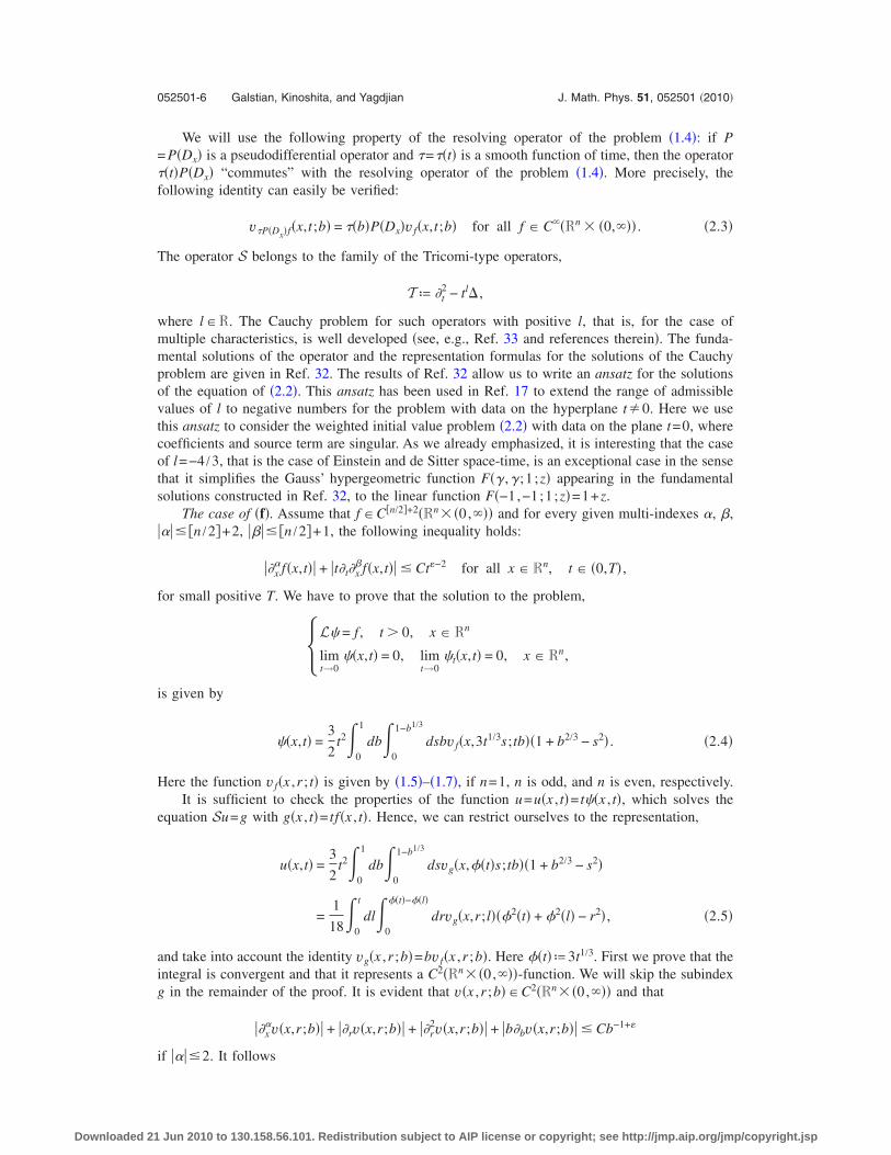
where l�R. The Cauchy problem for such operators with positive l, that is, for the case ofmultiple characteristics, is well developed �see, e.g., Ref. 33 and references therein�. The funda-mental solutions of the operator and the representation formulas for the solutions of the Cauchyproblem are given in Ref. 32. The results of Ref. 32 allow us to write an ansatz for the solutionsof the equation of �2.2�. This ansatz has been used in Ref. 17 to extend the range of admissiblevalues of l to negative numbers for the problem with data on the hyperplane t�0. Here we usethis ansatz to consider the weighted initial value problem �2.2� with data on the plane t=0, wherecoefficients and source term are singular. As we already emphasized, it is interesting that the caseof l=−4 /3, that is the case of Einstein and de Sitter space-time, is an exceptional case in the sensethat it simplifies the Gauss’ hypergeometric function F�� ,� ;1 ;z� appearing in the fundamentalsolutions constructed in Ref. 32, to the linear function F�−1,−1;1 ;z�=1+z.

The case of �f�. Assume that f �C�n/2�+2�Rn� �0, �� and for every given multi-indexes �, �,�� n /2�+2, �� n /2�+1, the following inequality holds:

��x�f�x,t�� + �t�t�x

�f�x,t�� Ct�−2 for all x � Rn, t � �0,T� ,

for small positive T. We have to prove that the solution to the problem,

L = f , t 0, x � Rn

limt→0

�x,t� = 0, limt→0

t�x,t� = 0, x � Rn,�is given by

�x,t� =3

2t2�

0

1

db�0

1−b1/3

dsbv f�x,3t1/3s;tb��1 + b2/3 − s2� . �2.4�

Here the function v f�x ,r ; t� is given by �1.5�–�1.7�, if n=1, n is odd, and n is even, respectively.It is sufficient to check the properties of the function u=u�x , t�= t�x , t�, which solves the

equation Su=g with g�x , t�= tf�x , t�. Hence, we can restrict ourselves to the representation,

u�x,t� =3

2t2�

0

1

db�0

1−b1/3

dsvg�x,��t�s;tb��1 + b2/3 − s2�

=1

18�

0

t

dl�0

��t�−��l�

drvg�x,r;l��2�t� + �2�l� − r2� , �2.5�

and take into account the identity vg�x ,r ;b�=bv f�x ,r ;b�. Here ��t�ª3t1/3. First we prove that theintegral is convergent and that it represents a C2�Rn� �0, ��-function. We will skip the subindexg in the remainder of the proof. It is evident that v�x ,r ;b��C2�Rn� �0, �� and that

��x�v�x,r;b�� + ��rv�x,r;b�� + ��r

2v�x,r;b�� + �b�bv�x,r;b�� Cb−1+�

if ��2. It follows



�v�x,��t�s;tb�� Ct−1+�b−1+�.

Then we use the last inequality and the first formula of �2.5� in the following inequalities:

�u�x,t�� Ct1+��0

1

b−1+�db�0

1−b1/3

ds�1 + b2/3 − s2� � C�t1+�. �2.6�

The first formula of �2.5� leads to the estimate for the derivative,

�

�tu�x,t� � 3t�

0

1

db�0

1−b1/3

dsv�x,��t�s;tb��1 + b2/3 − s2�+ 3

2t4/3�

0

1

db�0

1−b1/3

dss��rv��x,��t�s;tb��1 + b2/3 − s2�+ 3

2t2�

0

1

db�0

1−b1/3

dsb��bv��x,��t�s;tb��1 + b2/3 − s2� ,

that implies

�

�tu�x,t� � C�t��

0

1

b−1+�db�0

1−b1/3

ds�1 + b2/3 − s2�

+ C�t1/3+��0

1

b−1+�db�0

1−b1/3

dss�1 + b2/3 − s2�

+ C�t��0

1

b−1+�db�0

1−b1/3

ds�1 + b2/3 − s2� . �2.7�

Thus, the estimates �2.6� and �2.7� lead to the initial conditions

limt→0

u�x,t� = 0, limt→0

ut�x,t� = 0. �2.8�

It remains to verify the equation. For the derivative �� /�t�u�x , t� we use the second formula of�2.5� and obtain

�

�tu�x,t� = ��t�

1

18�

0

t

v�x,��t� − ��l�;l��2�t� + �2�l� − ��t� − ��l��2�dl

+ 2��t��t�1

18�

0

t

dl�0

��t�−��l�

drv�x,r;l�

=1

18��2�t��

0

t

v�x,��t� − ��l�;l��l�dl

+1

18��2�t��

0

t

dl�0

��t�−��l�

drv�x,r;l� .

For the second order derivative ��2 /�t2�u�x , t�, since 118��2�t��v�x ,0 ; t��t�=g�x , t� we derive

from the last equation



�2

�t2u�x,t� = g�x,t� +1

18��2�t��

0

t

v�x,��t� − ��l�;l��l�dl

+1

18��2�t��t��

0

t

vr�x,��t� − ��l�;l��l�dl +1

18��2�t��

0

t

dl�0

��t�−��l�

drv�x,r;l�

+1

18��2�t��t��

0

t

v�x,��t� − ��l�;l�dl . �2.9�

By means of the second formula of �2.5� and equation of �1.4� for the function �u we derive

�u�x,t� =1

18�

0

t

dl�0

��t�−��l�

dr�r2v�x,r;l��2�t� + �2�l� − r2� .

It follows

�u�x,t� =1

9��t��

0

t

�rv�x,��t� − ��l�;l��l�dl −1

18�

0

t

�rv�x,0;l��2�t� + �2�l��dl

+1

9�

0

t

dl�0

��t�−��l�

drr�rv�x,r;l� .

Since �rv�x ,0 ; l�=0, one more integration by parts yields

�u�x,t� =1

9��t��

0

t

�rv�x,��t� − ��l�;l��l�dl +1

9�

0

t

v�x,��t� − ��l�;l��t� − ��l��dl

−1

9�

0

t

dl�0

��t�−��l�

drv�x,r;l� . �2.10�

Hence according to �2.9� and �2.10� the application of the operator �t2− t−4/3� to the function u

=u�x , t� gives

utt�x,t� − t−4/3�u�x,t� = g�x,t� +1

18��2�t��

0

t

v�x,��t� − ��l�;l��l�dl

+1

18��2�t��t��

0

t

vr�x,��t� − ��l�;l��l�dl

+1

18��2�t��t��

0

t

v�x,��t� − ��l�;l�dl

− t−4/3 1

9��t��

0

t

vr�x,��t� − ��l�;l��l�dl

+1

9�

0

t

v�x,��t� − ��l�;l��t� − ��l��dl�= g�x,t� +

1

18��2�t��

0

t

v�x,��t� − ��l�;l��l�dl

+1

18��2�t��t��

0

t

v�x,��t� − ��l�;l�dl



− t−4/31

9�

0

t

v�x,��t� − ��l�;l��t� − ��l��dl

= g�x,t� +1

18��2�t��t��

0

t

v�x,��t� − ��l�;l�dl

− t−4/31

9��t��

0

t

v�x,��t� − ��l�;l�dl

= g�x,t� .

Thus, for this case the theorem is proven.One can allow more strong singularity of the source function f at t=0. More precisely, one can

reduce the case with such singularity to the one of Theorem 1.1 if the initial condition is modified.That is done in the next theorem.

Theorem 2.1: Assume that f�x , t��C�n/2�+4�Rn� �0, ��, t2f�x , t��C�Rn� �0, �� and that

��x�f�x,t�� + �t�t�x

�f�x,t�� C�t−2 for all t � �0,T�, x � Rn,

and for every �, �, �� n /2�+4, �� n /2�+3. Denote f0�x�ª limt→0 t2f�x , t� and suppose thatwith some �0 for the functions f�x , t� and f0�x��C�n/2�+4�Rn� the following inequality is ful-filled:

��x��tf�x,t� − t−1f0�x�� + �t�t�x

��tf�x,t� − t−1f0�x�� C�t�−1 for all t � �0,T�, x � Rn,

and for every �, �, �� n /2�+2, �� n /2�+1.Then the solution =�x , t� of the problem,

tt − t−4/3� + 2t−1t = f�x,t�, t 0, x � Rn

limt→0

�t�x,t�� = 0, limt→0

�tt�x,t� + �x,t� − f0�x�ln t� = 0, x � Rn,� �2.11�

is given by

�x,t� =1

tf0�x��t� +

1

18t�

0

t

dl�0

��t�−��l�

dr��2�t� + �2�l� − r2�

� �lv f�x,r;l� − l−1v f0�x,r� + l−4/3��l��v f0

�x,r�� , �2.12�

where ��t�ª�0t ln sds .

Proof: Consider the new unknown function w�x , t�ªu− f0�x��t�. Then

Sw�x,t� = tf�x,t� − S�f0�x��t�� = tf�x,t� − �t−1f0�x� − t−4/3��t��f0�x�� = h�x,t� ,

where we have denoted

h�x,t� ª t�f�x,t� − t−2f0�x�� + t−4/3��t��f0�x� .

According to the condition of the theorem with some �0 we have

��x�h�x,t�� + �t�t�x

�h�x,t�� C�t�−1 for all t � �0,T�, x � Rn,

�, �, �� n /2�+2, �� n /2�+1, that allows us to write representation �2.5� for the solutionw=w�x , t�,



w�x,t� =1

18�

0

t

dl�0

��t�−��l�

drvh�x,r;l��2�t� + �2�l� − r2� . �2.13�

On the other hand, according to Theorem 1.1, the function w=w�x , t� satisfies initial conditions

limt→0

w�x,t� = 0, limt→0

wt�x,t� = 0. �2.14�

Consequently,

limt→0

u�x,t� = limt→0

�w�x,t� + f0�x��t�� = 0,

limt→0

�ut�x,t� − f0�x�ln t� = limt→0

wt�x,t� = 0.

For the function =�x , t�= t−1u�x , t� this implies the initial conditions of �2.11�. To prove repre-sentation formula �2.12�, we note that

vh�x,r;b� = vt�f�x,t�−t−2f0�x��+t−4/3��t��f0�x��x,r;b�

= vtf�x,t��x,r;b� − vt−1f0�x��x,r;b� + vt−4/3��t��f0�x��x,r;b�

= bv f�x,r;b� − b−1v f0�x,r;b� + b−4/3��b��v f0

�x,r;b�

= bv f�x,r;b� − b−1v f0�x,r� + b−4/3��b��v f0

�x,r� .

Then we use �2.13� to write

w�x,t� =1

18�

0

t

dl�0

��t�−��l�

dr��2�t� + �2�l� − r2��lv f�x,r;l� − l−1v f0�x,r� + l−4/3��l��v f0

�x,r�� .

Thus, the representation

u�x,t� = f0�x��t� +1

18�

0

t

dl�0

��t�−��l�

dr��2�t� + �2�l� − r2�

� �lv f�x,r;l� − l−1v f0�x,r� + l−4/3��l��v f0

�x,r��

implies �2.12�. Theorem is proven. �

The last theorem does not exhaust the possible singularities of the source terms. The nexttheorem gives behavior of the solution as t→0 if the source term is more singular.

Theorem 2.2: Assume that f�x , t��C�n/2�+4�Rn� �0, �� and that with number a� �2,8 /3� onehas taf�x , t��C�Rn� �0, �� and

��x�f�x,t�� + �t�t�x

�f�x,t�� C�t−a for all t � �0,T�, x � Rn,

and for every �, �, �� n /2�+4, �� n /2�+1. Denote f0�x�ª limt→0 taf�x , t� and suppose thatwith some �0 for the functions f = f�x , t� and f0= f0�x��C�n/2�+4�Rn� the following inequality isfulfilled:

��x��tf�x,t� − t1−af0�x�� + �t�t�x

��tf�x,t� − t1−af0�x�� C�t�−1 for all t � �0,T�, x � Rn,

and for every �, �, �� n /2�+2, �� n /2�+1. Denote ��t�ª �3−a�−1�2−a�−1t3−a.Then the solution =�x , t� of the problem,



�tt − t−4/3� + 2t−1t = f�x,t�, t 0, x � Rn

limt→0

�t�x,t� −1

�3 − a��2 − a�t3−af0�x�� = 0, x � Rn

limt→0

�tt�x,t� + �x,t� −1

2 − at2−af0�x�� = 0, x � Rn,� �2.15�

is given by

�x,t� =1

tf0�x��t� +

1

18t�

0

t

dl�0

��t�−��l�

dr��2�t� + �2�l� − r2�

� �lv f�x,r;l� − l1−av f0�x,r� + l−4/3��l��v f0

�x,r�� . �2.16�

Proof: Consider the new unknown function w�x , t�ªu− f0�x��t�. Then

Sw�x,t� = tf�x,t� − S�f0�x��t�� = tf�x,t� − �t1−af0�x� − t−4/3��t��f0�x�� = h�x,t� ,

where we have denoted

h�x,t� ª t�f�x,t� − t−af0�x�� + t−4/3��t��f0�x� .

According to the condition of the theorem with some �0 we have

��x�h�x,t�� + �t�x

�ht�x,t�� C�t�−1 for all t � �0,T�, x � Rn,

�, �, �� n /2�+2, �� n /2�+1, that allows us to write representation �2.13�. On the otherhand, according to Theorem 1.1, the function w=w�x , t� satisfies initial conditions �2.14�. Conse-quently,

limt→0

�u�x,t� − f0�x��t�� = limt→0

w�x,t� = 0,

limt→0

�ut�x,t� − f0�x��t�� = limt→0

wt�x,t� = 0.

For the function =�x , t�= t−1u�x , t� this implies the initial conditions,

limt→0

�t�x,t� − f0�x��t�� = 0, limt→0

�tt�x,t� + �x,t� − f0�x��t�� = 0,

which coincide with ones of �2.15�. To prove representation formula �2.16�, we note that

vh�x,r;b� = vt�f�x,t�−t−af0�x��+t−4/3��t��f0�x��x,r;b�

= vtf�x,t��x,r;b� − vt1−af0�x��x,r;b� + vt−4/3��t��f0�x��x,r;b�

= bv f�x,r;b� − b1−av f0�x,r� + b−4/3��b��v f0

�x,r� .

Then

w�x,t� =1

18�

0

t

dl�0

��t�−��l�

drvh�x,r;l��2�t� + �2�l� − r2�

=1

18�

0

t

dl�0

��t�−��l�

dr��2�t� + �2�l� − r2�


�x,r�� .

Thus, the following representation



u�x,t� = f0�x��t� +1

18�

0

t

dl�0

��t�−��l�

dr��2�t� + �2�l� − r2�


�x,r��

for the function u=u�x , t� implies �2.16�. Theorem is proven. �

The case of ��0�. In this case f =0 and �1=0. One can find in the literature different ap-proaches for the construction of the solutions of the Fuchsian and non-Fuchsian partial differentialequations. �See, e.g., Refs. 18 and 20.� The next two lemmas give for f =0 behavior of thesolutions of the equation of �1.10� near the point of singularity t=0 of the coefficients.

Lemma 2.3: For �0�C0�n/2�+3�Rn� the function

u�x,t� = v�0�x,3t1/3� − 3t1/3��rv�0

��x,3t1/3� �2.17�

solves the problem

Su = 0, x � Rn, t 0

limt→0

u�x,t� = �0�x�, limt→0

�ut�x,t� + 3t−1/3��0�x�� = 0, x � Rn.�Here v��x ,3t1/3� is the value of the solution v�x ,r� to the Cauchy problem for the wave equation,vrr−�v=0, v�x ,0�=��x�, vt�x ,0�=0, taken at the point �x ,r�= �x ,3t1/3� .

Proof: We verify it by straightforward calculations. It is evident that

�u�x,t� = �v�0�x,3t1/3� − 3t1/3��r�v�0

�x,r��r=3t1/3. �2.18�

Denote

v0�x,t� = v�0�x,3t1/3�, v1�x,t� = − 3t1/3��rv�0

�x,r��r=3t1/3.

Then, for the derivatives �tv0�x , t� and �t2v0�x , t� we have

�tv0�x,t� = t−2/3��rv�0�x,r��r=3t1/3,

�t2v0�x,t� = −

2

3t−5/3��rv�0

�x,r��r=3t1/3 + t−4/3��r2v�0

�x,r��r=3t1/3.

At the mean time for the derivatives �tv1�x , t� and �t2v1�x , t� we have

�tv1�x,t� = − t−2/3��rv�0�x,r��r=3t1/3 − 3t−1/3��r

2v�0�x,r��r=3t1/3,

�t2v1�x,t� =

2

3t−5/3��rv�0

�x,r��r=3t1/3 − 3t−1��r3v�0

�x,r��r=3t1/3.

Hence, for the first order derivative �tu�x , t� and for the second order derivative �t2u�x , t� we have

�tu�x,t� = − 3t−1/3��r2v�0

�x,r��r=3t1/3,

�t2u�x,t� = t−4/3��r

2v�0�x,r��r=3t1/3 − 3t−1��r

3v�0�x,r��r=3t1/3, �2.19�

respectively. Consequently, using �2.18� and �2.19�, and the definition of v� we obtain



�t2u�x,t� − t−4/3�u�x,t� = t−4/3��r

2v�0�x,r��r=3t1/3 − 3t−1��r

3v�0�x,r��r=3t1/3 − t−4/3��v�0

�x,r��r=3t1/3

+ 3t−1��r�v�0�x,r��r=3t1/3

= t−4/3��r2v�0

�x,r� − �v�0�x,r��r=3t1/3 − 3t−1��r��r

2v�0�x,r� − �v�0

�x,r��r=3t1/3

= 0.

Thus, the function u=u�x , t� solves the equation utt�x , t�− t−4/3�u�x , t�=0. Lemma is proven. �

Corollary 2.4: The function = t−1u�x , t� solves the problem (1.10) with �1=0 and with f =0,that is,

tt�x,t� − t−4/3��x,t� + 2t−1t�x,t� = 0

limt→0

t�x,t� = �0, limt→0

�tt�x,t� + �x,t� + 3t−1/3��0�x�� = 0, x � Rn.�In particular, the corollary shows that for the given dimension n�N Huygens’ principle is validfor some particular waves propagating in the Einstein and de Sitter model of the universe if andonly if it is valid for the waves propagating in Minkowski space-time �cf. with Refs. 26, 32, and36�.

The case of ��1�. In this case f =0 and �0=0.Lemma 2.5: For �1�C0

�n/2�+2�Rn� the function

u�x,t� = t3

2�

0

1

v�1�x,��t�s��1 − s2�ds, x � Rn, t 0, �2.20�

solves the problem

Su = 0, x � Rn, t 0

limt→0

u�x,t� = 0, limt→0

ut�x,t� = �1�x�, x � Rn.�Here v��x ,��t�s� is the value of the solution v�x ,r� to the Cauchy problem for the wave equation,vrr−�v=0, v�x ,0�=��x�, vt�x ,0�=0, taken at the point �x ,r�= �x ,��t�s�, while ��t�=3t1/3.

Proof: We prove the lemma by straightforward calculations. We have

u�x,t� = t3

2�

0

1

v�1�x,��t�s��1 − s2�ds =

1

18�

0

��t�

v�1�x,r��2�t� − r2�dr .

For the first order derivative we derive

�tu�x,t� = �t1

18�

0

��t�

v�1�x,r��2�t� − r2�dr =

1

3t−1/3�

0

��t�

v�1�x,r�dr ,

while for the second order derivative using the last equation and integration by parts, we obtain

�t2u�x,t� = −

1

9t−4/3�

0

��t�

v�1�x,r�dr +

1

3t−1v�1

�x,��t��

= −1

9t−4/3�v�1

�x,r�r�0��t� − �

0

��t�

r��rv�1��x,r�dr� +

1

3t−1v�1

�x,��t��

= −1

9t−4/3�v�1

�x,��t��t� − �0

��t�

r��rv�1��x,r�dr� +

1

3t−1v�1

�x,��t�� .

Consequently,



�t2u�x,t� =

1

9t−4/3�

0

��t�

r��rv�1��x,r�dr . �2.21�

At the same time, we have

�u�x,t� =1

18�

0

��t�

�v�1�x,r��2�t� − r2�dr . �2.22�

Then Eqs. �2.21� and �2.22� imply

utt�x,t� − t−4/3�u�x,t� =1

9t−4/3� r2

2��rv�1

��x,r��0��t� − �

0

��t� r2

2��r

2v�1��x,r�dr�

− t−4/3 1

18�

0

��t�

�v�1�x,r��2�t� − r2�dr

=1

9t−4/3��2�t�

2��rv�1

��x,��t�� − �0

��t� r2

2��r

2v�1��x,r�dr�

− t−4/3 1

18�

0

��t�

�v�1�x,r��2�t� − r2�dr

=1

18t−4/3�2�t��rv�1

��x,��t�� −1

18t−4/3�

0

��t�

r2��r2v�1

��x,r�dr

− t−4/3 1

18�

0

��t�

�v�1�x,r��2�t� − r2�dr

=1

2t−2/3��rv�1

��x,��t�� −1

2t−2/3�

0

��t�

�v�1�x,r�dr .

The definition of the function v�1suggests that the function u=u�x , t� solves the equation

utt�x,t� − t−4/3�u�x,t� =1

2t−2/3 ��rv�1

��x,��t�� − �0

��t�

��r2v�1

��x,r�dr� = 0.

Finally, we verify the second initial condition by means of the l’Hospital’s rule,

limt→0

ut�x,t� = limt→0

1

3t−1/3�

0

��t�

v�1�x,r�dr = lim

t→0v�1

�x,��t�� = v�1�x,0� = �1�x� .

Lemma is proven. �

Corollary 2.6: The function = t−1u�x , t� solves the problem (1.10) with �0=0 and withoutsource term f, that is,

tt − t−4/3� + 2t−1t = 0, t 0, x � Rn

limt→0

t�x,t� = 0, limt→0

�tt�x,t� + �x,t�� = �1�x�, x � Rn.�The last corollary completes the proof of Theorem 1.1. �

In particular, Corollary 2.4 and Corollary 2.6 show that, because of the integration in theformula �2.20�, for all n�N Huygens’ principle is not valid for waves propagating in the Einsteinand de Sitter model of the universe, unless �1=0 and f =0.



III. Lp−Lq ESTIMATES

The representation formula �1.11� of Theorem 1.1 can be used to reproduce for the solutionsof the wave equation in Einstein and de Sitter space-time some important properties which possessthe solutions of the wave equation in Minkowski space-time. Among them there are estimates ofthe norm of solution in various functional spaces, such as Lp, Sobolev spaces, Besov spaces, andothers. These estimates provide a useful tool to prove local and global in time existencetheorems.24,27,34,35

In this short note we derive such estimates in the Lebesgue spaces only. First we remind theseestimates. If n�2, then for the solution v=v�x , t� of the Cauchy problem for the wave equation inMinkowski space-time

vtt − �v = 0, v�x,0� = ��x�, vt�x,0� = 0, �3.1�

with ��x��C0 �Rn� one has �see, e.g., Refs. 3 and 21� the following so-called Lp−Lq decay

estimate:

��− ��−sv�· ,t��Lq�Rn� � Ct2s−n�1/p−1/q��Lp�Rn� for all t 0, �3.2�

provided that s�0, 1� p�2, 1 / p+1 /q=1, and �1 /2��n+1��1 / p−1 /q��2s�n�1 / p−1 /q�.Then, for the solution v=v�x , t� of the Cauchy problem for the wave equation,

vtt − �v = 0, v�x,0� = 0, vt�x,0� = ��x� , �3.3�

there is the Lp−Lq estimate

��− ��−sv�· ,t��Lq�Rn� � Ct2s+1−n�1/p−1/q��Lp�Rn� for all t 0, �3.4�

under the conditions s�0, 1� p�2, 1 / p+1 /q=1, and �1 /2��n+1��1 / p−1 /q�−1�2s�n�1 / p−1 /q�.

The case of ��0�. According to Theorem 1.1, for the problem with �1=0 and f =0 the function=�x , t� can be represented as follows:

�x,t� = t−1v�0�x,3t1/3� − 3t−2/3��tv�0

��x,3t1/3� . �3.5�

Here for �0�C0 �Rn� the function v�0

�x ,3t1/3� coincides with the value v�x ,3t1/3� of the solutionv�x , t� of the Cauchy problem �3.1�. Hence for s�0 by means of application of �3.2� we obtain

��− ��−sv�0�· ,3t1/3��Lq�Rn� � Ct�1/3��2s−n�1/p−1/q��0�Lp�Rn�, t 0.

To estimate the second term of �3.5� we apply �3.4� with s�0,

��− ��−s��rv�0��· ,3t1/3��Lq�Rn� � Ct�1/3��2s+1−n�1/p−1/q��0�Lp�Rn�, t 0,

provided that �1 /2��n+1��1 / p−1 /q�−1�2s�n�1 / p−1 /q�. Consequently, if s�0, 1� p�2,1 / p+1 /q=1, and �1 /2��n+1��1 / p−1 /q��2s�n�1 / p−1 /q�, then for the problem with �1=0 andf =0 we obtain

��− ��−s�· ,t��Lq�Rn� � Ct−1+�1/3��2s−n�1/p−1/q��0�Lp�Rn� + Ct−2/3t�1/3��2s+1−n�1/p−1/q��0�Lp�Rn�

� Ct�1/3��2s−n�1/p−1/q��t−1��0�Lp�Rn� + t−1/3��0�Lp�Rn��, t 0.

Thus, we have proven the following proposition.Proposition 3.1: Suppose that s�0, 1� p�2, 1 / p+1 /q=1, and �1 /2��n+1��1 / p−1 /q�

�2s�n�1 / p−1 /q�. Then the solution =�x , t� to the problem

tt − t−4/3� + 2t−1t = 0, t 0, x � Rn

limt→0

t�x,t� = �0�x�, limt→0

�tt�x,t� + �x,t� + 3t−1/3��0�x�� = 0, x � Rn,�



with �0�C0 �Rn� satisfies the following estimate:

��− ��−s�· ,t��Lq�Rn� � Ct�1/3��2s−1−n�1/p−1/q��t−2/3��0�Lp�Rn� + ��0�Lp�Rn��, t 0, �3.6�

with the constant C independent of �0.The case of ��1�. For the problem with �0=0 and f =0 the function =�x , t� due to Theorem

1.1 can be represented as follows:

�x,t� =3

2�

0

1

v�1�x,��t�s��1 − s2�ds, x � Rn, t 0.

Then we obtain for s, n, p, and q such that 2s−n�1 / p−1 /q�−1, the following estimate:

��− ��−s�· ,t��Lq�Rn� �3

2�

0

1

��− ��−sv�1�· ,��t�s��Lq�Rn��1 − s2�ds

� C�0

1

t�1/3��2s−n�1/p−1/q��s�2s−n�1/p−1/q��1�Lp�Rn��1 − s2�ds

� Ct�1/3��2s−n�1/p−1/q��1�Lp�Rn��0

1

s2s−n�1/p−1/q��1 − s2�ds .

Thus, in this case we have proven the following proposition.Proposition 3.2: Suppose that s�0, 1� p�2, 1 / p+1 /q=1, 2s−n�1 / p−1 /q�−1, and

�1 /2��n+1��1 / p−1 /q��2s�n�1 / p−1 /q�. Then the solution =�x , t� to the problem

tt − t−4/3� + 2t−1t = 0, t 0, x � Rn

limt→0

t�x,t� = 0, limt→0

�tt�x,t� + �x,t�� = �1�x�, x � Rn,�with �1�C0

�Rn� satisfies the following estimate:

��− ��−s�· ,t��Lq�Rn� � Ct�1/3��2s−n�1/p−1/q��1�Lp�Rn�, t 0, �3.7�

with the constant C independent of �1.The case of �f�. According to Theorem 1.1, for the problem with �0=0 and �1=0 the function

=�x , t� can be represented as follows:

�x,t� =3

2t2�

0

1

db�0

1−b1/3

d�bv f�x,3t1/3�;tb��1 + b2/3 − �2� .

Consequently, for the problem with �0=0, �1=0, and the function f satisfying conditions of thetheorem, by application of �3.2� we obtain

��− ��−s�· ,t��Lq�Rn� �3

2t2�

0

1

db�0

1−b1/3

d�b��− ��−sv f�· ,3t1/3�;tb��Lq�Rn��1 + b2/3 − �2�

� Ct2�0

1

db�0

1−b1/3

d�bt�1/3��2s−n�1/p−1/q��2s−n�1/p−1/q��f�· ,tb��Lp�Rn��1 + b2/3 − �2� .

For a=2s−n�1 / p−1 /q�−1 one has

�0

1−b1/3

�a�1 + b2/3 − �2�d� =2

�a + 1��a + 3��1 − b1/3�a+1�1 + �a + 1�b1/3 + b2/3� .

Hence,



��− ��−s�· ,t��Lq�Rn�

� Ct2+�1/3��2s−n�1/p−1/q��0

1

b�f�· ,tb��Lp�Rn�db�0

1−b1/3

�2s−n�1/p−1/q��1 + b2/3 − �2�d�

� Cn,p,q,st2+�1/3��2s−n�1/p−1/q��

0

1

b�f�· ,tb��Lp�Rn��1 − b1/3�a+1�1 + �a + 1�b1/3 + b2/3�db

� Cn,p,q,st2+�1/3��2s−n�1/p−1/q��

0

1

b�f�· ,tb��Lp�Rn��1 − b1/3�2s−n�1/p−1/q�+1db .

Thus, in this case we have proven the following proposition.Proposition 3.3: Suppose that s�0, 1� p�2, 1 / p+1 /q=1, 2s−n�1 / p−1 /q�−1, and

�1 /2��n+1��1 / p−1 /q��2s�n�1 / p−1 /q�, and that the function f satisfies conditions of Theorem1.1. Then for the solution =�x , t� to the problem,

tt − t−4/3� + 2t−1t = f�x,t�, t 0, x � Rn

limt→0

t�x,t� = 0, limt→0

�tt�x,t� + �x,t�� = 0, x � Rn,�the following estimate:

��− ��−s�· ,t��Lq�Rn� � Cn,p,q,st�1/3��2s−n�1/p−1/q��

0

t

��f�· ,��Lp�Rn�d�

holds with the constant Cn,p,q,s independent of f.

ACKNOWLEDGMENTS

This work was initiated during the first and third authors visit Institute of Mathematics of theUniversity of Tsukuba in June 2008. The first and the third authors would like to express theirgratitude to the University of Tsukuba for the financial support. They are especially grateful toProfessor Kajitani, Professor Wakabayashi, and Professor Isozaki for their hospitality. Finally, theauthors thank the referee for useful comments.

1 Bateman, H. and Erdelyi, A., Higher Transcendental Functions �McGraw-Hill, New York, 1954�, Vols. 1 and 2.2 Blanchard, A., “Cosmological parameters: where are we?” Astrophys. Space Sci. 290, 135 �2004�.3 Brenner, P., “On Lp−Lq, estimates for the wave-equation,” Math. Z. 145, 251 �1975�.4 Carroll, R. W. and Showalter, R. E., Singular and Degenerate Cauchy Problems. Mathematics in Science and Engineer-ing �Academic, New York, 1976�, Vol. 127.

5 Cheng, T.-P., Relativity, Gravitation And Cosmology: A Basic Introduction �Oxford University Press, Oxford, NY, 2005�.6 Delache, S. and Leray, J., “Calcul de la solution élémentaire de l’opérateur d’Euler-Poisson-Darboux et de l’opérateur deTricomi-Clairaut, hyperbolique, d’ordre 2,” Bull. Soc. Math. France 99, 313 �1971�.

7 Del Santo, D., Kinoshita, T., and Reissig, M., “Klein-Gordon type equations with a singular time-dependent potential,”Rend. Istit. Mat. Univ. Trieste 39, 141 �2007�.

8 Diaz, J. B. and Weinberger, H. F., “A solution of the singular initial value problem for the Euler-Poisson-Darbouxequation,” Proc. Am. Math. Soc. 4, 703 �1953�.

9 Dirac, P. A. M., “The large numbers hypothesis and the Einstein theory of gravitation,” Proc. R. Soc. London, Ser. A 365,19 �1979�.

10 Einstein, A. and de Sitter, W., “On the relation between the expansion and the mean density of the universe,” Proc. Natl.Acad. Sci. U.S.A. 18, 213 �1932�.

11 Ellis, G. and van Elst, H., NATO Advanced Study Institute on Theoretical and Observational Cosmology, Cargèse,France, NATO Science Series, Series C, Mathematical and Physical Sciences, Vol. 541 �Kluwer Academic, Boston,1999�.

12 Goncalves, S. M. C. V., “Black hole formation from massive scalar field collapse in the Einstein-de Sitter universe,”Phys. Rev. D 62, 124006 �2000�.

13 Gron, O. and Hervik, S., Einstein’s General Theory of Relativity: With Modern Applications in Cosmology �Springer,New York, 2007�.

14 Hawking, S. W. and Ellis, G. F. R., The Large Scale Structure of Space-Time, Cambridge Monographs on MathematicalPhysics, No. 1 �Cambridge University Press, London, 1973�.



http://dx.doi.org/10.1023/B:ASTR.0000022169.31100.a4

http://dx.doi.org/10.1007/BF01215290

http://dx.doi.org/10.2307/2032401

http://dx.doi.org/10.1098/rspa.1979.0003

http://dx.doi.org/10.1073/pnas.18.3.213

http://dx.doi.org/10.1073/pnas.18.3.213

http://dx.doi.org/10.1103/PhysRevD.62.124006

15 Hawley, J. F. and Holcomb, K. A., Foundations of Modern Cosmology �Cambridge University Press, New York, 1997�.16 Henriksen, R. N. and Wesson, P. S., “Self-similar space-times,” Astrophys. Space Sci. 53, 429 �1978�.17 Kinoshita, T. and Yagdjian, K., “On the Cauchy problem for wave equations with time-dependent coefficients,” Int. J.

Appl. Math. Stat. 13, 1 �2008�.18 Mandai, T., “Characteristic Cauchy problems for some non-Fuchsian partial differential operators,” J. Math. Soc. Jpn. 45,

511 �1993�.19 Ohanian, H. and Ruffini, R., Gravitation and Spacetime �Norton, New York, 1994�.20 Parenti, C. and Tahara, H., “Asymptotic expansions of distribution solutions of some Fuchsian hyperbolic equations,”

Publ. Res. Inst. Math. Sci. 23, 909 �1987�.21 Pecher, H., “Lp-abschätzungen und klassische Lösungen für nichtlineare Wellengleichungen.I,” Math. Z. 150, 159

�1976�.22 Peebles, P. J. E., Principles of Physical Cosmology �Princeton University Press, Princeton, NJ, 1993�.23 Rendall, A. D., Partial Differential Equations in General Relativity, Oxford Graduate Texts in Mathematics No. 16

�Oxford University Press, Oxford, 2008�.24 Shatah, J. and Struwe, M., Geometric Wave Equations, Courant Lecture Notes in Mathematics No. 2 �American Math-

ematical Society, Providence, RI, 1998�.25 Smirnov, M. M., Equations of Mixed Type, Translations of Mathematical Monographs No. 51 �American Mathematical

Society, Providence, R.I., 1978� �Translated from the Russian�.26 Sonego, S. and Faraoni, V., “Huygens’ principle and characteristic propagation property for waves in curved space-

times,” J. Math. Phys. 33, 625 �1992�.27 Strauss, W., CBMS Regional Conference Series in Mathematics �American Mathematical Society, Providence, RI, 1989�,

Vol. 73.28 Suginohara, T., Taruya, A., and Suto, Y., “Quasi-self-similar evolution of the two-point correlation function: Strongly

nonlinear regime in �0�1 universes,” Astrophys. J. 566, 1 �2002�.29 Sultana, J. and Dyer, C. C., “Cosmological black holes: A black hole in the Einstein-de Sitter universe,” Gen. Relativ.

Gravit. 37, 1347 �2005�.30 Taniguchi, K. and Tozaki, Y., “A hyperbolic equation with double characteristics which has a solution with branching

singularities,” Math. Japonica 25, 279 �1980�.31 Weinstein, A., “The singular solutions and the Cauchy problem for generalized Tricomi equations,” Commun. Pure Appl.

Math. 7, 105 �1954�.32 Yagdjian, K., “A note on the fundamental solution for the Tricomi-type equation in the hyperbolic domain,” J. Differ.

Equations 206, 227 �2004�.33 Yagdjian, K., The Cauchy Problem for Hyperbolic Operators. Multiple Characteristics. Micro-Local Approach �Akad-

emie Verlag, Berlin, 1997�.34 Yagdjian, K., “Global existence for the n-dimensional semilinear Tricomi-type equations,” Commun. Partial Differ. Equ.

31, 907 �2006�.35 Yagdjian, K., “Self-similar solutions of semilinear wave equation with variable speed of propagation,” J. Math. Anal.

Appl. 336, 1259 �2007�.36 Yagdjian, K. and Galstian, A., “Fundamental solutions for the Klein-Gordon equation in de Sitter space-time,” Commun.

Math. Phys. 285, 293 �2009�.



http://dx.doi.org/10.1007/BF00645031

http://dx.doi.org/10.2969/jmsj/04530511

http://dx.doi.org/10.2977/prims/1195175863

http://dx.doi.org/10.1007/BF01215233

http://dx.doi.org/10.1063/1.529798

http://dx.doi.org/10.1086/337956

http://dx.doi.org/10.1007/s10714-005-0119-7

http://dx.doi.org/10.1007/s10714-005-0119-7

http://dx.doi.org/10.1002/cpa.3160070108

http://dx.doi.org/10.1002/cpa.3160070108

http://dx.doi.org/10.1016/j.jde.2004.07.028

http://dx.doi.org/10.1016/j.jde.2004.07.028

http://dx.doi.org/10.1080/03605300500361511

http://dx.doi.org/10.1016/j.jmaa.2007.03.061

http://dx.doi.org/10.1016/j.jmaa.2007.03.061

http://dx.doi.org/10.1007/s00220-008-0649-4

http://dx.doi.org/10.1007/s00220-008-0649-4

A note on wave equation in Einstein and de Sitter space-time · The metric of the Einstein and de...

Documents

Transcript of A note on wave equation in Einstein and de Sitter space-time · The metric of the Einstein and de...