Computational Statistics and Data Analysis 53 (2009) 3593–3600

Contents lists available at ScienceDirect

Computational Statistics and Data Analysis

journal homepage: www.elsevier.com/locate/csda

Short communication

A note on the properties of power-transformed returns in long-memorystochastic volatility models with leverage effectAna Pérez a, Esther Ruiz b,∗, Helena Veiga ba Dpto. Economía Aplicada (Estadística y Econometría), Universidad de Valladolid, Spainb Dpto. Estadística, Universidad Carlos III de Madrid, Spain

a r t i c l e i n f o

Article history:Received 9 October 2008Received in revised form 11 February 2009Accepted 22 February 2009Available online 9 March 2009

a b s t r a c t

The autocorrelation function (acf) of powered absolute returns and their cross-correlationswith original returns are derived, for any value of the power parameter, in the context oflong-memory stochastic volatility models with leverage effect and Gaussian noises. Theseautocorrelations and cross-correlations generalize and correct recent results on the acf ofsquared and absolute returns.

© 2009 Elsevier B.V. All rights reserved.

1. Introduction

An increasingly popularmodel to represent the dynamic evolution of the volatility of financial returns is the long-memorystochastic volatilitymodelwith leverage effect, denoted by A-LMSVmodel. Thismodel is able to explain the high persistenceoften observed empirically in the sample autocorrelation function (acf) of squared returns, and the asymmetric responseof volatility to positive and negative shocks; see Nakajima and Omori (2008) and Takahashi et al. (2008) for recent resultson the importance of asymmetry in stochastic volatility models. On the other hand, in order to characterize adequately thedynamics of conditionally heteroscedastic returns, it is important to know not only the acf of squared returns but also of anypower of absolute observations; see, for example, He et al. (2002), Karanasos and Kim (2003, 2006) and Franq and Zakoïan(2008) for references where the autocorrelations of powers of absolute returns are of interest. Furthermore, the presenceof an asymmetric response of volatility to positive and negative returns shows up in non-zero cross-correlations betweenoriginal returns and future powers of absolute returns. Recently, Ruiz and Veiga (2008) derive the properties of the A-LMSVmodel with Gaussian errors and compare them with those of the FIEGARCH model. In particular, they derive, among othermoments, the acf of powers of absolute observations, |yt |c , and the cross-correlations between yt and |yt+k|c , for c = 1 and2, where c is the power parameter. However, the acf in expression (5) of their paper is not valid when c = 1, i.e. for absoluteobservations, although it is still valid when c = 2, i.e. for squared observations. In this note, we derive the expressions ofthe acf of the power-transformed returns, |yt |c , and of the cross-correlations between yt and |yt+k|c for any positive powerc > 0. Therefore, we generalize the results in Ruiz and Veiga (2008) allowing a more precise description of the dynamics ofreturns generated by A-LMSV models. Furthermore, when c = 1, we obtain, as a particular case, the acf of absolute returnswhich corrects the wrong expression in Ruiz and Veiga (2008). Finally, when c = 2, the acf of squared returns comes up andcoincides with the expression given in Ruiz and Veiga (2008).The rest of the note is organized as follows. Section 2 derives the acf and cross-correlations of |yt |c . In Section 3, we obtain

the particular cases of the autocorrelations for c = 1 and 2. Section 4 concludes the note.

∗ Corresponding address: Department of Statistics, Universidad Carlos III de Madrid, C/ Madrid 126, 28903 Getafe, Spain. Tel.: +34 916249851; fax: +34916249849.E-mail address: ortega@est-econ.uc3m.es (E. Ruiz).

0167-9473/$ – see front matter© 2009 Elsevier B.V. All rights reserved.doi:10.1016/j.csda.2009.02.026

3594 A. Pérez et al. / Computational Statistics and Data Analysis 53 (2009) 3593–3600

2. The acf of power-transformed returns and their cross-correlation with returns

Consider the Asymmetric Long-Memory Stochastic Volatility, A-LMSV(1, d, 0), model proposed by Ruiz andVeiga (2008),given by

yt = σ∗σtεt , (1)

and

(1− φL)(1− L)d log σ 2t = ηt , (2)

where yt is the return at time t and σ∗σt is its volatility. The parameter σ∗ is a scale parameter that avoids the inclusionof a constant in the log-volatility equation, (2); see So et al. (1997) for an interpretation of this parameter as the volatilityobtained when conditioning upon an average level of information arrival to the market. L is the lag operator such thatLxt = xt−1. The disturbances (εt , ηt+1)′ are assumed to have the following bivariate normal distribution(

εtηt+1

)∼ NID

[(00

),

(1 δσηδση σ 2η

)],

where δ, the correlation between the noises, represents the leverage effect and induces correlation between returns andfuture volatilities; see Harvey and Shephard (1996). The parameters φ and d satisfy the stationarity conditions, i.e. |φ| < 1and |d| < 0.5.As wementioned above, the dynamic properties of conditionally heteroscedastic series with leverage effect are reflected

in the acf of |yt |c , and in the cross-correlation function between yt and |yt+k|c . Next, we derive both functions for theA-LMSV(1, d, 0)model in (1) and (2).

2.1. Autocorrelations

Consider first the autocorrelation of order k of |yt |c which is given by

ρc(k) =γc(k)γc(0)

,

where γc(k) = Cov(|yt |c , |yt+k|c) and γc(0) = Var(|yt |c). Denote by ht the log-volatility process, i.e. ht = log σ 2t . Then, thepower-transformed returns can be written as

|yt |c = σ c∗ exp(cht2

)|εt |

c .

Note that, by definition, ht and εt are contemporaneously independent. Therefore, using the properties of the log-normaldistribution, the variance of |yt |c can be derived as follows

γc(0) = E(|yt |2c)−[E(|yt |c)

]2= σ 2c

∗E[exp (cht)]E

(|εt |

2c)− σ 2c∗

[E(exp

(cht2

))]2[E(|εt |c)]2

= σ 2c∗[E(|εt |c)]2 exp

(c2σ 2h4

)[κc exp

(c2σ 2h4

)− 1

], (3)

where κc =E(|εt |2c )[E(|εt |c )]2

and E(|εt |c) = 2c/20

(c2+

12

)0

(12

) , where 0(·) is the Gamma function. The expression of σ 2h , the variance ofthe log-volatility process, which is an ARFIMA(1, d, 0) process, can be found in Hosking (1981). Note that the expression ofVar(|yt |c) given by Ghysels et al. (1996) and subsequently by Ruiz and Veiga (2008) is not correct.The autocovariance of order k of the power-transformed returns is given by

γc(k) = E(|yt |c |yt+k|c)− E(|yt |c)E(|yt+k|c)

= σ 2c∗E(|εt+k|

c) {E [exp( c(ht + ht+k)2

)|εt |

c]− exp

(c2σ 2h4

)E(|εt |c)

}. (4)

The first expectation within the squared brackets in (4) cannot be directly decomposed into the product of expectationsdue to the correlation between ηt+1 and εt . Consequently, in order to isolate the disturbance ηt+1 in ht + ht+k, we consider

the following AR(∞) representation of the log-volatility, ht =∑∞

i=1 λiηt+1−i, with λ1 = 1 and λk =k−1∑i=0

0(i+d)0(i+1)0(d)φ

k−1−i.

A. Pérez et al. / Computational Statistics and Data Analysis 53 (2009) 3593–3600 3595

Note that in the short-memory case, when d = 0, λk = φk−1. Then, it turns out that ht + ht+k−λkηt+1 can be written downas the following linear combination

ht + ht+k − λkηt+1 =k−1∑i=1

λiηt+1+k−i +

∞∑i=1

(λi + λk+i)ηt+1−i,

which is independent of ηt+1 and Gaussian. Therefore, adding and subtracting λkηt+1 in the corresponding expectation in(4), we obtain the following result

E[exp

(c(ht + ht+k)

2

)|εt |

c]= E

[exp

(c(ht + ht+k − λkηt+1)

2

)]E[|εt |

c exp(cλkηt+12

)]. (5)

The first expectation in (5) can be obtained by noting that ht + ht+k − λkηt+1 is normal with zero mean and variance

Var(ht + ht+k − λkηt+1) = 2σ 2h [1+ ρh(k)]− λ2kσ2η ,

where ρh(k) is the autocorrelation of order k of the log-squared volatility, ht ; see Hosking (1981) for the expression of thisautocorrelation. Then, using once more the properties of the log-normal distribution, it turns out that

E[exp

(c(ht + ht+k − λkηt+1)

2

)]= exp

(c2σ 2h [1+ ρh(k)]

4

)exp

(−c2λ2kσ

2η

8

). (6)

The second expectation on the right-hand side of (5) can be obtained from Proposition 1 in the Appendix, as follows

E[|εt |

c exp(cλkηt+12

)]= exp

(c2λ2kσ

2η (1− δ

2)

8

)0(c + 1)0( c2 + 1

)2−c/2Φ ( c + 12

,12;c2A2k2

), (7)

where Ak =λkδση2 and Φ(·, ·; ·) is the degenerate hypergeometric function; see Section 9.21 of Gradshteyn and Ryzhik

(1994).Now, replacing (6) and (7) into (5), putting (5) back into (4) and using formula 8.335.1 of Gradshteyn and Ryzhik (1994),

the following expression of the autocovariance of |yt |c is obtained after some straightforward algebra

γc(k) = σ 2c∗ exp(c2σ 2h4

)[E(|εt |c)]2

[exp

(c2σ 2h ρh(k)

4

)exp

(−c2A2k2

)Φ

(c + 12

,12;c2A2k2

)− 1

]. (8)

Finally, dividing the autocovariance in (8) by the variance in (3), the expression of the acf of |yt |c is obtained as follows

ρc(k) =exp

(c2σ 2h ρh(k)

4

)exp

(−c2A2k2

)Φ

(c+12 ,

12 ;c2A2k2

)− 1

κc exp(c2σ 2h4

)− 1

, k ≥ 1. (9)

Note that when d = 0, the acf of the short-memory A-ARSV (1) model is obtained. On the other hand, if there is noleverage effect, i.e. δ = 0, then Ak = 0 and Φ

( c+12 ,

12 ; 0

)= 1. In this case, the acf of the symmetric LMSV(1, d, 0) model,

derived by Harvey (1998), is obtained as a particular case of (9).

2.2. Cross-correlations

The cross-correlation of order k between returns and future power-transformed absolute returns is given by

Corr(yt , |yt+k|c) =Cov(yt , |yt+k|c)

√Var(yt)Var(|yt+k|c)

. (10)

The variance of |yt |c has been derived above and it is given by expression (3). On the other hand, the marginal variance ofreturns is given by

Var(yt) = σ 2∗ exp(σ 2h

2

). (11)

Finally, the cross-covariance between yt and |yt+k|c can be derived by taking into account that E(yt) = 0 and usingsimilar arguments to those used to derive the acf above, as follows

Cov(yt , |yt+k|c) = E(yt |yt+k|c) = σ c+1∗ E[exp

(ht + cht+k

2

)εt |εt+k|

c]

= σ c+1∗E(|εt+k|c)E

[exp

(ht + c(ht+k − λkηt+1)

2

)]E[εt exp

(cλkηt+12

)]. (12)

3596 A. Pérez et al. / Computational Statistics and Data Analysis 53 (2009) 3593–3600

To obtain the second expectation in (12), note that ht + cht+k− cλkηt+1 is normal with zero mean and variance given by

Var(ht + cht+k − cλkηt+1) = (1+ c2)σ 2h + 2cσ2h ρh(k)− c

2λ2kσ2η .

Hence, using the properties of the log-normal distribution, it turns out that

E[exp

(ht + c(ht+k − λkηt+1)

2

)]= exp

(σ 2h [1+ c

2+ 2cρh(k)]8

)exp

(−c2λ2kσ

2η

8

). (13)

Now, the last expectation on the right-hand side of (12) is obtained by using Proposition 2 in the Appendix and it is givenby

E[εt exp

(cλkηt+12

)]= cAk exp

(c2λ2kσ

2η

8

), (14)

where Ak is the same as in Section 2.1. Now, putting back (13) and (14) into (12), the following expression for the cross-covariances is obtained

Cov(yt , |yt+k|c) = σ c+1∗ E(|εt+k|c)cAk exp{σ 2h [1+ c

2+ 2cρh(k)]8

}. (15)

Finally, replacing (3), (11) and (15) into (10), the order k cross-correlation between yt and |yt+k|c is given by

Corr(yt , |yt+k|c) =cAk exp

(cσ 2h ρh(k)4

)exp

(σ 2h8

)√κc exp

(c2σ 2h4

)− 1

, k ≥ 1; (16)

see Demos (2002) and Taylor (2005) for the particular case of correlations between returns and future squared returns inthe long-memory and short-memory models respectively. Note that formulae (7) and (9) in Ruiz and Veiga (2008) for thecross-covariance and cross-correlation between current returns and future absolute and squared returns, respectively, areimmediately obtained as particular cases of (15) and (16) when c = 1 and c = 2.

3. Particular cases: Autocorrelations of absolute and squared returns

The acf of absolute returns, |yt |, is obtained by taking c = 1 in (9), as follows

ρ1(k) =exp

(σ 2h ρh(k)4

)exp

(−A2k2

)Φ

(1, 12 ;

A2k2

)− 1

κ1 exp(σ 2h4

)− 1

, k ≥ 1,

where κ1 =E(ε2t )[E(|εt |)]2

=π2 andΦ

(1, 12 ;

A2k2

)= 1+

√π2 Ak exp

(A2k2

)[2φ(Ak)−1]with φ(·) being the cumulative distribution

function of the standard normal distribution; see formulae 9.236.1, 9.212.1, 9.212.2 and 8.250.1 in Gradshteyn and Ryzhik(1994). Therefore, the acf of |yt | is given by

ρ1(k) =exp

(σ 2h ρh(k)4

) {exp

(−A2k2

)+√π2 Ak[2φ(Ak)− 1]

}− 1

π2 exp

(σ 2h4

)− 1

. (17)

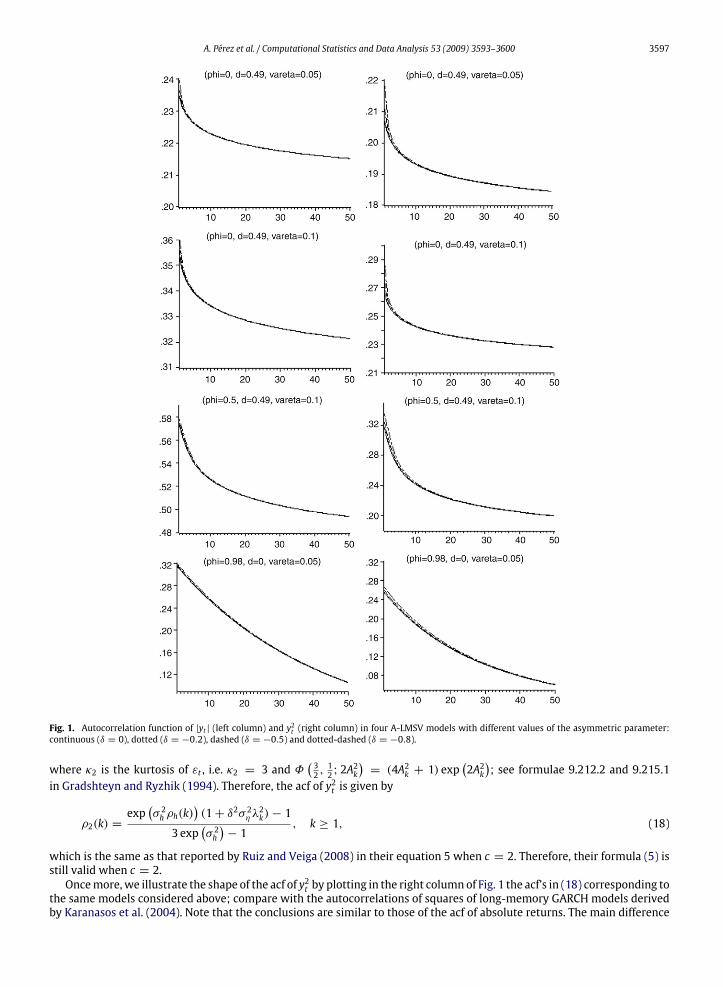
Note that (17) is the correct expression of the autocorrelations of absolute returns in A-LMSV(1, d, 0)models and correctsexpression (5) with c = 1 of Ruiz and Veiga (2008).Given that it is not easy to derive from (17) any conclusion about the shape of the acf of |yt |, the first column of Fig. 1

plots this acf for the same models chosen in Ruiz and Veiga (2008), namely {φ = 0, d = 0.49, σ 2η = 0.05}, {φ = 0, d =0.49, σ 2η = 0.1}, {φ = 0.5, d = 0.49, σ

2η = 0.1} and {φ = 0.98, d = 0, σ

2η = 0.05} and δ = {0,−0.2,−0.5,−0.8}.

Observe that the curves plotted in Fig. 1 for a given model with different values of δ are hardly distinguishable from eachother. Therefore, the presence of leverage effect has a negligible effect on the acf of |yt |. The autocorrelations are nearly thesame regardless of the value of the parameter δ as far as it is negative. Second, we observe that the autocorrelations of |yt |are always positive and decrease monotonically towards zero from the first lag; compare with the conclusions in Ruiz andVeiga (2008) based on the wrong expression of the acf.The acf of squared returns, y2t , is obtained by taking c = 2 in (9), as follows

ρ2(k) =exp

(σ 2h ρh(k)

)exp

(−2A2k

)Φ( 32 ,12 ; 2A

2k

)− 1

κ2 exp(σ 2h)− 1

, k ≥ 1,

A. Pérez et al. / Computational Statistics and Data Analysis 53 (2009) 3593–3600 3597

Fig. 1. Autocorrelation function of |yt | (left column) and y2t (right column) in four A-LMSV models with different values of the asymmetric parameter:continuous (δ = 0), dotted (δ = −0.2), dashed (δ = −0.5) and dotted-dashed (δ = −0.8).

where κ2 is the kurtosis of εt , i.e. κ2 = 3 and Φ( 32 ,12 ; 2A

2k

)= (4A2k + 1) exp

(2A2k

); see formulae 9.212.2 and 9.215.1

in Gradshteyn and Ryzhik (1994). Therefore, the acf of y2t is given by

ρ2(k) =exp

(σ 2h ρh(k)

)(1+ δ2σ 2η λ

2k)− 1

3 exp(σ 2h)− 1

, k ≥ 1, (18)

which is the same as that reported by Ruiz and Veiga (2008) in their equation 5 when c = 2. Therefore, their formula (5) isstill valid when c = 2.Oncemore,we illustrate the shape of the acf of y2t by plotting in the right columnof Fig. 1 the acf’s in (18) corresponding to

the same models considered above; compare with the autocorrelations of squares of long-memory GARCH models derivedby Karanasos et al. (2004). Note that the conclusions are similar to those of the acf of absolute returns. The main difference

3598 A. Pérez et al. / Computational Statistics and Data Analysis 53 (2009) 3593–3600

Fig. 2. Differences between the first order autocorrelations of absolute and squared returns as a function of the correlation between εt and ηt+1 in fourA-LMSV models.

is that the autocorrelations of y2t are systematically smaller than those of |yt |. This phenomenon is known as the Taylor effectin deference to Taylor (1986), who provided extensive empirical evidence on this characteristic of the autocorrelations. Tohave a clearer picture of this effect in A-LMSV(1, d, 0) models, Fig. 2 plots, for the same four models mentioned above, thedifference between the first order autocorrelations of absolute and squared observations as a function of the asymmetryparameter, δ. This figure shows that these differences are all positive, as postulated by the Taylor effect, and they reach theirmaximum when there is no leverage effect (δ = 0) and slightly decrease with the absolute value of δ.

4. Conclusions

In this note, we extend the results of Ruiz and Veiga (2008) by deriving the autocorrelations of powers of absolute returnsand their cross-correlations with the returns themselves, for any value of the power parameter. These functions allow usto have a richer characterization of the dynamics of LMSV models with leverage effect. We also correct a mistake in theexpression of the acf of absolute returns given by Ruiz and Veiga (2008) and, consequently, obtain different conclusions onthe shape of this acf and on the Taylor effect.

Acknowledgments

We acknowledge financial support from the Spanish Government, project SEJ2006-03919. The research of A. Pérezwas also supported by Junta de Castilla y León, projects VA092A08 and VA027A08. We are very grateful to the editorE. Kontoghiorghes and two anonymous referees for their comments.

Appendix

Proposition 1. If(εη

)∼ N

[(00

),

(1 δσηδση σ 2η

)],

then for any finite real number a we have that

E[|ε|c exp(aη)] = 2−c/20(c + 1)0( c2 + 1

) exp(a2σ 2η (1− δ2)2

)Φ

(c + 12

,12;a2σ 2η δ

2

2

), (19)

whereΦ(·, ·; ·) is the degenerate hypergeometric function.

A. Pérez et al. / Computational Statistics and Data Analysis 53 (2009) 3593–3600 3599

Proof. From the law of iterated expectations we have that:

E[|ε|c exp(aη)] = E(|ε|cE[exp(aη)|ε]

). (20)

Since the conditional distribution of η given ε is N(σηδε, σ 2η (1 − δ2)), using the properties of the log-normal distribution,

it turns out that

E[exp(aη)|ε] = exp(aσηδε) exp

(a2σ 2η (1− δ

2)

2

).

Consequently, plugging this expression into Eq. (20), we have

E[|ε|c exp(aη)] = exp

(a2σ 2η (1− δ

2)

2

)E[|ε|c exp(aσηδε)]. (21)

Finally, the expectation on the right-hand side of (21) is given by:

E[|ε|c exp(aσηδε)

]=

1√2π

∫∞

−∞

|ε|c exp(−ε2

2+ aσηδε

)dε

=1√2π

[∫∞

0εc exp

(−ε2

2+ aσηδε

)dε +

∫∞

0εc exp

(−ε2

2− aσηδε

)dε]

=1√2π0(c + 1) exp

(a2σ 2η δ

2

4

)[D−(c+1)(−aσηδ)+ D−(c+1)(aσηδ)], (22)

where D·(·) is the parabolic cylinder function; see formula 3.462.1 in Gradshteyn and Ryzhik (1994). Now, using formula9.240 in Gradshteyn and Ryzhik (1994), it can be proved that

D−(c+1)(−aσηδ)+ D−(c+1)(aσηδ) =2−c/2√2π

0( c2 + 1

) exp(−a2σ 2η δ24

)Φ

(c + 12

,12;a2σ 2η δ

2

2

).

Then, replacing this expression into Eq. (22) it turns out that

E[|ε|c exp(aσηδε)

]= 2−c/2

0(c + 1)0( c2 + 1

)Φ ( c + 12

,12;a2σ 2η δ

2

2

),

and putting back this value into (21) the result in (19) comes up. �

Proposition 2. If(εη

)∼ N

[(00

),

(1 δσηδση σ 2η

)],

then for any finite real number a we have that

E[ε exp(aη)] = aδση exp

(a2σ 2η2

). (23)

Proof. The conditional distribution of η given ε is N(σηδε, σ 2η (1 − δ2)). Therefore by the law of iterated expectations and

the properties of the log-normal distribution, we obtained the following result

E[ε exp (aη)] = E [εE (exp (aη) |ε)]

= exp

{a2σ 2η (1− δ

2)

2

}E[ε exp(aδσηε)]. (24)

The expectation on the right-hand side of (24) is given by

E[ε exp(a δσηε

)] =

1√2π

∫∞

−∞

ε exp(−ε2

2+ aδσηε

)dε

= aδση exp

(a2δ2σ 2η2

); (25)

see formula 3.462.6 in Gradshteyn and Ryzhik (1994).Finally, replacing (25) into (24), the result in (23) is obtained. �

3600 A. Pérez et al. / Computational Statistics and Data Analysis 53 (2009) 3593–3600

References

Demos, A., 2002. Moments and dynamic structure of a time varying parameter stochastic volatility in mean model. Econometrics Journal 5, 345–357.Franq, C., Zakoïan, J., 2008. Deriving the autocovariances of powers of markov-switching GARCH models, with applications to statistical inference.Computational Statistics & Data Analysis 52 (4), 3027–3046.

Ghysels, E., Harvey, A., Renault, E., 1996. Stochastic volatility. In: Rao, C.R., Maddala, G. (Eds.), Statistical Methods in Finance. North-Holland, Amsterdam,pp. 119–191.

Gradshteyn, I., Ryzhik, I., 1994. Table of Integrals, Series and Products. Academic Press.Harvey, A., Shephard, N., 1996. Estimation of an asymmetric stochastic volatility model for asset returns. Journal of Business and Economic Statistics 14,429–434.

Harvey, A.C., 1998. Long-memory in stochastic volatility. In: Knight, J., Satchell, S. (Eds.), Forecasting Volatility in Financial Markets. Butterworth-Heinemann, London.

He, C., Teräsvirta, T., Malmsten, H., 2002. Fourth moment structure of a family of first-order exponential GARCHmodels. Econometric Theory 18, 868–885.Hosking, J., 1981. Fractional differencing. Biometrika 68, 165–176.Karanasos, M., Kim, J., 2003. Moments of the ARMA-EGARCH model. Econometrics Journal 6 (1), 146–166.Karanasos, M., Kim, J., 2006. A re-examination of the asymmetric power ARCH model. Journal of Empirical Finance 13, 113–128.Karanasos, M., Psaradakis, Z., Sola, M., 2004. On the autocorrelation properties of long-memory GARCH processes. Journal of Time Series Analysis 25 (2),265–281.

Nakajima, J., Omori, Y., 2008. Leverage, heavy-tails and correlated jumps in stochastic volatility models. Computational Statistics & Data Analysis,doi:10.1016/j.csda.2008.03.015.

Ruiz, E., Veiga, H., 2008. Modelling long-memory volatilities with leverage effect: A-LMSV versus FIEGARCH. Computational Statistics & Data Analysis 52(6), 2846–2862.

So, M., Lam, K., Li, W., 1997. An empirical study of volatility in seven southeast asian stock markets using ARV models. Journal of Business Finance &Accounting 24 (2), 261–275.

Takahashi, M., Omori, Y., Watanabe, T., 2008. Estimating stochastic volatility models using daily returns and realized volatility simultaneously.Computational Statistics & Data Analysis, doi:10.1016/j.csda.2008.07.39.

Taylor, S., 1986. Modelling Financial Time Series. Wiley: New York.Taylor, S., 2005. Asset Price Dynamics, Volatility and Prediction. Princeton University Press.