A NOTE ON OPTIMAL INFERENCE IN THE LINEAR IV MODEL

By

Donald W. K. Andrews, Vadim Marmer, and Zhengfei Yu

January 2017

COWLES FOUNDATION DISCUSSION PAPER NO. 2073

COWLES FOUNDATION FOR RESEARCH IN ECONOMICS YALE UNIVERSITY

Box 208281 New Haven, Connecticut 06520-8281

http://cowles.yale.edu/

A Note on

Optimal Inference

in the Linear IV Model

Donald W. K. Andrews

Cowles Foundation

Yale University

Vadim Marmer

Vancouver School of Economics

University of British Columbia

Zhengfei Yu

Faculty of Humanities and Social Sciences

University of Tsukuba

October 23, 2015

Revised: January 30, 2017

Andrews gratefully acknowledges the research support of the National Science Foundation via grant numberSES-1355504. Marmer gratefully acknowledges the research support of the SSHRC via grant numbers 410-2010-1394and 435-2013-0331.

Abstract

This paper considers tests and condence sets (CSs) concerning the coe¢ cient on the endogenous vari-

able in the linear IV regression model with homoskedastic normal errors and one right-hand side endogenous

variable. The paper derives a nite-sample lower bound function for the probability that a CS constructed

using a two-sided invariant similar test has innite length and shows numerically that the conditional likeli-

hood ratio (CLR) CS of Moreira (2003) is not always very closeto this lower bound function. This implies

that the CLR test is not always very close to the two-sided asymptotically-e¢ cient (AE) power envelope for

invariant similar tests of Andrews, Moreira, and Stock (2006) (AMS).

On the other hand, the paper establishes the nite-sample optimality of the CLR test when the correlation

between the structural and reduced-form errors, or between the two reduced-form errors, goes to 1 or -1 and

other parameters are held constant, where optimality means achievement of the two-sided AE power envelope

of AMS. These results cover the full range of (non-zero) IV strength.

The paper investigates in detail scenarios in which the CLR test is not on the two-sided AE power

envelope of AMS. Also, the paper shows via theory and numerical work that the CLR test is close to having

greatest average power, where the average is over a grid of concentration parameter values and over pairs

alternative hypothesis values of the parameter of interest, uniformly over pairs of alternative hypothesis

values and uniformly over the correlation between the structural and reduced-form errors.

The paper concludes that, although the CLR test is not always very close to the two-sided AE power

envelope of AMS, CLR tests and CSs have very good overall properties.

Keywords: Conditional likelihood ratio test, condence interval, innite length, linear instrumental

variables, optimal test, weighted average power, similar test.

JEL Classication Numbers: C12, C36.

1 Introduction

The linear instrumental variables (IV) regression model is one of the most widely used models

in economics. It has been widely studied and considerable e¤ort has been made to develop good

estimation and inference methods for it. In particular, following the recognition that standard two

stage least squares t tests and condence sets (CSs) can perform quite poorly under weak IVs

(see Dufour (1997), Staiger and Stock (1997), and references therein), inference procedures that

are robust to weak IVs have been developed, e.g., see Kleibergen (2002) and Moreira (2003, 2009).

The focus has been on models with one right-hand side (rhs) endogenous variable, because this

arises most frequently in applications, and on over-identied models, because Anderson and Rubin

(1949) (AR) tests and CSs are robust to weak IVs and perform very well in exactly-identied

models.

Andrews, Moreira, and Stock (2006) (AMS) develop a nite-sample two-sided AE power en-

velope for invariant similar tests concerning the coe¢ cient on the rhs endogenous variable in the

linear IV model under homoskedastic normal errors and known reduced-form variance matrix. They

show via numerical simulations that the conditional likelihood ratio (CLR) test of Moreira (2003)

has power that is essentially (i.e., up to simulation error) on the power envelope. Chernozhukov,

Hansen, and Jansson (2009) (CHJ) show that this power envelope also applies to non-invariant

tests provided the envelope is for power averaged over certain direction vectors in a unit sphere.

CHJ also shows that the invariant similar tests that generate the two-sided AE power envelope

are -admissible and d-admissible. Mikusheva (2010) provides approximate optimality results for

CLR-based CSs that utilize the testing results in AMS. Chamberlain (2007), Andrews, Moreira,

and Stock (2008), and Hillier (2009) provide related results.

It is shown in Dufour (1997) that any CS with correct size 1 must have positive probabilityof having innite length at every point in the parameter space. The AR and CLR CSs have this

property. In fact, simulation results show that in some over-identied contexts the AR CS has

a lower probability of having an innite length than the CLR CS does. For example, consider a

model with one rhs endogenous variable, k IVs, a concentration parameter v (which is a measure

of the strength of the IVs), homoskedastic normal errors, a correlation uv between the structural-

equation error and the reduced-form error (for the rst-stage equation) equal to zero, and no

covariates. When (k; v) equals (2; 7); (5; 12); (10; 15); (20; 20); and (40; 20); the di¤erences between

the probabilities that the 95% CLR and AR CSs have innite length are :016; :029; :037; :044;

and :049; respectively.1 In fact, one obtains positive di¤erences for all combinations of (k; v) for

k = 2; 5; 10; 20; 40 and v = 1; 5; 10; 15; 20: Hence, in these over-identied scenarios the AR CS1See Table SM-I in the Supplemental Material.

1

outperforms the CLR CS in terms of its innite-length behavior, which is an important property

for CSs. Similarly, one obtains positive (but smaller) di¤erences also when uv = :3 for the same

range of (k; v) values. On the other hand, for uv = :5; :7; and :9; the di¤erences are negative over

the same range of (k; v) values.

The AR and CLR CSs are based on inverting AR and CLR tests that fall into the class of

invariant similar tests considered in AMS. Hence, the simulation results for uv = :0 and :3 raise

the question: how can these results be reconciled with the near optimal CLR test and CS results

described above? In this paper, we answer this question and related questions concerning the

optimality of the CLR test and CS.

The contributions of the paper are as follows. First, the paper shows that the probability that

an invariant similar CS has innite length for a xed true parameter value equals one minus the

power against of the test used to construct the CS as the null value 0 goes to 1 or 1: Thisleads to explicit formulae for the probabilities that the AR and CLR CSs have innite length.

Second, the paper uses the rst result to determine a nite-sample lower bound function on

the probabilities that a CS has innite length for CSs based on invariant similar tests. The lower

bound function is found to be very simple. It is a function only of juvj; v; and k: These resultsallow one to compare the probabilities that the AR and CLR CSs have innite length with the

lower bound.

Third, simulation results show that the AR and CLR CSs are not always close to the lower

bound. This is not surprising for the AR CS, but it is surprising for the CLR CS in light of the

AMS results. The probabilities that the CLR CS has innite length are found to be o¤ the lower

bound function by a magnitude that is decreasing in juvj; increasing in k; and are maximized overv at values that correspond to somewhat weak IVs, but not irrelevant IVs. For uv = 0; the paper

shows (analytically) that the AR test achieves the lower bound function. Hence, for uv = 0; the

probabilities that the CLR CS has innite length exceed the lower bound by the same amounts as

reported above for the di¤erence between the innite length probabilities of the CLR and AR CSs

for several (k; v) values. On the other hand, for values of juvj :7; the CLR CS has probabilities

of having innite length that are close to the lower bound function, :010 or less and typically much

less, for all (k; v) combinations considered. For values of juvj :7; the AR CS has probabilities

of having innite length that are often far from the lower bound. For juvj = :9 and certain values

of v; they are as large as :084; :196; :280; :353; and :422 for k = 2; 5; 10; 20; and 40; respectively.2

Fourth, the paper derives new optimality properties of the CLR test when uv ! 1 or ! 1with other parameters xed at any values (with non-zero concentration parameter), where

2See Table SM-I in the SM.

2

denotes the correlation between the reduced-form errors. Optimality here is in the class of invariant

similar tests or similar tests and employs the two-sided AE power envelope of AMS. These results

are consistent with the numerical results that show that the CLR test is very close to the power

envelope when juvj is large.Fifth, we simulate power di¤erences (PDs) between the two-sided AE power envelope of AMS

and the power of the CLR test for a xed alternative value and a range of nite null values

0 (rather than the PDs as 0 ! 1 discussed above). These PDs are equivalent to the false

coverage probability di¤erences between the CLR CS and the corresponding infeasible optimal

CS for a xed true value at incorrect values 0: We consider a wide range of (0; v; uv; k)

values. The maximum (over 0 and v values) PDs range between [:016; :061] over the (uv; k)

values considered. On the other hand, the average (over 0 and values) PDs only range between

[:002; :016]: This indicates that, although there are some (0; ) values at which the CLR test is

noticeably o¤ the power envelope, on average the CLR tests power is not far from the power

envelope. The maximum PDs over (0; ) are found to increase in k and decrease in juvj: Thev values at which the maxima are obtained are found to (weakly) increase with k and decrease

in juvj: The j0j values at which the maxima are obtained are found to be independent of k anddecrease in juvj:

Sixth, the paper considers a weighted average power (WAP) envelope with a uniform weight

function over a grid of concentration parameter values v and the same two-point AE weight

function over (; ) as in AMS. We refer to this as the WAP2 envelope. We determine numerically

how close the power of the CLR test is to the WAP2 envelope. We nd that the di¤erence between

the WAP2 envelope and the average power of the CLR test is in the range of [:001; :007] over all

of the (0; ; uv; k) values that we consider. Hence, the average power of the CLR test is quite

close to the WAP2 envelope.

Other papers in the literature that consider WAP include Wald (1943), Andrews and Ploberger

(1994), Andrews (1998), Moreira and Moreira (2013), Elliott, Müller, and Watson (2015), and

papers referenced above. The WAP2 envelope considered here is closest to the WAP envelopes

in Wald (1943), AMS, and CHJ because the other papers listed put a weight function over all of

the parameters in the alternative hypothesis, which yields a single weighted alternative density. In

contrast, the WAP2 envelope, Wald (1943), AMS, and CHJ consider a family of weight functions

over disjoint sets of parameters in the alternative hypothesis, which yields a WAP envelope.

In conclusion, based on our ndings, we recommend use of the CLR test and CS. More specif-

ically, we recommend using heteroskedasticity-robust versions of these procedures that have the

same asymptotic properties as these procedures under homoskedasticity. For example, such tests

3

are given in Andrews, Moreira, and Stock (2004) and Andrews and Guggenberger (2015). The

CLR CS has higher probability of having innite length than the AR CS in some scenarios, and

the CLR test is not a UMP two-sided invariant similar test. But, no such UMP test exists and the

CLR CS is close to the two-sided AE power envelope for invariant similar tests when juvj is notclose to zero and is close to the WAP2 envelope for all values of juvj:

Finally, we point out that the results of this paper illustrate a point that applies more generally

than in the linear IV model. In weak identication scenarios, where CSs may have innite length

(or may be bounded only due to bounds on the parameter space), good test performance at a priori

implausible parameter values is important for good CS performance at plausible parameter values.

More specically, the probability under an a priori plausible parameter value that a CS has

innite length depends on the power of the test used to construct the CS against when the null

value j0j is arbitrarily large, which may be an a priori implausible null value.For the computation of CLR CSs, see Mikusheva (2010). For a formula for the power of the

CLR test, see Hillier (2009).

The paper is organized as follows. Section 2 species the model. Section 3 denes the class

of invariant similar tests. Section 4 provides a formula for the probability that a CS has innite

length. Section 5 derives a lower bound on the probability that a CS constructed using two-sided

invariant similar tests has innite length. Section 6 reports di¤erences between the probability

that the CLR CS has innite length and the lower bound derived in the previous section. Section

7 proves the optimality results for the CLR test described above. Section 8 reports di¤erences

between the power of CLR tests and the two-sided AE power bound of AMS for a wide range of

parameter congurations. Section 9 provides comparisons of the power of the CLR test to the

WAP2 power envelope described above. Proofs and additional theoretical and numerical results

are given in the Supplemental Material (SM).

2 Model

We consider the same model as in Andrews, Moreira, and Stock (2004, 2006) (AMS04,

AMS) but, for simplicity and without loss of generality (wlog), without any exogenous variables.

The model has one rhs endogenous variable, k instrumental variables (IVs), and normal errors

with known reduced-form error variance matrix. The model consists of a structural equation and

a reduced-form equation:

y1 = y2 + u and y2 = Z + v2; (2.1)

4

where y1; y2 2 Rn and Z 2 Rnk are observed variables; u; v2 2 Rn are unobserved errors; and

2 R and 2 Rk are unknown parameters. The IV matrix Z is xed (i.e., non-stochastic) and

has full column rank k: The n 2 matrix of errors [u:v2] is i.i.d. across rows with each row havinga mean zero bivariate normal distribution.

The two corresponding reduced-form equations are

Y := [y1 :y2] := [Z + v1 :Z + v2] = Za0 + V; where

V := [v1 : v2] = [u+ v2 : v2]; and a := (; 1)0: (2.2)

The distribution of Y 2 Rn2 is multivariate normal with mean matrix Za0; independence acrossrows, and reduced-form variance matrix 2 R22 for each row. For the purposes of obtaining

exact nite-sample results, we suppose is known. As in AMS, asymptotic results for unknown

and weak IVs are the same as the exact results with known : The parameter space for = (; 0)0

is Rk+1:

We are interested in tests of the null hypothesis H0 : = 0 and CSs for :

As shown in AMS, Z 0Y is a su¢ cient statistic for (; 0)0: As in Moreira (2003) and AMS, we

consider a one-to-one transformation [S : T ] of Z 0Y :

S := (Z 0Z)1=2Z 0Y b0 (b00b0)1=2 N(c(0;) ; Ik) and

T := (Z 0Z)1=2Z 0Y 1a0 (a001a0)1=2 N(d(0;) ; Ik); where

b0 := (1;0)0; a0 := (0; 1)0; := (Z 0Z)1=2 2 Rk;

c(0;) := ( 0) (b00b0)1=2 2 R;

d(0;) := b0b0 (b00b0)1=2 det()1=2 2 R; and b = (1;)0: (2.3)

As dened, S and T are independent. Note that S and T depend on the null hypothesis value 0:

3 Invariant Similar Tests

As in Hillier (1984) and AMS, we consider tests that are invariant to orthonormal transfor-

mations of [S : T ]; i.e., [S : T ] ! [FS : FT ] for a k k orthogonal matrix F: The 2 2 matrix Qis a maximal invariant, where

Q = [S:T ]0[S:T ] =

24 S0S S0T

S0T T 0T

35 =24 QS QST

QST QT

35 and Q1 =

0@ S0S

S0T

1A =

0@ QS

QST

1A ; (3.1)

5

e.g., see Theorem 1 of AMS. Note that Q1 is the rst column of Q and the matrix Q depends on

the null value 0:

The statistic Q has a non-central Wishart distribution because [S :T ] is a multivariate normal

matrix that has independent rows and common covariance matrix across rows. The distribution of

Q depends on only through the scalar

:= 0Z 0Z 0: (3.2)

Leading examples of invariant identication-robust tests in the literature include the AR test,

the LM test of Kleibergen (2002) and Moreira (2009), and the CLR test of Moreira (2003). The

latter test depends on the standard LR test statistic coupled with a conditional critical value

that depends on QT . The LR, LM, and AR test statistics are

LR :=1

2

QS QT +

q(QS QT )2 + 4Q2ST

;

LM := Q2ST =QT = (S0T )2=T 0T; and AR := QS=k = S0S=k: (3.3)

The critical values for the LM and AR tests are 21;1 and 2k;1=k; respectively, where

2m;1

denotes the 1 quantile of the 2 distribution with m degrees of freedom.

A test based on the maximal invariant Q is similar if its null rejection rate does not depend

on the parameter that determines the strength of the IVs Z: As in Moreira (2003), the class of

invariant similar tests is specied as follows. Let the [0; 1]-valued statistic (Q) denote a (possibly

randomized) test that depends on the maximal invariant Q: An invariant test (Q) is similar with

signicance level if and only if E0((Q)jQT = qT ) = for almost all qT > 0 (with respect to

Lebesgue measure), where E0(jQT = qT ) denotes conditional expectation given QT = qT when

= 0 (which does not depend on ):

The CLR test rejects the null hypothesis when

LR > LR;(QT ); (3.4)

where LR;(QT ) is dened to satisfy P0(LR > LR;(QT )jQT = qT ) = and the conditional

distribution of Q1 given QT is specied in AMS and in (11.3) in the SM.

The invariance condition discussed above is a rotational invariance condition. In some cases,

we also consider a sign invariance condition. A test that depends on [S : T ] is sign invariant if it is

invariant to the transformation [S : T ] ! [S : T ]: A rotation invariant test is also sign invariantif it depends on QST only through jQST j: Tests that are sign invariant are two-sided tests. In fact,

6

AMS shows that the two-sided AE power envelope is identical to the power envelope generated by

sign and rotation invariant tests, see (4.11) in AMS.

For simplicity, we will use the term invariant test to mean a rotation invariant test and the term

sign and rotation invariant test to describe a test that satises both invariance conditions.

The paper also provides some results that apply to tests that satisfy no invariance properties.

A test ([S : T ]) (that is not necessarily invariant) is similar with signicance level if and only if

E0(([S : T ])jT = t) = for almost all t (with respect to Lebesgue measure), where E0(jT = t)

denotes conditional expectation given T = t when = 0 (which does not depend on ); see

Moreira (2009).

4 Probability That a Condence Set Has Innite Length

In this section, we show that the probability that a condence set (CS) has innite length is

given by one minus the power of the test used to construct the CS as the null value 0 of the test

goes to1 or 1: This provides motivation for interest in the power of tests as 0 ! 1: It showswhy high power against distant null hypotheses is highly desirable.

We sometimes make the dependence of Q; S; and T on Y and 0 explicit and write

Q = Q0(Y ) = [S0(Y ) : T0(Y )]0[S0(Y ) : T0(Y )]: (4.1)

We denote the (1; 1); (1; 2); and (2; 2) elements of Q0(Y ) by QS;0(Y ); QST;0(Y ); and QT;0(Y );

respectively.

Let

(Q0(Y )) = 1(T (Q0(Y )) > cv(QT0(Y ))) (4.2)

be a (nonrandomized) invariant similar level test for testing H0 : = 0 for xed known ;

where T (Q0(Y )) is a test statistic and cv(QT0(Y )) is a (possibly data-dependent) critical value.Examples include the AR, LM, and CLR tests in (3.3). Let CS be the level 1 CS correspondingto : That is,

CS(Y ) = f0 : (Q0(Y )) = 0g: (4.3)

We say CS(Y ) has right (or left) innite length, which we denote by RLength(CS(Y )) =1(or LLength(CS(Y )) =1), if

9K(Y ) <1 such that 2 CS(Y ) 8 K(Y ) (or 8 K(Y )): (4.4)

7

We say CS(Y ) has innite length, which we denote by Length(CS(Y )) =1; if it has right andleft innite lengths. A CS with innite length contains a set of the form (1;K1(Y ))[(K2(Y );1)for some 1 < K1(Y ) K2(Y ) <1:

Let P;;() denote probability for events determined by Y when Y has a multivariate normaldistribution with means matrix [ : ] 2 R2k; independence across rows, and variance matrix for each row. Let P;0;;() denote probability for events determined by Q when Q := [S : T ]

0[S :

T ] and [S : T ] has the multivariate normal distribution in (2.3) with = and = 0: In this

case, Q has a noncentral Wishart distribution whose density is given in (11.2) in the SM.

For xed true value and reduced-form variance matrix ; let denote the corresponding

structural variance matrix of each row of [u : v2]: Let uv denote the correlation between the

structural and reduced-form errors, i.e., the correlation corresponding to : Some calculations

show that

uv =!12 !22

(!21 2!12 + !222)1=2!2and

=

24 2u uvuv

uvuv 2v

35 =24 !21 2!12 + !222 !12 !22

!12 !22 !22

35 ; (4.5)

where !21; !22; and !12 denote the (1; 1); (2; 2); and (1; 2) elements of ; respectively, see (11.9) in

the SM.

It is shown in Lemma 15.1 in the SM that the limit as 0 ! 1 of Q0(Y ) is

Q1(Y ) :=

24 e02Y0PZY e2 12v e02Y

0PZY 1e1 (1

2uv)

1=2uv

e02Y0PZY

1e1 (12uv)

1=2uv

e011Y 0PZY

1e1 (1 2uv)2u

35 ; (4.6)

where PZ := Z(Z 0Z)1Z 0; e1 := (1; 0)0; and e2 := (0; 1)0: Let QT;1(Y ) denote the (2; 2) element

of Q1(Y ): It is also shown in Lemma 15.1 in the SM that Q1(Y ) has a noncentral Wishart

distribution with means matrix (1=v; uv=(v(1 2uv)1=2)) 2 Rk2 and identity variance

matrix.3

Theorem 4.1 Suppose CS(Y ) is a CS based on invariant level tests (Q0(Y )) whose test

statistic and critical value functions, T (q) and cv(qT ); respectively, are continuous at all positivedenite 2 2 matrices q and positive constants qT ; P;;(T (Qc(Y )) = cv(QT;c(Y ))) = 0 for

c = +1 in parts (a) and (c) below and c = 1 in part (b) below. Then, for all (; ;);

(a) P;;(RLength(CS(Y )) =1) = 1 lim0!1 P;0;;((Q) = 1);

3The density of this distribution is given in (11.4) in the SM.

8

(b) P;;(LLength(CS(Y )) =1) = 1 lim0!1 P;0;;((Q) = 1); and

(c) if the tests are sign invariant, i.e., T (Q) depends on QST only through jQST j; thenP;;(Length(CS(Y )) =1) = 1 lim0!1 P;0;;((Q) = 1):

Comments. (i). For the AR, LM, and LR tests, the continuity conditions on T (q) and cv(qT )hold given their simple functional forms in (3.3) using the assumption that qT > 0 for the LM

statistic and using the continuity of LR;(qT ); which holds by the argument in the proof of Thm.

10.1 in Andrews and Guggenberger (2016). We have P;;(T (Q1(Y )) = cv(QT;1(Y ))) = 0 for

the AR and LM tests because cv(QT;1(Y )) is a constant and T (Q1(Y )) is absolutely continuouswith respect to Lebesgue measure. For the CLR test, P;;(T (Q1(Y )) = cv(QT;1(Y ))) = 0 by

the argument given in the proof of Theorem 5.4 in the SM. The AR, LM, and CLR test statistics are

sign invariant. Hence, parts (a)-(c) of Theorem 4.1 apply to these tests. Theorem 5.4(a)-(c) below

provides formulae for the quantities lim0!1 P;0;;((Q) = 1); which appear in Theorem 4.1,

for the AR, LM, and CLR tests.

(ii). Comment (iii) to Theorem 5.2 below provides a lower bound on 1lim0!1 P;0;;((Q)

= 1) over all sign and rotation invariant similar level tests. Combining this with Theorem 4.1(c)

yields a lower bound on the probability that a CS CS(Y ) based on such tests has Length = 1:The lower bound on the probability that Length = 1 is greater than the lower bound on the

probability that RLength =1 (or that LLength =1) unless uv = 0 (in which case it turns outthat they are equal).

Theorem 12.1 in the SM provides lower bounds on 1 lim0!1 P;0;;((Q) = 1) over all

invariant similar level tests. Combining these with Theorem 4.1(a) and (b) yields lower bounds

on the probabilities that a CS CS(Y ) has RLength = 1 based on 0 ! 1 and LLength = 1based on 0 ! 1:

(iii). The results of Theorem 4.1(a) and (b) also hold for a CS(Y ) that is based on level

tests that are not invariant. Denote such tests by (S0(Y ); T0(Y )) and suppose their test

statistic and critical value functions, T (s; t) and cv(t); respectively, are continuous at all k 2matrices [s : t] and k vectors t and satisfy P;;(T (Sc(Y ); Tc(Y )) = cv(Tc(Y ))) = 0 for c = +1;where S1(Y ) := (Z 0Z)1=2Z 0Y e2=v and T1(Y ) := (Z 0Z)1=2Z 0Y 1e1 (1 2uv)1=2u: Inthis case, P;;(RLength(CS(Y )) = 1) = 1 lim0!1 P;0;;(([S : T ]) = 1) and likewise

with LLength(); 0 ! 1; and c = 1 in place of RLength(); 0 !1; and c = +1:(iv). By Dufour (1997), all CSs for with correct size must have positive probability of

having innite length (assuming is not bounded away from 0). In consequence, expected CS

length, which is a standard measure of the performance of a CS, is innite for all identication-

robust CSs. Due to this, Mikusheva (2010) compares CSs based on their expected truncated

9

lengths for various truncation values. The result of Theorem 5.2 below implies that, for two CSs

where the rhs of Theorem 5.2(c) is smaller for the rst CS than the second, the rst CS has smaller

expected truncated length than the second for su¢ ciently large truncation values.

5 Power Bound as 0! 1

In this section, we provide two-sided AE power bounds for invariant similar tests as 0 ! 1for xed : The power bounds also apply to the larger class of similar tests for which invariance is

not imposed, provided power is averaged over =jjjj vectors using the uniform distribution on

the unit sphere in Rk; as in CHJ.

Using Theorem 4.1, these results are used to obtain bounds on the probabilities that CSs

constructed using sign and rotation invariant similar tests have innite length. They also are used

to obtain bounds on certain average probabilities that similar invariant tests and similar tests have

innite right (or left) length.

This section also determines the power of the AR, LM, and CLR tests as 0 ! 1 and the

probabilities that AR, LM, and CLR CSs have innite length.

5.1 Density of Q as 0! 1

The density of Q := [S : T ]0[S : T ] when [S : T ] has the multivariate normal distribution in (2.3)

only depends on through := 0: Let fQ(q;; 0; ;) denote this density when = :

It is a noncentral Wishart density with means matrix of rank one and identity covariance matrix,

which was rst derived by Anderson (1946, eqn. (6)). An explicit expression for fQ(q;; 0; ;)

is given in (11.2) in the SM.

Now, we determine the limit of the density fQ(q;; 0; ;) as 0 ! 1: Dene

ruv :=uv

(1 2uv)1=2and v := =2v = 0=

2v: (5.1)

Note that v is the concentration parameter, which indexes the strength of the IVs. Let

fQ(q; uv; v) denote the density of Q := [S : T ]0[S : T ] when [S : T ] has a multivariate nor-

mal distribution with means matrix

(1=v; ruv=v) 2 Rk2; (5.2)

all variances equal to one, and all covariances equal to zero. This density also is a noncentral Wishart

density with means matrix of rank one and identity covariance matrix. The density depends on

10

ruv; v; and only through uv and v: An explicit expression for fQ(q; uv; v) is given in (11.4)

in Section 11.1 the SM.

Lemma 5.1 For any xed (; ;); lim0!1 fQ(q;; 0; ;) = fQ(q; uv; v) for all 2 2variance matrices q; where uv and v are dened in (4.5) and (5.1), respectively.

Comment. Lemma 5.1 is proved by showing: lim0!1 c(0;) = 1=v and lim0!1d(0;) = !22!12

!2(!21!22!212)1=2

= uvv(12uv)1=2

; see Lemma 14.1 in the SM. When expressed in

terms of ; the latter limit only depends on uv; u; and v and its functional form is of a

relatively simple multiplicative form.

Let P;0;;() and Puv ;v() denote probabilities under the alternative hypothesis densitiesfQ(q;; 0; ;) and fQ(q; uv; v); respectively, dened above.

5.2 Two-Sided AE Power Bound as 0! 1

AMS provides a two-sided power envelope for invariant similar tests based on maximizing av-

erage power against two points in the alternative hypothesis: (; ) and (2; 2): AMS refers to

this as the two-sided AE power envelope because given one point (; ); the second point (2; 2)

is the unique point such that the test that maximizes average power against these two points is

a two-sided AE e¢ cient test under strong IV asymptotics. This power envelope is a function of

(; ):

Given (; ); the second point (2; 2) satises

2 = 0 d0( 0)

d0 + 2r0( 0)and 2 =

(d0 + 2r0( 0))2

d20; (5.3)

where r0 := e011a0 (a001a0)1=2; see (4.2) of AMS. We let POIS2(Q;0; ; ) denote the

optimal average-power test statistic for testing = 0 against (; ) and (2; 2): Its condi-

tional critical value is denoted by 2;0(QT ): For brevity, the formulas for POIS2(Q;0; ; ) and

2;0(QT ) are given in Section 16 in the SM.

The limit as 0 ! 1 of the POIS2(Q;0; ; ) statistic is shown in (16.6) in the SM to be

POIS2(Q;1; juvj; v) := (Q; uv; v) + (Q;uv; v)

2 2(QT ; juvj; v); where

(Q; uv; v) := exp(v(1 + r2uv)=2)(v(Q; uv))(k2)=4I(k2)=2(pv(Q; uv));

2(QT ; juvj; v) := exp(vr2uv=2)(vr2uvQT )(k2)=4I(k2)=2(pvr2uvQT ); and

(Q; uv) := QS + 2ruvQST + r2uvQT ; (5.4)

11

where Q; QS ; QST ; and QT are dened in (3.1), uv is dened in (4.5), ruv and v are dened in

(5.1), and I() denotes the modied Bessel function of the rst kind of order (e.g., see Comment(ii) to Lemma 3 of AMS for more details regarding I()):

Let 2;1(qT ) denote the conditional critical value of the POIS2(Q;1; juvj; v) test statistic.That is, 2;1(qT ) is dened to satisfy

PQ1jQT (POIS2(Q;1; juvj; v) > 2;1(qT )jqT ) = (5.5)

for all qT 0; where PQ1jQT (jqT ) denotes probability under the null density fQ1jQT (jqT ); which isspecied explicitly in (11.3) in the SM and does not depend on 0:

When uv = 0; the test based on POIS2(Q;1; juvj; v) is the AR test. This follows because(Q; 0) = QS ; (Q; 0; v) is monotone increasing in (Q; 0); and 2(QT ; 0; v) is a constant. Some

intuition for this is that EQST = 0 under the null and limj0j!1EQST = 0 under any xed

alternative when uv = 0:4 In consequence, QST is not useful for distinguishing between H0 and

H1 when j0j ! 1 and uv = 0: Furthermore, it is shown in (12.5) and Theorem 12.1 in the SM

that the AR test is also the best one-sided test as 0 ! +1 and as 0 ! 1:The following theorem shows that the POIS2(Q;1; juvj; v) test provides a two-point average-

power bound as 0 ! 1 for any invariant similar test for any xed (; ) and :

Theorem 5.2 Let f0(Q) : 0 ! 1g be any sequence of invariant similar level tests of

H0 : = 0 for xed known : For xed (; ); (2; 2) dened (5.3), and ; the two-sided AE

power envelope test POIS2(Q;1; juvj; v) dened in (5.4) and (5.5) satises

lim sup (0!1

P;0;;(0(Q) = 1) + P2;0;2;(0(Q) = 1))=2

Puv ;v(POIS2(Q;1; juvj; v) > 2;1(QT ))

= Puv ;v(POIS2(Q;1; juvj; v) > 2;1(QT )):

Comments. (i). The power bound in Theorem 5.2 only depends on (; ); (2; 2); and

through juvj; which is the absolute magnitude of endogeneity under ; and v; which is the

concentration parameter.

(ii). The power bound in Theorem 5.2 is strictly less than one. Hence, it is informative.

(iii). For sign and rotation invariant similar tests 0(Q); the lim sup on the left-hand side in

Theorem 5.2 is the average of two equal quantities.

4We have EQST = ES0ET by independence of S and T; EQST = 0 under H0 because ES = 0; andlimj0j!1EQST = 0 under because ET = d(0;); lim0!1 d(0;)! ruv=v by Lemma 14.1(e) inthe SM, and ruv = 0 when uv = 0:

12

(iv). Theorem 5.2 can be extended to cover sequences of similar tests f0(S; T ) : 0 !1g that satisfy no invariance properties, using the proof of Theorem 1 in CHJ. In this case,

the left-hand side (lhs) probabilities in Theorem 5.2 depend on or, equivalently (; =jjjj);rather than just : In this case, Theorem 5.2 holds with P;0;;(0(Q) = 1) replaced byRP;;=jj jj;(0(S; T ) = 1)dUnif(=jjjj) and analogously for the term that depends on

(2; 2); where P;;=jj jj;() denotes probability under (; ; =jjjj;) and Unif() de-notes the uniform measure on the unit sphere in Rk:

5.3 Lower Bound on the Probability That a CS Has Innite Length

Next, we combine Theorems 4.1 and 5.2 to provide a lower bound on the probability that a

sign and rotation invariant similar CS has innite length. The same lower bound applies to the

average probability over (; ) and (2; ) that a rotation invariant similar CS has right (left)

innite length. For a similar CS with no invariance properties, the same lower bound applies to a

di¤erent average probability that the CS has right (left) innite length.

Let P;;() denote probability for events determined by (Z0Z)1=2Z 0Y that depend on only

through ; such as events that are determined by a CS based on invariant tests.

Corollary 5.3 Suppose CS(Y ) is a CS based on invariant similar level tests (Q0(Y )) that

satisfy the continuity condition in Theorem 4.1. (a) For any xed (; ;);

(P;;(RLength(CS(Y )) =1) + P2;2;(RLength(CS(Y )) =1))=2

1 Puv ;v(POIS2(Q;1; juvj; v) > 2;1(QT )) and

(P;;(LLength(CS(Y )) =1) + P2;2;(LLength(CS(Y )) =1)

1 Puv ;v(POIS2(Q;1; juvj; v) > 2;1(QT )):

(b) If the tests (Q0(Y )) also are sign invariant, then for any xed (; ;);

P;;(Length(CS(Y )) =1) 1 Puv ;v(POIS2(Q;1; juvj; v) > 2;1(QT )):

Comments. (i). All three lower bounds in Corollary 5.3 are the same. The di¤erent parts of

Corollary 5.3 specify di¤erent probabilities or average probabilities that have this lower bound.

(ii). Corollary 5.3(a) also holds for a similar CS that does not satisfy any invariance properties.

In this case, P;;(RLength(CS(Y )) =1) is replaced byRP;;=jj jj;(RLength(CS(Y )) =

1)dUnif(=jjjj) and analogously for the other three lhs terms that depend on LLength(CS(Y ))

13

and/or (2; 2): This holds provided the similar level tests (S0(Y ); T0(Y )) that dene the

CS satisfy the conditions in Comment (iii) to Theorem 4.1.

5.4 Power of the AR, LM, and CLR Tests as 0! 1

Here, we provide the power of the AR, LM, and CLR tests as 0 ! 1 for xed (;):

Theorem 5.4 For xed true (; ;); the AR, LM, and CLR tests satisfy

(a) lim0!1 P;0;;(AR > 2k;1=k) = Puv ;v(AR > 2k;1=k) = P (2k(v) > 2k;1);

(b) lim0!1 P;0;;(LM > 21;1) = Puv ;v(LM > 21;1); and

(c) lim0!1 P;0;;(LR > LR;(QT )) = Puv ;v(LR > LR;(QT ));

where AR; LM; and LR are dened as functions of Q in (3.3), 2m;1 is the 1 quantile of the2m distribution, and 2m(v) is a noncentral

2m random variable with noncentrality parameter v:

Comment. By Theorem 4.1(c), Theorem 5.4 provides the probabilities that the AR, LM, and

CLR CSs have innite length when the true parameters are (; ;): These probabilities depend

only on (juvj; v): For the AR CS, they only depend on v:

6 Comparisons of Probabilities That Condence Sets Have

Innite Length

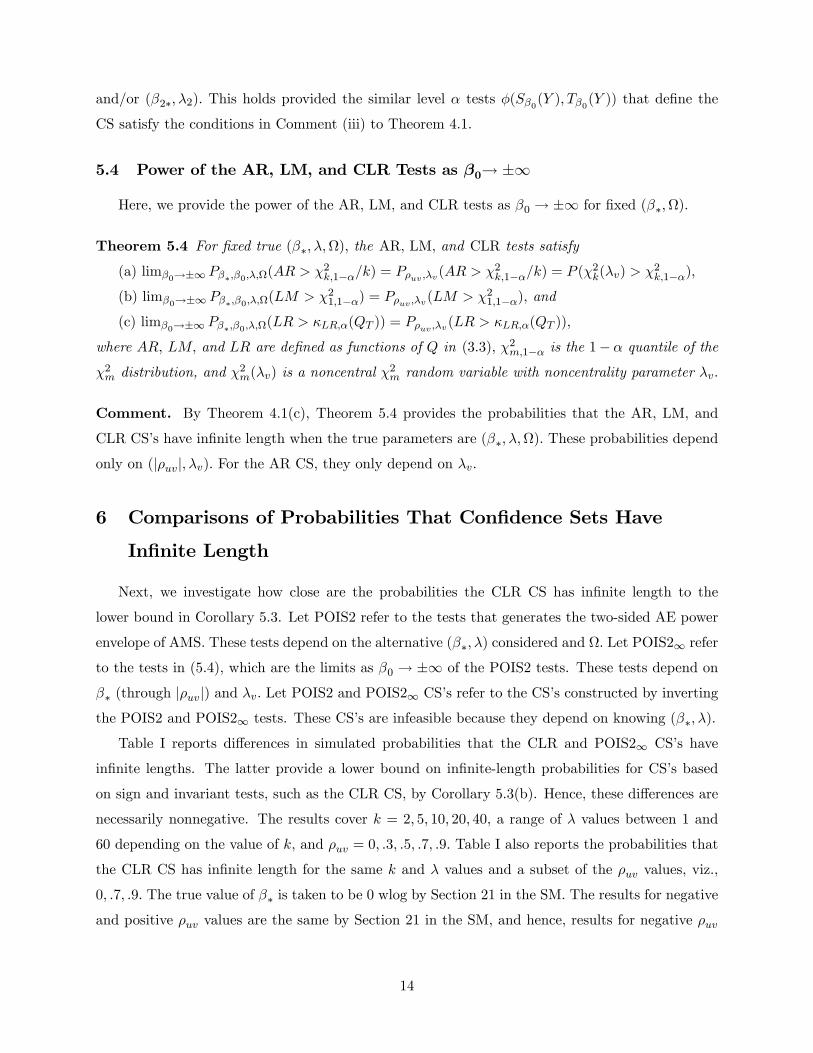
Next, we investigate how close are the probabilities the CLR CS has innite length to the

lower bound in Corollary 5.3. Let POIS2 refer to the tests that generates the two-sided AE power

envelope of AMS. These tests depend on the alternative (; ) considered and : Let POIS21 refer

to the tests in (5.4), which are the limits as 0 ! 1 of the POIS2 tests. These tests depend on

(through juvj) and v: Let POIS2 and POIS21 CSs refer to the CSs constructed by inverting

the POIS2 and POIS21 tests. These CSs are infeasible because they depend on knowing (; ):

Table I reports di¤erences in simulated probabilities that the CLR and POIS21 CSs have

innite lengths. The latter provide a lower bound on innite-length probabilities for CSs based

on sign and invariant tests, such as the CLR CS, by Corollary 5.3(b). Hence, these di¤erences are

necessarily nonnegative. The results cover k = 2; 5; 10; 20; 40; a range of values between 1 and

60 depending on the value of k; and uv = 0; :3; :5; :7; :9: Table I also reports the probabilities that

the CLR CS has innite length for the same k and values and a subset of the uv values, viz.,

0; :7; :9: The true value of is taken to be 0 wlog by Section 21 in the SM. The results for negative

and positive uv values are the same by Section 21 in the SM, and hence, results for negative uv

14

are not reported. The number of simulation repetitions employed is 50; 000: The critical values are

determined using 100; 000 simulation repetitions.

The results show that the CLR CS is not close to optimal in some parameter scenarios. In

particular, the di¤erences in probabilities of innite length (DPILs) between the CLR and the

POIS21 CSs are positive for numerous combinations of (k; ; uv): The DPILs are increasing in k;

decreasing in juvj; and maximized in the middle of the range of values considered. For example,for (k; uv) = (2; 0); DPIL2 [:002; :016] over the values considered, whereas for (k; uv) = (5; 0);DPIL2 [:003; :031] and for (k; uv) = (40; 0); DPIL2 [:002; :049]:5 Hence, k has a noticeable e¤ecton the magnitude of non-optimality of the CLR CS with larger values of k leading to larger non-

optimality. For (k; ) = (5; 10); we have DPIL2 [:002; :031] over the uv values considered, andfor (k; ) = (20; 15); we have DPIL2 [:001; :046] over the uv values considered. Hence, juvj alsohas a noticeable e¤ect on the magnitude of non-optimality of the CLR CS in terms of DPILs with

non-optimality greatest at uv = 0:6

7 Optimality of CLR and LM Tests as uv! 1 or ! 1

The results of Table I show that the magnitude of non-optimality of the CLR CS decreases as

juvj increases to 1: This raises the question of whether CLR tests are optimal in some sense in

the limit as juvj ! 1: In this section, we show that this is indeed the case, not just for power as

0 ! 1; but uniformly over all (0; ) parameter values in a two-sided AE power sense.Let denote the correlation parameter corresponding to the reduced-form variance matrix ;

i.e., := !12=(!1!2):

In this section, we provide parameter congurations under which the CLR and LM tests have

optimality properties. The results cover the case of strong and semi-strong identication (where

! 1): They cover the cases where uv ! 1 or ! 1 for (almost) any xed values ofthe other parameters, which includes weak identication of any strength. And, they cover the

cases where (uv; 0) ! (1;1) or (; 0) ! (1;1) and the other parameters are xed at(almost) any values, which also includes weak identication.

In somewhat related results, CHJ show that the CLR and LM tests can be written as the limits

of certain WAP LR tests, which indicates that they are at least close to being admissible.

5The simulation standard deviations of the DPILs are in the range of [:0000; 0014] with most being in the rangeof [:0004; :0012]; see Table SM-I in the SM.

6Table SM-I in the SM shows that the di¤erences in probabilities that the AR and POIS2 CSs have innitelength are very large for large uv values for some values. For example, for uv = :9; they are as large as:084; :196; :280; :353; :422 for k = 2; 5; 10; 20; 40; respectively, for some values. As shown above, AR = POIS2 whenuv = 0; so the di¤erences are zero in this case and they increase in juvj for given (k; ):

15

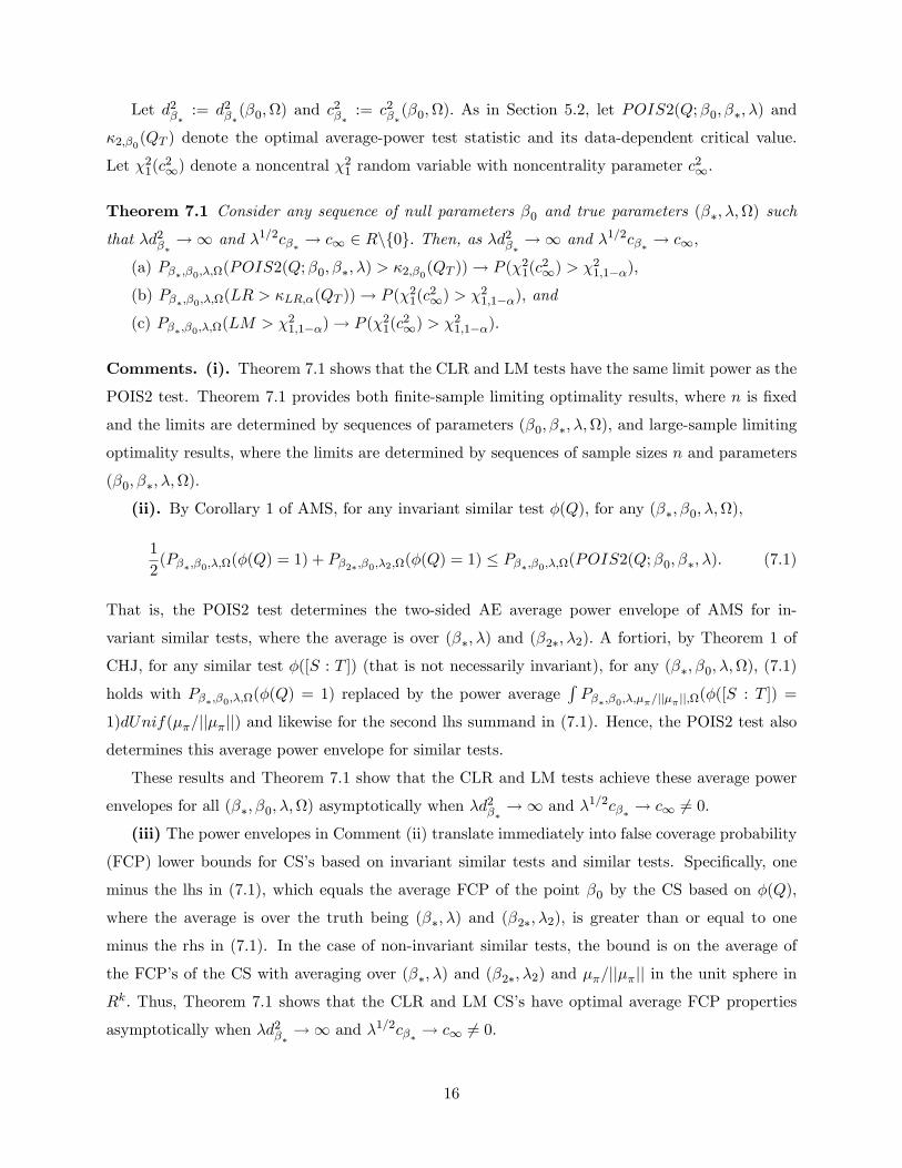
Let d2 := d2(0;) and c2:= c2(0;): As in Section 5.2, let POIS2(Q;0; ; ) and

2;0(QT ) denote the optimal average-power test statistic and its data-dependent critical value.

Let 21(c21) denote a noncentral

21 random variable with noncentrality parameter c21:

Theorem 7.1 Consider any sequence of null parameters 0 and true parameters (; ;) such

that d2 !1 and 1=2c ! c1 2 Rnf0g: Then, as d2 !1 and 1=2c ! c1;

(a) P;0;;(POIS2(Q;0; ; ) > 2;0(QT ))! P (21(c21) > 21;1);

(b) P;0;;(LR > LR;(QT ))! P (21(c21) > 21;1); and

(c) P;0;;(LM > 21;1)! P (21(c21) > 21;1):

Comments. (i). Theorem 7.1 shows that the CLR and LM tests have the same limit power as the

POIS2 test. Theorem 7.1 provides both nite-sample limiting optimality results, where n is xed

and the limits are determined by sequences of parameters (0; ; ;); and large-sample limiting

optimality results, where the limits are determined by sequences of sample sizes n and parameters

(0; ; ;):

(ii). By Corollary 1 of AMS, for any invariant similar test (Q); for any (; 0; ;);

1

2(P;0;;((Q) = 1) + P2;0;2;((Q) = 1) P;0;;(POIS2(Q;0; ; ): (7.1)

That is, the POIS2 test determines the two-sided AE average power envelope of AMS for in-

variant similar tests, where the average is over (; ) and (2; 2): A fortiori, by Theorem 1 of

CHJ, for any similar test ([S : T ]) (that is not necessarily invariant), for any (; 0; ;); (7.1)

holds with P;0;;((Q) = 1) replaced by the power averageRP;0;;=jj jj;(([S : T ]) =

1)dUnif(=jjjj) and likewise for the second lhs summand in (7.1). Hence, the POIS2 test alsodetermines this average power envelope for similar tests.

These results and Theorem 7.1 show that the CLR and LM tests achieve these average power

envelopes for all (; 0; ;) asymptotically when d2!1 and 1=2c ! c1 6= 0:

(iii) The power envelopes in Comment (ii) translate immediately into false coverage probability

(FCP) lower bounds for CSs based on invariant similar tests and similar tests. Specically, one

minus the lhs in (7.1), which equals the average FCP of the point 0 by the CS based on (Q);

where the average is over the truth being (; ) and (2; 2); is greater than or equal to one

minus the rhs in (7.1). In the case of non-invariant similar tests, the bound is on the average of

the FCPs of the CS with averaging over (; ) and (2; 2) and =jjjj in the unit sphere inRk: Thus, Theorem 7.1 shows that the CLR and LM CSs have optimal average FCP properties

asymptotically when d2 !1 and 1=2c ! c1 6= 0:

16

(iv). Theorem 7.1 does not apply when the IVs are completely irrelevant, i.e., = 0; because

= 0 implies that c1 = 0: However, Theorem 7.1 does cover some cases where the IVs can be

arbitrarily weak, see Theorem 7.2 below.

Next, we provide conditions under which d2 !1 and 1=2c ! c1 2 Rnf0g; as is assumedin Theorem 7.1. First, if 0 and are xed, is nonsingular, and (; ) satisfy !1 and

1=2( 0)! L 2 R as !1; (7.2)

then d2 ! 1 and 1=2c ! c1 2 Rnf0g with c1 = L(b00b0)1=2: Here L indexes the local

alternatives against which the tests have nontrivial power. This result covers the usual strong IV

case in which is xed, Z 0Z depends on n; and = 0Z 0Z !1 as n!1:The scenario in (7.2) also covers cases where = n ! 0 as n!1; but su¢ ciently slowly that

= 0nZ0Zn ! 1 as n ! 1; which covers semi-strongidentication. As far as we are aware,

this is the only optimality property in the literature for tests under semi-strong identication. The

scenario in (7.2) also covers nite-sample, i.e., xed n; cases in which Z 0Z is xed, diverges, i.e.,

jjjj ! 1; and min(Z 0Z) > 0: In these cases, = 0Z 0Z !1 as jjjj ! 1:The most novel cases in which Theorem 7.1 applies are when uv ! 1 or ! 1: The next

result shows that d2 !1 and 1=2c ! c1 2 Rnf0g when uv ! 1 or ! 1 and the otherparameters are xed at (almost) any values. It also shows that this holds when (uv; 0)! (1;1)or (1;1) or (; 0) ! (1;1) or (1;1) and the other parameters are xed at (almost)any values.

Theorem 7.2 (a) Suppose the parameters 0; ; u > 0; v > 0; and > 0 are xed, uv 2(1; 1); and uv ! 1: Then, (i) limuv!1

1=2c = 1=2( 0)=ju ( 0)vj and (ii)limuv!1 d

2=1 provided 0 6= u=v:

(b) Suppose the parameters 0; ; !1 > 0; !2 > 0; and > 0 are xed, 2 (1; 1); and ! 1: Then, (i) lim!1

1=2c = 1=2( 0)=j!1 !20j provided 0 6= !1=!2 and (ii)lim!1 d

2=1 provided 0 6= !1=!2 and 6= !1=!2:

(c) Suppose the parameters are as in part (a) except (uv; 0)! (1;1) or (1;1): Then, (i)lim(uv ;0)!(1;1)

1=2c = lim(uv ;0)!(1;1) 1=2c =

1=2=v and (ii) lim(uv ;0)!(1;1) d2

= lim(uv ;0)!(1;1) d2=1:

(d) Suppose the parameters are as in part (b) except (; 0)! (1;1) or (1;1): Then, (i)lim(;0)!(1;1)

1=2c = lim(;0)!(1;1) 1=2c = 1=2=!2 and (ii) lim(;0)!(1;1) d

2

=1 provided 6= !1=!2 and lim(;0)!(1;1) d2=1 provided 6= !1=!2:

17

Comments. (i). Combining Theorems 7.1 and 7.2 provides analytic nite-sample limiting opti-

mality results for the CLR and LM tests and CSs as uv ! 1 or ! 1 with 0 xed or jointlywith 0 ! 1 for (almost) any xed values of the other parameters. These results apply for any

strength of the IVs except = 0: These results are much stronger than typical weighted average

power (WAP) results because they hold for (almost) any xed values of the parameters 0; ; 1;

v; and > 0 when uv ! 1 and (almost) any xed values of the parameters 0; ; !1; !2; and > 0 when ! 1:

(ii). The cases uv ! 1 and ! 1 are closely related because (12)1=2!1 = (12uv)1=2uby (15.10) in the SM. Thus, uv ! 1 implies jj ! 1 and/or !1 ! 0: And, ! 1 impliesjuvj ! 1 and/or u ! 0:

8 General Power/False-Coverage-Probability Comparisons

By Theorem 4.1, the results in Table I equal power di¤erences (PDs) between the POIS2 and

CLR tests as the null value 0 ! 1 for xed true value = 0: Here, we consider PDs between

the POIS2 and CLR tests for nite 0 values, rather than PDs as 0 ! 1: Specically, TableII reports maximum and average PDs over 0 2 R and > 0 for a xed true value = 0 for a

range of values of (uv; k): As above, the choice of = 0 (and !21 = !22 = 1) is wlog. These PDs

are equivalent to false coverage probability di¤erences (FCPDs) between the CLR and POIS2 CSs

for a xed true value at incorrect values 0: They are necessarily nonnegative.

The values considered are 1; 3; 5; 7; 10; 15; 20; as well as 22; 25 when k = 20 and 40; and :7; :8; :9

when k = 2 and 5 and uv = :9: The positive and negative 0 values considered are those with

j0j 2 f:25; :5; :::; 3:75; 4; 5; 7:5; 10; 50; 100; 1000; 10000g:The number of simulation repetitions employed is 5; 000: The critical values are determined

using 100; 000 simulation repetitions. For example, the simulation standard deviations for the PDs

for (uv; k) = (0; 20) and any xed (0; ) value range from [:0013; :0040] across di¤erent (0; )

values, which compares to simulated averages of the PDs over (0; ) values that are of the :014

order of magnitude.

Tables II(a) and II(b) contain the same numbers, but are reported di¤erently to make the

patterns in the table more clear. Table II(a) shows variation across k for xed uv; whereas Table

II(b) shows variation across uv for xed k: The third and fourth columns in each table report the

values of and 0 at which the maximum PD is obtained. The fth column in each table reports

uv;0; which is the correlation between the structural-equation and reduced-form errors when 0

is the true value (based on the assumption that the consistently-estimable reduced-form variance

18

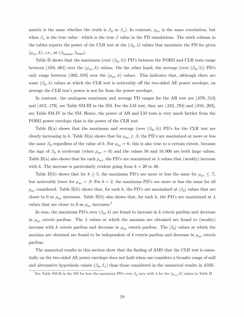
matrix is the same whether the truth is 0 or ): In contrast, uv is the same correlation, but

when is the true value which is the true value in the PD simulations. The sixth column in

the tables reports the power of the CLR test at the (0; ) values that maximize the PD for given

(uv; k); i.e., at (0;max; max):

Table II shows that the maximum (over (0; )) PDs between the POIS2 and CLR tests range

between [:016; :061] over the (uv; k) values. On the other hand, the average (over (0; )) PDs

only range between [:002; :016] over the (uv; k) values. This indicates that, although there are

some (0; ) values at which the CLR test is noticeably o¤ the two-sided AE power envelope, on

average the CLR tests power is not far from the power envelope.

In contrast, the analogous maximum and average PD ranges for the AR test are [:079; :513]

and [:012; :179]; see Table SM-III in the SM. For the LM test, they are [:242; :784] and [:010; :203];

see Table SM-IV in the SM. Hence, the power of AR and LM tests is very much farther from the

POIS2 power envelope than is the power of the CLR test.

Table II(a) shows that the maximum and average (over (0; )) PDs for the CLR test are

clearly increasing in k: Table II(a) shows that for uv :3; the PDs are maximized at more or less

the same 0 regardless of the value of k: For uv = 0; this is also true to a certain extent, because

the sign of 0 is irrelevant (when uv = 0) and the values 50 and 10; 000 are both large values.

Table II(a) also shows that for each uv; the PDs are maximized at values that (weakly) increase

with k: The increase is particularly evident going from k = 20 to 40:

Table II(b) shows that for k 5; the maximum PDs are more or less the same for uv :7;

but noticeably lower for uv = :9: For k = 2; the maximum PDs are more or less the same for all

uv considered. Table II(b) shows that, for each k; the PDs are maximized at j0j values that arecloser to 0 as uv increases. Table II(b) also shows that, for each k; the PDs are maximized at

values that are closer to 0 as uv increases.7

In sum, the maximum PDs over (0; ) are found to increase in k ceteris paribus and decrease

in uv ceteris paribus. The values at which the maxima are obtained are found to (weakly)

increase with k ceteris paribus and decrease in uv ceteris paribus. The j0j values at which themaxima are obtained are found to be independent of k ceteris paribus and decrease in uv ceteris

paribus.

The numerical results in this section show that the nding of AMS that the CLR test is essen-

tially on the two-sided AE power envelope does not hold when one considers a broader range of null

and alternative hypothesis values (0; ) than those considered in the numerical results in AMS.

7See Table SM-II in the SM for how the maximum PDs over 0 vary with for the (uv; k) values in Table II.

19

9 Di¤erences between CLR Power and an Average Over

Power Envelope

In this section, we introduce a WAP2power envelope for similar tests with weight functions

over: (i) a nite grid of values, fj > 0 : j Jg; (ii) the same two-points (; j) and (2; 2j)as in AMS for each j for j J; and (iii) the same uniform weight function over =jjjj as inCHJ. In particular, we use the uniform weight function over the 36 values of in f2:5; 5:0; :::; 90:0g:

The WAP2 envelope is a function of (0; ): The WAP2(Q; 0; ) test statistic that generates

this envelope is of the formPJj=1( (Q;0; j ; j)+ (Q;0; 2j ; 2j))=

PJj=1 2 2(QT ;0; ; j);

where the functions (Q;0; ; ) and 2(QT ;0; ; ) are as in AMS (and as in (11.5) in the SM).

The WAP2(Q; 0; ) conditional critical value 2;0;J(qT ) is dened to satisfy PQ1jQT (WAP2(Q;

0; ) > 2;0;J(qT )jqT ) = for all qT 0; where PQ1jQT (jqT ) denotes probability under thedensity fQ1jQT (jqT ); which is specied in (11.3) in the SM.

To be consistent with Tables I and II, we report PDs between the WAP2(Q; 0; ) and CLR

tests for = 0 and a range of 0 values. These PDs are equivalent to the FCPDs between

the CLR and WAP2 CSs for xed true and varying incorrect 0 values. The di¤erences are

necessarily nonnegative.

We consider uv 2 f0; :3; :5; :7; :9; :95; :99g; k = 2; 5; 10; 20; 40; the same 0 values as in Table II,and !21 = !22 = 1: Since = 0; = uv: Section 21 shows that taking = 0 and !

21 = !22 = 1 is

wlog provided the support of the weight function for is scaled by !22 when !2 6= 1: The numberof simulation repetitions employed is 1; 000 for each j value. With power averaged over the 36

j values and independence of the simulation draws across j ; this yields simulation SDs that

are comparable to using 36; 000 simulation repetitions. The critical values are determined using

100; 000 simulation repetitions for k = 5 and 10; 000 for other values of k:

For brevity, Table III reports results only for k = 5 for a subset of the 0 values considered.

Results for all values of k and 0 considered are given in Table SM-V in the SM. Table IV reports

summary results for all values of k: In particular, Table IV(a) provides the maxima over 0 of the

average over PDs for each (uv; k): Table IV(b) provides the average over 0 of the average over

PDs for each (uv; k):

Table III shows that the CLR test has power quite close to the WAP2 power envelope for k = 5:

The PDs for uv 2 f0; :3; :5; :7g; we have PD2 [:000; :005] and SD2 [:0003; :0007] across all 0values. For uv 2 f:9; :95; :99g; we have PD2 [:000; :001] and SD2 [:0000; :0003] across all 0 values.

Table IV shows that PDs between the WAP2 power envelope and the CLR power are increasing

in k and decreasing in juvj: For k = 2; the maximum PD over 0 and uv values is very small:

20

:004: In the worst case for CLR, which is when (k; uv) = (40; 0); the maximum PD over 0 values

is substantially larger: :024: The average (over 0 values) PD in this case is :013; which is not very

large. For k = 40 and uv :9; the maximum PD (over 0 and uv values) is very small: :004: This

is consistent with the theoretical optimality properties of the CLR test as uv ! 1 described inSection 7. For k = 40 and uv :9; the average PD (over 0 values and the ve uv values) is very

small: :000: The second worst case for CLR in Table V is when (k; uv) = (20; 0): In this case, the

maximum PD over 0 values is :013; which is noticeably lower than :024 for (k; uv) = (40; 0):

In conclusion, the results in Tables III and IV show that the CLR test is very close to the WAP2

power envelope for most (k; uv; 0) values, but can deviate from it by as much as :024 for some 0

values when (k; uv) = (40; 0):

21

References

Anderson, T. W. (1946): The Non-central Wishart Distribution and Certain Problems of Multi-

variate Statistics,Annals of Mathematical Statistics, 17, 409-431.

Anderson, T. W. and H. Rubin (1949): Estimation of the Parameters of a Single Equation in a

Complete System of Stochastic Equations,Annals of Mathematical Statistics, 20, 4663.

Andrews, D. W. K. (1998): Hypothesis Testing with a Restricted Parameter Space,Journal of

Econometrics, 84, 155199.

Andrews, D. W. K., and P. Guggenberger (2015): Identication- and Singularity-Robust Infer-

ence for Moment Condition Models,Cowles Foundation Discussion Paper No. 1978, Yale

University.

(2016): Asymptotic Size of Kleibergens LM and Conditional LR Tests for Moment Con-

dition Models,Econometric Theory, 32, forthcoming. Also available as Cowles Foundation

Discussion Paper No. 1977, Yale University.

Andrews, D. W. K., M. J. Moreira, and J. H. Stock (2004): Optimal Invariant Similar Tests for

Instrumental Variables Regression with Weak Instruments,Cowles Foundation Discussion

Paper No. 1476, Yale University.

(2006): Optimal Two-sided Invariant Similar Tests for Instrumental Variables Regres-

sion,Econometrica, 74, 715752.

Andrews, D. W. K. and W. Ploberger (1994): Optimal Tests When a Nuisance Parameter Is

Present Only Under the Alternative,Econometrica, 63, 13831414.

Chamberlain, G. (2007): Decision Theory Applied to an Instrumental Variables Model,Econo-

metrica, 75, 609652.

Chernozhukov, V., C. Hansen, and M. Jansson (2009): Admissible Invariant Similar Tests for

Instrumental Variables Regression,Econometric Theory, 25, 806818.

Dufour, J.-M. (1997): Some Impossibility Theorems in Econometrics with Applications to Struc-

tural and Dynamic Models,Econometrica, 65, 13651387.

Elliott, G., U. K. Müller, and M. W. Watson (2015): Nearly Optimal Tests When a Nuisance

Parameter Is Present Under the Null Hypothesis,Econometrica, 83, 771811.

22

Hillier, G. H. (1984): Hypothesis Testing in a Structural Equation: Part I, Reduced Form Equiv-

alence and Invariant Test Procedures,unpublished manuscript, Dept. of Econometrics and

Operations Research, Monash University.

(2009): Exact Properties of the Conditional Likelihood Ratio Test in an IV Regression

Model,Econometric Theory, 25, 915957.

Kleibergen, F. (2002): Pivotal Statistics for Testing Structural Parameters in Instrumental Vari-

ables Regression,Econometrica, 70, 1781-1803.

Mikusheva, A. (2010): Robust Condence Sets in the Presence of Weak Instruments,Journal

of Econometrics, 157, 236247.

Mills, B., M. J. Moreira, and L. P. Vilela (2014): Tests Based on t-Statistics for IV Regression

with Weak Instruments,Journal of Econometrics, 182, 351363.

Moreira, M. J. (2003): A Conditional Likelihood Ratio Test for Structural Models,Economet-

rica, 71, 1027-1048.

(2009): Tests with Correct Size When Instruments Can Be Arbitrarily Weak, Journal of

Econometrics, 152, 131140.

Moreira, H. and M. J. Moreira (2013): Contributions to the Theory of Optimal Tests,unpub-

lished manuscript, FGV/EPGE, Brasil.

van der Vaart, A. W. (1998): Asymptotic Statistics. Cambridge, UK: Cambridge University Press.

van der Vaart, A. W. and J. A. Wellner (1996): Weak Convergence and Empirical Processes. New

York: Springer.

Wald, A. (1943): Tests of Statistical Hypotheses Concerning Several Parameters When the Num-

ber of Observations Is Large,Transactions of the American Mathematical Society, 54, 426

482.

23

TABLE I. Differences in Probabilities of Infinite-Length CI’s for the CLR and POIS2∞ CI’s, and Probabilities ofInfinite-Length POIS2∞ CI’s as Functions of k, λ and ρuv

k λCLR–POIS2∞ POIS2∞

ρuv = 0 .3 .5 .7 .9 ρuv = 0 .7 .92 1 .002 .004 .003 .002 .002 .870 .863 .8502 3 .007 .003 .002 .001 .001 .680 .656 .6132 5 .012 .008 .003 .002 .001 .497 .455 .4102 7 .016 .005 .001 .001 -.000 .344 .298 .2622 10 .013 .006 .002 .001 .000 .184 .142 .1222 15 .008 .004 .002 .001 .001 .056 .035 .0292 20 .003 .001 .001 .000 -.000 .014 .008 .0075 1 .003 .003 .002 .002 .002 .900 .898 .8825 3 .010 .010 .006 .002 .004 .778 .751 .6715 5 .017 .012 .004 .003 -.001 .639 .576 .4665 7 .026 .012 .003 .001 -.002 .502 .407 .3045 10 .031 .016 .005 .004 .002 .323 .221 .1445 12 .029 .011 .003 .000 -.001 .231 .140 .0865 15 .023 .013 .005 .003 .001 .134 .062 .0365 20 .013 .007 .003 .001 .000 .048 .016 .0085 25 .006 .002 .001 .000 .000 .016 .004 .00110 1 .001 .002 .002 .001 .000 .919 .916 .90410 5 .018 .015 .008 .005 .004 .731 .667 .52610 10 .032 .014 .003 .005 .001 .459 .320 .17610 15 .037 .020 .009 .004 .000 .239 .111 .04610 17 .035 .017 .008 .003 .000 .176 .069 .02510 20 .027 .014 .006 .002 .000 .110 .032 .01010 25 .017 .008 .003 .001 .000 .045 .008 .00210 30 .009 .004 .002 .000 -.000 .017 .002 .00020 1 .001 .003 .002 .002 .000 .929 .926 .91920 5 .014 .011 .006 .003 .006 .809 .766 .62020 10 .035 .022 .011 .010 .001 .603 .463 .24620 15 .046 .025 .011 .008 .001 .390 .215 .07320 20 .044 .021 .011 .005 .000 .226 .080 .01820 30 .033 .012 .005 .001 .000 .056 .007 .00120 40 .007 .003 .001 .000 .000 .010 .001 .00040 1 .002 .001 .001 .001 .000 .937 .937 .93440 5 .011 .008 .005 .001 .009 .859 .838 .71740 10 .028 .020 .009 .009 .002 .721 .614 .35440 15 .043 .022 .011 .009 .001 .555 .372 .12940 20 .049 .029 .013 .009 .001 .394 .186 .03840 30 .043 .021 .011 .004 .000 .155 .028 .00240 40 .022 .012 .005 .001 .000 .046 .003 .00040 60 .002 .001 .000 .000 .000 .003 .000 .000

TABLE II. Maximum and Average Power Differences over λ and β0 Values between POIS2 and CLR Tests for Fixed Alternative β∗ = 0

(a) Across k patterns for fixed ρuv

POIS2–CLRρuv k λmax β0,max ρuv,0 POIS2 max average.0 2 7 −10000.00 1.00 .66 .021 .006.0 5 10 −50.00 1.00 .68 .030 .009.0 10 15 −50.00 1.00 .76 .038 .012.0 20 15 10.00 −1.00 .60 .042 .014.0 40 22 −50.00 1.00 .66 .059 .016.3 2 10 3.75 −0.96 .86 .019 .005.3 5 10 3.50 −0.96 .73 .034 .008.3 10 10 3.00 −0.94 .59 .032 .009.3 20 15 3.50 −0.96 .66 .045 .012.3 40 22 4.00 −0.97 .72 .061 .014.5 2 5 2.00 −0.87 .64 .016 .004.5 5 10 2.25 −0.90 .82 .029 .005.5 10 10 2.00 −0.87 .70 .037 .007.5 20 10 1.75 −0.82 .53 .046 .009.5 40 15 1.75 −0.82 .59 .050 .012.7 2 5 1.50 −0.75 .81 .016 .002.7 5 5 1.50 −0.75 .67 .033 .003.7 10 7 1.50 −0.75 .71 .036 .005.7 20 7 1.25 −0.61 .54 .042 .006.7 40 15 1.50 −0.75 .84 .050 .008.9 2 0.9 1.25 −0.63 .46 .017 .002.9 5 0.9 1.00 −0.22 .33 .017 .002.9 10 3 1.25 −0.63 .77 .027 .003.9 20 3 1.00 −0.22 .61 .032 .003.9 40 5 1.25 −0.63 .75 .040 .004

(b) Across ρuv patterns for fixed k

POIS2–CLRk ρuv λmax β0,max ρuv,0 POIS2 max average2 .0 7 −10000.00 1.00 .66 .021 .0062 .3 10 3.75 −0.96 .86 .019 .0052 .5 5 2.00 −0.87 .64 .016 .0042 .7 5 1.50 −0.75 .81 .016 .0022 .9 0.9 1.25 −0.63 .46 .017 .0025 .0 10 −50.00 1.00 .68 .030 .0095 .3 10 3.50 −0.96 .73 .034 .0085 .5 10 2.25 −0.90 .82 .029 .0055 .7 5 1.50 −0.75 .67 .033 .0035 .9 0.9 1.00 −0.22 .33 .017 .002

10 .0 15 −50.00 1.00 .76 .038 .01210 .3 10 3.00 −0.94 .59 .032 .00910 .5 10 2.00 −0.87 .70 .037 .00710 .7 7 1.50 −0.75 .71 .036 .00510 .9 3 1.25 −0.63 .77 .027 .00320 .0 15 10.00 −1.00 .60 .042 .01420 .3 15 3.50 −0.96 .66 .045 .01220 .5 10 1.75 −0.82 .53 .046 .00920 .7 7 1.25 −0.61 .54 .042 .00620 .9 3 1.00 −0.22 .61 .032 .00340 .0 22 −50.00 1.00 .66 .059 .01640 .3 22 4.00 −0.97 .72 .061 .01440 .5 15 1.75 −0.82 .59 .050 .01240 .7 15 1.50 −0.75 .84 .050 .00840 .9 5 1.25 −0.63 .75 .040 .004

2

TABLE III. Average (over λ) Power Differences for λ ∈ 2.5, 5.0, ..., 90.0 between the WAP2 and CLR Tests fork = 5

β0ρuv,0 WAP2–CLR

ρuv = 0 .9 ρuv = 0 .3 .5 .7 .9 .95 .99−10000.00 1.00 1.00 .005 .002 .001 .001 .000 -.000 .000−100.00 1.00 1.00 .005 .002 .001 .001 .000 -.001 -.000−10.00 1.00 1.00 .005 .002 .001 .000 .000 -.000 -.000−4.00 .97 1.00 .003 .001 .000 -.000 .000 .000 -.000−3.00 .95 .99 .003 .001 .000 .000 -.000 .001 .000−2.00 .89 .99 .002 .001 .000 .001 -.000 -.001 -.000−1.50 .83 .98 .001 .001 .001 .000 .000 -.001 -.000−1.00 .71 .97 .001 .000 -.000 -.000 -.000 .000 -.000−0.75 .60 .97 .000 -.000 .001 -.000 -.000 .000 .000−0.50 .45 .95 -.000 -.000 -.001 -.001 -.000 -.001 -.000−0.25 .24 .94 -.001 -.001 -.001 -.000 -.000 .001 -.001

0.25 −.24 .83 -.000 -.001 -.001 -.000 -.001 .000 .0000.50 −.45 .68 .001 .000 .000 .000 .000 -.001 .0000.75 −.60 .33 .000 .001 .001 .001 .000 .000 .0001.00 −.71 −.22 .002 .001 .001 .001 .000 .000 .0001.50 −.83 −.81 .001 .002 .003 .003 .001 -.000 .0002.00 −.89 −.93 .002 .003 .004 .002 .000 -.001 -.0003.00 −.95 −.98 .003 .005 .003 .001 .000 .000 .0004.00 −.97 −.99 .004 .005 .002 .001 .000 .001 .000

10.00 −1.00 −1.00 .005 .003 .001 .001 .000 .000 .000100.00 −1.00 −1.00 .005 .003 .001 .000 .000 -.001 .000

10000.00 −1.00 −1.00 .005 .002 .001 .001 .000 -.000 .000

TABLE IV. Average (over λ) Power Differences between the WAP2 and CLR Tests

k(a) Maxima over β0 (b) Averages over β0

ρuv = 0 .3 .5 .7 .9 .95 .99 ρuv = 0 .3 .5 .7 .9 .95 .992 .004 .003 .002 .002 .001 .001 .001 .002 .002 .001 .001 .000 .000 .0005 .005 .005 .004 .003 .001 .001 .000 .003 .002 .001 .001 .000 .000 .00010 .011 .010 .008 .005 .004 .003 .003 .007 .006 .004 .002 .001 .001 .00120 .013 .012 .010 .007 .002 .001 .002 .008 .007 .005 .002 .000 .000 .00040 .024 .021 .017 .011 .004 .001 .000 .013 .011 .007 .004 .000 .000 .000

Supplemental Material to A NOTE ON OPTIMAL INFERENCE IN THE LINEAR IV MODEL

By

Donald W. K. Andrews, Vadim Marmer, and Zhengfei Yu

January 2017

COWLES FOUNDATION DISCUSSION PAPER NO. 2073

COWLES FOUNDATION FOR RESEARCH IN ECONOMICS YALE UNIVERSITY

Box 208281 New Haven, Connecticut 06520-8281

http://cowles.yale.edu/

Supplemental Material

for

A Note on Optimal Inferencein the Linear IV Model

Donald W. K. Andrews

Cowles Foundation for Research in Economics

Yale University

Vadim Marmer

Vancouver School of Economics

University of British Columbia

Zhengfei Yu

Faculty of Humanities and Social Sciences

University of Tsukuba

First Version: October 23, 2015

Revised: January 30, 2017

Contents

10 Outline 2

11 Denitions 3

11.1 Densities of Q when = and when 0! 1 . . . . . . . . . . . . . . . . . . . . 3

11.2 POIS2 Test . . . . . . . . . . . . . . . . . . . . . . . . . . . . . . . . . . . . . . . . . 4

11.3 Structural and Reduced-Form Variance Matrices . . . . . . . . . . . . . . . . . . . . 4

12 One-Sided Power Bound as 0! 1 5

12.1 Point Optimal Invariant Similar Tests for Fixed 0 and . . . . . . . . . . . . . . 6

12.2 One-Sided Power Bound When 0! 1 . . . . . . . . . . . . . . . . . . . . . . . . 6

13 Equations (4.1) and (4.2) of AMS 8

14 Proof of Lemma 5.1 10

15 Proof of Theorem 4.1 12

16 Proofs of Theorems 5.2, Corollary 5.3, and Theorem 5.4 17

17 Proof of Theorem 7.1 25

18 Proofs of Theorem 12.1 and Lemmas 13.1 and 13.2 36

19 Power Against Distant Alternatives Compared to Distant Null Hypotheses 39

19.1 Scenario 1 Compared to Scenario 2 . . . . . . . . . . . . . . . . . . . . . . . . . . . . 39

19.2 Structural Error Variance Matrices under Distant Alternatives and Distant

Null Hypotheses . . . . . . . . . . . . . . . . . . . . . . . . . . . . . . . . . . . . . . 40

20 Transformation of the 0 Versus Testing Problem to a

0 Versus Testing Problem 41

21 Transformation of the 0 Versus Testing Problem to a

0 Versus 0 Testing Problem 45

22 Additional Numerical Results 46

1

10 Outline

References to sections, theorems, and lemmas with section numbers less than 10 refer to

sections and results in the main paper.

Section 11 of this Supplemental Material (SM) provides expressions for the densities

fQ(q;; 0; ;); fQ1jQT (q1jqT ); and fQ(q; uv; v); expressions for the POIS2 test statistic andcritical value of AMS, and expressions for the one-to-one transformations between the reduced-

form and structural variance matrices. Section 12 provides one-sided power bounds for invariant

similar tests as 0 ! 1; where 0 denotes the null hypothesis value. Section 13 corrects (4.1)of AMS, which concerns the two-point weight function that denes AMSs two-sided AE power

envelope.

Section 14 proves Lemma 5.1. Section 15 proves Theorem 4.1 and its Comment (v). Section 16

proves Theorem 5.2 and its Comment (iv), Corollary 5.3 and its Comment (ii), and Theorem 5.4.

Section 17 proves Theorem 7.1. Section 18 proves Theorem 12.1 and Lemmas 13.1 and 13.2.

Section 19 contrasts the power properties of tests in the scenario where 0 is xed and takes

on large (absolute) values, with the scenario where is xed and 0 takes on large (absolute)

values.

Section 20 shows how the model is transformed to go from a testing problem of H0 : = 0

versus H1 : = for 2 Rk and xed to a testing problem of H0 : = 0 versus H1 : =

for some 2 Rk and some xed with diagonal elements equal to one. This links the model

considered here to the model used in the Andrews, Moreira, and Stock (2006) (AMS) numerical

work.

Section 21 shows how the model is transformed to go from a testing problem of H0 : = 0

versus H1 : = for 2 Rk and xed to a testing problem of H0 : = 0 versus H1 : = 0 for

some 2 Rk and some xed with diagonal elements equal to one. These transformation resultsimply that there is no loss in generality in the numerical results of the paper to taking !21 = !22 = 1;

= 0; and uv 2 [0; 1] (rather than uv 2 [1; 1]):Section 22 provides numerical results that supplement the results given in Tables I-IV in the

main paper.

2

11 Denitions

11.1 Densities of Q when = and when 0! 1

In this subsection, we provide expressions for (i) the density fQ(q;; 0; ;) of Q when the

true value of is ; and the null value 0 is nite, (ii) the conditional density fQ1jQT (q1jqT ) of Q1given QT = qT ; and (iii) the limit of fQ(q;; 0; ;) as 0 ! 1:

Let

(q) = (q;0;) := c2qS + 2cdqST + d2qT ; (11.1)

where c = c(0;) and d = d(0;): As in Section 5, fQ(q;; 0; ;) denotes the density

of Q := [S : T ]0[S : T ] when [S : T ] has the multivariate normal distribution in (2.3) with =

and = 0: This noncentral Wishart density is

fQ(q;; 0; ;) = K1 exp((c2 + d2)=2) det(q)(k3)=2 exp((qS + qT )=2)

((q))(k2)=4I(k2)=2(

q(q)); where

q =

24 qS qST

qST qT

35 ; q1 =0@ qS

qST

1A 2 R+ R; qT 2 R+; (11.2)

K11 = 2(k+2)=2pi1=2((k 1)=2); I() denotes the modied Bessel function of the rst kind of

order ; pi = 3:1415:::; and () is the gamma function. This holds by Lemma 3(a) of AMS with = :

By Lemma 3(c) of AMS, the conditional density of Q1 given QT = qT when [S : T ] is distributed

as in (2.3) with = 0 is

fQ1jQT (q1jqT ) := K1K12 exp(qS=2) det(q)(k3)=2q(k2)=2T ; (11.3)

which does not depend on 0; ; or :

By Lemma 5.1, the limit of fQ(q;; 0; ;) as 0 ! 1 is the density fQ(q; uv; v): As in

Section 5, fQ(q; uv; v) denotes the density of Q := [S : T ]0[S : T ] when [S : T ] has a multivariate

normal distribution with means matrix in (5.2), all variances equal to one, and all covariances equal

to zero. This is a noncentral Wishart density that has following form:

fQ(q; uv; v) = K1 exp(v(1 + r2uv)=2) det(q)(k3)=2 exp((qS + qT )=2)

(v(q; uv))(k2)=4I(k2)=2(pv(q; uv)); where

(q; uv) := qS + 2ruvqST + r2uvqT : (11.4)

3

This expression for the density holds by the proof of Lemma 3(a) of AMS with means matrix

(1=v; ruv=v) in place of the means matrix (c ; d):

11.2 POIS2 Test

Here we dene the POIS2(q1; qT ;0; ; ) test statistic of AMS, which is analyzed in Section

5, and its conditional critical value 2;0(qT ):

Given (; ); the parameters (2; 2) are dened in (5.3), which is the same as (4.2) of AMS.

By Cor. 1 of AMS, the optimal average-power test statistic against (; ) and (2; 2) is

POIS2(Q;0; ; ) := (Q;0; ; ) + (Q;0; 2; 2)

2 2(QT ;0; ; ); where

(Q;0; ; ) := exp((c2 + d2)=2)((Q))(k2)=4I(k2)=2(q(Q));

2(QT ;0; ; ) := exp(d2=2)(d2QT )(k2)=4I(k2)=2(qd2QT ); (11.5)

Q and QT are dened in (3.1), c = c(;) and d = d(;) are dened in (2.3), I() is denedin (11.2), (Q) is dened in (11.1) with Q and in place of q and ; and := 0: Note that

2(QT ;; ) = 2(QT ;2; 2) by (5.3).

Let 2;0(qT ) denote the conditional critical value of the POIS2(Q;0; ; ) test statistic. That

is, 2;0(qT ) is dened to satisfy

PQ1jQT (POIS2(Q;0; ; ) > 2;0(qT )jqT ) = (11.6)

for all qT 0; where PQ1jQT (jqT ) denotes probability under the density fQ1jQT (jqT ) dened in(11.3). The critical value function 2;0() depends on (0; ; ;) and k (and (2; 2) through(; )).

11.3 Structural and Reduced-Form Variance Matrices

Let ui; v1i; and v2i denote the ith elements of u; v1; and v2; respectively. We have

v1i := ui + v2i and =

24 !21 !12

!12 !22

35 ; (11.7)

where denotes the true value.

Given the true value and some structural error variance matrix ; the corresponding reduced-

4

form error variance matrix (;) is

(;) := V ar

0@0@ v1i

v2i

1A1A = V ar

0@0@ ui + v2i

v2i

1A1A=

24 1

0 1

3524 1 0

1

35 =24 2u + 2uv +

2v2 uv +

2v

uv + 2v 2v

35 ; where =

24 2u uv

uv 2v

35 : (11.8)

Given the true value and the reduced-form error variance matrix ; the structural variance

matrix (;) is

(;) := V ar

0@0@ ui

v2i

1A1A = V ar

0@0@ v1i v2iv2i

1A1A (11.9)

=

24 1 0 1

3524 1 0

1

35 =24 !21 2!12 + !222 !12 !22

!12 !22 !22

35 :Let 2u(;);

2v(;); and uv(;) denote the (1; 1); (2; 2); and (1; 2) elements of (;): Let

uv(;) denote the correlation implied by (;):

In the asymptotics as 0 ! 1; we x and and consider the testing problem as 0 ! 1:Rather than xing ; one can equivalently x the structural variance matrix when = ; say at

: Given and ; there is a unique reduced-form error variance matrix = (;) dened

using (11.8). Signicant simplications in certain formulae occur when they are expressed in terms

of ; rather than ; e.g., see Lemma 14.1(e) below.

For notational simplicity, we denote the (1; 1); (2; 2); and (1; 2) elements of by 2u; 2v; and

uv; respectively, without any subscripts. As dened in (4.5), uv := uv=(uv): Thus, uv is the

correlation between the structural and reduced-form errors ui and v2i when the true value of is

: Note that uv does not change when (;) is xed (or, equivalently, (;) = (;(;))

is xed) and 0 is changed. Also, note that 2v = !22 because both denote the variance of v2i under

= and = 0:

12 One-Sided Power Bound as 0! 1

In this section, we provide one-sided power bounds for invariant similar tests as 0 ! 1 for

xed : The approach is the same as in Andrews, Moreira, and Stock (2004) (AMS04) except that

5

we consider 0 ! 1: Also see Mills, Moreira, and Vilela (2014).

12.1 Point Optimal Invariant Similar Tests for Fixed 0 and

First, we consider the point null and alternative hypotheses:

H0 : = 0 and H1 : = ; (12.1)

where 2 Rk (or, equivalently, 0) under H0 and H1:Point optimal invariant similar (POIS) tests for any given null and alternative parameter values

0 and ; respectively, and any given are constructed in AMS04, Sec. 5. Surprisingly, the same

test is found to be optimal for all values of under H1; i.e., for all strengths of identication.

The optimal test is constructed by determining the level test that maximizes conditional power

given QT = qT among tests that are invariant and have null rejection probability conditional on

QT = qT ; for each qT 2 R:By AMS04 (Comment 2 to Cor. 2), the POIS test of H0 : = 0 versus H1 : = ; for any

2 Rk (or 0) under H1; rejects H0 for large values of

POIS(Q;0; ) := QS + 2d(0;)

c(0;)QST : (12.2)

The critical value for the POIS(Q;0; ) test is a conditional critical value given QT = qT ; which

we denote by 0(qT ): The critical value 0(qT ) is dened to satisfy

PQ1jQT (POIS(Q;0; ) > 0(qT )jqT ) = (12.3)

for all qT 0; where PQ1jQT (jqT ) denotes probability under the conditional density fQ1jQT (q1jqT )dened in (11.3). Although the density fQ1jQT (q1jqT ) does not depend on 0; 0(qT ) depends on0; as well as (;; k); because POIS(Q;0; ) does.

Note that, although the same POIS(Q;0; ) test is best for all strengths of identication,

i.e., for all = 0 > 0; the power of this test depends on :

12.2 One-Sided Power Bound When 0! 1

Now we consider the best one-sided invariant similar test as 0 ! 1 keeping (;) xed.

Lemma 14.1 below implies that

lim0!1

d(0;)

c(0;)=

uvv(1 2uv)1=2

= (1=v) =

uv(1 2uv)1=2

; (12.4)

6

where uv; dened in (4.5), is the correlation between the structural and reduced-form errors ui

and v2i under : Hence, the limit as 0 ! 1 of the POIS(Q;0; ) test statistic in (12.2) is

POIS(Q;1; uv) := lim0!1

QS + 2

d(0;)

c(0;)QST

= QS + 2

uv(1 2uv)1=2

QST : (12.5)

Notice that (i) this limit is the same for 0 ! +1 and 0 ! 1; (ii) the POIS(Q;1; uv) statisticdepends on (;) = (;(;)) only through uv := Corr(); and (iii) when uv = 0;

the POIS(Q;1; uv) statistic is the AR statistic (times k): Some intuition for result (iii) is thatEQST = 0 under the null and limj0j!1EQST = 0 under any xed alternative when uv = 0

(see the discussion in Section 5.2). In consequence, QST is not useful for distinguishing between

H0 and H1 when j0j ! 1 and uv = 0:

Let 1(qT ) denote the conditional critical value of the POIS(Q;1; uv) test statistic. That is,1(qT ) is dened to satisfy

PQ1jQT (POIS(Q;1; uv) > 1(qT )jqT ) = (12.6)

for all qT 0: The density fQ1jQT (jqT ) of PQ1jQT (jqT ) only depends on the number of IVs k; see(11.3). The critical value function 1() depends on uv and k:

Let 0(Q) denote a test of H0 : = 0 versus H1 : = based on Q that rejects H0 when

0(Q) = 1: In most cases, a test depends on 0 because the distribution of Q depends on 0; see

(2.3) and (3.1), and not because 0() depends on 0: For example, this is true of the AR, LM,and CLR tests in (3.3) and (3.4). However, we allow for dependence of 0() on 0 in the followingresult in order to cover all possible sequences of (non-randomized) tests of H0 : = 0:

Theorem 12.1 Let f0(Q) : 0 ! 1g be any sequence of invariant similar level tests ofH0 : = 0 versus H1 : = when Q has density fQ(q;; 0; ;) for some 0 and is xedand known. For xed true (; ;); the POIS(Q;1; uv) test satises

lim sup0!1

P;0;;(0(Q) = 1) Puv ;v(POIS(Q;1; uv) > 1(QT )):

Comments. (i). Theorem 12.1 shows that the POIS(Q;1; uv) test provides an asymptoticpower bound as 0 ! 1 for any invariant similar test for any xed (; ;): This power bound

is strictly less than one. The reason is that lim0!1 jc(0;)j 9 1: This is the same reasonthat the AR test does not have power that converges to one in this scenario, see Section 19. Hence,

the bound in Theorem 12.1 is informative.

(ii). The power bound in Theorem 12.1 only depends on (; ;) through uv; the magnitude

7

of endogeneity under ; and v; the concentration parameter:

(iii). As an alternative to the power bound given in Theorem 12.1, one might consider develop-

ing a formal limit of experiments result, e.g., along the lines of van der Vaart (1998, Ch. 9). This

approach does not appear to work for the sequence of experiments consisting of the two uncondi-

tional distributions of [S : T ] (or Q) for = 0; and indexed by 0 as 0 ! 1: The reasonis that the likelihood ratio of these two distributions is asymptotically degenerate as 0 ! 1(either 0 or 1 depending on which density is in the numerator) when the truth is taken to be

= 0: This occurs because the length of the mean vector of T diverges to innity as 0 ! 1(provided = 0 > 0) by (2.3) and Lemma 14.1(c) below. For the sequence of conditional

distributions of Q given QT = qT ; it should be possible to obtain a formal limit of experiments

result, but this would not very helpful because we are interested in the unconditional power of tests

and a conditional limit of experiments result would not deliver this.

(iv). The proof of Theorem 12.1 is given in Section 18 below.

13 Equations (4.1) and (4.2) of AMS

This section corrects (4.1) of AMS, which concerns the two-point weight function that denes

AMSs two-sided AE power envelope.

Equation (4.1) of AMS is:8 given (; ); the second point (2; 2) solves

1=22 c2 =

1=2c (6= 0) and 1=22 d2 = 1=2d : (13.1)

AMS states that provided 6= AR; the solutions to the two equations in (4.1) satisfy the two

equations in (4.2) of AMS, which is the same as (5.3) and which we repeat here for convenience:9

2 = 0 d0( 0)

d0 + 2r0( 0)and 2 =

(d0 + 2r0( 0))2

d20; where

r0 := e011a0 (a001a0)1=2 and e1 := (1; 0)0: (13.2)

Equation (4.2) is correct as stated, but (4.1) of AMS is not correct. More specically, it is not

complete. It should be: given (; ); the second point (2; 2) solves either (13.1) or

1=22 c2 = 1=2c (6= 0) and

1=22 d2 =

1=2d : (13.3)

8Note that (; ) and (2; 2) in this paper correspond to (; ) and (2;

2) in AMS.

9The formulae in (5.3) and (13.2) only hold for 6= AR; where AR := (!21 !120)=(!12 !220) provided!12 !220 6= 0 (which necessarily holds for j0j su¢ ciently large because !22 > 0):

8

For brevity, we write the either orconditions in (13.1) and (13.3) as

1=22 c2 =

1=2c (6= 0) and 1=22 d2 =

1=2d : (13.4)

The reason (4.1) of AMS needs to be augmented by (13.3) is that for some (; ); 0; and

; (4.1) has no real solutions (2; 2) and the expressions for (2; 2) in (4.2) of AMS do not

satisfy (4.1). Once (4.1) of AMS is augmented by (13.3), there exist real solutions (2; 2) to the

augmented conditions and they are given by the expressions in (4.2) of AMS, i.e., by (13.2). This

is established in the following lemma.

Lemma 13.1 The conditions in (13.4) hold i¤ the conditions in (4.2) of AMS hold, i.e., i¤ the

conditions in (13.2) holds.

With (4.1) of AMS replaced by (13.4), the results in Theorem 8(b) and (c) of AMS hold as

stated. That is, the two-point weight function that satises (13.4) leads to a two-sided weighted

average power (WAP) test that is asymptotically e¢ cient under strong IVs. And, all other two-

point weight functions lead to two-sided WAP tests that are not asymptotically e¢ cient under

strong IVs.

Lemma 13.2 Under the assumptions of Theorem 8 of AMS, i.e., Assumptions SIV-LA and 1-4 of

AMS, (a) if (2; 2) satises (13.4); then LR( bQ1;n; bQT;n; ; ) = e

12()2 cosh(LM

1=2n )+op(1);

where = 1=2c ; which is a strictly-increasing continuous function of LMn; and (b) if (2; 2)

does not satisfy (13.4), then LR( bQ1;n; bQT;n;; ) = 2(QST;n=Q1=2T;n) + op(1) for a continuous

function 2() that is not even.

Comments. (i). Lemma 13.2(a) is an extension of Theorem 8(b) of AMS; while Lemma 13.2(b)

is a correction to Theorem 8(c) of AMS.

(ii). The proofs of Lemma 13.1 and 13.2 are given in Section 18 below.

Having augmented (4.1) by (13.3), the two-point weight function of AMS does not have the

property that 2 is necessarily on the opposite side of 0 from : However, it does have the

properties that (i) for any (; ); (2; 2) is the only point that yields a two-point WAP test

that is asymptotic e¢ cient in a two-sided sense under strong IVs, (ii) the marginal distributions

of QS ; QT; and QST are the same under (; ) and (2; 2); and (iii) the joint distribution of

(QS ; QST ; QT ) under (; ) is the same as that of (QS ;QST ; QT ) under (2; 2):

9

14 Proof of Lemma 5.1

The proof of Lemma 5.1 and other proofs below use the following lemma.

The distributions of [S : T ] under (0;) and (;) depend on c(0;) and d(0;) for

= 0 and : The limits of these quantities as 0 ! 1 are given in the following lemma.10

Lemma 14.1 For xed and positive denite matrix ; we have

(a) lim0!1 c0(0;) = 0:

(b) lim0!1 c(0;) = 1=v:(c) lim0!1 d0(0;) =1:(d) d0(0;)=j0j =

!2(!21!

22!212)1=2

+ o(1) = 1u(12uv)1=2

+ o(1) as j0j ! 1:

(e) lim0!1 d(0;) = !22!12

!2(!21!22!212)1=2

= uvv(12uv)1=2

:

Comment. The limits in parts (d) and (e), expressed in terms of ; only depend on uv; u; and

v and their functional forms are of a relatively simple multiplicative form. The latter provides

additional simplications of certain quantities that appear below.

Proof of Lemma 14.1. Part (a) holds because c0(0;) = 0 for all 0: Part (b) holds by the

following calculations:

lim0!1

c(0;) = lim0!1

( 0) (b00b0)1=2

= lim0!1

( 0) (!21 2!120 + !2220)1=2

= 1=!2

= 1=v: (14.1)

Now, we establish part (e). Let b := (1;)0: We have

lim0!1

d(0;) = lim0!1

b0b0 (b00b0)1=2 det()1=2

= lim0!1

!21 !12 !120 + !220(!21 2!120 + !2220)1=2(!21!22 !212)1=2

= !22 !12!2(!21!

22 !212)1=2

: (14.2)

Next, we write the limit in (14.2) in terms of the elements of the structural error variance matrix

10Throughout, 0 ! 1 means 0 !1 or 0 ! 1:

10

: The term in the square root in the denominator of (14.2) satises

!21!22 !212 = (2u + 2uv + 2v2)2v (uv + 2v)2 = 2u

2v 2uv; (14.3)

where the rst equality uses !22 = 2v (since both denote the variance of v2i); !21 = 2u + 2uv +

2v2); and !12 = uv+

2v (which both hold by (11.8) with = and = ); and the second

equality holds by simple calculations. The limit in (14.2) in terms of the elements of is

!22 !12!2(!21!

22 !212)1=2

= 2v (uv + 2v)v(2u

2v 2uv)1=2

= uvv(1 2uv)1=2

; (14.4)

where the rst equality uses (14.3), !22 = 2v; and !12 = uv + 2v; and the second inequality

holds by dividing the numerator and denominator by uv: This establishes part (e).

For part (c), we have

lim0!1

d0(0;) = lim0!1

(b00b0)1=2 det()1=2

= lim0!1

(!21 2!120 + !2220)1=2

(!21!22 !212)1=2

= 1: (14.5)

Part (d) holds because, as j0j ! 1; we have

d0(0;)=j0j =(!21=

20 2!12=0 + !22)1=2

(!21!22 !212)1=2

=!2

(!21!22 !212)1=2

+ o(1)

=1

u(1 2uv)1=2+ o(1); (14.6)

where the last equality uses (14.3) and !2 = v:

Next, we prove Lemma 5.1, which states that for any xed (; ;); lim0!1 fQ(q;; 0; ;)

= fQ(q; uv; v):

Proof of Lemma 5.1. By Lemma 14.1(b) and (e) and (5.1), we have lim0!1 c = 1=v and

11

lim0!1 d = ruv=v: In consequence,

lim0!1

(c2 + d2) = (1=2v)(1 + r

2uv) = v(1 + r

2uv) and

lim0!1

(q) = lim0!1

(c2qS + 2cdqST + d2qT )

= (1=2v)(qS + 2ruvqST + r2uvqT ) = v(q; uv); (14.7)

using the denitions of v and (q; uv) in (5.1) and (11.4), respectively, where the rst equality in

the third line uses (1)(ruv) = ruv: Combining this with (11.2) and (11.4) proves the result of

the lemma.

15 Proof of Theorem 4.1

The proof of Theorem 4.1 uses the following lemma.11 Let

S1(Y ) := (Z 0Z)1=2Z 0Y e2 1v;

T1(Y ) := (Z 0Z)1=2Z 0Y 1e1 ((1 2uv)1=2u); and

Q1(Y ) :=

24 e02Y0PZY e2 12v e02Y

0PZY 1e1 (1

2uv)

1=2uv

e02Y0PZY

1e1 (12uv)

1=2uv

e011Y 0PZY

1e1 (1 2uv)2u

35 ; (15.1)where uv := Corr(ui; v2i); PZ := Z(Z 0Z)1Z 0; e1 := (1; 0)0; and e2 := (0; 1)0: Let QT;1(Y ) denote

the (2; 2) element of Q1(Y ): As dened in (5.1), ruv = uv=(1 2uv)1=2:

Lemma 15.1 For xed and positive denite matrix ; we have

(a) lim0!1 S0(Y ) = S1(Y );

(b) S1(Y ) N( 1v; Ik);

(c) lim0!1 T0(Y ) = T1(Y ) = (Z 0Z)1=2Z 0Y 1e1((12)1=2!1); where := Corr(v1i; v2i);

(d) T1(Y ) N ruvv; Ik

;

(e) S1(Y ) and T1(Y ) are independent,

(f) lim0!1Q0(Y ) = Q1(Y ); and

(g) Q1(Y ) has a noncentral Wishart distribution with means matrix ( 1v ;ruvv) 2 Rk2;

identity variance matrix, and density given in (11.4).

Comment. The convergence results in Lemma 15.1 hold for all realizations of Y:11The proof of Comment (v) to Theorem 4.1 is the same as that of Theorem 4.1(a) and (b) with [S0(Y ); T0(Y )]

and T0(Y ) in place of Q0(Y ) and QT;0(Y ); respectively.

12

Proof of Theorem 4.1. First, we prove part (a). We have

1(RLength(CS(Y )) =1)

= 1(T (Q0(Y )) cv(QT;0(Y )) 80 K(Y ) for some K(Y ) <1)

= lim0!1

1(T (Q0(Y )) cv(QT;0(Y ))); (15.2)

where the second equality holds provided the limit as 0 !1 on the rhs exists, the rst equality

holds by the denition of CS(Y ) in (4.1)-(4.3) and the denition of RLength(CS(Q)) = 1in (4.4), and the second equality holds because its rhs equals one (when the rhs limit exists) i¤

T (Q0(Y )) cv(QT;0(Y )) for 80 K(Y ) for some K(Y ) <1; which is the same as its lhs.Now, we use the dominated convergence theorem to show

lim0!1

E;;1(T (Q0(Y )) cv(QT;0(Y )))

= E;; lim0!1

1(T (Q0(Y )) cv(QT;0(Y ))): (15.3)

The dominated convergence theorem applies because (i) the indicator functions in (15.3) are domi-

nated by the constant function equal to one, which is integrable, and (ii) lim0!1 1(T (Q0(Y )) cv(QT;0(Y )) exists a.s.[P;;] and equals 1(T (Q1(Y )) cv(QT;1(Y )) a.s.[P;;]. The lat-

ter holds because the assumption that T (q) and cv(qT ) are continuous at positive denite (pd) qand positive qT ; respectively, coupled with the result of Lemma 15.1(f) (that Q0(Y ) ! Q1(Y )

as 0 ! 1 for all sample realizations of Y; where Q1(Y ) is dened in (15.1)), imply that (a)

lim0!1 T (Q0(Y )) = T (Q1(Y )) for all realizations of Y for which Q1(Y ) is pd, (b) lim0!1

cv(QT;0(Y )) = cv(QT;1(Y )) for all realizations of Y with QT;1(Y ) > 0; and hence (c) lim0!1

1(T (Q0(Y )) cv(QT0(Y )) = 1(T (Q1(Y )) cv(QT;1(Y )) for all realizations of Y for which

T (Q1(Y )) 6= cv(QT;1(Y )): We have P;;(T (Q1(Y )) = cv(QT;1(Y ))) = 0 by assumption, and

P;;(Q1(Y ) is pd & QT;1(Y ) > 0) = 1 (because Q1(Y ) has a noncentral Wishart distribution

by Lemma 15.1(g)). Thus, condition (ii) above holds and the DCT applies.

Next, we have

1 lim0!1

P;0;;((Q) = 1)

= lim0!1

E;;1(T (Q0(Y )) cv(QT;0(Y )))

= E;; lim0!1

1(T (Q0(Y )) cv(QT;0(Y )))

= P;;(RLength(CS(Y )) =1); (15.4)

13

where the rst equality holds because the distribution ofQ under P;0;;() equals the distributionof Q0(Y ) under P;;() and (Q) = 0 i¤ T (Q0) cv(QT ) by (4.2), the second equality holds

by (15.3), and the last equality holds by (15.2). Equation (15.4) establishes part (a).

The proof of part (b) is the same as that of part (a), but with LLength; 80 K(Y );0 ! 1; Q1(Y ); and QT;1(Y ) in place of RLength; 80 K(Y ); 0 ! 1; Q1(Y ); andQT;1(Y ); respectively.

The proof of part (c) uses the following: (i) Q1(Y ) and Q1(Y ) only di¤er in the sign of their

o¤-diagonal elements by (15.1), (ii) T (Q1(Y )) does not depend on the sign of the o¤-diagonalelement of Q1(Y ) by assumption, and hence, (iii) 1(T (Q1(Y )) cv(QT;1(Y )) = 1(T (Q1(Y )) cv(QT;1(Y )) for all sample realizations of Y: We have

1(RLength(CS(Y )) =1 & LLength(CS(Y )) =1)

= 1(T (Q0(Y )) cv(QT0(Y )) 80 K(Y ) & 80 K(Y ) for some K(Y ) <1)

= lim0!1

1(T (Q0(Y )) cv(QT;0(Y )) & T (Q0(Y )) cv(QT;0(Y )))

= 1(T (Q1(Y )) cv(QT;1(Y )) & T (Q1(Y )) cv(QT;1(Y )))

= 1(T (Q1(Y )) cv(QT;1(Y ))

= lim0!1

1(T (Q0(Y )) cv(QT;0(Y )) (15.5)

where the rst two equalities hold for the same reasons as the equalities in (15.2), the third equality

holds a.s.[P;;] by result (ii) that follows (15.3) and the same result with 0 and 1 in place of

0 and 1; respectively, the second last equality holds by condition (iii) immediately above (15.5),and the last equality holds by result (ii) that follows (15.3).

Now, we have

P;;(RLength(CS(Y )) =1 & LLength(CS(Y )) =1)

= E;; lim0!1

1(T (Q0(Y )) cv(QT;0(Y )))

= 1 lim0!1

P;0;;((Q) = 1); (15.6)

where the rst equality holds by (15.5) and the second equality holds by the rst four lines of

(15.4). This establishes the equality in part (c) when 0 ! 1: The equality in part (c) when0 ! 1 holds because (15.5) and (15.6) hold with 0 ! 1 replaced by 0 ! 1 since the

indicator function on the rhs of the second equality in (15.5) depends on 0 only through j0j:

14

Proof of Lemma 15.1. Part (a) holds because

lim0!1

S0(Y ) = lim0!1

(Z 0Z)1=2Z 0Y b0 (b00b0)1=2

= (Z 0Z)1=2Z 0Y lim0!1

0@ 1

0

1A =(!21 2!120 + !2220)1=2

= (Z 0Z)1=2Z 0Y e2(1=v); (15.7)

where e2 := (0; 1)0; the rst equality holds by (2.3), the second equality holds because b0 :=

(1;0)0; and the third equality holds using !2 = v:

Next, we prove part (b). The statistic S1(Y ) has a multivariate normal distribution because

it is a linear combination of multivariate normal random variables. The mean of S1(Y ) is

ES1(Y ) = (Z0Z)1=2Z 0Z[ : ]e2

1v

= (Z 0Z)1=2 1v

= 1v; (15.8)

where the rst equality holds using (2.2) with a = (; 1)0 and (15.1). The variance matrix of

S1(Y ) is

V ar(S1(Y )) = V ar((Z 0Z)1=2Z 0Y e2)=2v = V ar

nXi=1

(Z 0Z)1=2ZiY0i e2

!=2v

=nXi=1

V ar((Z 0Z)1=2ZiY0i e2)=

2v =

nXi=1

(Z 0Z)1=2ZiZi(Z0Z)1=2e02e2=

2v = Ik; (15.9)

where the third equality holds by independence across i and the last equality uses !22 = 2v: This

establishes part (b).

To prove part (c), we have

lim0!1

T0(Y ) = lim0!1

(Z 0Z)1=2Z 0Y 1a0 (a001a0)1=2

= (Z 0Z)1=2Z 0Y 1 lim0!1

0@ 0

1

1A =(!1120 + 2!120 + !

22)1=2

= (Z 0Z)1=2Z 0Y 1e1 (1=!11)1=2

= (Z 0Z)1=2Z 0Y 1e1 ((!21!22 !212)1=2=!2); (15.10)

where !11; !12; and !22 denote the (1; 1); (1; 2); and (2; 2) elements of 1; respectively, e1 := (1; 0)0;

the rst equality holds by (2.3), the second equality holds because a0 := (0; 1)0; and the fourth

15

equality holds by the formula for !11: In addition, we have

(!21!22 !212)1=2=!2 = (1 2)1=2!1 = (1 2uv)1=2u; (15.11)

where the rst equality uses := !12=(!1!2) and the second equality holds because !21!22!212 =

2u2v 2uv by (14.3) and !2 = v: Equations (15.10) and (15.11), combined with (15.1), establish

part (c).

Now, we prove part (d). Like S1(Y ); T1(Y ) has a multivariate normal distribution. The

mean of T1(Y ) is

ET1(Y ) = (Z 0Z)1=2Z 0Z[ : ]1e1 ((1 2uv)1=2u)

= (Z 0Z)1=2(!11 + !12) ((1 2uv)1=2u); (15.12)

where the equality holds using (2.2) with a = (; 1)0 and (15.1). In addition, we have

!11 + !12 =

!22 !12

!21!22 !212

=uv

2u2v 2uv

=uv

(1 2uv)uv; (15.13)

where the second equality uses !21!22 !212 = 2u

2v 2uv by (14.3) and !

22 !12 = uv by

(11.9) with = : Combining (15.12) and (15.13) gives

ET1(Y ) = uv

v(1 2uv)1=2=

ruvv

: (15.14)

The variance matrix of T1(Y ) is

V ar(T1(Y )) = V ar((Z 0Z)1=2Z 0Y 1e1) (1 2uv)2u

= V ar

nXi=1

(Z 0Z)1=2ZiY0i

1e1

! (1 2uv)2u =

nXi=1

V ar((Z 0Z)1=2ZiY0i

1e1) (1 2uv)2u

=nXi=1

(Z 0Z)1=2ZiZi(Z0Z)1=2e01

1e1 (1 2uv)2u = Ik!22

!21!22 !212

(1 2uv)2u

= Ik2v

2u2v 2uv

(1 2uv)2u = Ik;

where the rst equality holds by (15.1), the third equality holds by independence across i; and the

second last equality uses !21!22 !212 = 2u

2v 2uv by (14.3) and !22 = 2v:

16

Part (e) holds because

Cov(S1(Y ); T1(Y )) = nXi=1

Cov((Z 0Z)1=2ZiY0i e2; (Z

0Z)1=2ZiY0i

1e1) (1 2uv)1=2u=v

=nXi=1

(Z 0Z)1=2ZiZi(Z0Z)1=2e02

1e1 (1 2uv)1=2u=v = 0k: (15.15)

Part (f) follows from parts (a) and (c) of the lemma and (4.1).

Part (g) holds by the denition of the noncentral Wishart distribution and parts (b), (d), and

(e) of the lemma. The density of Q1(Y ) equals the density in (11.4) because the noncentral

Wishart density is invariant to a sign change in the means matrix.

16 Proofs of Theorems 5.2, Corollary 5.3, and Theorem 5.4

The following lemma is used in the proof of Theorem 5.2. As above, let P;0;;() andPuv ;v() denote probabilities under the alternative hypothesis densities fQ(q;; 0; ;) andfQ(q; uv; v); which are dened in Section 11.1. See (11.2) and (11.4) for explicit expressions for

these noncentral Wishart densities.

Lemma 16.1 (a) lim0!1 P;0;;(POIS2(Q;; 0; ) > 2;0(QT )) = Puv ;v(POIS2(Q;1;juvj; v) > 2;1(QT ));

(b) lim0!1 P2;0;2;(POIS2(Q;; 0; ) > 2;0(QT )) = Puv ;v(POIS2(Q;1; juvj; v)> 2;1(QT ));

(c) Puv ;v(POIS2(Q;1; juvj; v) > 2;1(QT )) = Puv ;v(POIS2(Q;1; juvj; v) > 2;1(QT ));

(d) lim0!1 2 = + 2!12!22 = + 2uuvv

; and

(e) lim0!1 2 = :

The reason that Q has the density fQ(q;uv; v) (dened in (11.4)) in the limit expression inLemma 16.1(b) can be seen clearly from the following lemma.

Lemma 16.2 For any xed (; ;); lim0!1 fQ(q;2; 0; 2;) = fQ(q;uv; v) for all 22variance matrices q; where 2 and 2 satisfy (5.3) and uv and v are dened in (4.5) and (5.1),

respectively.

17

Proof of Lemma 16.2. Given (; ); suppose the second point (2; 2) solves (13.1). In this

case, by Lemma 14.1(b) and (e), we have

lim0!1

1=22 c2(0;) = lim

0!11=2c(0;) =

1=2=v = 1=2v and (16.1)

lim0!1

1=22 d2(0;) = lim

0!11=2d(0;) =

1=2 uvv(1 2uv)1=2

= 1=2v ruv:

Using (11.1), (11.4), and (16.1), we obtain

lim0!1

2(c22+ d22) = v(1 + r

2uv) and

lim0!1

22(q) := lim0!1

2(c22qS + 2c2d2qST + d

22qT )

= v(qS 2ruvqST + r2uvqT )

=: v(q;uv); (16.2)

On the other hand, given (; ); suppose the second point (2; 2) solves (13.3). In this case,

the minus sign on the rhs side of the rst equality on the rst line of (16.1) disappears, the quantity

on the rhs side of the last equality on the rst line of (16.1) becomes 1=2v ; a minus sign is added

to the rhs side of the rst equality on the second line of (16.1), and the quantity on the rhs side of

the last equality on the second line of (16.1) becomes 1=2v ruv: These changes leave 2c22 ; 2d22;

and 2c2d2 unchanged from the case where (2;

2) solves (13.1). Hence, (16.2) also holds when

(2; 2) solves (13.3).

Combining (16.2) with (11.2) (with (2; 2) in place of (; )) and (11.4) proves the result of

the lemma.

Proof of Theorem 5.2. By Theorem 3 of AMS, for all (; 0; ;);

P;0;;(0(Q) = 1) + P2;0;2;(0(Q) = 1) (16.3)

P;0;;(POIS2(Q;0; ; ) > 2;0(QT )) + P2;0;2;(POIS2(Q;0; ; ) > 2;0(QT )):

That is, the test on the rhs maximizes the two-point average power for testing = 0 against

(; ) and (2; 2) for xed known :

Equation (16.3) and Lemma 16.1(a)-(c) establish the result of Theorem 5.2 by taking the

lim sup0!1 of the lhs and the lim inf0!1 of the rhs.

The proof of Comment (iv) to Theorem 5.2 is the same as that of Theorem 5.2, but in

place of (16.3) it uses the inequality in Theorem 1 of CHJ i.e.,RP;0;;=jj jj;(0(Q) =

18

1)dUnif(=jjjj) RP;0;;=jj jj;(POIS2(Q;0; ; ) > 2;0(QT ))dUnif(=jjjj); plus

the fact that the rhs expression equals P;0;;(POIS2(Q;0; ; ) > 2;0(QT )) because the dis-

tribution of Q only depends on through = 0:

Proof of Lemma 16.1. To prove part (a), we write

P;0;;(POIS2(Q;0; ; ) > 2;0(QT ))

=

Z Z1(POIS2(q;0; ; ) > 2;0(qT ))k(s c)k(t d)dsdt; and

Puv ;v(POIS2(Q;1; juvj; v) > 2;1(QT )) (16.4)

=

Z Z1(POIS2(q;1; juvj; v) > 2;1(qT ))k(s (1=v))k(t (ruv=v))dsdt;

where k(x) for x 2 Rk denotes the density of k i.i.d. standard normal random variables, = 0;

s; t 2 Rk; q = [s : t]0[s : t]; qT = t0t; c = c(0;); d = d(0;); the signs in the last lineare both + or both ; and the integral in the last line is the same whether both signs are + or (by a change of variables calculation).

We have

lim0!1

k(s c(0;))k(td(0;)) = k(s (1=v))k(t (ruv=v)) (16.5)

for all s; t 2 Rk; by Lemma 14.1(b) and (e) and the smoothness of the standard normal density

function. By (5.4) and (11.5) and Lemma 14.1(b) and (e), we have

lim0!1

POIS2(q;0; ; ) = POIS2(q;1; juvj; v) (16.6)

for all for 22 variance matrices q; for given (; ;): In addition, we show below that lim0!12;0(qT ) = 2;1(qT ) for all qT 0: Combining these results gives the following convergence result:

lim0!1

1(POIS2(q;0; ; ) > 2;0(qT )) k(s c(0;))k(t d(0;))

= 1(POIS2(q;1; juvj; v) > 2;1(qT )) k(s (1=v))k(t (ruv=v)) (16.7)

for all [s : t] for which POIS2(q;1; juvj; v) > 2;1(qT ) or POIS2(q;1; juvj; v) < 2;1(qT );

where [s : t]; q and (qS ; qST ; qT ) are functionally related by q = [s : t]0[s : t] and the denitions in

(11.2).

Given Lebesgue measure on the set of points (s0; t0)0 2 R2k; the induced measure on (qS ; qST ; qT )= (s0s; s0t; t0t) 2 R3 is absolutely continuous with respect to (wrt) Lebesgue measure on R3 with

19

positive density only for positive denite q: (This follows from change of variables calculations.

These calculations are analogous to those used to show that if [S : T ] has the multivariate normal

density k(s(1=v))k(t(ruv=v)); then Q has the density fQ(q; uv; v); which, viewedas a function of (qS ; qST ; qT ); is a density wrt Lebesgue measure on R3 that is positive only for posi-

tive denite q:) The Lebesgue measure of the set of (qS ; qST ; qT ) for which POIS2(q;1; juvj; v) =2;1(qT ) is zero. (This holds because (i) the denition of POIS2(q;1; juvj; v) in (5.4) implies thatthe Lebesgue measure of the set of (qS ; qST ) for which POIS2(q;1; juvj; v) = 2;1(qT ) is zero for

all qT 0 and (ii) the Lebesgue measure of the set of (qS ; qST ; qT ) for which POIS2(q;1; juvj; v)= 2;1(qT ) is obtained by integrating the set in (i) over qT 2 R subject to the constraint that q

is positive denite.) In turn, this implies that the Lebesgue measure of the set of (s0; t0)0 for which

POIS2(q;1; juvj; v) = 2;1(qT ) is zero. Hence, (16.7) veries the a.s. (wrt Lebesgue measure

on R2k) convergence condition required for the application of the DCT to obtain part (a) using

(16.4).

Next, to verify the dominating function requirement of the DCT, we need to show that

sup02R

jk(s c(0;))k(t d(0;))j (16.8)

is integrable wrt Lebesgue measure on R2k (since the indicator functions in (16.7) are bounded by

one). For any 0 < c <1 and m 2 R; we haveZsupjmjc

exp(xm)2=2

dx = 2

Z 1

0supjmjc

expx2=2 +mxm2=2

dx

2

Z 1

0exp

x2=2 + cx

dx = 2

Z 1

0exp

(x c)2=2 + c2=2

dx <1; (16.9)

where the rst equality holds by symmetry. This result yields the integrability of the dominat-

ing function in (16.8) because k() is a product of univariate standard normal densities andsup02R jc(0;)j < 1 and sup02R jd(0;)j < 1 are nite by Lemma 14.1(b) and (e) and

continuity of c(0;) and d(0;) in 0:

Hence, the DCT applies and it yields part (a).

It remains to show lim0!1 2;0(qT ) = 2;1(qT ) for all qT 0: As noted above, lim0!1POIS2(q;0; ; ) = POIS(q;1; juvj; v) for all 2 2 variance matrices q: Hence,

1(POIS2(Q;0; ; ) x) ! 1(POIS2(Q;1; juvj; v) x) as 0 ! 1 for all x 2 R for

which POIS2(Q;1; juvj; v) 6= x: We have PQ1jQT (POIS2(Q;1; juvj; v) = xjqT ) = 0 for all

qT 0 by the absolute continuity of POIS2(Q;1; juvj; v) under PQ1jQT (jqT ) (by the functionalform of POIS2(Q;1; juvj; v) and the absolute continuity of Q1 under PQ1jQT (jqT ); whose density

20

is given in (11.3)). Thus, by the DCT, for all x 2 R;

lim0!1

PQ1jQT (POIS2(Q;0; ; ) xjqT ) = PQ1jQT (POIS2(Q;1; juvj; v) xjqT ) and

POIS2(Q;0; ; )!d POIS2(Q;1; juvj:v) as 0 ! 1 under PQ1jQT (jqT ): (16.10)

The second line of (16.10), coupled with the fact that POIS2(Q;1; juvj; v) has a strictlyincreasing distribution function at its 1 quantile under PQ1jQT (jqT ) for all qT 0 (which

is shown below), implies that the 1 quantile of POIS2(Q;0; ; ) under PQ1jQT (jqT ) (i.e.,2;0(qT )) converges as 0 ! 1 to the 1 quantile of POIS2(Q;0; ; ) under PQ1jQT (jqT )(i.e., 2;1(qT )): This can be proved by contradiction. First, suppose := lim supj!1 2;j(qT ) 2;1(qT ) > 0 (where each j 2 R represents some value of 0 here). Then, there exists a subsequencefmj : j 1g of fj : j 1g such that = limj!1 2;mj (qT ) 2;1(qT ): We have

= limj!1

PQ1jQT (POIS2(Q;mj ; ; ) > 2;mj (qT )jqT )

limj!1

PQ1jQT (POIS2(Q;mj ; ; ) > 2;1(qT ) + =2jqT )

= PQ1jQT (POIS2(Q;1; juvj; v) > 2;1(qT ) + =2jqT )

< PQ1jQT (POIS2(Q;1; juvj; v) > 2;1(qT )jqT )

= ; (16.11)

where the rst equality holds by the denition of 2;0(qT ); the rst inequality holds by the ex-

pression above for ; the second equality holds by the rst line of (16.10) with x = 2;1(qT ) + =2;

the second inequality holds because > 0 and the distribution function of POIS2(Q;1; juvj; v)is strictly increasing at its 1 quantile 2;1(qT ) under PQ1jQT (jqT ) for all qT 0; and the

last equality holds by the denition of 2;1(qT ): Equation (16.11) is a contradiction, so 0:

An analogous argument shows that lim inf0!1 2;0(qT ) 2;1(qT ) < 0 does not hold. Hence,

lim0!1 2;0(qT ) = 2;1(qT ): An analogous argument shows that lim inf0!1 2;0(qT ) =

2;1(qT ):

It remains to show that the distribution function of POIS2(Q;1; juvj; v) is strictly increas-ing at its 1 quantile 2;1(qT ) under PQ1jQT (jqT ) for all qT 0: This holds because (i)

POIS2(Q;1; juvj; v) is a nonrandom strictly increasing function of ((Q; uv); (Q;uv)) condi-tional on T = t (specically, POIS2(Q;1; juvj; v) = CqT

P1j=0[(v(Q; uv))

j +(v(Q;uv))j ]=(4jj!( + j + 1)); where CqT is a constant that may depend on qT ; := (k 2)=2; and

() is the gamma function, by (5.4) and (4.8) of AMS, which provides an expression for themodied Bessel function of the rst kind I(x)); (ii) (Q; uv) = (S + ruvT )

0(S + ruvT ) and

21

(Q;uv) = (S ruvT )0(S ruvT ) have the same noncentral 2k distribution conditional on

T = t (because [S : T ] has a multivariate normal distribution with means matrix given by (5.2)

and identity variance matrix), (iii) ((Q; uv); (Q;uv)) has a positive density on R2+ conditionalon T = t and also conditional on QT = qT (because the latter conditional density is the integral of

the former conditional density over t such that t0t = qT ); and hence, (iv) POIS2(Q;1; juvj; v)has a positive density on R+ conditional on qT for all qT 0: This completes the proof of part (a).

The proof of part (b) is the same as that of part (a), but with (i) c and 1=v in place ofc and 1=v; respectively, in (16.4), (16.5), and (16.7), and (ii) 2 in place of ; where

2 :=Me1;k; e1;k := (1; 0; :::; )0 2 Rk; M :=

1=2g(0; ;)

(e01;kZ0Ze1;k)1=2

;

g(0; ;) :=d0 + 2r0( 0)

d0; and 2 := 022 : (16.12)

As dened, 2 satises (5.3) because

2 := 022 = 02Z0Z2 =M2e01;kZ

0Ze1;k = g2(0; ;): (16.13)

In addition, 2 ! as 0 ! 1 by (16.17) below. With the above changes, the proof of part (a)

establishes part (b).

Part (c) holds because the test statistic POIS2(Q;1; juvj; v) and critical value 2;1(QT )only depend on uv and qST through juvj and jqST j; respectively, and the density fQ(q; uv; v)of Q only depends on the sign of uv through ruvqST : In consequence, a change of variables from

(qS ; qST ; qT ) to (qS ;qST ; qT ) establishes the result of part (c).To prove part (d), we have

d0 = (a001a0)

1=2 =!22

20 2!120 + !21!21!

22 !212

(a001a0)

1=2 and

r0 = e011a0(a

00

1a0)1=2 =

!220 !12!21!

22 !212

(a001a0)

1=2; (16.14)

22

where the rst equalities on lines one and two hold by (2.7) of AMS and (5.3), respectively. Next,

we have

2 = 0 d0( 0)

d0 + 2r0( 0)

=d0(20 ) + 2r0( 0)0

d0 + 2r0( 0)

=(!22

20 2!120 + !21)(20 ) + 2(!220 !12)(0 20)(!22

20 2!120 + !21) + 2(!220 !12)( 0)

=20(!22 4!12 + 2!22 + 2!12) +O(0)

20(!22 2!22) +O(0)

=(!22 2!12) + o(1)

!22 + o(1)

= +2!12!22

+ o(1); (16.15)

where the third equality uses (16.14) and the two terms involving 30 in the numerator of the rhs

of the third equality cancel. Next, we have

+2!12!22

=2(!12 !22) + !22

!22=2uv +

2v

2v= + 2

uv2v

= + 2uuvv

; (16.16)

where the second equality uses (11.9) with = and !22 = 2v:

Next, we prove part (e). We have

2

1=2=

d0 + 2r0( 0)d0

=

!2220 2!120 + !21 + 2(!220 !12)( 0)!2220 2!120 + !21

=

20(!22 2!22) + 0(2!12 + 2!22 + 2!12) + !21 2!12!2220 2!120 + !21

= 1 + o(1); (16.17)

where the rst equality holds by (5.3) and the second equality uses (16.14).

Proof of Corollary 5.3. We have

(P;;(RLength(CS(Y )) =1) + P2;2;(RLength(CS(Y )) =1))=2

= 1 lim0!1

[P;0;;((Q) = 1) + lim0!1

P2;0;2;((Q) = 1)]=2

Puv ;v(POIS2(Q;1; juvj; v) > 2;1(QT )); (16.18)

23

where the equality holds by Theorem 4.1(a) with (; ) and (2; 2); P;;() is equivalent toP;;(); which appears in Theorem 4.1(a) (because events determined by CS(Y ) only depend

on through ; since CS(Y ) is based on rotation-invariant tests), and the inequality holds by

Theorem 5.2(a). This establishes the rst result of part (a).

The second result of part (a) holds by the same calculations as in (16.18), but with LLength

and 0 ! 1 in place of RLength and 0 ! 1; respectively, using Theorem 4.1(b) in place of

Theorem 4.1(a).

Part (b) holds by combining Theorem 4.1(c) and Theorem 5.2 because, as noted in Comment

(iii) to Theorem 5.2, the lim sup on the left-hand side in Theorem 5.2 is the average of two equal

quantities.

Next, we prove Comment (ii) to Corollary 5.3. The proof is the same as that of Corollary 5.3,

but usingZP;;=jj jj;(RLength(CS(Y )) =1)dUnif(=jjjj) = 1 lim

0!1P;0;;((Q) = 1)

(16.19)

and likewise with (2; ) in place of (; ) in place of the rst equality in (16.18). The proof

of (16.19) is the same as the proof of Theorem 4.1(a) but with Q0(Y ) and QT;0(Y ) replaced

by [S0(Y ); T0(Y )]; and T0(Y ); respectively, throughout the proof, with E;;() replaced byRE;;=jj jj;()dUniform(=jjjj) in (15.3), and using Lemma 15.1(a) and (c) in place of

Lemma 15.1(f) when verifying the limit property (ii) needed for the dominated convergence theorem

following (15.3).

Proof of Theorem 5.4. The proof is quite similar to, but much simpler than, the proof of part

(a) of Lemma 16.1 with POIS2(q;0; ; ) > 2;0(qT ) in (16.4) replaced by qS > 2k;1=k for

the AR test, q2ST =qT > 21;1 for the LM test, and qS qT + ((qS qT )2 + 4q2ST )1=2 > 2LR;(qT )for the CLR test. The proof is much simpler because for the latter three tests neither the test

statistics nor the critical values depend on 0: The parameter 0; for which the limit as 0 ! 1is being considered, only enters through the multivariate normal densities in (16.4). The limits

of these densities and an integrable dominating function for them have already been provided

in the proof of Lemma 16.1(a). The indicator function that appears in (16.7) is bounded by one

regardless of which test appears in the indicator function. In addition, P;uv ;v(AR = 2k;1) = 0

and P;uv ;v(LM = 21;1) = 0 because the AR statistic has a noncentral 2k distribution with

noncentrality parameter v under P;uv ;v (since S N(=v; Ik) by Lemma 5.1 and (5.2))

and the conditional distribution of the LM statistic given T under P;uv ;v is a noncentral 2

24

distribution.

Next, we show P;uv ;v(LR = LR;(QT )) = 0: Let J = AR LM: Then, 2LR = J + LM QT + ((J + LM QT )

2 + 4LM QT )1=2: We can write Q = [S : T ]0[S : T ]; where [S : T ] has a

multivariate normal distribution with means matrix given by (5.2) and identity variance matrix. As

shown below, conditional on T = t; LM and J have independent noncentral 2 distributions with 1

and k 1 degrees of freedom, respectively. This implies that (i) the distribution of LR conditionalon T = t is absolutely continuous, (ii) P;uv ;v(LR = LR;(QT )jT = t) = 0 for all t 2 Rk; and (iii)P;uv ;v(LR = LR;(QT )) = 0: It remains to show that conditional on QT = qT ; LM and J have

independent noncentral 2 distributions. We can write LM = S0PTS and J = S0(IkPT )S; wherePT := T (T 0T )1T 0 and S has a multivariate normal with identity variance matrix. This implies

that PTS and (Ik PT )S are independent conditional on T = t and LM and J have independent

noncentral 2 distributions conditional on T = t for all t 2 Rk: This completes the proof.

17 Proof of Theorem 7.1

The proof of Theorem 7.1(a) uses the following lemma.

Lemma 17.1 Suppose b1x = 1 + x=x and b2x = 1 x=x; where x ! 1 6= 0 as x ! 1;Kj1x = (bjxx)

for some 2 R for j = 1; 2; and Kj2x ! K1 2 (0;1) as x ! 1 for j = 1; 2:

Then, (a) as x!1;

logK11xK12xe

b1xx +K21xK22xeb2xx x log x logK1

! 1 + log1 + e21

and

(b) the function s(y) := y + log1 + e2y

for y 2 R is innitely di¤erentiable, symmetric about

zero, strictly increasing for y > 0; and hence, strictly increasing in jyj for jyj > 0:

Proof of Lemma 17.1. Part (a) holds by the following:

logK11xK12xe

b1xx +K21xK22xeb2xx x log x logK1

= log

K11xK12xe

b1xx

1 +

K21xK22x

K11xK12xe(b2xb1x)x

x log x logK1

= b1xx+ logK11x + log(K12x=K1) + log

1 +

K21xK22x

K11xK12xe(b2xb1x)x

x log x

= x + log(b1x) + log(K12x=K1) + log

1 +

K21xK22x

K11xK12xe2x

! 1 + log

1 + e21

; (17.1)

25

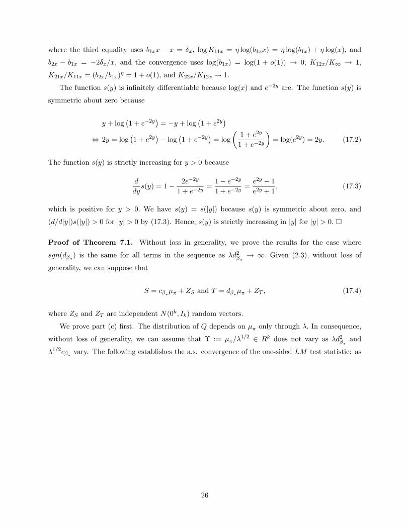
where the third equality uses b1xx x = x; logK11x = log(b1xx) = log(b1x) + log(x); and

b2x b1x = 2x=x; and the convergence uses log(b1x) = log(1 + o(1)) ! 0; K12x=K1 ! 1;

K21x=K11x = (b2x=b1x) = 1 + o(1); and K22x=K12x ! 1:

The function s(y) is innitely di¤erentiable because log(x) and e2y are. The function s(y) is

symmetric about zero because

y + log1 + e2y

= y + log

1 + e2y

, 2y = log

1 + e2y

log

1 + e2y

= log

1 + e2y

1 + e2y

= log(e2y) = 2y: (17.2)

The function s(y) is strictly increasing for y > 0 because

d

dys(y) = 1 2e2y

1 + e2y=1 e2y1 + e2y

=e2y 1e2y + 1

; (17.3)

which is positive for y > 0: We have s(y) = s(jyj) because s(y) is symmetric about zero, and(d=djyj)s(jyj) > 0 for jyj > 0 by (17.3). Hence, s(y) is strictly increasing in jyj for jyj > 0:

Proof of Theorem 7.1. Without loss in generality, we prove the results for the case where

sgn(d) is the same for all terms in the sequence as d2! 1: Given (2.3), without loss of

generality, we can suppose that

S = c + ZS and T = d + ZT ; (17.4)

where ZS and ZT are independent N(0k; Ik) random vectors.

We prove part (c) rst. The distribution of Q depends on only through : In consequence,

without loss of generality, we can assume that := =1=2 2 Rk does not vary as d2 and

1=2c vary. The following establishes the a.s. convergence of the one-sided LM test statistic: as

26

d2 !1 and 1=2c ! c1;

QST

Q1=2T

=(c + ZS)

0(d + ZT )

((d + ZT )0(d + ZT ))

1=2

=(c + ZS)

0(d + ZT )

(d2)1=2(1 + oa:s:(1))

=(c=

1=2 + ZS=1=2)0(sgn(d) +Oa:s:(1=jd j)(1 + oa:s:(1))

=

sgn(d)

0ZS + sgn(d)1=2c +Oa:s:

(c2)

1=2

(d2)1=2

!+Oa:s:

1

(d2)1=2

!!(1 + oa:s:(1))

!a:s: sgn(d)0ZS + sgn(d)c1

= : LM11 N(sgn(d)c1; 1); (17.5)

where the rst equality holds by (3.1) and (17.4), the second equality holds using d + ZT =

(d2)1=2(d=(d

2)1=2 + oa:s:(1)) since d2 ! 1; the convergence holds because d2 ! 1

and 1=2c ! c1; and the limit random variable LM11 has a N(sgn(d)c1; 1) distribution

because sgn(d)0ZS N(0; 1) (since ZS N(0k; Ik) and jjjj = 1):

The a.s. convergence in (17.5) implies convergence in distribution by the dominated convergence

theorem applied to 1(QST =Q1=2T y) for any xed y 2 R: In consequence, we have

P (LM > 21;1) = P ((QST =Q1=2T )2 > 21;1)! P (LM2

11 > 21;1) = P (21(c21) > 21;1)

(17.6)

as d2 !1 and 1=2c ! c1; which establishes part (c).

To prove Theorem 7.1(a), we apply Lemma 17.1 to a realization of the random vectors ZS and

ZT with

x := (d2QT )1=2;

b1xx := ((Q;0;))1=2 := 1=2(c2QS + 2cdQST + d

2QT )

1=2;

b2xx := 1=2(c2QS 2cdQST + d2QT )

1=2;

K11x := (b1xx)(k1)=2;

K12x :=(b1xx)

1=2I(k2)=2(b1xx)

eb1xx

K21x := (b2xx)(k1)=2; and

K22x :=(b2xx)

1=2I(k2)=2(b2xx)

eb2xx; (17.7)

27

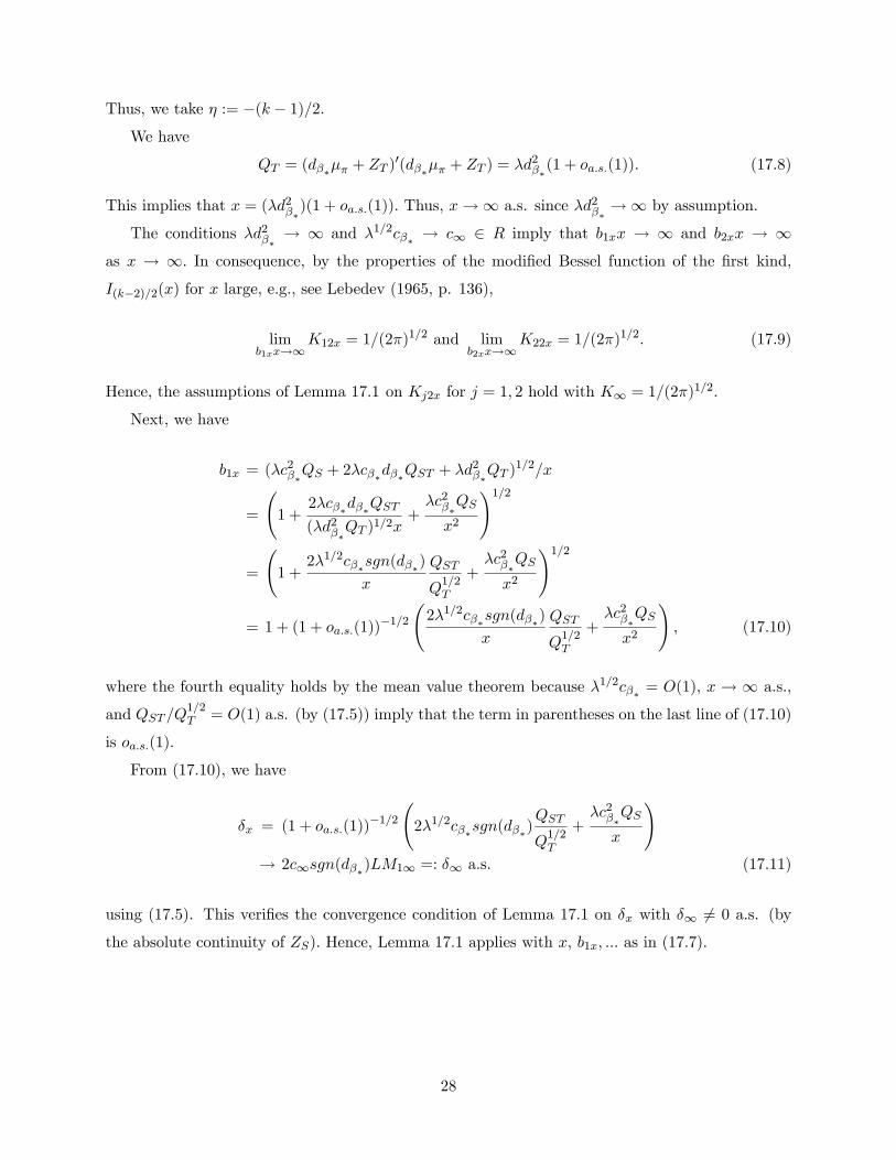
Thus, we take := (k 1)=2:We have

QT = (d + ZT )0(d + ZT ) = d2(1 + oa:s:(1)): (17.8)

This implies that x = (d2)(1 + oa:s:(1)): Thus, x!1 a.s. since d2 !1 by assumption.

The conditions d2 ! 1 and 1=2c ! c1 2 R imply that b1xx ! 1 and b2xx ! 1as x ! 1: In consequence, by the properties of the modied Bessel function of the rst kind,I(k2)=2(x) for x large, e.g., see Lebedev (1965, p. 136),

limb1xx!1

K12x = 1=(2)1=2 and lim

b2xx!1K22x = 1=(2)

1=2: (17.9)

Hence, the assumptions of Lemma 17.1 on Kj2x for j = 1; 2 hold with K1 = 1=(2)1=2:

Next, we have

b1x = (c2QS + 2cdQST + d2QT )

1=2=x

=

1 +

2cdQST

(d2QT )1=2x

+c2QS

x2

!1=2

=

1 +

21=2csgn(d)

x

QST

Q1=2T

+c2QS

x2

!1=2

= 1 + (1 + oa:s:(1))1=2

21=2csgn(d)

x

QST

Q1=2T

+c2QS

x2

!; (17.10)

where the fourth equality holds by the mean value theorem because 1=2c = O(1); x ! 1 a.s.,

and QST =Q1=2T = O(1) a.s. (by (17.5)) imply that the term in parentheses on the last line of (17.10)

is oa:s:(1):

From (17.10), we have

x = (1 + oa:s:(1))1=2

21=2csgn(d)

QST

Q1=2T

+c2QS

x

!! 2c1sgn(d)LM11 =: 1 a.s. (17.11)

using (17.5). This veries the convergence condition of Lemma 17.1 on x with 1 6= 0 a.s. (by

the absolute continuity of ZS): Hence, Lemma 17.1 applies with x; b1x; ::: as in (17.7).

28

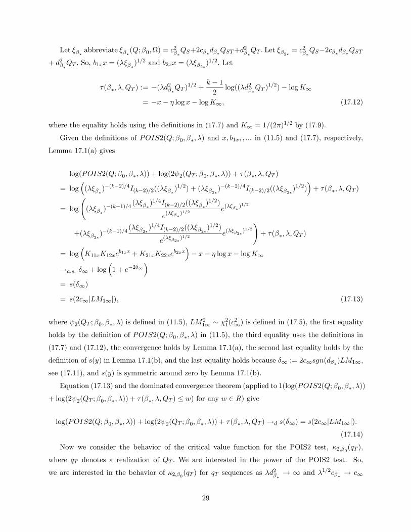
Let abbreviate (Q;0;) = c2QS+2cdQST+d2QT : Let 2 = c2QS2cdQST

+ d2QT : So, b1xx = ()1=2 and b2xx = (2)

1=2: Let

(; ;QT ) := (d2QT )1=2 +

k 12

log((d2QT )1=2) logK1

= x log x logK1; (17.12)

where the equality holds using the denitions in (17.7) and K1 = 1=(2)1=2 by (17.9).

Given the denitions of POIS2(Q;0; ; ) and x; b1x; ; ::: in (11.5) and (17.7), respectively,

Lemma 17.1(a) gives

log(POIS2(Q;0; ; )) + log(2 2(QT ;0; ; )) + (; ;QT )

= log()

(k2)=4I(k2)=2(()1=2) + (2)

(k2)=4I(k2)=2((2)1=2)

+ (; ;QT )

= log

()

(k1)=4 ()1=4I(k2)=2(()

1=2)

e( )1=2

e( )1=2

+(2)(k1)=4 (2)

1=4I(k2)=2((2)1=2)

e(2 )1=2

e(2 )1=2

!+ (; ;QT )

= logK11xK12xe

b1xx +K21xK22xeb2xx x log x logK1

!a:s: 1 + log1 + e21

= s(1)

= s(2c1jLM11j); (17.13)

where 2(QT ;0; ; ) is dened in (11.5), LM211 21(c

21) is dened in (17.5), the rst equality

holds by the denition of POIS2(Q;0; ; ) in (11.5), the third equality uses the denitions in

(17.7) and (17.12), the convergence holds by Lemma 17.1(a), the second last equality holds by the

denition of s(y) in Lemma 17.1(b), and the last equality holds because 1 := 2c1sgn(d)LM11;

see (17.11), and s(y) is symmetric around zero by Lemma 17.1(b).

Equation (17.13) and the dominated convergence theorem (applied to 1(log(POIS2(Q;0; ; ))

+ log(2 2(QT ;0; ; )) + (; ;QT ) w) for any w 2 R) give

log(POIS2(Q;0; ; )) + log(2 2(QT ;0; ; )) + (; ;QT )!d s(1) = s(2c1jLM11j):(17.14)

Now we consider the behavior of the critical value function for the POIS2 test, 2;0(qT );

where qT denotes a realization of QT : We are interested in the power of the POIS2 test. So,

we are interested in the behavior of 2;0(qT ) for qT sequences as d2! 1 and 1=2c ! c1

29

that are generated when the true parameters are (; ): This behavior is given in (17.8) to be

qT = d2(1 + o(1)) a.s. under (; ):

Up to this point in the proof, the parameters (; ) have played a duel role. First, they denote

the parameter values against which the POIS2 test is designed to have optimal two-sided power

and, hence, determine the form of the POIS2 test statistic. Second, they denote the true values

of and (because we are interested in the power of the POIS2 test when the (; ) values for

which it is designed are the true values). Here, where we discuss the behavior of the critical value

function 2;0(); (; ) only play the former role. The true value of is 0 and the true value of we denote by 0: The function 2;0() depends on (; ) because the POIS2 test statistic does,but the null distribution that determines 2;0() does not depend on (; ): In spite of this, thevalues qT which are of interest to us, do depend on (; ) as noted in the previous paragraph.

The function 2;0() is dened in (11.6). Its denition depends on the conditional null distribu-tion of Q1 given QT = qT whose density fQ1jQT (jqT ) is given in (11.3). This density depends on k;but not on any other parameters, such as 0; 0 = 000 ; or : In consequence, for the purposes

of determining the properties of 2;0() we can suppose that 0 = 0; 0 = 1k=jj1kjj; 0 = 1; and

= I2: In this case,

S = ZS N(0k; Ik); T = 0 + ZT N(0 ; Ik); (17.15)

and S and T are independent (using d0(0;) = b00b0(b00b0)

1=2 det()1=2 = 1 since b0 =

(1; 0)0 = (1; 0)0):

We now show that 2;0(qT ) satises

log(2;0(qT )) + log(2 2(qT ;0; ; )) + (; ; qT )! s(2jc1j(21;1)1=2) as qT !1 (17.16)

for any sequence of constants qT = d2(1 + o(1)) as d2!1:

Suppose random variables fWm : m 1g and W satisfy: (i) Wm !d W as m ! 1; (ii)W has a continuous and strictly increasing distribution function at its 1 quantile 1; and

(iii) P (Wm > m) = for all m 1 for some constants fm : m 1g: Then, m ! 1:

This holds because if lim supm!1 m > 1; then there is a subsequence fvmg of fmg such thatlimm!1 vm = 1+ > 1 and = P (Wvm > vm)! P (W > 1+) < P (W > 1) = ; which is

a contradiction, and likewise lim infm!1 m < 1 leads to a contradiction.

We apply the result in the previous paragraph with (a) fWm : m 1g given by log(POIS2(Q;0;; )) + log(2 2(qT ;0; ; )) + (; ; qT ) under the null hypothesis and conditional on T = t

with t = 1kq1=2T =k1=2 for some sequence of constants qT = d2(1 + o(1)) ! 1 as d2 !

30

1; (b) W = s(2c1jS01k=k1=2j); where S01k=k1=2 N(0; 1); (c) m equal to log(2;0(qT )) +

log(2 2(qT ;0; ; )) + (; ; qT ); and (d) 1 = s(2jc1j(21;1)1=2):We need to show conditions (i)-(iii) above hold. Condition (ii) holds straightforwardly for W

as in (b) given the normal distribution of S; the functional form of s(y); and c1 6= 0:By denition of 2;0(qT ); under the null hypothesis, PQ1jQT (POIS2(Q;0; ; ) > 2;0(qT )

jqT ) = for all qT 0; see (11.6). This implies that the invariant POIS2 test is similar. In turn,this implies that under the null hypothesis P (POIS2(Q;0; ; ) > 2;0(qT )jT = t) = for all

t 2 Rk because Theorem 1 of Moreira (2009) shows that any invariant similar test has null rejectionprobability conditional on T: This veries condition (iii) because the log function is monotone

and the last two summands of Wm and m dened in (a) and (c) above cancel.

Next, we show that condition (i) holds. Given (17.15) and t = 1kq1=2T =k1=2; under the null and

conditional on T = t; we have

QST

Q1=2T

=S0t

(t0t)1=2= S01k=k1=2 21; (17.17)

which does not depend on d2 or 1=2c : Hence, in place of the a.s. convergence result for

QST =Q1=2T as d2 !1 and 1=2c!c1 in (17.5), which applies under the alternative hypothesis

with true parameters (; ); we have QST =Q1=2T = S01k=k1=2 under the null hypothesis for all d2

and 1=2c : Using this in place of (17.5), the unconditional a.s. convergence result in (17.13),

established in (17.7)-(17.13), goes through as a conditional on T = t a.s. result without any further

changes. In consequence, the convergence in distribution result in (17.14) also holds conditional on

T = t a.s., but with s(2c1jS01k=k1=2j) in place of s(2c1jLM11j): This veries condition (i).Given that conditions (i)-(iii) hold, we obtain m ! 1 as d2 ! 1 for m and 1 dened

in (c) and (d), respectively, above. This establishes (17.16).

Given (17.16), we have

P;0;;(POIS2(Q;0; ; ) > 2;0(QT ))

= P;0;;(log(POIS2(Q;0; ; )) + log(2 2(QT ;0; ; )) + (; ;QT )

> log(2;0(QT )) + log(2 2(QT ;0; ; )) + (; ;QT ))

!d P (s(2c1jLM11j) > s(2c1j21;1j))

= P (LM211 > 21;1)

= P (21(c21) > 21;1); (17.18)

31

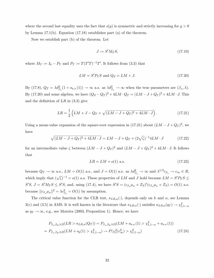
where the second last equality uses the fact that s(y) is symmetric and strictly increasing for y > 0

by Lemma 17.1(b). Equation (17.18) establishes part (a) of the theorem.

Now we establish part (b) of the theorem. Let

J := S0MTS; (17.19)

where MT := Ik PT and PT := T (T 0T )1T 0: It follows from (3.3) that

LM = S0PTS and QS = LM + J: (17.20)

By (17.8), QT = d2(1 + oa:s:(1)) ! 1 a.s. as d2 ! 1 when the true parameters are (; ):

By (17.20) and some algebra, we have (QS QT )2+4LM QT = (LM J +QT )2+4LM J: Thisand the denition of LR in (3.3) give

LR =1

2

LM + J QT +

p(LM J +QT )2 + 4LM J

: (17.21)

Using a mean-value expansion of the square-root expression in (17.21) about (LM J +QT )2; wehave p

(LM J +QT )2 + 4LM J = LM J +QT + (2p)14LM J (17.22)

for an intermediate value between (LM J +QT )2 and (LM J +QT )

2 + 4LM J: It followsthat

LR = LM + o(1) a.s. (17.23)

because QT ! 1 a.s., LM = O(1) a.s., and J = O(1) a.s. as d2 ! 1 and 1=2c ! c1 2 R;which imply that (

p)1 = o(1) a.s. These properties of LM and J hold because LM = S0PTS

S0S; J = S0MTS S0S; and, using (17.4), we have S0S = (c + ZS)0(c + ZS) = O(1) a.s.

because jjcjj2 = c2 = O(1) by assumption.

The critical value function for the CLR test, LR;(); depends only on k and ; see Lemma3(c) and (3.5) in AMS. It is well known in the literature that LR;() satises LR;(qT )! 21;1

as qT !1; e.g., see Moreira (2003, Proposition 1). Hence, we have

P;0;;(LR > LR;(QT )) = P;0;;(LM + oa:s:(1) > 21;1 + oa:s:(1))

= P;0;;(LM + op(1) > 21;1)! P (21(c21) > 21;1) (17.24)

32

as d2 ! 1 and 1=2c ! c1; where the rst equality holds by (17.23), QT ! 1 a.s. by

(17.8), and limqT!1 LR;(qT ) = 21;1 and the convergence holds by part (c) of the theorem.

This establishes part (b) of the theorem.

Proof of Theorem 7.2. First, we establish part (a)(i) of the theorem. By (11.8) with =

and = ; we have

(;) =

24 !21 !12

!12 !22

35 =24 2u + 2uv +

2v2 uv +

2v

uv + 2v 2v

35 : (17.25)

Using this, we obtain, as uv ! 1;

c = c(0;(;)) = ( 0)(!21 20!12 + !2220)1=2

= ( 0)(2u + 2uv + 2v2 20(uv + 2v) + 2v20)1=2

= ( 0)(2u + 2( 0)uvuv + ( 0)22v)1=2

! ( 0)(2u 2( 0)uv + ( 0)22v)1=2

= ( 0)=ju ( 0)vj; (17.26)

where the second equality uses (2.3), the convergence only holds if u ( 0)v 6= 0; and thefourth equality uses uv = uvuv: This proves part (a)(i).

To prove part (a)(ii), we have

d = d(0;(;)) = b0b0(b00b0)

1=2 det()1=2 (17.27)

= (!21 !12(0 + ) + !220) (!21 20!12 + !2220)1=2 (!21!22 !212)1=2;

where the second equality holds by (2.3). The second multiplicand on the rhs of (17.27) converges

to ju ( 0)vj1 provided u ( 0)v 6= 0 by the calculations in (17.26).The rst multiplicand on the rhs of (17.27) satises, as uv ! 1;

!21 !12(0 + ) + !220

= 2u + 2uv + 2v2 (uv + 2v)(0 + ) + 2v0

= 2u + uvuv( 0)

! u(u v( 0)); (17.28)

33

where the rst equality uses (17.25) and the second equality holds by simple algebra and uv =

uvuv:

The reciprocal of the square of the third multiplicand on the rhs of (17.27) satises, as uv ! 1;

!21!22 !212 = (2u + 2uvuv +

2v2)

2v (uvuv + 2v)2

! (2u 2uv + 2v2)2v (uv + 2v)2

= (u v)22v (u + v)22v

= 0; (17.29)

where the rst equality holds by (17.25) and uv = uvuv:

Combining (17.27)-(17.29) and > 0 proves part (a)(ii).

Next, we establish part (b) of the theorem. Using the denition of c(0;) in (2.3), we have

lim!1

c(0;) = lim!1

( 0)(b00b0)1=2

= lim!1

( 0)(!21 20!1!2 + !2220)1=2

= ( 0)=j!1 !20j; (17.30)

where the third equality holds provided !1!20 6= 0: This establishes part (b)(i) of the theorem.Using the denition of d(0;) in (2.3) and b := (1; )

0; we have

lim!1

d(0;) = lim!1

b0b0(b00b0)

1=2 det()1=2

= lim!1

(!21 !1!2(0 + ) + !220) (!21 20!1!2 + !2220)1=2

(!21!22 !21!222)1=2

= (!1 !20)(!1 !2) 1

j!1 !20j 1

!1!2 lim!1

1

(1 2)1=2= sgn((!1 !20)(!1 !2)) 1; (17.31)

where the third and fourth equalities hold provided !1 !20 6= 0 and !1 !2 6= 0: This and > 0 establish part (b)(ii) of the theorem.

Part (c)(i) is proved as follows:

c = 0

(2u + 2( 0)uvuv + ( 0)22v)1=2! 1

vas (uv; 0)! (1;1); (17.32)

where the rst equality holds by (17.26) and the convergence holds by considering only the dominant

0 terms. The same result holds as (uv; 0)! (1;1) because uv enters the middle expression

34

in (17.32) only through a term that does not a¤ect the limit.

Part (c)(ii) is proved using the expression for d in (17.27). By (17.29), the third multiplicand

in (17.27), which does not depend on 0; diverges to innity when uv ! 1 or 1: The product ofthe rst two multiplicands on the rhs of (17.27) equals

!21 !12(0 + ) + !220(!21 20!12 + !2220)1=2

=2u + uvuv( 0)

(2u + 2( 0)uvuv + ( 0)22v)1=2

! uvv

= u as (uv; 0)! (1;1); (17.33)

where the equality uses the calculations in the rst three lines of (17.26) and (17.28) and the

convergence holds by considering only the dominant 0 terms. When (uv; 0) ! (1;1); thelimit in (17.33) is u because uv enters multiplicatively in the dominant 0 term in the numerator.In both cases, the product of the rst two multiplicands on the rhs of (17.27) converges to a non-

zero constant and the third multiplicand diverges to innity. Hence, d diverges to +1 or 1and d2 !1 since > 0; which completes the proof.

Part (d)(i) holds because

c = 0

(!21 20!1!2 + !2220)1=2! 1

!2as (; 0)! (1;1); (17.34)

where the equality uses (17.30). The same convergence holds as (; 0) ! (1;1) because uventers the middle expression in (17.34) only through a term that does not a¤ect the limit.

Part (d)(ii) is proved using the expression for d in (17.31):

d =(!21 !1!2(0 + ) + !220)(!21 20!1!2 + !2220)1=2

(!21!22 !21!222)1=2;

(!21 !1!2(0 + ) + !220)(!21 20!1!2 + !2220)1=2

! (!22 !1!2)!2

= (!1 !2); and

(!21!22 !21!222)1=2 !1 as (; 0)! (1;1): (17.35)

Hence, d2 !1 as (; 0)! (1;1) provided !1!2 6= 0:When (; 0)! (1;1); thelimit in the second line of (17.35) is (!22 + !1!2)=!2 = (!1 + !2) and, hence, d

2! 1

provided !1 + !2 6= 0; which completes the proof.

35

18 Proofs of Theorem 12.1 and Lemmas 13.1 and 13.2

Proof of Theorem 12.1. By Cor. 2 and Comment 2 to Cor. 2 of Andrews, Moreira, and Stock

(2004), for all (; 0; ;);

P;0;;(0(Q) = 1) P;0;;(POIS(Q;0; ) > 0(QT )): (18.1)

That is, the test on the rhs is the (one-sided) POIS test for testing H0 : = 0 versus H1 : =

for xed known and any 0 under H1:We use the dominated convergence theorem (DCT) to show

lim0!1

P;0;;(POIS(Q;0; ) > 0(QT )) = Puv ;v(POIS(Q;1; uv) > 1(QT )): (18.2)

Equations (18.1) and (18.2) imply that the result of Theorem 12.1 holds.

By (12.2), (12.5), and Lemma 14.1(b) and (e),

lim0!1

POIS(q;0; ) = POIS(q;1; uv) (18.3)

for all 2 2 variance matrices q; for given (; ;):The proof of (18.2) is the same as the proof of Lemma 16.1(a), but with POIS(Q;0; );

0(QT ); POIS(Q;1; uv); and 1(QT ) in place of POIS2(Q;0; ; ); 2;0(QT ); POIS2(Q;1;juvj; v); and 2;1(QT ); respectively, using (18.3) in place of (16.6), and using the results (estab-lished below) that (i) the Lebesgue measure of the set of (qS ; qST ; qT ) for which POIS(q;1; uv) =1(qT ) is zero, (ii) PQ1jQT (POIS(Q;1; uv) = xjqT ) = 0 for all qT 0; and (iii) the distributionfunction of POIS(Q;1; uv) is strictly increasing at its 1 quantile 1(qT ) under PQ1jQT (jqT )for all qT 0:

Condition (i) holds because (a) POIS(q;1; uv) = qS + 2ruvqST (see (12.5)) implies that the

Lebesgue measure of the set of (qS ; qST ) for which qS +2ruvqST = 1(qT ) is zero for all qT and (b)

the Lebesgue measure of the set of (qS ; qST ; qT ) for which qS + 2ruvqST = 1(qT ) is obtained by

integrating the set in (a) over qT 2 R subject to the constraint that q is positive denite.

Condition (ii) holds by the absolute continuity of POIS(Q;1; uv) under PQ1jQT (jqT ) (by thefunctional form of POIS(Q;1; uv) and the absolute continuity of Q1 under PQ1jQT (jqT ); whosedensity is given in (11.3)).

Condition (iii) holds because we can write POIS(Q;1; uv) = S0S+2ruvS0T = (S+ruvT )0(S+

ruvT ) r2uvT0T; where [S : T ] has a multivariate normal distribution with means matrix given by

(5.2) and identity variance matrix and, hence, POIS(Q;1; uv) has a shifted noncentral 2 distri-

36

bution conditional on T = t: In consequence, it has a positive density on (r2uvt0t;1) = (r2uvqT ;1)

conditional on T = t and also conditional on QT = qT (because the latter conditional density is the

integral of the former conditional density over t such that t0t = qT ): This completes the proof.

Proof of Lemma 13.1. First, we show that (13.4) implies the equation for 2 in (13.2). By the

expression d = a01a0(a001a0)1=2 given in (2.7) in AMS, where a := (; 1)0 and a0 := (0; 1)

0;

for any 2 R;

d d0 = (a a0)01a0(a001a0)1=2

= ( 0)e011a0(a001a0)1=2 := ( 0)r0 ; (18.4)

where e1 := (1; 0)0 and the last equality holds by the denition of r0 :

Substituting (18.4) into the second equation in (13.4) gives

1=22 d2 =

1=2d

i¤ 1=22 (d0 + r0(2 0)) = 1=2(d0 + r0( 0))

i¤ 1=22 d0 = 1=2(d0 + r0( 0)) r0

1=22 (2 0): (18.5)

Given the denition of c in (2.3), the rst equation in (13.4) can be written as

1=22 (2 0) = 1=2( 0): (18.6)

Substituting this into (18.5) yields

1=22 d2 =

1=2d

i¤ 1=22 d0 = 1=2(d0 + 2r0( 0))

i¤ 1=22 = 1=2d0 + 2r0( 0)

d0: (18.7)

The square of the equation in the last line in (18.7) is the equation for 2 in (13.2).

Next, we show that (13.4) implies the equation for 2 in (13.2). Using (18.6), the rst equation

in (13.4) can be written as

2 = 0 1=2

1=22

( 0): (18.8)

37

This combined with the equation for 1=2=1=22 obtained from the last line of (18.7) gives

2 = 0 d0

d0 + 2r0( 0)( 0); (18.9)

where a minus sign appears because the sign in (18.8) gets multiplied by the sign in the last

line of (18.7), which yields a minus sign in both cases. Equation (18.9) is the same as the rst

condition in (13.2). This completes the proof that (13.4) implies (13.2).

Now, we prove the converse. We suppose (13.2) holds. Taking the square root of the second

equation in (13.2) gives

1=22 = 1=2

d0 + 2r0( 0)d0

; (18.10)

where the sign means that this equation holds either with + or with : Substituting this intothe rst equation in (13.2) gives (18.8), which is the same as (18.6), and (18.6) is the rst equation

in (13.4).

The second equation in (13.4) is given by (18.5). Given that the rst equation in (13.4) holds,

the second equation in (13.4) is given in (18.7). The last line of (18.7) holds by (18.10). This

completes the proof that (13.2) implies (13.4).

Proof of Lemma 13.2. The proof of part (a) of the lemma is essentially the same as that of

Theorem 8(b) in AMS. The only change is to note that when (2; 2) satises (13.3), we have

= 2; = 2; and max = jj = j2j (using the notation in AMS). Because max = jj = j2j;

we obtainp2

q2max = 0 and the remainder of the proof of Theorem 8(b) goes through as is.

The proof of part (b) of the lemma is quite similar to the proof of Theorem 8(c) of AMS. The

latter proof rst considers the case where (2; 2) does not satisfy the second condition of (13.1).

This needs to be changed to (2; 2) does not satisfy the second condition of (13.1) or (13.3).

With this change, the rest of that part of the proof of Theorem 8(c) goes through unchanged.

The remaining cases (where both (13.1) and (13.3) fail) to consider are (i) when the second

condition in (13.1) holds and the rst condition in (13.1) fails and (ii) when the second condition in

(13.3) holds and the rst condition in (13.3) fails. These are mutually exclusive scenarios because

the second conditions in (13.1) and (13.3) are incompatible. The proof of Theorem 8(c) of AMS

considers case (i) and proves the result of Theorem 8(c) for that case. The proof of Theorem 8(c)

for case (ii) is quite similar to that for case (i) using (A.21) in AMS because = 2; max =jj = j2j > 0; and 6= 2 imply that sgn(

) = sgn(2) and sgn() 6= 2sgn(2): This lastinequality shows that the expression in (A.21) in AMS is a continuous function of QSTQ

1=2T that

is not even. (Note that (A.21) in AMS has a typo: the quantity 2sgn() in its second summand

38

should be 2sgn(2):)

19 Power Against Distant Alternatives Compared to Distant Null

Hypotheses

19.1 Scenario 1 Compared to Scenario 2

In this section, we consider the power properties of tests when j0j is large, where denotesthe true value of :We compare scenario 1, where 0 is xed and takes on large (absolute) values,

to scenario 2, where is xed and 0 takes on large (absolute) values. Scenario 1 yields the power

function of a test against distant alternatives. Scenario 2 yields the false coverage probabilities of

the CS constructed using the test for distant null hypotheses (from the true parameter value ).

We show that, while power goes to one in scenario 1 as ! 1 for xed 0; it is not true that

power goes to one in scenario 2 as 0 ! 1 for xed :

It is convenient to consider the AR test, which is the simplest test. The AR test rejects

H0 : = 0 when S0S > 2k;: When the true value is ; the distribution of the S

0S statistic is

noncentral 2 with noncentrality parameter

c2(0;) (19.1)

and k degrees of freedom. For the xed null hypothesis H0 : = 0; xed ; and xed ; the

power at the alternative hypothesis value is determined by c2(0;): We have

limjj!1

c2(0;) = limjj!1

( 0)2 (b00b0)1 =1: (19.2)

Hence, the power of the AR test goes to one as jj ! 1:On the other hand, if one xes the alternative hypothesis value and one considers the limit

as j0j ! 1; then one obtains

limj0j!1

c2(0;) = limj0j!1

( 0)2 (b00b0)1

= limj0j!1

( 0)2 (!21 2!120 + !2220)1

= 1=!22: (19.3)

Hence, the power of the AR test does not go to one as j0j ! 1 even though j0 j ! 1:The di¤ering results in (19.2) and (19.3) is easy to show for the AR test, but it also holds for

39

Kleibergens and Moreiras LM test and Moreiras CLR test. The numerical power function and

power envelope calculations in AMS are all of the type in scenario 1 in (19.2). The di¤erence in

the power of the AR (and other) tests between (19.2) and (19.3) suggests that it is worth exploring

the properties of tests in scenarios of the latter type as well. We do this in the paper and show

that the nding of AMS that the CLR test is essentially on the two-sided AE power envelope and

is always at least as powerful as the AR test does not hold when one considers a broader range of

null and alternative hypothesis values (0; ) than considered in the numerical results in AMS.

19.2 Structural Error Variance Matrices under Distant

Alternatives and Distant Null Hypotheses

Here, we compute the structural error variance matrices in scenarios 1 and 2 considered in (19.2)

and (19.3). By design, the reduced-form variance matrix is the same for 0 and and, hence,

does not vary between these two scenarios.

In scenario 1 in (19.2), the structural error variance matrix under H0 is (0;); dened in

(11.9). Under H1 : = ; as jj ! 1; we have

lim!1

uv(;) = lim!1

!12 !22(!21 2!12 + !222)1=2!2

= 1 and

limjj!1

2u(;)=2v(;) =

!21 2!12 + !222!22

=1; (19.4)

where uv(;); 2u(;); and

2v(;) are dened just below (11.9). Equation (19.4) shows

that, for standard power envelope calculations, when the alternative hypothesis value is large in

absolute value the structural variance matrix under H1 exhibits correlation close to one in absolute

value and a large ratio of structural to reduced-form variances.

In scenario 2 in (19.3), the structural error variance error matrix under H is (;): Under

H0 : = 0; by exactly the same argument as in (19.4) with 0 in place of ; we obtain

lim0!1

uv(0;) = 1 and limj0j!1

2u(0;)=2v(0;) =1: (19.5)

So, in scenario 2, when the null hypothesis value 0 is large in absolute value the structural variance

matrix under H0 exhibits correlation close to one in absolute value and a large ratio of structural

to reduced-form variances.

From a testing perspective, it is natural and time honored to x the null hypothesis value 0

and consider power as the alternative hypothesis value varies. On the other hand, a condence

set is the set of null hypothesis values 0 for which one does not reject H0 : = 0: Hence, for a

40

given true value ; the false coverage probabilities of the condence set equal one minus its power

as one varies H0 : = 0: Thus, from the condence set perspective, it is natural to x and

consider power as 0 varies.

20 Transformation of the 0 Versus Testing Problem

to a 0 Versus Testing Problem

In this section, we transform the general testing problem of H0 : = 0 versus H1 : =

for 2 Rk and xed to a testing problem of H0 : = 0 versus H1 : = for some 2 Rk

and some xed whose diagonal elements equal one. This is done using the transformations given

footnotes 7 and 8 of AMS, which argue that there is no loss in generality in the AMS numerical

results to take !21 = !22 = 1 and 0 = 0: These results help link the numerical work done in this

paper with that done in AMS.

Starting with the model in (2.1), we transform the model based on (y1; y2) with parameters

(; ) and xed reduced-form variance matrix to a model based on (ey1; y2) with parameters(e; ) and xed reduced-form variance matrix e; where

ey1 := y1 y20;e := 0; and

e := V ar

0@0@ ey1y2

1A1A = V ar

0@24 1 00 1

350@ y1

y2

1A1A=

24 !21 2!120 + !2220 !12 !220!12 !220 !22

35 : (20.1)

The transformed testing problem is H0 : e = 0 versus H1 : e = e; where e = 0; with

parameter and reduced-form variance matrix e:The matrix e does not have diagonal elements equal to one, so we transform the model based

on (ey1; y2) with parameters (e; ) and xed reduced-form variance matrix e to a model based on

41

(y1; y2) with parameters (; ) and xed reduced-form variance matrix ; where12

y1 :=ey1e!1 = y1 y20

(!21 2!120 + !2220)1=2

y2 :=1e!2 y2 = 1

!2y2;

:=e!2e!1 e = !2

(!21 2!120 + !2220)1=2( 0); and

:=1e!2 = 1

!2: (20.2)

In addition, we have

:= V ar

0@ y1

y2

1A = V ar

0@24 1=e!1 0

0 1=e!2350@ ey1

y2

1A1A=

24 1=e!1 0

0 1=e!235 e

24 1=e!1 0

0 1=e!235

=

24 1=e!1 0

0 1=!2

3524 !21 2!120 + !2220 !12 !220!12 !220 !22

3524 1=e!1 0

0 1=!2

35=

24 1!12!220

(!212!120+!2220)1=2!2

!12!220(!212!120+!22

20)1=2!2

1

35 : (20.3)

The transformed testing problem is H0 : = 0 versus H1 : = ; where

=!2

(!21 2!120 + !2220)1=2( 0); (20.4)

with parameter and reduced-form variance matrix :

Now, we consider the limit as 0 ! 1 of the original model and see what it yields in terms

of the transformed model. We have

lim0!1

= 1 and lim0!1

=

24 1 11 1

35 : (20.5)

So, the asymptotic testing problem as 0 ! 1 in terms of a model with a null hypothesis value

of 0 and a reduced-form variance matrix with ones on the diagonal is a test of H0 : = 0 versus

H1 : = 1:12The formula := (e!2=e!1)e in (20.2) comes from y1 := ey1=e!1 = (y2e+u)=e!1 = y2e=e!1+u=e!1 = (y2=e!2)e(e!2=e!1)

+ u=e!1 = y2 + u; where the last equality holds when := (e!2=e!1)e and u := u=e!1:42

We get the same expression for the limits as 0 ! 1 of c(0;) and d(0;) written in

terms of the transformed parameters (0; ; ;) as in Lemma 14.1 except they are multiplied by

v: This occurs because = =v: In consequence, the limits as 0 ! 1 of c(0;) and

d(0;) written in terms of the transformed parameters (0; ; ;) are the same as their

limits without any transformation.

Lemma 20.1 Let = (0) and = (0) be dened in (20.4) and (20.3), respectively. Let

0(0) = 0:

(a) lim0!1 c(0)(0(0);(0)) = 1:

(b) lim0!1 d(0)(0(0);(0)) =

uv(12uv)1=2

:

Comment. (i). By Lemmas 14.1 and 20.1, the distributions of all of the tests considered in this

paper are the same in the model in Section 2 when and are xed and the null hypothesis

value 0 satises 0 ! 1; and in the transformed model of this section when the null hypothesis0 is xed at 0 and the alternative hypothesis value = (0) and the reduced-form variance

= (0) converge as in (20.5) as 0 ! 1: (This uses the fact that v = 1 in Lemma 20.1.)(ii). AMS footnote 5 notes that there is a special parameter value = AR at which the one-

sided point optimal invariant similar test of H0 : = 0 versus H1 : = AR is the (two-sided) AR

test. In footnote 5 AR is dened to be AR =!21!120!12!220

: If we compute AR for the transformed

model (y1; y2) with parameters (; ;); where 0 = 0; we obtain

AR =!21 !120!12 !220

=1

!12= 1; (20.6)

which is the same as the limit of = (0) as 0 ! 1 in (20.2).

Proof of Lemma 20.1. First, we prove part (a). We have

c(0;) = ( 0)(b

00b0)

1=2

=!2

(!21 2!120 + !2220)1=2( 0)(1 2!120 +

20)1=2

=!2( 0)

(!21 2!120 + !2220)1=2! 1 as 0 ! 1; (20.7)

where the second equality uses (20.4) and the third equality uses 0 = 0: Hence, c(0;) !(1=v) as 0 ! 1 using the expression for in (20.2) and !2 = v:

43

Next, we prove part (b). Let b = (1;)0 and b0 = (1;0)0: We have

det() = 1 !212;

!12 =!12 !220

(!21 2!120 + !2220)1=2!2; and

b0b0(b

00b0)

1=2 =1 !120 !12 + 0(1 2!120 +

20)1=2

= 1 !12; (20.8)

where the second equality on the third line uses 0 = 0: Next, we have

1 !12 = 1 !12 !220(!21 2!120 + !2220)1=2!2

!2

(!21 2!120 + !2220)1=2( 0)

= 1 (!12 !220)( 0)

!21 2!120 + !2220

=!21 2!120 + !2220 !12 + !120 + !220 !2220

!21 2!120 + !2220

=!21 !120 !12 + !220

!21 2!120 + !2220; (20.9)

where the rst equality uses (20.3) and (20.4).

In addition, we have

1 !212 = 1 (!12 !220)2

(!21 2!120 + !2220)!22

=!21!

22 2!12!220 + !4220 !212 + 2!12!220 !420

(!21 2!120 + !2220)!22

=!21!

22 !212

(!21 2!120 + !2220)!22; (20.10)

where the rst equality uses (20.8).

Using (20.8)-(20.10), we have

d(0;) = b

0b0(b

00b0)

1=2 det()1=2

=!21 !120 !12 + !220

!21 2!120 + !2220

!21!

22 !212

(!21 2!120 + !2220)!22

1=2=

(!21 !120 !12 + !220)(!21 2!120 + !2220)1=2(!21!22 !212)1=2

!2: (20.11)

The rhs of (20.11) is the same as the expression on the second line of (14.2) multiplied by !2 = v:

In consequence, the calculations in (14.2)-(14.4) give the result of part (a) of Lemma 20.1.

44

21 Transformation of the 0 Versus Testing Problem

to a 0 Versus 0 Testing Problem

In this section, we transform the general testing problem of H0 : = 0 versus H1 : =

for 2 Rk and xed reduced-form variance matrix to a testing problem of H0 : = 0 versus

H1 : = 0 for some 2 Rk and some xed with diagonal elements equal to one. These

transformation results imply that there is no loss in generality in the numerical results of the paper

to taking !21 = !22 = 1 and = 0:We also show that there is no loss in generality in the numerical

results of the paper to taking uv 2 [0; 1]; rather than uv 2 [1; 1]; where uv is the structuralvariance matrix correlation dened in (4.5).

We consider the same transformations as in Section 20, but with in place of 0 in (20.1)-(20.3)

and with the roles of and 0 reversed in (20.4) and (20.5). The transformed testing problem

given the transformations in (20.1) (with in place of 0) is H0 : e = e0 versus H1 : e = 0; wheree0 = 0 ; with parameter and reduced-form variance matrix e: The transformed testingproblem given the transformations in (20.1)-(20.3) (with in place of 0) is H0 : = 0 versus

H1 : = 0; where e0 = 0 ; with parameters ; ; and dened in (20.2) and (20.3) (with

the roles of and 0 reversed).

For example, a scenario in which a typical test has high power in the original scenario of testing

H0 : = 0 versus H1 : = ; such as 0 = 0 and jj large, gets transformed into the testingproblem of H0 : = 0 versus H1 : = 0 with correlation !12 (the (1; 2) element of ) close to

1; because by (20.5) (with the roles of and 0 reversed) we have

lim!1

=

24 1 11 1

35 : (21.1)

In this case, we also have lim!1 0 = 1 by (20.5). Also, note that the reduced-form and

structural variances matrices are equal when the alternative hypothesis holds in the testing problem

H0 : = 0 versus H1 : = 0; so the result in (21.1) also applies to the structural variance matrix

(;) when = 0 whose correlation we denote by uv; i.e., lim!1 uv = 1: Here theparameter uv is the parameter uv that appears in the tables in the paper. These results are

useful in showing how the numerical results of the paper apply to general hypotheses of the form

H0 : = 0 versus H1 : = :

Next, we show that there is no loss in generality in the numerical results of the paper to taking

uv 2 [0; 1]: We consider the hypotheses H0 : = 0 versus H1 : = 0; as in the numerical results

in the paper. When the true equals 0 and has ones on its diagonal, the reduced-form and

45

structural variance matrices are equal, see (11.9). Hence, the correlation !12 given by equals the

structural variance correlation uv in power calculations in the paper, and it su¢ ces to show that

there is no loss in generality in the numerical results of the paper to taking !12 2 [0; 1]:By (2.3), the distributions of S and T only depend on c(0;); d(0;); and := (Z

0Z)1=2:

The vector does not depend on ; 0; or : First, note that !12 enters c(0;) := ( 0)(b

00b0)

1=2 = ( 0)(!21 2!120 + !22

20)1=2 only through !120: In consequence, the

distribution of S is the same under (0; !12) as under (0;!12): Second, by (2.8) of AMS,d(0;) can be written as b

0b0(b00b0)1=2 det()1=2; where b := (1;)0: The distribution of T

when = 0 depends on d0(0;) = (1!120)(b00b0)1=2 det()1=2: The rst two multiplicandsdepend on !12 only through !120 and the third multiplicand only depends on !12 through !

212

(because det() = 1 !212): In addition, S and T are independent. Hence, the distribution of

[S : T ] for given (0; !12) when = 0 equals its distribution under (0;!12) when = 0: Thus,the power of a test of H0 : = 0 versus H1 : = 0 when !12 < 0 equals its power for testing

H0 : = 0 versus H1 : = 0 for !12 > 0:

22 Additional Numerical Results

This section contains Tables SM-I,..., SM-V and Figure SM-I, which provide additional numer-

ical results to those in Tables I,..., V in the main paper.

Table SM-I is analogous to Table I, but considers AR and POIS1 CSs, in addition to the CLR

and POIS21 CSs. Here, POIS1 denotes the CS obtained from the optimal one-sided invariant

similar test as 0 ! 1 dened in (12.5) in Section 12.2. Table SM-I reports probabilities of innite

length, as well as di¤erences in probabilities of innite length (DPILs) for CLR and AR, AR and

POIS21; and CLR and POIS21 CSs. In addition, it reports simulation standard deviations for

the rst and third DPILs.

The results for the DPILs vary greatly with uv: When uv = 0; the AR CS is the same as

the optimal POIS1 CS and the CLR-AR DPILs range over [:001; :049] as (k; ) vary. On the

other hand, when uv = :9; the AR CS is far from optimal and the CLR-AR DPILs range over

[:002;:421] as (k; ) vary. In sum, when uv :5; the AR CS can, and typically does, perform

noticeably worse than the CLR CS in terms of DPILs.

Table SM-II reports more detailed results than those given in Table II. Table SM-II reports the

maximum power di¤erences (PDs) over 0 values between the POIS2 power envelope and the CLR

test for a grid of (k; uv; ) values. (In contrast, Table II reports maximum and average PDs over

(0; ) values for a grid of (k; uv) values.) Table SM-II shows that the maximum (over 0) PDs

46

vary substantially over values for uv :7 values and less so for uv = :9: For example, for k = 5

and uv = :0; :3; :5; :7; :9; the PDs ranges (over values) are [:004; :030]; [:008; :034]; [:007; :029];

[:005; :033]; [:001; :017]; respectively.

Tables SM-III and SM-IV are the same as Table II except they consider the AR and LM tests,

respectively, rather than the CLR test. As noted in the main paper, Tables SM-III and SM-IV

show that the power of the AR and LM tests is much farther from the POIS2 power envelope than

is the power of the CLR test. Table SM-III(a) shows that the maximum and average (over (0; ))

PDs for the AR test are increasing in k up to k = 20; but drop going from k = 20 to 40: (This

drop may be due to the choice of values considered. The choice yields the max value for the AR

test to be on the upper bound of the values considered.) Table SM-III(b) shows that the maximum

and average (over (0; )) PDs for the AR test are increasing in uv for all values of k; which is

the opposite of the pattern for the CLR test. Table SM-III(b) also shows that the max values are

at the boundary of the grid of values considered for all k:

Table SM-IV(a) shows that the maximum and average PDs (over (0; )) for the LM test are

clearly increasing in k; except that for uv = 0; :3 there is a drop from k = 20 to 40 (which may

be due to the choice of values considered, as for the AR test). Table SM-IV(b) shows that the

maximum and average (over (0; )) PDs for the LM test are decreasing in uv for all values of k;

as for the CLR test. Table SM-IV(b) also shows that the max values decrease in uv for each k;

as with the CLR test.

Table SM-V is the same as Table III except that it reports results for k = 2; 5; 10; 20; and 40;

rather than just k = 5: It also reports results for a ner grid of 0 values than in Table IV and it

reports the power of the WAP2 test, in addition to the di¤erence in power between the WAP2 and

CLR tests.

Figure SM-I provides graphs that are the same as in AMS, but with = 0; rather than = :5

or :95: Specically, these graphs provide the power of the signicance level :05 CLR, LM, and AR

tests and the POIS2 power envelope for xed null value 0 = 0; varying true value ; k = 2; 5; 10

and = 5; 20: The number of simulation repetitions used to construct the power functions is 5,000

and 100,000 repetitions are used to compute the null distribution of the POIS2 statistic to obtain

its p-values.

Figure SM-I shows that the power of the CLR test is very close to the POIS2 power envelope

in the scenarios considered. In fact, the maximum di¤erences are :0074; :0040; :0110; :0062; :0102;

and :0090 in the six graphs in Figure SM-I. Note that = 0 is the value that yields many of

the largest di¤erences between the power of the CLR test and the POIS2 power envelope when the

47

true = 0 is xed and the null value 0 varies, as shown in Tables II and SM-II.13 The results in

Figure SM-I show that standard power graphs with 0 = 0 xed and true varying, as in AMS,

do not pick up the relatively large di¤erences between the power of the CLR test and the POIS2

power envelope that appear in some = 0 parameter congurations considered in Tables II and

SM-II.

13 In Tables II and SM-II, uv = for all 0 values because the true value = 0:

48

References

Andrews, D. W. K., M. J. Moreira, and J. H. Stock (2004): Optimal Invariant Similar Tests for

Instrumental Variables Regression with Weak Instruments,Cowles Foundation Discussion

Paper No. 1476, Yale University.

(2006): Optimal Two-sided Invariant Similar Tests for Instrumental Variables Regres-

sion,Econometrica, 74, 715752.

Lebedev, N. N. (1965): Special Functions and Their Application. Englewood Cli¤s, NJ: Prentice-

Hall.

Mills, B., M. J. Moreira, and L. P. Vilela (2014): Tests Based on t-Statistics for IV Regression

with Weak Instruments,Journal of Econometrics, 182, 351363.

Moreira, M. J. (2009): Tests with Correct Size When Instruments Can Be Arbitrarily Weak,

Journal of Econometrics, 152, 131-140.

49

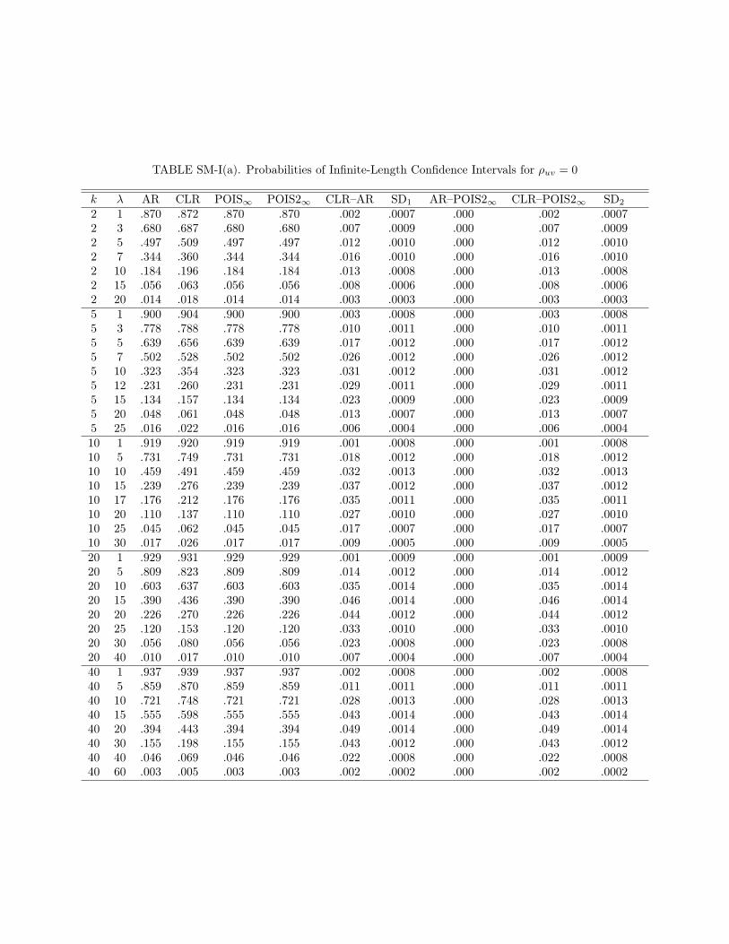
TABLE SM-I(a). Probabilities of Infinite-Length Confidence Intervals for ρuv = 0

k λ AR CLR POIS∞ POIS2∞ CLR–AR SD1 AR–POIS2∞ CLR–POIS2∞ SD2

2 1 .870 .872 .870 .870 .002 .0007 .000 .002 .00072 3 .680 .687 .680 .680 .007 .0009 .000 .007 .00092 5 .497 .509 .497 .497 .012 .0010 .000 .012 .00102 7 .344 .360 .344 .344 .016 .0010 .000 .016 .00102 10 .184 .196 .184 .184 .013 .0008 .000 .013 .00082 15 .056 .063 .056 .056 .008 .0006 .000 .008 .00062 20 .014 .018 .014 .014 .003 .0003 .000 .003 .00035 1 .900 .904 .900 .900 .003 .0008 .000 .003 .00085 3 .778 .788 .778 .778 .010 .0011 .000 .010 .00115 5 .639 .656 .639 .639 .017 .0012 .000 .017 .00125 7 .502 .528 .502 .502 .026 .0012 .000 .026 .00125 10 .323 .354 .323 .323 .031 .0012 .000 .031 .00125 12 .231 .260 .231 .231 .029 .0011 .000 .029 .00115 15 .134 .157 .134 .134 .023 .0009 .000 .023 .00095 20 .048 .061 .048 .048 .013 .0007 .000 .013 .00075 25 .016 .022 .016 .016 .006 .0004 .000 .006 .000410 1 .919 .920 .919 .919 .001 .0008 .000 .001 .000810 5 .731 .749 .731 .731 .018 .0012 .000 .018 .001210 10 .459 .491 .459 .459 .032 .0013 .000 .032 .001310 15 .239 .276 .239 .239 .037 .0012 .000 .037 .001210 17 .176 .212 .176 .176 .035 .0011 .000 .035 .001110 20 .110 .137 .110 .110 .027 .0010 .000 .027 .001010 25 .045 .062 .045 .045 .017 .0007 .000 .017 .000710 30 .017 .026 .017 .017 .009 .0005 .000 .009 .000520 1 .929 .931 .929 .929 .001 .0009 .000 .001 .000920 5 .809 .823 .809 .809 .014 .0012 .000 .014 .001220 10 .603 .637 .603 .603 .035 .0014 .000 .035 .001420 15 .390 .436 .390 .390 .046 .0014 .000 .046 .001420 20 .226 .270 .226 .226 .044 .0012 .000 .044 .001220 25 .120 .153 .120 .120 .033 .0010 .000 .033 .001020 30 .056 .080 .056 .056 .023 .0008 .000 .023 .000820 40 .010 .017 .010 .010 .007 .0004 .000 .007 .000440 1 .937 .939 .937 .937 .002 .0008 .000 .002 .000840 5 .859 .870 .859 .859 .011 .0011 .000 .011 .001140 10 .721 .748 .721 .721 .028 .0013 .000 .028 .001340 15 .555 .598 .555 .555 .043 .0014 .000 .043 .001440 20 .394 .443 .394 .394 .049 .0014 .000 .049 .001440 30 .155 .198 .155 .155 .043 .0012 .000 .043 .001240 40 .046 .069 .046 .046 .022 .0008 .000 .022 .000840 60 .003 .005 .003 .003 .002 .0002 .000 .002 .0002

TABLE SM-I(b). Probabilities of Infinite-Length Confidence Intervals for ρuv = .3

k λ AR CLR POIS∞ POIS2∞ CLR–AR SD1 AR–POIS2∞ CLR–POIS2∞ SD2

2 1 .869 .871 .863 .867 .002 .0007 .003 .004 .00072 3 .680 .682 .654 .679 .002 .0010 .001 .003 .00082 5 .497 .502 .463 .494 .005 .0010 .002 .008 .00092 7 .346 .349 .306 .344 .004 .0011 .002 .005 .00082 10 .185 .188 .152 .181 .003 .0009 .003 .006 .00072 15 .056 .057 .040 .053 .001 .0006 .002 .004 .00052 20 .015 .015 .009 .014 .000 .0004 .001 .001 .00035 1 .901 .903 .896 .900 .002 .0008 .000 .003 .00085 3 .778 .783 .759 .774 .005 .0011 .005 .010 .00105 5 .639 .649 .608 .636 .010 .0013 .003 .012 .00105 7 .502 .513 .462 .501 .011 .0013 .001 .012 .00105 10 .322 .332 .280 .316 .009 .0013 .006 .016 .00105 12 .231 .239 .192 .228 .008 .0012 .003 .011 .00095 15 .135 .139 .103 .126 .005 .0010 .008 .013 .00085 20 .048 .050 .033 .044 .002 .0007 .005 .007 .00055 25 .016 .016 .009 .014 .001 .0005 .002 .002 .000310 1 .918 .920 .914 .917 .002 .0009 .000 .002 .000810 5 .730 .740 .705 .726 .010 .0013 .005 .015 .001110 10 .459 .469 .412 .455 .010 .0014 .003 .014 .001110 15 .238 .248 .196 .228 .009 .0013 .010 .020 .001010 17 .177 .184 .138 .168 .007 .0012 .009 .017 .000910 20 .108 .114 .080 .100 .006 .0010 .008 .014 .000710 25 .045 .047 .028 .039 .002 .0007 .005 .008 .000510 30 .017 .018 .010 .014 .001 .0005 .003 .004 .000420 1 .929 .931 .928 .927 .002 .0008 .001 .003 .000820 5 .808 .817 .791 .806 .009 .0012 .002 .011 .001120 10 .602 .619 .562 .597 .016 .0015 .005 .022 .001220 15 .393 .406 .340 .381 .012 .0015 .013 .025 .001220 20 .227 .237 .180 .216 .009 .0013 .012 .021 .001020 25 .119 .126 .086 .110 .007 .0011 .009 .016 .000820 30 .056 .059 .036 .047 .003 .0009 .009 .012 .000620 40 .010 .011 .005 .007 .001 .0004 .003 .003 .000340 1 .938 .940 .935 .939 .001 .0008 -.000 .001 .000840 5 .860 .867 .848 .858 .007 .0011 .001 .008 .001040 10 .718 .735 .691 .715 .017 .0014 .002 .020 .001240 15 .554 .570 .509 .547 .016 .0015 .007 .022 .001240 20 .392 .409 .337 .380 .017 .0016 .012 .029 .001240 30 .154 .163 .114 .143 .009 .0013 .012 .021 .000940 40 .045 .049 .028 .037 .004 .0008 .008 .012 .000640 60 .002 .003 .001 .001 .001 .0002 .001 .001 .0002

TABLE SM-I(c). Probabilities of Infinite-Length Confidence Intervals for ρuv = .5

k λ AR CLR POIS∞ POIS2∞ CLR–AR SD1 AR–POIS2∞ CLR–POIS2∞ SD2

2 1 .868 .869 .847 .865 .000 .0008 .003 .003 .00062 3 .678 .674 .613 .672 -.004 .0010 .006 .002 .00062 5 .496 .486 .408 .483 -.010 .0012 .013 .003 .00062 7 .345 .330 .255 .329 -.015 .0012 .016 .001 .00062 10 .186 .168 .113 .166 -.018 .0010 .020 .002 .00052 15 .056 .047 .025 .046 -.008 .0007 .010 .002 .00032 20 .015 .012 .005 .011 -.003 .0004 .004 .001 .00025 1 .901 .902 .888 .900 .001 .0008 .001 .002 .00075 3 .779 .775 .726 .769 -.004 .0012 .010 .006 .00075 5 .641 .626 .552 .622 -.015 .0014 .019 .004 .00075 7 .501 .478 .394 .474 -.023 .0015 .026 .003 .00075 10 .322 .291 .215 .286 -.031 .0015 .036 .005 .00075 12 .233 .199 .136 .196 -.034 .0014 .037 .003 .00075 15 .135 .106 .065 .101 -.029 .0012 .034 .005 .00065 20 .048 .034 .017 .030 -.014 .0008 .018 .003 .00045 25 .016 .010 .004 .008 -.006 .0005 .007 .001 .000210 1 .919 .919 .907 .917 .000 .0009 .002 .002 .000810 5 .730 .720 .659 .712 -.010 .0014 .018 .008 .000810 10 .457 .420 .333 .417 -.037 .0016 .040 .003 .000810 15 .240 .194 .131 .185 -.045 .0015 .055 .009 .000710 17 .176 .136 .087 .129 -.040 .0014 .048 .008 .000710 20 .109 .077 .044 .071 -.032 .0012 .039 .006 .000610 25 .045 .027 .012 .023 -.018 .0008 .021 .003 .000410 30 .016 .008 .003 .006 -.008 .0005 .010 .002 .000220 1 .928 .929 .923 .927 .001 .0008 .002 .002 .000820 5 .808 .804 .758 .798 -.004 .0013 .009 .006 .000820 10 .601 .576 .484 .565 -.025 .0016 .036 .011 .000920 15 .393 .340 .255 .329 -.053 .0017 .063 .011 .000920 20 .228 .176 .113 .165 -.053 .0016 .064 .011 .000820 25 .118 .078 .044 .072 -.040 .0013 .046 .006 .000620 30 .057 .031 .014 .026 -.026 .0009 .031 .005 .000420 40 .010 .004 .002 .003 -.006 .0004 .007 .001 .000240 1 .938 .939 .932 .938 .001 .0008 .000 .001 .000840 5 .861 .859 .824 .855 -.001 .0012 .006 .005 .000840 10 .717 .705 .627 .696 -.012 .0016 .021 .009 .000940 15 .552 .513 .419 .502 -.038 .0018 .050 .011 .000940 20 .390 .334 .244 .321 -.056 .0018 .069 .013 .000940 30 .155 .103 .059 .092 -.052 .0014 .062 .011 .000740 40 .045 .022 .010 .017 -.023 .0009 .028 .005 .000440 60 .002 .001 .000 .000 -.001 .0002 .001 .000 .0001

TABLE SM-I(d). Probabilities of Infinite-Length Confidence Intervals for ρuv = .7

k λ AR CLR POIS∞ POIS2∞ CLR–AR SD1 AR–POIS2∞ CLR–POIS2∞ SD2

2 1 .867 .865 .822 .863 -.002 .0008 .004 .002 .00032 3 .678 .657 .557 .656 -.021 .0012 .022 .001 .00052 5 .495 .457 .345 .455 -.038 .0013 .040 .002 .00052 7 .346 .299 .202 .298 -.047 .0013 .048 .001 .00052 10 .187 .143 .084 .142 -.043 .0012 .044 .001 .00042 15 .057 .037 .017 .035 -.020 .0008 .021 .001 .00032 20 .015 .008 .003 .008 -.007 .0004 .007 .000 .00025 1 .900 .899 .871 .898 -.001 .0009 .003 .002 .00045 3 .778 .752 .667 .751 -.026 .0014 .028 .002 .00065 5 .640 .578 .463 .576 -.062 .0016 .064 .003 .00085 7 .499 .409 .301 .407 -.091 .0018 .092 .001 .00075 10 .323 .224 .143 .221 -.099 .0017 .102 .004 .00065 12 .232 .140 .082 .140 -.092 .0016 .093 .000 .00055 15 .136 .065 .034 .062 -.070 .0013 .073 .003 .00045 20 .049 .017 .007 .016 -.031 .0009 .032 .001 .00035 25 .015 .004 .001 .004 -.011 .0005 .012 .000 .000110 1 .918 .917 .895 .916 -.001 .0009 .002 .001 .000510 5 .730 .673 .572 .667 -.057 .0017 .063 .005 .000810 10 .456 .325 .223 .320 -.131 .0019 .136 .005 .000810 15 .240 .115 .066 .111 -.124 .0017 .129 .004 .000610 17 .177 .072 .038 .069 -.104 .0016 .107 .003 .000510 20 .110 .035 .016 .032 -.076 .0013 .078 .002 .000410 25 .045 .009 .003 .008 -.036 .0009 .037 .001 .000210 30 .016 .002 .001 .002 -.014 .0005 .014 .000 .000120 1 .928 .927 .915 .926 -.001 .0009 .003 .002 .000620 5 .808 .769 .684 .766 -.039 .0015 .042 .003 .000820 10 .600 .472 .354 .463 -.127 .0020 .137 .010 .000920 15 .391 .223 .139 .215 -.168 .0020 .176 .008 .000820 20 .227 .085 .044 .080 -.142 .0018 .147 .005 .000620 25 .117 .027 .012 .025 -.090 .0014 .092 .002 .000420 30 .056 .008 .003 .007 -.048 .0010 .050 .001 .000220 40 .011 .001 .000 .001 -.010 .0005 .010 .000 .000140 1 .937 .938 .926 .937 .001 .0009 -.000 .001 .000740 5 .860 .839 .772 .838 -.021 .0014 .022 .001 .000740 10 .719 .623 .504 .614 -.095 .0019 .104 .009 .001040 15 .550 .382 .268 .372 -.168 .0021 .178 .009 .000940 20 .390 .195 .119 .186 -.195 .0021 .204 .009 .000840 30 .155 .032 .014 .028 -.123 .0016 .127 .004 .000440 40 .045 .004 .001 .003 -.041 .0009 .043 .001 .000240 60 .002 .000 .000 .000 -.002 .0002 .002 .000 .0000

TABLE SM-I(e). Probabilities of Infinite-Length Confidence Intervals for ρuv = .9

k λ AR CLR POIS∞ POIS2∞ CLR–AR SD1 AR–POIS2∞ CLR–POIS2∞ SD2

2 1 .868 .852 .774 .850 -.016 .0010 .018 .002 .00062 3 .679 .613 .491 .613 -.065 .0015 .066 .001 .00042 5 .494 .411 .295 .410 -.083 .0016 .084 .001 .00032 7 .344 .262 .169 .262 -.083 .0015 .082 -.000 .00032 10 .183 .122 .069 .122 -.061 .0013 .061 .000 .00022 15 .055 .030 .014 .029 -.025 .0008 .025 .001 .00012 20 .015 .006 .002 .007 -.008 .0004 .008 -.000 .00015 1 .901 .884 .822 .882 -.017 .0012 .019 .002 .00075 3 .775 .675 .555 .671 -.101 .0018 .104 .004 .00065 5 .636 .465 .345 .466 -.172 .0021 .171 -.001 .00045 7 .500 .302 .202 .304 -.198 .0021 .196 -.002 .00045 10 .325 .146 .085 .144 -.180 .0019 .181 .002 .00035 12 .232 .085 .046 .086 -.147 .0017 .146 -.001 .00035 15 .136 .037 .018 .036 -.099 .0014 .099 .001 .00025 20 .049 .008 .003 .008 -.041 .0009 .041 .000 .00015 25 .015 .002 .000 .001 -.014 .0005 .014 .000 .000110 1 .918 .904 .853 .904 -.013 .0011 .013 .000 .000710 5 .730 .530 .406 .526 -.201 .0022 .205 .004 .000610 10 .456 .177 .106 .176 -.279 .0022 .280 .001 .000410 15 .241 .046 .022 .046 -.195 .0018 .195 .000 .000310 17 .180 .025 .012 .025 -.154 .0017 .155 .000 .000210 20 .110 .010 .004 .010 -.099 .0014 .099 .000 .000210 25 .044 .002 .001 .002 -.042 .0009 .042 .000 .000110 30 .016 .000 .000 .000 -.015 .0006 .015 -.000 .000020 1 .927 .919 .884 .919 -.008 .0010 .009 .000 .000720 5 .806 .626 .498 .620 -.180 .0021 .186 .006 .000720 10 .599 .247 .159 .246 -.352 .0023 .353 .001 .000420 15 .390 .073 .039 .073 -.317 .0022 .318 .001 .000420 20 .224 .019 .008 .018 -.205 .0018 .205 .000 .000220 25 .116 .004 .002 .004 -.112 .0014 .112 .000 .000120 30 .056 .001 .000 .001 -.055 .0010 .055 .000 .000120 40 .010 .000 .000 .000 -.010 .0005 .010 .000 .000040 1 .936 .934 .905 .934 -.002 .0010 .002 .000 .000640 5 .859 .727 .605 .717 -.132 .0020 .142 .009 .000940 10 .720 .356 .246 .354 -.364 .0024 .366 .002 .000640 15 .551 .130 .074 .129 -.421 .0023 .422 .001 .000540 20 .388 .039 .018 .038 -.349 .0022 .350 .001 .000340 30 .154 .002 .001 .002 -.152 .0016 .152 .000 .000140 40 .046 .000 .000 .000 -.046 .0009 .046 .000 .000040 60 .002 .000 .000 .000 -.002 .0002 .002 .000 .0000

TABLE SM-II(a). Maximum Power Differences over λ and β0 Values between POIS2 and CLR Tests for FixedAlternative β∗ = 0 for ρuv = 0.00

k λ β0,max ρuv,0 POIS2 POIS2–CLR2 1 −5.00 .98 .133 .0092 3 100.00 −1.00 .314 .0122 5 −10.00 1.00 .499 .0192 7 −10000.00 1.00 .663 .0212 10 7.50 −.99 .814 .0182 15 10.00 −1.00 .950 .0092 20 −1.25 .78 .923 .0045 1 −10.00 1.00 .095 .0045 3 −5.00 .98 .209 .0125 5 −1000.00 1.00 .363 .0175 7 −10.00 1.00 .501 .0255 10 −50.00 1.00 .680 .0305 15 −10000.00 1.00 .870 .0255 20 −50.00 1.00 .953 .01510 1 2.00 −.89 .078 .00310 3 3.75 −.97 .161 .01210 5 10.00 −1.00 .268 .02110 7 100.00 −1.00 .379 .02810 10 −10000.00 1.00 .540 .03010 15 −50.00 1.00 .760 .03810 20 50.00 −1.00 .888 .02520 1 −2.75 .94 .064 .00620 3 −100.00 1.00 .116 .00720 5 100.00 −1.00 .180 .01620 7 5.00 −.98 .252 .02820 10 −100.00 1.00 .389 .04020 15 10.00 −1.00 .596 .04220 20 100.00 −1.00 .770 .04020 22 100.00 −1.00 .820 .03820 25 −10000.00 1.00 .878 .03540 1 −0.25 .24 .054 .01140 3 2.50 −.93 .095 .01140 5 −7.50 .99 .149 .02040 7 −50.00 1.00 .201 .02440 10 −100.00 1.00 .287 .03540 15 −7.50 .99 .441 .04140 20 50.00 −1.00 .608 .05840 22 −50.00 1.00 .664 .05940 25 1000.00 −1.00 .742 .056

TABLE SM-II(b). Maximum Power Differences over λ and β0 Values between POIS2 and CLR Tests for FixedAlternative β∗ = 0 for ρuv = 0.30

k λ β0,max ρuv,0 POIS2 POIS2–CLR2 1 10.00 −1.00 .140 .0092 3 7.50 −.99 .335 .0122 5 3.50 −.96 .543 .0162 7 2.25 −.90 .692 .0182 10 3.75 −.96 .860 .0192 15 2.25 −.90 .966 .0092 20 −1.75 .91 .920 .0045 1 3.75 −.96 .102 .0085 3 2.75 −.93 .239 .0175 5 7.50 −.99 .387 .0185 7 3.00 −.94 .546 .0235 10 3.50 −.96 .732 .0345 15 2.75 −.93 .901 .0235 20 4.00 −.97 .971 .01410 1 3.00 −.94 .090 .00310 3 3.00 −.94 .181 .01410 5 2.75 −.93 .296 .02310 7 3.75 −.96 .417 .02610 10 3.00 −.94 .590 .03210 15 3.50 −.96 .806 .03210 20 3.50 −.96 .921 .02520 1 −50.00 1.00 .067 .00620 3 3.50 −.96 .126 .00920 5 4.00 −.97 .195 .01920 7 3.00 −.94 .285 .03020 10 3.25 −.95 .432 .03820 15 3.50 −.96 .655 .04520 20 2.75 −.93 .817 .03820 22 3.00 −.94 .863 .03420 25 3.75 −.96 .915 .03140 1 −0.25 .50 .051 .00840 3 1.50 −.78 .097 .00840 5 2.75 −.93 .153 .01440 7 5.00 −.98 .215 .02040 10 4.00 −.97 .312 .03640 15 3.00 −.94 .485 .04240 20 3.75 −.96 .663 .05940 22 4.00 −.97 .724 .06140 25 3.75 −.96 .798 .052

TABLE SM-II(c). Maximum Power Differences over λ and β0 Values between POIS2 and CLR Tests for FixedAlternative β∗ = 0 for ρuv = 0.50

k λ β0,max ρuv,0 POIS2 POIS2–CLR2 1 2.00 −.87 .162 .0062 3 2.50 −.92 .399 .0142 5 2.00 −.87 .635 .0162 7 2.50 −.92 .782 .0132 10 2.25 −.90 .922 .0122 15 −10.00 1.00 .943 .0042 20 −1.25 .90 .804 .0035 1 1.75 −.82 .112 .0075 3 2.00 −.87 .291 .0195 5 2.50 −.92 .475 .0225 7 2.50 −.92 .638 .0285 10 2.25 −.90 .821 .0295 15 1.75 −.82 .951 .0145 20 1.00 −.50 .969 .00710 1 2.00 −.87 .097 .00310 3 1.75 −.82 .215 .01410 5 2.00 −.87 .362 .02810 7 1.75 −.82 .500 .02810 10 2.00 −.87 .697 .03710 15 2.00 −.87 .887 .02310 20 2.25 −.90 .968 .01820 1 5.00 −.98 .071 .00820 3 2.00 −.87 .148 .01120 5 3.00 −.94 .233 .02420 7 2.00 −.87 .355 .03420 10 1.75 −.82 .533 .04620 15 2.00 −.87 .769 .04020 20 2.00 −.87 .905 .03120 22 2.25 −.90 .934 .02520 25 2.25 −.90 .963 .01440 1 −0.25 .65 .051 .00740 3 1.50 −.76 .117 .00840 5 2.00 −.87 .184 .01440 7 3.25 −.95 .256 .02640 10 2.00 −.87 .381 .03540 15 1.75 −.82 .594 .05040 20 1.75 −.82 .776 .04940 22 2.00 −.87 .835 .04940 25 2.00 −.87 .897 .040

TABLE SM-II(d). Maximum Power Differences over λ and β0 Values between POIS2 and CLR Tests for FixedAlternative β∗ = 0 for ρuv = 0.70

k λ β0,max ρuv,0 POIS2 POIS2–CLR2 1 1.75 −.83 .214 .0062 3 2.25 −.91 .528 .0132 5 1.50 −.75 .811 .0162 7 1.25 −.61 .927 .0092 10 −2.75 .98 .672 .0052 15 −4.00 .99 .896 .0032 20 −1.00 .92 .671 .0025 1 2.00 −.88 .142 .0055 3 1.75 −.83 .413 .0205 5 1.50 −.75 .669 .0335 7 1.50 −.75 .834 .0295 10 1.50 −.75 .949 .0165 15 7.50 −.99 .971 .0035 20 −2.50 .98 .897 .00310 1 1.25 −.61 .117 .00410 3 1.50 −.75 .320 .02810 5 1.25 −.61 .521 .03010 7 1.50 −.75 .711 .03610 10 1.50 −.75 .878 .02110 15 1.75 −.83 .979 .01010 20 0.50 .27 .757 .00720 1 2.00 −.88 .087 .00720 3 1.50 −.75 .212 .02520 5 1.50 −.75 .377 .03820 7 1.25 −.61 .544 .04220 10 1.50 −.75 .754 .03620 15 1.50 −.75 .935 .02420 20 −1.25 .94 .582 .00720 22 −1.00 .92 .546 .00720 25 −7.50 1.00 .952 .00540 1 −100.00 1.00 .071 .00640 3 2.25 −.91 .158 .01540 5 1.75 −.83 .275 .03040 7 1.25 −.61 .393 .03840 10 1.50 −.75 .588 .04940 15 1.50 −.75 .837 .05040 20 1.50 −.75 .948 .02640 22 1.50 −.75 .967 .01740 25 −3.25 .98 .817 .009

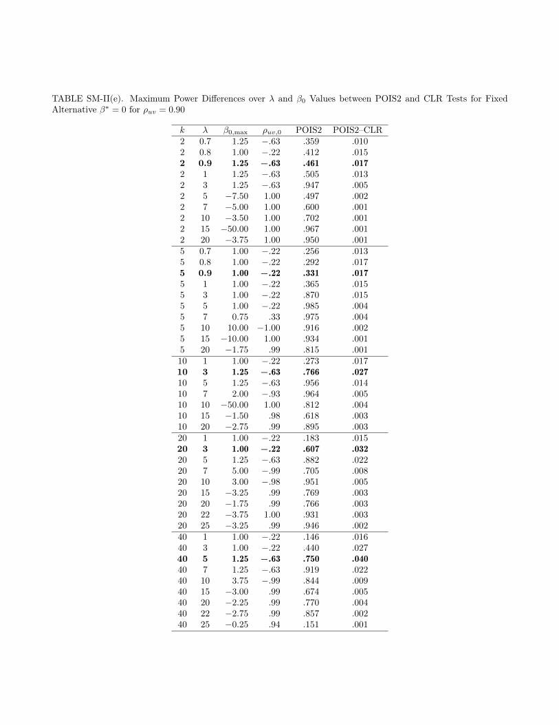
TABLE SM-II(e). Maximum Power Differences over λ and β0 Values between POIS2 and CLR Tests for FixedAlternative β∗ = 0 for ρuv = 0.90

k λ β0,max ρuv,0 POIS2 POIS2–CLR2 0.7 1.25 −.63 .359 .0102 0.8 1.00 −.22 .412 .0152 0.9 1.25 −.63 .461 .0172 1 1.25 −.63 .505 .0132 3 1.25 −.63 .947 .0052 5 −7.50 1.00 .497 .0022 7 −5.00 1.00 .600 .0012 10 −3.50 1.00 .702 .0012 15 −50.00 1.00 .967 .0012 20 −3.75 1.00 .950 .0015 0.7 1.00 −.22 .256 .0135 0.8 1.00 −.22 .292 .0175 0.9 1.00 −.22 .331 .0175 1 1.00 −.22 .365 .0155 3 1.00 −.22 .870 .0155 5 1.00 −.22 .985 .0045 7 0.75 .33 .975 .0045 10 10.00 −1.00 .916 .0025 15 −10.00 1.00 .934 .0015 20 −1.75 .99 .815 .00110 1 1.00 −.22 .273 .01710 3 1.25 −.63 .766 .02710 5 1.25 −.63 .956 .01410 7 2.00 −.93 .964 .00510 10 −50.00 1.00 .812 .00410 15 −1.50 .98 .618 .00310 20 −2.75 .99 .895 .00320 1 1.00 −.22 .183 .01520 3 1.00 −.22 .607 .03220 5 1.25 −.63 .882 .02220 7 5.00 −.99 .705 .00820 10 3.00 −.98 .951 .00520 15 −3.25 .99 .769 .00320 20 −1.75 .99 .766 .00320 22 −3.75 1.00 .931 .00320 25 −3.25 .99 .946 .00240 1 1.00 −.22 .146 .01640 3 1.00 −.22 .440 .02740 5 1.25 −.63 .750 .04040 7 1.25 −.63 .919 .02240 10 3.75 −.99 .844 .00940 15 −3.00 .99 .674 .00540 20 −2.25 .99 .770 .00440 22 −2.75 .99 .857 .00240 25 −0.25 .94 .151 .001

TABLE SM-III. Maximum and Average Power Differences over λ and β0 Values between POIS2 and AR Tests for Fixed Alternative β∗ = 0

(a) Across k patterns for fixed ρuv

POIS2–ARρuv k λmax β0,max ρuv,0 POIS2 max average.0 2 20 0.50 −.45 .49 .079 .012.0 5 20 0.75 −.60 .66 .151 .014.0 10 20 −0.75 .60 .57 .183 .015.0 20 25 0.75 −.60 .57 .217 .016.0 40 25 −0.75 .60 .42 .161 .011.3 2 20 0.50 −.21 .60 .084 .014.3 5 20 −0.75 .74 .56 .163 .020.3 10 20 −1.00 .81 .61 .201 .022.3 20 25 0.50 −.21 .47 .231 .024.3 40 25 −1.00 .81 .47 .194 .019.5 2 20 −0.75 .82 .58 .090 .020.5 5 20 0.50 .00 .66 .182 .031.5 10 20 −1.00 .87 .59 .232 .038.5 20 25 −1.00 .87 .60 .285 .044.5 40 25 −1.25 .90 .54 .248 .040.7 2 20 −0.75 .90 .54 .094 .030.7 5 20 −1.25 .94 .72 .208 .054.7 10 20 −1.25 .94 .67 .281 .069.7 20 25 −1.25 .94 .71 .361 .084.7 40 25 −2.00 .97 .73 .351 .085.9 2 20 −1.00 .97 .64 .105 .033.9 5 20 −1.25 .98 .70 .237 .068.9 10 20 −1.50 .98 .75 .340 .133.9 20 25 −1.25 .98 .76 .455 .160.9 40 25 −1.75 .99 .82 .513 .179

(b) Across ρuv patterns for fixed k

POIS2–ARk ρuv λmax β0,max ρuv,0 POIS2 max average2 .0 20 0.50 −.45 .49 .079 .0122 .3 20 0.50 −.21 .60 .084 .0142 .5 20 −0.75 .82 .58 .090 .0202 .7 20 −0.75 .90 .54 .094 .0302 .9 20 −1.00 .97 .64 .105 .0335 .0 20 0.75 −.60 .66 .151 .0145 .3 20 −0.75 .74 .56 .163 .0205 .5 20 0.50 .00 .66 .182 .0315 .7 20 −1.25 .94 .72 .208 .0545 .9 20 −1.25 .98 .70 .237 .068

10 .0 20 −0.75 .60 .57 .183 .01510 .3 20 −1.00 .81 .61 .201 .02210 .5 20 −1.00 .87 .59 .232 .03810 .7 20 −1.25 .94 .67 .281 .06910 .9 20 −1.50 .98 .75 .340 .13320 .0 25 0.75 −.60 .57 .217 .01620 .3 25 0.50 −.21 .47 .231 .02420 .5 25 −1.00 .87 .60 .285 .04420 .7 25 −1.25 .94 .71 .361 .08420 .9 25 −1.25 .98 .76 .455 .16040 .0 25 −0.75 .60 .42 .161 .01140 .3 25 −1.00 .81 .47 .194 .01940 .5 25 −1.25 .90 .54 .248 .04040 .7 25 −2.00 .97 .73 .351 .08540 .9 25 −1.75 .99 .82 .513 .179

2

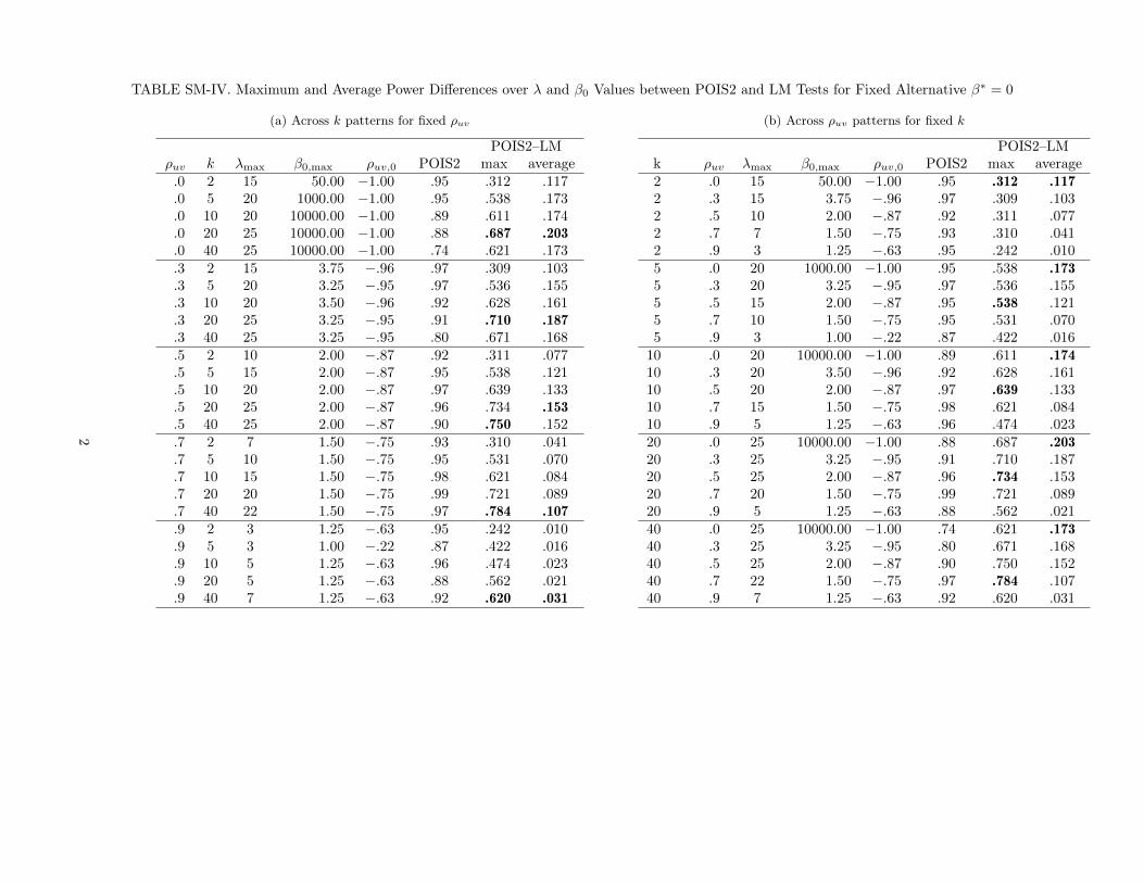
TABLE SM-IV. Maximum and Average Power Differences over λ and β0 Values between POIS2 and LM Tests for Fixed Alternative β∗ = 0

(a) Across k patterns for fixed ρuv

POIS2–LMρuv k λmax β0,max ρuv,0 POIS2 max average.0 2 15 50.00 −1.00 .95 .312 .117.0 5 20 1000.00 −1.00 .95 .538 .173.0 10 20 10000.00 −1.00 .89 .611 .174.0 20 25 10000.00 −1.00 .88 .687 .203.0 40 25 10000.00 −1.00 .74 .621 .173.3 2 15 3.75 −.96 .97 .309 .103.3 5 20 3.25 −.95 .97 .536 .155.3 10 20 3.50 −.96 .92 .628 .161.3 20 25 3.25 −.95 .91 .710 .187.3 40 25 3.25 −.95 .80 .671 .168.5 2 10 2.00 −.87 .92 .311 .077.5 5 15 2.00 −.87 .95 .538 .121.5 10 20 2.00 −.87 .97 .639 .133.5 20 25 2.00 −.87 .96 .734 .153.5 40 25 2.00 −.87 .90 .750 .152.7 2 7 1.50 −.75 .93 .310 .041.7 5 10 1.50 −.75 .95 .531 .070.7 10 15 1.50 −.75 .98 .621 .084.7 20 20 1.50 −.75 .99 .721 .089.7 40 22 1.50 −.75 .97 .784 .107.9 2 3 1.25 −.63 .95 .242 .010.9 5 3 1.00 −.22 .87 .422 .016.9 10 5 1.25 −.63 .96 .474 .023.9 20 5 1.25 −.63 .88 .562 .021.9 40 7 1.25 −.63 .92 .620 .031

(b) Across ρuv patterns for fixed k

POIS2–LMk ρuv λmax β0,max ρuv,0 POIS2 max average2 .0 15 50.00 −1.00 .95 .312 .1172 .3 15 3.75 −.96 .97 .309 .1032 .5 10 2.00 −.87 .92 .311 .0772 .7 7 1.50 −.75 .93 .310 .0412 .9 3 1.25 −.63 .95 .242 .0105 .0 20 1000.00 −1.00 .95 .538 .1735 .3 20 3.25 −.95 .97 .536 .1555 .5 15 2.00 −.87 .95 .538 .1215 .7 10 1.50 −.75 .95 .531 .0705 .9 3 1.00 −.22 .87 .422 .016

10 .0 20 10000.00 −1.00 .89 .611 .17410 .3 20 3.50 −.96 .92 .628 .16110 .5 20 2.00 −.87 .97 .639 .13310 .7 15 1.50 −.75 .98 .621 .08410 .9 5 1.25 −.63 .96 .474 .02320 .0 25 10000.00 −1.00 .88 .687 .20320 .3 25 3.25 −.95 .91 .710 .18720 .5 25 2.00 −.87 .96 .734 .15320 .7 20 1.50 −.75 .99 .721 .08920 .9 5 1.25 −.63 .88 .562 .02140 .0 25 10000.00 −1.00 .74 .621 .17340 .3 25 3.25 −.95 .80 .671 .16840 .5 25 2.00 −.87 .90 .750 .15240 .7 22 1.50 −.75 .97 .784 .10740 .9 7 1.25 −.63 .92 .620 .031

2

TABLE SM-V(a). Average (over λ) Power Differences for λ ∈ 2.5, 5.0, ..., 90.0 between the WAP2 and CLR Testsfor k = 2

β0ρuv,0 WAP2 WAP2–CLR

ρuv = 0 .9 ρuv = 0 .3 .5 .7 .9 ρuv = 0 .3 .5 .7 .9−10000.00 1.00 1.00 .946 .950 .951 .955 .958 .003 .002 .001 .001 .001−1000.00 1.00 1.00 .946 .950 .951 .955 .958 .003 .002 .001 .001 .001−100.00 1.00 1.00 .946 .949 .951 .954 .957 .003 .002 .001 .000 .001−50.00 1.00 1.00 .946 .949 .950 .953 .956 .003 .002 .001 .001 .001−10.00 1.00 1.00 .946 .945 .945 .947 .948 .003 .002 .001 .000 .001−7.50 .99 1.00 .945 .944 .943 .944 .945 .003 .002 .001 .000 .000−5.00 .98 1.00 .944 .941 .938 .938 .937 .003 .001 .001 .001 .000−4.00 .97 1.00 .943 .938 .935 .933 .931 .003 .001 .001 .001 .000−3.75 .97 1.00 .942 .937 .933 .931 .929 .003 .001 .001 .001 .001−3.50 .96 1.00 .941 .936 .932 .929 .927 .002 .001 .001 .001 .001−3.25 .96 .99 .940 .934 .930 .926 .923 .002 .001 .001 .001 .001−3.00 .95 .99 .940 .933 .927 .923 .920 .003 .001 .001 .001 .000−2.75 .94 .99 .938 .930 .925 .920 .916 .003 .001 .001 .000 .000−2.50 .93 .99 .937 .928 .922 .916 .911 .002 .001 .001 .001 .000−2.25 .91 .99 .935 .925 .918 .910 .904 .002 .001 .001 .001 .000−2.00 .89 .99 .932 .920 .912 .904 .896 .002 .002 .001 .001 .001−1.75 .87 .99 .928 .914 .904 .895 .885 .002 .001 .001 .001 .000−1.50 .83 .98 .921 .905 .893 .881 .870 .001 .001 .001 .001 .000−1.25 .78 .98 .910 .890 .876 .861 .847 .001 .002 .001 .001 .001−1.00 .71 .97 .895 .866 .845 .827 .809 .002 .002 .001 .001 .001−0.75 .60 .97 .851 .814 .788 .762 .738 .001 .002 .002 .001 .001−0.50 .45 .95 .736 .681 .646 .613 .584 .002 .002 .002 .002 .001−0.25 .24 .94 .366 .329 .310 .293 .279 .002 .002 .002 .001 .001

0.25 −.24 .83 .366 .410 .447 .488 .544 .001 .001 .002 .002 .0010.50 −.45 .68 .737 .804 .848 .892 .937 .002 .002 .001 .001 .0000.75 −.60 .33 .851 .899 .928 .959 .989 .002 .001 .001 .001 .0001.00 −.71 −.22 .892 .928 .951 .975 .997 .001 .001 .001 .001 .0001.25 −.78 −.63 .911 .942 .959 .979 .997 .001 .002 .001 .001 .0001.50 −.83 −.81 .921 .948 .963 .980 .995 .001 .002 .002 .001 .0001.75 −.87 −.89 .928 .950 .965 .979 .993 .002 .002 .002 .002 .0002.00 −.89 −.93 .932 .953 .965 .978 .991 .001 .002 .002 .002 .0002.25 −.91 −.95 .935 .953 .965 .976 .989 .002 .002 .002 .001 .0002.50 −.93 −.96 .937 .954 .964 .975 .986 .002 .003 .002 .001 .0002.75 −.94 −.97 .938 .955 .964 .973 .985 .003 .003 .002 .001 .0003.00 −.95 −.98 .939 .955 .963 .973 .983 .002 .003 .002 .001 .0003.25 −.96 −.98 .940 .954 .963 .972 .982 .003 .003 .002 .001 .0003.50 −.96 −.99 .941 .954 .962 .970 .980 .003 .003 .002 .000 .0003.75 −.97 −.99 .942 .955 .962 .970 .979 .003 .003 .002 .001 .0004.00 −.97 −.99 .942 .954 .962 .969 .978 .003 .002 .002 .001 .0005.00 −.98 −.99 .944 .954 .960 .967 .974 .003 .002 .002 .001 .0007.50 −.99 −1.00 .945 .953 .957 .964 .970 .003 .002 .001 .001 .000

10.00 −1.00 −1.00 .946 .952 .956 .961 .967 .004 .002 .002 .001 .00050.00 −1.00 −1.00 .946 .950 .952 .956 .960 .003 .002 .001 .000 .001

100.00 −1.00 −1.00 .946 .950 .952 .955 .959 .003 .002 .002 .001 .0011000.00 −1.00 −1.00 .946 .950 .951 .955 .958 .003 .002 .001 .001 .001

10000.00 −1.00 −1.00 .946 .950 .951 .955 .958 .003 .002 .001 .001 .001

TABLE SM-V(b). Average (over λ) Power Differences for λ ∈ 2.5, 5.0, ..., 90.0 between the WAP2 and CLR Testsfor k = 5

β0ρuv,0 WAP2 WAP2–CLR

ρuv = 0 .9 ρuv = 0 .3 .5 .7 .9 ρuv = 0 .3 .5 .7 .9−10000.00 1.00 1.00 .923 .924 .929 .939 .953 .005 .002 .001 .001 .000−1000.00 1.00 1.00 .923 .924 .929 .939 .953 .005 .002 .001 .001 .000−100.00 1.00 1.00 .923 .923 .929 .939 .952 .005 .002 .001 .001 .000−50.00 1.00 1.00 .923 .923 .929 .938 .951 .005 .003 .001 .001 .000−10.00 1.00 1.00 .922 .920 .924 .931 .942 .005 .002 .001 .000 .000−7.50 .99 1.00 .921 .918 .922 .929 .938 .004 .002 .000 .000 .000−5.00 .98 1.00 .919 .915 .917 .923 .931 .004 .001 .000 .000 .000−4.00 .97 1.00 .918 .912 .913 .917 .924 .003 .001 .000 -.000 .000−3.75 .97 1.00 .917 .911 .911 .915 .922 .003 .002 .000 -.000 -.000−3.50 .96 1.00 .917 .910 .910 .913 .920 .003 .001 -.000 -.000 .000−3.25 .96 .99 .916 .909 .908 .910 .917 .003 .001 .000 .000 -.000−3.00 .95 .99 .916 .907 .906 .907 .914 .003 .001 .000 .000 -.000−2.75 .94 .99 .914 .905 .903 .904 .910 .002 .001 .000 .000 -.000−2.50 .93 .99 .913 .902 .899 .900 .904 .002 .001 .001 -.000 .000−2.25 .91 .99 .910 .898 .895 .894 .897 .002 .000 .001 -.000 -.000−2.00 .89 .99 .907 .893 .888 .887 .888 .002 .001 .000 .001 -.000−1.75 .87 .99 .903 .886 .880 .877 .877 .001 .001 .001 .000 .000−1.50 .83 .98 .896 .877 .868 .863 .863 .001 .001 .001 .000 .000−1.25 .78 .98 .885 .861 .850 .842 .839 .002 .001 .001 .000 .000−1.00 .71 .97 .865 .836 .820 .808 .800 .001 .000 -.000 -.000 -.000−0.75 .60 .97 .823 .783 .760 .741 .727 .000 -.000 .001 -.000 -.000−0.50 .45 .95 .705 .649 .618 .592 .572 -.000 -.000 -.001 -.001 -.000−0.25 .24 .94 .340 .311 .294 .282 .272 -.001 -.001 -.001 -.000 -.000

0.25 −.24 .83 .347 .390 .428 .476 .536 -.000 -.001 -.001 -.000 -.0010.50 −.45 .68 .711 .777 .825 .877 .931 .001 .000 .000 .000 .0000.75 −.60 .33 .827 .873 .908 .944 .985 .000 .001 .001 .001 .0001.00 −.71 −.22 .868 .904 .930 .960 .994 .002 .001 .001 .001 .0001.25 −.78 −.63 .887 .915 .940 .966 .994 .001 .001 .004 .003 .0011.50 −.83 −.81 .897 .922 .943 .966 .992 .001 .002 .003 .003 .0011.75 −.87 −.89 .904 .926 .945 .965 .989 .002 .003 .004 .003 -.0002.00 −.89 −.93 .907 .928 .945 .963 .986 .002 .003 .004 .002 .0002.25 −.91 −.95 .910 .930 .945 .961 .984 .001 .004 .004 .001 .0002.50 −.93 −.96 .912 .931 .945 .960 .981 .001 .005 .004 .001 -.0002.75 −.94 −.97 .914 .931 .944 .958 .979 .003 .005 .004 .001 .0003.00 −.95 −.98 .915 .931 .943 .957 .977 .003 .005 .003 .001 .0003.25 −.96 −.98 .916 .931 .942 .956 .976 .003 .004 .003 .001 .0003.50 −.96 −.99 .917 .931 .942 .955 .974 .003 .005 .003 .001 -.0003.75 −.97 −.99 .918 .931 .941 .954 .973 .003 .004 .002 .001 .0004.00 −.97 −.99 .919 .931 .940 .954 .972 .004 .005 .002 .001 .0005.00 −.98 −.99 .920 .930 .939 .951 .968 .004 .005 .002 .000 .0007.50 −.99 −1.00 .922 .929 .936 .948 .963 .005 .004 .001 .001 .000

10.00 −1.00 −1.00 .922 .928 .935 .946 .960 .005 .003 .001 .001 .00050.00 −1.00 −1.00 .923 .925 .930 .941 .955 .005 .003 .001 .000 -.000

100.00 −1.00 −1.00 .923 .924 .930 .940 .954 .005 .003 .001 .000 .0001000.00 −1.00 −1.00 .923 .924 .929 .939 .953 .005 .002 .001 .001 .000

10000.00 −1.00 −1.00 .923 .924 .929 .939 .953 .005 .002 .001 .001 .000

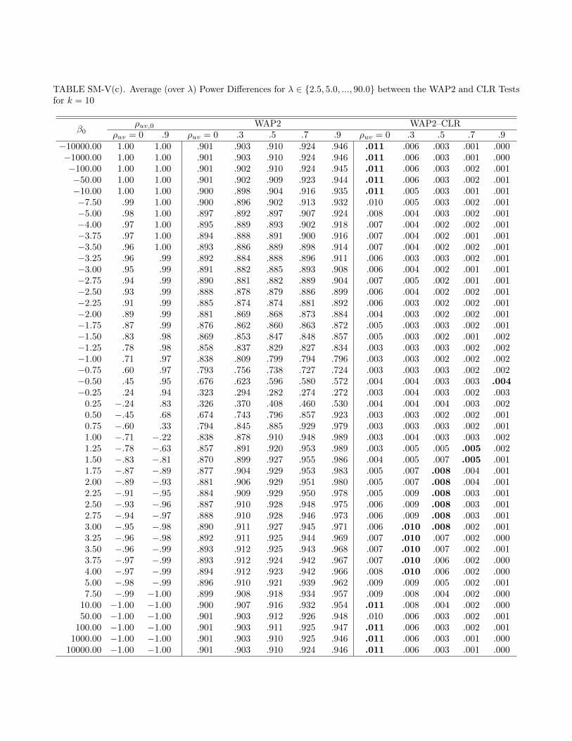
TABLE SM-V(c). Average (over λ) Power Differences for λ ∈ 2.5, 5.0, ..., 90.0 between the WAP2 and CLR Testsfor k = 10

β0ρuv,0 WAP2 WAP2–CLR

ρuv = 0 .9 ρuv = 0 .3 .5 .7 .9 ρuv = 0 .3 .5 .7 .9−10000.00 1.00 1.00 .901 .903 .910 .924 .946 .011 .006 .003 .001 .000−1000.00 1.00 1.00 .901 .903 .910 .924 .946 .011 .006 .003 .001 .000−100.00 1.00 1.00 .901 .902 .910 .924 .945 .011 .006 .003 .002 .001−50.00 1.00 1.00 .901 .902 .909 .923 .944 .011 .006 .003 .002 .001−10.00 1.00 1.00 .900 .898 .904 .916 .935 .011 .005 .003 .001 .001−7.50 .99 1.00 .900 .896 .902 .913 .932 .010 .005 .003 .002 .001−5.00 .98 1.00 .897 .892 .897 .907 .924 .008 .004 .003 .002 .001−4.00 .97 1.00 .895 .889 .893 .902 .918 .007 .004 .002 .002 .001−3.75 .97 1.00 .894 .888 .891 .900 .916 .007 .004 .002 .001 .001−3.50 .96 1.00 .893 .886 .889 .898 .914 .007 .004 .002 .002 .001−3.25 .96 .99 .892 .884 .888 .896 .911 .006 .003 .003 .002 .001−3.00 .95 .99 .891 .882 .885 .893 .908 .006 .004 .002 .001 .001−2.75 .94 .99 .890 .881 .882 .889 .904 .007 .005 .002 .001 .001−2.50 .93 .99 .888 .878 .879 .886 .899 .006 .004 .002 .002 .001−2.25 .91 .99 .885 .874 .874 .881 .892 .006 .003 .002 .002 .001−2.00 .89 .99 .881 .869 .868 .873 .884 .004 .003 .002 .002 .001−1.75 .87 .99 .876 .862 .860 .863 .872 .005 .003 .003 .002 .001−1.50 .83 .98 .869 .853 .847 .848 .857 .005 .003 .002 .001 .002−1.25 .78 .98 .858 .837 .829 .827 .834 .003 .003 .003 .002 .002−1.00 .71 .97 .838 .809 .799 .794 .796 .003 .003 .002 .002 .002−0.75 .60 .97 .793 .756 .738 .727 .724 .003 .003 .003 .002 .002−0.50 .45 .95 .676 .623 .596 .580 .572 .004 .004 .003 .003 .004−0.25 .24 .94 .323 .294 .282 .274 .272 .003 .004 .003 .002 .003

0.25 −.24 .83 .326 .370 .408 .460 .530 .004 .004 .004 .003 .0020.50 −.45 .68 .674 .743 .796 .857 .923 .003 .003 .002 .002 .0010.75 −.60 .33 .794 .845 .885 .929 .979 .003 .003 .003 .002 .0011.00 −.71 −.22 .838 .878 .910 .948 .989 .003 .004 .003 .003 .0021.25 −.78 −.63 .857 .891 .920 .953 .989 .003 .005 .005 .005 .0021.50 −.83 −.81 .870 .899 .927 .955 .986 .004 .005 .007 .005 .0011.75 −.87 −.89 .877 .904 .929 .953 .983 .005 .007 .008 .004 .0012.00 −.89 −.93 .881 .906 .929 .951 .980 .005 .007 .008 .004 .0012.25 −.91 −.95 .884 .909 .929 .950 .978 .005 .009 .008 .003 .0012.50 −.93 −.96 .887 .910 .928 .948 .975 .006 .009 .008 .003 .0012.75 −.94 −.97 .888 .910 .928 .946 .973 .006 .009 .008 .003 .0013.00 −.95 −.98 .890 .911 .927 .945 .971 .006 .010 .008 .002 .0013.25 −.96 −.98 .892 .911 .925 .944 .969 .007 .010 .007 .002 .0003.50 −.96 −.99 .893 .912 .925 .943 .968 .007 .010 .007 .002 .0013.75 −.97 −.99 .893 .912 .924 .942 .967 .007 .010 .006 .002 .0004.00 −.97 −.99 .894 .912 .923 .942 .966 .008 .010 .006 .002 .0005.00 −.98 −.99 .896 .910 .921 .939 .962 .009 .009 .005 .002 .0017.50 −.99 −1.00 .899 .908 .918 .934 .957 .009 .008 .004 .002 .000

10.00 −1.00 −1.00 .900 .907 .916 .932 .954 .011 .008 .004 .002 .00050.00 −1.00 −1.00 .901 .903 .912 .926 .948 .010 .006 .003 .002 .001

100.00 −1.00 −1.00 .901 .903 .911 .925 .947 .011 .006 .003 .002 .0011000.00 −1.00 −1.00 .901 .903 .910 .925 .946 .011 .006 .003 .001 .000

10000.00 −1.00 −1.00 .901 .903 .910 .924 .946 .011 .006 .003 .001 .000

TABLE SM-V(d). Average (over λ) Power Differences for λ ∈ 2.5, 5.0, ..., 90.0 between the WAP2 and CLR Testsfor k = 20

β0ρuv,0 WAP2 WAP2–CLR

ρuv = 0 .9 ρuv = 0 .3 .5 .7 .9 ρuv = 0 .3 .5 .7 .9−10000.00 1.00 1.00 .862 .865 .878 .901 .934 .013 .008 .004 .001 .000−1000.00 1.00 1.00 .862 .865 .878 .900 .934 .013 .008 .004 .001 .000−100.00 1.00 1.00 .862 .864 .877 .900 .933 .013 .007 .003 .002 .000−50.00 1.00 1.00 .862 .864 .876 .899 .932 .013 .007 .003 .002 .000−10.00 1.00 1.00 .860 .860 .870 .892 .923 .012 .007 .002 .002 .001−7.50 .99 1.00 .859 .858 .867 .889 .919 .012 .007 .002 .002 .000−5.00 .98 1.00 .856 .853 .862 .881 .911 .010 .006 .003 .001 .000−4.00 .97 1.00 .854 .849 .858 .876 .905 .009 .005 .003 .002 .000−3.75 .97 1.00 .853 .847 .856 .875 .902 .009 .005 .003 .003 -.000−3.50 .96 1.00 .852 .845 .854 .872 .900 .009 .004 .003 .003 .000−3.25 .96 .99 .851 .843 .852 .869 .897 .009 .004 .003 .002 -.000−3.00 .95 .99 .849 .841 .849 .866 .893 .008 .004 .003 .002 .000−2.75 .94 .99 .847 .839 .846 .862 .889 .008 .005 .003 .001 -.000−2.50 .93 .99 .845 .836 .842 .857 .884 .007 .004 .003 .002 .000−2.25 .91 .99 .842 .832 .837 .851 .877 .006 .004 .002 .002 .000−2.00 .89 .99 .838 .826 .830 .843 .869 .006 .004 .003 .002 .000−1.75 .87 .99 .833 .818 .820 .832 .857 .005 .004 .003 .002 .000−1.50 .83 .98 .825 .807 .806 .817 .841 .005 .005 .003 .002 .000−1.25 .78 .98 .811 .789 .787 .794 .816 .005 .004 .004 .002 .001−1.00 .71 .97 .787 .760 .752 .757 .776 .004 .004 .003 .001 .001−0.75 .60 .97 .739 .701 .688 .688 .704 .004 .002 .002 .001 .000−0.50 .45 .95 .615 .567 .549 .543 .556 .002 .002 .001 .001 .001−0.25 .24 .94 .286 .263 .258 .257 .263 .001 .001 .002 .001 .000

0.25 −.24 .83 .286 .328 .367 .428 .512 .002 .003 .001 .001 .0010.50 −.45 .68 .617 .692 .757 .829 .912 .004 .003 .003 .002 .0000.75 −.60 .33 .743 .800 .849 .906 .971 .004 .004 .003 .003 .0011.00 −.71 −.22 .790 .837 .877 .927 .983 .004 .005 .004 .003 .0021.25 −.78 −.63 .812 .853 .889 .936 .983 .004 .005 .005 .007 .0021.50 −.83 −.81 .824 .861 .897 .936 .980 .004 .006 .008 .007 .0011.75 −.87 −.89 .832 .867 .900 .934 .976 .006 .007 .010 .006 .0012.00 −.89 −.93 .838 .870 .900 .931 .972 .006 .009 .010 .004 .0012.25 −.91 −.95 .842 .872 .900 .930 .969 .007 .010 .010 .004 .0012.50 −.93 −.96 .845 .873 .899 .927 .967 .008 .011 .010 .003 .0012.75 −.94 −.97 .848 .874 .897 .925 .965 .008 .011 .009 .002 .0013.00 −.95 −.98 .849 .875 .896 .924 .963 .008 .011 .008 .002 .0013.25 −.96 −.98 .851 .875 .895 .922 .961 .009 .012 .008 .002 .0003.50 −.96 −.99 .852 .875 .894 .921 .960 .009 .012 .007 .002 .0013.75 −.97 −.99 .853 .875 .893 .920 .958 .009 .012 .007 .002 .0014.00 −.97 −.99 .854 .875 .893 .919 .957 .009 .012 .007 .002 .0015.00 −.98 −.99 .857 .874 .890 .916 .954 .010 .012 .006 .002 .0017.50 −.99 −1.00 .859 .872 .887 .911 .948 .012 .010 .005 .002 .001

10.00 −1.00 −1.00 .860 .870 .885 .909 .945 .012 .010 .005 .002 .00150.00 −1.00 −1.00 .862 .866 .879 .902 .936 .013 .008 .004 .002 .001

100.00 −1.00 −1.00 .862 .865 .879 .901 .935 .013 .008 .004 .001 .0001000.00 −1.00 −1.00 .862 .865 .878 .901 .934 .013 .008 .004 .001 .000

10000.00 −1.00 −1.00 .862 .865 .878 .901 .934 .013 .008 .004 .001 .000

TABLE SM-V(e). Average (over λ) Power Differences for λ ∈ 2.5, 5.0, ..., 90.0 between the WAP2 and CLR Testsfor k = 40

β0ρuv,0 WAP2 WAP2–CLR

ρuv = 0 .9 ρuv = 0 .3 .5 .7 .9 ρuv = 0 .3 .5 .7 .9−10000.00 1.00 1.00 .817 .819 .835 .869 .919 .024 .013 .006 .004 .001−1000.00 1.00 1.00 .817 .819 .835 .869 .919 .023 .013 .006 .004 .001−100.00 1.00 1.00 .817 .818 .834 .867 .917 .023 .013 .006 .004 .001−50.00 1.00 1.00 .817 .817 .833 .867 .916 .023 .012 .005 .004 .001−10.00 1.00 1.00 .814 .810 .826 .858 .905 .022 .010 .005 .003 .000−7.50 .99 1.00 .812 .807 .823 .853 .901 .020 .010 .005 .003 .001−5.00 .98 1.00 .808 .802 .816 .845 .892 .018 .009 .005 .003 .000−4.00 .97 1.00 .804 .797 .810 .838 .884 .016 .008 .004 .003 .000−3.75 .97 1.00 .802 .796 .808 .836 .882 .015 .008 .004 .004 .000−3.50 .96 1.00 .801 .794 .806 .834 .879 .014 .008 .004 .003 -.000−3.25 .96 .99 .799 .792 .803 .831 .876 .013 .008 .004 .003 .000−3.00 .95 .99 .797 .790 .800 .828 .872 .012 .008 .004 .004 .000−2.75 .94 .99 .795 .786 .796 .823 .867 .012 .007 .004 .003 .001−2.50 .93 .99 .792 .783 .792 .817 .861 .011 .007 .005 .002 .001−2.25 .91 .99 .788 .777 .786 .811 .854 .011 .006 .004 .003 .000−2.00 .89 .99 .783 .772 .778 .802 .846 .009 .007 .005 .004 .001−1.75 .87 .99 .777 .761 .767 .790 .833 .009 .006 .004 .003 -.000−1.50 .83 .98 .768 .749 .754 .773 .816 .008 .006 .004 .003 .001−1.25 .78 .98 .752 .730 .730 .750 .791 .007 .006 .004 .003 .000−1.00 .71 .97 .727 .698 .694 .709 .751 .007 .007 .004 .003 -.000−0.75 .60 .97 .672 .633 .624 .632 .675 .006 .005 .004 .001 -.000−0.50 .45 .95 .536 .490 .480 .489 .524 .004 .004 .002 .001 -.002−0.25 .24 .94 .233 .217 .215 .221 .242 .001 .001 -.000 -.001 -.002

0.25 −.24 .83 .237 .275 .318 .383 .491 .001 .000 .000 -.002 -.0020.50 −.45 .68 .539 .621 .697 .788 .892 .004 .004 .004 .003 .0010.75 −.60 .33 .672 .741 .804 .876 .958 .004 .005 .005 .004 .0011.00 −.71 −.22 .727 .784 .837 .901 .974 .005 .006 .006 .006 .0031.25 −.78 −.63 .754 .803 .853 .911 .974 .006 .008 .010 .009 .0041.50 −.83 −.81 .769 .815 .861 .913 .969 .007 .012 .014 .011 .0021.75 −.87 −.89 .779 .824 .865 .910 .965 .008 .016 .016 .008 .0012.00 −.89 −.93 .785 .828 .866 .905 .961 .009 .017 .016 .006 .0012.25 −.91 −.95 .790 .831 .866 .903 .958 .010 .019 .017 .006 .0012.50 −.93 −.96 .794 .833 .864 .901 .955 .011 .020 .016 .005 .0012.75 −.94 −.97 .797 .834 .862 .898 .953 .012 .020 .015 .004 .0013.00 −.95 −.98 .799 .834 .861 .896 .950 .013 .021 .014 .004 .0013.25 −.96 −.98 .801 .834 .859 .894 .949 .014 .021 .013 .004 .0013.50 −.96 −.99 .803 .835 .858 .893 .947 .015 .021 .013 .004 .0013.75 −.97 −.99 .805 .834 .857 .892 .946 .016 .021 .013 .004 .0014.00 −.97 −.99 .806 .834 .855 .890 .944 .016 .021 .012 .004 .0015.00 −.98 −.99 .810 .831 .852 .887 .940 .018 .019 .011 .004 .0017.50 −.99 −1.00 .814 .828 .847 .881 .933 .021 .017 .009 .004 .001

10.00 −1.00 −1.00 .815 .826 .844 .878 .929 .022 .016 .009 .004 .00250.00 −1.00 −1.00 .817 .820 .837 .871 .921 .023 .014 .007 .004 .001

100.00 −1.00 −1.00 .817 .820 .836 .870 .920 .023 .014 .007 .005 .0011000.00 −1.00 −1.00 .817 .819 .836 .869 .919 .024 .013 .006 .004 .001

10000.00 −1.00 −1.00 .817 .819 .835 .869 .919 .024 .013 .006 .004 .001

FIGURE SM-I(a). Power of the significance level .05 CLR, LM, and AR tests and the POIS2 power envelope forfixed null value β0 = 0, varying true value β∗, k = 2, ρΩ = 0, and λ = 5, 20

-6 -4 -2 0 2 4 6-$

p6

0

0.1

0.2

0.3

0.4

0.5

0.6

0.7

0.8

0.9

1

pow

erPOIS2CLRARLM

(i) λ = 5

-6 -4 -2 0 2 4 6-$

p6

0

0.1

0.2

0.3

0.4

0.5

0.6

0.7

0.8

0.9

1

pow

er

POIS2CLRARLM

(ii) λ = 20

FIGURE SM-I(b). Power of the significance level .05 CLR, LM, and AR tests and the POIS2 power envelope forfixed null value β0 = 0, varying true value β∗, k = 5, ρΩ = 0, and λ = 5, 20

-6 -4 -2 0 2 4 6-$

p6

0

0.1

0.2

0.3

0.4

0.5

0.6

0.7

0.8

0.9

1

pow

er

POIS2CLRARLM

(i) λ = 5

-6 -4 -2 0 2 4 6-$

p6

0

0.1

0.2

0.3

0.4

0.5

0.6

0.7

0.8

0.9

1

pow

er

POIS2CLRARLM

(ii) λ = 20

FIGURE SM-I(c). Power of the significance level .05 CLR, LM, and AR tests and the POIS2 power envelope forfixed null value β0 = 0, varying true value β∗, k = 10, ρΩ = 0, and λ = 5, 20

-6 -4 -2 0 2 4 6-$

p6

0

0.1

0.2

0.3

0.4

0.5

0.6

0.7

0.8

0.9

1

pow

er

POIS2CLRARLM

(i) λ = 5

-6 -4 -2 0 2 4 6-$

p6

0

0.1

0.2

0.3

0.4

0.5

0.6

0.7

0.8

0.9

1

pow

er

POIS2CLRARLM

(ii) λ = 20