�

��

L. T. Biegler Carnegie Mellon University

January, 2012

A Nonlinear Programming Path to NMPC and Real-Time

Optimization

Overview

•� Process Optimization – Why and How?

•� Two Key Concepts –� Newton Barrier NLP

–� NLP Sensitivity

•� LDPE Case Study –� Parameter Estimation

–� NMPC � asNMPC

–� MHE � asMHE

–� RTO � D-RTO

•� Where to NMPC and NLP?

•� Conclusions

Why Process Optimization?

•� Parameter Estimation and Model Discrimination •� Equipment and Flowsheet Design •� Process Operations, Transients and Upsets

•� Better Results than with “Experience” •� Consistent Results among all Practitioners •� Support and Enhance Process Understanding •� Reduce Cycle Time by Orders of Magnitude

Case Study

Improvement�

(D)AE Model

C(z, z , u, p, t) = 0�

p u(t)�

Optimization

Min f(x)�s.t. x � X�

(D)AE Model

C(x) = 0�x={z, z , u, p, t}�

How Process Optimization?

Optimization Formulations and Models

Closed

Open

Variables/Constraints

102 104 106

Black Box

Finite Differences

Full First Derivatives

First and Second Derivatives

100

Compute Efficiency

SQP

rSQP

NLP Barrier

DFO

Barrier Methods for Large-Scale

Nonlinear Programming

0

0)(s.t

)(min

�

=

��

x

xc

xfnx

Original Formulation

0)(s.t

ln)()( min1

=

�= �=

��

xc

xxfxn

i

ix n

μ�μBarrier Approach

Can generalize for

��As μ � 0, x*(μ) � x* Fiacco and McCormick (1968)

a � x � b

Barrier Problem Solution

�� Newton Directions (KKT System)

0 )(

0

0 )()(

=

=�

=�+�

xc

eXv

vxAxf

μ

�

�� Solve

���

�

�

�

�

�+�

�=

���

�

�

�

���

�

�

� �

eXv

c

vAf

d

d

d

XV

A

IAW x

T

0

00

μ

�

�

�

�� Reducing the System

xv VdXveXd 11 ����= μ

��

��

���=�

�

��

���

��

� �++ c

d

A

AW x

T

μ

�

0VX 1�

=�

IPOPT Code – www.coin-or.org

),,x(LW),x(cA

)x(diagX...],,,[e

xx

T

���=�=

==

1 1 1

IPOPT Features (Wächter, Laird, B., 2002-2009)

Newton-Based Barrier Method

•� Globally, superlinearly convergent (Wächter and B., 2005)

•� Easily tailored to different problem structures

Line Search Globalization

•� l2 exact penalty merit function •� augmented Lagrangian merit

function •� Filter method (extended from

Fletcher and Leyffer)

Hessian Calculation

- BFGS (full/LM and reduced space) - SR1 (full/LM and reduced space) - Exact full Hessian (direct)

- Exact reduced Hessian (direct) - Preconditioned CG

Widely Available

•� Eclipse License and COIN-OR

distribution: http://www.coin-or.org

•� Solved on many thousands of test problems and applications

•� Broad, growing user community

NLP Sensitivity

Parametric Program

NLP Sensitivity � Rely upon Existence and Differentiability of Path

� Main Idea: Obtain and find by Taylor Series Expansion

Optimality Conditions

Solution Triplet

NLP Sensitivity with IPOPT (Pirnay, Lopez Negrete, B., 2011)

Optimality Conditions of

Obtaining

� Already Factored at Solution

� Sensitivity Calculation from Single Backsolve

� Approximate Solution Retains Active Set

KKT Matrix IPOPT

Apply Implicit Function Theorem to around

NLP Sensitivity

Optimum change with parameters p?

•� Identify sensitive parameters

•� What is sensitivity of the optimum to disturbances and model mismatch?

•� Information obtained essentially free (one backsolve for each perturbation)

•� Starting point for parametric optimization problems

13

NLP Sensitivity

Response Surface for Degrees of Freedom

•� Reduced Hessian extraction from IPOPT

–� Not directly generated by solver, but easily extracted from KKT conditions

•� Split x into degrees of freedom (d) and basic (b) variables

•� Linearized KKT Conditions are:

•� The solution leads to

11

-� j-th column of reduced Hessian inverse. -� requires single back-solve with KKT matrix already factorized!

Change RHS

Z =�Ab

�1Ad

I

�

�

��

�

�

��

NLP Sensitivity

Parameter and State Estimation

•� Analyze sensitivity of estimates with changes in data

12

•� Introduce perturbations , , and , , ,,,,,,,,, a

principal

axes of V �

99%

95%

90%�*

Approximate Confidence Region �

(� - �*)TV�-1 (� - �*) � �(�)�

tf, final time u, control variables p, time independent parameters

t, time z, differential variables y, algebraic variables

Dynamic Optimization Problem

min � z(t), y(t),u(t), p,t f( )

dz( t)

dt= F z(t), y(t), u( t), t, p( )

G z(t), y(t),u(t),t, p( ) = 0

ul

ul

ul

ul

o

ppp

utuu

ytyy

ztzz

zz

��

��

��

��

=

)(

)(

)(

)0(

s.t.

Dynamic Optimization Approaches

DAE Optimization Problem

Multiple Shooting

Embeds DAE Solvers/Sensitivity Handles instabilities

Single Shooting

Hasdorff (1977), Sullivan (1977), Vassiliadis (1994)� Discretize controls

Simultaneous Collocation (Direct Transcription)

Large/Sparse NLP - Betts; B�

Apply a NLP solver

Efficient for constrained problems

Simultaneous Approach

Larger NLP

Discretize state, control variables

Indirect/Variational

Pontryagin(1962)

Bock and coworkers

Take Full Advantage of Open Structure

•� Many Degrees of Freedom

•� Periodic Boundary Conditions

•� Multi-stage Formulations

�

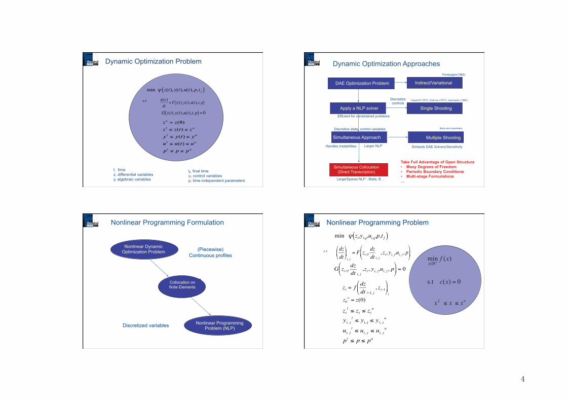
Nonlinear Dynamic Optimization Problem

Collocation on finite Elements

(Piecewise) Continuous profiles

Nonlinear Programming Problem (NLP)

Discretized variables

Nonlinear Programming Formulation Nonlinear Programming Problem

uL

x

xxx

xc

xfn

��

=

��

0)(s.t

)(min

min � zi,yi,q,ui,q,p,t f( )

dz

dt

�

� �

�

� �

i, j

= F zi-1,dz

dt i, j

, zi , yi, j,ui, j , p�

� �

�

� �

G zi-1,dz

dt i, j

,zi , yi, j,ui, j , p�

� �

�

� � = 0

zil� zi � zi

u

yi, jl� y i, j � yi, j

u

ui, jl� ui, j � ui, j

u

pl� p � pu

s.t.

zi = fdz

dt i�1, j

, zi�1

�

� �

�

� �

i

z0

o= z(0)

Off-line Case Studies

•� Dynamic Bioprocess Optimization •� Parameter Estimation of Batch Data •� Synthesis of Reactor Networks •� Crystallization Temperature Profiles •� Optimal Batch Distillation Operation •� Satellite Trajectories in Astronautics •� Batch Process Integration •� Simulated Moving Bed Optimization •� Optimization of Polymerization

Processes •� Optimal Pressure Swing Adsorption

On-line Case Studies •� NMPC of Tenn. Eastman Process •� Source Detection of Water Networks •� Cross-directional Sheet-forming

Processes •� Thermo-mech. Pulping NMPC •� D-RTO for Gas Pipelines •� Air Traffic Conflict Resolution •� NMPC for Refinery Distillation •� Ramping for Air Separation Columns •� Startup for Combined Cycle Power

Generation •� Cyclic Operation for LDPE

Process

Some Case Studies with Simultaneous Collocation

LDPE

Low-Density Polyethylene Process

Flowrate

Reactor

Temperatures

Jacket

Temperatures

Ethylene Inlet Temperatures

Recycle System

and Flash Separation

Low-Pressure Recycle

High-Pressure Recycle

Polymer Melt Index

Initiators Initiators Initiators Initiators

Ethylene Cold-Shots

Chain-Transfer Agent

- Free-Radical Polymerization at Supercritical Conditions (2000 - 3000 atm)

- Multi-Zone Tubular Reactor (2 Km Long Pipe)

- Highly Exothermic, Keep Low Conversions (20-35%)

- High Throughput (300,000 Ton/yr)

-� Multi-Product Operations ( > 20 Grades)

-� Inputs/ Outputs for control and optimization

Large-Scale Parameter Estimation

~ 35 Elementary Reactions ~100 Kinetic Parameters

�� Complex Kinetic Mechanisms

Large-Scale Parameter Estimation

�� Parameter Estimation for Industrial Applications

�� Use Rigorous Model to Match Plant Data Directly

�� Start with Standard Least-Squares Formulation

Rigorous Reactor Model

�� Special Case of Multi-Stage Dynamic Optimization Problem

�� Solve using Simultaneous Collocation-Based Approach

Least-Squares

1 data set 6 data sets

x 6 500 ODEs

1000 AEs

3000 ODEs

6000 AEs

�� Multi-Zone Tubular Reactor – Quasi Steady-State �� Data Sets: Operating Conditions and Properties for Different Grades �� Match: Temperature Profiles and Product Properties

�� On-line Adjusting Parameters �� Track Evolution of Disturbances �� Kinetic Parameters � Development and Discrimination among Rigorous Models

�� Results �� Single Data Set (On-line Adjusting Parameters)

�� Multiple Data Sets (On-line Adjusting Parameters + Kinetics)

Bottleneck - Memory Requirements In KKT Factorization Step

(Handled through blockwise

decomposition of KKT matrix)

Large-Scale Parameter Estimation

Improved Prediction Core Temperature Profile

LDPE Parameter Estimation

Grade A

Grade B

Zone 1 Zone 2 Zone 3 Zone 4

Zone 1 Zone 2 Zone 3 Zone 4

Sensitivity-based Confidence Regions

•�Modify KKT (full space) matrix if nonsingular

� �1 - Correct inertia to guarantee descent direction

� �2 - Deal with rank deficient Ak

•�KKT matrix factored by indefinite symmetric factorization

•�Solution with �1=0 � sufficient second order conditions

•�Parameter Estimation Result – unique parameters

•�Reduced Hessian available to calculate confidence regions

�

�

�

�

+�+

IA

AIWT

k

kkk

2

1

�

�

ue parametersp

aaaaaaaaaaaaaaaaaatte ttettttttttttttttttttttttttttttetttetttettttttttttee ccccccccccoccccccccccccccccccccccccccccccccccccThe image cannot be displayed. Your computer may not have enough memory to open the image, or the image may have been corrupted. Restart your computer, and then open the file again. If the red x still appears, you may have to delete the image and then insert it again.

On-line Issues: Model Predictive Control (NMPC)

Process

NMPC Controller

d : disturbances

z : differential states

y : algebraic states

u : manipulated

variables

ysp : set points

( )

( )dpuyzG

dpuyzFz

,,,,0

,,,,

=

=�

NMPC Estimation and Control

minu

J(x(k)) = �(zl ,ul )+F(zN )l= 0

N

�

s.t.zl +1 = f (zl ,ul ))

z0 = x(k)Bounds

NMPC Subproblem

Why NMPC?

�� Track a profile – evolve from

linear dynamic models (MPC)

�� Severe nonlinear dynamics (e.g,

sign changes in gains)

�� Operate process over wide range

(e.g., startup and shutdown)

Model Updater

( )

( )dpuyzG

dpuyzFz

,,,,0

,,,,

=

=�

MPC - Background Motivate: embed dynamic model in moving horizon framework to drive process to desired state (Rawlings and Mayne, 2009)

Generic MIMO controller Direct handling of input and output constraints Slow process time-scales – consistent with dynamic operating policies

Different types

Linear Models: Step Response (DMC) and State-space Empirical Models: Neural Nets, Volterra Series Hybrid Models: (QP/MIQP�), apply parametric programming and Explicit MPC

First Principle Models – direct link to off-line planning

NMPC Pros and Cons

+ Operate process over wide range (e.g., startup and shutdown) + Vehicle for Dynamic Real-time Optimization - Need Fast NLP Solver for time-critical, on-line optimization - Computational Delay from On-line Optimization degrades performance

�������������� ������������

Optimization and Optimal Control •� Pontryagin (1959), Bryson and Ho (1969), Ray (1981), Sargent

and coworkers (1970s),�

Model Predictive Control •� Evolution from LQ, MPC (Kleinman, 1975; Kwon and Pearson,

1977), •� DMC (Cutler and Ramaker, 1979), QDMC (Garcia and

Morshedi,1984) •� Concepts and Analysis: Allgöwer and coworkers (1989 - ),

Bordons and Camacho (2001), Rawlings and Mayne (2009), Grüne and Pannek (2011)

•� Real-time iteration (Diehl, Li, Ohtsuka, Oliveira, Santos, 1989 - ) •� Neighboring extremal approaches (Bonvin, Marquardt, 2002 - )

What about Fast NMPC?

•� Fast NMPC is not just NMPC with a fast solver (Engell, 2007)

•� Computational delay – between receipt of process measurement and injection of control, determined by cost of dynamic optimization

•� Leads to loss of performance and stability (see Rawlings and Mayne, 2009; Findeisen and Allgöwer, 2004; Santos et al., 2001)

Can computational delay be overcome? -� Fast Newton-based NMPC -� Cheap NLP Sensitivity

��������� ������������������������tk�����tk+1 �

Advanced Step Nonlinear MPC (Zavala, B., 2009)

min J(x(k), u(k)) = F(xk +N |k ) + �(xl |k,vl |k )l= k +1

k +N�1

�

s.t. xk +1|k = f (x(k),u(k))

xl +1|k = f (xl |k,vl |k ), l = k +1,...k + N -1

xl |k � X, vl |k �U, xk +N |k � X f

������������������������������������������������� ��

��������������������������������

��������������� !��������� "���������

��� �

#�� �

�� ��

� #� !$��

���������� ������������������������tk�����tk+1 �

���������������������������%�������������������� ! �

Wk Ak �I

AkT 0 0

Zk 0 Xk

�

�

� � �

�

�x

��

�z

�

�

� � �

�

� � �

=

0

�

xk +1|k � x(k +1)

0

�

�

� � � � �

�

� � � � �

Advanced Step Nonlinear MPC (Zavala, B., 2009)

������������������������������������������������� ��

��������������������������������

#�� � � #�� ! �

��� ! ���� �

��������������� !��������� "��������� �� ��

##

#� !$��

���������� ������������������������tk�����tk+1 �

���������������������������%�������������������� ! �

���������� ! ������������������������tk+1�����tk+2 �

Advanced Step Nonlinear MPC (Zavala, B., 2009)

min J(x(k +1), u(k +1)) = F(xk +N +1|k +1) + �(xl |k +1,vl |k +1)l= k +2

k +N

�

s.t. xk +2|k +1 = f (x(k +1),u(k +1))

xl +1|k +1 = f (xl |k,vl |k ), l = k +2,...k + N

xl |k +1 � X, vl |k +1 � U, xk +N +1|k +1 � X f

������������������������������������������������� ��

��������������������������������

��������������� !��������� "��������� �� ��

#�� � � #�� ! �

��� ! ���� �

#� "$� !�

Offset-free Formulation •� Apply MHE results as state and output corrections for NMPC problem •� Modify with an advanced step approach � as-MHE

Combining MHE & NMPC ����������������������� �

Process

NMPC Controller

d : disturbances

z : differential states

y : algebraic states

u : manipulated

variables

ysp : set points

( )

( )dpuyzG

dpuyzFz

,,,,0

,,,,

=

=�

Model Updater

( )

( )dpuyzG

dpuyzFz

,,,,0

,,,,

=

=�

Advanced-step MHE (Zavala, Lopez Negrete, B. 2009 - 2011)

Measured

outputs

Estimated

states

ktNkt � 1+�Nkt 2+�Nkt

p�

Background: At tk, having xk and uk, approximate xk +1 and yk +1. Solve the

extended MHE problem from k-N to k+1. Let p0 = approximate yk +1.

Iterate: Set k = k+1 and go to background.

On-line update: At tk+1, obtain yk+1. Set p = yk+1 and use NLP sensitivity

to get fast update xk+1.

NLP Sensitivity used for State Approximation and Covariance Updates

Chain-Transfer Agent

NMPC-MHE Scenario

LDPE

Flowrate Ethylene Inlet Temperatures

Low-Pressure Recycle

Hyper-Pressure Recycle

Ethylene Cold-Shots

Initiators Initiators Initiators Initiators

Recycle System and Flash Separation

Measured

Measured

Not Measured

Fouling of reactor wall – treated as (imposed, unmeasured) disturbance

Time (Days)

Heat Transfer Coefficient

Fouling

Defouling

Cannot Remove Heat of Reaction - Drop Production to Avoid Runaway

FoulingMHE+NMPC for LDPE Process

Centralized Control Framework Including PDAE Reactor Model - Ramp Reactor Heat-Transfer Coefficients to Simulate Fouling-Defouling Behavior

- MHE to Infer Heat-Transfer and Model States (e.g. Wall Profile)

- NMPC to Stabilize Temperature Profile

NMPC-MHE Scenario

Time

Heat-Transfer Coefficient

Wall Temperature

Initial Guess

Initial Guess

MHE Performance – Convergence to True State

MHE Recovers from Poor Initial Guesses in Few Time Steps

Distributed Temperature Measurements

Make Reactor Strongly Observable Zavala & B., 2010

Reference Profile

Controller Stabilizes Temperature Levels but Needs to Drop Production as Fouling Advances

NMPC Performance – Tracking Objective

NMPC-MHE Scenario

Core Temperature

Overall Production

Fouling

But� LDPE Reactor has Many Degrees of Freedom -Not Fully Exploited with Conventional NMPC-

Minimize Transition Time

NMPC with Economic Objectives Beyond RTO and MPC Regulation � D-RTO

Plant

DR-PE c(x, u, p) = 0

RTO c(x, u, p) = 0

APC

y

p

u

w

Plant

DR-PE c(x, x , u, p) = 0

D-RTO

c(x, x , u, p) = 0

PC

y

p

u

m

Benefits of combining RTO with NMPC? •�Direct, dynamic production maximization •�Remove artificial setpoint objective •�Remove artificial steady state problem •�Overcomes neglect of dynamic uncertainty •�Leads to significant improvements (up to

10%) over steady state RTO

Challenges with D-RTO Replace regulation objective with economic objective in NMPC?

Bartusiak, Young et al. (2007) Chachuat et al. (2008), Dadhe and Engell (2008), Engell (2007, 2009) Busch, Kadam Marquardt et al. (2008) Odloak, Zanin, Tvrzska de Gouvea (2002) Zanin, Tvrzska de Gouvea Odloak (2000) Diehl, Amrit and Rawlings (2010)

Angeli and Rawlings (2010) Angeli, Amrit and Rawlings (2011)

Robust Stability of Lyapunov function � must be K� function (e.g., strong convexity of stage cost)

Many open Stability/Robustness Questions Still Remain

- does optimum go to a steady state or not? - how do we enforce optimal steady state? - how to consider cyclic problems?

Remedy: Regularize economic objective with KK� function for stage cost?

Min wi�(zi,ui )+Profiti{ }+ wN F(zN )+ProfitN

i

� Min Profit i{ }+ ProfitN i

�

•�Nominal Stability – ensure

For the rotated stage costs (transformed Lagrange function),

If is strongly convex, then the stage cost assumption is satisfied. If not, add regularization terms to rotated stage costs. Allows straightforward extension to ISS stability

Strong convexity property can be checked/corrected off-line - Related to strong duality (Diehl et al., 2011) - Related to dissipativity (Angeli et al., 2011)

Li (z, v )

Li (0, 0) = 0

Economic NMPC Stability Analysis (Huang, Harinath, B., 2011)

e

Time (Days)

Heat Transfer Coefficient

Fouling

Defouling

Persistent Dynamic Disturbances – Strong Effect on Profitability

Cannot Remove Heat of Reaction - Drop Production to Avoid Runaway

Potential Economic Benefits of 1% Production Increase

0.01 x (300,000 Ton/yr) x (1,500 $/Ton) = 4,500,000 $/yr

Dynamic RTO for LDPE Process (Zavala, B., 2010)

3% More Production

D-RTO for LDPE Process NMPC Performance – Regularized Economic Objective

Maximize Production

Reference Profile

Economics-Oriented NMPC Moves Away from Suboptimal Reference Profile

Distributes Production Along Reactor Efficiently e.g. More Production in Less Fouled Zones

Minimize Transition Time

Core Temperature

Overall Production

Economics-Oriented Tracking

Improving NMPC for LDPE Background Computational Performance - NMPC - Full-Discretization + IPOPT (MA57), Quad-Core Pentium IV

- Prediction Horizon 5 Time Steps, NLP ~ 50,000 Constraints, 300 DOF

Sampling Time = 2 min

- Scale-Up With Prediction Horizon and Effect of KKT Matrix Reordering

NLP with 350,000 Constraints and 1,000 DOF Solved in ~ 2 Minutes

High Level NLP Design (Laird, Wächter, 2006 -)

NLP Interface

IPOPT Algorithm

Standard NLP

Linear Algebra Interface

Default Linear Algebra

Large Structured

NLP

Specialized Linear Algebra

Linear KKT structure abstracted from algorithm

Optimization Models, NLP Interfaces

•� AMPL, ASL (Gay et al., 1985) •� Optimica, JModelica (Åkesson, 2008) •� PyOMO (Sandia group, 2010) •� ACADO (Diehl et al., 2010)

Reuse L/U Factors of K with Schur Complement

Background NLP requires more than �T?

Background Optimization

Online Update

NLP Type Stability Properties

Ideal None NLP Various Nom./ISS

Real-time Iteration

None QP Multiple shooting

Nominal

Neighboring Extremal

Only once KKT/QP

Single shooting

Nominal

asNMPC Every step KKT Simultaneous Collocation

Nom./ISS

amsNMPC (Yang, B., 2012)

Every n steps

KKT+ Schur

SimultaneousCollocation

Nominal

Advanced Step Framework - Into the Future

•� Stability Properties for asNMPC (Zavala, B., 2009)

–� Nominal stability – no disturbances nor model mismatch

–� Input to State Stability (ISS) - Assumes RPI set (no path constraints)

–� Guarantee specified level of uncertainty? •� Adapt tube-based approaches for NMPC (Mayne et al., 2011)

•� Constraint relaxations

•� Direct calculation of RPI regions

•� Moving Horizon Estimation (Lopez Negrete, Huang, B., 2010, 2011)

–� Fast sensitivity-based smoothed covariance of arrival cost

–� Robust stability for asMHE?

–� Statistical properties of arrival cost formulations?

•� Extension to economic objectives (Huang, Harinath, B., 2011) –� Nominal and ISS stability based on rotated stage costs

–� Extended to cyclic processes

–� Development of unbiased regularized stage costs?

–� Stability with incorporation of asMHE?

Bigger NLPs are not harder to solve

•� Embrace and exploit size, sparsity and structure •� Exact first and second derivatives are essential •� Newton-based optimization is fast •� Optimal sensitivity is (nearly) free

Chemical Process Operations: RTO � D-RTO •� Essential for Batch Processes, Cyclic Processes, Transient Operations •� Need for First-Principles Dynamic Models •� Extension to On-Line Economic Decision-Making

NMPC and MHE Computational Strategies •� Full-Discretization + Fast Sensitivity Calculations •� Large-scale LDPE process with DAE model

From NMPC Setpoints to Economic Optimization •� Direct optimization in real-time •� Maintain stability and exploit uncertainties •� Still many open questions

For more information: http//:numero.cheme.cmu.edu

http//:capd.cheme.cmu.edu

Conclusions

Many Thanks to: Research Colleagues

–� Prof. Johan Åkesson –� Dr. Juan Arrieta –� Dr. Gilvan Fischer –� Prof. Antonio Flores –� Ajit Gopalakrishnan –� Eranda Harinath –� Dr. Rui Huang –� Prof. Carl Laird –� Dr. Rodrigo Lopez Negrete –� Prof. Andreas Wächter –� Dr. Victor Zavala –� Xue Yang

Lynne W. Biegler

and � To the NPC community In humble thanks for your

award and recognition

For more details�

MOS-SIAM Series on Optimization •�NLP Theory and Algorithms

•�Steady State Process Optimization

•�Dynamic Process Optimization

•�Optimal Control

•�Sequential Approaches

•�Simultaneous Approaches

•�Mathematical Programs with

Complementarity Constraints

For more information: http://www.siam.org/catalog