lable at ScienceDirect

Applied Thermal Engineering 31 (2011) 2439e2448

Contents lists avai

Applied Thermal Engineering

journal homepage: www.elsevier .com/locate/apthermeng

A nonlinear inverse problem in estimating the heat flux of the discin a disc brake system

Yu-Ching Yang, Wen-Lih Chen*

Clean Energy Center, Department of Mechanical Engineering, Kun Shan University, No. 949, Dawan Rd., Yongkang Dist., Tainan City 710, Taiwan ROC

a r t i c l e i n f o

Article history:Received 26 January 2011Accepted 7 April 2011Available online 16 April 2011

Keywords:Inverse problemDisc brakeHeat fluxConjugate gradient method

* Corresponding author. Tel.: þ886 62050496; fax:E-mail address: wlchen@mail.ksu.edu.tw (W.-L. Ch

1359-4311/$ e see front matter � 2011 Elsevier Ltd.doi:10.1016/j.applthermaleng.2011.04.008

a b s t r a c t

In this study, an inverse algorithm based on the conjugate gradient method and the discrepancy principleis applied to estimate the unknown space- and time-dependent heat flux of the disc in a disc brakesystem from the knowledge of temperature measurements taken within the disc. In the direct problem,the specific heat and thermal conductivity are functions of temperature; hence this is a nonlinear inverseproblem. The temperature data obtained from the direct problem are used to simulate the temperaturemeasurements, and the effect of the errors in these measurements upon the precision of the estimatedresults is also considered. Results show that an excellent estimation on the space- and time-dependentheat flux can be obtained for the test cases considered in this study. The current methodology can be alsoapplied to the prediction of heat flux in the pads, and then the heat partition coefficient between the discand the pad in a brake system can be calculated.

� 2011 Elsevier Ltd. All rights reserved.

1. Introduction

In recent decades, disc brakes have increasingly become morepopular and gradually found their ways in many different types ofvehicles, ranging from light motorcycles to heavy road trucks oreven trains. They offer several advantages over drum brakes,including better stopping performance (disc cooled readily), easierto control (not self-applying), less prone to brake fade, and quickerrecovery from immersion, which largely contributed to theirpopularity. However, after long repetitive braking, brake fade couldstill set in and compromise the performance of a disc brake due tothe change of friction characteristics caused by temperature rise andoverheating of brake components. Overheated components couldfurther lead to more problems such as thermal cracks, plasticdeformation, brake fluid vaporization, and premature wear, and thelife span of a disc brake could be shortened as a result. Therefore, toaccurately predict the temperature rise in a disc brake system is ofeminent importance in the early design stage. Yet, owing to theinteractions of several physical phenomena, the prediction of discbrake performance is highly complicated. First, disc braking is a verydynamic and highly transient phenomenon in which extremelylarge temperature gradients can be generated at the vicinity of disc/pad interface in a fraction of a second during a high-g decelerationand result in excessive thermal stresses, a phenomenon termed as

þ886 62050509.en).

All rights reserved.

“thermal shock”. Thermal shock can give rise to surface cracks andplastic deformation on the disc, making disc surfaces uneven. Asa consequence, the heat dissipation area at the discepad interface islargely reduced and becomes non-uniform [1]. Frictional heatingalso produces thermal deformation and elastic contact which, inturn, largely affect the contact pressure and temperature onsliding interface. These phenomena are termed “thermomechanicalcoupling or thermomechanical effects”, and are one of the majorcauses of creating hot spots on the sliding interface. Hot spots couldfurther induce frictional vibration known as “judder”, which affectsdriving comfort and compromises driving safety if inexperienceddrivers react to it improperly [2]. Second, asperities and wearparticles can accumulate and form a thin layer called “third body” atthe discepad interface. The presence of the third body not onlychanges friction properties at the discepad interface but also acts asa thermal resistance to the heat dissipated into the disc. Third, as theapplication of disc brakes has been widened, the geometries ofbrake components are becoming more sophisticated. For example,the use of drilled-through holes and slots on disc is common inmotorcycle’s disc brake systems, and pads made of individualelements have been widely employed on the disc brake systems ofhigh-speed trains. This development toward complex geometrymakes thermal analysis even more difficult.

Since there exists complex coupling of tribological, mechanical,and thermal behaviors in a disc brake, a comprehensive analysis ofits performance is extremely difficult, if not impossible. Then theproblem is generally simplified by decoupling the thermal behaviorfrom others through the introduction of some boundary conditions

Nomenclature

c specific heat (J kg�1 K�1)h convection heat transfer coefficient (Wm�2 K�1)J functionalJ0 gradient of functionalk thermal conductivity (Wm�1 K�1)p direction of descentpmax maximum pressure in the pad (Nm�2)q heat flux density (Wm�2)q0 initial guess of heat flux density (Wm�2)q0 heat flux density at time t¼ 0 (Wm�2)r radial coordinate (m)r1 inner disc radius (m)r2 inner pad radius (m)r3 outer radius of the disc and the pad (m)S frictional surface (m2)T temperature (K)T0 initial temperature (K)TN surrounding temperature (K)t time coordinate (s)tf final time (s)z axial coordinate (m)

z2 half disc thickness (m)

Greek symbolsD small variation qualitya thermal diffusivity (m2 s�1)b step sizeg conjugate coefficientx thermal effusivity (J m�2 K�1 s�0.5)h very small valueq0 pad contact angle (rad)l variable used in adjoint problemm friction coefficientr density (kgm�3)s standard deviations transformed time coordinatef heat partition coefficient6 random variableu0 initial angular velocity of the disc (s�1)

Superscripts/subscriptsK iterative numberd discp pad

Y.-C. Yang, W.-L. Chen / Applied Thermal Engineering 31 (2011) 2439e24482440

at the discepad interface. In thermal analysis, accurate estimationof the total energy absorbed by the brake system and the distri-butions of this energy among the disc and the pads is very crucial.The former can be reasonably assumed to be the same as thereduction of kinetic energy of the vehicle during the brakingprocess, while the determination of the latter is not straightfor-ward. Two interface postulations, perfect contact and imperfectcontact, are commonly adopted to resolve this issue. In the perfectcontact postulation, the surface temperatures between the disc andthe pad at the interface are equal, and with a very short brakingtime, both disc and pad can further be regarded as semi-infinitesolids. Then the ratio between the heat fluxes dissipated into thedisc and pad can be obtained analytically [3,4]. However, as thetime scale of a brake problem is very short, it is highly transient innature. Therefore thermal equilibrium at the interface, a staterequired for equal surface temperature to exist, cannot be main-tained at each moment. In the imperfect postulation, on the otherhand, the third body is present between the disc and the pad at thediscepad interface. It acts as a thermal contact resistance, and thefriction heat is assumed generated at the pad surface and thendissipated into the disc through the third body. As a consequence,the surface temperatures of the disc and pad are not equal, whichcomplies with some experimental observations of the clear pres-ence of temperature gradients between pad and disc surfaces. Yetin this practice, difficulty arises to accurately determine the value ofthe thermal resistance of the third body. It requires some experi-ments specifically designed to measure thermal resistance undervarious braking conditions [5]. Furthermore, there have beenarguments on the deficiencies of this approach, mainly the over-look of thermal interface inertia and the assumption of a lineartemperature gradient across the third body [6]. From the briefreview above, it is clear that a more precise friction model forthe disc/pad interface is yet to be formulated; and due to thecomplexity of the problem, developing such amodel will be heavilyrelied on the calibrations with experimental data, especially toestablish the relationship among the heat dissipated into the discand the mechanical, tribological, and thermal parameters involvedin a disc brake process.

The studies of inverse heat conduction problem (IHCP) in recentyears have offered convenient alternatives to experimental mea-surements to obtain accurate thermo-physical quantities such asheat sources, material’s thermal properties, and boundarytemperature or heat flux distributions, in many heat conductionproblems [7e10]. In these cases, the direct heat conduction prob-lems are concerned with the determination of temperature atinterior points of a region when the initial and boundary condi-tions, heat generation, and material properties are specified,whereas, the IHCP involves the determination of the surfaceconditions, energy generation, thermo-physical properties, etc.,from the knowledge of temperature measurements taken withinthe body. To date, a variety of analytical and numerical techniqueshave been developed for the solution of the IHCP, for example, theconjugate gradient method (CGM) [10e13], the Tikhonov regula-rization method [14], and the genetic algorithm [15], etc. Theestimation of heat flux has been the main theme of a number ofstudies. For example, Niliot and Lefevre [16] adopted a parameterestimation approach based on the boundary element method tosolve the inverse problem of point heat source identification.Huang and Lo [17] estimated the internal heat flux of housing forhigh-speedmotors by the CGM. Lee et al. [18] applied the conjugategradient method to estimate the unknown space- and time-dependent heat source in aluminum-coated tapered optical fibersfor scanning near-field optical microscopy, by reading the transienttemperature data at the measurement positions. Jin and Marin [19]presented the use of the method of fundamental solutions (MFS)for recovering the heat source in steady-state heat conductionproblems from boundary temperature and heat flux measure-ments. Recently, Chen and Yang [20] estimated the heat flux at theroller/workpiece interface during a rolling process by the use ofCGM.

Recent developments on thermal couple technology and inf-rared techniques such as pyrometry and thermography havedramatically increased the spatial resolution to the order of milli-meter and reduced the response time down to a few micro seconds[21]. Litos et al. [22] developed a measuring system for experi-mental research on thermomechanical coupling. This system

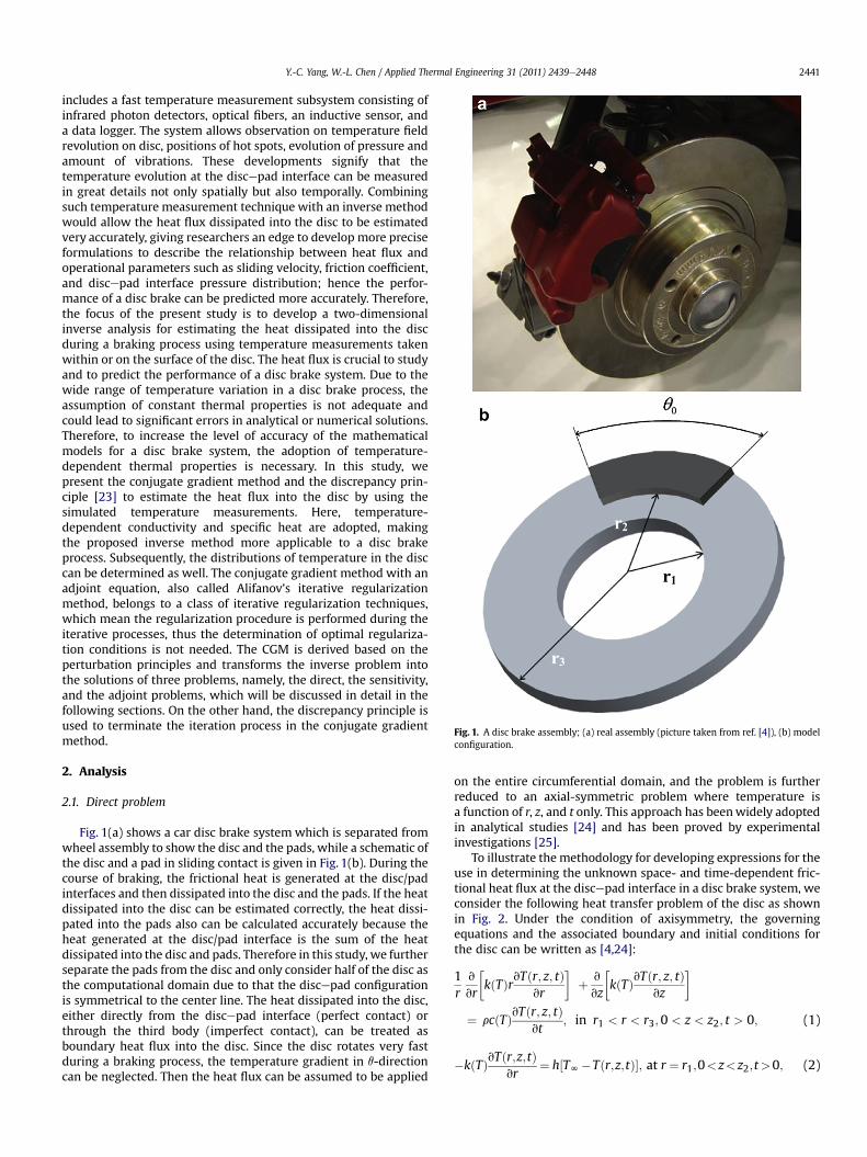
Fig. 1. A disc brake assembly; (a) real assembly (picture taken from ref. [4]), (b) modelconfiguration.

Y.-C. Yang, W.-L. Chen / Applied Thermal Engineering 31 (2011) 2439e2448 2441

includes a fast temperature measurement subsystem consisting ofinfrared photon detectors, optical fibers, an inductive sensor, anda data logger. The system allows observation on temperature fieldrevolution on disc, positions of hot spots, evolution of pressure andamount of vibrations. These developments signify that thetemperature evolution at the discepad interface can be measuredin great details not only spatially but also temporally. Combiningsuch temperature measurement technique with an inverse methodwould allow the heat flux dissipated into the disc to be estimatedvery accurately, giving researchers an edge to develop more preciseformulations to describe the relationship between heat flux andoperational parameters such as sliding velocity, friction coefficient,and discepad interface pressure distribution; hence the perfor-mance of a disc brake can be predicted more accurately. Therefore,the focus of the present study is to develop a two-dimensionalinverse analysis for estimating the heat dissipated into the discduring a braking process using temperature measurements takenwithin or on the surface of the disc. The heat flux is crucial to studyand to predict the performance of a disc brake system. Due to thewide range of temperature variation in a disc brake process, theassumption of constant thermal properties is not adequate andcould lead to significant errors in analytical or numerical solutions.Therefore, to increase the level of accuracy of the mathematicalmodels for a disc brake system, the adoption of temperature-dependent thermal properties is necessary. In this study, wepresent the conjugate gradient method and the discrepancy prin-ciple [23] to estimate the heat flux into the disc by using thesimulated temperature measurements. Here, temperature-dependent conductivity and specific heat are adopted, makingthe proposed inverse method more applicable to a disc brakeprocess. Subsequently, the distributions of temperature in the disccan be determined as well. The conjugate gradient method with anadjoint equation, also called Alifanov’s iterative regularizationmethod, belongs to a class of iterative regularization techniques,which mean the regularization procedure is performed during theiterative processes, thus the determination of optimal regulariza-tion conditions is not needed. The CGM is derived based on theperturbation principles and transforms the inverse problem intothe solutions of three problems, namely, the direct, the sensitivity,and the adjoint problems, which will be discussed in detail in thefollowing sections. On the other hand, the discrepancy principle isused to terminate the iteration process in the conjugate gradientmethod.

2. Analysis

2.1. Direct problem

Fig. 1(a) shows a car disc brake system which is separated fromwheel assembly to show the disc and the pads, while a schematic ofthe disc and a pad in sliding contact is given in Fig. 1(b). During thecourse of braking, the frictional heat is generated at the disc/padinterfaces and then dissipated into the disc and the pads. If the heatdissipated into the disc can be estimated correctly, the heat dissi-pated into the pads also can be calculated accurately because theheat generated at the disc/pad interface is the sum of the heatdissipated into the disc and pads. Therefore in this study, we furtherseparate the pads from the disc and only consider half of the disc asthe computational domain due to that the discepad configurationis symmetrical to the center line. The heat dissipated into the disc,either directly from the discepad interface (perfect contact) orthrough the third body (imperfect contact), can be treated asboundary heat flux into the disc. Since the disc rotates very fastduring a braking process, the temperature gradient in q-directioncan be neglected. Then the heat flux can be assumed to be applied

on the entire circumferential domain, and the problem is furtherreduced to an axial-symmetric problem where temperature isa function of r, z, and t only. This approach has beenwidely adoptedin analytical studies [24] and has been proved by experimentalinvestigations [25].

To illustrate the methodology for developing expressions for theuse in determining the unknown space- and time-dependent fric-tional heat flux at the discepad interface in a disc brake system, weconsider the following heat transfer problem of the disc as shownin Fig. 2. Under the condition of axisymmetry, the governingequations and the associated boundary and initial conditions forthe disc can be written as [4,24]:

1r

v

vr

�kðTÞrvTðr; z; tÞ

vr

�þ v

vz

�kðTÞvTðr; z; tÞ

vz

�

¼ rcðTÞvTðr; z; tÞvt

; in r1 < r < r3;0 < z < z2; t > 0; (1)

�kðTÞvTðr;z;tÞvr

¼ h½TN�Tðr;z;tÞ�; at r ¼ r1;0< z< z2;t>0; (2)

Fig. 2. Schematic of the disc.

Y.-C. Yang, W.-L. Chen / Applied Thermal Engineering 31 (2011) 2439e24482442

kðTÞvTðr;z;tÞvr

¼ h½TN�Tðr;z;tÞ�; at r ¼ r3;0<z< z2;t>0; (3)

kðTÞvTðr; z; tÞvz

¼ 0 at z ¼ 0; r1 < r < r3; t > 0; (4)

kðTÞvTðr;z;tÞvz

¼ h½TN�Tðr;z;tÞ�; at z¼ z2;r1< r< r2;t>0; (5)

kðTÞvTðr; z; tÞvz

¼ qðr; tÞ at z ¼ z2; r2 < r < r3; t > 0; (6)

Tðr; z;0Þ ¼ T0; for r1 < r < r3;0 < z < z2; t ¼ 0; (7)

where TN is the surrounding temperature and T0 is the initialtemperature. r is the density, k(T) and c(T)are the temperature-dependent thermal conductivity and specific heat, respectively,while h is the convection heat transfer coefficient at the outersurfaces. q(r,t) in Eq. (6) is the frictional heat flux into the disc. If thecontact pressure between the pad and disc is assumed constant, thefrictional heat flux is a function of time and space variable r. This isbecause work done by friction force grows as r increases. However,if uniform wear contact is adopted, the frictional heat flux is justa function of time and is independent of the space variable r.

The direct problem considered here is concerned with thedetermination of themedium temperaturewhen the frictional heatflux q(r,t), thermo-physical properties of the disc, and initial andboundary conditions are known.

2.2. Inverse problem

For the inverse problem, the function q(r,t) is regarded as beingunknown, while everything else in Eqs. (1)e(7) is known. Inaddition, temperature readings taken within the disc are consid-ered available. The objective of the inverse analysis is to predict theunknown space- and time-dependent function of frictional heatflux, q(r,t), merely from the knowledge of these temperaturereadings. Let the measured temperature at the measurementposition ðr; zÞ ¼ ðri; zmÞ and time t be denoted by Yiðri; zm; tÞ,i¼ 1eM, whereM represents the number of thermocouples and zmis the z coordinate of all the thermocouples. Then this inverseproblem can be stated as follows: by utilizing the above mentionedmeasured temperature data Yiðri; zm; tÞ, the unknown q(r,t) is to beestimated over the specified space and temporal domain.

The solution of the present inverse problem is to be obtained insuch a way that the following functional is minimized:

J½qðr; tÞ� ¼Ztft¼0

XMi¼1

½Tiðri; zm; tÞ � Yiðri; zm; tÞ�2dt; (8)

where Tiðri; zm; tÞ is the estimated (or computed) temperature atthe measurement location ðr; zÞ ¼ ðri; zmÞ. In this study, Tiðri; zm; tÞare determined from the solution of the direct problem givenpreviously by using an estimated qKðr; tÞ for the exact qðr; tÞ, hereqKðr; tÞ denotes the estimated quantities at the Kth iteration. tf isthe final time of measurement. In addition, in order to developexpressions for the determination of the unknown q(r,t), a “sensi-tivity problem” and an “adjoint problem” are constructed asdescribed below.

2.3. Sensitivity problem and search step size

The sensitivity problem is obtained from the original directproblem defined by Eqs. (1)e(7) in the following manner: It isassumed that when q(r,t) undergoes a variation q(r,t), T(r,z,t), k(T),and c(T) are perturbed by DT, Dk, and Dc, respectively. Thenreplacing in the direct problem q(r,t) by qðr; tÞ þ Dqðr; tÞ, T by TþDT,k(T) by k(T)þDk, and c(T) by c(T)þDc, subtracting from theresulting expressions the direct problem, using the fact thatDk ¼ ½dkðTÞ=dT�DT and Dc ¼ ½dcðTÞ=dT �DT , and neglecting thesecond-order terms, the following sensitivity problem for thesensitivity function DT can be obtained.

1r

v

vr

�rv

vr½kðTÞDTðr; z; tÞ�

�þ v2

vz2½kðTÞDTðr; z; tÞ�

¼ v

vt½rcðTÞDTðr; z; tÞ�; in r1 < r < r3;0 < z < z2; t > 0; (9)

v

vr½kðTÞDTðr;z;tÞ� ¼ hDTðr;z;tÞ; at r ¼ r1;0<z< z2;t>0; (10)

v

vr½kðTÞDTðr;z;tÞ� ¼ �hDTðr;z;tÞ; at r ¼ r3;0< z< z2;t>0; (11)

v

vz½kðTÞDTðr; z; tÞ� ¼ 0; at z ¼ 0; r1 < r < r3; t > 0; (12)

Y.-C. Yang, W.-L. Chen / Applied Thermal Engineering 31 (2011) 2439e2448 2443

v

vz½kðTÞDTðr;z;tÞ� ¼ �hDTðr;z;tÞ; at z¼ z2;r1< r< r2;t>0; (13)

v

vz½kðTÞDTðr;z;tÞ� ¼ Dqðr;tÞ; at z¼ z2;r2< r< r3;t>0; (14)

DTðr; z;0Þ ¼ 0; for r1 < r < r3;0 < z < z2; t ¼ 0: (15)

The sensitivity problem of Eqs. (9)e(15) can be solved by thesame method as the direct problem of Eqs. (1)e(7).

2.4. Adjoint problem and gradient equation

To formulate the adjoint problem, Eq. (1) is multiplied by theLagrange multiplier (or adjoint function) l, and the resultingexpressions are integrated over the time and correspondent spacedomains. Then the results are added to the right hand side of Eq. (8)to yield the following expression for the functional J½qðr; tÞ�:

J½qðr; tÞ� ¼Ztf

t¼0

Zz2z¼0

Zr3r¼r1

XMi¼1

½Tiðr; z; tÞ

� Yiðr; z; tÞ�2dðr � riÞdðz� zmÞdrdzdt

þZtf

t¼0

Zz2z¼0

Zr3r¼r1

r$lðr; z; tÞ$�1r

v

vr

�kðTÞrvT

vr

�

þ v

vz

�kðTÞvT

vz

�� rcðTÞvT

vt

�drdzdt (16)

where dð,Þ is the Dirac function. The variation DJ is derived byperturbing q(r,t) by qðr; tÞ þ Dqðr; tÞ, T by TþDT, k(T) by k(T)þDk,and c(T) by c(T)þDc, respectively, in Eq. (16). Subtracting from theresulting expressions the original Eq. (16), using the fact that Dk ¼½dkðTÞ=dT�DT and Dc ¼ ½dcðTÞ=dT �DT , and neglecting the second-order terms, we thus find:

DJ½qðr; tÞ� ¼Ztft¼0

Zz2z¼0

Zr3r¼r1

XMi¼1

2½Tiðr; z; tÞ

� Yiðr; z; tÞ�DTdðr � riÞdðz� zmÞdrdzdt

þZtft¼0

Zz2z¼0

Zr3r¼r1

l$

(v

vr$r$

v

vr½kðTÞDT �

þ r$v2

vz2½kðTÞDT � � r$

v

vt½rcðTÞDT �

)drdzdt (17)

We can integrate the second triple-integral term in Eq. (17) byparts, utilizing the initial and boundary conditions of the sensitivityproblem. Then DJ is allowed to go to zero. The vanishing of theintegrands containing DT leads to the following adjoint problem forthe determination of lðr; z; tÞ:

1r$kðTÞ$ v

vr

�rvlðr; z; tÞ

vr

�þ kðTÞ$v

2lðr; z; tÞvz2

þ rcðTÞvlðr; z; tÞvt

þ 1r$XMi¼1

2½Tiðr; z; tÞ � Yiðr; z; tÞ�dðr � riÞdðz� zmÞ

¼ 0; in r1 < r < r3;0 < z < z2; t > 0; (18)

kðTÞvlðr; z; tÞvr

¼ hlðr; z; tÞ; at r ¼ r1;0 < z < z2; t > 0; (19)

kðTÞvlðr; z; tÞvr

¼ �hlðr; z; tÞ at r ¼ r3;0 < z < z2; t > 0; (20)

kðTÞvlðr; z; tÞvz

¼ 0 at z ¼ 0; r1 < r < r3; t > 0; (21)

kðTÞvlðr; z; tÞvz

¼ �hlðr; z; tÞ at z ¼ z2; r1 < r < r2; t > 0; (22)

kðTÞvlðr; z; tÞvz

¼ 0 at z ¼ z2; r2 < r < r3; t > 0; (23)

lðr; z; tÞ ¼ 0 for r1 < r < r3;0 < z < z2; t ¼ tf : (24)

The adjoint problem is different from the standard initial valueproblem in that the final time condition at time t¼ tf is specifiedinstead of the customary initial condition at time t¼ 0. However,this problem can be transformed to an initial value problem by thetransformation of the time variable as s ¼ tf � t. Then the adjointproblem can be solved by the same method as the direct problem.

Finally the following integral term is left:

DJ ¼Ztft¼0

Zr3r¼r2

rlðr; z2; tÞDqðr; tÞdrdt: (25)

From the definition used in Ref. [7], we have:

DJ ¼Ztft¼0

Zr3r¼r2

rJ0ðr; tÞDqðr; tÞdrdt; (26)

where J0(t) is the gradient of the functional J(q). A comparison ofEqs. (25) and (26) leads to the following form:

J0ðr; tÞ ¼ lðr; z2; tÞ: (27)

2.5. Conjugate gradient method for minimization

The following iteration process based on the conjugate gradientmethod is now used for the estimation of q(r,t) by minimizing theabove functional J[q(r,t)]:

qKþ1ðr; tÞ ¼ qKðr; tÞ � bKpK�r; t�; K ¼ 0;1;2;.; (28)

where bK is the search step size in going from iteration K to iterationKþ1, and pK(r,t) is the direction of descent (i.e., search direction)given by:

pKðr; tÞ ¼ J0Kðr; tÞ þ gKpK�1�r; t�; (29)

which is conjugation of the gradient direction J0Kðr; tÞ at iteration Kand the direction of descent pK�1ðr; tÞ at iteration K� 1. Theconjugate coefficient gK is determined from:

gK ¼

Ztft¼0

XMi¼1

hJ0Kðri; tÞ

i2dt

Ztft¼0

XMi¼1

hJ0K � 1ðri; tÞ

i2dt

with g0 ¼ 0: (30)

Table 1Brake dimensions and operating conditions.

Inner disc diameter 0.132 (m)Outer disc diameter 0.227 (m)Mean sliding radius 0.094.5 (m)Sliding length 0.037 (m)Disc thickness 0.011 (m)Pad thickness 0.010 (m)Initial speed 100 (kmh�1)Braking time 3.96 (s)Deceleration 7 (ms�2)Total energy 165 (kJ)Convection coefficient 60 (Wm�2 K�1)

Y.-C. Yang, W.-L. Chen / Applied Thermal Engineering 31 (2011) 2439e24482444

The convergence of the above iterative procedure in minimizingthe functional J is proved in Ref. [7]. To perform the iterationsaccording to Eq. (28), we need to compute the step size bK and thegradient of the functional J0Kðr; tÞ.

The functional J½qKþ1ðr; tÞ� for iteration Kþ 1 is obtained byrewriting Eq. (8) as:

JhqKþ1ðr;tÞ

i¼Ztft¼0

XMi¼1

hTi�qK �bKpK

��Yiðri;zm;tÞ

i2dt; (31)

where we replace qKþ1 by the expression given by Eq. (28). Iftemperature TiðqK �bKpKÞ is linearized by a Taylor expansion, Eq.(31) takes the form:

JhqKþ1ðr; tÞ

i¼

Ztft¼0

XMi¼1

hTiðqKÞ � bKDTiðpKÞ

� Yiðri; zm; tÞi2dtdt; ð32Þ

where TiðqKÞ is the solution of the direct problem at ðr; zÞ ¼ ðri; zmÞby using estimated qK(r,t) for exact q(r,t) at time t. The sensitivityfunction DTiðpKÞ is taken as the solution of Eqs. (9)e(15) at themeasured position ðr; zÞ ¼ ðri; zmÞ by letting Dq¼ pK [7]. The searchstep size bK is determined byminimizing the functional given by Eq.(32) with respect to bK. The following expression can be obtained:

bK ¼

Ztft¼0

XMi¼1

DTi�pK�h

Ti�qK�� Yi

idt

Ztft¼0

XMi¼1

hDTiðpKÞ

i2dt

: (33)

2.6. Stopping criterion

If the problem contains no measurement errors, the traditionalcheck condition specified as

J�qKþ1

�< h; (34)

where h is a small specified number, can be used as the stoppingcriterion. However, the observed temperature data containsmeasurement errors; as a result, the inverse solution will tend toapproach the perturbed input data, and the solution will exhibitoscillatory behavior as the number of iteration is increased [26].Computational experience has shown that it is advisable to use thediscrepancyprinciple [23] for terminating the iterationprocess in theconjugate gradient method. Assuming Tiðri; zm; tÞ � Yiðri; zm; tÞys,the stopping criteria h by the discrepancy principle can be obtainedfrom Eq. (8) as

h ¼ Ms2tf ; (35)

where s is the standard deviation of the measurement error. Thenthe stopping criterion is given by Eq. (34) with h determined fromEq. (35). The computational procedure is the same as in [20], hencethere is no need to repeat here.

Table 2Thermo-physical properties of disc and pad.

Disc Pad

Conductivity (Wm�1 K�1) 43.5 12Density (kgm�3) 7850 2500Specific heat (J kg�1 K�1) 445 900

3. Results and discussion

A bench-mark test case in [24] is first considered to validate thecode used in this study. The details of the dimensions and operatingconditions are given in Tables 1 and 2. In this test case, the thermal

properties are taken as constant. Furthermore, under the assump-tion of constant deceleration and uniform wear contact betweenthe pad and the disc, the boundary heat flux in Eq. (6) is a functionof time only and can be written as:

qðtÞ ¼ q0

1� t

tf

!; (36)

with

q0 ¼ q02p

mfpmaxr2u0; (37)

where pmax is themaximumpressure distributed in the pad and f isthe heat partition coefficient between the disc and the pad definedas:

f ¼ xdSdxdSd þ xpSp

; (38)

where xd and xP are the thermal effusivities of the disc and the pad,and Sd and Sp are frictional contact surfaces of the disc and the pad,respectively. Thermal effusivity x is defined as x ¼

ffiffiffiffiffiffiffiffikrc

p.

The numerical procedure in this paper is based on theunstructured-mesh, fully collocated,finite-volumecode, ‘USTREAM’

developed by W.-L. Chen. This is the descendent of the structured-mesh, multi-block code of ‘STREAM’ [27]. The computational meshconsists of 860 cells, where there are 20 and 43 cells, respectively,in the z- and r-directions. This mesh has been proved in a grid-independent test to achieve grid-independent solutions. Thecomparison ofmean sliding radius surface temperature variations isgiven in Fig. 3. To find an appropriate time-step interval to achievetime-step-interval independent solutions, the results are computedbyusing threedifferent numbers of time steps, namely 100, 200, and300. It can be seen that the results by the three time-step numbersare almost identical and are in very good agreement with New-comb’s analytical solution. This indicates that the time step numberof 100, corresponding to a time-step interval of 0.0396 s, is goodenough to ensure time-step-interval independent solutions in thisproblem. In addition, the test also versifies the correctness of thecode used in this study.

To test the effect of adopting temperature-dependent thermo-physical properties, the disc is assumed made of AISI-1045 steel,which is commonly used in friction elements. Since the densityof AISI-1045 steel has relatively weak temperature dependence

Fig. 3. Comparison disc mean sliding radius surface temperature variations.

a

b

Fig. 4. Measured AISI-1045 steel specific heat and thermal conductivity variationsagainst temperature. (a) Specific heat variations, and (b) thermal conductivityvariations.

Y.-C. Yang, W.-L. Chen / Applied Thermal Engineering 31 (2011) 2439e2448 2445

over a wide temperature range [28], a constant average value of7844 kgm�3 is adopted. However, the specific heat and thermaldiffusivity from the experimental measurements of Touloukian [29]are used here, and Fig. 4 shows the variations of specific heat andthermal conductivity with respect to temperature from 280 K to1300 K. The mean sliding radius temperature variations computedwith temperature-dependent thermo-physical properties are alsoshown in Fig. 3. Although the results are not significantly differentfrom those adopting constant thermo-physical properties, the de-viation, about 5 K at most places, is clearly present. To ensure highlevel of accuracy, temperature-dependent thermo-physical prop-erties should be used, and in the following, all results were obtainedusing temperature-dependent thermo-physical properties.

The objective of this article is to validate the current approachwhen used in estimating the unknown heat flux into the discduring a braking process accurately with no prior information onthe functional form of the unknown quantities, a procedure calledfunction estimation. In this study, we did not have an experimentsetup to measure the temperatures on the disc. Instead, we sub-stitute an assumed interface heat flux such as Eq. (36) into thedirect problem of Eqs. (1)e(7) to calculate the temperatures atthe locations where the temperature measurements are taken.The results are termed the computed temperature Yexactðri; zm; tÞ.However, in reality, temperature measurements always containsome degree of error, whose magnitude depends upon the partic-ular measuring method employed. To take measurement errorsinto account, a random error noise is added to the above computedtemperature Yexactðri; zm; tÞ to obtain the measured temperatureYiðri; zm; tÞ. Hence, the measured temperature Yiðri; zm; tÞ isexpressed as:

Yiðri; zm; tÞ ¼ Yexactðri; zm; tÞ þ6s; (39)

where 6 is a random variable within �2.576 to 2.576 for a 99%confidence bounds, and s is the standard deviation of themeasurement. The measured temperature Yiðri; zm; tÞ generated insuch way is called the simulated measurement temperature. Atfirst, the temperature measurement is assumed located atzm¼ 0.0054 m, equivalent to 0.1 mm inside the disc, and along thefriction interface (see Fig. 2). The comparison between the inverseand exact heat flux, using Eq. (36), at three different time steps isgiven in Fig. 5. The inverse results were obtained with an initialguess of q0(r,t)¼ 1.0�105 Wm�2 and measurement errors s¼ 0.0.

Fig. 5 shows that for this simple heat flux function, the inverseestimation is almost identical to the exact value. Next, we adopt theuniform pressure assumption in Talati and Jalalifar [4], where theheat flux function is written as:

qðr; tÞ ¼ q0

rr2

1� t

tf

!; (40)

Eq. (40) indicates that the heat flux is now a function of radiusand time. The results at three different time steps are shown inFig. 6, and yet again very good agreement between the inverse andthe exact values can be seen. Here the inverse results were obtainedwith an initial guess of q0(r,t)¼ 1.0�105 Wm�2 and measurementerrors s¼ 0.0. Once the heat flux has been estimated correctly, thetemperature evolution anywhere on the disc can be calculatedaccurately too. This is shown in Fig. 7, where the comparison oftemperature evolution at four different locations on the disc surfaceis given. It is noticeable that the variations of calculated and exacttemperature are almost identical.

Fig. 5. Estimated q(t) (Eq. (37)) with zm¼ 0.0054 m, the initial guess q0(r,t)¼1.0�105 Wm�2, and measurement error s¼ 0.0. Fig. 7. Estimated disc surface temperature variations at 4 different radial positions

with zm¼ 0.0054 m, the initial guess q0(r,t)¼ 1.0�105 Wm�2, and measurement errors¼ 0.0.

Y.-C. Yang, W.-L. Chen / Applied Thermal Engineering 31 (2011) 2439e24482446

In order to investigate the influence of measurement error uponthe estimated results, Fig. 8 shows the estimated values of theunknown function q(r,t), obtained with the initial guesses q0(r,t)¼1.0�105 Wm�2, andmeasurement error of deviations¼ 0.005. Thedeviation s¼ 0.005 corresponds to 1.28% of measurement error,which is roughly in the range of 4e6 K over the entire disc surfacetemperature variation during the braking process. This magnitudeof temperature measurement error is huge according to the accu-racy standard of modern thermal couples, whose precision is nor-mally within �1 K. Despite this unrealistically large measurementerror, the results indicate that this temperature measurement errorin general creates only about 2% of error on heat flux magnitude,demonstrating that the accuracy of the current method is not verysensitive to temperature measurement error.

Since thedirect problem is a transientheat transferproblem, therehave been studies reporting the sensitivity of inverse accuracy on therelativedistancebetween theestimatedandmeasurement quantitiesin inverse transient heat conduction problems [30]. Under some

Fig. 6. Estimated q(r,t) (Eq. (40)) with zm¼ 0.0054 m, the initial guess q0(r,t)¼1.0�105 Wm�2, and measurement error s¼ 0.0.

circumstances, the accuracy deteriorates rapidly as themeasurementlocationmoves away from the estimated quantity location. Thereforein the current inverse problem, this issue needs to be investigated. Toexamine the sensitivity of inverse method’s accuracy on measure-ment location, the thermal couple is assumed to be located resp-ectively at three other positions, zm¼ 0.005 m, 0.0035 m, and0.0001 m. The estimated heat flux distributions, together with thoseof zm¼ 0.0054 m, are plotted in Fig. 9. These resultswere all obtainedwith an initial guess of q0(r,t)¼ 1.0�105 Wm�2 and measurementerrors s¼ 0.0, and they obviously show that the inverse accuracydeteriorates progressively as the measurement positionmoves awayfrom the friction interface, especially at the vicinity of r¼ r2. In thecase of zm¼ 0.0001 m, the inverse heat flux at t¼ 3.66 s is in generalhalf the magnitude of the exact value, resulting in an discrepancyeven larger than that produced by taking measurement error intoaccount.

Fig. 8. Estimated q(r,t) (Eq. (40)) with zm¼ 0.0054 m, the initial guess q0(r,t)¼1.0� 105 Wm�2, and measurement error s¼ 0.005.

Fig. 9. Estimated q(r,t) (Eq. (40)) with four different measurement locations, the initialguess q0(r,t)¼ 1.0� 105 Wm�2, and measurement error s¼ 0.0.

a

b

Fig. 10. The heat flux function taken from Choi and Lee [2]; (a) exact q(r,t) distribu-tions, and (b) inverse q(r,t) distributions.

Fig. 11. Estimated q(r,t) (Eq. (41)) with zm¼ 0.0054 m, the initial guess q0(r,t)¼1.0�105 Wm�2, and measurement error s¼ 0.0.

Y.-C. Yang, W.-L. Chen / Applied Thermal Engineering 31 (2011) 2439e2448 2447

In order to demonstrate the capability of the present method inobtaining an accurate estimation of arbitrary form of the unknownheat flux, we consider another case of q(r,t), based on the ther-moelastic simulation in Choi and Lee [2], which is calculated by:

qðr; tÞ ¼ mruðtÞpðr; tÞ; (41)

where u(t) and p(r,t) are distributions taken from Figs. 4 and 6 in[2]. The heat generation during the braking stage is shown inFig. 10(a). Please note that due to data digitizing and scaling factors,the absolute magnitude of heat flux shown here is not identical tothat in [2] but the tendency of data variation is preserved. In theirstudy, heat conduction and elastic equations are coupled throughthe heat generated at discepad interface calculated by Eq. (41).Therefore, the current inverse method can be applied to thermo-elastic approach to estimate the heat flux into the disc and thenevaluate the heat partition between the disc and pad at the frictioninterface. Fig. 10(b) shows the estimated results of q(r,t), obtainedwith zm¼ 0.0054 m, the initial guesses q0(r,t)¼ 1.0�105 Wm�2,and measurement error of deviation s¼ 0.0. Excellent agreementbetween the exact and inverse heat flux can be seen by comparingFig. 10(a) and (b). More detailed comparison on the heat fluxdistributions along the radial direction at three different time stepsgiven in Fig. 11 further confirms the accuracy of the inverse esti-mation. The results indicate that the current inverse methodperforms very well even on this highly complicated heat fluxfunction.

4. Conclusion

An inverse algorithm based on the conjugate gradient methodand the discrepancy principle was successfully applied for the solu-tion of the inverse problem to determine the unknown space- andtime-dependent heat flux into the disc during a braking process,while knowing the temperature history at some measurementlocations.Due to thewide rangeof temperature variation inabrakingprocess, temperature-dependent specific heat and thermal conduc-tivity are used here; hence the governing equation of the directproblem becomes nonlinear. Numerical results confirm that themethod proposed herein can accurately estimate the space- andtime-dependent heat flux and temperature distributions for theproblem even involving the inevitable measurement errors. The

Y.-C. Yang, W.-L. Chen / Applied Thermal Engineering 31 (2011) 2439e24482448

proposed inverse algorithm does not require prior information forthe functional formof theunknownquantities toperform the inversecalculation, and excellent estimated values can be obtained for theconsidered problem. However, the results also show that the inverseaccuracy is very sensitive to the distance between the estimated andmeasurement quantities. The temperature measurement locationshould be put as close to the friction interface as possible because theaccuracy of the inverse method deteriorates rapidly as the mea-surement location moves away from the friction interface.

Acknowledgements

This work was supported by the National Science Council,Taiwan, Republic of China, under the grant numbers NSC 98-2221-E-168-035 and NSC 98-2221-E-168-034.

References

[1] P. Dufrenoy, Two-/three-dimensional hybrid model of the thermomechanicalbehavior of disc brakes, Proc. IMechE Part F: J. Rail Rapid Transit. 218 (2004)17e30.

[2] J.H. Choi, I. Lee, Finite element analysis of transient thermoelastic behaviors indisc brakes, Wear 257 (2004) 47e58.

[3] C.H. Gao, X.Z. Lin, Transient temperature field analysis of a brake in a non-axisymmetric three-dimensional model, J. Mater. Process. Technol. 129(2002) 513e517.

[4] F. Talati, S. Jalalifar, Analysis of heat conduction in a disk brake system, HeatMass Transfer 45 (2009) 1047e1059.

[5] N. Laraqi, Phenomene de constriction thermique dans les contacts glissants(thermal constriction phenomenon in sliding contacts), Int. J. Heat MassTransfer 39 (1996) 3717e3724.

[6] D. Majcherczak, P. Dufrenoy, M. Nait-Abdelaziz, Third body influence onthermal friction contact problems: application to braking, ASME J. Tribol. 127(2005) 89e95.

[7] O.M. Alifanov, Inverse Heat Transfer Problem. Springer-Verlag, New York, 1994.[8] C.H. Huang, C.C. Shih, A shape identification problem in estimating simulta-

neously two interfacial configurations in a multiple region domain, Appl.Therm. Eng. 26 (2006) 77e88.

[9] Y.C. Yang, Simultaneously estimating the contact heat and mass transfercoefficients in a double-layer hollow cylinder with interface resistance, Appl.Therm. Eng. 27 (2007) 501e508.

[10] H.T. Chen, H.C. Wang, Estimation of heat-transfer characteristics on a rectan-gular fin underwet conditions, Int. J. Heat Mass Transfer 51 (2008) 2123e2138.

[11] W.L. Chen, Y.C. Yang, S.S. Chu, Estimation of heat generation at the interface ofcylindrical bars during friction process, Appl. Therm. Eng. 29 (2009) 351e357.

[12] Y.C. Yang, W.L. Chen, An iterative regularization method in simultaneouslyestimating the inlet temperature and heat-transfer rate in a forced-convectionpipe, Int. J. Heat Mass Transfer 52 (2009) 1928e1937.

[13] W.L. Chen, Y.C. Yang, Simultaneous estimation of heat-transfer rate andcoolant fluid velocity in a transpiration cooling process, Int. J. Therm. Sci. 49(2010) 1407e1416.

[14] C. Le Niliot, F. Lefevre, Multiple transient point heat sources identification inheat diffusion: application to numerical two- and three-dimensional prob-lems, Numer. Heat Transfer Part B 39 (2001) 277e301.

[15] M. Raudensky, K.A. Woodbury, J. Kral, Genetic algorithm in solution of inverseheat conduction problems, Numer. Heat Transfer Part B 28 (1995) 293e306.

[16] C. Le Niliot, F. Lefevre, A parameter estimation approach to solve the inverseproblem of point heat sources identification, Int. J. Heat Mass Transfer 47(2004) 827e841.

[17] C.H. Huang, H.C. Lo, A three-dimensional inverse problem in estimating theinternal heat flux of housing for high speed motors, Appl. Therm. Eng. 26(2006) 1515e1529.

[18] H.L. Lee, W.J. Chang, W.L. Chen, Y.C. Yang, An inverse problem of estimatingthe heat source in tapered optical fibers for scanning near-field opticalmicroscopy, Ultramicroscopy 107 (2007) 656e662.

[19] B. Jin, L. Marin, The method of fundamental solutions for inverse sourceproblems associated with the steady-state heat conduction, Int. J. Numer.Methods Eng. 69 (2007) 1570e1589.

[20] W.L. Chen, Y.C. Yang, Inverse problem of estimating the heat flux at the roller/workpiece interface during a rolling process, Appl. Therm. Eng. 30 (2010)1247e1254.

[21] J. Thevenet, M. Siroux, B. Desmet, Measurements of brake disc surfacetemperature and emissivity by two-color pyrometry, Appl. Therm. Eng. 30(2010) 753e759.

[22] P. Litos, M. Honner, V. Lang, J. Bartik, M. Hynek, A measuring system forexperimental research on the thermomechanical coupling of disc brakes, Proc.IMechE, Part D: J. Automobile Eng. 222 (2008) 1247e1257.

[23] O.M. Alifanov, E.A. Artyukhin, Regularized numerical solution of nonlinearinverse heat-conduction problem, J. Eng. Phys. 29 (1975) 934e938.

[24] T.P. Newcomb, Transient temperatures attained in disk brakes, Br. J. Appl.Phys. 10 (1959) 339e340.

[25] D. Majcherczak, P. Dufrenoy, Y. Berthier, Tribological, thermal and mechanicalcoupling aspects of the dry sliding contact, Tribol. Int. 40 (2007) 834e843.

[26] O.M. Alifanov, Application of the regularization principle to the formulation ofapproximate solution of inverse heat conduction problem, J. Eng. Phys. 23(1972) 1566e1571.

[27] F.S. Lien, W.L. Chen, M.A. Leschziner, A multiblock implementation of a non-orthogonal, collocated finite volume algorithm for complex turbulent flows,Int. J. Numer. Methods Fluids 23 (1996) 567e588.

[28] R.D. Pelhlke, A. Jeyarajan, H. Wada, Report No. NSF/MAE-82028, NSF AppliedResearch Division, University of Michigan (1982).

[29] Y.S. Touloukian, Thermophysical Properties of High Temperature SolidMaterials. Macmillan, New York, 1967.

[30] W.L. Chen, Y.C. Yang, Inverse prediction of frictional heat flux and tempera-ture in sliding contact with a protective strip by iterative regularizationmethod, Appl. Math. Model. 35 (2011) 2874e2886.