1

A Nonlinear Interface Element for 3D Mesoscale Analysis

of Brick-Masonry Structures

L. Macorini1, B.A. Izzuddin

2

Abstract

This paper presents a novel interface element for the geometric and material nonlinear

analysis of unreinforced brick-masonry structures. In the proposed modelling approach, the

blocks are modelled using 3D continuum solid elements, while the mortar and brick-mortar

interfaces are modelled by means of the 2D nonlinear interface element. This enables the

representation of any 3D arrangement for brick-masonry, accounting for the in-plane stacking

mode and the through-thickness geometry, and importantly it allows the investigation of both

the in-plane and the out-of-plane response of unreinforced masonry panels. A co-rotational

approach is employed for the interface element, which shifts the treatment of geometric

nonlinearity to the level of discrete entities, and enables the consideration of material

nonlinearity within a simplified local framework employing first-order kinematics. In this

respect, the internal interface forces are modelled by means of elasto-plastic material laws

based on work-softening plasticity and employing multi-surface plasticity concepts.

Following the presentation of the interface element formulation details, several experimental-

numerical comparisons are provided for the in-plane and out-of-plane static behaviour of

brick-masonry panels. The favourable results achieved demonstrate the accuracy and the

significant potential of using the developed interface element for the nonlinear analysis of

brick-masonry structures under extreme loading conditions.

Keywords: non linear interface element, cohesive model, multi-surface plasticity, geometric

nonlinearity, brick-masonry, in-plane and out-of-plane behaviour.

1 Marie Curie Research Fellow, Department of Civil and Environmental Engineering, Imperial College London.

2 Professor of Computational Structural Mechanics, Department of Civil and Environmental Engineering,

Imperial College London.

2

Introduction

Nonlinear interface elements represent an effective tool to model interaction among different

constitutive components of solids and to capture failure mechanisms in a large variety of

structural systems. Interface elements were initially employed for simulating discontinuities

in rock mechanics [1] and cracks in brittle materials like concrete [2], while more recently

they have been used to model delamination and fracture in multi-layered composites [3,4].

In order to accurately reproduce most of the physical phenomena associated with interface

failure, the interface elements have to be coupled with accurate material models that relate

tractions with separation displacements. Some main features of such constitutive relations

were introduced in the first cohesive zone models tailored to analyse crack propagation in

either ductile or brittle materials (a detailed review can be found in [5]). At present, the most

advanced cohesive models are based on either softening plasticity [6] or damage mechanics

[7]. They account for the interaction between opening and sliding fracture modes and allow

the description of delamination, decohesion and loss of friction at the interfaces between

different bodies and at the fracture process zones in solid elements.

The use of interface elements is particularly effective when the locus of potential damage and

fracture is known a priori, which is typically related to the inherent texture of the analysed

structure. This is the case for unreinforced brick-masonry (URM) where bricks are arranged

in an orderly manner so as to form structural elements. Experimental outcomes [8] and

inspection of failure modes of real URM structures show that cracks usually run along brick-

mortar interfaces and can then continue through bricks following continuous paths. These

intrinsic features of the brick-masonry structural behaviour suggested the use of nonlinear

interface elements for detailed finite element analyses of URM panels under monotonic and

cyclic loads [9,10]. In such structural models zero-thickness interfaces are employed to

represent the nonlinear behaviour of mortar and brick-mortar interface as well as potential

3

cracks in bricks. Damage and fracture are assumed to occur at the interfaces only, whereas

the connected continuous elements are characterized by a linear elastic behaviour.

Most of the mesoscale models for URM developed so far, account for the in-plane stacking

mode of bricks and mortar only, and are aimed at investigating the in-plane nonlinear

response of masonry walls. Such models cannot be effectively employed to assess the

structural performance under complex loading conditions as in the case of earthquakes, when

panels in URM buildings are loaded simultaneously by both in-plane and out-of-plane

actions.

In order to define more general analysis tools for mesoscale analysis of URM elements

characterized by complex brick arrangements (quarry masonry, multi-leaf walls, etc.), both

the in-plane stacking mode and the through-thickness geometry should be represented. Just a

few models, presented very recently, consider a detailed description for the 3D texture of

URM. These advanced models are based either on the use of the finite element (FE)

continuum approach, where the progressive failure is examined at the level of constituents

employing solid elements [11] or using 3D kinematic FE limit analysis [12]. The use of the

former strategy is typically applicable to only small representative volume elements (RVEs)

of masonry, because of the extremely high computational cost, while the latter provides a

good approximation for the URM maximum capacity but does not represent all the main

structural response features (initial stiffness, progressive damage, post-peak behaviour etc.).

In addition, the aforementioned models account for only material nonlinearity, and do not

consider geometric nonlinearity, such as due to large displacements which can be relevant

especially when analysing the out of plane behaviour of URM panels. This was confirmed in

recent tests [13] that showed how the out-of-plane failure can be governed by geometric

instabilities that arise when the URM walls rock out-of-plane under dynamic loads.

4

A novel 2D nonlinear interface element is presented in this work, which is used in an

accurate mesoscale description for the geometric and material nonlinear analysis of URM

structures. After presenting the main features of the 3D mesoscale approach for modelling

URM structures, the formulation of the 2D nonlinear interface element is detailed. A

corotational approach is used to account for geometric nonlinearity, and a multi-surface

softening plasticity model is employed to model all the relevant failure modes: opening in

tension, sliding in shear/tension and shear/compression and crushing in compression.

In order to demonstrate the applicability and accuracy of the proposed modelling approach,

several studies are undertaken on masonry panels in the final part of the paper, where

favourable comparisons are achieved between experimental outcomes and numerical

predictions.

1. 3D mesoscale model for brick-masonry

In this work, the finite element method is used for mesoscale analysis of URM structures.

Adopting a similar approach to that developed by Lourenço & Rots [9] for the in-plane static

analysis of single-leaf masonry panels, the blocks are modelled using continuous elements

while the mortar and the brick-mortar interfaces are modelled by means of nonlinear interface

elements. Furthermore, zero-thickness interface elements are also arranged in the vertical

mid-plane of all blocks along the direction of the shorter horizontal dimension so as to

account for possible unit failure in tension and shear (Fig. 1). While Lourenço & Rots [9]

used linear 2D planar elements for bricks with nonlinear 1D interface elements, the proposed

approach utilises 20-noded 3D elastic continuum solid elements and 16-noded 2D nonlinear

interface elements, both accounting for large displacements (Fig. 2). This allows the

representation of any 3D arrangement for brick-masonry and to model both initial and

damage induced anisotropy.

5

The material nonlinearity that marks the behaviour of bricks, mortar and brick-mortar

interfaces is represented through the discrete approach founded on the principles of nonlinear

fracture mechanics [5]. The use of nonlinear interface elements to model potential crack or

slip planes, allows increased accuracy of the numerical solution simply through mesh

refinement [6]. In the present context, the softening post-peak behaviour does not lead to

mesh-dependency, since it is directly related to the fracture energy which is an intrinsic

material property. This avoids the need for addressing the localisation of the solution that

usually arises when the continuum approach featuring smeared-cracking models with

softening laws is used [11,14].

However special attention should be paid to determining the global solution because of the

brittle nature of the interface model. When cracks develop and spread along the structure, the

elastic energy stored in the bulk material connected to a damaged interface has to be

redistributed into other elements, leading in certain cases to very sharp snap-backs and

solution jumps in the static global response [15]. Specific numerical techniques based on the

arc-length method [16] can be used to successfully capture the actual global behaviour. In

any case, the use of a fine mesh often allows the determination of a smoother solution, and

dynamic analysis techniques can help overcome much of the numerical problems because the

suddenly released elastic energy is gradually transformed into kinetic and viscous energy.

According to the finite element method, the boundary value problem for any URM mesoscale

model corresponds to a set of local and global nonlinear equations. The local evolution

equations are functions of internal variables and define the central problem of computational

plasticity at quadrature point level [17], while the global algebraic equations express the

equilibrium conditions. The numerical solution is obtained using an incremental-iterative

strategy and the backward Euler scheme at local level. At each time or pseudo-time

increment, in the case of either dynamic or static analysis respectively, the computation is

6

performed sequentially in two phases, first the global then the local phase. The displacement

approach is used and the displacement increments, the primary variables, are calculated in the

global phase and passed to the local phase to solve the plasticity problem. Once the final

values of internal variable (stresses, plastic variables etc.) have been determined in the local

phase, the internal force vector and the consistent stiffness matrix are obtained. The

equilibrium conditions are then checked globally, and, if required, an iterative correction for

the displacement increments is performed.

The solution procedure is sketched in Fig. 3, where the nonlinear interface element

contribution is shown at time increment n and global iteration k. The global displacements U

are transformed into local element nodal displacement de first and then into local

deformations u at integration point level. Here the central problem in computational plasticity

is solved using an iterative strategy, and the stresses and the corresponding tangent

modulus matix k are determined. These are then integrated over the element using the virtual

work principle, and the resulting global element nodal resistance forces and tangent stiffness

matrix are assembled into the corresponding global structural entities R and K. With the

applied external loads P known, the out-of-balance between R and Pn determines whether

equilibrium has been achieved, and can be used along with K for a subsequent iterative

approximation of U if necessary.

With regard to the resistance forces and consistent stiffness matrix for the 20-noded solid

elements, these are determined using standard finite element techniques [18,19], considering

linear elastic material behaviour based on Green’s strain, which allows a simple treatment of

geometric nonlinearity in 3D solid elements undergoing small strains.

7

2. Nonlinear interface element

The proposed interface element, which accounts for both geometric and material nonlinearity,

features 16-nodes with 3 translational freedoms for each node: nodes 1-8 lie on the top face

of the element, whereas nodes 9-16 lie on the bottom face. As shown in Fig. 4, the two faces,

which correspond either to the faces of two solid elements bound through a mortar layer or to

adjacent faces of solid elements for a single brick, are coincident in the undeformed

configuration. In order to account for large displacements that could characterise the

behaviour of interfaces at failure in actual URM panels, a co-rotational approach is

employed, and a local reference system that moves with the interface mid-plane is defined.

The internal contact forces through the interface are simulated by means of a multi-surface

plasticity criterion. An elasto-plastic contact law which follows a Coulomb slip criterion is

used to model failure in tension and shear, while a cap model is employed to account for

crushing in compression. A formulation that considers energy dissipation, decohesion and

residual frictional behaviour has been developed. Moreover a non-associated plastic flow has

been introduced for modelling inelastic deformation due to shear. A specific plastic potential,

different from the yield function in tension and shear, has been defined to account for the

actual dilatancy which is due to the roughness of the fractured shear surface.

2.1. Kinematics and Co-rotational Approach

The co-rotational approach is employed for the large displacement formulation of the 2D

interface element. According to this approach, the effects due to geometric nonlinearity can

be established through transformations between global and local entities, allowing the use of

linear kinematics on the local level, thus shifting the treatment of geometric nonlinearity from

the continuum to the discrete level. Denoting the fixed global reference system as (O,X,Y,Z),

the local co-rotational reference system (o,x,y,z) follows the element current deformed

8

configuration (Fig. 4). In particular, relations between global displacements and local

deformations, between local and global resistance forces and between local and global

tangent stiffness have to be defined [20]. A main issue in any co-rotational approach relates

to the choice of an effective local reference system. In this work, the local reference system

for the 2D interface element is defined considering the mid-surface between the two joining

faces: the local x- and y-axes correspond to the bisector of the elements diagonal of the mid-

plane in the deformed configuration. This definition for the local axes satisfies the

orthogonality requirements for the two planar axes and supplies a local reference system that

is invariant to the specified order of the element nodes [20].

The triad (cx,cy,cz) that defines the orientation of the local system can be obtained from the

nodal global displacements Ue:

, , 1,16eTe

i X Y Z iU U U i U (1)

13 24 13 24

13 24 13 24

; ;x y z x y

c c c + cc c c c c

c c c + c (2)

with

1,2 and 2ij

ij

ij

i j i v

cv

(3)

80 8( )( )

1,2 and 22 2

e ee ej ji i

ij ij - i j i

U UU Uv v (4)

where 0

ijv correspond to the vector that connects node i to node j in the initial undeformed

configuration when the two faces are coincident (Fig. 4).

The transformation from global displacements to local deformations de, which correspond to

the relative displacements between the top and the bottom face in the local reference system,

can be performed considering the matrix r that contains the local system normalized vectors:

, , 1,8 eT

e

i x y z id d d i d (5)

9

, ,T

x y zr = c c c (6)

8( ) =1,8e e e

i i i i d r U U (7)

Finally, the local deformation at integration point level u are determined employing

Serendipity shape functions [18] to approximate the three displacement fields over the

element mid-plane. Thus the local relative displacement u evaluated for each integration

point is:

8 8 8

1 1 1

, , , ,x y z i xi i yi i zi

i i i

u u u N d N d N d

u , , ,

, (8)

where Ni=1,8 are the Serendipity shape functions, (, ) are the natural coordinates on the mid-

plane of the element, and dxi, dyi, dzi are the components of the local displacement vector at

node i Eq. (5).

2.2. Resistance forces and tangent stiffness

Standard finite element techniques [18] are used to obtain the local nodal forces e

f and the

local stiffness matrix ek at element level. In particular, the three local stress component

and stiffness k corresponding to the local displacement u (section 3.3.2) and (section 3.1) are

integrated in the virtual work equation using Gaussian quadrature over the original interface

area, leading to:

1

nge T

i i

i

w i det j i

f N σ (9)

1

nge T

i i i

i

w i det j i

k N k N (10)

with:

1 8

1 8

1 8 3 24

0 0 0 0

0 0 0 0

0 0 0 0

i i i i

i i i i i

i i i i

N , ... N ,

N , ... N ,

N , ... N ,

N

(11)

10

where ng is the number of Gauss integration points, w(i) is the weighting factor for the Gauss

point i, det j(i) is the determinant of the Jacobian for the transformation from the natural

coordinates to the real local coordinates, Ni=1,8 are the shape functions, and (i, i) are the

natural coordinates over the mid-plane of the element.

The choice of an effective strategy for integrating local entities over the interface domain

represents an important issue in the element formulation. In previous research [21], the

results achieved using different procedures for the numerical integration in interface elements

were compared. It was shown that the Newton-Cotes and Lobatto schemes with a reduced

number of points (2x2) guarantees a smooth response, even in the case of high elastic

stiffness, while the use of either higher number of points or Gauss quadrature leads to

oscillations in the solution. Other studies [22] claimed the need of a high number of

integration points in order to achieve accurate results because of the non-smooth profile of

stresses in elements that are only partially damaged. In the analyses carried out in this

research, the use of Gauss quadrature has always guaranteed smooth response and accurate

results even increasing the number of integration points (section 4.1). This is due to the

relatively low stiffness of mortar interfaces where cracks and damage mainly develop. As

suggested in [21] other integration strategies could be more effective in the case of high

interface stiffness.

The relations between local and global forces, e

f and eR respectively, can also be defined

considering the principle of virtual work leading to [20]:

116 and 1 8 e T e

i i , j j i , j , R T f (12)

with:

Te

i X Y Z iR ,R ,RR

Te

j x y z jf , f , ff 116 and 1 8i , j , (13)

11

where i , jT is a 3×3 transformation matrix representing first derivatives of local with respect

to global displacement parameters:

, = 1,8; 1,16e

ii j e

j

i j

dT

U (14)

1m

,

ij i(j-8) 2m 8

, ,

3m

1= and 1,3

2

e

n i e enn i ie e

m j m j

dm n

U U

rr U U

, , , ,

1,16; and 1,3

T

yn x z

e e e e

m j m j m j m j

j m nU U U U

cr c c (15)

1

13 13 13 133 1 11 9 4 2 12 10

2

, 13 24 24 24

3

2 2

1,16; 1,3

T T mTj j j j j j j jx x x

me

m j

m

U

j m

I c c I c cc I c c

c c v v

(16)

1

13 13 13 133 1 11 9 4 2 12 10

2

, 13 24 24 24

3

2 2

1,16; 1,3

T T mTj j j j j j j jy y y

me

m j

m

I II

U

j m

c c c cc c c

c c v v

(17)

, , ,

1,16; 1,3yxz

y xe e e

m j m j m j

j mU U U

cccc c (18)

where ij is the Kronecker’s delta: ij

1 if i=j

0 if i j

.

Finally the global tangent stiffness eK , which represents the variation of the global forces

with respect to global displacements, can be determined from Eq. (12). Applying the chain

rule of differentiation eK can be represented as a transformation of the local tangent stiffness

matrix ek :

12

, and 1,16e

e ii j e

j

i j

RK

U (19)

8

1

e T e e

i ii K T k T f G (20)

with

, ,

e

ii j k e e

j k

dG

U U. (21)

The terms of G, which are second derivatives of local with respect to global displacement

parameters, can be obtained from first differentiation of i , jT defined by Eq. (14) with respect

to Ue.

2.3. Multi-surface plasticity material model

The material nonlinearity that determines the behaviour of the 2D interface element in the

proposed mesoscale model for brick-masonry is taken into account using the plasticity

framework with a multi-surface plasticity criterion for mortar interfaces. Previously, non-

smooth yield surfaces have been largely and successfully used in many engineering

applications, from soil mechanic to metal plasticity [17]. With regard to brick-masonry,

Lourenço and Rots [9] first and more recently Charimoon and Attard [23] used 1D nonlinear

interface elements with a three-surface yield criterion to model failure in pure tension,

compression, and shear.

In this work, the approach suggested by Carol et al. [6] and based on work-softening

plasticity has been adopted, and the recent enhancements provided by Caballero et al. [24] for

mesoscale analysis of quasi-brittle materials have also been considered. The formulation of

Carol et al. is characterized by one hyperbolic yield function to simulate Mode I and Mode II

fracture, providing smooth transition between pure tension and shear failure. A hyperbolic

plastic potential different from the yield function is considered in order to avoid excessive

13

dilatancy and account for the actual roughness of the fracture surface. The model proposed in

this work employs a second hyperbolic function, the cap in compression, to account for

crushing in the mortar interfaces, which is obviously not required for interface elements

representing cracks inside a brick.

The plasticity surface related to failure in tension and shear represent a direct description of

Mode I and Mode II fracture in either mortar or brick interfaces. Initial cohesion, tensile

strength and fracture energy can be determined directly from tests on single joint specimens.

On the other hand, the cap in compression is not directly related to the actual physical

behaviour of one of the brick-masonry components, but corresponds to a phenomenological

representation of masonry resistance in compression. The strength in compression,

considered as a cap material parameter, is different from the strength of mortar and brick-

mortar interface and is assumed equal to the compressive strength of masonry. This last value

can be determined in tests on small masonry specimens and corresponds to the compressive

strength of confined mortar joint (i.e. mortar that cannot expand because of Poisson’s effect).

This was studied in previous research [25], where it was demonstrated that compressive

forces on brick-masonry elements lead to triaxial compression in mortar and a compression

and biaxial tension state in brick units, caused by the greater brick stiffness that prevents the

mortar lateral expansion. Since the compressive strength of masonry depends not only on the

material properties of brick and mortar but also on the inherent texture of masonry (i.e.

geometrical proportion and spatial distribution of bricks and mortar), 3D failure criteria,

coupled with the continuous approach, should be used for both mortar and bricks in order to

capture actual stress distribution in the brick-masonry components under dominant

compressive forces. As mentioned above, this would lead to an extremely high computational

cost as well as to the need for solving numerical problems related to the localisation of the

solution [11]. Notwithstanding, the proposed nonlinear interface element, associated only

14

with a plastic surface related to failure in tension and shear, could still be used in an

alternative detailed mesoscale model for representing the physical brick-mortar interface and

potential cracks in bricks. Using such a description, where both bricks and mortar layers

would be modelled with 3D solid elements, the compressive failure of brick-masonry,

characterized by the development of cracks in bricks along the direction of the compressive

force, could be represented more accurately. However, such a detailed model would require a

very large number of solid elements, especially for modelling strain/stress variations in

mortar, thus posing potentially prohibitive computational demands for modelling the

nonlinear response of real masonry panels. Therefore, while this alternative modelling

approach is feasible with the proposed interface formulation, it is excluded from further

consideration in this paper. It is also worth noting that even though the adopted

phenomenological cap in compression for the nonlinear interface element is not directly

related to actual behaviour of masonry components, it represents a good compromise between

accuracy and computational efficiency in mesoscale compressive failure modelling of brick-

masonry.

2.3.1. Variables, plastic surfaces and potentials

The local material model is formulated in terms of one normal and two tangential tractions

Eq. (22) and relative displacements u (section 3.1) evaluated for each integration point over

the reference mid-plane (Fig. 4).

, ,x y σ (22)

In the case of mortar joints, the constitutive model for zero-thickness interfaces enables not

only separations and damage to be evaluated, but it also accounts for the actual elastic

deformations of mortar and brick-mortar interfaces. Specific elastic stiffness values, which

15

depend on the component elastic properties and dimensions of the joints, are considered

assuming decoupling of the normal kn0 and tangential kt0 stiffness:

0

0

0

0 0

0 0

0 0

t

t

n

k

k

k

0k (23)

If the masonry joints are not too thick the stiffness contributions kn0 and kt0 can be calculated

as function of mortar joints geometry and mechanical properties, using the following

expression:

0m

t

j

Gk

h ;

0m

n

j

Ek

h , (24)

where Gm and Em are the shear and normal elastic modulus, respectively, and hj is the

thickness of the mortar joint. Otherwise kn0 and kt0 have also to account for the dimension and

the material property of the bricks [9,26].

With regard to the brick interfaces the elastic stiffness corresponds to a penalty factor which

should limit elastic deformations and prevent interpenetration in compression between the

connected parts of each brick.

The elastic stiffness matrix k0 determines the interface behaviour in the elastic domain, before

first cracks start developing, where the stress vector is proportional to relative displacements:

0 with and elσ = ku k k u = u (25)

The boundaries of elastic domain are marked by two smooth curves F1 and F2, corresponding

to two hyperbolic surfaces each defined by three material variables (Fig. 5a):

2 22 2

1 tan tan 0x y tF C C (26)

2 22 2

2 tan tan 0x y cF D D (27)

F1 represents the yield surface for Mode I and Mode II fracture, while F2 is the cap in

compression.

16

Both surfaces shrink with the development of plastic work (Fig. 5b), which is the work done

by stresses and plastic deformations that drives the softening of the material parameters. The

following evolution laws proposed by Caballero et al. [24] have been used:

0 1A A (28)

0 0 rB B B B (29)

with:

** *

*

* *

11 cos 0

2

1

WW G

G

W G

(30)

where A and B stand for the individual surface parameters of Eqs (26)-(27), as detailed in

Table 1. The three material variables C, t, tan associated with surface F1 have explicit

physical meaning as they represent the cohesion, the tensile strength and the friction angle at

either mortar or brick interfaces. Their initial values C0, t0, tan as well as the residual

value of the friction angle tanrcan be determined through experimental tests [26].

Regarding the parameters for the F2 surface, on the other hand, the initial compressive

strength c0 and its evolution can be directly established in tests on masonry specimens. Two

internal plastic work variables, Wpl1 and Wpl2, drive the degradation of the material variables

and therefore the evolution of the plastic surfaces, F1 and F2, respectively:

1

1

0

0

pl

pl 2 2 2 2

x x x,pl1 y,pl1

d

dWtan du du

σ u

(31)

2 2pl pldW d σ u (32)

Wpl2 is the total plastic work done as the F2 surface is traversed. Similarly, Wpl1 is the plastic

work performed as the F1 surface is traversed, though the dissipation due to friction in the

compressive range of is excluded [24].

17

The degradation of the material parameters, as expressed in Eqs (28)-(29)-(30), is also

defined by the entity *G which corresponds to either fracture energy or crushing energy as an

intrinsic material property. Two different fracture energy values, Gf,I for Mode I (tension) and

Gf,II for Mode II (shear), are considered for F1 surface, such that the strength in tension and

the cohesion vanish when Wpl1 reaches Gf,I and Gf,II, respectively, while a residual friction

angle r is considered for the behaviour in shear. In Figure 6a, typical traction-deformation

curves are shown, where the dependence of the softening branch on the fracture energy for

fracture Mode I can be clearly considered. In Figure 6b, the shear response is depicted for

varying compressive normal stress (<0). When the plastic work reaches Gf,II, the residual

shear strength becomes equal to the frictional component ∙tanr. A crushing energy Gc is

considered for F2 surface in the model, which controls the shape of the softening curve for

the compressive strength c and for the two other material parameters D and tan given by

Eqs (28)-(29)-(30) and Table 1.

A realistic treatment of dilatancy, which characterizes the behaviour of the frictional interface

between bricks and mortar, is achieved by using a non-associated plastic flow for stress states

on the F1 surface. Similar to the work of Carol at el. [6], a hyperbolic plastic potential

function Q1, different from the plastic surface F1, is assumed, and this determines the

plastic/cracking deformation components upl1:

2 2

2 2

1 tan tan 0x y Q Q Q t QQ C C (33)

where tanQ and CQ, along with the tensile strength t, define the shape of the hyperbola for

plastic potential Q1. The two parameters, tanQ and CQ, reduce when the plastic work

variable Wpl1 increases, in accordance with the same evolution laws defined for the friction

angle tan and cohesion C (Eqs. (28)-(29), Table 1). The evolution of the plastic potential

18

reflects the intrinsic features of dilatancy in granular material, which reduces when shear

sliding increases and is very limited in the case of high compressive stresses.

On the other hand, associated plastic flow is considered for stress states on the F2 surface:

2 2Q F (34)

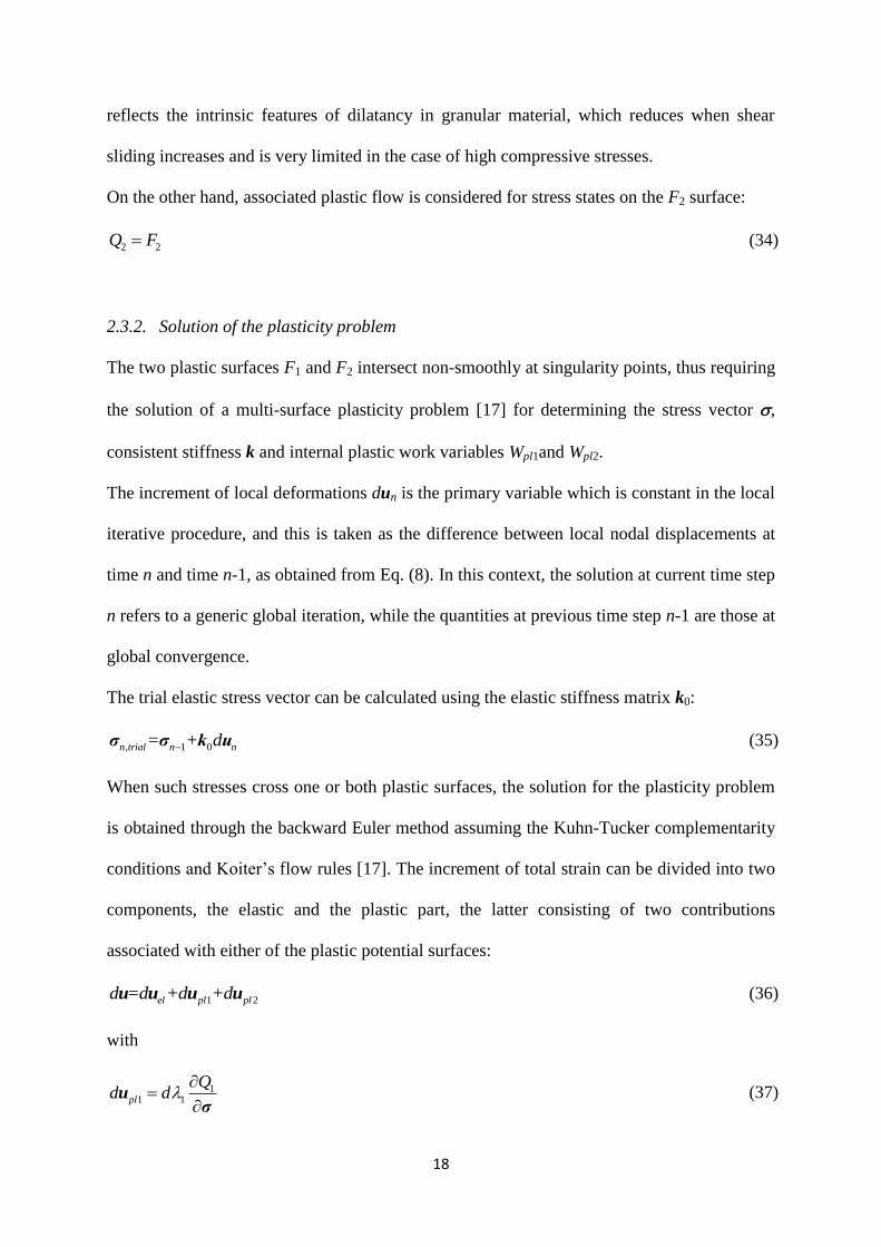
2.3.2. Solution of the plasticity problem

The two plastic surfaces F1 and F2 intersect non-smoothly at singularity points, thus requiring

the solution of a multi-surface plasticity problem [17] for determining the stress vector ,

consistent stiffness k and internal plastic work variables Wpl1and Wpl2.

The increment of local deformations dun is the primary variable which is constant in the local

iterative procedure, and this is taken as the difference between local nodal displacements at

time n and time n-1, as obtained from Eq. (8). In this context, the solution at current time step

n refers to a generic global iteration, while the quantities at previous time step n-1 are those at

global convergence.

The trial elastic stress vector can be calculated using the elastic stiffness matrix k0:

, 1 0n trial n n= + dσ σ k u (35)

When such stresses cross one or both plastic surfaces, the solution for the plasticity problem

is obtained through the backward Euler method assuming the Kuhn-Tucker complementarity

conditions and Koiter’s flow rules [17]. The increment of total strain can be divided into two

components, the elastic and the plastic part, the latter consisting of two contributions

associated with either of the plastic potential surfaces:

1 2el pl pld =d +d +du u u u (36)

with

11 1pl

Qd d

u

σ (37)

19

22 2pl

Qd d

u

σ (38)

where d and dare the increments of the plastic multipliers for the F1 and F2 surfaces,

respectively.

The solution is obtained by considering the loading/unloading conditions [17]:

0id ; , 0i pliF W σ ; , 0i i plid F W σ with i=1,2 (39)

The procedure used by Caballero et al. [24] for smooth plasticity criteria has been employed

and extended to the case of multi-surface plasticity. The plastic multiplier calculation is

integrated with the fracture work and the incremental traction-deformation computation. A

local Newton-Raphson strategy is employed, where the local system of nonlinear equations is

solved using a monolithic iteration technique with sub-stepping. The procedure is based on an

elastic predictor and on a corrector stress based on fracture energy.

Three different cases can occur as shown in Figure 7: the trial stress vector can cross either

F1, F2 or both surfaces. In the following, the procedure employed for the last case, which is

the most general, is detailed.

The stress vector, plastic work variables and plastic multipliers can be determined by solving

the nonlinear system of equations in residual form:

1,

2,

1

1

1 2, 1 0 1, 2,

1, 1, 1, 1, 1, 1

2, 2, 2, 2, 2, 1

, , 1 1,

, , 2 2,

0

, , 0

, , 0

, 0

, 0

pl n

pl n

n n n n n n

n n

W pl n pl n pl n n pl n

W pl n pl n pl n n pl n

F n i n pl n

F n i n pl n

Q Qd d d

R W dW W d W

R W dW W d W

R F W

R F W

σR = σ σ k u

σ σ

σ

σ

σ

σ

(40)

where n-1 and Wpl1,n-1 Wpl2,n-1 are the stresses and plastic work variables at convergence in the

previous time (pseudo-time) step, dWpl1,n and dWpl2,n are the increments of plastic work

variables for the current step n, and n, Wpl1,n, Wpl2,n l1,n andl2,n are the unknowns to be

20

determined. According to the full Netwon-Raphson procedure, the system in Eq. (40) is

linearised leading to:

, 1 , 1 2 1 2, ,0

T

n i n i pl pln i n id dW dW d d R R J σ

(41)

thus:

1

1 2 1 2 ,,,

T

pl pl n in in id dW dW d d

σ J R

(42)

where:

1 2 1 2,,pl pl

T

n i W dW d dn i

R R R R σR R (43)

2

12 23 0 1 2

1 2 1 20 1 0 2 0 02

1 220 2 2

1 1 1

1 1

,2 2 2

2 2

1 1

1

2 1

1

1 0 0

0 1 0

0 0 0

0 0 0

pl pl

pl pl pl

pl

n ipl pl pl

pl

pl

pl

Qd

Q Q Q Qd d

W WQd

dW dW dW

W

dW dW dW

W

F F

W

F F

W

I kσ

k k k kσ σ σ σ

kσ

σ

J

σ

σ

σ,

n i

(44)

in which I3 represents the 3 by 3 identity matrix in the stress space.

The local solution at time step n for global iteration k can be found simply by iterative

correction of the variables until convergence, as defined in terms of the norm of the residuals

being less than a tolerance :

1 1 1

2 2 2

1 1 1

2 2 21 ,

pl pl pl

pl pl pl

j

n n n j

d

W W dW

W W dW

d

d

σ σ σ

with j increased until , ,n i n i R R (45)

21

At the end of the iterative process, the local tangent stiffness kn, consistent with the numerical

solution procedure, is obtained as the first derivative of the stresses with respect to the strains:

n

n

σk

u (46)

This can be determined by linearising the nonlinear equations for the stress components,

included in Rn, whereby the Jacobian Jn, obtained at convergence for the current global

iteration, is employed to determine kn [27]:

-1

0

T

n nk P J Pk (47)

where P corresponds to the projection matrix on the stress space:

3 3 4

T

P I 0 , I3 is a 3×3

identity matrix, and 03×4 is a 3×4 null matrix.

To enhance the robustness of the local solution procedure, a substepping strategy is employed

so that a solution can be found even for relatively large increments of local strains dun. When

the number of iterations required to solve Eq. (40) is greater than a prescribed value nmax1, the

substepping procedure is activated and the total increment of local strains dun, as determined

from the increment of global displacements, is divided into m local substeps [27]:

,n k k nd du u with 1

1m

k

k

and 0 1k k=1..m (48)

An adaptive multi-level substepping strategy is employed, where the step reduction

coefficient k depends on a prescribed constant factor 1 and on the substepping level n

according to 1 n

k When the number of iterations required for a substep k at level n is

greater than nmax1, the level is increased and the reduction coefficient is reduced to

11 n

k . Conversely, if the local solution is successfully found for consecutive substeps,

the substep level is reduced and the reduction coefficient for the following substep is

increased to 1

1 1 n

k

. The procedure stops when 1

1m

k

k

or when the total number of

22

local iterations, the sum of the iterations required at each substep, is greater than a prescribed

maximum value nmax2. In the former case, the local solution for the total increment of local

strains dun, is determined, while in the latter case, step reduction at the global structural level

may be required. As far as the local solution is concerned, at each substep the trial elastic

stress is first obtained, and the activation of either or both plastic surfaces is subsequently

checked, as in the case of monolithic calculation without substeps. If at substep k a plastic

surface is crossed and the solution is found, in the following steps the solution is sought

either along the same surface or at singularity points, where the two surfaces intersect each

other.

At each substep k the stress vector, the plastic work variables and plastic multipliers are

solved for using Eq. (40), where dun is substituted by dun,k, and then transferred to the next

step, until a solution is obtained for the last substep which corresponds to the full increment

dun. Finally, the consistent stiffness matrix is determined by adding the different

contributions from each substep, following the approach proposed in [24] aimed at preserving

quadratic convergence. This process involves differentiating the equations in (40), written for

a substep k, with respect to dun:

1 21, 1 / 2, 1 /

/ 1 /

1, 1 / 1, 1 / 1, 1 / 1, 1 /

2, 1 / 2, 1 / 2, 1 / 2, 1 /

1 1 / 1, 1 /

2 1

, ,

, ,

,

n-1+k/m n k m n k mn k m n k m

pl n k m pl n k m pl n k m n k m

pl n k m pl n k m pl n k m n k mn

n k m pl n k m

n

Q Qd d

W dW W d

W dW W d

F W

F

0σ + k

σ σ

σ

σu

σ

σ

1 ( 1) / ,

1, 1 ( 1) /

2, 1 ( 1) /

/ 2, 1 /

0

0

,

n k m n k

pl n k m

pl n k m

n

k m pl n k m

d

W

W

W

0σ k u

u(49)

At the first substep k=1, 1 0n

n

u,

1, 10

pl n

n

W

u,

2, 10

pl n

n

W

u and the stiffness matrix can be

determined using Eq. (47) applying the chain rule of differentiation:

1-1 1/ -1 1/ 1 1/1 1 1/ 0

1 1/

n m n m n mn m

n n m n

Tσ σ uP J Pk

u u u. (50)

23

For a subsequent generic subincrement 2 k m the contribution from the previous substeps

has to be taken into account [24] leading to:

-1 ( 1) /

0

1, -1 ( 1) /

1-1 /1 /

2, -1 ( 1) /

2,3

n k m

k

n

pl n k m

Tn k mnn k m

n

pl n k m

n

W

W

ku

u= P Ju

u

0

(51)

where the consistent stiffness matrix kn is obtained from Eq. (50) as the final matrix

corresponding to k=m.

In the analyses carried out employing the proposed mesoscale model with nonlinear

interfaces, the use of substepping is found particularly effective when cracks develop along

brick interfaces, principally due to the high elastic stiffness which lead to trial stresses that

are relatively far from the plastic surfaces.

3. Numerical Examples

The proposed nonlinear interface element has been implemented in ADAPTIC [28], a general

finite element code for nonlinear analysis of structures under extreme static and dynamic

loading, which is used here to demonstrate the accuracy and effectiveness of proposed

mesoscale modelling approach for brick-masonry. Numerical results are compared hereafter

with outcomes of experimental tests on URM panels, where both the in-plane and out-of-

plane responses of URM elements are investigated.

3.1. In-Plane Response

Some of the results obtained by Vermeltfoort & Raijmakers [29] in shear tests on single-leaf

panels are considered here for experimental-numerical comparisons. Two solid brick-

24

masonry walls are analysed, which correspond to the identical wall specimens J4D and J5D

and to specimen J7D in [29].

In the tests, all the walls were first preloaded with a vertical top pressure, pv=0.3 MPa for J4D

and J5D and pv=2.12 MPa for J7D, and a horizontal load Fh was then applied in the plane of

the walls at the top edge under displacement control up to collapse (Fig. 8a). The three URM

panels have a width-height ratio of around 1 (990×1000 mm2), and they all feature 18 brick

layers of which only 16 were loaded, and the remaining 2 were fixed to steel beams so as to

keep the top and bottom edges of the element straight during the test. Each brick unit is

204×98×50 mm3, while the bed and head mortar joints are 12.5 mm thick.

During the tests, some horizontal cracks first appeared at the top and bottom of the walls, and

then cracks started developing diagonally, along the bed and head mortar joints and through

the bricks, up to failure. The experimental response was characterized by a softening branch

which started when diagonal cracks suddenly appeared in the centre of the specimens.

The walls are modelled here using the mesoscale approach detailed in previous sections.

Numerical problems occurred when performing static analyses with standard displacement

control techniques [16] especially for the case of higher normal pressure, which were caused

by a sudden release of elastic energy in bulk material when cracks spread along interfaces. In

order to determine the solution up to collapse, a dynamic analysis procedure is utilised,

allowing the sudden release of elastic energy to be balanced by kinetic and viscous energy. In

all analyses, a fixed value of velocity v=0.1 mm/s is applied at all the nodes at the top of the

wall. Moreover prescribed vertical displacements are applied at the same nodes to reproduce

the effect of the vertical pressure pv, and all the displacements at the bottom are fully

restrained to represent a fixed support. Finally, zero acceleration is assigned to the top nodes

during the analysis to ensure a linear variation with time of the top wall displacements.

25

Tables 2 and 3 show the mechanical properties for brick and brick-mortar interfaces

employed in the analyses. These values, mainly determined from tests on single masonry

components (units and mortar), were reported in previous research [9,23,26]. Moreover,

regarding the clay bricks, an elastic modulus Eb=16700 MPa and a Poisson ratio b=0.15 are

assumed [9,26], while a density b=19∙10-9

Ns2/mm

4 and mass-proportional damping,

corresponding to a damping ratio =5%, are used for the solid elements to represent inertia

and damping effects.

In order to evaluate the performance of the proposed mesoscale model for brick-masonry, the

results obtained from different meshes have been compared. In 3D nonlinear models, the use

of a fine mesh could become prohibitively expensive; therefore, the choice of the coarsest

possible mesh that achieves acceptable accuracy is fundamental in order to reduce the

computational effort in detailed modelling of URM structures. Two different meshes have

been considered and compared in the analyses, as shown in Figure 8b. For the coarser mesh

(mesh 1), only one 20-noded solid element is used per half brick, such that two interface

elements are employed for each bed joints with only one interface element for each head joint

and for modelling potential vertical cracks at the mid-plane of the bricks (brick-brick

interface). In the finer mesh (mesh 2), each half unit is modelled using four solid elements,

thus corresponding to a refinement of mesh 1 where the number of elements along the x and z

directions is doubled. Therefore, four interfaces are used for each bed joint, and two

interfaces are employed for each head joint and at the mid-plane of each brick unit.

The influence of the number of Gauss points in the nonlinear interface has also been

investigated, so as to establish whether increasing the number of integration points leads to

improved solution accuracy as a substitute for mesh refinement. Figure 9 provides

experimental-numerical comparisons, where the experimental load-displacement curves for

J4D, J5D and J7D walls are compared with the numerical results determined using the

26

coarser mesh (mesh 1) and 7x7 Gauss points for integration over the interface elements. In

this figure, the numerical predictions reported by Lourenço & Rots [9] and calculated using

planar elements (4×2 8-noded 2D elements for each brick) and nonlinear line interfaces are

also shown. A good agreement between experimental and numerical results can be observed

up to collapse, including initial stiffness, maximum capacity and the post-peak response of

the walls. The predicted response is smooth for walls J4D and J5D subject to the lower

vertical load pv, while it exhibits jumps in the steep softening branch for wall J7D. The

predictions of the proposed modelling approach are generally close to those reported in [9]

for all walls, with the current predictions of the post-peak response for wall J7D evidently

better.

Figure 10 depicts the influence of both mesh refinement and the number of Gauss points used

for the interface elements. The results obtained using mesh 1 and mesh 2 are compared,

where two different curves are shown for the coarser mesh, obtained respectively using 3×3

and 7×7 Gauss points, while only 3×3 Gauss point are employed for mesh 2. The predictions

of mesh 1 with the larger number of integration points are coincident with those of mesh 2,

while the predictions of mesh1 with 3×3 Gauss points exhibit some minor discrepancies in

comparison. These outcomes show that the use of an increased number of integration points

(super-integration) for interface elements provides smooth and accurate results, very close to

those achieved through mesh refinement. This is particularly important since integration

refinement is much less computationally demanding than mesh refinement.

The employment of super-integration for the interface is particularly effective since the 3D

solid elements, representing bricks, generally have a much higher stiffness than damage

interfaces. Therefore, these 3D elements behave as rigid blocks, thus the change in the

interface displacement field upon mesh refinement is negligible.

27

Finally, Figure 11 shows the deformed shape, and the interface plastic work contours at

collapse, which are compared to the crack paths surveyed in the tests for walls J4D and J5D.

The results shown are those from mesh 1 with 7×7 Gauss points, where the plastic work Wpl1

associated with the F1 plastic surface assumes maximum values close to the fracture energies

Gf,II along the diagonal direction of the wall, while plastic work Wpl2 associated with F2

assumes high values close to the crushing energy Gc in the compressed bed joints at the two

edges of the wall. These predictions are in good agreement with the main crack paths and

with the results reported in [9].

3.2. Out-of-plane response

Numerical analyses are also carried out to establish the effectiveness of the developed

mesoscale modelling approach for investigating the out-of-plane behaviour of URM walls,

where comparisons are made against the experiments performed by Bean Popehn et al. [30]

and Chee Liang [31].

Bean Popehn et al. [30] carried out experiments to investigate the buckling behaviour of

slender URM walls subject to vertical and out-of-plane lateral loads. The static response of a

clay brick-masonry panel 3.26 m high and 0.803 m wide with a thickness of 89.9 mm

(specimen B1-25 in [30]) is considered here, where the brick units are 89.9×57.2×193.7 mm3

and the joints are 10 mm thick. The wall, supported against out-of-plane displacements at the

two horizontal edges, is firstly loaded by a vertical force Pv=111 kN, which is followed by an

out-of-plane horizontal force Fh using a whittletree arrangement with spreader beams that

allowed a close representation of a uniform load distribution. The lateral supports did not

represent perfect simple supports, thus providing some resistance to the wall rotation.

Accoridngly, an effective height of the wall was established as 2.41 m, measuring the

distance between the two points of inflection. In the test, the wall exhibited linear behaviour

28

until some horizontal cracks occurred in the bed joints around mid-height, then increasing the

lateral load, a single large horizontal crack developed when the maximum wall capacity was

reached. The test continued under displacement control in order to assess the post-peak

behaviour.

While mechanical properties for the components (units, mortar) were not reported [30], some

average properties for masonry assumed as a continuum material (i.e. flexural tensile strength

mt=0.372 MPa) were provided. In previous research [12], it was shown that the collapse

mechanism of walls loaded out-of-plane is different from that of URM elements loaded in-

plane, because it is determined mainly by the tensile instead of the shear response. Therefore,

the tensile strength t0 and the Mode-I fracture energy Gf;I for mortar joints are the key

parameters in advanced mesoscale models for studying the out-of-plane capacity and the

post-peak response of URM walls.

As suggested in [12], t0 can be calculated from mt, which is obtained in physical tests on

the assumption of an elastic response, considering a uniform plastic distribution of tensile

stresses over the interface and fixing the centre of rotation at the external edge of the masonry

panel cross section. Thus the simple relation t0 =1/3∙mt has been employed in the current

analyses. Moreover, in assessing the behaviour of slender walls under vertical loads when

flexural buckling is a potential cause of failure, other fundamental parameters to be

accurately determined are the elastic modulus of bricks and mortar joints. Since these values

were also not reported [30], the elastic stiffness for brick and mortar has been calibrated so as

to allow good correlation against the initial wall stiffness as observed in the tests.

Table 4 provides the mechanical properties used for the nonlinear interfaces, while an elastic

modulus Eb=10000 MPa and a Poisson ratio b=0.15 are assumed for bricks. In the performed

analyses, according to the description of the test setup and the observed experimental

behaviour [30], the initial load Pv is applied considering an eccentricity equal to 7 mm to

29

represent initial imperfections, while a uniform distribution of nodal forces is used to

represent the variable out-of-plane horizontal loads.

The wall has been represented as a simply supported structure, considering the effective

height and using the coarsest mesh allowable in the proposed modelling approach, utilising

only one solid element for half a unit. Different numbers of Gauss points are also considered

to establish whether increasing the number of integration points leads to improved accuracy

as in the analysis of walls loaded in-plane. All the predictions are obtained using static

analysis with standard arc-length displacement control [16].

Figure 12 compares the experimental load deflection response with that predicted using 3×3,

7×7 and 10×10 Gauss points for interface elements. The results achieved confirm the

effectiveness of using a high number of integration points, which provide smooth and

accurate results. More importantly, a comparison is made in Figure 12 between the

predictions accounting for and neglecting geometric nonlinearity, including large

displacements. These results demonstrate the importance of accounting for geometric

nonlinearity in the mesoscale model for masonry, as it clearly enables a more accurate

prediction of the actual behaviour of slender walls. Neglecting geometric nonlinearity leads

to a significant inaccuracy for walls loaded by vertical and horizontal actions, where the

strength is typically determined by out-of-plane instability. Furthermore, the consideration of

geometric nonlinearity is essential for modelling the buckling response of masonry panels

under vertical loading. As shown in Figure 13, which depicts the buckling response under

vertical load Pv for wall B1-25 are shown, the consideration of geometric nonlinearity

assuming linear material behaviour enables the elastic buckling load to be obtained.

Obviously, a purely linear wall response would be obtained for the same case ignoring

geometric nonlinearity. Furthermore, the same figure shows the added influence of material

30

nonlinearity for the considered wall, which is shown in this case to affect only the post-peak

behaviour.

In the final comparison, the out-of-plane behaviour of a solid wall, simply supported along its

four edges and subjected to bi-axial bending, is considered, where reference is made to

experiments undertaken by Chee Liang [31] on two identical specimens wall 8 and wall 12.

The single-leaf URM panel is 1190 mm high, 795 mm wide and 53 mm thick, comprising

112x53x36 mm3 bricks and 10 mm thick mortar joints. The two specimens were loaded up to

collapse by applying a uniform out-of-plane pressure through an air-bag sandwiched between

the wall and a stiff reacting frame. Another stiff steel frame was connected to wall on the

other side, so as to prevent out-of-plane displacements and provide fixed supports along the

four edges. Tests were also performed on components, where the compressive strength of

mortar, the tensile and compressive strength of bricks and the flexural strength of masonry

were determined. As mentioned above, the out-of-plane capacity of the wall is strongly

influenced by the tensile strength of the masonry joints, and its actual initial stiffness is

affected by both the brick and mortar elastic modulus. These values were not determined

experimentally [31]; therefore, the same procedure described before for relating the mortar

tensile strength to the masonry flexural resistance is used. Table 5 provides the material

parameters used for the interfaces elements, which correspond to the values used in [12] for

the same wall, while the elastic stiffness of brick and mortar are assumed the same as in [13].

Figure 14 provides the numerical-experimental comparisons, where one 20-noded solid

element is used for each half brick and 3×3 Gauss points for each interface element. The

experimental results reported in [31] for wall 8 and wall 12 correspond to a partial load-

displacement curve for wall 8 and the maximum capacity for both walls, where the

displacement in the figure is at the centre of the wall. Good agreement can be observed

between the numerical and experimental results. Using the material parameters for the

31

interfaces as suggested in [12], a maximum lateral pressure for the wall, very close to the

experimental capacity and to the collapse pressure determined in [12] through a 3D limit

analysis approach, is established. Unlike limit analysis, however, the proposed modelling

approach enables the prediction of the initial stiffness and the post-peak response of the wall

loaded out-of-plane. Finally, Figure 15 shows the deformed shape at collapse, which is

compared with the actual crack pattern. The large vertical crack which runs along the head

mortar joints and bricks as well as the continuous diagonal cracks observed in the tests are

well represented using the proposed mesoscale model with nonlinear interface elements.

4. Conclusion

This paper presents a nonlinear interface element which is incorporated into a mesoscale

model for nonlinear analysis of URM structures. The proposed mesoscale approach considers

a detailed description for the 3D arrangement that characterises the texture of walls in URM

buildings. Compared to previous mesoscale models for brick-masonry, the proposed

approach accounts for both geometric and material nonlinearity and is based on the use of 2D

nonlinear interface elements along with 3D solid elements, allowing the simulation of both

the in-plane and out-of-plane response of URM walls.

A co-rotational formulation is adopted to account for geometric nonlinearity, including large

displacement effects, and a work-softening non-associated plasticity approach, utilising a

multi-surface plasticity criterion, is employed for the force-displacement material law at the

interfaces.

The results of numerical analyses carried out to investigate both the in-plane and the out-of-

plane response of brick-masonry panels up to collapse are presented, where comparisons are

made against experimental outcomes. It is shown that the use of the proposed nonlinear 2D

interface elements with 3D brick elements allows the consideration of both initial and

32

damage-induced anisotropy of brick-masonry. The main features of the structural behaviour,

including initial stiffness, maximum capacity and post-peak response, are also accurately

determined. In performing numerical simulations, the mesh density and the number of Gauss

points for the interface elements are varied so as to establish the coarsest mesh that can still

achieve reasonable accuracy in detailed nonlinear analysis of URM structures. It is shown

that the use of only one 20-noded 3D element per half brick with the associated 2D interface

elements provides good accuracy for both in-plane and out-of-plane nonlinear analysis, and

that increasing the number of Gauss points can substitute for mesh refinement in achieving

improved accuracy.

The results achieved demonstrate the significant potential of the proposed approach. The

detailed mesoscale model with nonlinear interfaces, while potentially associated with

significant computational demands, can be incorporated into a full multiscale approach in

which the accurate mesoscale description and the structural scale are fully coupled, thus

allowing the nonlinear analysis of larger scale structures [14]. This is an area of research that

is currently being pursued by the authors.

Acknowledgement

The authors gratefully acknowledge the support provided for this research by the 7th

European Community Framework Programme through a Marie Curie Intra-European

Fellowship (Grant Agreement Number: PIEF-GA-2008-220336).

References

1. Goodman RE, Taylor RL, Brekke T. A model for the mechanics of jointed rock, J. Soil

Mech. Found. Div. Proc. ASCE 1968; 94, SM 3:637-659.

33

2. Rots JG. Computational modeling of concrete structures, PhD Thesis, Delft University of

Technology, 1988.

3. Alfano G, Crisfield MA. Finite element interface models for delamination analysis of

laminated composites: mechanical and computational issues, Int. J. Numer. Methods

Engrg 2001; 50:1701-1736.

4. Seguarado J, LLorca J. A new three-dimensional interface finite element to simulate

fracture in composites, Int. J Solids and Struct. 2004; 41:2977-2993.

5. Brocks W, Cornec A, Scheider I. Computational Aspects of Nonlinear Fracture

Mechanics; In: I. Milne, R. O. Ritchie, B. Karihaloo (Eds.): Comprehensive Structural

Integrity - Numerical and Computational Methods 2003. Vol. 3, Oxford: Elsevier, 127-

209.

6. Carol I, Lopez CM, Roa O. Micromechanical analysis of quasi-brittle materials using

fracture-based interface elements, Int. J. Numer. Methods Engrg 2001; 52:193-215.

7. Alfano G, Sacco E. Combining interface damage and friction in cohesive-zone model,

Int. J. Numer. Methods Engrg 2006; 68:542-582.

8. Dhanasekar M, Page AW, Kleeman PW. The failure of brick masonry under biaxial

stresses, Proc. Instn. Civ. Eng. 1985; 79, 2: 295-313.

9. Lourenço PB, Rots JG. Multisurface Interface Model for Analysis of Masonry

Structures, . J. Engrg. Mech. ASCE 1997; 123, 7:660-668.

10. Gambarotta L, Lagomarsino S. Damage models for the seismic response of brick

masonry shear walls. Part I: the mortar joint model and its applications, Earthquake Eng.

Struct. Dynam. 1997; 26:423-439.

11. Shien-Beygi B, Pietruszczak S. Numerical analysis of structural masonry: mesoscale

approach, Computer and Struct. 2008; 86:1958-1973.

34

12. Milani G. 3D upper bond limit analysis of multi-leaf masonry walls, Int. J. Mechanical

Sciences 2008; 50:817-836.

13. Griffith MC, Lam NTK., Wilson JL, Doherty K. Experimental investigation of

unreinforced brick masonry walls in flexure, J. Struct. Engrg. ASCE 2004; 130, 3:423-

431.

14. Massart TJ, Peerlings RHJ, Geers MGD. An enhanced multi-scale approach for masonry

wall computations with localizations of damage, Int. J. Numer. Meth. Engng 2007;

69:1022-1059.

15. Chaboche JL, Feyel F, Monerie Y. Interface debonding models: a viscous regularization

with a limited rate dependency, Int. J. Solid and Structures 2001; 38:3127-3160.

16. Cristfield MA. Non-linear Finite Element Analysis of Solids and Structures. Vol. 1:

Essential. John Wiley and Sons, 1997, Chichester, UK.

17. Simo JC, Hughes TJR. Computational Inelasticity: vol. 7 Interdisciplinary Applied

Mathematics 1998, Springer, New York.

18. Zienkiewicz OC, Taylor RL. The finite element method. Vol. 1: The Basis. Fifth edition

2000. Butterworth-Heinemann.

19. Zienkiewicz OC, Taylor RL. The finite element method. Vol. 1: Solid Mechanics. Fifth

edition 2000. Butterworth-Heinemann.

20. Izzuddin BA. An enhanced co-rotational approach for large displacement analysis of

plates, Int. J. Numer. Meth. Engrg 2005; 64:1350-1374.

21. Schellekens JCJ, de Borst R. On the numerical integration of interface elements, Int. J.

Numer. Meth. Engrg 1993; 36:43-66.

22. Point N, Sacco E. A delamination model for laminate composites. Int. J Solids and

Struct. 1996; 33(4):483-509.

35

23. Chaimoon K, Attard MM. Modelling of unreinforced masonry wall under shear and

compression, Comp. and Struct. 2007; 29:2056-2068.

24. Caballero A, Willam KJ, Carol I. Consistent tangent formulation for 3D interface

modelling of cracking/fracture in quasi-brittle materials, Comput. Methods Appl. Mech.

Engrg. 2008; 197:2804-2822.

25. Hilsdorf HK. Investigation into the failure mechanism of brick masonry loaded in axial

compression. In: Proceeding of designing, engineering and construction with Masonry

products. Houston, USA, Gulf publishing company 1969; 34-14.

26. Rots JG. (Ed). Structural Masonry: An Experimental/Numerical Basis for Practical

Design Rules, A.A. Balkema 1997, Rotterdam, the Netherlands.

27. Pérez-Foguet A, Rodriguez-Ferran A, Huerta A. Consistent tangent matrices for

substepping schemes, Comput. Methods Appl. Mech. Engrg. 2000; 190:4627-4647.

28. Izzuddin BA. Nonlinear Dynamic Analysis of Framed Structures, PhD Thesis, Imperial

College, 1991.

29. Vermeltfoort AT, Raijmakers TMJ. Deformation controlled meso shear tests on masonry

piers – Part.2, Draft Report, TU Eindhoven, dept. BKO, 1993.

30. Bean Popehn JR., Shultz AE, Lu M., Stolarski HK, Ojard NJ. Influence of transverse

loading on the stability of slender unreinforced masonry walls, Engrg Struct. 2008;

30:2830-2839.

31. Chee Liang NG. Experimental and theoretical investigation of the behavior of brickwork

cladding panel subjected to lateral loading, PhD Thesis, University of Edinburgh, 1996.

36

Table 1. Initial values and primary variables for material parameters.

F1, Q1 F2, Q2

C, CQ t tantanQ D c tanθ

Evolution law Eq. (28) Eq. (28) Eq. (29) Eq. (28) Eq. (29) Eq. (29)

Initial

parameters and

variables

A=C, CQ

A0=C0, CQ0

W*=Wpl1

G*=Gf,II

A=t

A0=t0

W*=Wpl1

G*=Gf,I

B=tantanQ

B0=tan0tanQ

Br=tanrtanQr

W*=Wpl1

G*=Gf,I

A=D

A0=D0

W*=Wpl2

G*=Gc

B=c

B0=c0

Br=cr

W*=Wpl2

G*=Gc

B=tan

B0=tan0

Br=tanr

W*=Wpl2

G*=Gc

Table 2. Mechanical properties of nonlinear interface elements for J4D/J5D walls [29].

Elastic properties Surface F1 Surface Q1 Surfaces F2, Q2

Mortar

kn = 82 N/mm3

kt = 36 N/mm3

t0 =0.25 MPa

C0 =0.375 MPa

tan0

tan

Gf,I =0.018 N/mm

Gf,II =0.125 N/mm

t0 =0.25 MPa

C0 =37.5 MPa

tan0

tan

c0 =10.5 MPa

cr =1.5 MPa

D =10.5 MPa

tan0

tan0

Gc = 5.0 N/mm

Brick

kn = 1.0∙104N/mm

3

kt = 1.0∙104N/mm

3

t0 =2.0 MPa

C0 =2.8 MPa

tan0

tan

Gf,I =0.08 N/mm

Gf,II =0.5 N/mm

t0 =2.0 MPa

C0 =2.8 MPa

tan0

tan

Gf,I =0.08 N/mm

Gf,II =0.5 N/mm

Table 3. Mechanical properties of nonlinear interface elements for J7D wall [29].

Elastic properties Surface F1 Surface Q1 Surfaces F2, Q2

Mortar

kn = 82 N/mm3

kt = 36 N/mm3

t0 =0.16 MPa

C0 =0.224 MPa

tan0

tan

Gf,I =0.018 N/mm

Gf,II =0.05 N/mm

t0 =0.16 MPa

C0 =22.4 MPa

tan0

tan

c0 =11.5 MPa

cr =1.5 MPa

D =11.5 MPa

tan0

tan0

Gc = 5.0 N/mm

Brick

kn = 1.0∙104N/mm

3

kt = 1.0∙104N/mm

3

t0 =2.0 MPa

C0 =2.8 MPa

tan0

tan

Gf,I =0.08 N/mm

Gf,II =0.5 N/mm

t0 =2.0 MPa

C0 =2.8 MPa

tan0

tan

Gf,I =0.08 N/mm

Gf,II =0.5 N/mm

37

Table 4. Mechanical properties of nonlinear interface elements for B1-25 wall [30].

Elastic properties Surface F1 Surface Q1 Surfaces F2, Q2

Mortar

kn = 120 N/mm3

kt = 80 N/mm3

t0 =0.124 MPa

C0 =0.21 MPa

tan0

tan

Gf,I =0.02 N/mm -

N/mm

Gf,II =0.05 N/mm

t0 =0.124 MPa

C0 =0.21 MPa

tan0

tan

c0 =32.5 MPa

cr =0.0 MPa

D = 10.0 MPa

tan0

tan0

Gc = 5.0 N/mm

Brick

kn = 1.0∙104N/mm

3

kt = 1.0∙104N/mm

3

t0 =2.0 MPa

C0 =2.8 MPa

tan0

tan

Gf,I =0.08 N/mm

Gf,I =0.5 N/mm

t0 =2.0 MPa

C0 =2.8 MPa

tan0

tan

Table 5. Mechanical properties of nonlinear interface elements for wall tested by Chee Liang

et al. [31].

Elastic properties Surface F1 Surface Q1 Surfaces F2, Q2

Mortar

kn = 250 N/mm3

kt = 105 N/mm3

t0 =0.35 MPa

C0 =0.42 MPa

tan0

tan

Gf,I =0.018 N/mm -

0.036 N/mm

Gf,II =0.125 N/mm

t0 =0.35 MPa

C0 =42.0 MPa

tan0

tan

c0 =6.0 MPa

cr =0.0 MPa

D = 6.0 MPa

tan0

tan0

Gc = 5.0 N/mm

Brick

kn = 1.0∙104N/mm

3

kt = 1.0∙104N/mm

3

t0 =1.0 MPa

C0 =1.2 MPa

tan0

tan

Gf,I =0.08 N/mm

Gf,I =0.5 N/mm

t0 =1.0 MPa

C0 =1.2 MPa

tan0

tan

38

List of figures

Figure 1. Interface elements for modelling brick-masonry.

Figure 2. 3D mesoscale modelling for brick-masonry with 20-noded solid elements and 2D

nonlinear interfaces.

Figure 3. Solution procedure for the mesoscale modelling approach.

Figure 4. Global and local co-rotational systems.

Figure 5. (a) Initial plastic surfaces and potentials, (b) evolution of plastic surfaces.

Figure 6. Traction deformation response: (a) tension, (b) shear.

Figure 7. Solution procedure for the local plasticity problem at quadrature point level.

Figure 8. URM wall loaded in plane: (a) boundary conditions [29], (b) employed meshes.

Figure 9. Experimental-numerical comparisons for the URM wall loaded in plane.

Figure 10. Numerical comparisons for the wall loaded in-plane: influence of mesh

refinement and integration points.

Figure 11. Wall loaded in-plane: (a) deformed shape (displacement scale=20) and (b) plastic

work contours at collapse, (c) cracks paths surveyed after the tests [29].

Figure 12. Experimental-numerical comparison for the URM wall B1-25 loaded out-of-

plane.

Figure 13. Buckling load for the URM wall B1-25.

Figure 14. Wall loaded out-of-plane [30]: numerical-experimental comparisons.

Figure 15. Wall loaded out-of-plane : (a) deformed shape (displacement scale=100) and (b)

plastic work contours at the end of the analysis, (c) cracks paths surveyed after the test [30].

39

Figure 1. Interface elements for modelling brick-masonry.

40

Figure 2. 3D mesoscale modelling for brick-masonry with 20-noded solid elements and 2D

nonlinear interfaces.

41

Figure 3. Solution procedure for the mesoscale modelling approach.

42

Figure 4. Global and local co-rotational systems.

43

(a)

(b)

Figure 5. (a) Initial plastic surfaces and potentials, (b) evolution of plastic surfaces.

44

(a)

(b)

Figure 6. Traction deformation response: (a) tension, (b) shear.

45

Figure 7. Solution procedure for the local plasticity problem at quadrature point level.

46

Figure 8. URM wall loaded in plane: (a) boundary conditions [29], (b) employed meshes.

47

Figure 9. Experimental-numerical comparisons for the URM wall loaded in plane.

48

Figure 10. Numerical comparisons for the wall loaded in-plane: influence of mesh

refinement and integration points.

49

Figure 11. Wall loaded in-plane: (a) deformed shape (displacement scale=20) and (b) plastic

work contours at collapse, (c) cracks paths surveyed after the tests [29].

50

Figure 12. Experimental-numerical comparison for the URM wall B1-25 loaded out-of-

plane.

51

Figure 13. Buckling load for the URM wall B1-25.

52

Figure 14. Wall loaded out-of-plane [30]: numerical-experimental comparisons.

53

Figure 15. Wall loaded out-of-plane : (a) deformed shape (displacement scale=100) and (b)

plastic work contours at the end of the analysis, (c) cracks paths surveyed after the test [30].