A Non-Destructive Evaluation Application Using Software ...
148
Air Force Institute of Technology Air Force Institute of Technology AFIT Scholar AFIT Scholar Theses and Dissertations Student Graduate Works 3-26-2020 A Non-Destructive Evaluation Application Using Software Defined A Non-Destructive Evaluation Application Using Software Defined Radios and Bandwidth Expansion Radios and Bandwidth Expansion Nicholas J. O'Brien Follow this and additional works at: https://scholar.afit.edu/etd Part of the Electrical and Electronics Commons Recommended Citation Recommended Citation O'Brien, Nicholas J., "A Non-Destructive Evaluation Application Using Software Defined Radios and Bandwidth Expansion" (2020). Theses and Dissertations. 3186. https://scholar.afit.edu/etd/3186 This Thesis is brought to you for free and open access by the Student Graduate Works at AFIT Scholar. It has been accepted for inclusion in Theses and Dissertations by an authorized administrator of AFIT Scholar. For more information, please contact richard.mansfield@afit.edu.
Transcript of A Non-Destructive Evaluation Application Using Software ...

Air Force Institute of Technology Air Force Institute of Technology
AFIT Scholar AFIT Scholar
Theses and Dissertations Student Graduate Works
3-26-2020
A Non-Destructive Evaluation Application Using Software Defined A Non-Destructive Evaluation Application Using Software Defined
Radios and Bandwidth Expansion Radios and Bandwidth Expansion
Nicholas J. O'Brien
Follow this and additional works at: https://scholar.afit.edu/etd
Part of the Electrical and Electronics Commons
Recommended Citation Recommended Citation O'Brien, Nicholas J., "A Non-Destructive Evaluation Application Using Software Defined Radios and Bandwidth Expansion" (2020). Theses and Dissertations. 3186. https://scholar.afit.edu/etd/3186
This Thesis is brought to you for free and open access by the Student Graduate Works at AFIT Scholar. It has been accepted for inclusion in Theses and Dissertations by an authorized administrator of AFIT Scholar. For more information, please contact [email protected].
A NON-DESTRUCTIVE EVALUATIONAPPLICATION USING SOFTWARE
DEFINED RADIOS AND BANDWIDTHEXPANSION
THESIS
Nicholas J O’Brien, Flight Lieutenant, RAAF
AFIT-ENG-MS-20-M-049
DEPARTMENT OF THE AIR FORCEAIR UNIVERSITY
AIR FORCE INSTITUTE OF TECHNOLOGY
Wright-Patterson Air Force Base, Ohio
DISTRIBUTION STATEMENT AAPPROVED FOR PUBLIC RELEASE; DISTRIBUTION UNLIMITED.

The views expressed in this document are those of the author and do not reflect theofficial policy or position of the United States Air Force, the United States Departmentof Defense or the United States Government. This material is declared a work of theU.S. Government and is not subject to copyright protection in the United States.

AFIT-ENG-MS-20-M-049
A NON-DESTRUCTIVE EVALUATION APPLICATION USING SOFTWARE
DEFINED RADIOS AND BANDWIDTH EXPANSION
THESIS
Presented to the Faculty
Department of Electrical and Computer Engineering
Graduate School of Engineering and Management
Air Force Institute of Technology
Air University
Air Education and Training Command
in Partial Fulfillment of the Requirements for the
Degree of Master of Science in Electrical Engineering
Nicholas J O’Brien, BENG (Electrical and Electronic)
Flight Lieutenant, RAAF
March 26,2020
DISTRIBUTION STATEMENT AAPPROVED FOR PUBLIC RELEASE; DISTRIBUTION UNLIMITED.
AFIT-ENG-MS-20-M-049
A NON-DESTRUCTIVE EVALUATION APPLICATION USING SOFTWARE
DEFINED RADIOS AND BANDWIDTH EXPANSION
THESIS
Nicholas J O’Brien, BENG (Electrical and Electronic)Flight Lieutenant, RAAF
Committee Membership:
Dr. Peter J. CollinsChair
Dr. Michael A. TempleMember
Major J. Addison Betances, Ph.DMember
AFIT-ENG-MS-20-M-049
Abstract
The development of low-complexity, lightweight and low-cost Non-Destructive
Evaluation (NDE) equipment for microwave device testing is desirable from a main-
tenance efficiency and operational availability perspective. Current NDE equipment
tends to be custom-designed, cumbersome and expensive. Software Defined Radio
(SDR) technology, and a bandwidth expansion technique that exploits a priori trans-
mit signal knowledge and auto-correlation provides a solution.
This research investigated the reconstruction of simultaneous SDR receiver in-
stantaneous bandwidth (sub-band) collections using single, dual and multiple SDR
receivers. The adjacent sub-bands, collectively spanning a transmit signal bandwidth
were auto-correlated with a replica transmit signal to restore frequency and phase
offsets. The offsets arise due to different local oscillator manufacturing tolerances,
temperature effects and ageing.
A 100 MHz bandwidth uniform white noise signal was reconstructed from both
dual (2× 50 MHz) and multiple (4× 25 MHz) SDR collections. The 100 MHz band-
width exceeds a B205 SDR receiver instantaneous bandwidth. The auto-correlation
technique minimizes SDR hardware numbers as bandwidth overlap is not required.
Hardware test Symbol Error Rate (SER) was compared with a theoretical coher-
ently detected M-ary orthogonal signal. A 2 MHz dual SDR uniform white noise
signal reconstruction exhibited a 5 dBW loss when compared with the theoretical
value. The 4 MHz multiple SDR signal reconstruction exhibited a 6 dBW loss.
Finally, a linear feedback shift register was used to generate the uniform white
noise signal. This provided near true-noise characteristics employing a polynomial
primitive to ensure 236 − 1 non-repeatable sequences.
iv

Acknowledgements
I would like to thank my beautiful wife for taking care of everything so I could
devote time to my studies. Beyond the shadow of a doubt, your encouragement and
support got me through the tougher days.
To my advisor Dr. P. Collins, committee members, instructors, staff and students
who steered me through the obstacles on the way you have my gratitude. I enjoyed
having a ‘yarn’ whenever the opportunity arose. You are all great people.
Dr. M. Temple, Capt. Y. Matsui and Capt. N. Echeverry deserve a special men-
tion, thanks for the RF-DNA signal collection conversion code, the Ubuntu assistance,
and the Frequency Locked Loop assisted Phase Locked Loop conceptual discussion.
Finally, I am especially indebted to two AFIT members; Maj. J.A. Betances,
Ph.D and Mr Michael Paprocki. Maj. Betances for the countless hours you invested
in ensuring I graduated. More so than most research efforts, this thesis document
is attributable to your mentoring, enthusiasm and endless patience, as well as being
the prime contributor to auto-correlation code development. Mr Michael Paprocki
(IMSO) for being just a phone call away from the moment we touched down in the
USA. It was reassuring to have such a genuine person in your position, not to mention
that you tell the best stories. You are both ‘Top Blokes’.
Nicholas J O’Brien
v

Table of Contents
Page
Abstract . . . . . . . . . . . . . . . . . . . . . . . . . . . . . . . . . . . . . . . . . . . . . . . . . . . . . . . . . . . . . . . iv
Acknowledgements . . . . . . . . . . . . . . . . . . . . . . . . . . . . . . . . . . . . . . . . . . . . . . . . . . . . . . . v
List of Figures . . . . . . . . . . . . . . . . . . . . . . . . . . . . . . . . . . . . . . . . . . . . . . . . . . . . . . . . . viii
List of Tables . . . . . . . . . . . . . . . . . . . . . . . . . . . . . . . . . . . . . . . . . . . . . . . . . . . . . . . . . . xiii
List of Acronyms . . . . . . . . . . . . . . . . . . . . . . . . . . . . . . . . . . . . . . . . . . . . . . . . . . . . . . . xiv
I. Introduction . . . . . . . . . . . . . . . . . . . . . . . . . . . . . . . . . . . . . . . . . . . . . . . . . . . . . . . . 1
1.1 Background . . . . . . . . . . . . . . . . . . . . . . . . . . . . . . . . . . . . . . . . . . . . . . . . . . . . 11.2 Problem Statement . . . . . . . . . . . . . . . . . . . . . . . . . . . . . . . . . . . . . . . . . . . . . . 21.3 Research Objectives . . . . . . . . . . . . . . . . . . . . . . . . . . . . . . . . . . . . . . . . . . . . . 41.4 Research Implications . . . . . . . . . . . . . . . . . . . . . . . . . . . . . . . . . . . . . . . . . . . . 51.5 Summary . . . . . . . . . . . . . . . . . . . . . . . . . . . . . . . . . . . . . . . . . . . . . . . . . . . . . . 6
II. Literature Review . . . . . . . . . . . . . . . . . . . . . . . . . . . . . . . . . . . . . . . . . . . . . . . . . . . 7
2.1 Non-Destructive Evaluation . . . . . . . . . . . . . . . . . . . . . . . . . . . . . . . . . . . . . . . 72.2 Software Defined Radio . . . . . . . . . . . . . . . . . . . . . . . . . . . . . . . . . . . . . . . . . . 9
2.2.1 Ettus USRP B205-mini Software Defined Radio . . . . . . . . . . . . . . 102.2.2 Ettus USRP X310 Software Defined Radio . . . . . . . . . . . . . . . . . . . 102.2.3 GNU Radio Companion Interface Software . . . . . . . . . . . . . . . . . . . 12
2.3 Bandwidth Expansion Principles . . . . . . . . . . . . . . . . . . . . . . . . . . . . . . . . . 182.3.1 Wide Sense Stationary Measurement Techniques . . . . . . . . . . . . . . 192.3.2 Wide Sense Stationary Reference Techniques . . . . . . . . . . . . . . . . . 242.3.3 Non-Wide Sense Stationary Techniques . . . . . . . . . . . . . . . . . . . . . . 27
2.4 Device Classification . . . . . . . . . . . . . . . . . . . . . . . . . . . . . . . . . . . . . . . . . . . . 352.4.1 Signal Selection . . . . . . . . . . . . . . . . . . . . . . . . . . . . . . . . . . . . . . . . . . 352.4.2 Signal Collection . . . . . . . . . . . . . . . . . . . . . . . . . . . . . . . . . . . . . . . . . 372.4.3 Fingerprint Generation . . . . . . . . . . . . . . . . . . . . . . . . . . . . . . . . . . . . 372.4.4 Device Training and Classification . . . . . . . . . . . . . . . . . . . . . . . . . . 38
2.5 Summary . . . . . . . . . . . . . . . . . . . . . . . . . . . . . . . . . . . . . . . . . . . . . . . . . . . . . 41
III. Methodology . . . . . . . . . . . . . . . . . . . . . . . . . . . . . . . . . . . . . . . . . . . . . . . . . . . . . . 42
3.1 Bandwidth Expansion Modelling . . . . . . . . . . . . . . . . . . . . . . . . . . . . . . . . . 433.1.1 The Communications System Signal Process
Model . . . . . . . . . . . . . . . . . . . . . . . . . . . . . . . . . . . . . . . . . . . . . . . . . . 433.1.2 Signal Generation and Processing . . . . . . . . . . . . . . . . . . . . . . . . . . . 473.1.3 Signal Process Model Validation . . . . . . . . . . . . . . . . . . . . . . . . . . . . 55
vi

Page
3.1.4 Symbol Recovery Measurement . . . . . . . . . . . . . . . . . . . . . . . . . . . . . 563.2 Bandwidth Expansion Techniques . . . . . . . . . . . . . . . . . . . . . . . . . . . . . . . . 57
3.2.1 Auto-correlation - Frequency ‘Pull-In’ . . . . . . . . . . . . . . . . . . . . . . . 583.2.2 Auto-correlation - Phase Correction . . . . . . . . . . . . . . . . . . . . . . . . . 603.2.3 Transmit Signal Preparation . . . . . . . . . . . . . . . . . . . . . . . . . . . . . . . 60
3.3 Bandwidth Expansion Application . . . . . . . . . . . . . . . . . . . . . . . . . . . . . . . . 633.3.1 Single Receiver Dual Channel Simulations . . . . . . . . . . . . . . . . . . . 643.3.2 Dual Receiver Simulations . . . . . . . . . . . . . . . . . . . . . . . . . . . . . . . . . 653.3.3 Multiple Receiver Simulations . . . . . . . . . . . . . . . . . . . . . . . . . . . . . . 663.3.4 Single Receiver Hardware Tests . . . . . . . . . . . . . . . . . . . . . . . . . . . . . 663.3.5 Dual Receiver Hardware Tests . . . . . . . . . . . . . . . . . . . . . . . . . . . . . . 693.3.6 Multiple Receiver Hardware Tests . . . . . . . . . . . . . . . . . . . . . . . . . . 72
3.4 Scaling the Bandwidth Expansion Technique . . . . . . . . . . . . . . . . . . . . . . . 763.5 RFDNA Test Case . . . . . . . . . . . . . . . . . . . . . . . . . . . . . . . . . . . . . . . . . . . . . 783.6 Summary . . . . . . . . . . . . . . . . . . . . . . . . . . . . . . . . . . . . . . . . . . . . . . . . . . . . . 79
IV. Results and Analysis . . . . . . . . . . . . . . . . . . . . . . . . . . . . . . . . . . . . . . . . . . . . . . . . 80
4.1 Validation Results . . . . . . . . . . . . . . . . . . . . . . . . . . . . . . . . . . . . . . . . . . . . . . 804.2 Simulation Results . . . . . . . . . . . . . . . . . . . . . . . . . . . . . . . . . . . . . . . . . . . . . 82
4.2.1 Dual Receiver Simulations . . . . . . . . . . . . . . . . . . . . . . . . . . . . . . . . . 824.2.2 Multiple Receiver Simulations . . . . . . . . . . . . . . . . . . . . . . . . . . . . . . 89
4.3 Hardware Test Results . . . . . . . . . . . . . . . . . . . . . . . . . . . . . . . . . . . . . . . . . . 934.3.1 Single Receiver Hardware Test Results . . . . . . . . . . . . . . . . . . . . . . 934.3.2 Dual Receiver Hardware Test Results . . . . . . . . . . . . . . . . . . . . . . . 994.3.3 Multiple Receiver Hardware Test Results . . . . . . . . . . . . . . . . . . . 106
4.4 RFDNA Test Results . . . . . . . . . . . . . . . . . . . . . . . . . . . . . . . . . . . . . . . . . . 1134.5 Summary . . . . . . . . . . . . . . . . . . . . . . . . . . . . . . . . . . . . . . . . . . . . . . . . . . . . 113
V. Conclusion . . . . . . . . . . . . . . . . . . . . . . . . . . . . . . . . . . . . . . . . . . . . . . . . . . . . . . . 115
5.1 Future Work . . . . . . . . . . . . . . . . . . . . . . . . . . . . . . . . . . . . . . . . . . . . . . . . . . 1175.1.1 Bandwidth Expansion Technique Transfer . . . . . . . . . . . . . . . . . . 1175.1.2 Alternate Support Hardware Tests . . . . . . . . . . . . . . . . . . . . . . . . . 1175.1.3 SDR Filter Attenuation . . . . . . . . . . . . . . . . . . . . . . . . . . . . . . . . . . 1185.1.4 RF-DNA Tests . . . . . . . . . . . . . . . . . . . . . . . . . . . . . . . . . . . . . . . . . . 118
Appendix A: Non-Linear Least Squares Estimation. . . . . . . . . . . . . . . . . . . . . . . . . . . . . . . . . . . . . . . . . . . . . . . . . . . . . . . . . 119Appendix B: Simulation Summary. . . . . . . . . . . . . . . . . . . . . . . . . . . . . . . . . . . . . . . . . . . . . . . . . . . . . . . . . 123Appendix C: Hardware Test Summary. . . . . . . . . . . . . . . . . . . . . . . . . . . . . . . . . . . . . . . . . . . . . . . . . . . . . . . . . 124Bibliography . . . . . . . . . . . . . . . . . . . . . . . . . . . . . . . . . . . . . . . . . . . . . . . . . . . . . . . . . . 125
vii
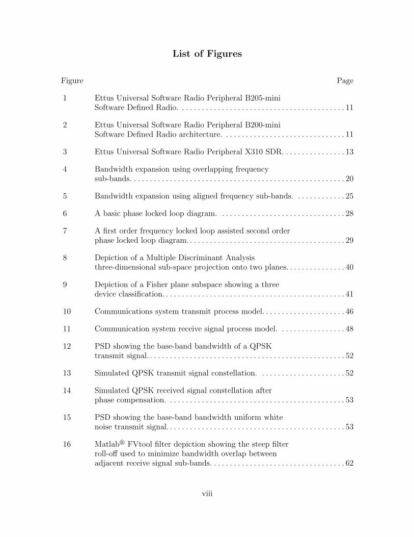
List of Figures
Figure Page
1 Ettus Universal Software Radio Peripheral B205-miniSoftware Defined Radio. . . . . . . . . . . . . . . . . . . . . . . . . . . . . . . . . . . . . . . . . . 11
2 Ettus Universal Software Radio Peripheral B200-miniSoftware Defined Radio architecture. . . . . . . . . . . . . . . . . . . . . . . . . . . . . . . 11
3 Ettus Universal Software Radio Peripheral X310 SDR. . . . . . . . . . . . . . . . 13
4 Bandwidth expansion using overlapping frequencysub-bands. . . . . . . . . . . . . . . . . . . . . . . . . . . . . . . . . . . . . . . . . . . . . . . . . . . . . . 20
5 Bandwidth expansion using aligned frequency sub-bands. . . . . . . . . . . . . 25
6 A basic phase locked loop diagram. . . . . . . . . . . . . . . . . . . . . . . . . . . . . . . . 28
7 A first order frequency locked loop assisted second orderphase locked loop diagram. . . . . . . . . . . . . . . . . . . . . . . . . . . . . . . . . . . . . . . . 29
8 Depiction of a Multiple Discriminant Analysisthree-dimensional sub-space projection onto two planes. . . . . . . . . . . . . . . 40
9 Depiction of a Fisher plane subspace showing a threedevice classification. . . . . . . . . . . . . . . . . . . . . . . . . . . . . . . . . . . . . . . . . . . . . . 41
10 Communications system transmit process model. . . . . . . . . . . . . . . . . . . . . 46
11 Communication system receive signal process model. . . . . . . . . . . . . . . . . 48
12 PSD showing the base-band bandwidth of a QPSKtransmit signal. . . . . . . . . . . . . . . . . . . . . . . . . . . . . . . . . . . . . . . . . . . . . . . . . . 52
13 Simulated QPSK transmit signal constellation. . . . . . . . . . . . . . . . . . . . . . 52
14 Simulated QPSK received signal constellation afterphase compensation. . . . . . . . . . . . . . . . . . . . . . . . . . . . . . . . . . . . . . . . . . . . . 53
15 PSD showing the base-band bandwidth uniform whitenoise transmit signal. . . . . . . . . . . . . . . . . . . . . . . . . . . . . . . . . . . . . . . . . . . . . 53
16 Matlabr FVtool filter depiction showing the steep filterroll-off used to minimize bandwidth overlap betweenadjacent receive signal sub-bands. . . . . . . . . . . . . . . . . . . . . . . . . . . . . . . . . . 62
viii

Figure Page
17 Filtered 1 MHz uniform white noise signal sub-band fortransmit signal construction. . . . . . . . . . . . . . . . . . . . . . . . . . . . . . . . . . . . . . 62
18 Hardware circuit setup for single SDR receiver tests. . . . . . . . . . . . . . . . . . 69
19 GNU radio companion interface setup for single SDRhardware tests. . . . . . . . . . . . . . . . . . . . . . . . . . . . . . . . . . . . . . . . . . . . . . . . . . 70
20 Hardware circuit setup for dual SDR receiver tests. . . . . . . . . . . . . . . . . . . 72
21 GNU radio companion interface setup for dual SDRreceiver hardware tests. . . . . . . . . . . . . . . . . . . . . . . . . . . . . . . . . . . . . . . . . . . 73
22 Hardware circuit setup for multiple SDR receiver test. . . . . . . . . . . . . . . . 74
23 GNU radio companion interface setup for multiple SDRreceiver hardware test. . . . . . . . . . . . . . . . . . . . . . . . . . . . . . . . . . . . . . . . . . . 75
24 Monte Carlo simulation for the QPSK signal systemprocess model validation showing SER versus Es/N0 forthe single receiver, dual channel case. . . . . . . . . . . . . . . . . . . . . . . . . . . . . . . 81
25 Monte Carlo simulation for the uniform white noisesignal system process model validation showing SERversus Es/N0 for the single receiver, dual channel case. . . . . . . . . . . . . . . . 81
26 Simulated 2 MHz uniform white noise transmit andreceive signal frequency pull in correlation sequence fora dual SDR collection. . . . . . . . . . . . . . . . . . . . . . . . . . . . . . . . . . . . . . . . . . . . 84
27 Simulated 2 MHz uniform white noise transmit signalPSD for dual SDR collection. . . . . . . . . . . . . . . . . . . . . . . . . . . . . . . . . . . . . . 85
28 Simulated 2 MHz uniform white noise overlay signalPSD showing the two 1 MHz SDR collections. . . . . . . . . . . . . . . . . . . . . . . 85
29 Simulated 2 MHz uniform white noise recombined signalPSD for a dual SDR collection. . . . . . . . . . . . . . . . . . . . . . . . . . . . . . . . . . . . 86
30 Simulated 2 MHz uniform white noise transmit andreceive symbol correlation for a dual SDR collectionshowing uncorrected correlation lag. . . . . . . . . . . . . . . . . . . . . . . . . . . . . . . . 87
ix
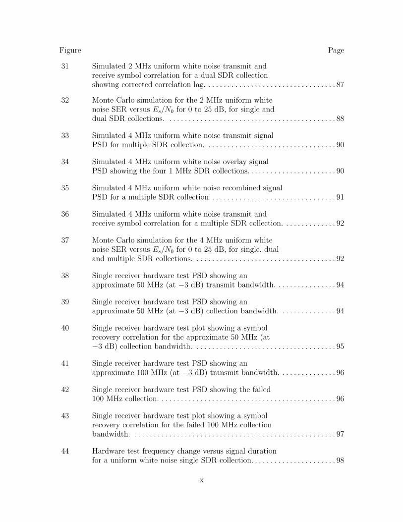
Figure Page
31 Simulated 2 MHz uniform white noise transmit andreceive symbol correlation for a dual SDR collectionshowing corrected correlation lag. . . . . . . . . . . . . . . . . . . . . . . . . . . . . . . . . . 87
32 Monte Carlo simulation for the 2 MHz uniform whitenoise SER versus Es/N0 for 0 to 25 dB, for single anddual SDR collections. . . . . . . . . . . . . . . . . . . . . . . . . . . . . . . . . . . . . . . . . . . . 88
33 Simulated 4 MHz uniform white noise transmit signalPSD for multiple SDR collection. . . . . . . . . . . . . . . . . . . . . . . . . . . . . . . . . . 90
34 Simulated 4 MHz uniform white noise overlay signalPSD showing the four 1 MHz SDR collections. . . . . . . . . . . . . . . . . . . . . . . 90
35 Simulated 4 MHz uniform white noise recombined signalPSD for a multiple SDR collection. . . . . . . . . . . . . . . . . . . . . . . . . . . . . . . . . 91
36 Simulated 4 MHz uniform white noise transmit andreceive symbol correlation for a multiple SDR collection. . . . . . . . . . . . . . 92
37 Monte Carlo simulation for the 4 MHz uniform whitenoise SER versus Es/N0 for 0 to 25 dB, for single, dualand multiple SDR collections. . . . . . . . . . . . . . . . . . . . . . . . . . . . . . . . . . . . . 92
38 Single receiver hardware test PSD showing anapproximate 50 MHz (at −3 dB) transmit bandwidth. . . . . . . . . . . . . . . . 94
39 Single receiver hardware test PSD showing anapproximate 50 MHz (at −3 dB) collection bandwidth. . . . . . . . . . . . . . . 94
40 Single receiver hardware test plot showing a symbolrecovery correlation for the approximate 50 MHz (at−3 dB) collection bandwidth. . . . . . . . . . . . . . . . . . . . . . . . . . . . . . . . . . . . . 95
41 Single receiver hardware test PSD showing anapproximate 100 MHz (at −3 dB) transmit bandwidth. . . . . . . . . . . . . . . 96
42 Single receiver hardware test PSD showing the failed100 MHz collection. . . . . . . . . . . . . . . . . . . . . . . . . . . . . . . . . . . . . . . . . . . . . . 96
43 Single receiver hardware test plot showing a symbolrecovery correlation for the failed 100 MHz collectionbandwidth. . . . . . . . . . . . . . . . . . . . . . . . . . . . . . . . . . . . . . . . . . . . . . . . . . . . . 97
44 Hardware test frequency change versus signal durationfor a uniform white noise single SDR collection. . . . . . . . . . . . . . . . . . . . . . 98
x

Figure Page
45 Hardware test 2 MHz uniform white noise transmitsignal PSD for dual SDR collection. . . . . . . . . . . . . . . . . . . . . . . . . . . . . . . 101
46 Hardware test 2 MHz uniform white noise overlay signalPSD showing the two 1 MHz SDR collections. . . . . . . . . . . . . . . . . . . . . . 101
47 Hardware test 2 MHz uniform white noise recombinedsignal PSD for a dual SDR collection. . . . . . . . . . . . . . . . . . . . . . . . . . . . . 102
48 Hardware test 2 MHz uniform white noise transmit andreceive symbol correlation for a dual SDR collection. . . . . . . . . . . . . . . . 102
49 Hardware test 2 MHz uniform white noise SER versusEs/N0 for 0 to 25 dB, for a dual SDR collection. . . . . . . . . . . . . . . . . . . . 103
50 Hardware test 20 MHz uniform white noise overlaysignal PSD showing the two 10 MHz SDR collections. . . . . . . . . . . . . . . 104
51 Hardware test 100 MHz uniform white noise overlaysignal PSD showing the two 50 MHz SDR collections. . . . . . . . . . . . . . . 104
52 Hardware test 100 MHz uniform white noise transmitand receive symbol correlation for a dual SDR collection. . . . . . . . . . . . . 105
53 Hardware test 4 MHz uniform white noise transmitsignal PSD for multiple SDR collection. . . . . . . . . . . . . . . . . . . . . . . . . . . . 107
54 Hardware test 4 MHz uniform white noise overlay signalPSD showing the four 1 MHz SDR collections. . . . . . . . . . . . . . . . . . . . . . 108
55 Hardware test 4 MHz uniform white noise recombinedsignal PSD for a multiple SDR collection. . . . . . . . . . . . . . . . . . . . . . . . . . 108
56 Hardware test 4 MHz QPSK overlay signal for amultiple SDR collection. . . . . . . . . . . . . . . . . . . . . . . . . . . . . . . . . . . . . . . . . 109
57 Hardware test 4 MHz QPSK overlay signal showing thefour 1 MHz SDR collections. . . . . . . . . . . . . . . . . . . . . . . . . . . . . . . . . . . . . 109
58 Hardware test 4 MHz uniform white noise transmit andreceive symbol correlation for a multiple SDR collection. . . . . . . . . . . . . 111
59 Hardware test 4 MHz uniform white noise SER versusEs/N0 for 0 to 25 dB, for a multiple SDR collection. . . . . . . . . . . . . . . . . 111
xi
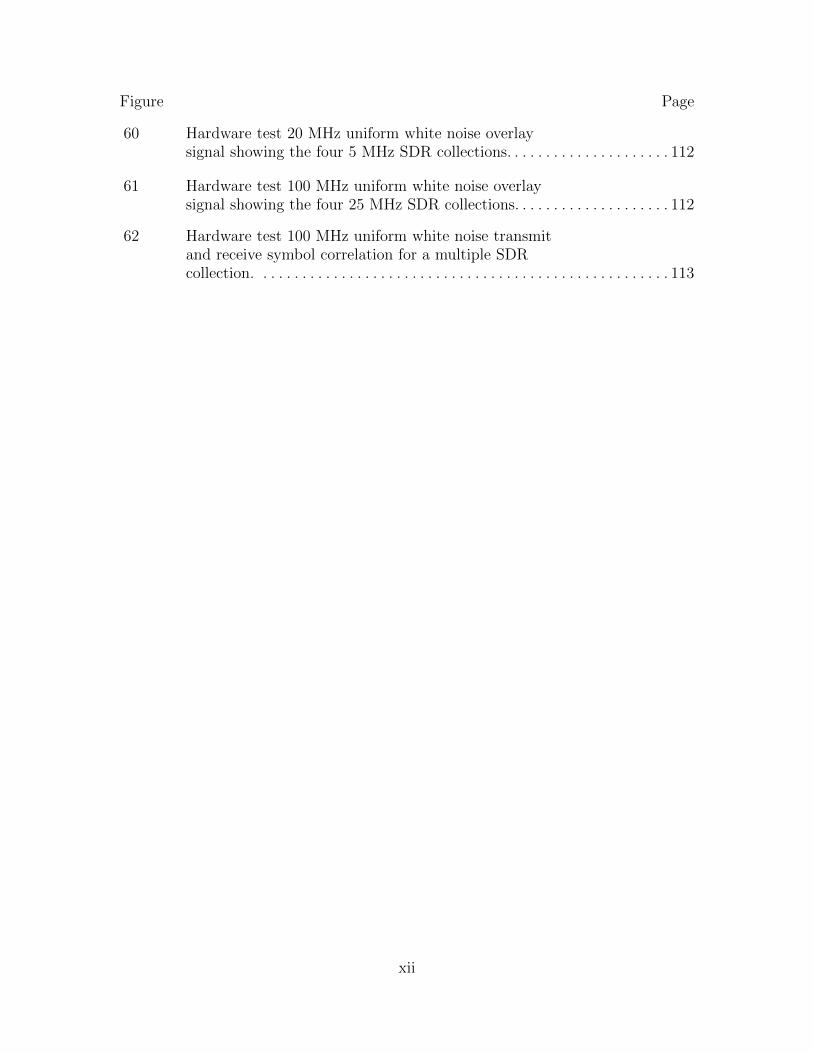
Figure Page
60 Hardware test 20 MHz uniform white noise overlaysignal showing the four 5 MHz SDR collections. . . . . . . . . . . . . . . . . . . . . 112
61 Hardware test 100 MHz uniform white noise overlaysignal showing the four 25 MHz SDR collections. . . . . . . . . . . . . . . . . . . . 112
62 Hardware test 100 MHz uniform white noise transmitand receive symbol correlation for a multiple SDRcollection. . . . . . . . . . . . . . . . . . . . . . . . . . . . . . . . . . . . . . . . . . . . . . . . . . . . . 113
xii
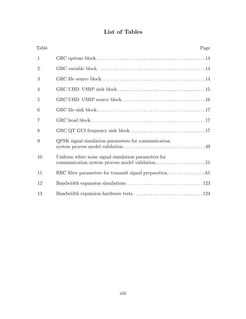
List of Tables
Table Page
1 GRC options block. . . . . . . . . . . . . . . . . . . . . . . . . . . . . . . . . . . . . . . . . . . . . . 14
2 GRC variable block. . . . . . . . . . . . . . . . . . . . . . . . . . . . . . . . . . . . . . . . . . . . . 14
3 GRC file source block. . . . . . . . . . . . . . . . . . . . . . . . . . . . . . . . . . . . . . . . . . . . 14
4 GRC UHD: USRP sink block. . . . . . . . . . . . . . . . . . . . . . . . . . . . . . . . . . . . . 15
5 GRC UHD: USRP source block. . . . . . . . . . . . . . . . . . . . . . . . . . . . . . . . . . . 16
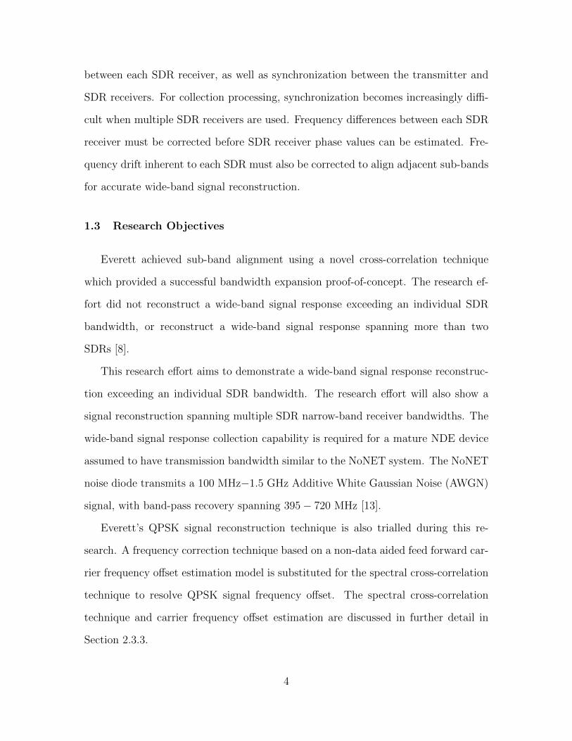
6 GRC file sink block. . . . . . . . . . . . . . . . . . . . . . . . . . . . . . . . . . . . . . . . . . . . . . 17
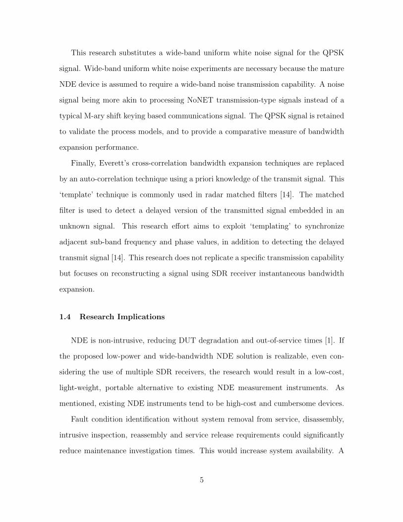
7 GRC head block. . . . . . . . . . . . . . . . . . . . . . . . . . . . . . . . . . . . . . . . . . . . . . . . 17
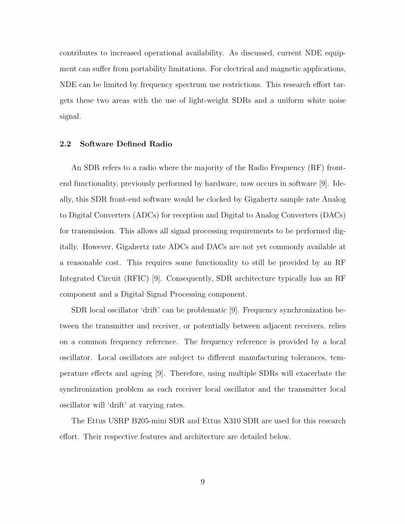
8 GRC QT GUI frequency sink block. . . . . . . . . . . . . . . . . . . . . . . . . . . . . . . . 17
9 QPSK signal simulation parameters for communicationsystem process model validation. . . . . . . . . . . . . . . . . . . . . . . . . . . . . . . . . . . 49
10 Uniform white noise signal simulation parameters forcommunication system process model validation. . . . . . . . . . . . . . . . . . . . . 51
11 RRC filter parameters for transmit signal preparation. . . . . . . . . . . . . . . . 61
12 Bandwidth expansion simulations. . . . . . . . . . . . . . . . . . . . . . . . . . . . . . . . 123
13 Bandwidth expansion hardware tests. . . . . . . . . . . . . . . . . . . . . . . . . . . . . 124
xiii
List of Acronyms
10G ETH 10 Gigabit Ethernet.
1G ETH 1 Gigabit Ethernet.
ADC Analog to Digital Converter.
AFIT Air Force Institute of Technology.
AWG Analog Waveform Generator.
AWGN Additive White Gaussian Noise.
BER Bit Error Rate.
DAC Digital to Analog Converter.
DFT Discrete Fourier Transform.
DUT Device Under Test.
FIR Finite Impulse Response.
FLD Fisher Linear Discriminant.
FLL Frequency Locked Loop.
FPGA Field Programmable Gate Array.
FSK Frequency Shift Keying.
GPS Global Positioning System.
GPSDO Global Positioning System Disciplined Oscillator.
xiv
GRC GNU Radio Companion.
GUI Graphic User Interface.
IDFT Inverse Discrete Fourier Transform.
ISI Inter-Symbol Interference.
LFSR Linear Feed-back Shift Register.
LPI Low Probability of Intercept.
Matlabr Matrix Laboratory.
MDA Multiple Discriminant Analysis.
MLE Maximum Likelihood Estimation.
NDE Non-Destructive Evaluation.
NDT Non-Destructive Testing.
NLS Non-Linear Least Squares.
NoNET Noise Radar Network.
OQPSK Offset-Quadrature Phase Shift Keying.
PLL Phase Locked Loop.
PMF Probability Mass Function.
PPS Pulse Per Second.
PSD Power Spectral Density.
xv
QPSK Quadrature Phase Shift Keying.
RF Radio Frequency.
RF-DNA Radio Frequency-Distinct Native Attribute.
RFIC RF Integrated Circuit.
RRC Raised Root Cosine.
SDR Software Defined Radio.
SER Symbol Error Rate.
SMA Sub-Minature Version A.
SNR Signal-to-Noise Ratio.
SURE Stimulated Unintended Radiated Emissions.
USRP Universal Software Radio Peripheral.
VCO Voltage Controlled Oscillator.
WSS Wide Sense Stationary.
xvi

A NON-DESTRUCTIVE EVALUATION APPLICATION USING SOFTWARE
DEFINED RADIOS AND BANDWIDTH EXPANSION
I. Introduction
1.1 Background
Competing operational availability and system-maintenance demands are common
in today’s defense environment where budgetary constraints and high costs can limit
the use of redundant systems. Non-Destructive Evaluation (NDE) offers a poten-
tial solution providing Device Under Test (DUT) system maintenance measurement
without impairing serviceability [1]. Instrument portability, complexity and cost can
limit NDE adoption with some technicians preferring intrusive practices such as Bit
Error Rate Testing or Time Domain Reflectometry. Frequency spectrum regulation
and Radio Frequency Interference can also constrain adoption when testing involves
electrical measurements [2].
Recent research efforts combine Air Force Institute of Technology (AFIT) Noise
Radar Network (NoNET), Stimulated Unintended Radiated Emissions (SURE) and
Radio Frequency-Distinct Native Attribute (RF-DNA) techniques to characterize the
behaviour of microwave devices [2–7]. The devices are stimulated with an active noise
interrogation signal. The successful noise signal experiments demonstrated concurrent
frequency spectrum use with other Radio Frequency (RF) sources [4]. The non-
intrusive characteristics of the measurement system show promising results for the
field of NDE [7]. However, the NoNET system is not portable.
As early as 1959, McMaster acknowledged that portability was a primary factor
1

in NDE (then Non-Destructive Testing (NDT)) adoption [1]. Recent AFIT research
investigated the portability, complexity and cost issues surrounding the SURE process
and NoNET. This research applied a non-Wide Sense Stationary (WSS) bandwidth
expansion technique to reconstruct a Quadrature Phase Shift Keying (QPSK) signal.
The technique restored a 1.98 MHz bandwidth using two Software Defined Radio
(SDR) narrow-band (1 MHz) receiver collections [8]. The collections were conducted
simultaneously. The Software Defined Radios provided a light-weight, low-complexity
and low-cost alternative to the previously used NoNET. The bandwidth expansion
technique provided a means for SURE collection and reconstruction of non-WSS
signals.
Further investigation of active noise signal collection using SDR receivers and a re-
liable bandwidth expansion technique is warranted. The non-intrusive characteristics
of the active noise signal, and consequently the NDE device, would be of significant
benefit to maintenance fault investigation.
To exploit NDE characteristics a proposed device would need sufficient instan-
taneous receiver bandwidth to support microwave device, RF front-end, cable and
connector characterization using SURE and RF-DNA processes. The challenge is
to provide sufficient instantaneous receiver bandwidth for accurate wide-band signal
reconstruction.
1.2 Problem Statement
The problem is to collect, and then reconstruct, a wide-band uniform white noise
signal. The transmitted signal bandwidth is assumed to span multiple SDR receiver
bandwidths. The transmit signal is also assumed to be time-variant. Therefore, the
recovery requires multiple SDRs to effect simultaneous collection of the wide-band
signal. Each SDR collecting an allocated part (sub-band) of the signal.
2
The collected sub-bands must then be processed using a non-WSS bandwidth
expansion technique that accounts for the time varying nature of the uniform white
noise signal. The technique must resolve time-alignment, frequency drift and phase
correction issues. This must occur with sufficient accuracy to align SDR sub-band
signals, allowing for transmit symbols to be recovered from the restored signal.
Software Defined Radios typically have a narrow instantaneous bandwidth. Their
light weight, low complexity and low cost enhances portability, flexibility and mar-
ketability. This is at the expense of Analog to Digital Converter (ADC) bit-rate
performance. Low ADC bit-rates limit SDR instantaneous bandwidth [9]. Previ-
ous work identified device characterization is optimized when the DUT is stimulated
with a wide-band signal; that is, wider than the frequency response of the DUT [6].
Therefore, SDR instantaneous bandwidth limitations appear to be inconsistent with
the requirement for wide-band signal response collection.
This presents a challenge. SDRs commonly support Megahertz bandwidths (e.g. Et-
tus Universal Software Radio Peripheral (USRP) B205-mini SDR has a 56 MHz in-
stantaneous bandwidth [10]) while many microwave devices support Gigahertz band-
widths (e.g. Mini-Circuits model ZX60-14012L+ amplifier has a 30 kHz-14 GHz in-
stantaneous bandwidth [6]). This implies a single SDR receiver must collect and store
consecutive wide-band signal portions until all sub-bands are collected for processing.
This is suitable where “a time delay in the input sequence causes [an] equivalent
time delay in the systems output sequence” [11], (i.e. a time-invariant system) and
where the signal statistics are time invariant [12] (i.e. WSS). However, if the wide-
band system is time-variant or signals are non-WSS, then simultaneous collection of
the entire bandwidth using multiple SDRs is required [8].
Assuming the signal response is non-WSS, simultaneous bandwidth collection for
accurate signal reconstruction requires time, frequency and phase synchronization
3
between each SDR receiver, as well as synchronization between the transmitter and
SDR receivers. For collection processing, synchronization becomes increasingly diffi-
cult when multiple SDR receivers are used. Frequency differences between each SDR
receiver must be corrected before SDR receiver phase values can be estimated. Fre-
quency drift inherent to each SDR must also be corrected to align adjacent sub-bands
for accurate wide-band signal reconstruction.
1.3 Research Objectives
Everett achieved sub-band alignment using a novel cross-correlation technique
which provided a successful bandwidth expansion proof-of-concept. The research ef-
fort did not reconstruct a wide-band signal response exceeding an individual SDR
bandwidth, or reconstruct a wide-band signal response spanning more than two
SDRs [8].
This research effort aims to demonstrate a wide-band signal response reconstruc-
tion exceeding an individual SDR bandwidth. The research effort will also show a
signal reconstruction spanning multiple SDR narrow-band receiver bandwidths. The
wide-band signal response collection capability is required for a mature NDE device
assumed to have transmission bandwidth similar to the NoNET system. The NoNET
noise diode transmits a 100 MHz−1.5 GHz Additive White Gaussian Noise (AWGN)
signal, with band-pass recovery spanning 395− 720 MHz [13].
Everett’s QPSK signal reconstruction technique is also trialled during this re-
search. A frequency correction technique based on a non-data aided feed forward car-
rier frequency offset estimation model is substituted for the spectral cross-correlation
technique to resolve QPSK signal frequency offset. The spectral cross-correlation
technique and carrier frequency offset estimation are discussed in further detail in
Section 2.3.3.
4
This research substitutes a wide-band uniform white noise signal for the QPSK
signal. Wide-band uniform white noise experiments are necessary because the mature
NDE device is assumed to require a wide-band noise transmission capability. A noise
signal being more akin to processing NoNET transmission-type signals instead of a
typical M-ary shift keying based communications signal. The QPSK signal is retained
to validate the process models, and to provide a comparative measure of bandwidth
expansion performance.
Finally, Everett’s cross-correlation bandwidth expansion techniques are replaced
by an auto-correlation technique using a priori knowledge of the transmit signal. This
‘template’ technique is commonly used in radar matched filters [14]. The matched
filter is used to detect a delayed version of the transmitted signal embedded in an
unknown signal. This research effort aims to exploit ‘templating’ to synchronize
adjacent sub-band frequency and phase values, in addition to detecting the delayed
transmit signal [14]. This research does not replicate a specific transmission capability
but focuses on reconstructing a signal using SDR receiver instantaneous bandwidth
expansion.
1.4 Research Implications
NDE is non-intrusive, reducing DUT degradation and out-of-service times [1]. If
the proposed low-power and wide-bandwidth NDE solution is realizable, even con-
sidering the use of multiple SDR receivers, the research would result in a low-cost,
light-weight, portable alternative to existing NDE measurement instruments. As
mentioned, existing NDE instruments tend to be high-cost and cumbersome devices.
Fault condition identification without system removal from service, disassembly,
intrusive inspection, reassembly and service release requirements could significantly
reduce maintenance investigation times. This would increase system availability. A
5

recent example is a wireless RF laboratory test for connector continuity. The test
demonstrated the ability to distinguish loose and damaged Sub-Minature Version A
(SMA) and Type N connectors without having to remove the DUT from service [7].
The mature NDE application would benefit the Department of Defense, Australian
Defence Force and wider industry.
1.5 Summary
Chapter I described the need for an NDE device, outlined the research problem,
detailed the research objectives and identified the research implications. This re-
search effort is documented as follows: Chapter II provides the necessary theoretical
background required to prepare the reader for understanding the research being un-
dertaken, including a review of bandwidth expansion research; Chapter III describes
the simulation and test methodologies implemented to trial bandwidth expansion
techniques; Chapter IV details simulation and test results, and provides analysis;
while Chapter V concludes with the research findings and identifies future work.
6

II. Literature Review
The following sections provide the necessary theoretical background and a sum-
mary of current bandwidth expansion research to prepare the reader for this research
effort. Section 2.1 defines Non-Destructive Evaluation (NDE), discusses NDE ben-
efits and identifies NDE applications; Section 2.2 describes Software Defined Radio
(SDR) technology, details Ettus Universal Software Radio Peripheral (USRP) B205-
mini SDR and the Ettus USRP X310 SDR features and architecture. This section
also describes the GNU Radio Companion (GRC) software that provides the inter-
face between the host-PC and the SDRs. The description includes summary tables of
all processing blocks used for this research effort, and their affected parameters. Sec-
tion 2.3 describes bandwidth expansion principles using Wide Sense Stationary (WSS)
and non-WSS research examples. The non-data-aided feed forward carrier frequency
offset estimation model and phase-offset cross-correlation techniques are discussed
here; finally Section 2.4 describes signal collection and the Radio Frequency-Distinct
Native Attribute (RF-DNA) processes used for device classification.
2.1 Non-Destructive Evaluation
McMaster provides a NDE (then Non-Destructive Testing (NDT)) definition.
“The science of nondestructive [evaluation] embraces all methods for the detection
or measurement of the significant properties or performance capabilities of materi-
als, parts, assemblies, equipment or structures, by tests which do not impair their
serviceability,” [1].
NDE is of significant benefit for maintenance servicing. In many cases NDE lim-
its, or removes, the need for traditional maintenance practices where system service
removal, disassembly, inspection, maintenance and repair, reassembly and service
7

release are required. With renewed emphasis on asset management, Device Under
Test (DUT) inspection using non-intrusive processes allows for more frequent mon-
itoring while reducing maintenance down-times. Non-intrusive processes can also
limit service damage. A frequent monitoring regime supports transition from preven-
tative maintenance practices, using time-based assembly replacement, to predictive
practices, whereby assembly replacement occurs on detection or measurement of a
specific event [15].
The scope of NDE application is broad, and includes the measurement of geometric
properties (e.g. thickness), mechanical properties (e.g. hardness), thermal properties
(e.g. heat resistance) and electrical and magnetic properties. Historical electrical and
magnetic property measurement include eddy current tests to check for structural
discontinuities, Megger tests to check the condition of electrical wiring insulation
and conductivity tests to check for dielectric thickness [1]. More recent electrical
and magnetic based NDE applications include antenna acceptance tests [2], amplifier
acceptance tests [6] and connector continuity tests [7].
For this research effort, DUT materials, parts, assemblies, equipment or structures
are selected microwave devices. The detection or measurement method involves DUT
stimulation using the Stimulated Unintended Radiated Emissions (SURE) process, so
as not to impair serviceability. The significant electrical property measurements are
classified using RF-DNA. RF-DNA discriminates signal features. For example, the
feature could discriminate between products to serial number, or the feature could dis-
criminate between a serviceable and unserviceable device (e.g. A functioning antenna
microwave amplifier or a faulty Sub-Minature Version A (SMA) connector) [2–4,6,7].
Further RF-DNA discussion is provided in Section 2.4.
In summary, NDE has the potential to reduce traditional maintenance practice
duration, limit servicing damage and delay assembly replacement requirements which
8
contributes to increased operational availability. As discussed, current NDE equip-
ment can suffer from portability limitations. For electrical and magnetic applications,
NDE can be limited by frequency spectrum use restrictions. This research effort tar-
gets these two areas with the use of light-weight SDRs and a uniform white noise
signal.
2.2 Software Defined Radio
An SDR refers to a radio where the majority of the Radio Frequency (RF) front-
end functionality, previously performed by hardware, now occurs in software [9]. Ide-
ally, this SDR front-end software would be clocked by Gigahertz sample rate Analog
to Digital Converters (ADCs) for reception and Digital to Analog Converters (DACs)
for transmission. This allows all signal processing requirements to be performed dig-
itally. However, Gigahertz rate ADCs and DACs are not yet commonly available at
a reasonable cost. This requires some functionality to still be provided by an RF
Integrated Circuit (RFIC) [9]. Consequently, SDR architecture typically has an RF
component and a Digital Signal Processing component.
SDR local oscillator ‘drift’ can be problematic [9]. Frequency synchronization be-
tween the transmitter and receiver, or potentially between adjacent receivers, relies
on a common frequency reference. The frequency reference is provided by a local
oscillator. Local oscillators are subject to different manufacturing tolerances, tem-
perature effects and ageing [9]. Therefore, using multiple SDRs will exacerbate the
synchronization problem as each receiver local oscillator and the transmitter local
oscillator will ‘drift’ at varying rates.
The Ettus USRP B205-mini SDR and Ettus X310 SDR are used for this research
effort. Their respective features and architecture are detailed below.
9

2.2.1 Ettus USRP B205-mini Software Defined Radio
The Ettus USRP B205-mini SDR features a USB 3.0 controller, Spartan Field
Programmable Gate Array (FPGA) and an AD9364 RFIC transceiver [10]. The
B205 SDR is shown in Figure 1 and a B205 SDR architecture block diagram is depicted
in Figure 2.
The AD9364 receiver component operates in the 70 MHz to 6.0 GHz range, with a
maximum instantaneous bandwidth of 56 MHz. Two ADCs are configured to provide
In-Phase and Quadrature signals. Each ADC provides a 12-bit resolution and a max-
imum sampling rate of 61.44 MS/s for digitization [16]. A B205 SDR weighs 24.0 g.
When compared with laboratory quality digital oscilloscopes, vector signal analyzers
or large signal network analyzers that are typically used for wide-band signal mea-
surement, the B205 SDR is significantly lighter. However, SDRs contain a low-cost
receiver module which makes the receiver component susceptible to the aforemen-
tioned ‘drift’.
This research effort will attempt to reproduce a signal response with a single
B205 SDR using two receive channels. This will be followed by an iterative develop-
ment process spanning dual and multiple B205 SDRs using a bandwidth expansion
technique.
2.2.2 Ettus USRP X310 Software Defined Radio
The Ettus USRP X310 SDR operates in the DC to 6.0 GHz range and has
two wide-band daughter boards with a maximum instantaneous bandwidth of up
to 120 MHz per channel. The X310 features multiple high speed interfaces including
dual 1 Gigabit Ethernet (1G ETH) and 10 Gigabit Ethernet (10G ETH) slots, Kin-
tex 7-410T FPGA and an optional Global Positioning System Disciplined Oscillator
(GPSDO) supplying a stable 10 MHz clock reference and a 1 Pulse Per Second (PPS)
10

Figure 1. Ettus Universal Software Radio Peripheral B205-mini Software DefinedRadio [10].
Figure 2. Ettus Universal Software Radio Peripheral B200-mini Software DefinedRadio architecture. The architecture is the same as the Ettus B205-mini SDR [10].
11

timing signal [17]. The X310 SDR is shown in Figure 3. This research effort uses the
Ettus X310 to transmit signals for recovery by B205 SDRs.
2.2.3 GNU Radio Companion Interface Software
The X310 and B205 SDRs are interfaced with the host-PC using the GRC interface
software. GRC is an open source flow-graph software development used to “design,
simulate and deploy real-world radio systems” [18]. The open source environment is
supported on Wiki, hence the slightly unconventional deferral to Wiki-based refer-
ences for this section.
The GRC interface software facilitates radio system tests using a flow-graph. The
flow-graphs for hardware tests can be seen in Figures 19, 21 and 23. The flow-
graphs are comprised of processing blocks with adjustable parameters, connected
using ‘complex int 16’ wire format. ‘Complex int 16’ references a data type. In this
case, the data type contains both real and imaginary parts, and uses 16-bit signed
integers [19]. Flow-graph activation is controlled from a GRC Graphic User Interface
(GUI) or through Linux root commands.
Block identification and descriptions are sourced from the Wiki-based GRC pro-
cessing blocks webpage [18]. The following tables detail the processing block parame-
ters and the intended hardware test values. Table 1 identifies the options block. This
block is used to set global parameters. Table 2 describes the variable block. This
block maps a value to a unique variable. Table 3 describes the file source block. This
block reads raw data values in binary format from the specified file on the host-PC.
This binary file is passed to the UHD:USRP sink block. Table 4 describes the UHD:
USRP sink block which is used to stream samples to a USRP device. In this case,
the USRP device is the X310 SDR. Table 5 describes the UHD: USRP source block.
This block is used to stream samples from a USRP device. In this case, the USRP
12

Figure 3. Ettus Universal Software Radio Peripheral X310 SDR [17].
device is the B205 SDR. The UHD: USRP source block passes samples to the file sink
block. Table 6 describes the file sink block which writes a stream to a binary file.
Finally, within each UHD: USRP source/file sink block chain is placed a head block
and a QT GUI frequency sink block. Table 7 describes the head block. This block
copies the specified number of items to the output and then stops. Table 8 describes
the QT GUI frequency sink block. This block provides a graphical sink to display
multiple signals in a frequency format [18]. Table test values are described when the
value remains unchanged for all hardware tests. Where a test value is specific to a
hardware test (e.g. Samp rates), the value is addressed in Chapter III.
13

Table 1. GRC options block [18].
Property Description Test ValueID ID of the flow-graph Refer to flow-graph
Figures 19, 21 and 23Title Title of the flow-graph Refer to flow-graph
Figures 19, 21 and 23Description Description of the
flow-graphRefer to flow-graph
Figures 19, 21 and 23Generate options Specifies GUI use QT GUI (use GUI
with QT Tool format)Realtime scheduling Identifies whether the
operating system isprioritizing this
process or not (rootapplication)
On (prioritize ifactioned using root
commands)
Table 2. GRC variable block [18].
Property Description Test ValueID ID of the variable
nameRefer to flow-graph
Figures 19, 21 and 23Value Value of the variable
that can be changed inreal-time
Refer to flow-graphFigures 19, 21 and 23
Table 3. GRC file source block [18].
Property Description Test ValueFile File name of the
binary filetxFile#
Repeat Whether or not torepeat the signal
once the end of thefile is reached
Yes (repeat thesignal)
14

Table 4. GRC UHD: USRP sink block [18].
Property Description Test ValueWire format Controls the data type
of the input streamover the network
complex int 16
Device address An address string usedto locate UHD devices
on the network
serial#
Sync Synchronizes theUSRP with the hostPC clock or a 1 PPS
signal
unknown 1 PPS(reference the GPSDO
1 PPS signal)
Mb0: Clock source Identifies where themotherboard shouldsynchronize its clock
references
Onboard GPSDO
Mb0: Time source Identifies where themotherboard shouldsynchronize its time
references
Onboard GPSDO
Mb0: Subdev spec Motherboardsub-device
specification
B:0 (Device occupiesposition B:0)
Samp rate (sps) The number ofsamples per second
which is equal to thebandwidth we wish to
observe
Refer to flow-graphFigures 19, 21 and 23
Ch0: Center freq (Hz) The center frequencyis the overall frequency
of the RF chain
2.4 GHz
Ch0: Gain value The value used forgain, between 0 and
the maximum gain ofthe USRP (typically
between 70-90)
40
Ch0: Antenna Identifies the antennain use
TX/RX
15

Table 5. GRC UHD: USRP source block [18].
Property Description Test ValueWire format Controls the data type
of the output streamover the network
complex int 16
Device address An address string usedto locate UHD devices
on the network
serial#
Sync Synchronizes theUSRP with the hostPC clock or a 1 PPS
signal
unknown 1 PPS(reference the GPSDO
1 PPS signal)
Mb0: Clock source Identifies where themotherboard shouldsynchronize its clock
references
external (GPSDO1 PPS signal)
Samp rate (sps) The number ofsamples per second
which is equal to thebandwidth we wish to
observe
Refer to flow-graphFigures 19, 21 and 23
Ch0: Center freq (Hz) The center frequencyis the overall frequency
of the RF chain
2.4 GHz +/- offsetvariable
Ch0: Gain value The value used forgain between 0 and
the maximum gain ofthe USRP (typically
between 70-90)
50
Ch0: Antenna Identifies the antennain use
RX2
16
Table 6. GRC file sink block [18].
Property Description Test ValueFile Specifies the file name
to open and writeoutput to
rxFile#
Unbuffered Specifies whether theoutput is buffered in
memory
On (unbuffered)
Append file Specifies whether thefile should be
appended to or a newfile should be created
each time
Overwrite (new file)
Table 7. GRC head block [18].
Property Description Test ValueNum items Number of samples to
copy100 MS or 1 GS
Table 8. GRC QT GUI frequency sink block [18].
Property Description Test ValueFFT size Size of the FFT to
compute and display2048 KS
Center frequency (Hz) Center frequency forx-axis
Refer to flow-graph 19
Bandwidth (Hz) Bandwidth for x-axis Refer to flow-graphFigure 19
17

2.3 Bandwidth Expansion Principles
This research effort aims to demonstrate NDE wide-band signal response collection
simultaneously spanning multiple SDR narrow-band receiver bandwidths. For the
intended NDE application a single SDR narrowband receiver bandwidth (sub-band)
would be insufficient to collect a wide-band signal suitable for accurate signal response
reconstruction.
Ideally, a transmitted wide-band signal should be perfectly reconstructed at the
receiver. However, the transmitter, propagation environment and receiver imparts
noise, phase and frequency effects [9]. Ignoring noise for now, the received signal
will have a frequency and phase offset. Frequency offset can cause error with sub-
sequent phase offset correction limiting the accuracy of sub-band realignment. This
is a concern given frequency offset is likely to be more common with low-cost re-
ceivers (e.g. SDR receivers) due to ‘drift’. Drift is associated with lower-tolerance
components [9].
WSS bandwidth expansion techniques use a single narrowband receiver to collect
a sub-band. The sub-band is stored and the same narrowband receiver is used to
collect the next sub-band. This is repeated until all sub-bands are collected for signal
processing, including frequency and phase correction. This is a suitable approach
for time invariant signals that reduces hardware requirements. While our application
involves non-WSS signals, it is useful to review WSS bandwidth expansion techniques
because:
• WSS techniques provide insight into bandwidth expansion principles.
• WSS techniques highlight bandwidth expansion limitations likely to be encoun-
tered during this research effort.
WSS bandwidth expansion measurement techniques are discussed in Section 2.3.1
18
and WSS bandwidth expansion reference techniques are discussed in Section 2.3.2.
Non-WSS, time-variant signals require simultaneous collection potentially span-
ning multiple SDR receivers. Section 2.3.3 addresses non-WSS bandwidth expansion
techniques.
2.3.1 Wide Sense Stationary Measurement Techniques
A WSS bandwidth expansion technique can achieve consecutive sub-band time
alignment by overlapping part of a sub-band bandwidth with part of the adjacent
sub-band bandwidth. Time alignment is achieved using a frequency tone common
to both sub-bands in the overlapping frequency spectrum [20]. Where bandwidth
overlap is used and the frequency tone forms part of the measured signal (internal
reference) the technique is termed a measurement, or a ‘stitched’, technique [20].
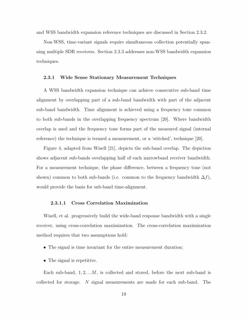
Figure 4, adapted from Wisell [21], depicts the sub-band overlap. The depiction
shows adjacent sub-bands overlapping half of each narrowband receiver bandwidth.
For a measurement technique, the phase difference, between a frequency tone (not
shown) common to both sub-bands (i.e. common to the frequency bandwidth ∆f),
would provide the basis for sub-band time-alignment.
2.3.1.1 Cross Correlation Maximization
Wisell, et al. progressively build the wide-band response bandwidth with a single
receiver, using cross-correlation maximization. The cross-correlation maximization
method requires that two assumptions hold:
• The signal is time invariant for the entire measurement duration;
• The signal is repetitive.
Each sub-band, 1, 2, ...M , is collected and stored, before the next sub-band is
collected for storage. N signal measurements are made for each sub-band. The
19
Figure 4. Bandwidth expansion using overlapping frequency bandwidths. Narrow-band receiver bandwidths (sub-bands) indicated by Mi, Mi+1, Mi+2 and Mi+3 withcenter frequencies f1, f2, f3 and f4, are overlapped using an internal reference. Sub-band spacing is denoted by ∆f and is represented as half the usable bandwidth [21].
signal measurements provide samples for an averaging process using least squares
estimation [21]. The averaging process is inconsequential to this research effort, but
is noted here to facilitate explanation of the equation variables. Each received sub-
band signal is down-converted and sampled.
A coarse time-domain cross-correlation is applied to effect time-alignment (sample-
based) of each sub-band. The time domain cross-correlation is,
∣∣∣∣∣n0,i+L−1∑n=n0,i
m0(n)m∗i (n− n0,i)
∣∣∣∣∣, (1)
where the discrete time domain signals, m0[n],m1[n], ...mM−1[n], each contain L sam-
ples, m0 is the initial collection, n(0,i) is the delay, based on the N time-aligned signal
measurements with regard to n0, and i = 1, 2, ...M − 1 [21].
The signal is then reconstructed in the frequency domain using the overlapping
parts of each sub-band. Each sub-band must first undergo a Discrete Fourier Trans-
form (DFT). For the upcoming discussion, M+i is the frequency domain representation
of the upper-half of the sub-band Mi and M−i+1 is the lower-half of the sub-band Mi+1.
20
The sub-bands, along with their center frequencies are identified in Figure 4 [21].
M+i and M−
i+1 are cross-correlated in the frequency domain. The spectral cross-
correlation is,
P−1∑k=0
M+i (k)[M−
i+1(k)e(−j2πkn(0,i+1))]∗, (2)
where P is the number of overlapping frequency bins, k is the frequency bin index and
n(0,i+1) is the delay, based on the N time-aligned signal measurements with regard
to n0, and i = 1, 2, ...M − 1 [21].
The maximum of (2) provides for the spectral alignment of M+i+1(k) (i.e. the upper-
half of the sub-band Mi+1(k)). M+i+1(k) is then concatenated with Mi(k) (i.e. M−
i+1(k)
is removed). The process is repeated for overlap M+2 (k) and M−
3 (k), through to
M+P−1(k) and M−
P (k) reconstructing the frequency spectrum of the time-aligned sub-
bands [21]. Smea(k) describes the frequency spectrum,
Smea(k) = [M1(k)M+2 (k)e(j2πkn0,2), ... ,M+
P (k)e(j2πkn0,P )], (3)
While the amount of overlap indicated here (∆f) is half a sub-band bandwidth,
the amount of overlap is not set. However, the overlap must include frequency tones
coincident to both sub-bands [21]. Once all adjacent sub-bands are aligned (3) un-
dergoes an Inverse Discrete Fourier Transform (IDFT) to restore the time domain
signal.
The cross-correlation maximization technique uses a single receiver to make con-
secutive sub-band collections. This would be unsuitable for this research effort as
21

the uniform white noise signal is time-varying. The need to collect signal sub-bands
over a period of time would not allow for accurate transmit signal reconstruction. To
overcome this issue, this research effort will use multiple SDRs. The SDR collection
times will be synchronized. Each SDR receives a different sub-band, with the sum of
sub-bands spanning the transmitted signal bandwidth.
A recent research effort successfully adapted the cross-correlation maximization
technique using two simultaneous SDR receiver collections [8]. Section 2.3.3 provides
further details regarding [8], including the need for simultaneous collection as the time-
invariant and repetitive signal assumptions did not hold.
2.3.1.2 Phase De-trending
The process of phase alignment is critical to bandwidth expansion signal recon-
struction. Remley, et al. apply a phase alignment technique known as ‘phase de-
trending’ to multisine signal frequency tones [22]. Phase detrending is a two-step
process that restores a reference time (tref ) by identifying the phase difference be-
tween two adjacent frequency tones at a specified measurement time (tm). The first
step provides a coarse time-shift estimate (tref−tm). The coarse time-shift estimate is,
(tref − tm)est =[θi+1(tm)− θi+1,exp]− [θi(tm)− θi,exp]
2π(fi − fi+1), (4)
where θi(tm) is the measured phase of the ith frequency tone, θi,exp is the expected
phase of the ith frequency tone and subscripts i and i + 1 again refer to adjacent
sub-bands [22]. The numerator identifies a phase difference between two frequency
tones. The phase difference falls between 0 and 2π.
Remley acknowledges the measured phase seldom reflects the expected phase due
to “signal generation, measurement and distortion errors” [22]. Therefore, the second
22

step refines the coarse estimate using an error minimization function to ‘detrend’ the
phase. The global error minimization function is,
E(t) =N∑i=1
|θi(t)− θi,exp|2, (5)
where N is the number of frequency tones [22]. The global minimum of (5) provides
the best estimate of tref . Here the linear phase shift in the frequency domain is con-
sidered as a delay in the time domain. In this manner, the delay can time-align or
restore tm to tref [22]. Once tref is restored, θi(tref ) for each frequency tone fi is,
θi(tref ) = θi(tm) + 2πfi(tref − tm), (6)
Remley, et al. state that phase alignment can be extended to other frequency
components [22], but it is not supported by provided examples, nor inferred that this
applies to all sub-band frequency components.
Remley’s (4) [22] coarse estimate relies on precise frequency fi and fi+1 for the
time-shift. Wisell’s (2) [21], Mi and Mi+1 sub-bands centered on frequency fi and fi+1
respectively, also rely on precise fi and fi+1 to locate the cross-correlation maximum
for the time-shift.
In summary, Remley’s phase detrending technique uses a consecutive collection
process and requires the signal to be repetitive. This is inconsistent with the re-
quirements for the uniform white noise signal that is intended for this research effort.
Importantly, Remley, et al. identify a critical issue that will affect our research ef-
fort. The issue is that an imprecise frequency correction will increase error, reducing
23

phase estimate accuracy. This is significant. Bandwidth expansion does not tolerate
frequency drift which is particularly acute with SDRs [9]. Frequency sensitivity to
local oscillator drift will need to be addressed in both single, dual and multiple SDR
cases.
2.3.2 Wide Sense Stationary Reference Techniques
A WSS bandwidth expansion technique achieving consecutive sub-band alignment
using a ‘pilot signal’ to time-align frequency tones is termed a reference technique [20].
Figure 5, adapted from [21], depicts the adjacent sub-band alignment. The pilot signal
and the individual frequency tones required for alignment are not shown.
2.3.2.1 Pilot Signals
Zenteno, et al. add a known a priori ‘pilot’ signal, for use as a time reference
to reconstruct a wide-band signal. The wide-band signal bandwidth extends beyond
the measured signal bandwidth of a single receiver. The pilot signal is added to the
signal of interest and must span each measured signal bandwidth [20]. The number
of receivers required to span the wide-band signal bandwidth is given by M .
The measured signal model is,
ri = xi + pi, (7)
where xi is the signal of interest and pi is the pilot signal and subscript i indexes
the ith measured sub-band used to reconstruct the wide-band signal [20]. Both xi
and pi are complex vectors of length N .
The frequency domain representation of the measured signal is,
24
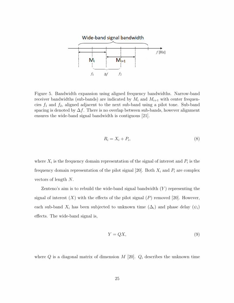
Figure 5. Bandwidth expansion using aligned frequency bandwidths. Narrow-bandreceiver bandwidths (sub-bands) are indicated by Mi and Mi+1 with center frequen-cies f1 and f2, aligned adjacent to the next sub-band using a pilot tone. Sub-bandspacing is denoted by ∆f . There is no overlap between sub-bands, however alignmentensures the wide-band signal bandwidth is contiguous [21].
Ri = Xi + Pi, (8)
where Xi is the frequency domain representation of the signal of interest and Pi is the
frequency domain representation of the pilot signal [20]. Both Xi and Pi are complex
vectors of length N .
Zenteno’s aim is to rebuild the wide-band signal bandwidth (Y ) representing the
signal of interest (X) with the effects of the pilot signal (P ) removed [20]. However,
each sub-band Xi has been subjected to unknown time (∆i) and phase delay (ψi)
effects. The wide-band signal is,
Y = QX, (9)
where Q is a diagonal matrix of dimension M [20]. Qi describes the unknown time
25
(∆i) and phase delay (ψi) effects on Xi [20]. Qi is,
Qi = Qi(∆i, ψi) = e(−j 2πkN
∆i+ψi)IN (10)
where kε[−N2, ...N
2− 1], N is the length of the measured signal complex vector and
I is an identity matrix of dimension N [20]. Estimating (∆i, ψi) for the M receivers
relies on a least squares approximation using the known pilot signal time delay and
phase delay as reference values. This allows the wide-band signal frequency domain
representation to be rebuilt. The approximation does not contribute to this research
effort and is not discussed here. A non-linear least squares technique is discussed in
Section 2.3.3. Once all adjacent sub-bands are aligned, the wide-band signal frequency
representation undergoes an IDFT to restore the time domain signal.
The pilot signal technique reduces receiver hardware requirements due to the
adjacent sub-band alignment [20]. This would be beneficial to this research effort.
The auto-correlation technique employed by this research exploits the use of adjacent
sub-band alignment vice overlapping sub-bands.
The pilot signal must span the wide-band signal bandwidth [20]. This places an
additional requirement on the signal generator. This research aims to reduce the
complexity of a developed NDE device. Exploiting the technique would involve a
trade-off between increasing transmitter complexity versus a reduction in the number
of SDR receivers.
The measured signal must also be repetitive [20]. This negates use of the intended
uniform white noise signal. For this reason the pilot signal technique is not used.
2.3.2.2 Wide Sense Stationary Signal Summary
The WSS bandwidth expansion techniques discussed in [20–22] are unsuitable for
time-variant signals. Aforementioned techniques require the signal to be repetitive.
26
The uniform white noise signal is not repetitive. A single receiver is also unlikely
to collect all sub-bands before the signal changes. The uniform white noise signal is
time-varying, rendering stored sub-bands unusable.
The WSS review has identified the need for precise frequency correction, to ensure
accurate phase estimates. The next section reviews non-WSS bandwidth expansion
techniques which are more closely aligned to our problem.
2.3.3 Non-Wide Sense Stationary Techniques
Time variance imposes two signal collection and processing requirements. First,
the entire signal must be collected simultaneously and second, if the entire signal is
collected as a series of sub-bands, sub-band frequency and phase must subsequently
be synchronized. The first requirement is achieved simply by determining the receiver
instantaneous bandwidth and calculating the number of SDRs required to span the
wide-band signal bandwidth. The second requirement is more problematic, with
consideration of time, frequency and phase synchronization needed.
Section 2.3.3 reviews non-WSS techniques used for frequency and phase synchro-
nization, including Phase Locked Loops, non-data aided feed-forward estimation and
phase correction using cross-correlation for simultaneously collected signals.
2.3.3.1 Phase Locked Loops
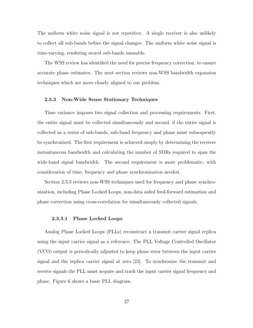
Analog Phase Locked Loops (PLLs) reconstruct a transmit carrier signal replica
using the input carrier signal as a reference. The PLL Voltage Controlled Oscillator
(VCO) output is periodically adjusted to keep phase error between the input carrier
signal and the replica carrier signal at zero [23]. To synchronize the transmit and
receive signals the PLL must acquire and track the input carrier signal frequency and
phase. Figure 6 shows a basic PLL diagram.
27

Figure 6. A Basic Phase Locked Loop Diagram [24].
In a steady-state, the phase detector determines phase difference (e(t)) between
the received input carrier signal (r(t)) and the VCO output replica carrier signal (x(t)).
The loop filter (f(t)), described by its Fourier response (F(ω)), removes higher fre-
quencies from (e(t)) before the linear filtered voltage is input to the VCO. The VCO
converts the linear filtered input voltage (y(t)) to the output replica carrier signal
(x(t)) accounting for any phase error. (x(t)) is input to the phase detector for the
next tracking loop evolution [24].
The digital PLL has component, implementation and performance differences but
serves the same purpose. Typically, a numerical controlled oscillator replaces the
VCO, the phase detector is replaced with a discriminator, and the digital equivalent
of an analog loop filter is applied.
Historically, communication systems used a feed-back mechanism for frequency
and phase synchronization. Early analog PLL complexity made the PLL “economi-
cally unfeasible” for most applications [19]. However, a recent research effort demon-
strated the use of a digital PLL applied to the bandwidth expansion problem [25].
The research effort reconstructed two overlapping frequency bandwidth receiver in-
puts. Neither receiver input spanned the full transmit signal bandwidth. The input
28

phases were synchronized, after pulse shaping, using a digital PLL. The digital PLL
incorporated a phase detector, loop filter and digital data synthesizer.
The GRC conference presentation [25] details for the research effort are not exten-
sive. However, experimental results with a Bit Error Rate (BER) better than 10−5 at
an Energy per Bit to Noise Power Spectral Density (Eb/N0)= 10 are indicated [25].
BER infers a communications signal, although this is not explicitly stated in [25]. This
research uses Symbol Error Rate (SER) versus Energy per Symbol to Noise Power
Spectral Density (Es/N0) metrics. Further symbol recovery measurement details are
found in Section 3.1.4.
PLLs provide accurate phase measurement but are susceptible to dynamic stress.
Dynamic stress presents as large variations in the input signal frequency. The Fre-
quency Locked Loop (FLL), while providing less accurate phase measurement, is
more tolerant to dynamic stress [23]. Kaplan describes a Global Positioning System
(GPS) digital carrier tracking loop implementation that uses a FLL assisted PLL or
‘pull-in’ technique [23]. FLL assisted PLL tolerates dynamic stress and retains phase
measurement accuracy. Figure 7 shows a basic FLL assisted PLL loop filter [23].
Figure 7. A first order frequency locked loop assisted second order phase locked loopdiagram [23].
FLL assisted PLL occurs in the digital loop filter. The initial phase inputs are
zeroed and a wide-band discriminator frequency error output is applied to establish
29
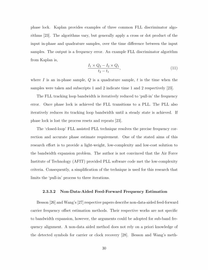
phase lock. Kaplan provides examples of three common FLL discriminator algo-
rithms [23]. The algorithms vary, but generally apply a cross or dot product of the
input in-phase and quadrature samples, over the time difference between the input
samples. The output is a frequency error. An example FLL discriminator algorithm
from Kaplan is,
I1 ×Q2 − I2 ×Q1
t2 − t1, (11)
where I is an in-phase sample, Q is a quadrature sample, t is the time when the
samples were taken and subscripts 1 and 2 indicate time 1 and 2 respectively [23].
The FLL tracking loop bandwidth is iteratively reduced to ‘pull-in’ the frequency
error. Once phase lock is achieved the FLL transitions to a PLL. The PLL also
iteratively reduces its tracking loop bandwidth until a steady state is achieved. If
phase lock is lost the process resets and repeats [23].
The ‘closed-loop’ FLL assisted PLL technique resolves the precise frequency cor-
rection and accurate phase estimate requirement. One of the stated aims of this
research effort is to provide a light-weight, low-complexity and low-cost solution to
the bandwidth expansion problem. The author is not convinced that the Air Force
Institute of Technology (AFIT) provided PLL software code met the low-complexity
criteria. Consequently, a simplification of the technique is used for this research that
limits the ‘pull-in’ process to three iterations.
2.3.3.2 Non-Data-Aided Feed-Forward Frequency Estimation
Besson [26] and Wang’s [27] respective papers describe non-data-aided feed-forward
carrier frequency offset estimation methods. Their respective works are not specific
to bandwidth expansion, however, the arguments could be adopted for sub-band fre-
quency alignment. A non-data aided method does not rely on a priori knowledge of
the detected symbols for carrier or clock recovery [28]. Besson and Wang’s meth-
30

ods, instead, exploit data embedded within the transmission signal, non-linear least
squares estimation and squaring loop principles to provide a frequency offset estimate.
A squaring loop establishes an index for carrier recovery. A received carrier with
signal level symmetric about zero does not provide useful information regarding the
transmitted carrier. Squaring the received signal generates power in a frequency
component at twice the carrier frequency. This frequency component can then be
filtered to provide an index for carrier recovery [29].
The model used by Besson [26] is,
y(t) = αx(t)ejω0t + e(t) t = 0, 1, 2, ..., (12)
where “α is a complex-valued amplitude, x(t) is a real-valued time-varying enve-
lope, ω0 is the frequency and e(t) is a disturbance” [26].
Besson finds a frequency estimate by manipulating a squared-loop application
of (12) to meet a non-linear least squares criterion. The least squares criterion is,
N−1∑t=0
|y(t)− αx(t)ejω0t|2, (13)
where N is the number of samples [26]. The squaring loop is repeated N times to
identify the ω0 that minimizes (13) [26].
The frequency offset estimation method derived in [26] applies the frequency es-
timate to a Binary Phase Shift Keying second order modulation. Wang applies a
variation of the estimation method to a Quadrature Phase Shift Keying (QPSK)
signal. QPSK modulation order requires fourth order values but the principles are
transferable [27].
Two key equations resulting from [27] are adopted for bandwidth expansion. The
first equation finds the global maximum, instead of the global minimum in [26], of a
31

least squares equation to provide a frequency estimate. The frequency offset estimate
derivation is provided in Appendix 5.1.4. The global maximum of the frequency es-
timate is,
fest =1
4
(1
N
N−1∑n=0
|ym(n)e−j2πf(n)|2), (14)
where m is the modulation order, n is the sample index, N is the number of sam-
ples, y is the received signal and f is the expected carrier frequency [27]. The second
equation applies the frequency estimate (14) to compensate for the frequency offset.
The frequency compensation equation is,
fcomp = y e−j2πfest(n), (15)
In practice, a QPSK received signal is raised to the fourth power, then undergoes
a DFT with a high oversampling rate (e.g. 223 S/s) [27]. The global maximum is
identified in the resultant frequency response. The position index at 14
the global
maximum position index is fest. Substituting fest of (14) into fcomp of (15) restores
the carrier frequency.
It was identified after the initial QPSK simulation, described in Section 3.1, that
the frequency offset estimation technique was not appropriate for the uniform white
noise signal. The technique exploits signal cyclo-stationary (CS) statistics. CS statis-
tics are readily found in M-ary shift keying signals [26,27] but are absent in noise.
32

2.3.3.3 Phase Correction of Simultaneous Collections
Accurate phase recovery requires a precise frequency overlap between adjacent
sub-bands. An ideal frequency overlap minimizes phase error attributable to fre-
quency mismatch. The phase correction technique described here was identified in a
recent AFIT research effort [8].
The frequency estimator (14) described in Section 2.3.3.2 can be used to provide
the position index for a QPSK frequency estimate. Alternately, as proposed in [8]
cross-correlating the frequency spectra of adjacent overlapping sub-bands will provide
a coarse position index. The position index identifies the frequency offset. Review of
the spectral cross-correlation technique shows similarities to the approach described
in Section 2.3.1.1, however (2) requires over-sampling to effect a least squares solution.
The spectral cross-correlation technique, used in [8], does not seek a non-linear least
squares solution.
The cross-correlation equation presented in [30] with time domain variables can
be substituted for frequency domain variables. This is due to the Fourier Time /
Frequency duality principle. The frequency domain cross-correlation is,
CXY [l] =∞∑−∞
X[k] Y ∗[k + l] −∞ < l < ∞, (16)
where X[k] are DFT coefficients of the first received sub-band, Y ∗[k+l] is the complex
conjugate of the DFT coefficients of the second received sub-band with frequency shift
[l] and ∗ is the complex conjugate [30]. CXY at lag [l] presents as a frequency shift.
The lag is applied to frequency align the sub-bands.
For phase correction, adjacent frequency domain spectra are overlapped using the
frequency cross-correlation technique described. The sub-band overlapping portions
are band-pass filtered before an IDFT restores the overlapping portions to the time
33

domain. The overlapping portions are then cross-correlated. The time domain cross-
correlation is,
Cxy[m] =∞∑−∞
x[n] y∗[n+m], −∞ < m < ∞, (17)
where x[n] is the first restored overlapping sub-band, y∗[n + m] is the complex con-
jugate of the second restored overlapping sub-band at delay [m] and ∗ is the complex
conjugate [30]. Cxy at lag [m] presents as a delay. The delay is applied to time-align
the sub-bands, not just the overlapping portions.
The research effort culminated in the reconstruction of a 2 MHz QPSK transmit
signal using two SDRs [8]. Each SDR was band-limited, able to recover a 1 MHz sub-
band. The SDR selected center frequencies provided a sub-band overlap of 20 kHz
resulting in a recombined signal spanning 1.98 MHz. The processed signal exhibited
accurate QPSK symbol recovery. The research did not extend the process to multiple
sub-bands, nor did it investigate the uniform white noise signals explored in this
research.
2.3.3.4 Non-Wide Sense Stationary Signal Summary
The non-WSS bandwidth expansion techniques use simultaneous signal collection
approaches. Further, the PLL and the simultaneous phase correction techniques
do not require a repetitive signal. However, each technique only provides a partial
solution to the current problem. The PLL technique requires complex code, the
frequency estimate technique is limited to M-ary signals and the phase correction
technique has not been proven across multiple sub-bands.
Consequently, this research effort attempted to develop the phase correction tech-
nique, in [8], to multiple sub-bands. As stated, the approach was abandoned in
34
favor of an auto-correlation technique. While it would be customary to include auto-
correlation background discussion here, the reader is directed to Section 3.2.1 and
Section 3.2.2 for further detail on the auto-correlation technique used in this research
effort.
2.4 Device Classification
Device characterization afforded by RF-DNA has its origins in authorized device
identification and rogue detection [31–33]. More recently, research efforts have shown
RF-DNA is suitable for fault condition characterization during device assembly, accep-
tance testing and in-service scenarios [2–7]. Generally, RF-DNA processing requires
signal collection, statistical fingerprint generation, device training and classification.
2.4.1 Signal Selection
As discussed, concurrent frequency spectrum use requires a non-intrusive inter-
rogation signal. A uniform white noise signal meets this requirement due its low
average power. Average power Pa, being a key determinant in signal detection [34],
is calculated as,
Pa = Ptτ
T, (18)
where Pt is peak power, τ is signal duration and T is the pulse repetition interval [35].
As can be seen, for fixed τ and T values Pa is determined solely by Pt [35]. Low Proba-
bility of Intercept (LPI) systems using a low-continuous Pt spread over the duty cycle
can achieve detection performance equivalent to conventional systems that use high
Pt and short τ . LPI systems mitigate low-continuous Pt by increasing τ until a unity
duty cycle is achieved [34]. The duty cycle is,
35

dc =τ
T. (19)
Consequently uniform white noise signal low peak-to-average power ratio and wide
bandwidth results in a signal that is difficult to detect and classify without a priori
knowledge. Further, a uniform white noise signal provides a uniformly distributed
power throughout the sampled spectrum (i.e. a ‘flat’ power spectral density) which
assists with DUT resonant response optimization [2]. These characteristics make the
uniform white noise signal a valid NDE stimulation signal candidate.
A uniform white noise signal is derived using repeated random variable sampling
from a uniform Probability Mass Function (PMF) defined as,
pu(r) = U(r; r1, r2) =
1
r2−r1 , r1 ≤ r ≤ r2
0, otherwise,
(20)
and is characterized by its mean (r) and variance (σ2r) [12]. The mean (r) for a uni-
form noise PMF is,
r =1
2(r2 − r1), (21)
and the variance (σ2r) for the uniform PMF is,
σ2r =
(r2 − r1)2
12. (22)
The development of the simulation and hardware test uniform white noise signal is
36

discussed further in Section 3.1.2.2.
2.4.2 Signal Collection
Signal collection requires a single SDR receiver or multiple SDR receivers depen-
dent on bandwidth recovery requirements. Bandwidth being the primary consider-
ation for improving signal reconstruction as identified in [6]. Lukac’s findings are
consistent with Hartley’s Law, where the information (I) gained is,
I ∝ β × τ, (23)
where β is the signal bandwidth and τ is the signal duration [19]. Assuming τ is
fixed, the information gained depends solely on the available bandwidth. Further
information on SDRs was provided in Section 2.2.
2.4.3 Fingerprint Generation
Fingerprint generation is reliant on features sourced from the collected signal [2–
4, 6, 7, 32]. Features are many and varied. Reviewed articles use instantaneous am-
plitude (a(t)), instantaneous frequency (f(t)) and instantaneous phase (φ(t)) [2–4,6,
7,32], Power Spectral Density [5], discrete Gabor transforms [5,33], complex wavelet
transforms [31] and slope-based Frequency Shift Keying (FSK) features [36].
Statistical variance (σ2), skewness (γ) and kurtosis (κ) are calculated for signal
feature sub-regions of interest. This reduces feature dimensionality, data storage and
processing duration [31]. Standard statistical equations for variance, skewness and
kurtosis of sequence x are given by,
σ2x =
1
Nx
Nx∑k=1
[x(k)− x]2, (24)
37

γx =1
σ3Nx
Nx∑k=1
[x(k)− x]3, (25)
κx =1
σ4Nx
Nx∑k=1
[x(k)− x]4, (26)
where x denotes the sequence mean value. The resultant statistics (24), (25) and (26)
are concatenated to form sub-region DNA markers,
FRi =[σ2xiγxi κxi
], (27)
where FRi is the regional feature vector and subscript i indicates the ith sub-region
[32]. These markers are concatenated to form RF-DNA characteristic fingerprints,
FC =[FR1 : FR2 : ... FR(NR+1)
], (28)
where : denotes vector concatenation, FC is the composite fingerprint vector and NR
is the number of sub-regions [32].
2.4.4 Device Training and Classification
RF-DNA composite fingerprint vectors are arbitrarily separated into two subsets;
a device training subset and a test (classification) subset. Multiple Discriminant
Analysis (MDA), a variation on the Fisher Linear Discriminant (FLD) analysis ap-
proach, is commonly applied in RF-DNA device training [2–4, 6, 31, 32, 36, 37]. The
purpose of discriminatory analysis being to separate samples into classes based on a
38
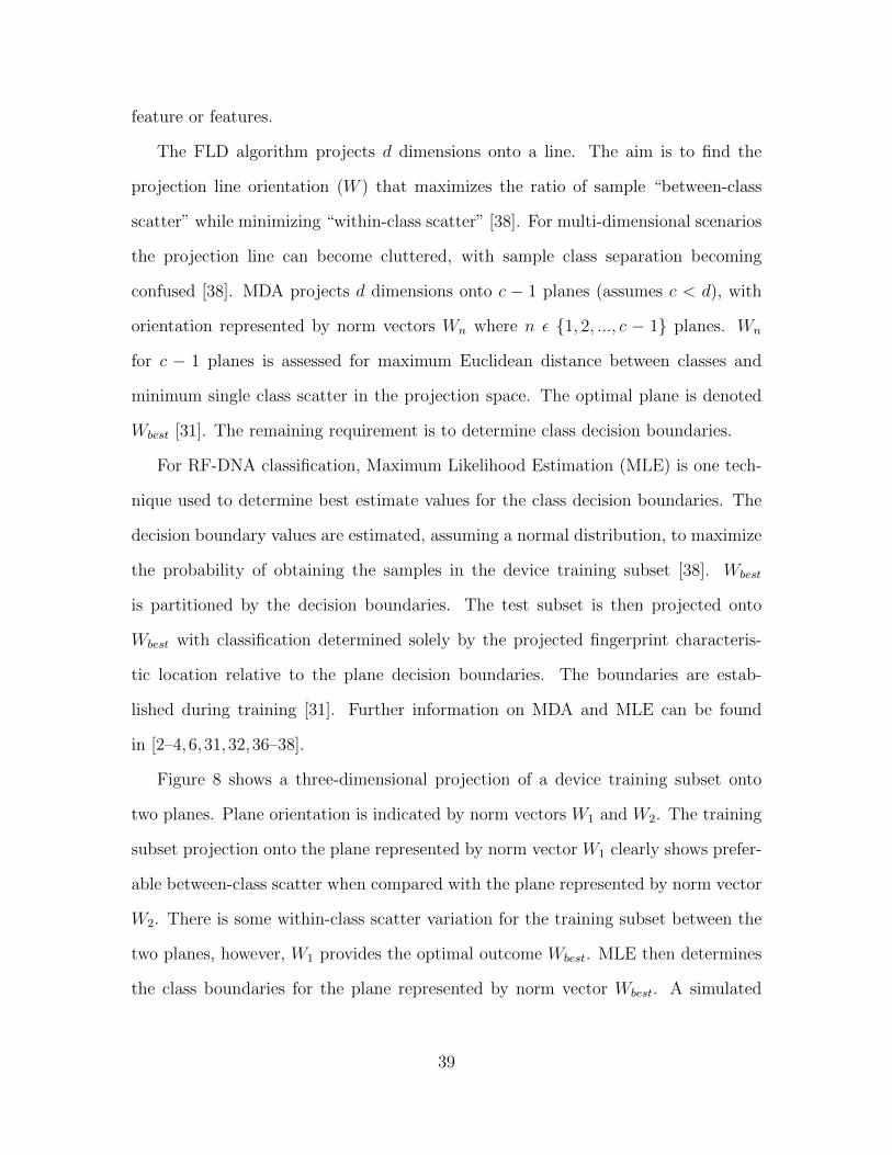
feature or features.
The FLD algorithm projects d dimensions onto a line. The aim is to find the
projection line orientation (W ) that maximizes the ratio of sample “between-class
scatter” while minimizing “within-class scatter” [38]. For multi-dimensional scenarios
the projection line can become cluttered, with sample class separation becoming
confused [38]. MDA projects d dimensions onto c − 1 planes (assumes c < d), with
orientation represented by norm vectors Wn where n ε 1, 2, ..., c − 1 planes. Wn
for c − 1 planes is assessed for maximum Euclidean distance between classes and
minimum single class scatter in the projection space. The optimal plane is denoted
Wbest [31]. The remaining requirement is to determine class decision boundaries.
For RF-DNA classification, Maximum Likelihood Estimation (MLE) is one tech-
nique used to determine best estimate values for the class decision boundaries. The
decision boundary values are estimated, assuming a normal distribution, to maximize
the probability of obtaining the samples in the device training subset [38]. Wbest
is partitioned by the decision boundaries. The test subset is then projected onto
Wbest with classification determined solely by the projected fingerprint characteris-
tic location relative to the plane decision boundaries. The boundaries are estab-
lished during training [31]. Further information on MDA and MLE can be found
in [2–4,6, 31,32,36–38].
Figure 8 shows a three-dimensional projection of a device training subset onto
two planes. Plane orientation is indicated by norm vectors W1 and W2. The training
subset projection onto the plane represented by norm vector W1 clearly shows prefer-
able between-class scatter when compared with the plane represented by norm vector
W2. There is some within-class scatter variation for the training subset between the
two planes, however, W1 provides the optimal outcome Wbest. MLE then determines
the class boundaries for the plane represented by norm vector Wbest. A simulated
39

classification test set projection is shown in Figure 9.
Figure 8. Multiple Discriminant Analysis three-dimensional sub-space projection ontotwo planes [39]. The two planes are identified by their norm vectors W1 and W2
which describe plane orientation. MDA aims to identify the plane orientation thatmaximizes between-class scatter (spreading) while minimizing within-class scatter(clustering) separation. The plane represented by norm vector W1 shows maximumbetween-class scatter and is selected in preference to the plane represented by normvector W2.
40
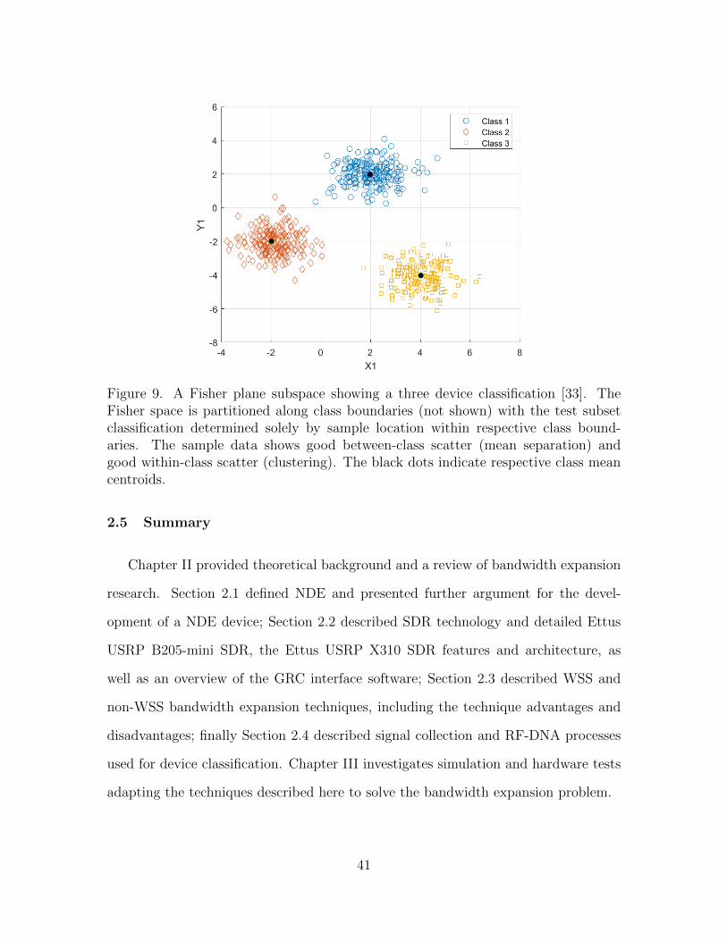
Figure 9. A Fisher plane subspace showing a three device classification [33]. TheFisher space is partitioned along class boundaries (not shown) with the test subsetclassification determined solely by sample location within respective class bound-aries. The sample data shows good between-class scatter (mean separation) andgood within-class scatter (clustering). The black dots indicate respective class meancentroids.
2.5 Summary
Chapter II provided theoretical background and a review of bandwidth expansion
research. Section 2.1 defined NDE and presented further argument for the devel-
opment of a NDE device; Section 2.2 described SDR technology and detailed Ettus
USRP B205-mini SDR, the Ettus USRP X310 SDR features and architecture, as
well as an overview of the GRC interface software; Section 2.3 described WSS and
non-WSS bandwidth expansion techniques, including the technique advantages and
disadvantages; finally Section 2.4 described signal collection and RF-DNA processes
used for device classification. Chapter III investigates simulation and hardware tests
adapting the techniques described here to solve the bandwidth expansion problem.
41

III. Methodology
The overarching goal of the research effort is to perform a wide-band signal re-
covery. The recovery involves collecting a wide-band uniform white noise signal that
exceeds the bandwidth of a single Software Defined Radio (SDR). This requires simul-
taneously collecting the signal using multiple SDRs. The reconstruction process must
account for frequency offset and phase errors to ensure accurate symbol recovery.
A general equation is proposed to determine the minimum number of SDRs (NSDR)
required to recover the full span of a transmitted signal bandwidth. The proposed
equation is,
NSDR =
⌈βtx
βrx − βol
⌉, 0 < βol < βrx, (29)
where β is the instantaneous bandwidth, subscript tx denotes the transmit signal,
subscript rx denotes each SDR receiver filtered signal and subscript ol denotes the
desired sub-band overlap.
To investigate the adequacy of the equation we need to confirm that the NSDR
required to span a transmission signal bandwidth (e.g. the Noise Radar Network
(NoNET) transmission bandwidth) is consistently determined using (29). Alterna-
tively, we may find that additional factors affecting NSDR are identified requiring
reconsideration of (29).
The following sections describe the research methodology. Section 3.1 describes
the bandwidth expansion models; Section 3.2 details the bandwidth expansion tech-
niques used to effect transmit signal reconstruction; Section 3.3 discusses single, dual
and multiple SDR simulation and hardware tests; Section 3.4 describes the scaling of
the bandwidth expansion technique; Finally, Section 3.5 details a Radio Frequency-
42

Distinct Native Attribute (RF-DNA) test case. A summary of the bandwidth expan-
sion simulations are provided in Appendix 5.1.4 Table 12 and the hardware tests are
provided in Appendix 5.1.4 Table 13.
3.1 Bandwidth Expansion Modelling
Simulation and hardware tests allow us to assess the effects of inputs on a process
or system. Simulation also permits us to alter and assess the effect of controllable
and uncontrollable factors on the process or system [39]. Multiple simulation or test
runs can identify dominant factors influencing the desired output. These factors
can then be accepted, controlled or mitigated [39]. Before this occurs system model
development is required.
A communications system signal process is provided as a simulation model. The
model steps are implemented in the Matrix Laboratory (Matlabr) 2018a software.
The model is discussed in Section 3.1.1. Quadrature Phase Shift Keying (QPSK)
signal and uniform white noise signal model generation are discussed in Section 3.1.2.
This discussion includes the use of a Linear Feed-back Shift Register (LFSR) for draw-
ing random samples. Section 3.1.3 describes the test used to validate the model for the
research effort. Finally, symbol recovery measurement is discussed in Section 3.1.4.
3.1.1 The Communications System Signal Process Model
The communications system signal process model was developed using Matlabr R2018a.
Initial development was coded using scripts until a fundamental process appreciation
was gained. To improve computational efficiency and increase function flexibility,
subsequent code was developed using the Matlabr R2018a communications system
toolbox. This sub-section presents the process model overview. Bandwidth expansion
techniques, simulation and hardware test set-up and signal parameters are addressed
43
in later sub-sections.
To simplify modelling, the signal process model was separated into transmit and
receive components. The transmit and receive process models are shown in Figures 10
and 11 respectively. The minor variations to the models arising from QPSK modula-
tion and demodulation are discussed in Section 3.1.2.1. The signal specific variations
to the models are not indicated in Figure 10 and Figure 11.
3.1.1.1 The Transmit Process Model
The transmit process begins with modulating uniformly distributed randomly
sampled bits to form a complex symbol. The random samples are generated using the
Matlabr R2018a communications system toolbox ‘comm.PNSequence’ system object.
This system object simulates a LFSR. The LFSR is described in Section 3.1.2.1. A
user-defined number of symbols are combined to form a complex signal channel, or
multiple complex signal channels.
The complex signal channels (e.g. ‘TxA’ and ’TxB’) are up-sampled and filtered us-
ing the Matlabr communications system toolbox ‘comm.RaisedCosineTransmitFilter’
system object. Up-sampling interpolates ‘zeros’ between existing samples. This in-
creases the effective sampling frequency. Interpolation filtering, referred to as pulse
shaping, is provided by a Raised Root Cosine (RRC) filter. The RRC filter provides
half of a transmit-receive filter combination forming a raised cosine filter. The RRC
filter minimizes Inter-Symbol Interference (ISI) [11].
The up-sampled and filtered signal channels are then frequency shifted. Filter-
ing and signal channel frequency shifting are critical to successful bandwidth expan-
sion and are discussed further in Section 3.2. The frequency shifted channels, when
summed, form a contiguous transmit signal bandwidth. Each transmit signal chan-
nel provides an auto-correlation template to recover part of the receive bandwidth
44
(sub-band). Transmit signal leading and trailing edge zero-padding is applied. This
separates the signal pulses as the GNU Radio Companion (GRC) repeats, or contin-
uously loops, the transmit signal when the process flow-graph is activated.
3.1.1.2 The Receive Process Model
Sub-band recovery is required when a single SDR receiver bandwidth does not span
the complete transmit signal bandwidth. SDR receivers (e.g. RxA’ and ‘RxB’) are
selected or ‘tuned’ to different center frequencies so sub-bands, cumulatively spanning
the transmit bandwidth, can be recovered. This ensures that transmit bandwidth
coverage is contiguous, similar to the coverage depicted in Figure 4 for a bandwidth
overlap case or Figure 5 for an adjacent alignment case.
Additive White Gaussian Noise (AWGN) is assumed to be imparted to the trans-
mit signal during propagation. The B205 SDRs receive the AWGN-affected transmit
signal after a propagation delay. The propagation delay is proportional to the propa-
gation distance between the transmitter and a receiver. The propagation delay values
therefore differ for each SDR receiver, but are assumed to be fixed for a SDR as time-
varying propagation delay is not expected due to the static positions of the X310 and
B205 SDRs [9].
A pre-determined sub-band time period, containing a single response pulse, is
isolated for signal processing. The isolated pulse undergoes sample rate conversion
using an anti-alias filter and down-sampling. Anti-alias filtering is provided by the
Matlabr communications system toolbox ‘comm.RaisedCosineReceiveFilter’ system
object receive RRC filter. This filter forms the second half of the transmit-receive
raised cosine filter combination identified in Section 3.1.1.1. Down-sampling uses
a decimation process whereby samples are removed at intervals determined by the
samples-per-symbol value.
45

Figure 10. Communications system transmit signal process model [9].
46

Sample rate conversion is followed by receive sub-band frequency synchronization.
The receive sub-band is auto-correlated with the equivalent portion of the transmitted
signal (33) [30]. This is in contrast with Everett’s method [8] which achieved frequency
synchronization between received sub-bands using spectral cross-correlation (16) [30].
Auto-correlation exploits a priori transmit signal knowledge. This is justified as
the transmit signal channel parameters can be retained as a ‘template’ for auto-
correlation. The technique is discussed in Section 3.2.
After frequency synchronization, phase synchronization is considered. To syn-
chronize phase between a received sub-band and the transmitted signal, overlapping
transmit and receive frequency bands are restored to the time domain. The lag
between the restored sub-bands is applied as a delay to the transmit signal. The
technique is discussed further in Section 3.2. Frequency and phase corrected signals
are frequency shifted to base-band and summed to recombine the sub-bands. Finally,
demodulation and symbol sequencing restore the initial transmitted symbols.
3.1.2 Signal Generation and Processing
To validate the communications system process model, the QPSK and uniformly
white noise signal models were generated as inputs.
3.1.2.1 QPSK Signal
The first validation simulation used an QPSK signal. QPSK is a digital com-
munication technique that maps bits onto a quadrature constellation as complex
symbols [19]. The QPSK signal is selected to validate simulation methodology be-
cause of the ease with which signal recovery can be quantified using Bit Error Rate
(BER) [19].
For the transmit process, the QPSK signals are generated digitally in Matlabr R2018a.
47

Figure 11. Communication system receive signal process model[9].
48

The QPSK parameters are detailed in Table 9. Figure 12 shows the base-band QPSK
signal frequency spectrum. Samples are randomly generated from a uniform distribu-
tion using the Matlabr R2018a communications system toolbox ‘comm.PNSequence’
system object. The output bits are mapped at base-band to a complex symbol constel-
lation using the Matlabr R2018a communications system toolbox ‘comm.PSKmodulator’
system object.
Table 9. Model validation QPSK signal parameters.
Description ValueSample rate 2 MS/s
Samples per symbol 4Number of samples 20000Number of symbols 5000Transmit bandwidth 1 MHz
Sample duration 500 nsSymbol duration 2 µsSignal duration 10 ms
The ‘comm.PNSequence’ system object outputs a LFSR generated pseudo-noise
binary sequence. The LFSR bit sequence is determined by the shift-register length,
tap positions and shift-register initial values known as ‘seed’ bits. The current state
of the shift-register is based on exclusive-or (XOR) gate feed-back bits tapped at
indicated polynomial sequence points. The XOR gate feed-back tapped bits are added
‘modulo-2’ and passed back to the input providing a new state at each clocked register
shift [24].
Maximal LFSR polynomial sequences can be selected to minimize sequence rep-
etition at user-defined shift-register lengths [24]. The LFSR taps are derived from
a 36-bit feedback polynomial sequence (x36 + x25 + 1). The pseudo-random samples
generated are maximal. The selected repetition period of 236− 1 could be considered
to provide a ‘true’ random noise output sequence for Non-Destructive Evaluation
49
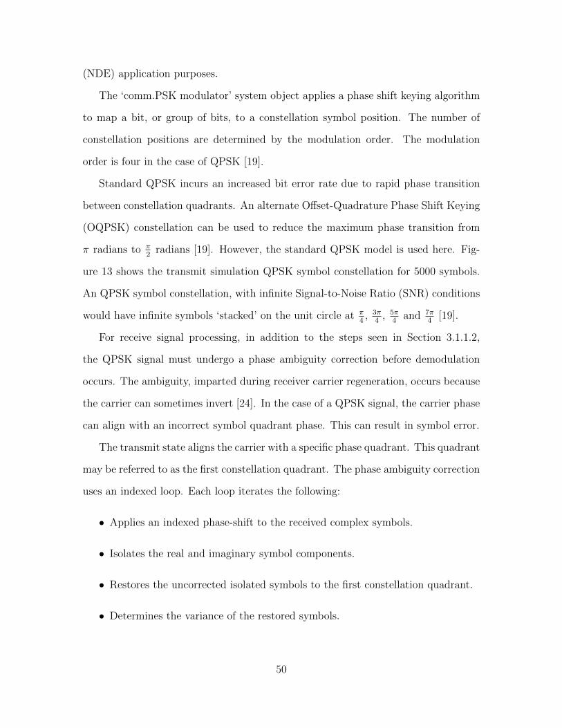
(NDE) application purposes.
The ‘comm.PSK modulator’ system object applies a phase shift keying algorithm
to map a bit, or group of bits, to a constellation symbol position. The number of
constellation positions are determined by the modulation order. The modulation
order is four in the case of QPSK [19].
Standard QPSK incurs an increased bit error rate due to rapid phase transition
between constellation quadrants. An alternate Offset-Quadrature Phase Shift Keying
(OQPSK) constellation can be used to reduce the maximum phase transition from
π radians to π2
radians [19]. However, the standard QPSK model is used here. Fig-
ure 13 shows the transmit simulation QPSK symbol constellation for 5000 symbols.
An QPSK symbol constellation, with infinite Signal-to-Noise Ratio (SNR) conditions
would have infinite symbols ‘stacked’ on the unit circle at π4, 3π
4, 5π
4and 7π
4[19].
For receive signal processing, in addition to the steps seen in Section 3.1.1.2,
the QPSK signal must undergo a phase ambiguity correction before demodulation
occurs. The ambiguity, imparted during receiver carrier regeneration, occurs because
the carrier can sometimes invert [24]. In the case of a QPSK signal, the carrier phase
can align with an incorrect symbol quadrant phase. This can result in symbol error.
The transmit state aligns the carrier with a specific phase quadrant. This quadrant
may be referred to as the first constellation quadrant. The phase ambiguity correction
uses an indexed loop. Each loop iterates the following:
• Applies an indexed phase-shift to the received complex symbols.
• Isolates the real and imaginary symbol components.
• Restores the uncorrected isolated symbols to the first constellation quadrant.
• Determines the variance of the restored symbols.
50

The variance from each iteration is stored in a vector. The global minimum of the
vector is applied as an index to phase-shift the received symbols. This provides the
phase corrected symbols for the first constellation quadrant. Subsequent quadrant
positions are found using indexed increments of π2, π and 3π
2radians to rebuild the
symbol constellation.
The Matlabr R2018a communications system toolbox ‘comm.PSKDemodulator’
system object is used for symbol demodulation, reversing the ‘comm.PSKmodulator’
system object process. Figure 14 shows a receive simulation QPSK symbol constella-
tion for 5000 symbols. The receive symbol constellation shows evidence of spreading
due to AWGN.
3.1.2.2 Uniform White Noise Signal
The second validation simulation substitutes the QPSK signal for a uniform white
noise signal. Uniform white noise is a non-intrusive interrogation signal due to its
low average power [34]. This is a key criteria for concurrent frequency spectrum use.
This is the reason that a uniform white noise signal is selected for this research effort.
The uniform white noise signal is generated digitally in Matlabr R2018a using the
parameters detailed in Table 10. Figure 15 shows the base-band uniform white noise
signal frequency spectrum.
Table 10. Model validation uniform white noise signal parameters.
Description ValueSample rate 2 MS/s
Samples per symbol 100Number of symbols 256Transmit bandwidth 2 MHz
Sample duration 500 nsSymbol duration 50 µsSignal duration 12.8 ms
51
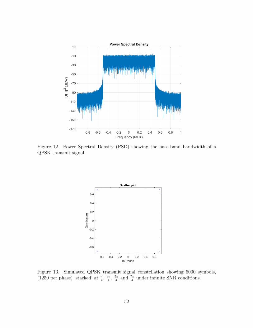
Figure 12. Power Spectral Density (PSD) showing the base-band bandwidth of aQPSK transmit signal.
Figure 13. Simulated QPSK transmit signal constellation showing 5000 symbols,(1250 per phase) ‘stacked’ at π
4, 3π
4, 5π
4and 7π
4under infinite SNR conditions.
52

Figure 14. Simulated QPSK received signal constellation, for a single pulse contain-ing 5000 symbols, after phase compensation. AWGN effects are evident but as themajority of symbols are restored to a quadrant, and assuming phase ambiguity isresolved, QPSK demodulation can commence.
Figure 15. PSD showing the base-band bandwidth uniform white noise transmitsignal.
53

The uniformly distributed white noise samples are generated using the Matlabr R2018a
communications system toolbox ‘comm.PNSequence’ system object. The output is
mapped to a P × Q symbol table, where P is the user-defined number of complex
symbols and Q is the user-defined symbol length. Complex symbols are randomly
drawn from the symbol table, without repetition, to form the uniform white noise sig-
nal. Drawing a complex symbol, without repetition, from the symbol table ensures
the random characteristic of the signal. The number of complex symbols R that de-
fine the signal is user-defined. Initial values of P , Q and R were set at 256 complex
symbol possibilities, a symbol length of 100, and 256 symbols per signal respectively.
3.1.2.3 Transmit Signal Spike Elimination
Everett identified a future work requirement to eliminate the transmit signal
‘spike’ attributed to clock bleed-through from the B205 SDR REF port to the TX/RX
port [8]. The spike is evident in frequency response figures presented in [8]. The trans-
mit spike is not evident in QPSK or uniform white noise hardware test cases for this
research effort. A spike was readily produced by introducing a DC bias into signal
generation code. The DC bias was introduced by the Matlabr ‘rand’ function during
symbol table generation. The ‘rand’ function produces values between 0 and 1. Both
real and imaginary values generated by the ‘rand’ function were offset by −0.5 to
remove DC bias. The resultant complex values have an expected mean of 0 + 0i.
Everett’s coding specific to the signal generation cases could not be located so
the clock bleed-through hypothesis was not eliminated as a causal factor. However,
if PSD plots present with the transmit spike, the possibility that the ‘rand’ func-
tion use has introduced a DC bias should be considered before reverting to the clock
bleed-through hypothesis. Alternatively, the Matlabr R2018a communications sys-
tem toolbox ‘comm.PNSequence’ system object and the Matlabr R2018a communi-
54
cations system toolbox ‘comm.PSKModulator’ system object.comm remove DC bias
automatically. Further, the SDR REF port should be terminated with an appropriate
load. The load impedance is typically detailed in the online user manual [40].
3.1.3 Signal Process Model Validation
For signal process model validation, a QPSK simulation and a uniform white noise
simulation were devised. The aim was to ensure communication system signal process
model inputs provided expected outputs when subjected to increasing AWGN. The
QPSK simulation and uniform white noise simulation both input a 500 kHz bandwidth
signal to the communications system signal process model.
A frequency shift of 260 kHz was applied to the QPSK signals, one positive
260 kHz shift and one negative 260 kHz shift to the respective channels using the
Matlabr R2018a communications system toolbox ‘comm.PhaseFrequencyOffset’ sys-
tem object. The same frequency shifts were applied to the uniform white noise sig-
nal simulation. The frequency shifts intentionally separate the two channel signal
frequency spectra to avoid symbol interference. This ensures unique bit sequence
demodulation. Typically, the aim of frequency shifting for bandwidth expansion is to
align adjacent sub-bands, or even provide an overlap.
The received symbols were sequenced by auto-correlating a stored replica of the
transmit symbols with the complex conjugate of the received symbols. This is simply
an adaption of the auto-correlation process to be discussed in Section 3.2. The se-
quenced symbols were then analyzed to provide Symbol Error Rate (SER). Section 4.2
provides the validation results.
55
3.1.4 Symbol Recovery Measurement
To provide process model output analysis, the probability of error for a given noise
degradation needs to be measured. The probability of error is then compared with
theoretical or simulated values. This identifies the penalty incurred by the bandwidth
expansion process in terms of the increased signal power required, or as will be seen,
the increased symbol power required.
For analog measurements, we are familiar with the probability of error versus SNR.
However, SNR is applicable for power signals. Digital signals are energy signals, with
probability of error typically presented as BER and SNR presented as Energy per
Bit to Noise Power Spectral Density (Eb/N0) [24]. For a complex input signal the
relationship between Eb/N0 and SNR is,
EbN0
=S
N
(W
R
), (30)
where Eb is the bit energy, N0 is the noise power spectral density, SN
is the SNR, W
is the bandwidth and R is the bit rate [24].
Information bits form the basis of digital messages. Eb/N0 allows the comparison
of one communication system with another at the information bit level [24]. Hence,
for a digital communication system Eb/N0 is a reasonable figure of merit.
This research effort is concerned with detection of the transmitted signal. As the
signal is digital, bit error could be selected as an analysis metric. However, dependent
on the number of information bits to each symbol, a bit error rate could be misleading.
As a simplified example, if a number of bits are in error in one symbol, the symbol
is in error. Alternately, if the same number of bits are in error, but those bits are
spread across multiple symbols, then each of those symbols are in error. This leads
to a difference in detection accuracy. Consequently, the probability of symbol error
56

is proposed as the preferred metric.
The probability of symbol error plots measure the SER versus Energy per Symbol
to Noise Power Spectral Density (Es/N0). The relationship between Es and Eb is,
Es = Eb(log2M), (31)
where Es is the symbol energy and M is the symbol set size [24]. Presenting Es/N0
in decibels, the relationship between Es/N0 and Eb/N0 is as follows,
Es/N0(dB) = Eb/N0(dB) + 10log10(k), (32)
where k is the number of information bits per symbol. The symbol set size can be
determined using k; i.e. M = 2k [24]. Therefore, Es/N0 adapts the SNR figure of
merit to provide a metric for our system analysis [24].
3.2 Bandwidth Expansion Techniques
The bandwidth expansion techniques used for this research effort rely on auto-
correlation. Auto-correlation is the correlation of a signal with itself, or more precisely
a delayed version of itself [30]. As we have a priori knowledge of the transmit signal,
auto-correlation can be used to recover the delayed version of the transmitted signal.
The auto-correlation function Rxx is,
Rxx[m] =∞∑−∞
x[n] x∗[n+m], −∞ < m < ∞, (33)
where x[n] is a stored replica of the transmit signal, x∗[n + m] is the complex con-
jugate of the transmit signal at a delay, or lag index [m], and ∗ denotes the complex
conjugate [30].
57

The auto-correlation lag index [m] can be exploited using the Fourier time-shift
property (34). The Fourier time-shift property is,
x[n−m] ⇐⇒ X[k]e−j2πk[n−m]
N , (34)
where the complex operator j =√−1 and k is the frequency index having pe-
riod N [30]. The lag index m is substituted in (34) to time-align the receive signal
sub-band with the equivalent portion of the transmit signal.
This is a common use for the Fourier time-shift property, and is used in this
research effort to time-align receive sub-bands with the equivalent portion of the
transmitted signal. This essentially identifies the receive signal sub-band start times.
The start time and a priori knowledge of the transmit signal length allows the receive
signal stop time to be determined. A more novel use was the application of auto-
correlation to a frequency ‘pull-in’ technique that aligns the transmit signal and the
receive signal sub-band frequency.
3.2.1 Auto-correlation - Frequency ‘Pull-In’
In Section 2.3.3.2 it was identified that the uniform white noise signal could not
exploit the non-data aided feed-forward carrier frequency offset estimation technique.
Therefore an auto-correlation technique using the transmit channel templates was
proposed. There is a duality to the time-shift property. This is the frequency-shift
property, which can be applied in the time domain to effect a frequency shift [30].
The Fourier frequency-shift property is,
x[n]ej2π[k−l]n
N ⇐⇒ X[k − l], (35)
58

where the complex operator j =√−1 and l is the shifted frequency index having
period N [30]. The auto-correlation principles can be transferred to the frequency-
shift property. The lag index here references the shifted frequency index [l]. The lag
index is substituted in (35) with opposite sign to frequency shift the receive signal
sub-band to align with the transmit signal.
The frequency-shift property provides the basis for the frequency ‘pull-in’ tech-
nique which adapts a Frequency Locked Loop (FLL) process found in [23]. The
‘pull-in’ technique uses three auto-correlation iterations. It was assumed that the fre-
quency offset would be a constant value between −20 kHz and 20 kHz for the short
duration (ms) signal. Section 4.3.1 show frequency change versus signal duration
results.
For the first ‘pull-in’ iteration each receiver frequency sub-band was auto-correlated
with the equivalent portion of the transmit signal. The transmit signal was swept
through the assumed frequency-shift range, centered on the transmit frequency in
100 Hz steps. The auto-correlation lag index identified the new center frequency for
the second iteration.
The second iteration used the same process as the first, except the auto-correlation
was effected between −100 Hz and 100 Hz of the new center frequency in 20 Hz steps.
The lag index identified the new center frequency for the third iteration.
The third iteration used the same process as the first and second iterations ex-
cept the auto-correlation was effected between −20 Hz and 20 Hz of the new center
frequency in 1 Hz steps. Due to the signal duration the FLL feed-back loop was not
closed [23]. Instead the third iteration lag index was applied to (35) with opposite
sign as a frequency shift and the FLL process ends.
59

3.2.2 Auto-correlation - Phase Correction
Phase correction also relies on auto-correlation. The phase correction technique
finds the angular difference between the inner product of two complex vectors. The
technique assumes that the angular difference is restricted to values between 0 and 2π
radians. An angular difference exceeding 2π would require the signal to be repetitive.
The uniform white noise signal is not repetitive. The technique also assumes that the
vectors are of equivalent length (M). The angle (θm) is,
θm = ∠M∑i=1
xi[n] x∗i [n+m], (36)
where ∠ denotes the angle operator, x[n] is a stored replica of the transmit signal,
and x∗[n+m] is the complex conjugate of the transmit signal at a delay, or lag index
[m]. ∗ denotes the complex conjugate and subscript i indexes the ith vector value [30].
The transmit signal replica x[n] and its delayed version x∗[n+m] are represented
by complex vectors. The angle (θm) returns a constant in radians. To phase-align the
complex vectors, θm is substituted into the following equation. The phase corrected
vector is given by,
x[n] = x[n+m] ejθm , (37)
where θm is substituted with opposite sign [30]. The phase correction is effected in
the phasor domain. The resultant shift also time-aligns the signal in the time domain.
3.2.3 Transmit Signal Preparation
The QPSK and uniform white noise transmit signal channels were designed in
Matlabr R2018a using a RRC pulse shaping filter. Table 11 details the RRC filter
60

parameters. The RRC filter design features a steep roll-off and reduced pass-band
ripple. This defines the characteristic square-like filter pass-band system response.
The adjacent channels can be aligned to provide a contiguous pass-band with band-
width overlap limited to that part of the response beyond the cutoff frequency. The
received sub-bands retain this characteristic simplifying signal reconstruction. Fig-
ure 16 shows the Matlabr FVtool depiction of the RRC filter frequency response. The
roll-off, using inputs from Table 9 is −3dBW/1000Hz. Figure 17 shows the resultant
frequency response of a pulse shaped QPSK signal transmit channel.
Table 11. RRC filter parameters for transmit signal preparation.
Description ValueFilter type Finite Impulse Response (FIR)
Response type Low-passSample rate 2 MS/sFilter span 400
Filter roll-off factor 0.01Samples-per-symbol (QPSK) 4Samples-per-symbol (noise) 2
Dynamic range 60 dBW
The channels are then frequency shifted to create the transmit signal. The fre-
quency shifts must be precise to ensure adjacent pass-bands are contiguous but do
not overlap. Section 3.3 identifies frequency shift values for single, dual and multiple
SDR simulation and hardware tests.
61

Figure 16. Matlabr FVtool filter depiction showing the steep filter roll-off used tominimize bandwidth overlap between adjacent receive signal sub-bands. Using theinputs from Table 11 the roll-off is −3 dBW/1000 Hz.
Figure 17. Filtered 1 MHz uniform white noise signal sub-band for transmit signalconstruction. The steep roll-off is a pre-requisite for successful bandwidth expansionusing the auto-correlation technique.
62

3.3 Bandwidth Expansion Application
Attempts were made to replicate the QPSK phase cross-correlation bandwidth
expansion technique in [8]. Phase cross-correlation [8], and the carrier frequency
offset estimation technique [26, 27] described in Section 2.3.3 produced error values
between 3% and 52%. Error values were obtained from trials, not controlled tests,
but the error range suggested issues with the replication approach. Regardless, the
earlier research efforts were abandoned due to the inconsistent error and the promising
indications offered by an auto-correlation technique. The auto-correlation technique
exploits a priori transmit signal knowledge and minimizes bandwidth overlap. The
QPSK and uniform white noise signal simulations and hardware tests are devised to
assess the auto-correlation bandwidth expansion techniques.
For the hardware tests, the transmit SDR is referenced to a 5 Vpp 10 MHz square
wave signal. This timing signal is sourced from an external Analog Waveform Gener-
ator (AWG) or the X310 on-board Global Positioning System Disciplined Oscillator
(GPSDO). The GPSDO is synchronized to the GPS constellation. A 1 Pulse Per
Second (PPS) clock signal is also sourced from the X310 on-board GPSDO. The on-
board GPSDO is selected for both timing and clock signals as the AWG does not
provide consistent results.
The GPSDO/AWG performance variation was not investigated. However, phase
noise is suggested as a possible cause. This is based on the quoted Agilent 33250A
AWG phase noise at 10 MHz of less than −65 dBc (30 kHz band) [41] versus the board
mounted OCXO GPSDO phase noise at 10 MHz of less than −145 dBc (10 kHz band)
adjusted to −105 dBc (30 kHz band) [17].
The B205 SDR receiver clock timestamp synchronization is provided by a 1 PPS
signal sourced from the X310 on-board GPSDO. The 1 PPS signal is passed via the
X310 PPS/TRIG OUT output port to the B205 REF port. The B205 can also accept
63

the 5 Vpp 10 MHz square wave timing signal. However, the B205 REF port supports
only one input, either the 10 MHz square wave or the 1 PPS signal. The 1 PPS signal
is selected for sample time synchronization. Frequency synchronization is addressed
using the auto-correlation technique.
Signal transfer is controlled by the GRC interface software. The txFile.bin file
is passed via the host-PC 1 Gigabit Ethernet (1G ETH) port to the X310 SDR for
digital-to-analog conversion before transmission at the RF front-end. The transmit
X310 SDR Tx/Rx port is connected to a receive B205 SDR via the B205 Rx2 port.
A 1 m Sub-Minature Version A (SMA) coaxial cable, SMA connectors and a Mini
Circuits 15542 30 dB 50 ohm load attenuator for receiver protection also form part
of the circuit. The input power into the B205 SDR was not quantified with the load
attenuator in position.
Receiver data is returned to Matlabr as an rxFile.bin file, The rxFile.bin file is
passed via a USB 3.0 cable, facilitated by the GRC interface software to the host-PC
for signal processing.
Sections 3.3.1, 3.3.2 and 3.3.3 describe the respective single, dual and multiple
SDR simulations. Sections 3.3.4, 3.3.5 and 3.3.6 describe the respective single, dual
and multiple SDR hardware tests.
3.3.1 Single Receiver Dual Channel Simulations
The single-receiver, dual-channel simulations aim to recover a 2 MHz transmit
bandwidth. The use of two channels allows the summation process to be tested. All
simulations and tests require summation to recombine received signal sub-bands. The
exception is the single-receiver, single-channel hardware test. The partitioning of the
transmit signal also provides the necessary templates to auto-correlate the equivalent
portion of the received signal.
64
The simulation is initially conducted with zero frequency offset and phase error.
As the frequency offset and phase error are not coded into the single receiver simula-
tion, frequency and phase alignment between the recovered channels and the transmit
signal is expected. Visually, auto-correlation plots are expected to identify zero lag,
requiring no subsequent correction.
For the QPSK and uniform white noise signal dual channel simulations, the sample
rate is set at 2 MS/s. Two simulated 1 MHz bandwidth transmit channels are gen-
erated using the transmit process model. The center frequency offsets of −0.5 MHz
and 0.5 MHz are applied. The transmit channels are summed to create a contiguous
2 MHz bandwidth signal.
The simulated 1 MHz bandwidth receive channels have center frequency offsets of
−0.5 MHz and 0.5 MHz applied respectively. The receive channels are generated to
collect the adjacent 1 MHz transmit signal portions. The collected signals are passed
through the receiver process model. The single-receiver, dual-channel simulation re-
sults are detailed in Section 4.2.1.
3.3.2 Dual Receiver Simulations
The dual SDR receiver simulations use a similar set-up to the single SDR receiver
simulations. Both the QPSK and uniform white noise signal simulations retain the
2 MS/s sample rate and the center frequencies at −0.5 MHz and 0.5 MHz respectively.
Random frequency offsets and phase error values are introduced to each signal to
simulate SDR local oscillator variation. The frequency offset (−20 to 20 kHz) and
phase error (−π to π radians) values are typical of preliminary B205 SDR performance
observations.
The auto-correlation ‘pull in’ technique described in Section 3.2.1 is applied to
correct the simulated frequency offsets. The auto-correlation phase correction tech-
65
nique described in Section 3.2.2 is applied to correct the simulated phase errors. The
dual receiver simulation results are detailed in Section 4.2.1.
3.3.3 Multiple Receiver Simulations
To test scalability, the multiple (i.e. four) SDR receiver simulations repeat the
process established for the dual SDR receiver simulations with minor changes. Again,
both the QPSK and uniform white noise signals are simulated. The transmit and
receive 1 MHz channel spacing is retained, with the sampling rate increased to 4 MS/s.
New transmit and receive channel center frequencies are established at -1.5 MHz,
−0.5 MHz, 0.5 MHz and 1.5 MHz. This provides a contiguous 4 MHz transmit
bandwidth. The transmit bandwidth is collected by four simulated SDRs, each with
a receive bandwidth of 1 MHz. The multiple receiver simulation results are detailed
in Section 4.2.2.
3.3.4 Single Receiver Hardware Tests
The single receiver hardware test methodology is discussed below. Section 3.3.4.1
considers a single channel methodology. This test is used to demonstrate the band-
width expansion problem. Section 3.3.4.2 considers an emulated dual channel method-
ology. This tests the transmit and receiver signal auto-correlation techniques and
bandwidth summation.
3.3.4.1 Single Receiver Single Channel Tests
A single-receiver, single-channel hardware test is devised. The aim of this test
is to show that a wide-band signal can not be faithfully reconstructed from a single
B205 SDR collection. The test assumes that the wide-band signal is time-variant
and therefore requires simultaneous collection of the transmitted signal bandwidth.
66
The test also assumes that the wide-band signal bandwidth exceeds the instantaneous
receiver bandwidth.
For the first part of the test a uniform white noise signal with a 50 MHz bandwidth
is generated. 50 MHz is selected as the bandwidth spans the majority of the B205 SDR
instantaneous bandwidth (50 MHz of 56 MHz). 50 MS/s also meets the X310 SDR
sample rate master clock decimation requirements. The X310 master clock is set
at 200 MS/s. 50 MS/s will provide an even integer decimation ratio of 4. The
sample time is synchronized across the transmit and receive SDRs. The transmit
and receive SDRs clock timestamp synchronization references the GPSDO 1 PPS
timing signal. A single B205 SDR receiver, identified as ‘RxA’, is prepared for the
hardware test. RxA variables are set in the GRC for a 50 MHz bandwidth with a
center frequency at 2.4 GHz. The Matlabr and GRC transmit and receive sampling
rate is set at 50 MS/s. The GRC interface software frequency shifts the transmit
signal from base-band to 2.4 GHz for transmission.
‘RxA’ captured the 50 MHz transmit bandwidth. Full symbol recovery for the
50 MHz bandwidth signal is expected, as this falls within the instantaneous bandwidth
of a B205 SDR. This will be confirmed by auto-correlating the transmitted symbols
with the received symbols. The results are provided in Section 4.3.1.
For the second part of the test a second signal is transmitted. The transmit signal
has a 100 MHz bandwidth. The 100 MHz bandwidth is selected because the signal
spans approximately twice the instantaneous bandwidth of the B205 SDR (100 MHz
versus 56 MHz). The X310 SDR sample rate master clock decimation requirements
are also met. 200 MS/s will provide an even integer decimation ratio of 2. The
signal is again transmitted at a 2.4 GHz center frequency and collected using ‘RxA’.
The Matlabr and GRC transmit sampling rates are set at 100-MS/s. Attempts to set
the ‘RxA’ sampling rate to 100 MS/s resulted in the GRC flow-graph process timing
67
out before a collection could be made. This is discussed further in the results. The
receive sampling rate was therefore restored to 50 MS/s.
Full symbol recovery for the 100 MHz bandwidth signal is not expected, as this
exceeds the B205 SDR instantaneous bandwidth. Symbol recovery will be confirmed
by auto-correlating the transmitted symbols with the received symbols. The single
SDR hardware test circuit is depicted in Figure 18. The GRC interface setup for
the single SDR hardware test is shown in Figure 19. The sampling rates indicated
are for the dual-channel tests. Single receiver hardware test results are detailed in
Section 4.3.1.
3.3.4.2 Single Receiver Dual Channel Tests
Two single-receiver, dual-channel hardware tests were devised. The tests use a
single receiver, with two emulated channels. The first test compared the bandwidth
expansion QPSK signal PSD with the simulation data. The second test compared
bandwidth expansion uniform white noise signal symbol recovery with a simulated
single-receiver, single-channel transmit signal recovery and the preceding QPSK signal
PSD.
The QPSK dual channel hardware test aims to recover a 2 MHz QPSK transmit
signal using a single SDR receiver. While the B205 SDR receiver bandwidth can
support a 2 MHz bandwidth on a single channel, two emulated channels, identified
as ‘RxA low channel’ and ‘RxA high channel’, are generated to test the bandwidth
expansion techniques. RxA low channel has a 1 MHz bandwidth with GRC center
frequency at 2.3995 GHz, while RxA high channel has a 1 MHz bandwidth with GRC
center frequency at 2.4005 GHz. The GRC transmitter sampling rate and receiver
sampling rate is set at 2 MS/s. The GRC interface software frequency shifts the
transmit signal from base-band to 2.4 GHz for transmission.
68

Receiver narrow-band sub-channel data is returned to Matlabr as rxFile(x).bin
files, where ‘x’ represent the low channel or high channel. The rxFile(x).bin files are
passed via a USB 3.0 cable facilitated by the GRC interface software to the host-PC
for signal processing.
The dual channel hardware test subjects the transmit signal and the SDR receive
signal to the transmit, environment, and receive variables that were previously con-
trolled during simulation. Frequency offset and phase error between the two receive
channel collections and the transmitted signal templates now need to be resolved
using the auto-correlation techniques.
The single SDR hardware test circuit is depicted in Figure 18. The GRC interface
setup for the single SDR hardware test is shown in Figure 19. Single receiver hardware
test results are detailed in Section 4.3.1.
Figure 18. Hardware circuit setup for single SDR receiver tests. Connection legend:TX/RX signal (Red); 1 PPS (Green); 1G ETH (Yellow); USB 3.0 (Blue).
3.3.5 Dual Receiver Hardware Tests
Two dual receiver hardware tests were initially devised. The first test aimed
to recover a 2 MHz QPSK transmit signal using two SDR receivers, each receiver
69

Figure 19. GNU radio companion interface setup for single SDR hardware tests.
recovering 1 MHz of the transmit signal. This test aimed to confirm the bandwidth
expansion technique was viable using hardware, accounting for additional receiver
frequency offset and phase errors arising from dual SDR receiver use.
The first dual receiver hardware test compared the bandwidth expansion QPSK
signal PSD with simulation data. The second test substituted the uniform white
noise signal for the QPSK signal. This test compared symbol recovery data with the
simulated single-receiver, single-channel uniform white noise signal symbol recovery
data and the QPSK signal PSD.
The sample time is synchronized across the transmit and receive SDRs. The
transmit and receive SDR clock timestamp synchronization again references a 1 PPS
timing signal. Two B205 SDR receivers, identified as ‘RxA’ and ‘RxB’, are prepared
for hardware tests. RxA had a 1 MHz bandwidth with the GRC center frequency at
70

2.3995 GHz, while RxB had a 1 MHz bandwidth with the GRC center frequency at
2.4005 GHz. The Matlabr and the GRC transmitter sampling rate is set at 2 MS/s
and the two receivers have sampling rates set at 1 MS/s. The GRC interface software
frequency shifts the transmit signal from base-band to 2.4 GHz for transmission. The
frequency shift ensures the signal is transmitted at frequencies supported by both the
X310 and B205 SDRs. ‘RxA’ captures the lower 1 MHz of the transmit bandwidth,
while ‘RxB’ captures the upper 1 MHz of the transmit bandwidth. Frequency offset
settings provide a bandwidth overlap. However, the overlap only occurs where the
transition region imposes on the adjacent sub-band. The frequency offset settings are
assumed to provide a contiguous 2 MHz bandwidth recovery.
Transmit signal propagation was similar to the single SDR case, except for minor
hardware changes. The hardware changes included a NARDA 4315 power splitter, a
USB3.0 multi-port adapter and additional cabling inserted into the circuit to support
the additional B205 SDR. The power splitter supported a bandwidth between 8 −
12 GHz. It is acknowledged that the transmit signal bandwidth was outside this
range. The impact of the incorrect frequency use (2.4 GHz) on the power splitter
signal output was not characterized. Additionally, the power loss attributable to the
splitter was not accounted for in Matlabr code to remove bias from SER plots. The
received signals were again passed via USB 3.0 to the host laptop Matlabr software
for signal processing.
The hardware test circuit is depicted in Figure 20. The GRC interface setup for
the dual SDR hardware test is shown in Figure 21. The 20 MHz and 100 MHz dual
SDR receiver cases are discussed in Section 3.4. The dual receiver hardware test
results are detailed in Section 4.3.2.
71
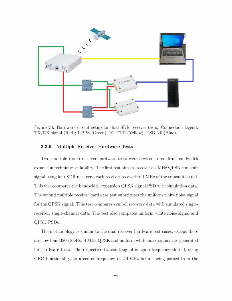
Figure 20. Hardware circuit setup for dual SDR receiver tests. Connection legend:TX/RX signal (Red); 1 PPS (Green); 1G ETH (Yellow); USB 3.0 (Blue).
3.3.6 Multiple Receiver Hardware Tests
Two multiple (four) receiver hardware tests were devised to confirm bandwidth
expansion technique scalability. The first test aims to recover a 4 MHz QPSK transmit
signal using four SDR receivers, each receiver recovering 1 MHz of the transmit signal.
This test compares the bandwidth expansion QPSK signal PSD with simulation data.
The second multiple receiver hardware test substitutes the uniform white noise signal
for the QPSK signal. This test compares symbol recovery data with simulated single-
receiver, single-channel data. The test also compares uniform white noise signal and
QPSK PSDs.
The methodology is similar to the dual receiver hardware test cases, except there
are now four B205 SDRs. 4 MHz QPSK and uniform white noise signals are generated
for hardware tests. The respective transmit signal is again frequency shifted, using
GRC functionality, to a center frequency of 2.4 GHz before being passed from the
72

Figure 21. GNU radio companion interface setup for dual SDR receiver hardwaretests.
host-PC to the X310 SDR for transmission. The B205 SDR receivers, ‘RxA’,‘RxB’,
‘RxC ’ and ‘RxD’ have center frequencies of 2.3985 GHz, 2.3995 GHz, 2.4005 GHz
and 2.4015 GHz respectively. Matlabr and GRC transmitter sampling rates are set
at 4 MS/s and GRC receiver sampling rates are set at 1 MS/s.
The hardware and Matlabr software changes simply scale existing B205 SDR sup-
port requirements. General connectivity, hardware application and synchronization
requirements were similar to dual receiver hardware test cases. The hardware test
circuit is depicted in Figure 22. The GRC interface setup for the four SDR hardware
test is shown in Figure 23. The 20 MHz and 100 MHz multiple SDR receiver cases
are discussed in Section 3.4. Test results are detailed in Section 4.3.3.
73

Figure 22. Hardware circuit setup for multiple SDR receiver test. Connection legend:TX/RX signal (Red); 1 PPS (Green); 1G ETH (Yellow); USB 3.0 (Blue).
74
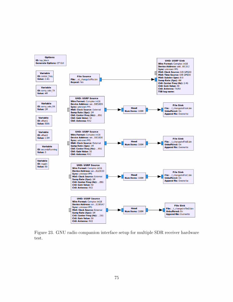
Figure 23. GNU radio companion interface setup for multiple SDR receiver hardwaretest.
75

3.4 Scaling the Bandwidth Expansion Technique
After the initial bandwidth expansion hardware tests the focus shifted to increas-
ing single SDR bandwidth use. This was followed by bandwidth expansion exceeding
a single SDR instantaneous bandwidth. A simple sampling rate adjustment and a
center frequency recalculation are the only variable changes required to extend the
recoverable bandwidth limits. The changes are applied to each sub-band.
Initially, a 50 MHz bandwidth hardware test was conducted using the dual SDR
hardware test set-up in Figure 20. The test repeatedly failed to recover the correct
symbol sequence. Each collection spanned a 25 MHz bandwidth. The GRC Graphic
User Interface (GUI) displayed an overflow (‘O’) condition which was interpreted as
the host-PC losing data packets. Reducing the bandwidth to 20 MHz resolved the
issue. For the 20 MHz test, each SDR collection spanned a 10 MHz bandwidth.
The reason for the unsuccessful 50 MHz test was investigated. Insufficient us-
able instantaneous bandwidth was identified as the cause. The usable instantaneous
bandwidth is governed by:
• SDR analog bandwidth.
• Field Programmable Gate Array (FPGA) processing bandwidth.
• Host-PC hardware bandwidth limitations [42].
Therefore, with the existing configuration, a 20 MHz bandwidth is reasonably ex-
pected to be the upper-bound of bandwidth expansion. The existing configura-
tion is comprised of an X310 SDR Universal Software Radio Peripheral (USRP)
UBX-160 daughter-board, FPGA processing bandwidth (Analog to Digital Converter
(ADC)/Digital to Analog Converter (DAC) (200/800 MS/s)) and a host-PC 1G ETH
hardware connection. The host-PC 1G ETH stream at 25 MS/s is the limiting factor
for this case [42].
76

The 20 MHz signal was the widest bandwidth successfully tested using the 1G
ETH connection. This was due to the aforementioned 1G ETH configuration and
the X310 SDR sampling rate decimation requirements. The X310 SDR sample rate
decimation is required to be an even integer value of the SDR master clock (e.g. When
the X310 SDR clock rate is set at 200 MS/s, a decimation rate of 10 will provide a
20 MHz bandwidth). The B205 SDR clock rate is set anywhere between 5 MS/s and
61.44 MS/s. The B205 SDR clock rate is determined automatically using a value
that ensures anti-aliasing and correct sample rate decimation is effected in the B205
SDR digital signal processor [40]. A multiple SDR recovery was also conducted for
the 20 MHz uniform white noise signal. Each collection spanned a 5 MHz bandwidth.
To expand the bandwidth beyond 20 MHz, a new host-PC with a 10 Gigabit
Ethernet (10G ETH) connection was sourced. Recall, that the 1G ETH was the
limiting factor with the preceding configuration. The substitution of the old host PC
with the new host-PC, and the inclusion of 10G ETH cabling and connections, were
the only changes to the hardware setup in Figures 20 and 22.
A 100 MHz bandwidth dual SDR recovery was tested. For the dual SDR recov-
ery, the sub-band collections each spanned the majority of a B205 SDR instantaneous
bandwidth (50 of 56 MHz). The X310 SDR USRP UBX-160 daughter-board is iden-
tified as the limiting factor for this hardware test. However, the daughter-board is
capable of supporting a 100 MHz transmit signal. Section 4.3.2 shows the dual SDR
results.
Following the dual SDR recovery, a multiple SDR recovery was conducted for the
100 MHz uniform white noise signal. Each collection spanned a 25 of 56 MHz of a
B205 SDR instantaneous bandwidth . The 100 MHz transmit signal bandwidth was
again selected due to X310 SDR USRP UBX-160 daughter-board filter roll-off atten-
uation and X310 sample rate decimation requirements (i.e. 200 MS/s decimation by
77
2 provides 100 MHz bandwidth). The 100 MHz bandwidth was the widest bandwidth
tested. Section 4.3.3 shows the multiple SDR results.
3.5 RFDNA Test Case
A three-class discrimination problem is proposed. The aim is to discriminate three
MiniCircuits 15542 30 dB 50 Ω load attenuators (S/Nos 31420 31647 31730) using the
uniform white noise interrogation signal. Single, dual and multiple SDR collections
are required. The set-up for a single SDR case is shown in Figure 18. The dual SDR
case is shown in Figure 20 and the multiple SDR case is shown in Figure 22.
The RF-DNA test case was not actioned, but the details are retained to facilitate
future work. The intended experiment for the single, dual and multiple SDR collection
required for one of the test attenuators (Device Under Test (DUT)) to be inserted
into the SDR transmit/receive loop. The attenuator is positioned after the X310
TX/RX port but before the power divider for each classication evolution. A 50 MHz
bandwidth, 1000 burst uniform white noise interrogation signal stimulates the DUT,
with collected data saved as a .mat Matlabr file.
The three .mat files are passed as input signal structures to Air Force Institute
of Technology (AFIT) Matlabr Burst.m and InSigStruct Creator.m code for signal
preparation, followed by fingerprint generation using AFIT Matlabr FingerPrint-
GenV14 code to generate a Matlabr finger-print feature .mat file. Finally, device
training and classication is provided by AFIT MDAML V14 code to provide 2-D
training and test Fisher projection plots and confusion matrices. Classification re-
sults and analysis were to be provided in Section 4.4.
78
3.6 Summary
Chapter III described the research effort methodology. Bandwidth expansion mod-
els, including the communications system signal process model, QPSK and uniform
white noise signal generation models and symbol recovery metrics were described.
Bandwidth expansion auto-correlation techniques and transmit signal preparation
details were provided and bandwidth expansion single, dual and multiple SDR sim-
ulations and hardware tests were outlined. Finally, an RF-DNA test case was sug-
gested as a real-world application for the bandwidth expansion process. Chapter IV
will provide results and analysis.
79

IV. Results and Analysis
The following sections provide research effort results and analysis. Section 4.1 pro-
vides results and analysis for the signal process model validation. Section 4.2 provides
simulation results and analysis for single, dual and multiple receiver cases. Section 4.3
provides hardware test results and analysis for single, dual and multiple Software De-
fined Radio (SDR) cases. Finally, Section 4.4 provides the Radio Frequency-Distinct
Native Attribute (RF-DNA) test case results.
4.1 Validation Results
The Monte Carlo Quadrature Phase Shift Keying (QPSK) and uniform white noise
signal simulations were conducted to validate the system process model. Symbol Error
Rate (SER) versus Es/N0 for 0 to 25 dB is averaged over 50 runs for each validation
case. The simulations are conducted with no frequency offsets or phase errors. The
simulated SER versus Es/N0 is expected to be consistent with theoretical results.
Figures 24 and 25 show the SER versus Es/N0 for the QPSK and the uniform
white noise signal simulations respectively. An SER of 10−3 at an Es/N0 of 13 dB
is indicated for the QPSK signal. The validation result shows a 3 dB loss for the
simulated channels when measured against coherently detected QPSK theoretical
values. An SER of 10−3 at an Es/N0 of 16 dB is indicated for the uniform white
noise signal. The validation result shows a 3 dB loss for the simulated channels when
measured against a theoretical coherently detected M-ary orthogonal signal.
The SER is higher than expected for the validation simulations. The characteris-
tic SER concave plot, however, provides assurance that accurate symbol recovery is
possible using the system process model, albeit with a higher Es/N0 requirement.
80

Figure 24. Monte Carlo simulation for the QPSK signal system process model vali-dation showing SER versus Es/N0 for the single receiver, dual channel case.
Figure 25. Monte Carlo simulation for the uniform white noise signal system processmodel validation showing SER versus Es/N0 for the single receiver, dual channel case.
81

4.2 Simulation Results
This section shows results for single, dual and multiple receiver simulations. A
single-receiver, single-channel simulation is mentioned in hardware testing. The simu-
lated single-receiver, single-channel result is used as a comparative measure for symbol
probability of error plots only. The single-receiver, dual-channel simulations and the
dual receiver simulations show the same results. This is because the the dual receiver
simulation, as described in Matrix Laboratory (Matlabr), replicates the dual channel
code, simply changing ‘channel’ nomenclature for ‘receiver’ nomenclature. Therefore,
the dual receiver simulation results can be considered to apply to the single-receiver,
dual-channel case.
Therefore, the single receiver simulation results are not raised in this section.
The dual receiver simulation results and analysis are discussed in Section 4.2.1. The
multiple receiver simulation results and analysis are discussed in Section 4.2.2.
4.2.1 Dual Receiver Simulations
The dual SDR receiver simulations introduce frequency offset and phase error val-
ues to replicate expected local oscillator drift in the hardware tests. System resiliency
to frequency and phase errors, within the prescribed bounds, meant the dual receiver
simulation results showed no notable variation to the single-receiver, dual-channel
results, which did not have a frequency offset or phase error applied.
Figure 26 shows the simulated 2 MHz uniform white noise transmit and receive
signal auto-correlation plots, stepped through the frequency ‘pull-in’ sequence. Figure
26a shows the initial auto-correlation between the transmit and receive signal, Figure
26b shows the first iteration auto-correlation after frequency ‘pull-in’ searching for the
maximum correlation index between −20 kHz and 20 kHz, centered on the expected
value in 100 Hz steps. Figure 26c shows the second iteration auto-correlation after
82

frequency ‘pull-in’ from −100 Hz to 100 Hz centered on the first iteration maximum
correlation index argument in 20 Hz steps. Figure 26d shows the final iteration auto-
correlation after frequency ‘pull-in’ from −20 Hz to 20 Hz centered on the second
iteration maximum correlation index argument in 1 Hz steps. The maximum correla-
tion index of the final iteration identifies optimal frequency synchronization between
the transmit and receive signal sub-bands.
Phase correction also adopts an auto-correlation technique, using the phase an-
gle and inner dot product for transmit and receive signal sub-band auto-correlation.
The phase correction technique does not resort to the iterative approach used by the
frequency pull-in technique. The phase auto-correlation plots show similar charac-
teristics to the final frequency pull-in plots for both the uncorrelated and correlated
cases. Therefore, the phase auto-correlation plots are not presented here. Further
discussion regarding the frequency offset and phase error correction techniques is
provided in Sections 3.2.1 and 3.2.2.
The QPSK and uniform white noise dual receiver simulation Power Spectral Den-
sity (PSD) plots show characteristic flat responses spanning the defined bandwidth.
Transmit and receive PSD plots were produced for 2 MHz, 20 MHz and 100 MHz
QPSK and uniform white noise signal bandwidths. The 2 MHz PSD plots for the
uniform white noise signal are presented. The QPSK plots are not presented as they
do not vary significantly from the uniform white noise signal plots.
Figure 27 shows the simulated 2 MHz uniform white noise transmit signal band-
width for a dual SDR collection. As expected, the simulated QPSK and uniform white
noise received signal PSD plots also show a characteristic flat response spanning the
2 MHz bandwidth. Figure 28 shows the simulated 2 MHz uniform white noise re-
ceived signal bandwidth, with each SDR sub-band collection identified. Figure 29
shows the resultant simulated 2 MHz uniform white noise received signal bandwidth
83
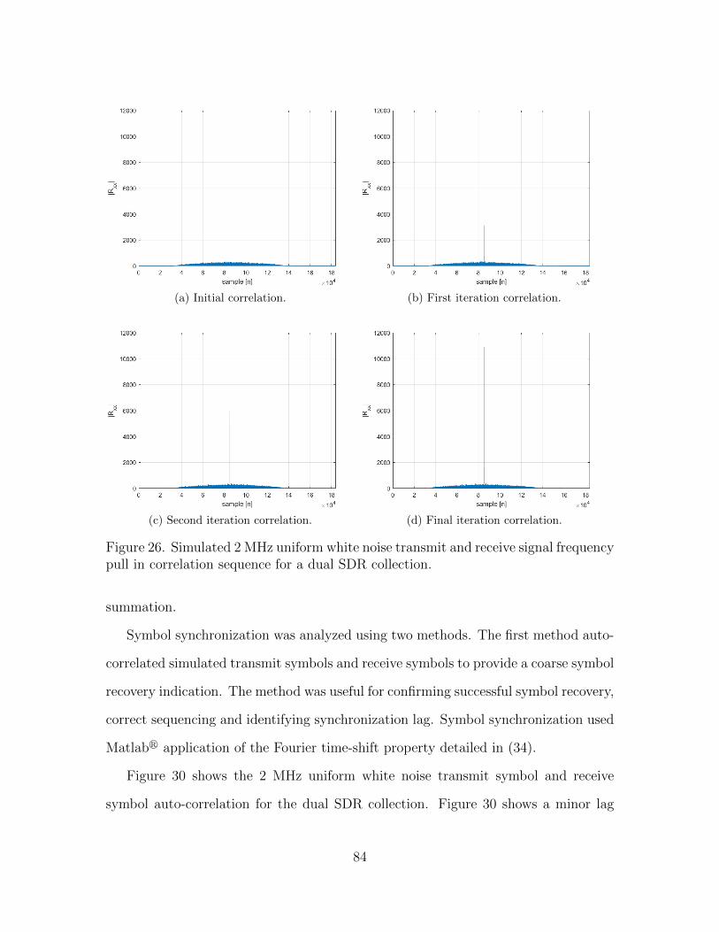
(a) Initial correlation. (b) First iteration correlation.
(c) Second iteration correlation. (d) Final iteration correlation.
Figure 26. Simulated 2 MHz uniform white noise transmit and receive signal frequencypull in correlation sequence for a dual SDR collection.
summation.
Symbol synchronization was analyzed using two methods. The first method auto-
correlated simulated transmit symbols and receive symbols to provide a coarse symbol
recovery indication. The method was useful for confirming successful symbol recovery,
correct sequencing and identifying synchronization lag. Symbol synchronization used
Matlabr application of the Fourier time-shift property detailed in (34).
Figure 30 shows the 2 MHz uniform white noise transmit symbol and receive
symbol auto-correlation for the dual SDR collection. Figure 30 shows a minor lag
84
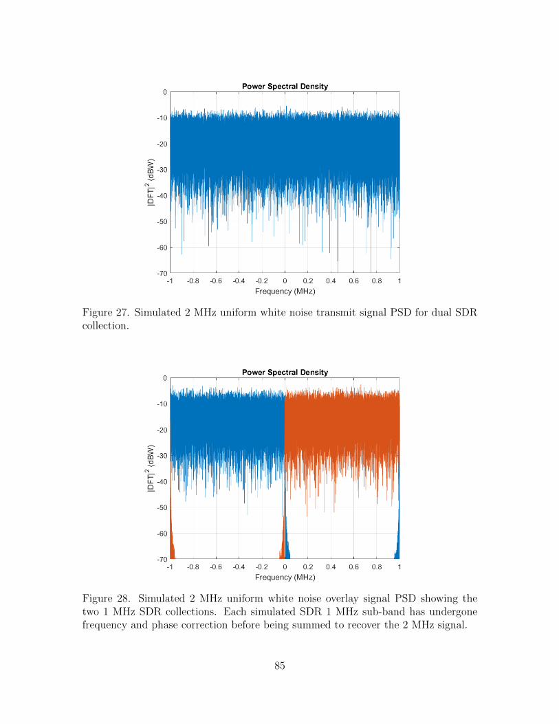
Figure 27. Simulated 2 MHz uniform white noise transmit signal PSD for dual SDRcollection.
Figure 28. Simulated 2 MHz uniform white noise overlay signal PSD showing thetwo 1 MHz SDR collections. Each simulated SDR 1 MHz sub-band has undergonefrequency and phase correction before being summed to recover the 2 MHz signal.
85
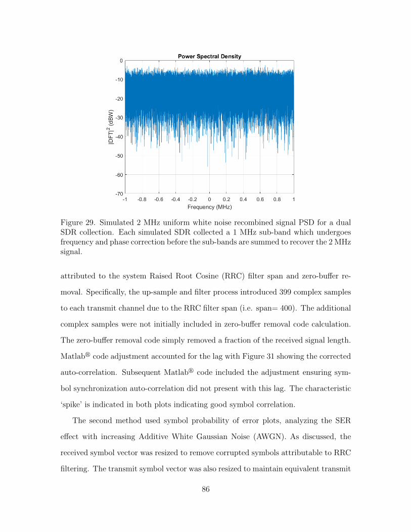
Figure 29. Simulated 2 MHz uniform white noise recombined signal PSD for a dualSDR collection. Each simulated SDR collected a 1 MHz sub-band which undergoesfrequency and phase correction before the sub-bands are summed to recover the 2 MHzsignal.
attributed to the system Raised Root Cosine (RRC) filter span and zero-buffer re-
moval. Specifically, the up-sample and filter process introduced 399 complex samples
to each transmit channel due to the RRC filter span (i.e. span= 400). The additional
complex samples were not initially included in zero-buffer removal code calculation.
The zero-buffer removal code simply removed a fraction of the received signal length.
Matlabr code adjustment accounted for the lag with Figure 31 showing the corrected
auto-correlation. Subsequent Matlabr code included the adjustment ensuring sym-
bol synchronization auto-correlation did not present with this lag. The characteristic
‘spike’ is indicated in both plots indicating good symbol correlation.
The second method used symbol probability of error plots, analyzing the SER
effect with increasing Additive White Gaussian Noise (AWGN). As discussed, the
received symbol vector was resized to remove corrupted symbols attributable to RRC
filtering. The transmit symbol vector was also resized to maintain equivalent transmit
86
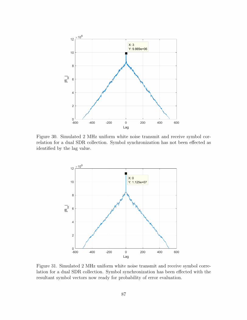
Figure 30. Simulated 2 MHz uniform white noise transmit and receive symbol cor-relation for a dual SDR collection. Symbol synchronization has not been effected asidentified by the lag value.
Figure 31. Simulated 2 MHz uniform white noise transmit and receive symbol corre-lation for a dual SDR collection. Symbol synchronization has been effected with theresultant symbol vectors now ready for probability of error evaluation.
87

and receive symbol vector lengths.
The Monte Carlo simulation SER versus Es/N0 plots are provided for the 2 MHz
uniform white noise signal. The Monte Carlo simulation was again conducted us-
ing 50 runs. The uniform white noise signal SER was compared with a theoretical
coherently detected M-ary orthogonal signal SER. The M-ary signal is sourced for
a bit value of k = 8, from [24]. The uniform white noise signal was also compared
with a simulated single-SDR, single-channel 2 MHz uniform white noise signal SER.
Figure 32 shows the simulated 2 MHz uniform white noise SER versus Es/N0, for a
dual SDR collection. An SER of 10−3 at an Es/N0 of 16 dB is indicated. There is a
3 dB loss between the simulated dual SDR collection SER and the theoretical M-ary
signal SER. A 0.5 dB loss is observed between the simulated dual SDR collection
SER and the simulated single SDR collection SER.
Figure 32. Monte Carlo simulation for the 2 MHz uniform white noise SER versusEs/N0 for 0 to 25 dB, for single and dual SDR collections.
88
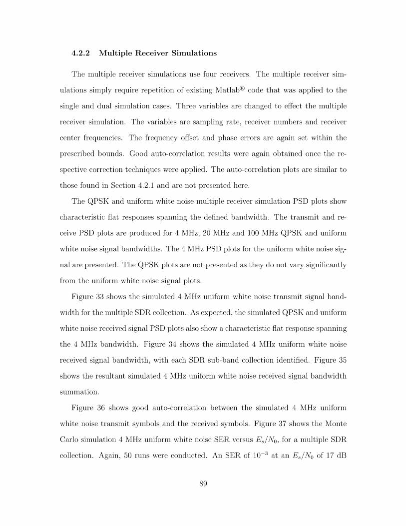
4.2.2 Multiple Receiver Simulations
The multiple receiver simulations use four receivers. The multiple receiver sim-
ulations simply require repetition of existing Matlabr code that was applied to the
single and dual simulation cases. Three variables are changed to effect the multiple
receiver simulation. The variables are sampling rate, receiver numbers and receiver
center frequencies. The frequency offset and phase errors are again set within the
prescribed bounds. Good auto-correlation results were again obtained once the re-
spective correction techniques were applied. The auto-correlation plots are similar to
those found in Section 4.2.1 and are not presented here.
The QPSK and uniform white noise multiple receiver simulation PSD plots show
characteristic flat responses spanning the defined bandwidth. The transmit and re-
ceive PSD plots are produced for 4 MHz, 20 MHz and 100 MHz QPSK and uniform
white noise signal bandwidths. The 4 MHz PSD plots for the uniform white noise sig-
nal are presented. The QPSK plots are not presented as they do not vary significantly
from the uniform white noise signal plots.
Figure 33 shows the simulated 4 MHz uniform white noise transmit signal band-
width for the multiple SDR collection. As expected, the simulated QPSK and uniform
white noise received signal PSD plots also show a characteristic flat response spanning
the 4 MHz bandwidth. Figure 34 shows the simulated 4 MHz uniform white noise
received signal bandwidth, with each SDR sub-band collection identified. Figure 35
shows the resultant simulated 4 MHz uniform white noise received signal bandwidth
summation.
Figure 36 shows good auto-correlation between the simulated 4 MHz uniform
white noise transmit symbols and the received symbols. Figure 37 shows the Monte
Carlo simulation 4 MHz uniform white noise SER versus Es/N0, for a multiple SDR
collection. Again, 50 runs were conducted. An SER of 10−3 at an Es/N0 of 17 dB
89

Figure 33. Simulated 4 MHz uniform white noise transmit signal PSD for multi-ple SDR collection.
Figure 34. Simulated 4 MHz uniform white noise overlay signal PSD showing thefour 1 MHz SDR collections. Each simulated SDR 1 MHz sub-band has undergonefrequency and phase correction before being summed to recover the 4 MHz signal.
90

Figure 35. Simulated 4 MHz uniform white noise recombined signal PSD for a mul-tiple (four) SDR collection. Each simulated SDR collected a 1 MHz sub-band whichundergoes frequency and phase correction before the sub-bands are summed to recoverthe 4 MHz signal.
is indicated. There is a 4 dB loss between the multiple SDR collection SER and the
theoretical M-ary signal SER, and a 1 dB loss between the simulated multiple SDR
collection SER and the simulated single SDR collection SER.
91
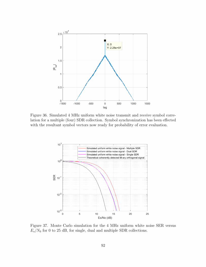
Figure 36. Simulated 4 MHz uniform white noise transmit and receive symbol corre-lation for a multiple (four) SDR collection. Symbol synchronization has been effectedwith the resultant symbol vectors now ready for probability of error evaluation.
Figure 37. Monte Carlo simulation for the 4 MHz uniform white noise SER versusEs/N0 for 0 to 25 dB, for single, dual and multiple SDR collections.
92
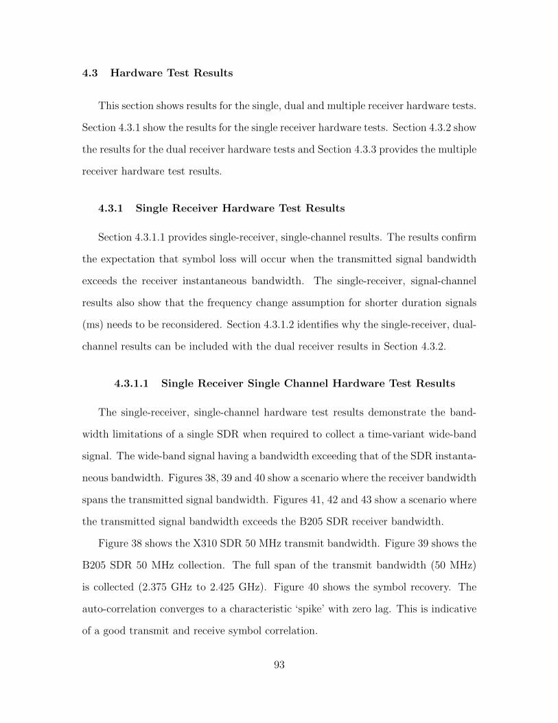
4.3 Hardware Test Results
This section shows results for the single, dual and multiple receiver hardware tests.
Section 4.3.1 show the results for the single receiver hardware tests. Section 4.3.2 show
the results for the dual receiver hardware tests and Section 4.3.3 provides the multiple
receiver hardware test results.
4.3.1 Single Receiver Hardware Test Results
Section 4.3.1.1 provides single-receiver, single-channel results. The results confirm
the expectation that symbol loss will occur when the transmitted signal bandwidth
exceeds the receiver instantaneous bandwidth. The single-receiver, signal-channel
results also show that the frequency change assumption for shorter duration signals
(ms) needs to be reconsidered. Section 4.3.1.2 identifies why the single-receiver, dual-
channel results can be included with the dual receiver results in Section 4.3.2.
4.3.1.1 Single Receiver Single Channel Hardware Test Results
The single-receiver, single-channel hardware test results demonstrate the band-
width limitations of a single SDR when required to collect a time-variant wide-band
signal. The wide-band signal having a bandwidth exceeding that of the SDR instanta-
neous bandwidth. Figures 38, 39 and 40 show a scenario where the receiver bandwidth
spans the transmitted signal bandwidth. Figures 41, 42 and 43 show a scenario where
the transmitted signal bandwidth exceeds the B205 SDR receiver bandwidth.
Figure 38 shows the X310 SDR 50 MHz transmit bandwidth. Figure 39 shows the
B205 SDR 50 MHz collection. The full span of the transmit bandwidth (50 MHz)
is collected (2.375 GHz to 2.425 GHz). Figure 40 shows the symbol recovery. The
auto-correlation converges to a characteristic ‘spike’ with zero lag. This is indicative
of a good transmit and receive symbol correlation.
93

Figure 38. Single receiver hardware test PSD showing an approximate 50 MHz (at−3 dB) transmit bandwidth.
Figure 39. Single receiver hardware test PSD showing an approximate 50 MHz (at−3 dB) collection bandwidth.
94
Figure 40. Single receiver hardware test plot showing a symbol recovery correlationfor the approximate 50 MHz (at −3 dB) collection bandwidth.
Figure 41 shows the X310 SDR 100 MHz transmit bandwidth. An attempt to
collect the transmitted signal using the GNU Radio Companion (GRC) with a B205
SDR receiver sampling rate set at 100 MS/s resulted in the GRC timing out. This was
expected. Reducing the receiver sampling rate to 50 MS/s resulted in the B205 SDR
collecting a 50 MHz bandwidth.
Figure 42 shows the B205 SDR 50 MHz collection (2.375 GHz to 2.425 GHz).
The full span of the transmit bandwidth cannot be collected (2.35 GHz to 2.45 GHz).
Figure 43 shows the symbol recovery. The convergence lacks the characteristic ‘spike’.
This is indicative of poor correlation. Accurate symbol recovery was not achieved.
Therefore, a wide-band signal exceeding the receiver instantaneous bandwidth will
not provide accurate symbol recovery using the above process. One solution is to
expand the usable bandwidth by introducing additional B205 SDRs.
In Section 3.2.1 an assumption was made that the frequency offset would be
constant for the short signal duration (ms) used in this research effort. Figure 44
95

Figure 41. Single receiver hardware test PSD showing an approximate 100 MHz (at−3 dB) transmit bandwidth.
Figure 42. Single receiver hardware test PSD showing the failed 100 MHz bandwidthcollection. Only an approximate 50 MHz (at −3 dB) bandwidth is collected due toB205 SDR bandwidth limitations.
96
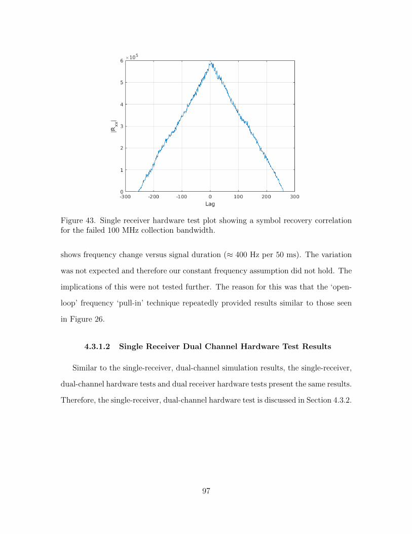
Figure 43. Single receiver hardware test plot showing a symbol recovery correlationfor the failed 100 MHz collection bandwidth.
shows frequency change versus signal duration (≈ 400 Hz per 50 ms). The variation
was not expected and therefore our constant frequency assumption did not hold. The
implications of this were not tested further. The reason for this was that the ‘open-
loop’ frequency ‘pull-in’ technique repeatedly provided results similar to those seen
in Figure 26.
4.3.1.2 Single Receiver Dual Channel Hardware Test Results
Similar to the single-receiver, dual-channel simulation results, the single-receiver,
dual-channel hardware tests and dual receiver hardware tests present the same results.
Therefore, the single-receiver, dual-channel hardware test is discussed in Section 4.3.2.
97

Figure 44. Hardware test frequency change versus signal duration for a uniform whitenoise single SDR collection.
98
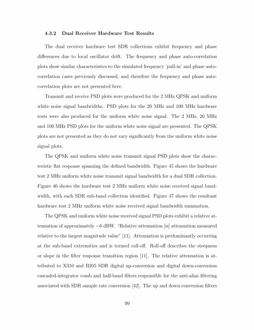
4.3.2 Dual Receiver Hardware Test Results
The dual receiver hardware test SDR collections exhibit frequency and phase
differences due to local oscillator drift. The frequency and phase auto-correlation
plots show similar characteristics to the simulated frequency ‘pull-in’ and phase auto-
correlation cases previously discussed, and therefore the frequency and phase auto-
correlation plots are not presented here.
Transmit and receive PSD plots were produced for the 2 MHz QPSK and uniform
white noise signal bandwidths. PSD plots for the 20 MHz and 100 MHz hardware
tests were also produced for the uniform white noise signal. The 2 MHz, 20 MHz
and 100 MHz PSD plots for the uniform white noise signal are presented. The QPSK
plots are not presented as they do not vary significantly from the uniform white noise
signal plots.
The QPSK and uniform white noise transmit signal PSD plots show the charac-
teristic flat response spanning the defined bandwidth. Figure 45 shows the hardware
test 2 MHz uniform white noise transmit signal bandwidth for a dual SDR collection.
Figure 46 shows the hardware test 2 MHz uniform white noise received signal band-
width, with each SDR sub-band collection identified. Figure 47 shows the resultant
hardware test 2 MHz uniform white noise received signal bandwidth summation.
The QPSK and uniform white noise received signal PSD plots exhibit a relative at-
tenuation of approximately −6 dBW. “Relative attenuation [is] attenuation measured
relative to the largest magnitude value” [11]. Attenuation is predominantly occurring
at the sub-band extremities and is termed roll-off. Roll-off describes the steepness
or slope in the filter response transition region [11]. The relative attenuation is at-
tributed to X310 and B205 SDR digital up-conversion and digital down-conversion
cascaded-integrator comb and half-band filters responsible for the anti-alias filtering
associated with SDR sample rate conversion [42]. The up and down-conversion filters
99

understandably lack the roll-off characteristics achievable in Matlabr software that
provided the PSD flat response seen in Figures 28 and 29. Roll-off of approximately
−3 dBW indicated at 0 MHz is attributed to B205 SDR cut-off filtering imposed by
receive bandwidth (sample rate) selection. It is hypothesized that sub-band overlap
could be used to reduce filter attenuation. This would require determining optimal
sub-band overlap and resolving overlap summation errors. Overlap considerations are
left as future work.
Figure 48 shows good auto-correlation between the hardware test 2 MHz uniform
white noise transmit and receive symbols. Symbol recovery for the hardware test
2 MHz uniform white noise recombined signal was accurate at the Es/N0 value in-
herent to each SDRs. Figure 49 shows the hardware test 2 MHz uniform white noise
SER versus Es/N0, for a dual SDR collection. For the hardware tests the SER re-
sults are a ‘best plot’ from a limited number of runs. An SER of 10−3 at an Es/N0
of 18 dB is indicated. There is a 5 dB loss between the dual SDR collection SER
and the theoretical M-ary signal SER, and 2 dB between the dual hardware test and
simulated single SDR collection SER.
The hardware test 2 MHz QPSK and uniform white noise signal dual SDR col-
lection were the first successful demonstrations of the auto-correlation bandwidth
technique. As discussed, the focus then moved to scaling the bandwidth. Figure 50
shows a hardware test 20 MHz uniform white noise recombined signal PSD for a dual
SDR collection. This was the widest bandwidth tested with the 1 Gigabit Ethernet
(1G ETH) connection. This was due to the aforementioned usable bandwidth and
X310 sampling rate decimation requirements.
Figure 51 shows the 100 MHz uniform white noise recombined signal PSD for
a dual SDR collection. This recovery required 10 Gigabit Ethernet (10G ETH).
A 100 MHz bandwidth was the widest bandwidth tested. Figure 52 shows symbol
100
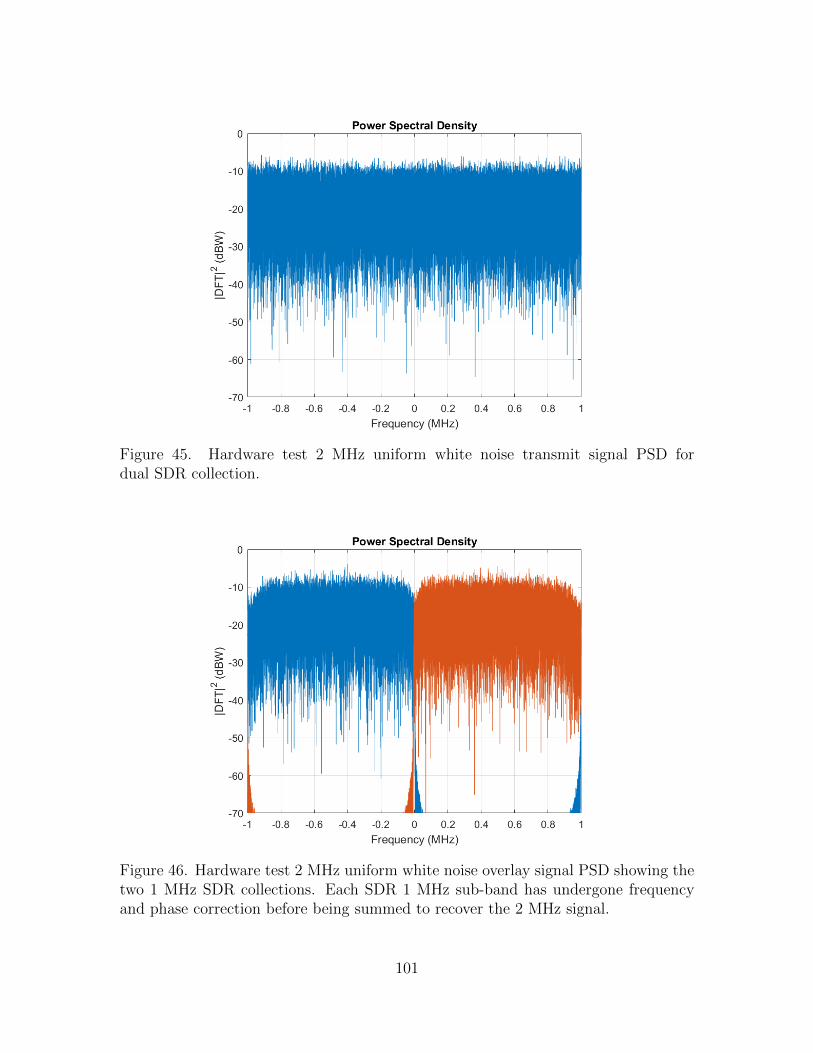
Figure 45. Hardware test 2 MHz uniform white noise transmit signal PSD fordual SDR collection.
Figure 46. Hardware test 2 MHz uniform white noise overlay signal PSD showing thetwo 1 MHz SDR collections. Each SDR 1 MHz sub-band has undergone frequencyand phase correction before being summed to recover the 2 MHz signal.
101
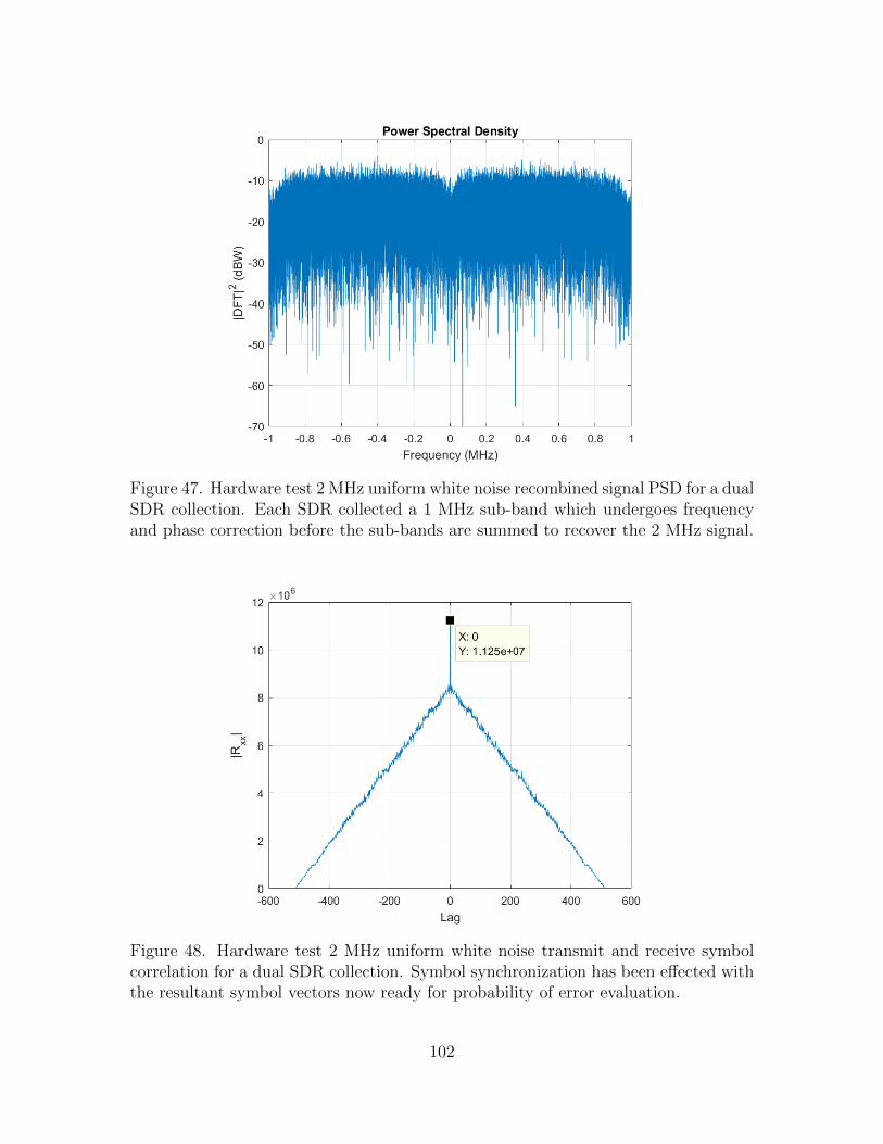
Figure 47. Hardware test 2 MHz uniform white noise recombined signal PSD for a dualSDR collection. Each SDR collected a 1 MHz sub-band which undergoes frequencyand phase correction before the sub-bands are summed to recover the 2 MHz signal.
Figure 48. Hardware test 2 MHz uniform white noise transmit and receive symbolcorrelation for a dual SDR collection. Symbol synchronization has been effected withthe resultant symbol vectors now ready for probability of error evaluation.
102

Figure 49. Hardware test 2 MHz uniform white noise SER versus Es/N0 for 0 to 25 dB,for a dual SDR collection.
recovery for the hardware test 100 MHz uniform white noise recombined signal is
accurate at the Es/N0 value inherent to each SDRs.
Two interesting points arise from the 100 MHz hardware test. First, the PSD roll-
off at 0 MHz is approximately −6 dBW. This is attributed to X310 and B205 SDR
digital up-conversion and digital down-conversion cascaded-integrator comb and half-
band filters responsible for anti-alias filtering associated with SDR sample rate con-
version. The roll-off of approximately −3 dBW previously indicated at 0 MHz due to
B205 SDR cut-off filtering is no longer dominant. Second, the use of 10G ETH caused
GRC to display an underrun (‘U ’) condition. This is interpreted as the host-PC not
producing data packets fast enough for the SDR. This issue was resolved by looping
the transmit signal in the GRC.
103
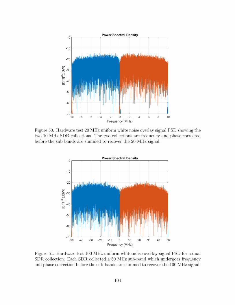
Figure 50. Hardware test 20 MHz uniform white noise overlay signal PSD showing thetwo 10 MHz SDR collections. The two collections are frequency and phase correctedbefore the sub-bands are summed to recover the 20 MHz signal.
Figure 51. Hardware test 100 MHz uniform white noise overlay signal PSD for a dualSDR collection. Each SDR collected a 50 MHz sub-band which undergoes frequencyand phase correction before the sub-bands are summed to recover the 100 MHz signal.
104

Figure 52. Hardware test 100 MHz uniform white noise transmit and receive symbolcorrelation for a dual SDR collection. The symbol synchronization shows that wide-band signal reconstruction exceeding a single B205 SDR instantaneous bandwidth ispossible using the techniques described in this research effort.
105

4.3.3 Multiple Receiver Hardware Test Results
The multiple receiver hardware tests use four B205 SDR receivers. The SDR
collections exhibit frequency and phase differences due to local oscillator drift. Fre-
quency ‘pull-in’ auto-correlation plots are similar to those shown for the dual re-
ceiver hardware tests, and therefore frequency auto-correlation plots are not pre-
sented here. Again, phase auto-correlation plots show similar characteristics to the
frequency pull-in plot for both the uncorrelated and correlated cases, and therefore
phase auto-correlation plots are not presented here.
Transmit and receive PSD plots were produced for 4 MHz QPSK and uniform
white noise signal bandwidths. 20 MHz and 100 MHz were also produced for the
uniform white noise signal. The 4 MHz, 20 MHz and 100 MHz PSD plots for the
uniform white noise signal are presented. 4 MHz QPSK plots are also presented.
The QPSK and uniform white noise transmit signal PSD plots show the charac-
teristic flat response spanning the defined bandwidth. Figure 53 shows the 4 MHz
uniform white noise transmit signal bandwidth for a multiple SDR collection. Fig-
ure 54 shows the 4 MHz uniform white noise receive signal bandwidth for the multiple
SDR collection, with each SDR sub-band collection identified. Figure 55 shows the
resultant 4 MHz uniform white noise receive signal bandwidth summation for the
multiple SDR collection.
Similar to the dual SDR collections, PSD plots for QPSK and uniform white
noise tests show a relative attenuation of −6 dBW, predominantly at SDR sub-band
extremities. This is attributed to X310 and B205 SDR in-built signal filtering, as
described in Section 4.3.2.
Figure 56 shows the hardware test 4 MHz QPSK recombined signal PSD for the
multiple SDR collection. RxC exhibits a 10 dBW loss. The issue was corrected by
increasing SDR receiver gain. Figure 57 shows the hardware test 4 MHz QPSK recom-
106

Figure 53. Hardware test 4 MHz uniform white noise transmit signal PSD for multi-ple SDR collection.
bined signal PSD for the multiple SDR collection, with the receiver gain corrected.
GRC receiver gain settings contributed significantly to result variation in early QPSK
single, dual and four receiver hardware tests. Gain settings were selected after much
trial and error, and was dependent, not only on the hardware test, but time-varying
factors such as receiver temperature or cable connection quality. The receiver gain
issue was not apparent during uniform white noise receiver tests.
Figure 58 shows good auto-correlation between hardware test 4 MHz uniform
white noise transmit and received symbols for the multiple SDR collection. Symbol
recovery for the hardware test 4 MHz uniform white noise recombined signal was
accurate at the Es/N0 value inherent to each SDRs. Figure 59 shows the hardware
test 4 MHz uniform white noise SER versus Es/N0, for a multiple SDR collection. For
the hardware tests the SER results are a ‘best plot’ from a limited number of runs.
An SER of 10−3 at an Es/N0 of 19 dB is indicated. There is a 6 dB loss between the
multiple SDR collection SER and the theoretical M-ary signal SER, and a 3 dB loss
107

Figure 54. Hardware test 4 MHz uniform white noise overlay signal PSD showing thefour 1 MHz SDR collections. Each SDR 1 MHz sub-band has undergone frequencyand phase correction before being summed to recover the 4 MHz signal.
Figure 55. Hardware test 4 MHz uniform white noise recombined signal PSD fora multiple SDR collection. Each SDR collected a 1 MHz sub-band which undergoesfrequency and phase correction before the sub-bands are summed to recover the 4 MHzsignal.
108

Figure 56. Hardware test 4 MHz QPSK overlay signal for a multiple SDR collection.Each SDR collected a 1 MHz sub-band which undergoes frequency and phase correc-tion before the sub-bands are summed to recover the 4 MHz signal. Receiver gainsettings require adjustment to correct the power loss in ‘RxC ’.
Figure 57. Hardware test 4 MHz QPSK overlay signal showing the four 1 MHz SDRcollections. Receiver gain settings for all receivers have been increased. The powerloss issue with ‘RxC ’ is no longer apparent.
109
between the multiple SDR collection SER and the simulated single SDR collection
SER.
The 4 MHz hardware test was the first successful demonstration of the auto-
correlation bandwidth technique using multiple receivers. The focus shifted to in-
creasing single SDR bandwidth use, followed by bandwidth recovery exceeding single
SDR instantaneous bandwidth limits. Again, a simple sampling rate adjustment
and center frequency recalculation for each sub-band were the only variable changes
required to extend recoverable bandwidth limits.
As with the dual SDR recovery, as long as sampling rate settings were consistent
with X310 SDR sample rate decimation requirements and the 1G ETH bit-rate was
not exceeded, bandwidth recovery could be extended to 20 MHz. Figure 60 shows
a hardware test 20 MHz uniform white noise recombined signal for a multiple SDR
collection. This is the widest bandwidth tested with the 1G ETH connection. Symbol
recovery for the hardware test 20 MHz uniform white noise recombined signal is
accurate at the Es/N0 value inherent to each SDRs.
Figure 61 shows the 100 MHz uniform white noise recombined signal PSD for
a multiple SDR recovery. Figure 62 shows symbol recovery for the hardware test
100 MHz uniform white noise recombined signal is accurate at the Es/N0 value in-
herent to each SDRs. A 100 MHz bandwidth was the widest bandwidth tested for
the multiple SDR receiver case.
110
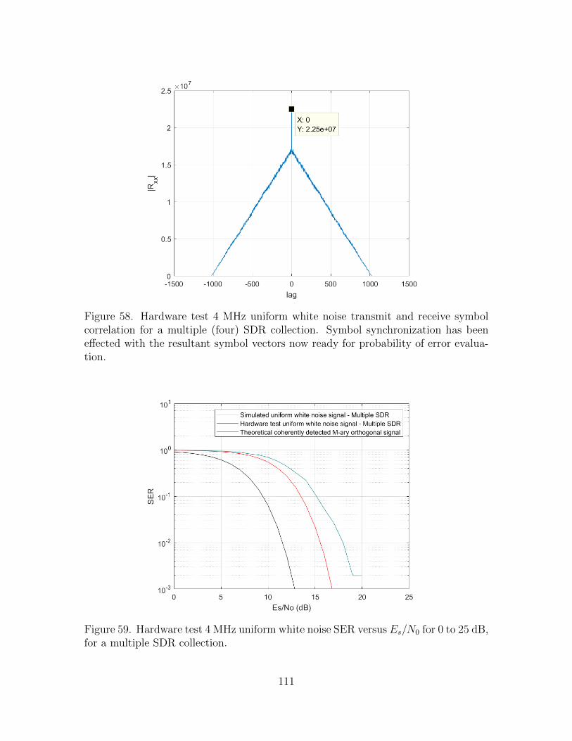
Figure 58. Hardware test 4 MHz uniform white noise transmit and receive symbolcorrelation for a multiple (four) SDR collection. Symbol synchronization has beeneffected with the resultant symbol vectors now ready for probability of error evalua-tion.
Figure 59. Hardware test 4 MHz uniform white noise SER versus Es/N0 for 0 to 25 dB,for a multiple SDR collection.
111
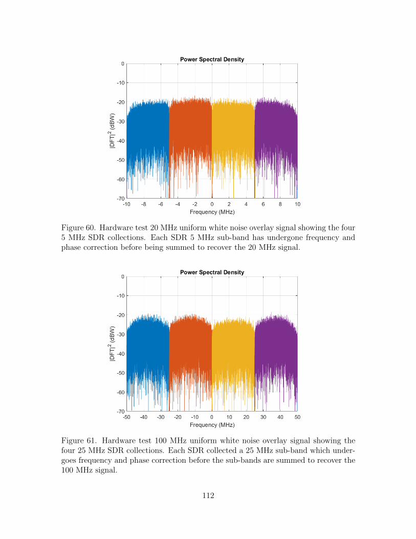
Figure 60. Hardware test 20 MHz uniform white noise overlay signal showing the four5 MHz SDR collections. Each SDR 5 MHz sub-band has undergone frequency andphase correction before being summed to recover the 20 MHz signal.
Figure 61. Hardware test 100 MHz uniform white noise overlay signal showing thefour 25 MHz SDR collections. Each SDR collected a 25 MHz sub-band which under-goes frequency and phase correction before the sub-bands are summed to recover the100 MHz signal.
112

Figure 62. Hardware test 100 MHz uniform white noise transmit and receive symbolcorrelation for a multiple (four) SDR collection. The symbol synchronization showsthat wide-band signal reconstruction exceeding a single B205 SDR instantaneousbandwidth is possible using the techniques described in this research effort.
4.4 RFDNA Test Results
The intent of the RF-DNA test case was to demonstrate a real-world application
for the auto-correlation bandwidth expansion technique. However, the proposed RF-
DNA test was not conducted and is left as future work.
4.5 Summary
Chapter IV detailed research effort results and analysis. The results show that a
uniform white noise transmit signal, with a bandwidth exceeding a single B205 SDR
instantaneous bandwidth, can be simultaneously collected and reconstructed using
multiple SDRs and the described auto-correlation bandwidth expansion technique.
The auto-correlation technique requires no overlap of the collected sub-bands. PSD
plots for single, dual and multiple SDR receiver simulations and hardware tests for
113

transmit bandwidths of 2 MHz, 4 MHz, 20 MHz and 100 MHz demonstrate the
technique is scalable.
The research culminates with two 100 MHz bandwidth hardware tests. The two
uniform white noise hardware tests use a two B205 SDR and a four B205 SDR collec-
tion. Symbol recovery for the two hardware tests were accurate at the Es/N0 value
inherent to each SDRs. Chapter V will provide research effort conclusions and future
work recommendations.
114
V. Conclusion
The research objective was to demonstrate wide-band signal response collection si-
multaneously spanning multiple Software Defined Radio (SDR) narrow-band receiver
bandwidths using a uniform white noise signal. The simultaneous collections were
then recombined to provide a wide-band receive signal. The receive signal was then
demodulated to provide accurate symbol recovery. This objective had two require-
ments:
• A hardware test should be developed to demonstrate collection and reconstruc-
tion of a signal bandwidth exceeding that of an individual SDR instantaneous
bandwidth.
• A hardware test should be developed to demonstrate collection and reconstruc-
tion of a signal using multiple SDRs.
An additional objective was to determine the minimum number of SDRs required to
collect the full span of a transmit signal bandwidth.
The initial attempts to develop hardware tests using Everett’s cross-correlation
techniques met with some difficulty [8]. While always intending to substitute a uni-
form white noise signal for the Quadrature Phase Shift Keying (QPSK) signal, a
successful outcome would have provided a useful baseline for further bandwidth ex-
pansion development. The full replication of Everett’s technique was ultimately aban-
doned in favor of an alternate approach. The alternate approach used auto-correlation
to exploit a known a priori transmit signal.
As seen, in Chapter IV, the auto-correlation technique was able to recover the
uniform white noise signal. Indeed, while this research effort did not achieve all
the objectives, there were three significant outcomes that progress Non-Destructive
Evaluation (NDE) system development. These outcomes were:
115

• The successful simulation and hardware testing of an auto-correlation band-
width expansion technique using dual and multiple B205 SDRs to collect and
restore a uniform white noise signal with a bandwidth of 100 MHz. This band-
width is greater than the instantaneous bandwidth of the B205 SDR. Previous
research efforts used two SDRs to recover a 1.98 MHz bandwidth from a 2 MHz
QPSK signal.
• The successful simulation and hardware testing of an auto-correlation band-
width expansion technique for simultaneous collection and reconstruction of
QPSK or uniform white noise signals, using more than two SDRs.
• The successful development and application of a uniform white noise signal
comprised of complex symbols, drawn randomly without replacement. Previous
research efforts used communication-centric signals (e.g. QPSK). This outcome
demonstrated noise signals similar to that generated by the Air Force Institute
of Technology (AFIT) Noise Radar Network (NoNET) could be recovered by
light-weight, low-cost and low-complexity SDRs.
One further issue raised as future work in [8] was resolved during this research
effort. The issue required transmit spike elimination. As discussed, the transmit spike
presented if a DC bias was coded into the transmit signal. Offsetting complex symbol
inputs so both real and imaginary values were uniformly distributed with zero mean
eliminated the observed transmit spike.
This research effort restricted overlap to that part of the bandwidth extending
beyond the pass-band cut-off frequency. The bandwidth expansion auto-correlation
technique is therefore optimized for equation (29). Further, the minimal code changes
required to transition from a dual to multiple SDR collection suggests the technique
is scalable.
116

5.1 Future Work
Due to difficulties with the modelling process, the XTRX SDR bandwidth expan-
sion technique transfer was not investigated. The intended Radio Frequency-Distinct
Native Attribute (RF-DNA) test was also not conducted. Additionally, the extent
of intended bandwidth expansion was limited by hardware restrictions and sampling
considerations, primarily due to host-PC and SDR analog bandwidth restrictions. A
further hardware consideration is the effect of SDR filter attenuation. Consequently,
there is still further work to do.
5.1.1 Bandwidth Expansion Technique Transfer
To confirm whether the auto-correlation bandwidth expansion technique devel-
oped in this research effort is transferable, it is recommended that the auto-correlation
bandwidth expansion technique be tested using alternate SDR hardware. A trans-
ferable process would allow future NDE hardware to be tailored to user needs. The
Fairwaves XTRX and Blade RF SDRs are suggested as suitable alternatives for this
work.
5.1.2 Alternate Support Hardware Tests
The constraints imposed on sampling rates by the low-complexity Universal Soft-
ware Radio Peripheral (USRP) devices and the bit-rates supported by 1 Gigabit
Ethernet (1G ETH) restricted bandwidth expansion to approximately 20 MHz. Ex-
pansion beyond this limit, and dependent on sample rate interpolation and decima-
tion settings sometimes within this limit, caused buffer overflow ‘O’ conditions. While
B205 SDR documentation noted that buffer overflow is “generally harmless” this was
not the case for hardware tests [40].
Alternative host-PC hardware and 10 Gigabit Ethernet (10G ETH) with pro-
117

cessing capability sufficient to support wider instantaneous bandwidth data transfer
still restricted tests to a 100 MHz transmit signal bandwidth. Sourcing a host-PC,
and commercial-off-the-shelf portable transmit hardware able to support the NoNET
bandwidth (395− 720 MHz) is necessary to further auto-correlation bandwidth tech-
nique investigation.
5.1.3 SDR Filter Attenuation
Figures 46, 47, 54 and 55 show the attenuation attributed to SDR transmitter
and receiver in-built filters. Losses due to filtering need to be quantified. A proposed
hypothesis is that the EsNo degradation experienced during this research effort is
in part attributable to the filters. If the losses are significant, a bandwidth overlap
process could be developed to reduce filter attenuation effects and create a contiguous
flat bandwidth response. This would have implications for equation (29). Increasing
overlap would require an increasing number of receivers to span the same wide-band
transmit signal bandwidth. Comparative tests to optimize the number of receivers
versus the required bandwidth overlap could then be conducted.
5.1.4 RF-DNA Tests
The intended RF-DNA hardware test did not occur. This was unfortunate as a
RF-DNA test provides an NDE of a Device Under Test (DUT). A successful NDE test
would show the real-world application of the auto-correlation bandwidth expansion
technique. A successful test would also provide further cases of uniform white noise
signal use in the RF-DNA field.
118

Appendix A: Non-Linear Least Squares Estimation
The estimate aims to provide the best possible solution for a non-linear system.
The proof, found in [26], is repeated here with additional equations and explanation
for completeness. Despite the insertion of additional equations and explanation, this
appendix is not claimed as independent work. The equations and a large portion of
the text are copied from [26]. The proof begins with a statement of the Non-Linear
Least Squares (NLS) criteria for (38),
minα,ω,x
||y − αDx||2, (38)
where y = [y(0), y(1), ...y(N −1)]T , x = [x(0), x(1), ...x(N −1)T ], D = diag(1, ejω, ...,
ej(N−1)ω), N is the number of samples and T is the transpose operator, with α being
the least squares solution [26]. Minimizing the sum of squares (38) is the same as
minimizing (39),
minα,ω,x
(y − αDx), (39)
To minimize (39) identification of the normal equation is required. The normal equa-
tion is (40),
xT ((y − αDx) = 0, (40)
where xT indicates the transpose of x [26]. Expanding (40) rearranging and isolating
for α provides (41), (42) and (43),
xTy − xTαDx = 0, (41)
xTy = xTαDx, (42)
119
α = xTD∗y/xTx, (43)
where ∗ indicates the complex conjugate [26]. Substituting (43) in (42) provides a
solution for minimizing α (44),
minω,x||(I −DxxTD∗/xTx)y||2, (44)
which equates to maximizing (45),
y∗DxxTD∗y/xTx = |xT z|2/xTx, (45)
where z = D∗y is a function of ω [26]. To maximize (45) with respect to x ∈ <N×1,
let,
z = zr + izi, (46)
and observe that,
|xT z|2 = (xT zr)2 + (xT zi)
2 = xT [zr zi]
zTrzTi
x = xTZZTx, (47)
Next let,
ZTZ = U
λ1 0
0 λ2
UT = UΛUT , (48)
denote the eigenvalue decomposition of the 2 × 2 matrix ZTZ where λ1 ≥ λ2 and
U = [u1 u2] is an orthogonal matrix [26]. Note that generically we have λ1 > λ2,
which we assume in the following. A simple calculation shows that,
120
(ZZT )× Z(ZTZ)−1/2U︸ ︷︷ ︸V
= Z(ZTZ)1/2U
= Z(ZTZ)−1/2U × UT (ZTZ)U︸ ︷︷ ︸Λ
= V Λ,
(49)
where (.)1/2 denotes the square root of the matrix between parentheses [26]. The
N × N matrix ZZT has N − 2 eigenvalues equal to zero. It follows from (49) that
the other two eigenvalues of ZZT are equal to λ1, λ2 and, also, that the eigenvector
associated with λ1 is given by,
v1 = Z(ZTZ)−1/2u1), (50)
Since we have assumed that ||x|| = 1, it follows that the maximum of the function in
(45),(47) with respect to x is obtained for
x = v1, (51)
and that,
ω = arg maxω
λ1(ω), (52)
A closed-form expression for λ1(ω) can be readily obtained as,
zTr zr − λ zTr zi
zTr zi zTi zi − λ
= λ2 − λ(zTr zr + zTi zi) + (zTr zr)(zTi zi)− (zTr zi)
2, (53)
we obtain,
2λ1 = (zTr zr + zTi zi) + [(zTr zr − zTi zi)2 + 4(zTr zi)2]1/2, (54)
121

Now,
zTr zr + zTi zi = z∗z, (55)
(zTr zr − ZTi zi)
2 + 4(zTr zi)2 = |zT z|2, (56)
Hence, ω0 is obtained by maximizing,
z∗z + |zT z|, (57)
Since z∗z does not depend on ω, it follows that the NLS frequency estimate is given
by,
ω0 = arg maxω
1
N
∣∣∣∣∣N−1∑n=0
y2(n)e−j2ωn
∣∣∣∣∣2
, (58)
This completes the proof.
122
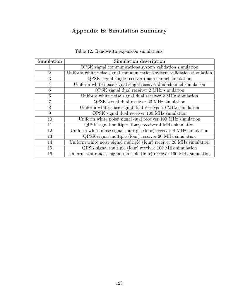
Appendix B: Simulation Summary
Table 12. Bandwidth expansion simulations.
Simulation Simulation description1 QPSK signal communications system validation simulation2 Uniform white noise signal communications system validation simulation3 QPSK signal single receiver dual-channel simulation4 Uniform white noise signal single receiver dual-channel simulation5 QPSK signal dual receiver 2 MHz simulation6 Uniform white noise signal dual receiver 2 MHz simulation7 QPSK signal dual receiver 20 MHz simulation8 Uniform white noise signal dual receiver 20 MHz simulation9 QPSK signal dual receiver 100 MHz simulation10 Uniform white noise signal dual receiver 100 MHz simulation11 QPSK signal multiple (four) receiver 4 MHz simulation12 Uniform white noise signal multiple (four) receiver 4 MHz simulation13 QPSK signal multiple (four) receiver 20 MHz simulation14 Uniform white noise signal multiple (four) receiver 20 MHz simulation15 QPSK signal multiple (four) receiver 100 MHz simulation16 Uniform white noise signal multiple (four) receiver 100 MHz simulation
123

Appendix C: Hardware Test Summary
Table 13. Bandwidth expansion hardware tests.
Hardware test Hardware test description1 Single SDR receiver hardware test using
a 2 MHz QPSK transmission signal2 Single SDR receiver hardware test using a 2 MHz uniform
white noise transmission signal3 Dual SDR receiver hardware test using a 2 MHz QPSK
transmission signal4 Dual SDR receiver hardware test using a 2 MHz uniform
white noise transmission signal5 Dual SDR receiver hardware test using a 20 MHz uniform
white noise transmission signal6 Dual SDR receiver hardware test using a 100 MHz uniform
white noise transmission signal7 Multiple (four) SDR receiver hardware test using a 4 MHz QPSK
transmission signal8 Multiple (four) SDR receiver hardware test using a 4 MHz uniform
white noise transmission signal9 Multiple (four) SDR receiver hardware test using a 20 MHz uniform
white noise transmission signal10 Multiple (four) SDR receiver hardware test using a 100 MHz uniform
white noise transmission signal
124

Bibliography
1. R. C. McMaster, Nondestructive Testing Handbook, Vol 1. The Ronald Press
Company, New York, NY, 1959.
2. M. W. Lukacs, P. J. Collins, and M. A. Temple, “Interrogation Signal Optimiza-
tion for Improved Classifier Performance when using for Non-Destructive Antenna
Acceptance Testing,” Proceedings of the Antenna Measurement Techniques As-
sociation 37th Annual Symposium, pp. 1–6, 2015.
3. M. W. Lukacs, P. J. Collins, and M. A. Temple, ““RF-DNA” Fingerprinting for
Non-Destructive Antenna Acceptance Testing,” Proceedings of the Antenna Mea-
surement Techniques Association 36th Annual Symposium, pp. 314–319, 2014.
4. M. W. Lukacs, A. J. Zeqolari, P. J. Collins, and M. A. Temple, “RF-DNA Finger-
printing for Antenna Classification,” IEEE Antennas and Wireless Propagation
Letters, 2015.
5. M. A. Temple, P. J. Collins, and M. W. Lukacs, “Classification performance using
’RF-DNA’ fingerprinting of ultra-wideband noise waveforms,” Electronics Letters,
vol. 51, no. 10, pp. 787–789, 2015.
6. M. W. Lukacs, P. J. Collins, and M. A. Temple, “Device Identification Using
Active Noise Interrogation and RF-DNA Fingerprinting for Non-Destructive
Amplifier Acceptance Testing,” 2016 IEEE 17th Annual Wireless and Microwave
Technology Conference (WAMICON), pp. 1–6, 2016.
7. A. J. Paul, P. J. Collins, and M. A. Temple, “Nondestructive Evaluation of Ra-
dio Frequency Connector Continuity Using Stimulated Emissions,” Journal of
Nondestructive Evaluation, Diagnostics and Prognostics of Engineering Systems,
vol. 2, no. 1, p. 011010, 2018.
125

8. N. Everett, “Instantaneous bandwidth expansion using software defined radios,”
Master’s thesis, Air Force Institute of Technology, 2019.
9. B. Stewart, K. Barlee, D. Atkinson, and L. Crockett, Software Defined Radio
using MATLAB and Simulink and the RTL-SDR. Strathclyde Academic Media,
Ltd., G43 2DX Glasgow, UK, 2015.
10. “Ettus Research USRP B205 mini Software Defined Radio [Product Datasheet],”
Ettus Resarch, National Instruments, Santa Clara, CA, 2010.
11. R. G. Lyons, Understanding Digital Signal Processing, Second Edition. Pearson
Education Inc., Upper Saddle River, NJ, 2004.
12. S. L. Miller and D. Childers, Probability and Random Processes, Second Edition.
Academic Press, Waltham, MA, 2012.
13. J. Hardin, “Information encoding on a pseudo random noise radar waveform,”
Master’s thesis, Air Force Institute of Technology, 2013.
14. P. J. Collins and J. A. Priestly, “Trading spectral efficiency for system latency
in true-random noise radar network through template-replay diversity,” 2012
International Waveform Diversity & Design Conference (WDD), pp. 238–242,
2012.
15. A. Hauser, B. Fenski, and L. Cavalli, “Maximize Asset Availability and Reduce
Maintenance Costs - an Integrated Approach Combining Conditon Assessment
with Data Analytics,” 24th International Conference & Exhibition on Electricity
Distribution (CIRED), pp. 316–319, 2017.
16. “RF Agile Transceiver AD9364 [Product Datasheet],” Analog Devices, Norwood,
MA, 2014.
126
17. “Ettus Research USRP X310 Software Defined Radio [Product Datasheet],” Ettus
Resarch, National Instruments, Santa Clara, CA, 2010.
18. “GNU Radio,” The GNU Radio Foundation, Inc., The Free Software Foundation,
Boston, MA, 2020.
19. J. S. Beasley and G. M. Miller, Modern Electronic Communication, Ninth Edition.
Pearson Education Inc., Upper Saddle River, NJ, 2008.
20. E. Zenteno, M. Isaksson, and P. Handel, “Pilot tone aided measurements to
extend the bandwidth of radio frequency applications,” Measurement: Journal of
the International Measurement Confederation, vol. 90, pp. 534–541, 2016.
21. D. Wisell, D. Ronnow, and P. Handel, “A Technique to Extend the Bandwidth of
an RF Power Amplifier Test Bed,” IEEE Transactions on Instrumentation and
Measurement, vol. 56, no. 4, pp. 1488–1494, 2007.
22. K. A. Remley, D. F. Williams, D. M. Schreurs, L. Giovanni, and A. Cidronal,
“Phase Detrending for Measured Multisine Signals *,” In: 61st ARFTG Confer-
ence Digest Spring 2003, pp. 73–83, 2003.
23. E. D. Kaplan and C. J. Hegarty, Understanding GPS Principles and Applications,
Second Edition. Artech House, Inc., Norwood, MA, 2006.
24. B. Sklar, Digital Communications Fundamentals and Applications, Second Edi-
tion. Prentice Hall Inc., Upper Saddle River, NJ, 2001.
25. D. Sorensen, C. Lindstrom, and J. Gunther, “Exponent: Arbitrary Bandwidth
Receiver Architecture,” Proceedings of the GNU Radio Conference, vol. 4, no. 1,
2019.
127
26. O. Besson and P. Stoica, “Frequency estimation and detection for sinusoidal sig-
nals with arbitrary envelope: a nonlinear least-squares approach,” Digital Signal
Processing, vol. 56, no. 1999, pp. 2209–2212, 2002.
27. Y. Wang, K. Shi, and E. Serpedin, “Non-Data-Aided Feed-Forward Carrier Fre-
quency Offset Estimators for QAM Constellations: A Non-Linear Least-Squares
Approach,” Eurasip Journal on Applied Signal Processing, vol. 2004, no. 13,
pp. 1993–2001, 2004.
28. U. Mengali and M. Morelli, “Data-Aided Frequency Estimation for Burst Digital
Transmission,” IEEE Transactions on Communication, vol. 45, no. 1, pp. 23–25,
1997.
29. J. G. Proakis, Digital Communications, Third Edition. McGraw Hill., New York,
NY, 1995.
30. B. P. Lathi and Z. Ding, Modern Digital and Analog Communication Systems,
Fourth Edition. Oxford University Press., New York, NY, 2009.
31. R. W. Klein, M. A. Temple, and M. J. Mendenhall, “Application of Wavelet-
Based RF Fingerprinting to Enhance Wireless Network Security,” Journal of
Communications and Networks, vol. 11, no. 6, pp. 544–555, 2009.
32. C. K. Dubendorfer, B. W. Ramsey, and M. A. Temple, “An RF-DNA Verifica-
tion Process for ZigBee Networks,” Proceedings - IEEE Military Communications
Conference MILCOM, pp. 1–6, 2012.
33. D. R. Reising, M. A. Temple, and J. A. Jackson, “Authorized and Rogue De-
vice Discrimination Using Dimensionally Reduced RF-DNA Fingerprints,” IEEE
Transactions on Information Forensics and Security, vol. 10, no. 6, pp. 1180–
1192, 2015.
128

34. P. E. Pace, Detecting and Classifying Low Probability of Intercept Radar. Artech
House Inc., Norwood, MA, 2004.
35. M. A. Richards, J. A. Scheer, and W. A. Holm, Principles of Modern Radar,
Basic Principles. SciTech Publishing, Raileigh, NC, 2010.
36. C. M. Talbot, M. A. Temple, T. J. Carbino, and J. A. Betances, “Detecting
Rogue Attacks on Commercial Wireless Insteon Home Automation Systems,”
Computers and Security, vol. 74, pp. 296–307, 2018.
37. D. R. Reising, M. A. Temple, and M. J. Mendenhall, “Improving Intra-cellular
Security using Air Monitoring with Radio Frequency (RF) Fingerprints,” IEEE
Wireless Communications and Networking Conference, pp. 1–6, 2015.
38. R. O. Duda, P. E. Hart, and D. G. Stork, Pattern Classification, Second Edition.
John Wiley & Sons, Inc., New York, NY, 2001.
39. D. C. Montgomery, Design and Analysis of Experiments, Ninth Edition. John
Wiley & Sons, Inc., Hoboken, NJ, 2017.
40. “Ettus Research USRP B205 mini Software Defined Radio [User Manual],” Ettus
Resarch, National Instruments, Santa Clara, CA, 2010.
41. “Agilent 33250A 80 MHz Function/Arbitrary Waveform Generator [User Guide]
Ed. 2.,” Agilent Technologies, Santa Clara, CA, 2003.
42. “About USRP Bandwidths and Sampling Rates [Application Note 177],” Ettus
Resarch, National Instruments, Santa Clara, CA, 2016.
129
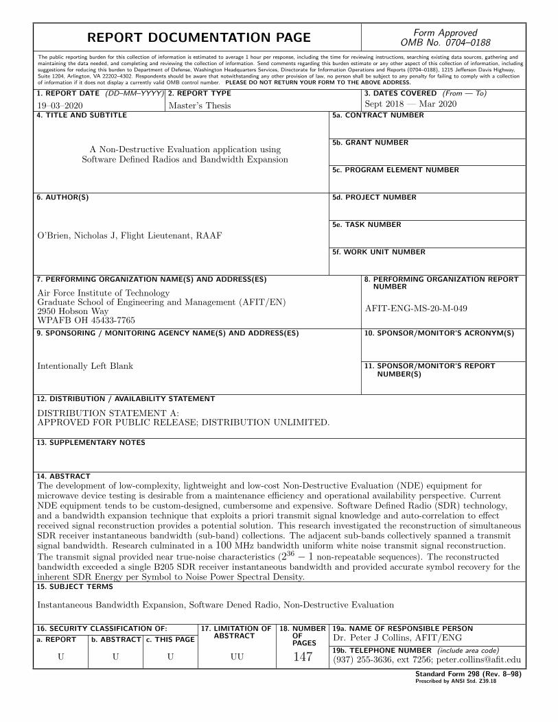
REPORT DOCUMENTATION PAGE Form ApprovedOMB No. 0704–0188
The public reporting burden for this collection of information is estimated to average 1 hour per response, including the time for reviewing instructions, searching existing data sources, gathering andmaintaining the data needed, and completing and reviewing the collection of information. Send comments regarding this burden estimate or any other aspect of this collection of information, includingsuggestions for reducing this burden to Department of Defense, Washington Headquarters Services, Directorate for Information Operations and Reports (0704–0188), 1215 Jefferson Davis Highway,Suite 1204, Arlington, VA 22202–4302. Respondents should be aware that notwithstanding any other provision of law, no person shall be subject to any penalty for failing to comply with a collectionof information if it does not display a currently valid OMB control number. PLEASE DO NOT RETURN YOUR FORM TO THE ABOVE ADDRESS.
1. REPORT DATE (DD–MM–YYYY) 2. REPORT TYPE 3. DATES COVERED (From — To)
4. TITLE AND SUBTITLE 5a. CONTRACT NUMBER
5b. GRANT NUMBER
5c. PROGRAM ELEMENT NUMBER
5d. PROJECT NUMBER
5e. TASK NUMBER
5f. WORK UNIT NUMBER
6. AUTHOR(S)
7. PERFORMING ORGANIZATION NAME(S) AND ADDRESS(ES) 8. PERFORMING ORGANIZATION REPORTNUMBER
9. SPONSORING / MONITORING AGENCY NAME(S) AND ADDRESS(ES) 10. SPONSOR/MONITOR’S ACRONYM(S)
11. SPONSOR/MONITOR’S REPORTNUMBER(S)
12. DISTRIBUTION / AVAILABILITY STATEMENT
13. SUPPLEMENTARY NOTES
14. ABSTRACT
15. SUBJECT TERMS
16. SECURITY CLASSIFICATION OF:
a. REPORT b. ABSTRACT c. THIS PAGE
17. LIMITATION OFABSTRACT
18. NUMBEROFPAGES
19a. NAME OF RESPONSIBLE PERSON
19b. TELEPHONE NUMBER (include area code)
Standard Form 298 (Rev. 8–98)Prescribed by ANSI Std. Z39.18
19–03–2020 Master’s Thesis Sept 2018 — Mar 2020
A Non-Destructive Evaluation application usingSoftware Defined Radios and Bandwidth Expansion
O’Brien, Nicholas J, Flight Lieutenant, RAAF
Air Force Institute of TechnologyGraduate School of Engineering and Management (AFIT/EN)2950 Hobson WayWPAFB OH 45433-7765
AFIT-ENG-MS-20-M-049
Intentionally Left Blank
DISTRIBUTION STATEMENT A:APPROVED FOR PUBLIC RELEASE; DISTRIBUTION UNLIMITED.
The development of low-complexity, lightweight and low-cost Non-Destructive Evaluation (NDE) equipment formicrowave device testing is desirable from a maintenance efficiency and operational availability perspective. CurrentNDE equipment tends to be custom-designed, cumbersome and expensive. Software Defined Radio (SDR) technology,and a bandwidth expansion technique that exploits a priori transmit signal knowledge and auto-correlation to effectreceived signal reconstruction provides a potential solution. This research investigated the reconstruction of simultaneousSDR receiver instantaneous bandwidth (sub-band) collections. The adjacent sub-bands collectively spanned a transmitsignal bandwidth. Research culminated in a 100 MHz bandwidth uniform white noise transmit signal reconstruction.The transmit signal provided near true-noise characteristics (236 − 1 non-repeatable sequences). The reconstructedbandwidth exceeded a single B205 SDR receiver instantaneous bandwidth and provided accurate symbol recovery for theinherent SDR Energy per Symbol to Noise Power Spectral Density.
Instantaneous Bandwidth Expansion, Software Dened Radio, Non-Destructive Evaluation
U U U UU 147
Dr. Peter J Collins, AFIT/ENG
(937) 255-3636, ext 7256; [email protected]