Ocean Modelling 85 (2015) 16–31

Contents lists available at ScienceDirect

Ocean Modelling

journal homepage: www.elsevier .com/locate /ocemod

A new vertical coordinate system for a 3D unstructured-grid model

http://dx.doi.org/10.1016/j.ocemod.2014.10.0031463-5003/� 2014 Elsevier Ltd. All rights reserved.

⇑ Corresponding author. Tel.: +1 (804) 684 7466; fax: +1 (804) 684 7179.E-mail address: yjzhang@vims.edu (Y.J. Zhang).

Yinglong J. Zhang a,⇑, Eli Ateljevich b, Hao-Cheng Yu d, Chin H. Wu c, Jason C.S. Yu d

a Virginia Institute of Marine Science, College of William & Mary, Center for Coastal Resource Management, 1375 Greate Road, Gloucester Point, VA 23062, USAb California Department of Water Resource, 1416 Ninth St Rm 215-4, Sacramento, CA 95814, USAc College of Engineering, Department Civil & Environmental Engineering, University of Wisconsin – Madison, 1415 Engineering Dr, Madison, WI 53706, USAd Dept. of Marine Environment and Engineering, National Sun Yat-Sen University, 70 Lien-Hai Road, Kaohsiung 80424, Taiwan

a r t i c l e i n f o

Article history:Received 1 April 2014Received in revised form 6 October 2014Accepted 30 October 2014Available online 15 November 2014

Keywords:LSC2

SELFEOcean and lake circulationUSAGreat LakesTaiwan

a b s t r a c t

We present a new vertical coordinate system for cross-scale applications. Dubbed LSC2 (Localized SigmaCoordinates with Shaved Cell), the new system allows each node of the grid to have its own vertical grid,while still maintaining reasonable smoothness across horizontal and vertical dimensions. Furthermore,the staircase created by the mismatch of vertical levels at adjacent nodes is eliminated with a simpleshaved-cell like approach using the concept of degenerate prisms. The new system is demonstrated tohave the benefits of both terrain-following and Z-coordinate systems, while minimizing their adverseeffects. We implement LSC2 in a 3D unstructured-grid model (SELFE) and demonstrate its superior per-formance with test cases on lake and ocean stratification.

� 2014 Elsevier Ltd. All rights reserved.

1. Introduction

The importance of the vertical coordinate system in ocean mod-eling has long been recognized. Three systems are commonly dis-cussed: (1) geo-potential coordinates (commonly referred to as‘Z’; Bryan, 1969; Cox, 1984); (2) terrain-following coordinates(sigma, S, c of Siddorn and Furner, 2013); and (3) isopycnal- orpressure-coordinates (Bleck and Chassignet, 1994). Each of thesecoordinate systems has advantages and disadvantages (Song andHou, 2006). For instance, Z and isopycnal coordinates are naturalto represent the neutral state of ocean stratification with nearlyhorizontal isopycnals, the numerical consequence of which is theadvantageous pre-cancellation of large components of pressurerepresenting that pressure balance. On the other hand, Z coordi-nates have issues with artificial staircases that hamper a good bot-tom representation and have been associated with artificial formdrag and discontinuous estimates of bed shear stress where thebed passes through layer interfaces. Several techniques have beenproposed to alleviate this problem (e.g., shaved cells); their imple-mentation is, however, often cumbersome.

Terrain-following coordinates better resolve the surface andbottom boundary layer and thus better represent topographicallydriven flow. However, a serious drawback of terrain-following

coordinates is that they lead to pressure gradient discretizationerrors (PGEs), which result in spurious flow near steep bottomslopes (Haney, 1991). Another issue related to diapycnal mixingstems from the fact that a coordinate plane generated from asloped bed transverses isopycnals, which in the transport stepresults in exaggerated transport between waters at differentdepths. The less commonly used isopycnal coordinates have theunique advantage of preserving mass for long-term simulation,but are problematic in well-mixed zones (Haidvogel andBeckmann, 1998). Hybridization of vertical coordinates has alsobeen successfully explored, e.g., by Zhang and Baptista (2008;hereafter ZB08) for SELFE, Barron et al. (2006) for NCOM, Bleckand Benjamin (1993) for HYCOM, in an effort to take advantageof the benefits from each system, but the implementation of thehybrid systems is non-trivial; a key factor is to ensure the smoothtransition between coordinates systems and avoid creating anumerical boundary layer.

In the real ocean, the horizontal and vertical dimensions are clo-sely coupled. However, the inter-play between horizontal and ver-tical grids is a subject that has not been carefully explored. Thereason may be that most ocean models use structured grids thatoffer little flexibility in the horizontal mesh. With little help com-ing from a judicious choice of horizontal grids, techniques focus onways to mitigate the issues associated with each vertical coordi-nate system. For example, a commonly used technique is tosmooth the bathymetry in order to reduce spurious flows resulting

Y.J. Zhang et al. / Ocean Modelling 85 (2015) 16–31 17

from terrain-following coordinates (Mellor et al., 1994). This dis-tortion of the problem geometry is unsatisfactory and affects tidalphase and other local and global properties of the flow field.Another example is the immersed boundary method which placesfictitious sources below bottom in order to satisfy the bottomboundary condition, a tactic which has implications for momen-tum (Mittal and Iaccarino, 2005). For problems associated withshear velocity and vertical profiles of turbulence, local remappingis used to solve vertical momentum diffusion on a more regularmesh (Platzek et al., 2012).

Some problems are further exacerbated as higher resolution isused in the models in order either to resolve small-scale processesor to include shallow-water regions. Indeed cross-scale river-estu-ary-shelf-ocean problems present significant challenges to models,many of which are exacerbated if the mesh does not adapt bothvertically and horizontally across scales. In the case of classic Zcoordinates, the global assignment of layer elevations precludeslocal adaptation at all. In terrain-following coordinates, wherethe number of layers is the same in deep and shallow regions, lay-ers crowd together in shallower water. Thin layers upstream exac-erbate the anisotropy already inherent in shallow water modelsand can make the roughness and turbulence closure discretizationsincongruent in different parts of the domain. Since parts of thedomain are resolved beyond ideal, there are also implications formodel performance. This is the case in our application to the Sac-ramento-San Joaquin Bay-Delta in California, where only a modestfraction of the domain near the Golden Gate and two ship channelsis markedly deep and steep.

Knowing we would face these tradeoffs, we deliberately choseto keep the vertical grid as flexible as possible when we weredeveloping an implicit unstructured-grid model (ZB08). The origi-nal SELFE model allows the use of two types of vertical coordinatesystems: terrain-following S coordinates (Song and Haidvogel,1994; hereafter SH94), and a partially S and partially Z (‘SZ’) systemwith the Z layers being placed beneath the S layers at a prescribeddemarcation depth (hs). The SZ system was implemented to allevi-ate PGEs, and has been shown to significantly improve the repre-sentation of the Columbia River plume (ZB08; Burla et al., 2010).However, as we will show later in this paper the transitionbetween S and Z layers can adversely attenuate momentum. Forthis reason, the demarcation depth often needs to be placed quitedeep, even though a shallower transition depth is better for controlof spurious mixing across isopycnals.

Alternate coordinates are easy to implement in our model. Asstated in the SELFE paper, the role of coordinates in SELFE is limitedto establishing the spacing and possible vertical time evolution ofthe mesh. Once the mesh is known, the underlying primitive equa-tions are solved untransformed in their original Cartesian form.Global coordinate systems such as Z and SZ are merely a conve-nient way to facilitate a layout with some advantageous propertiessuch as smooth transitions in time or space. However, given thediverse flow regimes in a typical domain, it is desirable to abandonthe rigid requirement of all nodes having equal number of levels(as in a terrain-following system) and allow each node to haveits own ‘localized’ grid based on geometry and problem-specificcriteria. The idea was originally proposed in Fortunato andBaptista (1996) in the context of simulating tidal flows, and theyoffered a few guidelines and an optimization procedure that can-not be applied to the more complex baroclinic problems consid-ered in this paper. More importantly, a significant challenge inLSC (Localized Sigma Coordinates) is caused by the staircase profilenear the bottom created because of a mismatch in the number oflevels along the horizontal domain. Similar approaches like hang-ing nodes have also been explored, but challenges remain in form-ing the required 3D control volumes for various equation solvers.

In this paper, we improve the vertical grid in SELFE by introduc-ing a new type of coordinate system called Localized Sigma Coor-dinates with Shaved Cell (LSC2), which belongs to the terrain-following class. We address the staircase issue with a novel andsimple shaved-cell-like approach. Unlike other shaved-cellapproaches which can be challenging to implement, our approachallows several bottom prisms to have degenerate heights. The ele-gance of this approach is that: (1) it completely eliminates thestaircase, leading to a smooth representation of the bottom whichis important for momentum; (2) the degenerate prism faces shutdown the exchange of tracer mass between deep and shallowregions, thus drastically reducing the diapycnal mixing, much asstaircases have done in the Z-coordinate models but without arti-ficial vertical ‘walls’ blocking the flow. The simplicity of the currentapproach and ease of implementation in a 3D model make it veryattractive as compared to other alternative approaches.

In Section 2, we briefly summarize the SELFE model and recentdevelopment. The new vertical grid system is then introduced inSection 3, and applied to two challenging test cases in Section 4:a lake stratification problem and the general circulation aroundTaiwan. The results are compared with observational data as wellas those from alternative vertical grids, to demonstrate the supe-rior performance of the new system. We conclude the paper withremarks on future work related to the optimal design of horizontaland vertical grids near steep slopes.

2. Description of SELFE

Introduced in 2008 (ZB08), SELFE is a 3D unstructured hydrody-namic model originally developed to address specific challengesfound in the Columbia River. It has since been used to modelnumerous other systems around the world (see the publication liston SELFE wiki [http://ccrm.vims.edu/w/index.php/Main_Page; lastaccessed in February 2014] for a complete list).

The model is grounded on a semi-implicit Finite ElementMethod with an Eulerian–Lagrangian Method (ELM) used to treatmomentum advection, and it has proved to be very effective inaddressing the challenges of cross-scale problems. The algorithmincorporates wetting and drying naturally and has been carefullybenchmarked for inundation (NTHMP, 2012; Zhang et al., 2011).As an open-source community-supported model, it has alsoevolved into a comprehensive modeling system that encompassesmany physical, chemical and biogeochemical processes (see refer-ences at the end of this section).

SELFE at its core solves the Reynolds-averaged Navier–Stokesequation in its hydrostatic form and transport of salt and heat:

Momentum equation:

DuDt¼ @

@zm@u@z

� �� grgþ F: ð1Þ

Continuity equation:

@g@tþr �

Z g

�hudz ¼ 0; ð2Þ

r � uþ @w@z¼ 0: ð3Þ

Transport equations:

@C@tþr � ðuCÞ þ @wC

@z¼ @

@zj@C@z

� �þ Fh þ Q ; ð4Þ

wherer @

@x ;@@y

� �.

(x,y) horizontal Cartesian coordinates.z vertical coordinate, positive upward.

18 Y.J. Zhang et al. / Ocean Modelling 85 (2015) 16–31

t time.g(x, y, t) free-surface elevation.h(x, y) bathymetric depth.u(x, y, z, t) horizontal velocity, with Cartesian components(u,v).w vertical velocity.F other forcing terms in momentum (baroclinicity, horizontalviscosity, Coriolis, earth tidal potential, atmospheric pressure,radiation stress).g acceleration of gravity, in [m s�2].C tracer concentration (e.g., salinity, temperature).m vertical eddy viscosity, in [m2 s�1].j vertical eddy diffusivity in [m2 s�1].Fh horizontal diffusion.Q mass source/sink.

The baroclinicity term is given by:

Fbc � �gq0

Z g

zrqd1

Eqs. (1)–(4) are completed by a turbulence closure (we use thegeneric length-scale model of Umlauf and Burchard (2003)), andproper initial and boundary conditions for each differentialequation.

In SELFE, ELM is used to integrate the advection operator in themomentum equation, then Eqs. (1) and (2) are solved simulta-neously for the unknown elevation defined at each node, with aGalerkin Finite Element Method. A semi-implicit time evolutionscheme is used so as to bypass the stringent CFL criterion (ZB08).The horizontal velocity is then solved from Eq. (1) with a Finite Ele-ment Method along each vertical direction at side centers of eachtriangular element. The vertical velocity is obtained from Eq. (3)as a diagnostic variable at element centroids using a Finite VolumeMethod for volume balance over prisms. Finally, the transportequations are solved with a Finite Volume Method (with anupwind or TVD scheme for advection) at prism centers. Note thatthe TVD scheme inside SELFE (Casulli and Zanolli, 2005) is explicitin time and 2nd-order in both horizontal and vertical dimension, asthe horizontal and vertical fluxes are coupled. Therefore the timestep used for the transport equation is usually one order of magni-tude smaller than that used for the momentum equation, and sub-cycling is required. To reduce the computational burden, users canset a threshold depth and specify a horizontal region where a moreefficient upwind scheme is used. An alternate, implicit TVD trans-port scheme is also soon to be introduced.

The combination of implicit treatment of gravity waves andpressure, ELM and unstructured grids has proved powerful inaddressing problems that traverse many spatial scales, as largetime steps can be used with high resolution. In fact, the time stepused in SELFE is constrained by an ‘inverse’ CFL criterion in order toavoid excessive truncation errors in the ELM (ZB08). Our experi-ence suggests CFL > 0.4 works well for most problems. On the otherhand, a very large CFL number will lead to a large truncation errorin the time discretization scheme. Therefore SELFE operates withinan operating range of time steps for a fixed grid, and convergence isguaranteed in the traditional sense when the time step and the gridsize approach zero at same rate (i.e. with the CFL number beingheld constant). An analogy to mode split models is that these mod-els also have an operating range for the grid size for a fixed timestep due to the condition CFL < 1, and convergence is also assuredwhen the time step and the grid size approach zero at same rate.

New model development of SELFE since 2008 includes:

(a) A new non-hydrostatic option based on the pressurecorrection method (Fringer et al., 2006).

(b) A spherical coordinate option based on Comblen et al.(2009).

(c) A new hydraulic structure module with application to Sacra-mento–San Joaquin Delta.

(d) Coupling to external models: Wind Wave Model (Rolandet al., 2012), oil spill model (Azevedo et al., 2014), EcoSim(Rodrigues et al., 2009), Community Sediment TransportModel (Pinto et al., 2012), and water quality model CE-QUAL-ICM (Wang et al., 2013).

3. Vertical discretization and coordinate system

SELFE is discretized with a 3D mesh that combines a general(but fixed) triangular unstructured mesh in the horizontal and astructured mesh in the vertical. The fundamental computationalunit is thus a triangular prism which in the non-degenerate casewill possess three faces normal to horizontal flow as well as atop and bottom face that can take on more arbitrary orientationas the free surface deforms under motion. The variables are thenstaggered along each prism.

The role of the vertical coordinate system in SELFE is to describethe vertical placement and evolution of nodes in the mesh. Oncethe mesh has been vertically remapped and the prism verticeslocated in Cartesian space for a particular time step, the dynamicequations (1)–(4) and supporting closures are solved in Z spacewithout transformation. Limiting the role of vertical coordinatesto the discretization is what gives SELFE its flexibility to swap innew coordinates.

The original SELFE implemented two types of vertical coordi-nate systems: terrain-following S coordinates (SH94; note thatthe sigma coordinates are a special case), and a hybrid system withZ layers placed near the bottom and S layers near the surface. TheSZ system was designed to alleviate the PGE near steep slopes(ZB08) but does introduce staircases in the Z zone (cf. Fig. 3(d)).One adverse consequence of the latter is the exaggeration of verti-cal velocity near those staircases due to artificial blocking of hori-zontal flow, as well as attenuation of horizontal momentum (cf.Fig. 10). Obviously these distortions have implications for tracertransport as well.

As far as cross-scale processes are concerned, an ideal verticalgrid should:

(a) resemble geo-potential coordinates in the interior of thewater column to minimize the slope of the coordinatesurface;

(b) follow the surface and bottom closely;(c) have a smooth transition in both the vertical and horizontal

direction; and(d) minimize computational cost.

A localized vertical grid can help satisfy all four requirementsabove. Perhaps the main challenge is related to (c), which isrequired to facilitate the calculation of gradients. In the originalLSC paper (Fortunato and Baptista, 1996) the authors proposed alocal coordinate system but ignored the horizontal transition issueas no horizontal gradients are calculated in their simplified tidalmodel. In this paper we use a particular type of LSC, the VanishingQuasi Sigma (VQS) proposed by Dukhovskoy et al. (2009). The VQSallows different number of vertical levels to be used at each hori-zontal location, determined by a series of reference grids definedat some pre-given depths, and thus effectively reduces the slopesof the sigma-coordinate surfaces. Dukhovskoy et al. (2009) pre-scribed three reference depths (from �1200 to �2000 m) in orderto resolve the slope of an escarpment in the Gulf of Mexico. Thebottom layer thickness was constrained by a minimum value(3 m in their paper) to avoid the thin layer syndrome found in Z-

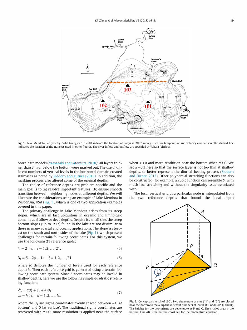
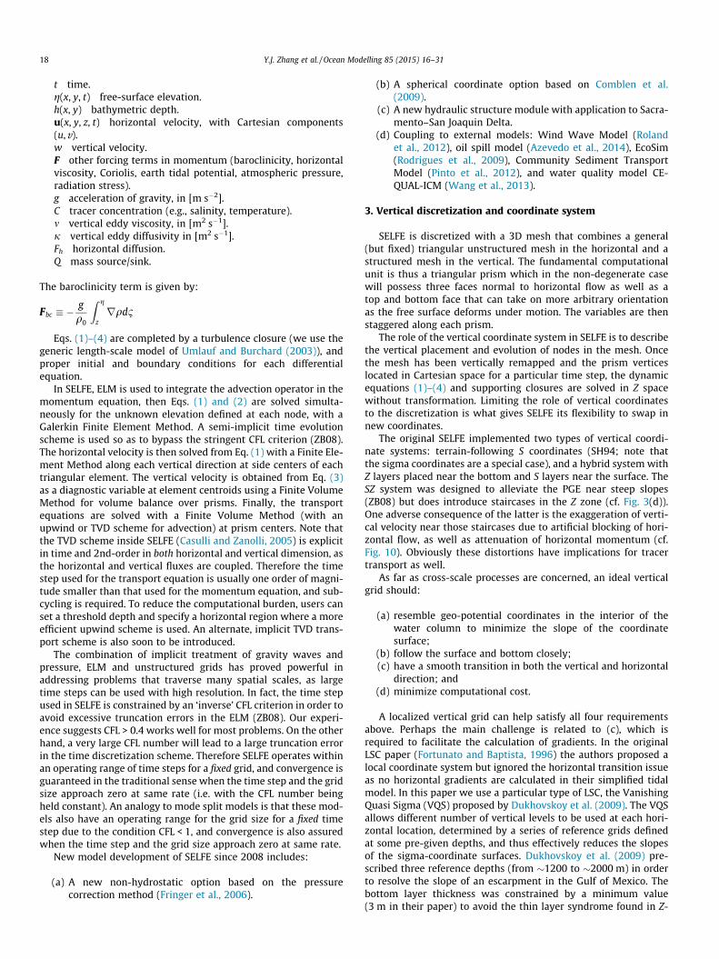
Fig. 1. Lake Mendota bathymetry. Solid triangles 101–103 indicate the location of buoys in 2007 survey, used for temperature and velocity comparison. The dashed lineindicates the location of the transect used in other figures. The river inflow and outflow are specified at Yahara (circles).

Fig. 2. Conceptual sketch of LSC2. Two degenerate prisms (‘‘1’’ and ‘‘2’’) are placednear the bottom to make up the different numbers of levels at 3 nodes (P, Q and R).The heights for the two prisms are degenerate at P and Q. The shaded area is thebottom. Line AB is the bottom-most cell for the momentum equation.

Y.J. Zhang et al. / Ocean Modelling 85 (2015) 16–31 19

coordinate models (Yamazaki and Satomura, 2010); all layers thin-ner than 3 m or below the bottom were masked out. The use of dif-ferent numbers of vertical levels in the horizontal domain createdstaircases as noted by Siddorn and Furner (2013). In addition, themasking process also altered some of the original depths.

The choice of reference depths are problem specific and themain goal is to (a) resolve important features; (b) ensure smoothtransition between neighboring nodes at different depths. We willillustrate the considerations using an example of Lake Mendota inWisconsin, USA (Fig. 1), which is one of two application examplescovered in this paper.

The primary challenge in Lake Mendota arises from its steepslopes, which are in fact ubiquitous in oceanic and limnologicdomains at shallow or deep depths. Despite its small size, the steepbottom slopes (up to 1:17) found in the lake are not dissimilar tothose in many coastal and oceanic applications. The slope is steep-est on the south and north sides of the lake (Fig. 1), which presentchallenges for terrain-following coordinates. For this system, weuse the following 21 reference grids:

hi ¼ 2þ i; i ¼ 1;2; . . . ;21; ð5Þ

Ni ¼ 6þ 2ði� 1Þ; i ¼ 1;2; . . . ;21; ð6Þ

where Ni denotes the number of levels used for each referencedepth hi. Then each reference grid is generated using a terrain-fol-lowing coordinate system. Since S coordinates may be invalid inshallow depths, here we use the following simple quadratic stretch-ing function:

r̂k ¼ ar2k þ ð1þ aÞrk;

zk ¼ hir̂k; k ¼ 1;2; . . . ;Ni;ð7Þ

where the rk are sigma coordinates evenly spaced between �1 (atbottom) and 0 (at surface). The traditional sigma coordinates arerecovered with a = 0; more resolution is applied near the surface

when a < 0 and more resolution near the bottom when a > 0. Weset a = 0.3 here so that the surface layer is not too thin at shallowdepths, to better represent the diurnal heating process (Siddornand Furner, 2013). Other polynomial stretching functions can alsobe constructed; for example, a cubic function can resemble S, withmuch less stretching and without the singularity issue associatedwith S.

The local vertical grid at a particular node is interpolated fromthe two reference depths that bound the local depth

Fig. 3. Comparison of vertical grids along the transect shown in Fig. 1, using (a) LSC2 (with maximum of 46 levels); (b) zoom-in view of the bottom showing severaldegenerate prisms; (c) 41 S levels, (d) 10S + 52Z, and (e) zoom-in view of (c).

20 Y.J. Zhang et al. / Ocean Modelling 85 (2015) 16–31

(Dukhovskoy et al., 2009). Unlike the original algorithm, we specifya minimum layer thickness of 0.2 m, but lump the last thin layerinto the layer above it so the local depth is not altered.

The staircases created by the mismatch of the number of levelsat adjacent nodes are eliminated with a shaved-cell approach viadegenerate prisms. Fig. 2 illustrates the concept of such anapproach. Wherever a mismatch exists, extra prisms are stackedbelow the smallest depth, and these prisms have at least 1 degen-erate height. The degenerate vertical faces of a prism (e.g., PQ inFig. 2) shut down the exchange of tracer mass without artificiallyblocking the flow (as in the case of a staircase); the bottom is faith-fully and smoothly represented in this way. Note that as far as the

momentum equation is concerned, the bottom-most face (AB inFig. 2) is not degenerate because the velocities are defined at sidecenters. Furthermore, the implementation of this new algorithminside SELFE is easy.

The combination of VSQ and degenerate prisms leads to thefinal LSC2 system. Fig. 3(a) shows the LSC2 grid along the verticaltransect across the lake as seen in Fig. 1. The zoomed-in view inFig. 3(b) shows several degenerate prisms near the bottom. For thissystem, a maximum of 46 levels is used to cover a depth of �23 m,and there are 73,620 active prisms. Much of the lake is consider-ably shallower than this depth and hence is associated with a smal-ler number of levels. Therefore, despite the seemingly large

Fig. 4. Temperature transect profile after 10 days for the diapycnal mixing test, for (a) S, (b) LSC2, (c) SZ grids, and (d) vertical profile at a location denoted by a star in (a). ‘i.c.’stands for initial condition. Note that a higher horizontal resolution is used in this plot than Fig. 3 in order to get a smooth visual. The differences between the profiles and theinitial condition are shown for (e) S, (f) LSC2, (g) SZ grids.

Y.J. Zhang et al. / Ocean Modelling 85 (2015) 16–31 21

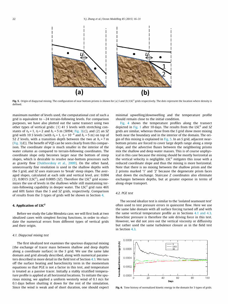
Fig. 5. Origin of diapycnal mixing. The configuration of near bottom prisms is shown for (a) S and (b) LSC2 grids respectively. The dots represent the location where density isdefined.

22 Y.J. Zhang et al. / Ocean Modelling 85 (2015) 16–31

maximum number of levels used, the computational cost of such agrid is equivalent to �24 terrain-following levels. For comparisonpurposes, we have also plotted out the same transect using twoother types of vertical grids: (1) 41 S levels with stretching con-stants of hb = 1, hf = 2 and hc = 5 m (SH94; Fig. 3(c)), and (2) an SZgrid with 10 S levels (with hb = 1, hf = 10�4 and hc = 5 m) on top of52 Z levels, with a transition depth between the two at hs = 7 m(Fig. 3(d)). The benefit of VQS can be seen clearly from this compar-ison. The coordinate slope is much smaller in the interior of thewater column as compared to terrain-following coordinates. Thecoordinate slope only becomes larger near the bottom of steepslopes, which is desirable to resolve near-bottom processes suchas gravity flow (Dukhovskoy et al., 2009). On the other hand,unnecessarily fine resolution is used in the shallow depths withthe S grid, and SZ uses staircases to ‘break’ steep slopes. The aver-aged slopes, calculated at each side and vertical level, are: 0.004(S), 0.0015 (LSC2), and 0.0005 (SZ). Therefore the LSC2 grid econo-mizes the use of levels in the shallows while still maintaining ter-rain-following capability in deeper water. The LSC2 grid runs 46%and 60% faster than the S and SZ grids, respectively. Comparisonof results from the 3 types of grids will be shown in Section 4.

4. Application of LSC2

Before we study the Lake Mendota case, we will first look at twoidealized cases with simplest forcing functions, in order to eluci-date the numerical errors from different types of vertical gridsand their origin.

Fig. 6. Time history of normalized kinetic energy in the domain for 3 types of grids.

4.1. Diapycnal mixing test

The first idealized test examines the spurious diapycnal mixing(the exchange of tracer mass between shallow and deep depthsalong a coordinate surface) in the S grid. We use the same lakedomain and grid already described, along with numerical parame-ters described in more detail in the field test of Section 4.3. We turnoff the surface heating and baroclinicity term in the momentumequations so that PGE is not a factor in this test, and temperatureis treated as a passive tracer. Initially a stably stratified tempera-ture profile is applied at all horizontal locations. To initiate the spu-rious mixing, we applied a uniform westerly wind of 0.1 m/s for0.1 days before shutting it down for the rest of the simulation.Since the wind is weak and of short duration, one should expect

minimal upwelling/downwelling and the temperature profileshould remain close to the initial condition.

Fig. 4 shows the temperature profiles along the transectdepicted in Fig. 1 after 10 days. The results from the LSC2 and SZgrids are similar, whereas those from the S grid show more mixingboth near the boundary and in the interior of the domain. The ori-gin of this mixing is explained in Fig. 5. In an S grid, adjacent near-bottom prisms are forced to cover large depth range along a steepslope, and the advective fluxes between the neighboring prismsmix the shallow and deep water masses. This is of course unphys-ical in this case because the mixing should be mostly horizontal asthe vertical velocity is negligible. LSC2 mitigates this issue with areduced coordinate slope and thus the mixing is more horizontal.Note that there is no mixing between the shallow prism and the2 prisms marked ‘1’ and ‘2’ because the degenerate prism facesshut down the exchange. Staircase Z coordinates also eliminateexchanges between depths, but at greater expense in terms ofalong-slope transport.

4.2. PGE test

The second idealize test is similar to the ‘isolated seamount test’often used to test pressure errors in quiescent flow. Here we usethe same lake domain with all surface forcing turned off and withthe same vertical temperature profile as in Sections 4.1 and 4.3.Baroclinic pressure is therefore the sole driving force in this test.However, we did not zero out the vertical viscosity or diffusivitybut rather used the same turbulence closure as in the field testin Section 4.3.

Fig. 7. Temperature transect profiles for the PGE test at the end of 100 days of simulation, with (a) S, (b) LSC2, and (c) SZ grid. Temperature profile at the starred location inFig. 4(a) is shown in (d).

Y.J. Zhang et al. / Ocean Modelling 85 (2015) 16–31 23

The analytical solution for this test is for the quiescent condi-tion and the initial stratification to persist. The main cause ofnumerical errors is the PGE coupled with turbulence mixingresulted from the spurious flow induced by PGEs.

We quantify the numerical error using normalized kineticenergy defined by:

NKE ¼

ffiffiffiffiffiffiffiffiffiffiffiffiffiffiffiffiffiffiffiffiffiffiffiffiffiffiffiffiffi0:5

Rqjuj2dV

0:5RqdV

s

where q is the fluid density and the integration is carried out overthe entire domain. Fig. 6 shows the time series of NKE for the 3types of grids. There is a sharp increase of NKE from the S grid ini-tially due to the initiation of motion by PGE, and a gradual decreaseafterward. The NKE from SZ and LSC2 are similar to each other anddo not exhibit the same sharp increase. At the end of a 100-day sim-ulation the NKEs from the 3 grids reach a quasi-steady state and arecomparable in magnitude (�0.4 mm/s). Although the spike in levelof NKE in the S grid is temporary, inspection of the final diffusedtemperature profile (Fig. 7) shows that the reduction comes at theexpense of work performed de-stratifying the water column. Spuri-ous flow and turbulent mixing in the S grid case have led to a morediffuse temperature profile than is evident in the results from theother 2 grids. As the temperature profile mixes, baroclinic forcingis weakened, which in turn reduces the spurious flow. In contrast,spurious flow caused by the SZ and LSC2 grids remains low through-out the simulation, with the thermal stratification remaining strong.

Fig. 8. NARR wind for the simulation period. Since the domain size is smallcompared to the NARR resolution, the wind is essentially uniform inside thedomain.

4.3. Field test of lake stratification

We now turn to tests of the same domain as in the earlier exam-ples, but under field conditions. Located near the Great Lakesregion of USA, Lake Mendota (43�400N, 89�240W) has a surface areaof 39.4 km2, shoreline length of 34 km, and a maximum fetch of9.8 km (Kamarainen et al., 2009). The deeper basin has a depth of

�23 m, which is sufficiently deep to maintain a stable thermalstratification during summer. Fig. 1 shows the bathymetry of LakeMendota.

Daily inflow measurements have been recorded on selectedtributaries of the lake since 1974, and daily outflow from the lakehas been measured since 1975. The measurements at Yahara Riverare used to drive the model; however, in the 2007 period studied inthis paper the flow rate is generally very small (<5 m3/s). Streamwater temperature has also been recorded at the Yahara River inletsince 2002, and the data can be downloaded from the website ofthe US Geological Survey (http://waterdata.usgs.gov/nwis; lastaccessed in February 2014).

Fig. 9. Comparison of temperature in 2007 at 3 buoy moorings between. (a) Observation; (b) SELFE with LSC2; (c) SELFE with SZ grid (with the transition depth at 7 m);(d) SELFE with 41 S levels, and (e) SELFE with SZ grid (with the transition depth at 14 m). Note that the time periods are different at the 3 buoys.

24 Y.J. Zhang et al. / Ocean Modelling 85 (2015) 16–31

In 2007, a field survey was conducted at Buoys 101–103 (Fig. 1),which were located at a water depths of 22.9 m, 19.8 m and22.9 m, respectively. HOBO Water Temperature Pros (with0.02 �C resolution, ±0.2 �C accuracy) were used to measure thewater temperature at a vertical interval of 2 m every 1 min. Watertemperature was measured from the end of May to the beginningof September at Buoy 101, from the end of July to mid-Septemberat Buoy 102 and from the end of July to the beginning of October atBuoy 103. The temperature profile data at the deeper Buoy 101provides the model with an initial condition, and the 3 differenttime periods cover the onset of stratification in late spring, the sta-bilization of the stratification in summer and its eventual destruc-tion in fall; therefore the data available allow validation of themodel on all three processes. In addition an acoustic Doppler Cur-rent Profiler (ADCP, RD Instruments) was placed at Buoy 103 to

acquire the current velocities of the water column with 1-m binsize, and the lowest bin was centered at 2.09 m above the lake bot-tom. The ping rate was 1 Hz and ensembles comprised 250 pingsevery five minutes.

Our unstructured grid of the lake consists of 1639 nodes and3064 triangles. The model runs start on June 8, 2007 with a timestep of 60 s. Besides the river forcing, the lake surface is also forcedby wind and heat fluxes taken from NCEP’s North AmericanRegional Reanalysis (NARR), with a 3-h temporal and �32 km spa-tial resolution. The coarse resolution of NARR certainly affects themodel results as discussed below, but do not affect the main find-ings. The wind is generally weak and does not show any preferentialdirection during the simulation period (Fig. 8). The bulk aerody-namic model of Zeng et al. (1998) is used to calculate the air-lakeexchange. The albedo is constant at 0.1, and the light attenuation

Fig. 10. Comparison of velocity at buoy 103 in 2007.

Y.J. Zhang et al. / Ocean Modelling 85 (2015) 16–31 25

depths for the water are taken from Jerlov type III water (Paulsonand Simpson, 1977). The turbulence closure of k–x as implementedby Umlauf and Burchard (2003) is used to calculate the turbulent

viscosity and diffusivities. The transport equations are solved withthe 2nd-order TVD scheme which introduces minimal numericaldiffusion in the horizontal and vertical directions.

Fig. 11. The ADCP record filtered with different cut-off periods.

26 Y.J. Zhang et al. / Ocean Modelling 85 (2015) 16–31

We conducted 4 simulations in order to compare the perfor-mance from three types of vertical grids available in SELFE (S, SZand LSC2), as described in Section 3 and illustrated in Fig. 3.Fig. 9(a)–(d) compares temperature results from the 3 verticalgrids with observations. The results from SZ and LSC2 are largelysimilar, and capture the initiation, stabilization and destructionof the thermal stratification from spring to fall. The timing of thesetransitions is also accurately simulated. On the other hand, theresults from the S grid show excessive mixing that quickly destroysthe stratification. Increasing the number of S levels to 62 onlyslightly delayed the destructive mixing (not shown). Furthermore,increasing the transition depth (hs) from 7 m to 14 m in the SZ grid,which makes it more like the S grid, also leads to more mixing(Fig. 9(e)). Therefore a small hs is required to obtain a reasonabletemperature profile when the SZ grid is used.

The surface temperature is slightly over-estimated by themodel. Analysis of long-term meteorological records indicates thatthe NARR has errors and biases in its estimates of air temperature(with a RMSE (Root-Mean-Square Error) of �2 �C) as well as wind(RMSE of �1 m/s). Therefore use of corrected air temperature andwind could further improve the results. Note that our main intentin this paper is to show that the modeled temperature at deeperdepths is accurate as it is less influenced by surface heating.

Although the SZ grid (with a proper choice of hs) captures thewater temperature quite well, its disadvantage becomes apparentwhen the velocity results are examined. Fig. 10 shows the velocity

comparison at Buoy 103 for about 21 days. The original ADCP con-tains strong signals from high-frequency internal waves (Fig. 11;see also Fig. 9(a)), which cannot be simulated with the hydrostaticmodel used here (Kamarainen et al., 2009). Therefore we applied aButterworth low-pass filter to the ADCP data with a cut-off periodof 4 h (Fig. 11 shows the unfiltered data as well as results fromother cut-off periods, and the results with 6-h cut-off are similarto those with 4-h cut-off). This time, the results from LSC2 gridsare closer to the S than to the SZ grid in terms of amplitudes; theresults from the SZ grid show large attenuation in the velocityamplitude due to the non-smoothness of the bottom representa-tion. This is confirmed by the calculated average amplitudes (viathe FFT function of Matlab): 4.84 (data), 3.37 (LSC2), 6.56 (S),0.73 (SZ with hs = 7 m), and 1.72 cm/s (SZ with hs = 14 m). Theseresults demonstrate that the new LSC2 grid has some of the advan-tages of the S and SZ grids while minimizing their shortcomings.

The velocity results from the LSC2 grid compare reasonably withthe ADCP data given the limitation of the hydrostatic assumption,and capture some episodic events (Fig. 10; see around August 20).The amplitude of the current is also reasonably simulated. Themodel does miss some events which may be attributed to thecoarse temporal resolution in NARR and/or the hydrostaticassumption. Since the non-hydrostatic signal is strong, a non-hydrostatic model is necessary to capture the full signal includingthe internal waves (Kamarainen et al., 2009). We are in the processof applying a new non-hydrostatic model to further explore this.

Fig. 12. (a) Marginal seas around Taiwan. The 8 stations where CTD casts were collected are indicated as red dots. (b) Unstructured grid. The horizontal bar indicates thelocation of the transect shown in Fig. 13.

Y.J. Zhang et al. / Ocean Modelling 85 (2015) 16–31 27

4.4. General circulation around Taiwan

The second example shows an oceanic application in the mar-ginal seas around Taiwan, where in places depths increase fromO(10 m) to >2000 m in �20 km, rendering a steep slope of 1:10or higher near continental shelf breaks (Fig. 12). Many complexbathymetric features are present in this region. The South ChinaSea (SCS) located to the south of this region is linked to the Pacificthrough the Luzon Strait between Taiwan and the Philippines, andto the East China Sea (ECS) through the Taiwan Strait (TWS). Thelatter is mostly shallow except for the Penghu Channel throughwhich most of inflow from the SCS takes place; the Channel and

the Chang-yun Rise to the north exert a major impact on the localflow pattern, and the volume transport there is correlated to theEast Asia Monsoon (Jan and Chao, 2003). The bathymetric slopeeast of Taiwan is generally very steep (cf. Fig. 12). The current sys-tem in this region is the subject of study by many authors usingobservations and numerical tools. A dominant process is the Kuro-shio which transports warm equatorial water northward from Phil-ippines island of Mindanao to Japan. Kuroshio often intrudes intothe SCS and ECS, and its extensions there interact with other cur-rent systems in a complex way (Liang et al., 2008; Oey et al.,2013). Other major coastal current systems include the TaiwanWarm Current that flows from the SCS to the ECS via the TWS,

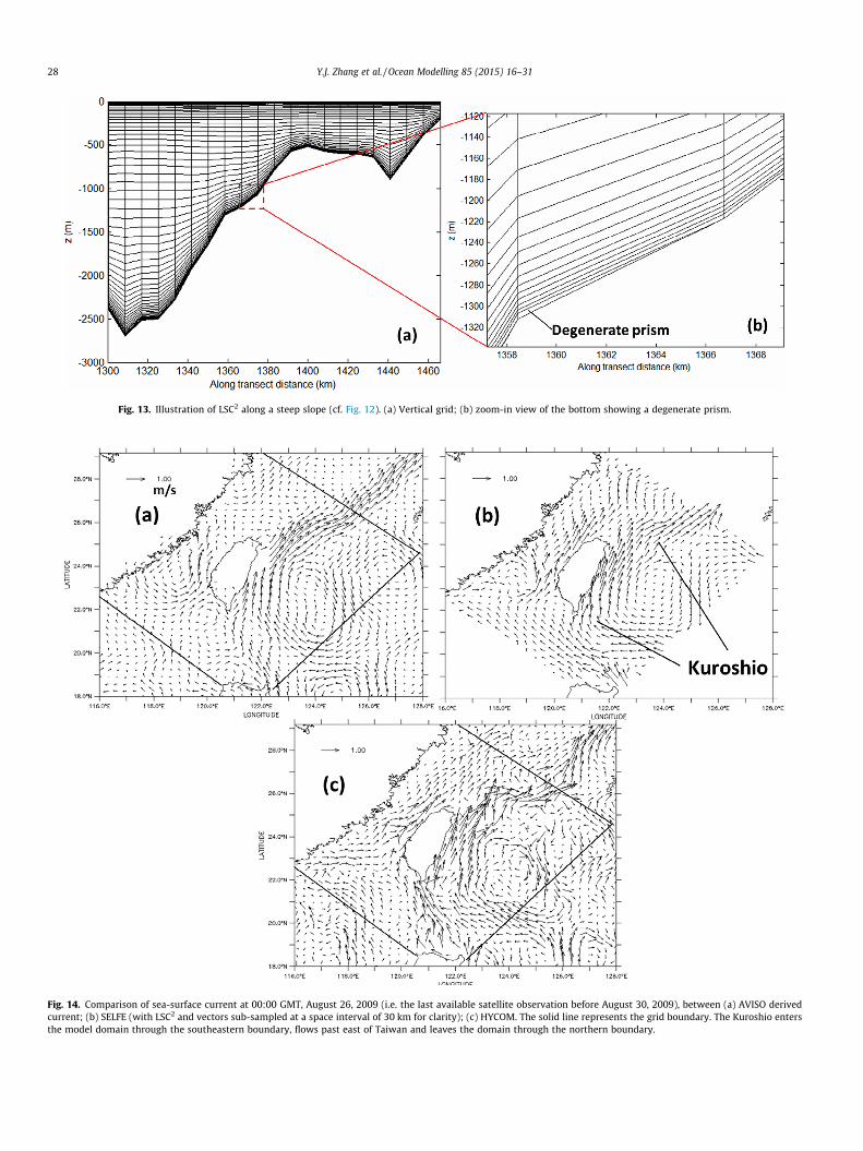
Fig. 13. Illustration of LSC2 along a steep slope (cf. Fig. 12). (a) Vertical grid; (b) zoom-in view of the bottom showing a degenerate prism.

Fig. 14. Comparison of sea-surface current at 00:00 GMT, August 26, 2009 (i.e. the last available satellite observation before August 30, 2009), between (a) AVISO derivedcurrent; (b) SELFE (with LSC2 and vectors sub-sampled at a space interval of 30 km for clarity); (c) HYCOM. The solid line represents the grid boundary. The Kuroshio entersthe model domain through the southeastern boundary, flows past east of Taiwan and leaves the domain through the northern boundary.

28 Y.J. Zhang et al. / Ocean Modelling 85 (2015) 16–31

Fig. 15. Comparison of SST at 00:00 GMT, August 30, 2009, between (a) GHRSST; (b) SELFE (with LSC2); (c) HYCOM.

Fig. 16. Comparison of temperature profiles at the 8 stations shown in Fig. 12(a), between CTD cast data, SZ grid and LSC2 grid. The first cast was taken shortly after the starttime of the simulation (June 1, 2009). The averaged RMSE’s are 1.49 �C (SZ) and 0.7 �C (LSC2).

Y.J. Zhang et al. / Ocean Modelling 85 (2015) 16–31 29

and the China coastal current that carries cold water southwardalong the Chinese coast. A multitude of eddies are found in thisregion, e.g., the cold dome frequently observed northeast of Taiwan(Shen et al., 2011). All these systems are forced by wind, heatfluxes and tides. The East Asia Monsoon in this region is dominatedby northeasterlies in winter and southwesterlies in summer, whichintroduce seasonal perturbations (Lee and Chao, 2003). Anomalousamplification of the M2 tide is observed in the middle of the TWSand is due to the wave reflection of the southward propagatingtidal wave by a deep trench in the southern strait (Jan et al.,2004), where a large amount of tidal energy is dissipated (Huet al., 2010).

Ours represents the first numerical study in this region using a3D unstructured-grid model. Our primary goal is to build a near-term operational model for the Central Weather Bureau of Taiwan.So far we have finished calibration of the model for different sea-sons in 2009, 2012 and 2013, although comprehensive reportingof our model skill assessment is beyond the scope of this paper.Here we focus on the improvement made possible by the introduc-tion of the new LSC2 grid, especially in the representation of thevertical stratification.

For this case, we use the following 39 reference grids:

hi ¼ 50þ 5iði� 1Þ; i ¼ 1;2; . . . ;39; ð8Þ

Ni ¼ 20þ i; i ¼ 1;2; . . . ;39: ð9Þ

Each reference grid is generated using S coordinates withstretching constants of hb = 1, hf = 5, and hc = 50 m, and a minimumbottom layer thickness of 3 m. Fig. 13 shows the LSC2 generatedalong a vertical transect with a steep slope east of Taiwan, andFig. 13(b) shows a degenerate prism near the bottom. A maximumof 94 levels is used to cover a maximum depth of �7200 m, andthere are 4,473,474 active prisms; the computational cost of sucha grid is equivalent to that of �24 terrain-following levels. Onceagain, the coordinate slope is much smaller in the interior of thewater column than with terrain-following coordinates, and thegrid is reasonably smooth in both the vertical and horizontaldirections.

For comparison purpose we have also used a SZ grid, with 26 Slevels placed on top of 8 Z levels with hs = 1000 m; the larger hs

value was chosen to avoid the attenuation issue discussed in the

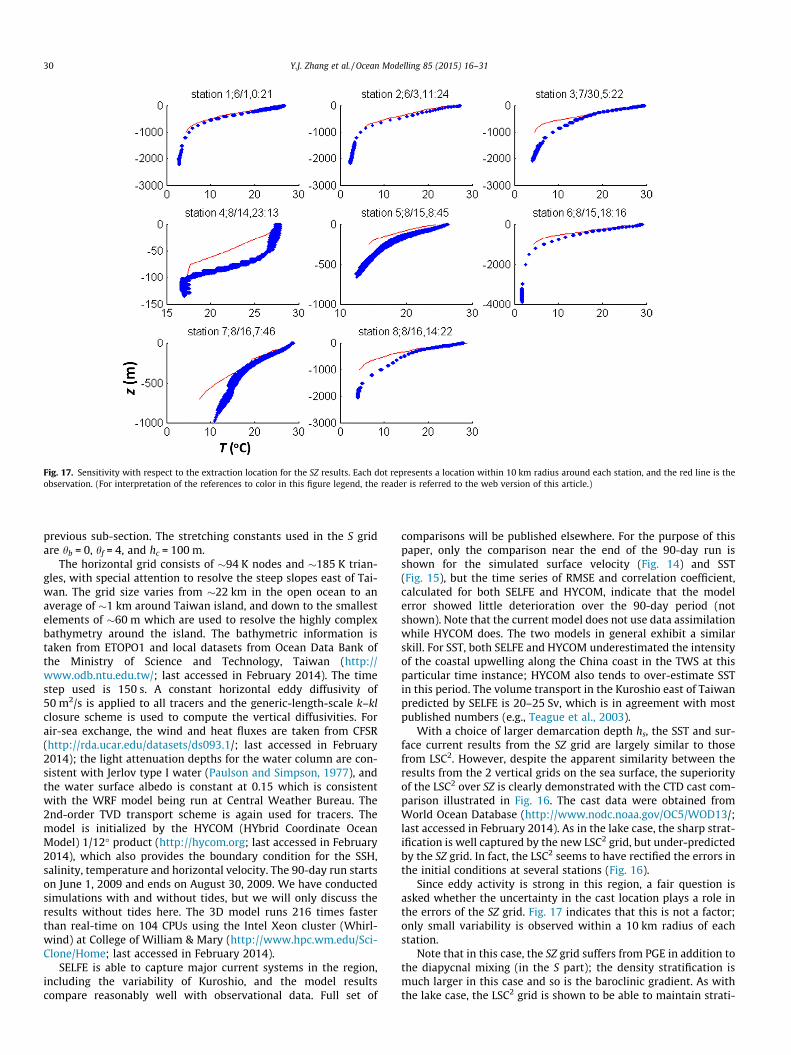
Fig. 17. Sensitivity with respect to the extraction location for the SZ results. Each dot represents a location within 10 km radius around each station, and the red line is theobservation. (For interpretation of the references to color in this figure legend, the reader is referred to the web version of this article.)

30 Y.J. Zhang et al. / Ocean Modelling 85 (2015) 16–31

previous sub-section. The stretching constants used in the S gridare hb = 0, hf = 4, and hc = 100 m.

The horizontal grid consists of �94 K nodes and �185 K trian-gles, with special attention to resolve the steep slopes east of Tai-wan. The grid size varies from �22 km in the open ocean to anaverage of �1 km around Taiwan island, and down to the smallestelements of �60 m which are used to resolve the highly complexbathymetry around the island. The bathymetric information istaken from ETOPO1 and local datasets from Ocean Data Bank ofthe Ministry of Science and Technology, Taiwan (http://www.odb.ntu.edu.tw/; last accessed in February 2014). The timestep used is 150 s. A constant horizontal eddy diffusivity of50 m2/s is applied to all tracers and the generic-length-scale k–klclosure scheme is used to compute the vertical diffusivities. Forair-sea exchange, the wind and heat fluxes are taken from CFSR(http://rda.ucar.edu/datasets/ds093.1/; last accessed in February2014); the light attenuation depths for the water column are con-sistent with Jerlov type I water (Paulson and Simpson, 1977), andthe water surface albedo is constant at 0.15 which is consistentwith the WRF model being run at Central Weather Bureau. The2nd-order TVD transport scheme is again used for tracers. Themodel is initialized by the HYCOM (HYbrid Coordinate OceanModel) 1/12� product (http://hycom.org; last accessed in February2014), which also provides the boundary condition for the SSH,salinity, temperature and horizontal velocity. The 90-day run startson June 1, 2009 and ends on August 30, 2009. We have conductedsimulations with and without tides, but we will only discuss theresults without tides here. The 3D model runs 216 times fasterthan real-time on 104 CPUs using the Intel Xeon cluster (Whirl-wind) at College of William & Mary (http://www.hpc.wm.edu/Sci-Clone/Home; last accessed in February 2014).

SELFE is able to capture major current systems in the region,including the variability of Kuroshio, and the model resultscompare reasonably well with observational data. Full set of

comparisons will be published elsewhere. For the purpose of thispaper, only the comparison near the end of the 90-day run isshown for the simulated surface velocity (Fig. 14) and SST(Fig. 15), but the time series of RMSE and correlation coefficient,calculated for both SELFE and HYCOM, indicate that the modelerror showed little deterioration over the 90-day period (notshown). Note that the current model does not use data assimilationwhile HYCOM does. The two models in general exhibit a similarskill. For SST, both SELFE and HYCOM underestimated the intensityof the coastal upwelling along the China coast in the TWS at thisparticular time instance; HYCOM also tends to over-estimate SSTin this period. The volume transport in the Kuroshio east of Taiwanpredicted by SELFE is 20–25 Sv, which is in agreement with mostpublished numbers (e.g., Teague et al., 2003).

With a choice of larger demarcation depth hs, the SST and sur-face current results from the SZ grid are largely similar to thosefrom LSC2. However, despite the apparent similarity between theresults from the 2 vertical grids on the sea surface, the superiorityof the LSC2 over SZ is clearly demonstrated with the CTD cast com-parison illustrated in Fig. 16. The cast data were obtained fromWorld Ocean Database (http://www.nodc.noaa.gov/OC5/WOD13/;last accessed in February 2014). As in the lake case, the sharp strat-ification is well captured by the new LSC2 grid, but under-predictedby the SZ grid. In fact, the LSC2 seems to have rectified the errors inthe initial conditions at several stations (Fig. 16).

Since eddy activity is strong in this region, a fair question isasked whether the uncertainty in the cast location plays a role inthe errors of the SZ grid. Fig. 17 indicates that this is not a factor;only small variability is observed within a 10 km radius of eachstation.

Note that in this case, the SZ grid suffers from PGE in addition tothe diapycnal mixing (in the S part); the density stratification ismuch larger in this case and so is the baroclinic gradient. As withthe lake case, the LSC2 grid is shown to be able to maintain strati-

Y.J. Zhang et al. / Ocean Modelling 85 (2015) 16–31 31

fication without adversely affecting the horizontal momentum,whereas the SZ grid is unable to accomplish both.

5. Concluding remarks

We have demonstrated the utility of a new type of vertical coor-dinate system, LSC2, based on the idea of Localized Sigma Coordi-nates (LSC, implemented in this paper using Vanishing QuasiSigma or VQS) and a simple shaved-cell technique using degener-ate near-bottom prisms. LSC2 has the benefits from the traditionalZ and terrain-following coordinates while minimizing their short-comings. Because the coordinate slope is much milder in LSC2 thanin the terrain-following coordinates, the resulting pressure gradi-ent errors are greatly reduced. LSC2 also has a smooth representa-tion of the bottom, and is completely free of staircases. The modelbetter represents bottom processes, as suggested by the results ofthis paper as well as those of many other test cases not shownhere. Finally, its implementation in a 3D model is relatively easyand avoids issues at the interface we encountered when combiningS and Z coordinate systems.

The new LSC2 can be best viewed as a generic framework whereother types of LSCs or even adaptive grids can be accommodated.Further research is needed for optimal design of horizontal andvertical grids near steep slopes, and to develop best practices forthe LSC2 grid in under-resolved regions. The latter may require alocally non-smooth vertical grid.

Acknowledgements

This research is sponsored by California Department of WaterResource (AECOM #60219187) and Central Weather Bureau of Tai-wan. Financial support for conducting field measurements in LakeMendota was provided by the National Science Foundation’s NorthTemperate Lakes LTER program. The authors would like to thankMs. Anastasia Gunawan for her help in some simulations and dataanalysis. Simulations shown in this paper were conducted on thefollowing HPC resources: (1) Sciclone at the College of Williamand Mary which were provided with the assistance of the NationalScience Foundation, the Virginia Port Authority, and Virginia’sCommonwealth Technology Research Fund; (2) the Extreme Sci-ence and Engineering Discovery Environment (XSEDE; Grant TG-OCE130032), which is supported by National Science FoundationGrant Number OCI-1053575; (3) NASA’s Pleiades.

References

Azevedo, A., Oliveira, A., Fortunato, A.B., Zhang, Y., Baptista, A.M., 2014. A cross-scalenumerical modeling system for management support of oil spill accidents. Mar.Pollut. Bull. 80, 132–147.

Barron, C.N., Kara, A.B., Martin, P.J., Rhodes, R.C., Smedstad, L.F., 2006. Formulation,implementation and examination of vertical coordinate choices in the globalnavy coastal ocean model (NCOM). Ocean Modell. 11, 347–375.

Bleck, R., Benjamin, S., 1993. Regional weather prediction with a model combiningterrain-following and isentropic coordinates. Part I: model description. Mon.Weather Rev. 121, 1770–1785.

Bleck, R., Chassignet, E.P., 1994. Simulating the oceanic circulation with isopycnic-coordinate models. In: Majumdar, S.K., Miller, E.W., Forbes, G.S., Schmalz, R.F.,Panah, A.A. (Eds.), The Oceans: Physical–Chemical Dynamics and HumanImpact. The Pennsylvania Academy of Science, pp. 17–39.

Bryan, K., 1969. A numerical method for the study of the circulation of the WorldOcean. J. Comput. Phys. 4, 347–376.

Burla, M., Baptista, A.M., Zhang, Y., Frolov, S., 2010. Seasonal and interannualvariability of the Columbia River plume: a perspective enabled by multiyearsimulation databases. J. Geophys. Res. 115, C00B16.

Casulli, V., Zanolli, P., 2005. High resolution methods for multidimensionaladvection–diffusion problems in free-surface hydrodynamics. Ocean Modell.10, 137–151.

Comblen, R., Legrand, S., Deleersnijder, E., Legat, V., 2009. A finite element methodfor solving the shallow water equations on the sphere. Ocean Modell. 28, 12–23.

Cox, M.D., 1984. A primitive equation three-dimensional model of the ocean. GFDLOcean Group Technical Report 1.

Dukhovskoy, D.S., Morey, S.L., O’Brien, J.J., Martin, P.J., Cooper, C., 2009. Applicationof a vanishing quasi-sigma vertical coordinate for simulation of high-speeddeep currents over the Sigsbee Escarpment in the Gulf of Mexico. Ocean Modell.28, 250–265.

Fortunato, A.B., Baptista, A.M., 1996. Vertical discretization in tidal flowsimulations. Int. J. Numer. Methods Fluids 22, 815–834.

Fringer, O.B., Gerritsen, M., Street, R.L., 2006. An unstructured-grid, finite-volume,nonhydrostatic, parallel coastal ocean simulator. Ocean Modell., 139–173.

Haidvogel, D.B., Beckmann, A., 1998. Numerical modeling of the coastal ocean. In:Brink, K.H., Robinson, A.R. (Eds.), The Sea, vol. 10, pp. 457–482.

Haney, R.L., 1991. On the pressure gradient force over steep topography in sigmacoordinate ocean models. J. Phys. Oceanogr. 21, 610–619.

Hu, C., Chiu, C., Chen, S., Kuo, J., Jan, S., Tseng, Y., 2010. Numerical simulation ofbarotropic tides around Taiwan. Terr. Atmos. Oceanic Sci. 21 (1), 71–84.

Jan, S., Chao, S., 2003. Seasonal variation of volume transport in the major inflowregion of the Taiwan Strait: the Penghu channel. Deep Sea Res. II 50, 1117–1126.

Jan, S., Chern, C., Wang, J., Chao, S., 2004. The anomalous amplification of M2 tide inthe Taiwan Strait. Geophys. Res. Lett. 31, L07308.

Kamarainen, A., Yuan, H.L., Wu, C.H., Carpenter, S.R., 2009. Estimates of phosphorusentrainment in Lake Mendota: a comparison of one-dimensional and three-dimensional approaches. Limnol. Oceanogr. Methods 7, 553–567.

Lee, H., Chao, S., 2003. A climatological description of circulation in and around theEast China Sea. Deep Sea Res. II 50, 1065–1084.

Liang, W., Yang, Y., Tang, T., Chuang, W., 2008. Kuroshio in the Luzon Strait. J.Geophys. Res. 113, C08048.

Mellor, G.L., Ezer, T., Oey, L.-Y., 1994. The pressure gradient conundrum of sigmacoordinate ocean models. J. Atmos. Oceanic Technol. 11, 1126–1134.

Mittal, R., Iaccarino, G., 2005. Immersed boundary methods. Annu. Rev. Fluid Mech.37, 239–261.

NTHMP, 2012. Proceedings and results of the 2011 NTHMP model benchmarkingworkshop. Boulder: US Department of Commerce/NOAA/NTHMP, NOAA SpecialReport 436p.

Oey, L., Chang, Y., Lin, Y., Chang, M., Xu, F., Lu, H., 2013. ATOP – the advanced Taiwanocean prediction system based on the mpiPOM. Part 1: model descriptions,analyses and results. Terr. Atmos. Oceanic Sci. 24 (1), 137–158.

Paulson, C.A., Simpson, J.J., 1977. Irradiance measurements in the upper ocean. J.Phys. Oceanogr. 7, 952–956.

Pinto, L., Fortunato, A.B., Zhang, Y., Oliveira, A., Sancho, F.E.P., 2012. Developmentand validation of a three-dimensional morphodynamic modelling system.Ocean Modell. 57–58, 1–14.

Platzek, F., Stelling, G., Jankowski, J., Patzwahl, R., 2012. On the representation ofbottom shear stress in z-layer models. In: Proceedings of HIC, 2012.

Rodrigues, M., Oliveira, A., Queiroga, H., Fortunato, A.B., Zhang, Y., 2009. Three-dimensional modeling of the lower trophic levels in the Ria de Aveiro(Portugal). Ecol. Model. 220 (9–10), 1274–1290.

Roland, A., Zhang, Y., Wang, H.V., Meng, Y., Teng, Y., Maderich, V., Brovchenko, I.,Dutour-Sikiric, M., Zanke, U., 2012. A fully coupled wave-current model onunstructured grids. J. Geophys. Res. Oceans 117, C00J33. http://dx.doi.org/10.1029/2012JC007952.

Shen, M., Tseng, Y., Jan, S., 2011. The formation and dynamics of the cold-dome offnortheastern Taiwan. J. Mar. Syst. 86, 10–27.

Siddorn, J.R., Furner, R., 2013. An analytical stretching function that combines thebest attributes of geopotential and terrain-following vertical coordinates. OceanModell. 66, 1–13.

Song, Y., Haidvogel, D., 1994. A semi-implicit ocean circulation model using ageneralized topography-following coordinate system. J. Comput. Phys. 115,228–244.

Song, Y.T., Hou, T.Y., 2006. Parametric vertical coordinate formulation formultiscale, Boussinesq, and non-Boussinesq ocean modeling. Ocean Modell.11, 298–332.

Teague, W.J., Jacobs, G.A., Ko, D.S., Tang, T.Y., Chang, K.-I., Suk, M.-S., 2003.Connectivity of the Taiwan, Cheju, and Korea Straits. Cont. Shelf Res. 23, 63–77.

Umlauf, L., Burchard, H., 2003. A generic length-scale equation for geophysicalturbulence models. J. Mar. Res. 6, 235–265.

Wang, H.V., Wang, Z., Loftis, J.D., Teng, Y.C., 2013. Hydrodynamic and water qualitymodeling and TMDL development for Maryland’s coastal Bays system, Finalreport submitted to Maryland Department of the Environment, TMDL TechnicalDevelopment Program.

Yamazaki, H., Satomura, T., 2010. Nonhydrostatic atmospheric modeling using acombined Cartesian grid. Mon. Weather Rev., 3932–3945.

Zeng, X., Zhao, M., Dickinson, R.E., 1998. Intercomparison of bulk aerodynamicalgorithms for the computation of sea surface fluxes using TOGA COARE andTAO data. J. Clim. 11, 2628–2644.

Zhang, Y., Baptista, A.M., 2008. SELFE: a semi-implicit Eulerian–Lagrangian finite-element model for cross-scale ocean circulation. Ocean Modell. 21 (3–4), 71–96.

Zhang, Y., Witter, R.C., Priest, G.R., 2011. Tsunami–tide interaction in 1964 PrinceWilliam sound tsunami. Ocean Modell. 40 (3–4), 246–259.