A new two-variable generalization of the chromatic polynomial
22
Discrete Mathematics and Theoretical Computer Science 6, 2003, 069–090 A new two-variable generalization of the chromatic polynomial Klaus Dohmen, Andr´ eP¨ onitz, Peter Tittmann Department of Mathematics, Mittweida University of Applied Sciences, 09648 Mittweida, Germany E-mail: [email protected], [email protected], [email protected] received July 31, 2002, revised February 20, 2003, May 15, 2003, June 12, 2003, accepted June 16, 2003. Let P(G; x, y) be the number of vertex colorings φ : V →{1, ..., x} of an undirected graph G =( V, E ) such that for all edges {u, v}∈ E the relations φ(u) ≤ y and φ(v) ≤ y imply φ(u) 6= φ(v). We show that P(G; x, y) is a polynomial in x and y which is closely related to Stanley’s chromatic symmetric function, and which simultaneously generalizes the chromatic polynomial, the independence polynomial, and the matching polynomial of G. We establish two general expressions for this new polynomial: one in terms of the broken circuit complex, and one in terms of the lattice of forbidden colorings. Finally, we give explicit expressions for the generalized chromatic polynomial of complete graphs, complete bipartite graphs, paths, and cycles, and show that P(G; x, y) can be evaluated in polynomial time for trees and graphs of restricted pathwidth. Keywords: chromatic polynomial, set partition, broken circuit, pathwidth, chromatic symmetric function 1 Introduction All graphs in this paper are assumed to be finite, undirected and without loops or multiple edges. We write G =( V, E ) to denote that G is a graph having vertex set V and edge set E . The well-known chromatic polynomial P(G; y) of a graph G =( V, E ) gives the number of vertex- colorings of G with at most y colors such that adjacent vertices receive different colors. For an introduction to chromatic polynomials the reader is referred to READ [7]. TUTTE [13, 14] has generalized the chromatic polynomial to the Tutte polynomial T (G; x, y). We propose a different generalization of the chromatic polynomial by weakening the requirements for proper colorings: Let X = Y ∪ Z, Y ∩ Z = / 0, be the set of available colors with |X | = x and |Y | = y. Then, a generalized proper coloring of G is a map φ : V → X such that for all {u, v}∈ E with φ(u) ∈ Y and φ(v) ∈ Y the relation φ(u) 6= φ(v) holds. Consequently, adjacent vertices can be colored alike only if the color is chosen from Z. In order to distinguish between these two sets of colors we call the colors of Y proper and the colors of Z improper. The number of generalized proper colorings of G is denoted by P(G; x, y), and as we will see in Theorem 1 below, this number turns out to be a polynomial in x and y, which we refer to as the generalized chromatic polynomial of G. Despite its simple definition, this new two-variable polynomial shows some interesting properties which are discussed later on in more detail: 1365–8050 c 2003 Discrete Mathematics and Theoretical Computer Science (DMTCS), Nancy, France
Transcript of A new two-variable generalization of the chromatic polynomial

Discrete Mathematics and Theoretical Computer Science6, 2003, 069–090
A new two-variable generalization of thechromatic polynomial
Klaus Dohmen, Andre Ponitz, Peter Tittmann
Department of Mathematics, Mittweida University of Applied Sciences, 09648 Mittweida, GermanyE-mail: [email protected], [email protected], [email protected]
received July 31, 2002, revised February 20, 2003, May 15, 2003, June 12, 2003, accepted June 16, 2003.
Let P(G;x,y) be the number of vertex coloringsφ : V→{1, ...,x} of an undirected graphG = (V,E) such that for alledges{u,v} ∈ E the relationsφ(u)≤ y andφ(v)≤ y imply φ(u) 6= φ(v). We show thatP(G;x,y) is a polynomial inxandy which is closely related to Stanley’s chromatic symmetric function, and which simultaneously generalizes thechromatic polynomial, the independence polynomial, and the matching polynomial ofG. We establish two generalexpressions for this new polynomial: one in terms of the broken circuit complex, and one in terms of the latticeof forbidden colorings. Finally, we give explicit expressions for the generalized chromatic polynomial of completegraphs, complete bipartite graphs, paths, and cycles, and show thatP(G;x,y) can be evaluated in polynomial time fortrees and graphs of restricted pathwidth.
Keywords: chromatic polynomial, set partition, broken circuit, pathwidth, chromatic symmetric function
1 IntroductionAll graphs in this paper are assumed to be finite, undirected and without loops or multiple edges. We writeG = (V,E) to denote thatG is a graph having vertex setV and edge setE.
The well-known chromatic polynomialP(G;y) of a graphG = (V,E) gives the number of vertex-colorings ofG with at mosty colors such that adjacent vertices receive different colors. For an introductionto chromatic polynomials the reader is referred to READ [7].
TUTTE [13, 14] has generalized the chromatic polynomial to the Tutte polynomialT(G;x,y). Wepropose a different generalization of the chromatic polynomial by weakening the requirements for propercolorings: LetX = Y ∪Z, Y ∩Z = /0, be the set of available colors with|X | = x and |Y | = y. Then,a generalized proper coloringof G is a mapφ : V → X such that for all{u,v} ∈ E with φ(u) ∈ Y andφ(v) ∈ Y the relationφ(u) 6= φ(v) holds. Consequently, adjacent vertices can be colored alike only if thecolor is chosen fromZ. In order to distinguish between these two sets of colors we call the colors ofYproper and the colors ofZ improper. The number of generalized proper colorings ofG is denoted byP(G;x,y), and as we will see in Theorem 1 below, this number turns out to be a polynomial inx andy,which we refer to as thegeneralized chromatic polynomialof G. Despite its simple definition, this newtwo-variable polynomial shows some interesting properties which are discussed later on in more detail:
1365–8050c© 2003 Discrete Mathematics and Theoretical Computer Science (DMTCS), Nancy, France

70 Klaus Dohmen, Andre Ponitz, Peter Tittmann
• It generalizes the chromatic polynomial, the independence polynomial, and the matching polyno-mial.
• It is closely related to Stanley’s chromatic symmetric function [11].
• It distinguishes all non-isomorphic trees with up to nine vertices.
• It satisfies both an edge decomposition formula and a vertex decomposition formula.
In subsequent sections, we give explicit expressions for the generalized chromatic polynomial of com-plete graphs, complete bipartite graphs, paths, and cycles, and show that our generalized chromatic poly-nomial can be evaluated in polynomial time for trees and graphs of restricted pathwidth.
2 Basic propertiesLet G = (V,E) be a graph, and letn = |V| andm = |E| denote the number of vertices and edges ofG,respectively. By consideringY = /0 we getP(G;x,0) = xn. The caseZ = /0 shows thatP(G;y,y) coincideswith the usual chromatic polynomialP(G;y). For any edgee∈E let G−eandG/ebe the graphs obtainedfrom G by deleting resp. contractingeand then, in the resulting multigraph, replacing each class of paralleledges by a single edge. By the edge decomposition formula for the usual chromatic polynomial we have
P(G;y,y) = P(G−e;y,y)−P(G/e;y,y). (1)
Since vertices belonging to different components ofG can be colored independently, we find that ifG1, ...,Gk are the connected components ofG, then
P(G;x,y) =k
∏i=1
P(Gi ;x,y) . (2)
The following theorem shows thatP(G;x,y) can be expressed in terms of chromatic polynomials ofsubgraphs ofG. Let G−X be the subgraph obtained fromG by removing all vertices of a vertex subsetX ⊆V. For short, we writeG−v instead ofG−{v}.
Theorem 1 Let G be a graph. Then,
P(G;x,y) = ∑X⊆V
(x−y)|X|P(G−X;y) .
Proof. Every generalized proper coloring ofG can be obtained by first choosing a subsetX of V thatis colored with colors ofZ. There are(x− y)|X| different colorings for these vertices. The remainingsubgraph has to be colored properly using colors ofY , for which there areP(G−X;y) possibilities. 2
Corollary 2 Let ai denote the number of independent vertex sets of cardinality n− i where n denotes thenumber of vertices of G. Then the independence polynomial of G, defined by I(G,x) := ∑n
i=0aixi , satisfies
I (G,x) = P(G;x+1,1) .
In particular, P(G;2,1) is the number of independent vertex sets of G.

A new two-variable generalization of the chromatic polynomial 71
Proof. By Theorem 1 we have
P(G;x+1,1) = ∑X⊆V
x|X|P(G−X;1) .
Note that the chromatic polynomialP(G−X;1) equals 1 ifV−X is an independent set (a set of isolatedvertices) ofG; otherwise,P(G−X;1) = 0. Consequently, the coefficient ofxi in P(G;x+1,1) counts theindependent sets of cardinalityn− i in G. 2
Theorem 3 The generalized chromatic polynomial P(G;x,y) satisfies
∂∂x
P(G;x,y) = ∑v∈V
P(G−v;x,y).
Proof. From Theorem 1 it follows that
∑v∈V
P(G−v;x,y) = ∑v∈V
∑W⊆V\{v}
(x−y)|W|P(G−W−v;y)
= ∑X⊆V|X|(x−y)|X|−1P(G−X;y)
=∂∂x
(∑
X⊆V(x−y)|X|P(G−X;y)
)
=∂∂x
P(G;x,y),
which gives the result. 2
We close this section by remarking that our generalized chromatic polynomial is not an evaluation ofthe Tutte polynomial [13,14]: The Tutte polynomialT(G;x,y) equalsxn−1 for every tree havingn verticesregardless of the structure of the tree. However, there are non-isomorphic trees with different generalizedchromatic polynomials. The smallest example for such a pair of trees is presented in Figure 1. Thegeneralized chromatic polynomials of these two treesP4 andS3 are respectively given by
P(P4;x,y) = x4−3x2y+y2 +2xy−y, (3)
P(S3;x,y) = x4−3x2y+3xy−y. (4)
Fig. 1: Non-isomorphic treesP4 andS3 having four vertices and distinct generalized chromatic polynomials.

72 Klaus Dohmen, Andre Ponitz, Peter Tittmann
3 The partition representation of P(G;x,y)Let G = (V,E) be a graph andΠ(V) be the partition lattice of the vertex setV. A subsetW ⊆ V isconnectedif the subgraph ofG induced by the vertices ofW is connected. LetΠG be the set of allpartitionsπ of V such that every block ofπ is connected. ThenΠG forms a geometric sublattice ofΠ(V)(see e.g. [10]). The unique minimal element0 in ΠG is the finest partition consisting only of singletons.We show thatΠG corresponds to thelattice of forbidden coloringsof G. Let f (π) be the number ofcolorings ofV with y proper colors andx−y improper colors such that
1. the vertices of each blockB of π all get the same color,
2. if |B|= 1 then that color can be any color ofX while if |B| ≥ 2 then that color must be fromY , and
3. no two blocks which are connected by an edge may be assigned the same color ofY .
Consequently, no proper coloring ofG contributes tof (π) for π > 0. We denote by|π| the number ofblocks ofπ. Let k1(π) be the number of singletons ofπ. We obtain
xk1(π)y|π|−k1(π) = ∑σ∈ΠGσ≥π
f (σ).
Our generalized chromatic polynomialP(G;x,y) corresponds tof (0). Thus, by Mobius inversion weobtain the following theorem.
Theorem 4 The generalized chromatic polynomial can be expressed as a sum over the latticeΠG:
P(G;x,y) = ∑π∈ΠG
µ(0,π)xk1(π)y|π|−k1(π). (5)
Fig. 2: A graph with four vertices
Consider the graphG shown in Figure 2. The latticeΠG of forbidden colorings ofG and the values ofthe Mobius functionµ(0,π) for this lattice is presented in Figure 3. The resulting polynomial is
P(G;x,y) = x4−4x2y+4xy+y2−2y.
In Eq. (5) the sum is extended over all blocksπ ∈ΠG. In the worst case this givesB(n) terms, whereB(n)denotes thenth Bell number. A combinatorial interpretation of the coefficients is given in the next section.

A new two-variable generalization of the chromatic polynomial 73
Fig. 3: Lattice of forbidden colorings for the graph in Figure 2.
STANLEY [11] defines thechromatic symmetric functionfor any graphG = (V,E) by
XG := ∑κ
∏i
x|κ−1(i)|
i
where the sum is over all proper coloringsκ : V → {1, . . . ,n} of G. Thus, the coefficient ofxλ11 · · ·xλr
r inXG is the number of proper colorings ofG such thatλk vertices are coloredk for k = 1, . . . , r. Stanleyshows that
XG = ∑π∈ΠG
µ(0,π)
pλ(π)
whereλ(π) denotes the type ofπ, that is,λ(π) = (λ1, . . . ,λr) where theλk’s denote the sizes of the blocksof π, and wherep denotes the power sum symmetric function, which forλ = (λ1, . . . ,λr) is defined by(cf. [11])
pλ :=|λ|
∏k=1
∑i
xλki ,
where |λ| denotes the number of parts ofλ. In view of this and Theorem 4, the coefficients of ourgeneralized chromatic polynomial and of Stanley’s chromatic symmetric function are related via the latticeΠG.
We proceed by establishing a connection between our polynomial and the matching polynomial. Recallthat amatchingof a graphG = (V,E) is a subsetF of E such that no two edges ofF share a commonvertex. Letmk be the number of matchings of cardinalityk in G. Thematching polynomialof G is definedby
M (G;x) :=bn/2c
∑k=0
(−1)k mkxn−2k.
Corollary 5 The matching polynomial is related to the generalized chromatic polynomial via[zn−2k
]M (G;z) =
[xn−2kyk
]P(G;x,y) ,
74 Klaus Dohmen, Andre Ponitz, Peter Tittmann
where[zn−2k
]M (G;z) and
[xn−2kyk
]P(G;x,y) denote the coefficients of zn−2k in M (G;z) and xn−2kyk in
P(G;x,y), respectively.
Proof. By Theorem 4 we have[xn−2kyk
]P(G;x,y) = ∑
π∈ΠGk1(π)=n−2k|π|=n−k
µ(0,π), (6)
where the Mobius function of an interval[0,π] in the partition lattice is given by (c.f. ROTA [8])
µ(0,π) = (−1)n−|π|∏A∈π
(|A|−1)! . (7)
HereA ∈ π indicates thatA is a block ofπ. A partition of {1, ...,n} with exactlyn−2k singletons andn−k blocks must contain exactlyk two-element blocks. Ifπ is such a partition, then Eq. (7) yields
µ(0,π) = (−1)k .
This is also the value of the Mobius function inΠG since the interval[0,π]
coincides with the correspond-ing interval of the partition lattice. Thus, Eq. (6) becomes[
xn−2kyk]
P(G;x,y) = (−1)k |{π ∈ΠG : k1(π) = n−2k, |π|= n−k}| .
Since there is a one-to-one correspondence between the set of partitions on the right-hand side of theformula and the set of matchings of cardinalityk, the statement of the corollary immediately follows.2
Thus the generalized chromatic polynomialP(G;x,y) incorporates the matching polynomial ofG aswell as the independence polynomial ofG. The matching polynomial and the independence polynomialare also related by the line graph via the identity (cf. [5])
M (G;x) = (−1)nxn−2mI(L(G) ;−x2) ,
but usingP(G;x,y) eliminates the need for usingL(G). Thus, our new polynomial may be considered as ageneralization of the chromatic polynomial, the independence polynomial, and the matching polynomial.
We proceed by establishing a representation of our new polynomial in terms of falling factorials. Apartitionπ of the vertex setV (G) is calledindependentif every block ofπ is an independent set ofG. Weuseλ ` n to denote thatλ is a number partition ofn. We obtain the following partition representation:
Theorem 6 For eachλ ` n= |V (G)|, let aλ be the number of independent partitions of G of typeλ. Then,the generalized chromatic polynomial satisfies
P(G;x,y) = ∑λ`n
aλy|λ|−k1(λ)k1(λ)
∑k=0
(k1 (λ)
k
)(x−y)k (y−|λ|+k1 (λ))k1(λ)−k ,
where yi denotes the falling factorial y(y−1) · · · (y− i +1).

A new two-variable generalization of the chromatic polynomial 75
Proof. The formula counts all proper generalized colorings ofG. To avoid multiple counting, wecolor all vertices of each block having more than one vertex by one proper color ofY . Different blockscontaining two or more vertices are colored differently. This givesy|λ|−k1(λ) possibilities to color theseblocks. The remaining singletons of the partition may be colored arbitrarily with proper colors or improperones. When using proper colors the singletons must be colored differently. This gives the second sum onthe right-hand side, and we are done. 2
Corollary 7 Let ai j be the number of independent partitions of G with exactly i singletons and j blockshaving two or more vertices. Then, the following equation holds:
P(G;x,y) =n
∑i=0
n
∑j=0
ai j
i
∑k=0
(ik
)(x−y)k yi+ j−k .
Corollary 7 suggests the introduction of a simpler two-variable polynomial of the form
Q(G;x,y) =n
∑i=0
n
∑j=0
ai j xiy j , (8)
which comprises the same amount of information as our generalized chromatic polynomial. However, thesimplicity of defining the polynomial in this way has to be paid for with loss of many nice properties, e.g.,the multiplicity with respect to components.
4 The coefficients in terms of broken circuitsOne of the most important results about the usual chromatic polynomial is Whitney’s broken circuit theo-rem [15], which expresses the coefficients of the chromatic polynomial in terms of broken circuits. Manyresults can be deduced directly from Whitney’s broken circuit theorem; see e.g., LAZEBNIK [6].
Let G = (V,E) be a graph where|V| = n andE is linearly ordered. Abroken circuitof G is obtainedfrom the edge set of a cycle ofG by removing its maximum edge. Thebroken circuit complexof G,abbreviated toBC (G), is the set of all non-empty subsets of the edge set not including any broken circuitas a subset. The definition of a broken circuit goes back to WHITNEY [15], while the broken circuitcomplex was initiated by WILF [16] and further investigated by BRYLAWSKI and OXLEY [2, 3]. In fact,BC (G) is an abstract simplicial complex in the sense of topology, whence we refer to eachI ∈ BC (G) asa faceof BC (G).
Whitney’s broken circuit theorem [15] states that for anyy∈ N,
P(G;y) =n
∑k=0
(−1)kbkyn−k ,
whereb0 = 1 andbk, k> 0, counts the faces of cardinalityk in the broken circuit complex ofG. Note thatwhile the definition of the broken circuit complex depends on the ordering of the edges, the same does notapply to thebk’s.
We now generalize Whitney’s broken circuit theorem to our new two-variable polynomialP(G;x,y).The proof of this generalization (and thus of Whitney’s original result) is facilitated by applying thefollowing inclusion-exclusion variant, which is an immediate consequence of [4, Corollary 3.5].

76 Klaus Dohmen, Andre Ponitz, Peter Tittmann
Proposition 8 Let {Ae}e∈E be a finite family of finite sets, where E is endowed with a linear orderingrelation. Furthermore, letF be a set of non-empty subsets of E such that for any F∈ F ,⋂
i∈F
Ai ⊆⋃
j>maxF
A j .
Then, ∣∣∣∣∣⋃e∈E
Ae
∣∣∣∣∣ = ∑I⊆E,I 6= /0
I 6⊇F(∀F∈F )
(−1)|I |−1
∣∣∣∣∣⋂i∈I
Ai
∣∣∣∣∣ .For any graphG = (V,E) and any subsetI of E we useG[I ] to denote the graph having vertex set{v∈V |v∈ e for somee∈ I} and edge setI .
We are now ready to state the main result of this section, which coincides withWhitney’s broken circuittheoremin the diagonal case wherex = y.
Theorem 9 Let G= (V,E) be a graph with n vertices and m edges and whose edge set is endowed witha linear ordering relation. Furthermore, let x∈ N and y∈ {0, . . . ,x}. Then,
P(G;x,y) =m
∑k=0
k
∑l=0
(−1)kbklxn−k−l yl , (9)
where b00 = 1 and bkl , k> 0, counts all faces I of cardinality k in the broken circuit complex of G suchthat G[I ] has exactly l connected components.
Proof. DefineF as the set of broken circuits ofG and for any edgeeof G define
Ae := { f : V→{1, . . . ,x}| f (u) = f (v)≤ y}, e= {u,v}.
Then, the requirements of Proposition 8 are satisfied, and thus we obtain
P(G;x,y) = xn−
∣∣∣∣∣⋃e∈E
Ae
∣∣∣∣∣ = xn +m
∑k=1
(−1)k ∑I∈BC (G)|I |=k
∣∣∣∣∣⋂i∈I
Ai
∣∣∣∣∣ . (10)
For any subsetI ∈BC (G) letmI , nI andcI denote the number of edges, vertices and connected componentsof the edge-subgraphG[I ], respectively. SinceG[I ] is cycle-free for anyI ∈ BC (G), we conclude thatmI −nI +cI = 0 and hence, ∣∣∣∣∣⋂
i∈I
Ai
∣∣∣∣∣ = xn−nI ycI = xn−mI−cI ycI . (11)
Now, put (11) into (10) and take into account thatcI ≤mI andmI = |I |. 2
In view of the results in [4] it can even be shown that for anyr ∈ N,
P(G;x,y)≤r
∑k=0
k
∑l=0
(−1)kbklxn−k−l yl (r odd),
P(G;x,y)≥r
∑k=0
k
∑l=0
(−1)kbklxn−k−l yl (r even),

A new two-variable generalization of the chromatic polynomial 77
wherebkl is defined as in Theorem 9. The proof of this ‘Bonferroni-like’ result is left to the reader.We further remark that the independence polynomialI(G;x) satisfies
I(G;x) =m
∑k=0
k
∑l=0
(−1)kbkl(x+1)n−k−l ,
which immediately follows fromI(G;x) = P(G;x+1,1) and Theorem 9, and that (9) can be restated as
P(G;x,y) = xnZ
(G;
1x,yx
),
where
Z(G;x,y) :=m
∑k=0
k
∑l=0
(−1)kbklxkyl .
Thus,ynZ(G;y−1,1) and(x+ 1)nZ(G;(x+ 1)−1,(x+ 1)−1) give the chromatic polynomial and the inde-pendence polynomial ofG, respectively.
As an example, consider the pathP4 and the starS3 in Figure 1. Letbkl andb′kl denote the coefficientsof P(P4;x,y) andP(S3;x,y), respectively. According to the interpretation of the coefficients provided byTheorem 9 we find that
b00 = 1, b22 = 1, b′00 = 1, b′22 = 0,
b10 = 0, b30 = 0, b′10 = 0, b′30 = 0,
b11 = 3, b31 = 1, b′11 = 3, b′31 = 1,
b20 = 0, b32 = 0, b′20 = 0, b′32 = 0,
b21 = 2, b33 = 0, b′21 = 3, b′33 = 0.
Putting these values into (9) we again obtain (3) and (4). The correspondingZ-polynomials are
Z(P4;x,y) = 1−3xy+2x2y+x2y2−x3y,
Z(S3;x,y) = 1−3xy+3x2y−x3y.
5 Special graphs5.1 The complete graph
The latticeΠG for the complete graphG = Kn coincides with the partition latticeΠ(V) of V, whereVdenotes the vertex set ofG. From (5) we obtain the equation
P(Kn;x,y) = ∑π∈Π(V)
µ(0,π)xk1(π)y|π|−k1(π), (12)
whereµ is the Mobius function of the partition lattice as defined in Eq. (7). A closer look at Eq. (12) revealsthat the terms of the sum do not depend on the partitionπ but only on its type. In the following, we use a

78 Klaus Dohmen, Andre Ponitz, Peter Tittmann
second representation for a number partitionλ. Besidesλ = (λ1, . . . ,λr) we also writeλ = (1k12k2...nkn)where eachki gives the number of parts of sizei in λ. Consequently,
n
∑i=1
ki = |λ| andn
∑i=1
iki = n,
and hence,
P(Kn;x,y) = n! ∑λ`n
(−1)n−|λ|
∏|λ|i=1 λi ∏ni=1ki !
xk1y|λ|−k1.
A simpler representation of this formula follows immediately from Corollary 7:
P(Kn;x,y) =n
∑k=0
(nk
)(x−y)kyn−k .
5.2 The complete bipartite graph
Let Km,n = (V ∪W,E) be the complete bipartite graph withm+ n = |V|+ |W| vertices. We choosekvertices fromV and color these vertices with proper colors. Let
{kj
}denote the Stirling number of the
second kind. Forj different colors there are{k
j
}y j different colorings. The remainingm− k vertices of
V may be colored with improper colors. No vertex ofW may receive one of thej proper colors that areused forV. Hence, we count(x− j)n different colorings for vertices ofW. Summing up all possibilities,we obtain
P(Km,n;x,y) =m
∑k=0
(mk
)(x−y)m−k
k
∑j=0
{kj
}y j(x− j)n .
As a special case, we obtain forSn = K1,n:
P(Sn;x,y) = xn(x−y)+y(x−1)n .
5.3 The path
Let Pn be the path withn vertices. As an example, we first consider the pathP5 as shown in Figure 4.
Fig. 4: The pathP5
The lattice of forbidden colorings forP5 is shown in Figure 5. We observe that this lattice is isomorphicto the Boolean latticeB4. More generally, the latticeΠPn is isomorphic to the Boolean latticeBn−1 (infact, ΠT is isomorphic toBn−1 for any treeT havingn vertices). The proof of this fact is rather easy. Aconnected partition of the vertex set of the pathPn with k blocks is generated by choosingk−1 separators

A new two-variable generalization of the chromatic polynomial 79
Fig. 5: The lattice of forbidden colorings forP5
between the elements of the linearly ordered set{v1, ...,vn}. A separator corresponds to a removed edgeof the path. In the following, we refer to such a partition as alinear partition. Now, by Theorem 4,
P(Pn;x,y) = ∑i, j
(−1)n−i− j l i j xiy j ,
wherel i j denotes the number of linear partitionsπ of v1,v2, . . . ,vn with i singletons blocks andj non-singleton blocks. All suchπ can be constructed as follows. Start with a diagram ofi + j−1 slashes whichcreatei + j spaces (between, before and after slashes) in which to place dots. Place one dot ini of thespaces and two dots in the remainingj. This can be done in
(i+ ji
)ways. Now distributen− i−2 j dots
among the spaces that already have two dots. The number of ways of doing this is the number of ways ofchoosingn− i−2 j objects fromj objects with repetition which equals(
j +(n− i−2 j)−1n− i−2 j
)=(
n− i− j−1n− i−2 j
).
Now replace then dots from left to right with the labelsv1,v2, . . . ,vn. The result is a linear partition withthe specified number of singleton and non-singleton blocks and every such partition is obtainable in thisway. Note that the total number of choices is
l i j =(
i + ji
)(n− i− j−1n− i−2 j
)as desired. Hence,
P(Pn;x,y) = ∑0<i+2 j≤n
(−1)n−i− j(
i + ji
)(n− i− j−1n− i−2 j
)xiy j .

80 Klaus Dohmen, Andre Ponitz, Peter Tittmann
For example, the polynomials of paths of up to five vertices are
P(P1;x,y) = x,
P(P2;x,y) = x2−y,
P(P3;x,y) = x3−2xy+y,
P(P4;x,y) = x4−3x2y+y2 +2xy−y,
P(P5;x,y) = x5−4x3y+3xy2 +3x2y−2y2−2xy+y .
Section 7 gives a method for obtaining the generalized chromatic polynomial of any tree by using apolynomial-time recursive algorithm.
5.4 The cycle
The last special graph to be considered here is the cycleCn. The construction of the lattice of forbiddencolorings differs only slightly from the construction of the corresponding lattice for the path. LetV ={v1, ...,vn} be the vertex set ofCn in correspondence with the order of traversing the cycle. A cyclicpartitionπ of V is one obtained by removing edges fromCn and using the resulting connected subsets ofvertices as blocks ofπ. Note that the lattice of cyclic partitions ofV is isomorphic toBn with the rank justbelow the maximum element removed. By Theorem 4,
P(Cn;x,y) = (n−1)(−1)n−1y+ ∑(i, j)6=(0,1)
(−1)n−i− jci j xiy j ,
whereci j denotes the number of cyclic partitions which havei singletons andj non-singletons. Thesecan be obtained as follows. As in Section 5.3, build a dot diagram which can be done inl i j ways wherel i j again denotes the number of linear partitions. Now turn the diagram into a cyclic partition by pickingone of then dots and then replacing the dots starting with that dot asv1, moving right, and then wrappingaround circularly to get the dots to the left ofv1. Thus we getnli j labeled diagrams. We claim that everycyclic partition is obtained exactlyi + j times. This is because any circular partition can be written withthe elementv1 in any of thei + j blocks. Sonli j = (i + j)ci j and hence,
ci j =n
i + j
(i + j
i
)(n− i− j−1n− i−2 j
).
Therefore,
P(Cn;x,y) = (−1)ny+n ∑0<i+2 j≤n
(−1)n−i− j
i + j
(i + j
i
)(n− i− j−1n− i−2 j
)xiy j .
For example, the generalized chromatic polynomial for cycles of up to five vertices are
P(C3;x,y) = x3−3xy+2y,
P(C4;x,y) = x4−4x2y+4xy+2y2−3y,
P(C5;x,y) = x5−5x3y+5xy2 +5x2y−5y2−5xy+4y.

A new two-variable generalization of the chromatic polynomial 81
6 Non-isomorphic graphs
Does the generalized chromatic polynomial distinguish non-isomorphic graphs? Two non-isomorphicgraphs having the same generalized chromatic polynomial must have the same chromatic polynomial,the same matching polynomial, and the same independence polynomial. Consequently, the number ofvertices, edges, and components must be the same for each such pair. The smallest non-isomorphic graphshaving the same generalized chromatic polynomial are depicted in Figure 6. We found by complete
Fig. 6: Non-isomorphic graphs having the same generalized chromatic polynomial.
enumeration that there is no pair of non-isomorphictreeswith up to nine vertices that have the samegeneralized chromatic polynomial. We found such a pair with 10 vertices which is presented in Figure 7.Note that the chromatic symmetric function, as defined by STANLEY [11], does not coincide for these two
Fig. 7: Non-isomorphic trees having the same generalized chromatic polynomial.
trees. The question whether the chromatic symmetric function distinguishes non-isomorphic trees is stillopen. We hope that our polynomial could be of some value to decide this question. The search for pairsof non-isomorphic trees having the same chromatic symmetric function can now be restricted to thosepairs of trees that have the same generalized chromatic polynomial. In this way (and using a computer)we found that there are no non-isomorphic trees with up to 15 vertices that have the same chromaticsymmetric function.

82 Klaus Dohmen, Andre Ponitz, Peter Tittmann
7 A polynomial algorithm for treesAs with the usual chromatic polynomial, the computation of the generalized chromatic polynomial is anNP-hard (in fact: #P-complete) counting problem. As a consequence, polynomial-time algorithms canonly be found for some restricted classes of graphs. In this section, we consider the restricted class oftrees.
Let P(G,W;x,y) be the generalized chromatic polynomial ofG with the additional restriction that thereis one proper color forbidden for all vertices of some given subsetW of V. Let C(G,v) be the set ofcomponents ofG− v. The following theorem provides an algorithm for computingP(G;x,y) for anytreeG.
Theorem 10 Let T be a tree and v∈V(T). Then, for each Ti ∈C(G,v) the set N(v)∩V(Ti) consists ofonly one vertex, and the polynomial P(T;x,y) can be computed via the following recursion:
P(T;x,y) = (x−y) ∏Ti∈C(T,v)
P(Ti ;x,y) + y ∏Ti∈C(T,v)
P(Ti ,N(v)∩V(Ti);x,y) ,
P(T,{v};x,y) = (x−y) ∏Ti∈C(T,v)
P(Ti ;x,y) + (y−1) ∏Ti∈C(T,v)
P(Ti ,N(v)∩V(Ti);x,y) .
If T only consists of v, then
P(T;x,y) = x,
P(T,{v};x,y) = x−1 .
Proof. Consider the first equation. Each vertex ofV can be colored with proper or improper colors.There are exactlyx− y possibilities to choose an improper color forv in which case the coloring ofthe neighbors ofv is independent of the color ofv. Consequently,v can be removed fromG. Thenumber of remaining colorings follows from the product formula (2). The second product of the firstequation arises from they different colorings ofv with proper colors. Now, the neighbors ofv have tobe colored differently fromv. The neighbor ofv in the subtreeTi is given byN(v)∩V(Ti). Indeed,this set contains exactly one vertex. The number of remaining colorings of the subtreeTi are given byP(Ti ,N(v)∩V(Ti);x,y). This shows the first formula. In order to prove the second formula we first remarkthat there are againx−y different colorings using only improper colors, which cause no restriction on thecomponents ofT− v. However, if we colorv with a proper color, then we have onlyy−1 possibilities.The remaining part is proved in a similar way. 2
Figure 8 illustrates the computation of the generalized chromatic polynomial for an example tree. Thedarkened vertices in this figure correspond to the vertices for which one color is forbidden. The decom-position vertex at each step is denoted byv. The resulting polynomial for the depicted tree is:
P(T;x,y) = (x−y)x3[(x−y)x2 +y(x−1)2
]+y(x−1)3[(x−y)x2 +(y−1)(x−1)2]
= x7−6x5y+9x4y+6x3y2−11x3y−9x2y2 +10x2y+5xy2−5xy−y2 +y.
There exists a vertexv in every tree withn vertices such that no component ofT − v has more thann/2 vertices. This vertex can be found in polynomial time as follows. Start with a randomly chosendecomposition vertexw. If T−w contains a componentTi with more then/2 vertices, then next choose

A new two-variable generalization of the chromatic polynomial 83
v
yx - y
x ( x - 1 )
y
y - 1x - yx - y
3 3
x 2( x - 1 ) 2
vv
Fig. 8: Computation of the generalized chromatic polynomial of a tree
the neighbor ofw belonging toTi . Repeating this procedure, we obtain after at mostn/2 steps a maximumcomponent with at mostn/2 vertices. By the appropriate combination of components, we can alwaysachieve a decomposition into three subtrees each consisting of at mostn/2 vertices.
Let f (n) be the time complexity of the recursive algorithm as described in Theorem 10 for the compu-tation of the generalized chromatic polynomial of any input tree of sizen = |V|. We find that
f (n)≤ 3 f(n
2
)+ p(n) , (13)
wherep(n) is a polynomial that incorporates the effort of the search for a decomposition vertex. For eachpolynomialp(n) inequality (13) leads to solutions which are polynomial inn. Consequently, we obtain apolynomial time algorithm for the computation of the generalized chromatic polynomial of a tree:
Corollary 11 The generalized chromatic polynomial of a tree can be computed in polynomial time.

84 Klaus Dohmen, Andre Ponitz, Peter Tittmann
Corollary 12 The generalized chromatic polynomial of a path Pn, n> 1, satisfies the recurrence relation
P(Pn;x,y) = (x−y)P(Pn−1;x,y)+y(y−1)n−2(x−1)+y(x−y)n−1
∑i=2
(y−1)i−2P(Pn−i ;x,y)
with the initial condition P(P1;x,y) = x.
Corollary 12 is an immediate consequence of Theorem 10.
8 Graphs of restricted pathwidthMany NP-hard graph problems become simple in graphs of restricted treewidth or pathwidth. A nice intro-duction to treewidth and related problems is given by BODLAENDER [1]. Here we present a polynomial-time algorithm for the computation of the generalized chromatic polynomial for graphs of restricted path-width. The main ideas may also be extended to cover graphs of restricted treewidth. The problem ofdetermining the pathwidth (treewidth) is NP-hard in general. If the pathwidth is known to be at mostkthen there is a polynomial-time algorithm for finding a path decomposition (composition order) of widthk.
A path decompositionof a graphG = (V,E) is a sequenceJ = (J0, ...,Jr) of subsets ofV such that
1.⋃r
i=0Ji = V, J0 = Jr = /0,
2. every edge ofG has both its vertices contained in at least one subset ofJ ,
3. for all i, j,k with 0≤ i < j < k≤ r the relationJi ∩Jk ⊆ Jj holds.
Thewidth of a path decompositionJ is the maximal cardinality of a subset ofJ . Thepathwidthof thegraphG is the minimum width over all path decompositions ofG. A path decompositionJ = (J0, ...,Jr)is callednice if |(Ji+1rJi)∪ (JirJi+1)|= 1 for all i = 0, ..., r−1. A nice path decompositionJ may bedescribed in terms of a sequenceS(J ) of signed verticesof G: The notation+v indicates the inclusion ofthe vertexv into the setJi while the notation−v stands for the removal ofv from Ji .
1
2
3
4
Fig. 9: Bridge graph.
For example, a nice path decomposition of the bridge graph presented in Figure 9 is
J = ( /0,{1},{1,2},{1,2,3},{2,3},{2,3,4},{3,4},{4}, /0) .
which is uniquely determined by the following sequence of signed vertices
S(J ) = (+1,+2,+3,−1,+4,−2,−3,−4) .

A new two-variable generalization of the chromatic polynomial 85
It follows from the definition of path decomposition that each vertex appears exactly once with positivesign and exactly once with negative sign inS(J ). Let J = (J0, ...,Jr) a path decomposition of widthk ofG. ThenJ can be transformed inO(n) time into a nice path decompositionJ of width at mostk (see [9]and [12]).
A composition orderof a graphG = (V,E) is a sequences= (s1, ...,st) of signed vertices and of edgesof G such that
1. if si ∈ s represents an edge with end verticesu andv then there are indicesj,k,m, p with j,k< i <m, p andsj = u, sk = v, sm =−u, sp =−v,
2. every edge ofG appears exactly once ins,
3. the removal of all edges froms yields a nice path decomposition ofG.
A composition order of the graph in Figure 9 is
s= (+1,+2,{1,2},+3,{1,3},−1,{2,3},+4,{2,4},−2,{3,4},−3,−4) . (14)
We refer to the objects in a composition order asstepsor, to be more precise, asvertex activation steps(positively signed vertices),vertex deactivation steps(negatively signed vertices), andedge insertionsteps. The composition order gives complete information about the graph structure, that is, no othergraph representation is required for the computation of the generalized chromatic polynomial.
Corollary 7 shows that the numbersapq of independent partitions consisting ofp singletons andq otherblocks give all the information which is necessary to determine the generalized chromatic polynomial ofG. The algorithm presented below computes these numbers directly. Some additional notation is needed.Let Gi be the graph consisting of all activated vertices and all edges inserted up to and including stepi ina composition orders, letVi be the vertex set ofGi , andAi be theset of active verticesof Gi , i.e.,Vi minusthe set of vertices deactivated up to and including stepi. A labeled partitionπ of Ai is a set partition ofAi
where blocks may have a label that will be denoted by a star (∗).For each independent partitionσ of Vi we define theinduced index ofσ as a tripleI = (π, p,q) consisting
of a labeled partitionπ of Ai and two integersp andq wherep equals the number of singletons ofσ andqis the number of blocks ofσ with more than one vertex. The blocks ofπ correspond to the restriction ofσto Ai , and a block ofπ is labeled iff the corresponding block ofσ is not a singleton. We note that differentpartitions ofVi may have the same induced index and refer to these partitions asrepresentedby the index.Let c be the number of partitions ofVi represented by the induced indexI . A pair (I ,c) will be called astateconsisting of theindex Iand thevalue c, and the set of all states at stepi defines thestate set Zi .
The main idea behind the algorithm is to compute the state setZi from the previous state setZi−1
according to certain rules depending on the stepsi of the given composition order.Obviously, the very first state setZ0 consists only of a single state(( /0,0,0),1), sinceV0 = /0 and since
there is only one partition of an empty set, and this partition contains neither singleton nor non-singletonblocks. More interestingly, the very last state setZr contains all the numbersapq. The set of active verticeswill be empty since each vertex has been activated and deactivated once. The partitions in the inducedindices are partitions of this active set and hence empty partitions. The valuesc corresponding to indicesI = (π, p,q) gives the numberapq of partitions of the full vertex set (sinceV2|V|+|E| = V) with p singletonandq non-singleton blocks.

86 Klaus Dohmen, Andre Ponitz, Peter Tittmann
The transformation rules for the state sets are as follows: For each stepsi , all states of the state setZi−1 are considered in turn leading to some (possibly empty) set ofintermediate successor states.Thesestates represent the same set of partitions as the original state but use the new active vertex set for theirdescription. After the individual states are transformed, there might be sets of such intermediate successorstates sharing the same index. These sets are replaced by single states using the common index and a valueequal to the sum of the values of states in the set. The states remaining after this clean-up form the nextstate setZi .
Vertex activation (+v): After activation stepsi activating some vertexv, this vertexv is a singleton inGi ,since no edge incident tov could have been introduced beforev became active. Sov is independentof all vertices inGi−1 and hence, it can extend any independent set ofGi−1. Suppose we needto transform a statez = (I ,c) with I = (π, p,q). Let S= {σ1,σ2, . . .} be the set of independentpartitions consisting ofp singletons andq non-singleton blocks that induceI . We then proceed asfollows:
• First of all, note that the new vertexv can form a singleton block of its own in any of theσk.In this case, the number of singletons increases by one, andv forms a new unlabeled blockof π. Everything else remains unchanged, leading to a single intermediate successor state of((π|v, p+1,q),c), whereπ|v is the partition obtained by augmentingπ by a single block{v}.
• Secondly, sincev is independent of all vertices inGi−1, it is certainly independent of thevertices that constitute any of theq non-singleton blocks of someσk. Hence,v can be addedto any such block, which results in a block of cardinality larger than one. LetX be such anon-singleton block and defineY := X∩Ai−1. We have to distinguish two cases: (a) IfY = /0,then v will be a singleton in(X + {v})∩Ai . Since|X ∪ {v}| > 1 it must be marked, andthus the single successor state is((π|v∗, p,q),c). (b) If Y 6= /0, then we already have partsof X in the active vertex set, namely the vertices ofY. In this case, the successor state is((π−Y|(Y∪{v})∗ , p,q),c).
• Similarly to the above, the new vertexv can be added to allp singleton blocks. This works ina similar way with one exception: the singleton grows to a non-singleton block, whence wehave to decrementp and incrementq by one in the successor state.
Vertex deactivation (−v): If I = (π, p,q) describes a set of independent partitions ofGi−1, then(π−v, p,q) describes the same set forGi whereπ− v is π−{v} in case thatv is a singleton resp.π−X|Xr {v} in case thatv∈ X for a larger blockX of π. So for deactivation, every state has asingle intermediate successor state, which is obtained by removing the vertex for the partition in theindex partition.
Edge insertion {u,v}: Let I , w andπ be defined as in the vertex activation step above. Ifπ is a partitioncontaining a blockX with {u,v} ⊆ X then this block forms no independent set inGi asGi resultsfrom Gi−1 by inserting edge{u,v}. Consequently, the state(I ,c) has no successor states as thereare no independent partitions inducingπ in Gi .
As an example, we compute the generalized chromatic polynomial of the bridge graph depicted inFigure 9. The resulting transformations using the composition order given by (14) are presented in Table
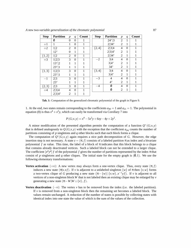
A new two-variable generalization of the chromatic polynomial 87
Step Partition p q Count/0 0 0 1
+1 1 1 0 1+2 1|2 2 0 1
12∗ 0 1 1{1,2} 1|2 2 0 1+3 1|2|3 3 0 1
13∗|2 1 1 123∗|1 1 1 1
{1,3} 1|2|3 3 0 123∗|1 1 1 1
−1 2|3 3 0 123∗ 1 1 1
{2,3} 2|3 3 0 1+4 2|3|4 4 0 1
2|3|4∗ 2 1 1
Step Partition p q Count24∗|3 2 1 12|34∗ 2 1 1
{2,4} 2|3|4 4 0 12|3|4∗ 2 1 12|34∗ 2 1 1
−2 3|4 4 0 13|4∗ 2 1 134∗ 2 1 1
{3,4} 3|4 4 0 13|4∗ 2 1 1
−3 4 4 0 14∗ 2 1 1
−4 /0 4 0 1/0 2 1 1
Tab. 1: Computation of the generalized chromatic polynomial of the graph in Figure 9.
1. At the end, two states remain corresponding to the coefficientsa40 = 1 anda21 = 1. The polynomial inequation (8) is thusx4 +x2y, which can easily be transformed via Corollary 7 into
P(G;x,y) = x4−5x2y+6xy−4y+2y2.
A minor modification of the presented algorithm permits the computation of a functionQ∗ (G;x,y)that is defined analogously toQ(G;x,y) with the exception that the coefficientapq counts the number ofpartitions consisting ofp singletons andq other blocks such that each block forms a clique.
The computation ofQ∗(G;x,y) again requires a nice path decomposition ofG. However, the edgeinsertion step is not necessary. A statez= (π, f ) consists of a labeled partitionπ as index and a bivariatepolynomial f as value. This time, the label of a block ofπ indicates that this block belongs to a cliquethat contains already deactivated vertices. Such a labeled block can not be extended to a larger clique.The coefficient[xpyq] f of the polynomialf gives the number of partitions represented by the indexπ thatconsist ofp singletons andq other cliques. The initial state for the empty graph is( /0,1). We use thefollowing elementary transformations:
Vertex activation (+v): A new vertex may always form a one-vertex clique. Thus, every state(π, f )induces a new state(π|v,x f). If v is adjacent to a unlabeled singleton{w} of π then{v,w} formsa two-vertex clique ofG producing a new state
(π−{w}|{v,w} ,x−1y f
). If v is adjacent to all
vertices of a non-singleton blockW that is not labeled then an existing clique may be enlarged byvgenerating a new state(π−W|W∪{v} , f ).
Vertex deactivation (−v): The vertexv has to be removed from the index (i.e. the labeled partition).If v is removed from a non-singleton block then the remaining set becomes a labeled block. Thevalues remain unchanged. A reduction of the number of states is possible by collecting states withidentical index into one state the value of which is the sum of the values of the collection.

88 Klaus Dohmen, Andre Ponitz, Peter Tittmann
The application of this algorithm to the graph of Figure 9 yields
Q∗(G;x,y) = y4 +5xy2 +2xy+2x2.
Let G be the complement of the graphG. It follows from the definition ofQ∗ that Q(G;x,y) =Q∗(G;x,y
). This gives the following result:
Theorem 13 The generalized chromatic polynomial can be computed in polynomial time for graphs of re-stricted pathwidth and for graphs whose complement is of restricted pathwidth. In particular, the matchingpolynomial, the independence polynomial, and the chromatic polynomial can be computed in polynomialtime for graphs of restricted pathwidth and for graphs whose complement is of restricted pathwidth.
AcknowledgementThe authors wish to express their gratitude to the referees for the many helpful suggestions that resultedin an improvement of the paper. In particular, the derivations of the generalized chromatic polynomial ofa path (Subsection 5.3) and a cycle (Subsection 5.4) were greatly simplified by one of the referees, whosesolution we adopted with minor changes and whom we especially would like to thank for his worthycontribution.
References[1] H.L. Bodlaender: A partialk-arboretum of graphs with bounded treewidth,Theoret. Comput. Sci.
209(1998), 1–45.
[2] T. Brylawski: The broken circuit complex,Trans. Amer. Math. Soc.234(1977), 417–433.
[3] T. Brylawski & J. Oxley: The broken-circuit-complex: its structure and factorizations,Europ. J.Comb.2 (1981), 107–121.
[4] K. Dohmen: Improved Bonferroni inequalities via union-closed set systems,J. Combin. Theory Ser.A 92 (2000), 61–67.
[5] C. Godsil & G. Royle: Algebraic Graph Theory, Graduate Texts in Mathematics, 207, Springer-Verlag, New York, 2001.
[6] F. Lazebnik: Some corollaries of a theorem of Whitney on the chromatic polynomial,Discrete Math.87 (1991), 53–64.
[7] R.C. Read: An introduction to chromatic polynomials,J. Combin. Theory Ser. B4 (1968), 52–71.
[8] G.-C. Rota: On the Foundations of Combinatorial Theory: I. Theory of Mobius functions,Z.Wahrscheinlichkeitstheorie Verw. Gebiete2 (1964), 340–368.
[9] P. Scheffler: Die Baumweite von Graphen als ein Maß fur die Kompliziertheit algorithmischerProbleme, Report R-MATH-04/89, Karl-Weierstraß-Institut fur Mathematik, Akademie der Wis-senschaften der DDR, Berlin, 1989.
[10] R.P. Stanley:Enumerative Combinatorics, Vol. 1, Wadsworth & Brooks/Cole, Monterey, Ca., 1986.

A new two-variable generalization of the chromatic polynomial 89
[11] R.P. Stanley:Enumerative Combinatorics, Vol. 2, Cambridge University Press, 1999.
[12] D.M. Thilikos, M.J. Serna, H.L. Bodlaender: Constructive linear time algorithms for small cutwidthand carving-width, Proc. 11th International Symposium on Algorithms and Computation, ISAAC’00, Lecture Notes in Computer Science 1969, Springer Verlag, 2000, pp. 192–203.
[13] W.T. Tutte:Graph Theory, Addison-Wesley, Menlo Park, 1984.
[14] W.T. Tutte: A ring in graph theory,Proc. Cambridge Phil. Soc.43 (1947), 26–40.
[15] H. Whitney: A logical expansion in mathematics,Bull. Amer. Math. Soc.38 (1932), 572–579.
[16] H.S. Wilf: Which polynomials are chromatic?,Proc. Colloquio Internazionale sulle Teorie Combi-natorie (Roma, 1973), Tomo I, Atti dei Convegni Lincei, No. 17, Accademia Naz. Lincei (Rome),1976, pp. 247–256.

90 Klaus Dohmen, Andre Ponitz, Peter Tittmann