Coastal Engineering, 2 (1978) 21--39 21 © Elsevier Scientific Publishing Company, Amsterdam -- Printed in The Netherlands

A NEW PHOTOGRAMMETRIC METHOD FOR DETERMINING SHORELINE EROSION

ROBERT DOLAN, BRUCE HAYDEN and JEFFREY HEYWOOD

Department of Environmental Sciences, University of Virginia, Charlottesville, Va. (U.S.A.)

(Received July 11, 1977; accepted December 1, 1977)

ABSTRACT

Dolan, R., Hayden, B. and Heywood, J., 1978. A new photogrammetric method for determining shoreline erosion. Coastal Eng., 2: 21--39.

In order to systematically measure shoreline erosion and storm surge penetration along extensive reaches of the United States Atlantic coast, a common-scale mapping method was developed using historical aerial photography as the data base. Aerial photography of the southern New Jersey coast covering four decades is used to demonstrate the method- ology and to provide long-term baseline information on shoreline dynamics. The data sets include mean erosion rates and variance at 100-m intervals along the coast. Shoreline recession rates along the New Jersey coast are generally less than 1 m/yr. but for several locations rates exceed 5 m/yr., and they vary considerably both within and between the island segments of the New Jersey coast.

INTRODUCTION

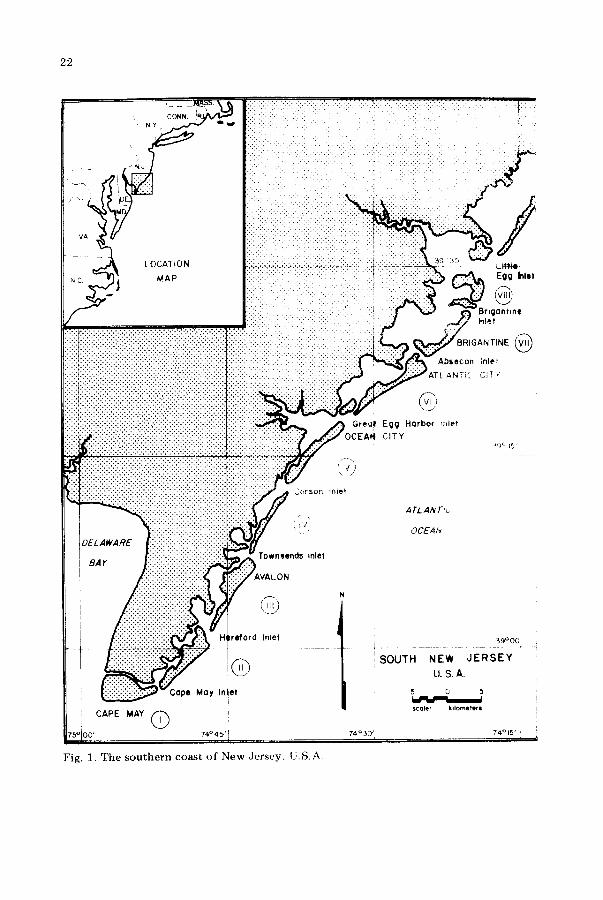
The Atlantic coast of North America is one of the world's most dynamic sedimentary environments. Extratropical and tropical storms generate waves and surge that frequently alter the subaqueous and subaerial portions of the shore zone. During the past several decades there has been a net trend toward coastal recession (erosion) along the Atlantic coast. This trend has been attributed to a recent rise in sea level (Bruun, 1962; Hicks and Crosby, 1974), a reduction in new fluvial sediments (Wolman, 1971), human altera- tions of coastal morphology (Dolan, 1972), and secular changes in storm fre- quencies and magnitudes (Hayden, 1975). Changes along New Jersey (Fig. 1) are typical for the Atlantic coast; the average rate of recession is about 1 m/yr. This paper summarizes a new method of recording shoreline changes over extensive reaches of sedimentary coasts using aerial photography and an orthogonal grid system. A 90-km section of the New Jersey coast is used for a demonstration project.

22

, _ ..

,CONN. N.Y

LOCATION

MAP

:.:......

• . - : , + : . : : : : : . . : . .

" : : : : / ' : :-/. : . : , :::.:.." .:-:-:t. " : : : ' : : • . '"

:!I

. . . . . . . . . . .. .

!i!ii ~; • . i : : : : : : : / :: : ' ::::::::::::::::::::::::::::::::::::::::::::::::::::::::::::::::::: . . . . ~i:i:i:~:!:i:~iii~!!i~i~iiiiiii~i!iiiii!i~i~i~!~i!i~!!i!ii~:!i~i~iiiii!~iii~i::!::i~:

i iiiiiiiil;iiiiiiiiiiiii!ii!iiiiiii!i!iiiiiiiiiiiiii" ,iiiiii!i!iiiii!ii~:i~!:::ii:~:!! ::::::::: "::::::- :. . : , ..... • . , . . . . ,

:;221:2:::2::2:::.:.22. .: : -

?ii!iiii iiiiiiiiiiiiiiiiiiii!iii:i!i ii iiii ;! ili • . . . . . . . . . . . . . . . . . . . . . . . . . . . . . . .

~:?~?~ii~!~i~!i!i!i!i!~!i!?i!!21iiiiiiii~iiiii!iiiiiiiii!!ili:::: . . . . . . .~ . -'. :::-'-'.'::- -'.:-:.:.:.:-:-:'i':

i "".,...i. ',. ' .,".', '-2.:-i-

. . . . .... iii??iiii??iiii)iiiiiii!ii)i!? =========================== ??!i"" . . . . . . . . . . . . . . . . -.-.,... :.:.:,:.:.:.:,..,.......,-,-.-.........-....:-:-:.::::::.:.:,:.:.:

/ L.;I; '¢'. E g g Inlet

.~ grlgonhne v Inlet

~IGAN TINE @

. . . . . .-. ! i i S # COF~,On Ir~iet

iiiiiiii ii S / i ! . 1

o ~ . ~ , ~ ::::::i::i::i~i~iii::i::i::i::!~i::i~i::ii::i . 0 . ° . ° 0 . , ° , 0 , BA Y

iii!i!::')AVA L ON

.... i:!:i:i:i:i:i ",'~ "- ' "

~... ,.. .:!:!:i:i:!:!:i:i:i:i:?:i:i :~ei'0( ~a I.~t

! CAPE MAY ~ ! LL~

Fig. 1. The sou the rn coas~ of New Jersey, L!.S.A.

Absecon inlet

ATL ANTIC 's~r

E g g H a r b o r ;~lel

C I T Y

A T L A N T c~

0 CEA/v

39°001

'SOUTH NEW JERSEY U.S.A.

scale: k11ometer$ !

74 ° 301j 74015" i i

23

DETERMINING TRENDS IN SHORELINE EROSION AND DEPOSITION

Along the Atlantic coast, storms cause landscape modification at a wide range of scales. Private land holdings are destroyed, communication and transportation facilities are disrupted, and the loss of life is not uncommon. In spite of these obvious problems in coastal areas where extreme storms are common, with few exceptions management strategy has been based on the concept that the landscape is stable or at least that it can be engineered to remain stable.

To marine scientists, managers, and coastal engineers the shoreline and beach-face have long been recognized as elements of a highly dynamic sys- tem. The information base needed for good planning and engineering design includes the current state of the system and rates of change through time. Information of this type can be obtained: {1) by ground surveys; (2) from maps and charts; and (3) from aerial photographs.

Ground survey methods provide data of the highest resolution but accurate historical records that can be used for comparisons are lacking for most coastal areas and the generation of new surveys is expensive and time consuming. With the exception of a few scattered sites, ground information is generally unavailable.

Maps and charts are available for numerous coastal locations and frequent- ly extend back to the mid-1800's; however, while charts are useful, most are of questionable accuracy and are frequently restricted to areas immediately adjacent to major shipping lanes and port facilities. Maps and charts best serve as supplemental information in determining historical trends in shore- line change.

Aerial photographs, taken with metric mapping cameras, are available for most coastal locations in the United States. Earliest photographs date back to the 1930's or early 1940's, and photographs for subsequent decades are generally available.

Aerial photography has many advantages over the other types of informa- tion in coastal mapping. In a matter of hours hundreds of miles of coast can be photographed: an instantaneous record rather than a survey spanning months or years. Photographs include a measure of detail over extended areas unavailable with any other information base, and they are permanent and easily duplicated.

While aerial photographs are usually taken with high resolution metric cameras, they are not the equivalent of maps. This lack of orthogonai equi- valence" results in scale variance within and between images. Scale variations are generally of four types: (1} differences caused by changes in the altitude of the camera platform; (2) variations due to camera tilt; (3) radial scale variations away from the image center; and (4) distortions due to relief variations of the surface photographed.

The scale variation due to land relief is the least serious error along low sedimentary coasts, resulting in insignificant errors in measurements (Staf-

24

ford and Langfelder, 1971), and radial scale distortion is also well within the potential error associated with mapping shoreline changes. Tilt error within images and scale error between images is usually minimal and is easily rectified using correcting enlarging projectors.

Early at tempts to obtain information from aerial photographs focused on the identification of coastal landforms (Lucke, 1934); illustration of coastal processes (Eardley, 1941; Shepard et al., 1941), and the classification of coastal features (Smith, 1943).

In 1947 McCurdy identified the high water line (HWL) as a major recogni- zable feature of the subaerial beach face. Later, McCurdy (1950) and McBeth (1956) indicated that there was only an insignificant difference be- tween the water line of the previous high tide and the HWL line recognized on photographs. The stable nature of the HWL over a tidal cycle was later confirmed by Stafford (1968). During the 1950's several at tempts were made to assess beach erosion with aerial photographs (Rib, 1957; Zeigler and Ronne, 1957; Chieruzzi and Baker, 1958). In 1960, Williams recommended several procedures to insure accuracy in extracting information from aerial photography, and subsequently Tanner (1961) at tempted to calculate from a sequence of aerial photographs changes in beach sand volume caused by storm action.

Efforts to quantify local shoreline changes using aerial photography in- creased following the great Atlantic coast Ash Wednesday storm of March, 1962 (El Ashry, 1963; Athearn and Ronne, 1963; Harris and Jones, 1964}. Larger coastal reaches were investigated subsequently by Plusquellec (1966), Gawne (1966), and E1 Ashry (1966), using common scale planimetric maps generated from aerial photo interpretation. Shoreline change measurements were made by Stafford (1968), Stafford and Langfelder (1971) and Lang- felder et al. (1968, 1970). They also assess the errors inherent in metric aerial photographs as well as errors in their interpretation.

The shoreline

The simple definition of a shoreline is the edge of a body of water; how- ever, the position of the shoreline on the beach face is highly variable because of changes in water level due to lunar tides, waves, and wind tides.

The slopes on the beaches along the mid-Atlantic coast vary from 1 : 10 to 1 : 50. With a tidal range of approximately 1.0 m to 1.25 m the intersec- t ion of the beach and ocean has a horizontal variation range over the tidal cycle of 10 m to 60 m for 1 : 10 and 1 : 50 slopes, respectively (Fig. 2). This level of variation of the shoreline interface is unacceptable for a mapping program designed to characterize changes in the shoreline over several decades. Two alternatives are available: (1) correct all data sets for tidal stage at the time of the flight of the photography; or (2) define some other more stable marker of the shore which is less sensitive to tidal stage. In these studies the latter strategy was followed -- the alternative is the high water line as seen on the photography.

25

HIGH WATER L INE AND

' . . . . . . " i-?.. :,. / RANGE • : ' . °" :°'~.. . . [ - ~ - ~ ,, . . . .

~ ~ : . ' ; . ' . ~ . : ~ _ . ~ : .

o , , ~ X E , a ~ ° ' \ , m . TE,,I ,UG I ":" ".I:~.".'-";"..'.:.:~..~._ - I ~ >l • ".." " " : " " : : " " ' .

• .. - : . . . . " ~

Fig. 2. Hor izonta l d i sp lacement of high water line vs. swash terminus .

For the purposes of shoreline recognition on aerial photographs, the major requirements are: (1) that the shoreline be easily and consistently recog- nizable on both black and white and color imagery; (2) that it be linearly continuous along-the-beach; and (3) that the across-the-beach variations in position due to changes in water level be at a minimum.

Nine possibilities were assessed (Table I); only the high water line was favorable for all criteria.

The high water line is re-established with each high tide as the upper beach is wetted. The resulting boundary between moist and dry sand is evident on

TABLE I

Criteria for shorel ine se lect ion

Possible operat ional Criteria for shorel ine select ion.* shorel ines 1 2 3

Line of inshore bars no no yes Mean low water no yes yes B o t t o m o f swash zone yes yes no Mid-swash zone yes yes no Swash te rminus (ST) yes yes no Mean sea level no yes yes High water line yes yes yes High t ide line no yes yes Berm line no no yes

"1 = Tha t the beach-face feature (shorel ine) def ined be easily and cons i s ten t ly recog- nizable on bo th black and whi te and co lor IR imagery; 2 = tha t the feature be linearly con t inuous a long-the-beach ; 3 = tha t the across- the-beach variations be at a min imum.

26

both color and black and white aerial photography as a distinct tonal change (Fig. 3).

High water line (HWL)

Variations in position of the HWL during the lunar tidal cycle, as recog- nized on aerial photographs, are of two types: (1) up-beach movement

~:~.~ ......

Fig. 3. Cu r r en t h igh wa te r l ine as seen on b lack and whi t e ob l ique aerial p h o t o g r a p h .

associated with the rising tide; and (2) down-beach movement forced by drying of the sand surface. At the time of high tide, the swash terminus (ST) and HWL are the same (Fig. 2); as the high tide falls both the ST and HWL migrate seaward. The HWL migrates much slower, however, than the ST. The extent of the horizontal displacement of the ST is a funct ion of the slope of the beach, the tidal range, roughness of the beach face, and the wave height and period at the time of wave runup. In addition, occasional variations in water level due to longer period tidal components , storm surges and wind set-up and set-down may fur ther increase the horizontal displace- ment. The extent of the horizontal displacement of the HWL landward is a funct ion of the same factors, since on the rising tide, the HWL equals the ST. But the horizontal displacement of the HWL seaward during the falling tide has the additional factor of drying the beach sand. The drying process retards the seaward movement of the HWL, and it never retreats as far as the ST. Thus, the HWL has a smaller horizontal displacement than the ST and is, therefore, a more suitable choice for the shoreline.

27

STORM SURGE PENETRATION (VL)

During periods of extreme storm activity (high waves and/or wind surge) low lying coastal areas may be f looded and overwashed by sea waters. The overwash is a bore of highly turbulent, sediment-laden water which moves across the beach and onto subaerial portions of the coast. As this f low moves inland, its velocity is reduced so that at some point the flow of water can no longer transport sediments. Thus a zone of sediment transport is produced between the beach and the line of inland penetration of the bore: the zone of overwash deposit.

In the months immediately following an overwash event the newly deposited sand is clearly evident against the contrast of vegetated or developed surfaces. As time passes, vegetation encroaches on the sand deposit and the overwash zone begins to narrow. Thus there are two separate processes that give definition to the width of the overwash penetration zone: (1) overwash events that widen the zone; and (2) vegetation regrowth that narrows the zone.

The width of the overwash penetration zone is defined as the distance be- tween the shoreline and the line (VL) of encroaching vegetation (or develop- ment) on the overwash deposit.

The width of the overwash zone is variable over time and the magnitude of this variability also changes along-the-coast. Along the Atlantic coast areas that experienced deep overwash penetration in the 1940's usually experi- enced deep penetration in the 1950's, 1960's and 1970's.

Measurement o f shoreline and storm penetration

There are several methods available to coastal investigators to determine historical trends in shoreline change. These range from highly accurate engineering surveys to very general patterns detected by comparisons of old photographs. The paragraphs that follow summarize the advantages and dis- advantages of the "s tandard" methods.

Accuracy:

A d van rages:

Repeated shoreline surveys Cost: Data acquisition based upon field survey is very expensive

because of the high man hours required. Survey data are the most accurate available with resolu- tion on the order of 0.01 m or less. (1) Measurements are direct. (2) Individual measurements may be updated at relatively moderate cost. (3) Measurement method commonly understood by the public. (4) Measurement commensurate with local property sur- vey records.

28

Disadvan rages: (1) Historical timeline of data usually not available. (2) Accuracy of measurement greatly exceeds the resolution of shoreline definition. (3) Along-the-coast data density is poor. (4) Systematic updating of extensive coastal reaches would be very expensive and time-consuming. (5) Because surveying is time-consuming, measurements differ markedly with sea state conditions.

Accuracy:

Advantages:

Disadvantages:

Metric aerial photography Cost: Given the along-the-coast density of available data the cost

is rated as low. Resolution of data varies with scale of photography, normal errors are less than 5 m. (1) High along-the-coast resolution. (2) Historical data for the last 40 years usually available. (3) Data is highly time-specific. (4) Shoreline definition is within the resolution error of systems being analyzed. (5) Repeated coverage is inexpensive if extensive coastal areas are included. (6) Frequent coverage in time generally available. (1) Longer time lines than the last 40 years are generally not available. (2) Photointerpretat ion skills needed to reduce data. (3} Variation in photography type may result in errors. (4) Some historic photo series are classified and not available for general use.

Historic maps and charts Cost: Map and chart derived data are generally inexpensive but

cost associated with data to produce original maps is high. Accuracy: Map accuracy is generally unavailable but may be

estimated in the tens of meters. Advantages: (1) Maps and charts from the mid-1800's are available in

the USA, thus providing an unusually long time frame for determination of mean shoreline erosion.

Disadvantages: (1) Irregular availability. (2) Unstable map bases. (3) Low accuracy and resolution. (4) No correction for sea state or tide level.

Property survey and tax maps Cost: Where available, such data are inexpensive.

29

Accuracy:

Advantages:

Disadvantages:

In general, such maps are as accurate as field survey, but definition of the shoreline is rarely defined in a systematic way and therefore errors may be on the order of tens of meters. (1) Availability for most commercial and residential areas. (2) Map base understood by public at large. (1) Historical survey and tax maps are in general un- available. (2) Poor shoreline definition. (3) Systematic updating unrealistic.

Non-metric photography (hand-held cameras) Cost: Data is generally inexpensive. Accuracy: At best, accuracy is poor with little information about

either sea state or tide cycle. Advantages: (1) Historical information is possible. Disadvantages: {1) No systematic archives of such information is available.

(2) Photos are almost always oblique views requiring ex- tensive correction. (3) Scale is usually difficult to estimate.

THE ORTHOGONAL GRID ADDRESS SYSTEM (OGAS)

The analysis of shoreline dynamics for the purpose of specifying rates of erosion and coastal hazard zones requires repetitive sampling of the coastal system, both spatially and temporally. Review of the methods available leads to the conclusion that the use of metric photography is the only feasible solution to a regional or nation-wide mapping effort. The Orthogonal Grid Address System (OGAS) method has been designed to meet these needs.

In essence, the method provides for the rapid and systematic acquisition of shoreline and storm penetration information from historical aerial photo- graphs at 100-m intervals along the coast. Comparison of the data derived from different years permits the definition of statistical properties of the coastal data sets.

Base maps

Prior to the interpretation of historical aerial photographs, standard 1 : 5,000 scale base maps of the study region are prepared. These base maps are produced by photo enlargement of 71A minute series USGS maps (1 : 24,000). Each base map represents an area 3,500 m by 2,100 m. The frame of each base map is oriented with long side parallel to the coastline and positioned over the active portion of the coast. The long axis, lying entirely over the ocean, is the baseline from which all measurements are made (Fig. 4).

30

USGS TOPOGRAPHIC MAP S C A L E - 1 :24 .000

1. Enlarge blaemap f rom topo map.

2 . Draw ihore l ine and vegetat ion l i ne f rom photograph.

, Measure d is tance of shoreline and vegetat ion l i ne f r o m h l l l l i n e , w i t h gr id over lay,

LOW ALTITUDE PHOTOGRAPH SCALE -- I : 20 ,000

&

OVERLAY 1 : 5 ,000

Fig. 4. Method of data collection.

Photo projection

The historical aerial pho tog raphs are then enlarged to the exac t scale of the base map by p ro jec t ion o n t o the base map. On a t r ansparen t overlay p laced on the base map, the shorel ine (HWL) and active sand zone line ( s to rm pe ne t r a t i on line) are t raced f rom the p ro jec t ion (Fig. 4). Such tracings p repared f rom 1 : 5 ,000 scale p ro jec t ions of a sequence o f historical pho tog raphs cons t i tu t e the raw car tographic da ta base f rom which subse- q u e n t measu remen t s are ex t rac ted .

31

Grid addressing and data extraction

On each photographic tracing a transparent grid is overlaid -- the grid is rectilinear with 100-m spacings. Any coastal location is thus specified by base map number and co-ordinates of the 100 × 100 m grid. The position of the shoreline and other lines of interest, with respect to the base map base line, are then measured to the nearest 5 m with a high-resolution movable cursor grid. These data are punched on IBM cards for subsequent analyses.

Computer printout of OGAS

The data contained in our OGAS output represent s the location and change in location-over-time of the storm penetrat ion line (VL) and shore- line (SL) on transects positioned at 100-m intervals perpendicular to the trend of the shoreline. The data source for our New Jersey demonstrat ion was aerial photography for the following time periods: 1930, 1940, 1949, 1962, and 1971. As indicated earlier, the shoreline (SL) is defined as the high water line. The storm-surge penetration line (or vegetation line, VL) is defined as the line that separates the active, non-vegetated or non<leveloped sand areas (including non or sparsely vegetated sand dunes which show evi- dence of overwash penetration), from the areas of continuous stands of grass and shrub (including grass-covered dune masses that show little or no evi- dence of overwash penetration or development). In absence of such a vegetated or developed area, the VL in the barrier island case is defined as the bay shoreline. The values on the OGAS computer printouts for VL and SL represent the distances to the VL and SL, in meters, from the map base line located over the ocean and running parallel to the trend of the shoreline. Also listed is the storm-surge penetration distance or overwash penetration (OP). This represents the width of the active sand zone between the shore- line and the line of development or the vegetation line, and is calculated by subtracting the value for SL from the value for VL (Fig. 4).

The New Jersey coast is divided into map sections of 3.5 km in length, with a base map associated with each section. Each OGAS base map contains 36 transects, spaced 100 m apart. Each transect is identified by a map and transect number (M-TR). Thus, any point along the coast can be located to the nearest 100 m.

The computer program presently in use provides data ou tpu t divided into 11 sections of tables and graphs. Tables are valuable as a permanent histori- cal data bank; the graphs are most useful stretched out and spliced together for visual analysis. For each set of dates over all maps, changes are calculated, listed, and graphed for time periods between adjacent dates and between the first date and the last date.

The mean + one standard deviation of rate of change of the shoreline and the storm penetration line are the most useful for determining areas of the coast which have been subjected to the greatest extremes of change (Fig. 5).

32

• N(AN eAV~ Or CHAN6E, ~RO. 0ZJUW]8 IC 6 ~ J U N I ~ ( ~ . O 0 VEA~S) . S ONE $1&N~&~O D E V I A T I O N r~ON THE NEAN. • = ~£AN EN~ $ laNDEqO 0 E V I I T T O N WERE C&LC.JLATE0 OVeR i TOTAL t I f f E PERIOD LESS THAN 3 E . 0 { ¥~.ARS 0UWE To ABSENCE O F ~)&t&. N ITR = i'q&P 4~3 TRENSECT HUMBER* ~AGH TQSNSECT REPQESEWTS A rJXST&NGE OF 1~0 NETE~$ ALONG THE GC)ASK,

A C C R E T I O N -- EEAWARO MIGRATION 4 G • ERO61ON - LANDWARD MIGRATION

~ / r e S"OQELINE ~A~'~ o~ CH*WGE ~CRO$$ T,E CO*ST I N METEI~$/VE*~ ~ / T R M~AN $ . D * ONOER°WT. -WE. -wO. - 3 5 . - ] 3 . - ? 5 . - E ; . - 1 5 . - 1 C . -$o ~.O 5° 1~. 15 . Zd . Z $ . $0o 15o ~0 . ~ 5 . x .OVER ~S

S I , s 3 . 3 ~ . 2 S [ e $ 3 .1 (+.k s I , s ] . z ~ . E

s I . s z . ~ 6.b 16- $ S IM S 1 6 - 5 1 . 4 6 , 5

s I n s ~ . s 6 . s s : . s 1 . o r ,C

s I , s 1 , q ~.'~ s I M s z , o a , o

t E - I 0 S I ~ S 1&-10 Z , l 8 ° ] s I . s ~ . z ~ . I

s I , s 2.4 ~.~ s I , s 2 . e r . e

I ~ - t 5 S I ~ s z b - t ~ ~ . I 6 . 9 $ I ~ s ] . 3 + . ~

s t s ~.7 s . o s I s ~ , 7 W.4

16-~O sl s l~ , -?~ ) . ~ 4 , 5 Sl s .~,7 ~.s

s ~ s s ~+z 5 .S

s s ~ .s ~ . 6

s I ~ s I . a 6 .a s I , s ~ , t P . z s I ~ s ~.~ ~.*

s I ~ s s I s ] , ' ; ~.o

s I s ,,z z x . z UNDER-45, +~5* -~52. - J ~ . - ] ] . - 7 5 . -?D. - 15 . -1C. - 5 . o . e s . t o . 15. 2~. ?s. $ C . I5. 4d. . 5 . ~ " .Ov t~ ~5

S I S + . z t l , ~ s z s ~.z ~ z . z

; I s s ~.~ Iz,'+

s 1 s ~.~ I 0 . 6 I s s . t % r

I s I s ~.3 ~ . e I P - I O s I s zz+zo s . ~ s . o

s r . ?

sz s s . ~ s . ~ s I s ~ . t r . 1

s r s ~ . 5 ; ' , b s I s ~,~s ~ . 6 s I s ~.~ ~ . ~

E7-~0 S I S I ? - Z { 1 , 3 a°?

s I s s I s ~ . q ~ I . 9

s I s ~+1 1 ~ . + Ir-3o s I s 1 7 - ] 6 + . ] l e . ~

s I : :+.{I ?b.~ 1X-75 I s : E l - I s ZC, mZ Z ~ . 5

61 s s • : q.w ] . + ONO~-k~ . -wS. - 4~ . - 5£ . - 3 . . - 2 5 . - 2J . - 15 . -1C. - 5 . .~ 5. 1C. 15. ~e. ZS. ~(] , ~5, k ) . ~5. • .ovE~ ws

S I S : z ~ , , , ? w . r

I s , ~ . q I , m

S I S I 1 . 1 } ~ . S S I I I . Z 30,6

s I S L I , W ZS.B s • s 1 1 . 4 ~o.~

S I S 1 1 , 4 1~ .3 ; I ; I I m ~ 12 • ~

s s s I ~ . ] 1 1 , ~

l ] m I } I S $ I I & - 1 5 I 1 . C L~,Z I IS s l ~ . r L O . X

Fig 5. Graph showing mean rate of change of shoreline -+ one standard deviation.

It v isual ly presents a measure o f shore l ine variabil i ty and gives an indica- t i on o f the m o r e stable versus the m o r e vulnerable parts o f the coast l ine . The standard dev ia t ions ca lcu lated , whi l e based u p o n o n l y f ive sets o f p h o t o - graphy, were f o u n d to be h ighly u n i f o r m a long the coas t . N u m e r i c a l va lues

33

for mean and standard deviation at each transect are listed. The standard deviation lines that form an envelope on each side of the mean are of great value because they are a combination of the historical trend of mean change and of episodically occurring extreme storm events.

THE NEW JERSEY COAST

A demonstrat ion of the applicability of this newly developed shoreline erosion and storm penetration measurement system was carried out along the New Jersey coast from Cape May to Little Egg Inlet, a distance of 90 km (Fig. 1). This section of the coast is not an unbroken reach of straight shore- line .... it is segmented, however, into eight individual "islands" by a series of inlets. For this reason we have divided our discussion into an island-by-island treatment.

Fig. 6 shows the generalized trends of shoreline change for the eight indi- vidual segments making up the 90 km of the New Jersey coast. The wide range of shoreline dynamics suggested by these along-the~oast patterns is clear justification for not treating the 90 km of the coast as a single unit. In fact, one could even question generalizations on an island-by-island basis. Again, Fig. 6 helps evaluate this problem. Islands IV and VI have very low variance along the coast so the averages of shoreline erosion and storm pene- tration are good estimators. In extreme contrast, mean rates of erosion for island VIII would give poor estimates because the along-the-coast variation is is very high and the mean statistics would be representative of but a small port ion of the island. Islands II and VII also have high variances; islands III and V have modest variation. Thus it is clear that island means are not necessarily the best choices for planning, design criterion or establishing risk and hazard zones for programs such as the Federal Flood Insurance Program.

The eight New Jersey islands

The shoreline at the southern end of New Jersey from Cape May Point to Cape May Inlet (Island I, Fig. 1) has eroded at an average rate of 3 m/yr. This rate has been constant during the 41 years from 1930 to 1971. The storm-surge penetration line for this reach has receded at the rate of 2.7 m/yr. The average width of the active sand zone was 60 m over 41 years, and ranged from a low of 21 m in 1949 to a high of 159 m after the Ash Wed- nesday storm in 1962. At one location near Cape May, the overwash penetra- tion was 425 m as a result of the storm of March, 1962.

The coast of Wildwood from Cape May Inlet to Hereford Inlet (Island II, Fig. 1) has responded very differently to coastal processes when compared with the section south to Cape May. Both the shoreline and the overwash penetrat ion line showed a net accretion of approximately 1 m/yr since 1930. The variability in change over time was moderate and fairly uniform along the beach. The average width of the active sand zone has remained unusually stable both temporally and spatially at just above 150 m.

34

0 I Z 3 4 5

HORIZONTAL $~LLE: KILTERS

~ BRIGANTINE INLET TO LITTLE EGG INLET o VI I I

- - - i o

BSECON INLET TO BRIGANTINE INLET

=~ 5 L GREAT EGG HARBOR INLET TO ABSECON INLET =

o I . . . . . . ~ " " ' : " : " " . m , Vl

5 / OR O. ,NLET TO GRE,T EOG o ~ - ~ - - ~-~-~:~i: v

J W

r r TOWNSENDS INLET TO CORSON INLET [ 5

5

0

z - 5 0 5

HEREFORD INLET TO TOWNSENDS INLET

CAPE MAY INLET TO HEREFORD INLET

CAPE MAY POINT TO CAPE MAY INLET

0

( S O U T H . . . . ALONG T H E C O A S T . . . . N O R T H

I

>

Fig. 6. Generalized trend of shoreline change for the eight barrier islands of southern New Jersey.

From Stone Harbor to Avalon between Hereford Inlet and Townsends Inlet (Island III, Fig. 1) the pattern of change is similar to that in the Cape May section. The shoreline is more stable with a mean rate of erosion of 0.7 m/yr and low variability, both spatially and temporally. The overwash pene- tration line is relatively low, 1.4 m/yr recession, because of massive engi- neering works, including sea walls and groins.

In the period from 1930 to 1971, the 11 km section of coast from Townsend Inlet to Corson Inlet (Island IV, Fig. 1} experienced erosion rates of 2.5 m/yr and overwash penetration recession of 2 m/yr. The spatial varia- bility was very low in both cases, with a standard deviation less than 1.5.

35

Furthermore, the temporal variation of the shoreline was very low. The shoreline from Corson Inlet to Great Egg Harbor Inlet including

Ocean City (Island V, Fig. 1) has been stabilized by engineering works since 1930. Unlike the islands to the south, the Ocean City shoreline showed a net accretion of 26 m from 1930 to 1971, for a rate of 0.6 m/yr. This stability and minimal amount of shoreline change can be attributed in part to the extensive system of groins and sea walls on the island. The average width of the overwash penetration zone during the period 1930 to 1971 was 80 m. This nearly tripled to 217 m following the Ash Wednesday storm of 1962.

The most notable features of the coastline between Great Egg Harbor Inlet and Absecon (Island VI, Fig. 1), are its extreme vulnerability at Margate City and its extreme stability at Ventnor City and Atlantic City. The net rate of change in the overwash penetration line along this 13 km is- land was 0 m/yr between 1930 and 1971. Due primarily to the Ash Wednes- day storm of 1962, however, the standard deviation of the rate of change of this line as measured from the five sets of photography exceeded 40 m/yr in Margate City. In Ventnor and Atlantic cities, the maximum standard devia- tion was 5 m/yr. Stated in other terms, the extent of storm surge penetration in Margate City due to the Ash Wednesday storm was as great as 670 m; whereas in Ventnor and Atlantic cities, the penetration seldom exceeded 100 m. The net average change in shoreline in 41 years was 27 m accretion (0.7 m/yr).

Approximately half of the shoreline between Absecon Inlet and Brigan- tine Inlet (Island VII, Fig. 1) is developed at the town of Brigantine. Although there are numerous groins, very little of Brigantine Beach is pro- tected by a sea wall. The shoreline has experienced an average net accretion of 0.6 m/yr since 1930. This has, however, been highly variable. For example, a 1-km stretch of shoreline in Brigantine has been eroding at a rate of 3 m/yr; whereas the southern 2 km of the island have been accreting as much as 12 m/yr since 1930. The net change in the overwash penetration line has been seaward at a rate of 1.6 m/yr since 1930.

The 4-km section of coast between Brigantine Inlet and Little Egg Inlet (Island VIII, Fig. 1) is entirely undeveloped. The shoreline at the northern half of the island has accreted at rates higher than 30 m/yr from 1930 to 1971, while that at the sourthern half is eroding at rates in excess of 20 m/yr. The overwash penetration distance is greater than anywhere along the southern New Jersey coast, averaging 333 meters over the time periods studied.

Summary of hazards for the New Jersey islands

Along the New Jersey coast the shoreline and storm-surge penetration line covary in areas that have not been stabilized by engineering works. The mean rates of shoreline change and changes in the storm-surge penetration line for each of the 8 New Jersey study islands are plot ted in Fig. 7. The nearly

36

5

4-

3-

/ I

2 S I

vI -~ -~ -~ - , , ~

,viii

O ACCRETION ~ ~ ,~ EROSION u~ SHORELINE MEAN RATE OF CHANGE (m/y r )

Fig. 7. Scatter plot of mean rate of change in shoreline vs. storm-surge penetration line for eight barrier islands in southern New Jersey.

linear fit of the points clearly indicates that the zone of storm-surge damage is rather constant in time and space. As the shoreline erodes, the storm-surge penetration line likewise recedes. This relationship is of practical significance because coefficients for insurance rates based on hazard probabilities would apply equally well to both erosion and storm-surge hazards.

It is also of interest to note that the standard deviations of rate of change in shoreline and storm-surge penetrat ion line likewise covary (Fig. 8). That is, areas of highly unstable shoreline, with large excursions of the shoreline in the erosive and accretive directions, are also areas with similarly large varia- tions in location of the storm-surge penetration line.

CONCLUSIONS

Detailed information on shoreline dynamics is required by coastal engineers, planners, and in the United States, for various sections of the National Environmental Policy Act of 1969, Coastal Zone Management Act of 1972 with 1976 amendments, and the Flood Disaster Protection Act of 1973. Since there is no program for systematic data collection in the United

37

~ ..E.E 14-

I z l 2 - iE ' r

~ IO-

u. uJ 8 ~

z 6 - O w

~ J 4

, ~ a : 0

z ~ J , ~ z F - w m n

j , , J J _ J Y=.59 X -'1- 1.81

, ~ r= .94

"ely eVl

o 2 ~, ~ d ,b ,~ ,:4 J~ ,8 2'0 2'2 STANDARD DEVIATION OF SHORELINE RATE OF CHANGE ( m / y r I

Fig. 8. Sca t t e r p lo t o f s t a n d a r d devia t ion of ra te o f change in shore l ine vs. s torm-surge p e n e t r a t i o n l ine for e ight barr ier is lands in s o u t h e r n New Jersey.

States to provide this information, existing historical data must serve as the base. Of the available types of historical data only aerial photography pro- vides a record with sufficient spatial and temporal detail for a national mapping program. The orthogonal grid address system described in this paper is designed to maximize the usefulness of the existing imagery. Finally, this research has led to the conclusion that an annual photographic record of all sections of the U.S. coastline is essential for research, planning, and shore- zone management.

A C K N O W L E D G E M E N T S

We wish to give special acknowledgement to our research assistant, Ms. Kathy Schroeder, who performed the aerial photograph interpretation for the historical erosion and storm-surge penetration data. The research was made possible through funding from the Department of Housing and Urban Development, NASA-Goddard Space Flight Center, and the National Park Service. Aerial photography for the New Jersey study was provided by the New Jersey Office of Shore Protection. Finally we wish to thank the Chesa- peake Bay Ecological Program Office for providing services and imagery essential to the development of our method of measuring coastal change.

REFERENCES

Athearn, W.C. and Ronne, F.C., 1963. Shoreline change at Cape Hatteras: an aerial photographic study of a 17-year period. Naval Res. Rev., 17(6): 17--24.

Bruun, P., 1962. Sea-level rise as a cause of shore erosion. J. Waterways Harbors Div., 2-15.

38

Caldwell, J.M., 1959. Shore Erosion by Storm Waves. Misc. Pap. No. 1-59, Beach Erosion Board, Office of the Chief of Engineers, Department of the Army Corps of Engineers.

Chieruzzi, R. and Baker, R.F., 1958. A Study of Lake Erie Bluff Recession. Bull. 172, Eng. Exp. Stat. Ohio State Univ., Columbus, Ohio.

Dolan, R., 1972. Barrier dune system along the Outer Banks of North Carolina: a reap- praisal. Science, V (176): 286--88.

Eardley, A.J., 1941. Aerial Photographs: Their Use and Interpretation. Harper, New York, N.Y.

E1-Ashry, M.T., 1963. Effects of Hurricanes on Parts of the United States Coast Line as Illustrated by Aerial Photographs. Unpublished Master's Thesis, Department of Geology, University of Illinois, Urbana, Ill.

E1-Ashry, M.T., 1966. Photo Interpretation of Shore Line Changes in Selected Areas along the Atlantic and Gulf Coasts of the United States. Unpublished PhD Thesis, Department of Geology, University of Illinois, Urbana, Ill. University Microfilms, Ann Arbor, Mich.

Gawne, C.E., 1966. Shore Changes of Fenwick and Assateague Islands, Maryland and Vir- ginia. Unpublished Senior Thesis, College of Liberal Arts and Sciences, University of Illinois, Urbana, Ill.

Harris, W.D. and Jones, B.G., 1964. Repeat mapping for a record of shore erosion. Shore Beach, 32(2): 31--34.

Hayden, B.P., 1975. Storm wave climates at Cape Hatteras, North Carolina: recent secular variations. Science, V(190): 981--983.

Hicks, S.D. and Crosby, J.E., 1974. Trends and Variability of Yearly Mean Sea Level. NOAA Tech. Memo NOS 13, National Oceanic and Atmospheric Administration, National Ocean Survey, Rockville, Md.

Kraft, J.C., 1971. Sedimentary facies patterns and geologic history of a Holocene marine transgression. Geol. Soc. Am. Bull., V(82): 2131--2158.

Langfelder, J., Stafford, D. and Amein, M., 1968. A reconnaissance of coastal erosion in North Carolina, Project ERD -- 238. Department of Civil Eng., North Carolina State University at Raleigh, 126 pp.

Langfelder, J., Stafford, D. and Amein, M., 1970. Coastal erosion in North Carolina. J. Waterw., Harbors Coastal Eng. Div., WW2, pp. 531--545.

Lucke, J.B., 1934. A study of Barnegat Inlet, New Jersey and related shore line pheno- mena. Shore Beach, 2(2): pp. 98--111.

McBeth, F.H., 1956. A method of shore line delineation. Photogram. Engr., 22(2): 400--405.

McCurdy, P.G., 1947. Manual of Coastal Delineation from Aerial Photographs. U.S. Navy Hydro Off. Pub. No. 592, U.S. Navy Hydrographic Office, Washington, D.C.

McCurdy, P.G., 1950. Coastal delineation from aerial photographs. Photogram. Eng., 16(4): 550--555.

Milliman, J.D. and Emery, K.O., 1968. Sea levels during the past 35,000 years. Science, V (162): 1121--1123.

Plusquellec, P.L., 1966. Coastal Morphology and Changes of an Area between Brigantine and Beach Haven Heights, New Jersey. Unpublished Master's Thesis, Department of Geology, University of Illinois, Urbana, Ill.

Rib, H.T., 1957. The Application of Aerial Photography to Beach Erosion Studies. Un- published Master's Thesis, Department of Civil Engineering, Cornell University, Ithaca, New York, N.Y.

Shepard, F.P., Emery, K.O. and LaFond, E.D., 1941. Rip currents: a process of geological importance. J. Geol., 49(4): 337--369.

Smith, H.T.U., 1943. Aerial Photographs and Their Application. Appleton-Century- Crofts, Inc., New York, N.Y.

Stafford, D.B., 1968. Development and Evaluation of a Procedure for Using Aerial Photo- graphs to Conduct a Survey of Coastal Erosion. Report prepared for the State of North Carolina, Dept. of Civil Engineering, North Carolina State University, Raleigh, North Carolina. (Also unpublished PhD Thesis).

39

Stafford, D.B., and Langfelder, J., 1971. Air photo survey of coastal erosion. Photogram. Eng., V (37):565--575.

Tanner, W.F., 1961. Mainland beach changes due to hurricane Donna. J. Geophys. Res., 66(7): 2265--2266.

Williams, W.W., 1960. Coastal Changes. Routledge and Kegan Paul, Limited, London. Wolman, Gordon M., 1971. The nation's rivers. Science, V (174): 905--918. Zeigler, J.M. and Ronne, F.C., 1957. Time-lapse photography - - an aid to the studies of

the shoreline. Naval Res. Rev., (4): 1--6.