A New Parallel Algorithm for Simulation of Spin-Glass ... · the following time-correspondences...

Journal of Modern Physics, 2011, 2, 488-497 doi:10.4236/jmp.2011.26059 Published Online June 2011 (http://www.SciRP.org/journal/jmp)

Copyright © 2011 SciRes. JMP

A New Parallel Algorithm for Simulation of Spin-Glass Systems on Scales of Space-Time Periods of an

External Field

Ashot S. Gevorkyan1,2, Hakob G. Abajyan1, Hayk S. Sukiasyan3 1Institute for Informatics and Automation Problems, NAS of Armenia, Yerevan, Armenia

2Joint Institute of Nuclear Research, Moscow Reg., Russia 3Institute of Mathematics, NAS of Armenia, Yerevan, Armenia

E-mail: [email protected] Received March 25, 2011; revised April 27, 2011; accepted May 7, 2011

Abstract We study the statistical properties of an ensemble of disordered 1D spatial spin-chains (SSCs) of certain length in the external field. On nodes of spin-chain lattice the recurrent equations and corresponding inequal-ity conditions are obtained for calculation of local minimum of a classical Hamiltonian. Using these equa-tions for simulation of a model of 1D spin-glass an original high-performance parallel algorithm is developed. Distributions of different parameters of unperturbed spin-glass are calculated. It is analytically proved and shown by numerical calculations that the distribution of the spin-spin interaction constant in the Heisenberg nearest-neighboring Hamiltonian model as opposed to the widely used Gauss-Edwards-Anderson distribu-tion satisfies the Lévy alpha-stable distribution law which does not have variance. We have studied critical properties of spin-glass depending on the external field amplitude and have shown that even at weak external fields in the system strong frustrations arise. It is shown that frustrations have a fractal character, they are self-similar and do not disappear at decreasing of calculations area scale. After averaging over the fractal structures the mean values of polarizations of the spin-glass on the scales of external field's space-time peri-ods are obtained. Similarly, Edwards-Anderson’s ordering parameter depending on the external field ampli-tude is calculated. It is shown that the mean values of polarizations and the ordering parameter depending on the external field demonstrate phase transitions of first-order. Keywords: Spin-Glass Hamiltonian, Birkhoff Ergodic Hypothesis, Statistic Distributions, Frustration,

Fractal, Parallel Algorithm, Numerical Simulation

1. Introduction Spin glasses are prototypical models for disordered sys-tems which provide a rich source for investigations of a number of important and difficult applied problems of physics, chemistry, material science, biology, nanoscience, evolution, organization dynamics, hard-optimization, environmental and social structures, human logic sys-tems, financial mathematics etc (see for example [1-9]). The considered mean-field models of spin-glasses as a rule are divided into two types. The first consists of the true random-bond models, where the couplings between interacting spins are taken to be independent random variables [10-12]. The solution of these models is ob-tained by n-replica trick [10,12] and the invention of

sophisticated schemes of replica-symmetry breaking is required [12,13]. In the models of second type, the bond- randomness is expressed in terms of some underlining hidden site-randomness and is thus of a superficial nature. However, it has been pointed out in the works [14-16] that this feature retains an important physical aspect of true spin-glasses, viz. that they are random with respect to the positions of magnetic impurities.

As recently shown by authors [17], some type of di-electrics can be treated as the model of quantum 3D spin-glass. In particular, it was proved that the initial 3D quantum problem on space-time scales of an external field in the direction of wave’s propagation can be re-duced to two conditionally separable 1D problems, where one of them describes the classical 1D spin-glass

A. S. GEVORKYAN ET AL.


489

problem with the random environment. In this paper we discuss in detail statistical properties

of the spin-glass short-range interaction model which describes an ensemble of 1D spatial spin-chains of cer-tain length xL while taking into account the influence of an external field. Recall that each spin-chain from itself represents 1D lattice, where on every node of lat-tice one random-orientated (3)O spin is located.

In Section 2 the spin-glass problem on 1D lattice is formulated. Equations for stationary points and corre-sponding conditions for definition of energy minimum on lattice nodes (local minimum of energy) are obtained. The formula for distributions’ computation for different parameters of spin-glass system are derived.

In Section 3 the exact solutions of recurrent equations for angles of i + 1-th spin depending on i-th and i + 1-th spin-spin interaction constant are obtained. The scheme of parallel simulation of statistical parameters of system is suggested and the corresponding pseudo-code is ad-duced.

In Section 4 the numerical experiments for unper-turbed 1D spin-glass system are adduced, including dis-tributions of energy, polarization and spin-spin interac-tion constant.

In Section 5 the statistical properties of spin-glass, on the scales of space-time periods of external field are in-vestigated in detail. The distribution of average polariza-tion on different coordinates and Edwards-Anderson type ordering parameter of spin-glass system in external field are investigated.

In Section 6 the obtained theoretical and computa-tional results are analyzed. 2. Formulation of the Problem We consider a classical ensemble of disordered 1D spa-tial spin-chains (SSC) of length xL (Figure 1), where for simplicity is supposed that the interactions between spin-chains are absent. A specificity of a problem is such that statistical properties of a system on very short time intervals t at which system cannot be thermally re-laxed are of interest to us. Let us note that for a problem the following time-correspondences take place

1< 1Tt , where is a frequency of an external field, is a relaxation time of spin in an ex-ternal field and T is the time of thermal relaxation. In other words we suppose that the spin-glass system is frozen and nonsusceptible to thermal evolution.

Mathematically such type of spin-glass can be de-scribed by 1D Heisenberg spin-glass Hamiltonian [1-3]:

1 1

1 10 0

.N Nx x

x ii i i i ii i

H N J S S h S

(1)

where iS describes the i-th spin which is the unit length vector and has a random orientation, ih describes the external field which is orientated along the axis x:

0 0= cos , = , = 2π ,i x i i x xh h k x x i d k L (2)

where 0h is the amplitude of the external field. In addi-tion, in expression (1) 1iiJ characterizes a random in-teraction constant between i and i + 1 spins which can have positive as well as negative values (see [1,18]). The distribution of spin-spin interaction constant will be found by way of calculations of classical Hamiltonian problem.

For further investigations, (1) is convenient to write in spherical coordinates (see Figure 1):

1

1 1 1=0

1

= cos cos cos

sin sin sin

Nx

x ii i i i ii

i i i i

H N J

h

(3)

For the consecutive calculations of problem the equa-tions of stationary points of Hamiltonian will play a cen-tral role:

= 0, = 0,i i

H H

(4)

where = ,i i i are the angles of i-th spin in the spherical coordinates system ( i is a polar angle and

i is an azimuthal one). Using expression (3) and equations (4) it is easy to

find the following system of trigonometrical equations:

1

= 1;

1

= 1;

sin tan cos cos = 0,

cos sin = 0, .

i

i i i ii i

i

i i i ii i

J h

J J J

(5)

Z

Y

d0 XO

S0 S1

Lx

xNSS2

1xNS

Figure 1. A stable 1D spatial spin-chain with random inter-actions and the length of Lx = d0Nx, where d0 is a distance between nearest-neighboring spins, Nx designates the num-ber of spins in chain. The spherical angles φ0 and ψ0 de-scribe the spatial orientation of S0 spin, the pair of angles (φ0, ψ0) defines the spatial orientation of the spin Si.



490

In the case when all interaction constants between i-th spin with its nearest-neighboring spins 1i iJ , 1iiJ and angles 1 1( , )i i , ( , )i i are known, it is possible to explicitly calculate the pair of angles 1 1( , )i i . Cor-respondingly, the i-th spin will be in the ground state (in the state of minimum energy) if in the stationary point

0 0 0= ,i i i the following conditions are satisfied:

0

0 0 2 0

> 0,

> 0,

ii i

i i ii i i i i i

A

A A A

(6)

where

0 2 20

0 0 20

= ,

= = ,

i ii i

i i i ii i i i

A H

A A H

in addition:

1

0 0

= 1;

0 0 0

= cos cos

tan sin tan cos ,

i

i i ii ii i

i i i i

A J

h

0

10 0 0

= 1;

= 0,

= cos cos cos .

ii i

i

i i i ii ii i

A

A J

(7)

Evidently by Equations (5) and conditions (6) we can calculate a huge number of stable 1D SSCs which will allow to investigate the statistical properties of 1D SSCs ensemble. It is supposed that the average polari-zation (magnetization) of 1D SSCs ensemble (polariza-bility of 1D SSC) at absence of external field is equal to zero.

Now we can construct the distribution function of en-ergy of 1D SCCs ensemble. To this effect it is useful to divide the non-dimensional energy axis = into regions 00 > > > n , where 1n and is a real energy axis. The number of stable 1D SSC configu-rations with length of xL in the range of energy [ , ] will be denoted by ( )Lx

M while the number of all stable 1D SSC configurations - corre-spondingly by symbol =1

=nfull

L L jjx xM M . Accord-

ingly, the energy distribution function of ensemble may be defined by expressions [19]:

0; = ,fullL L Lx x x

F d T M M

0

0 01

; ; 1,limn

L j j Lx xn j

F d T F d T d

(8)

where the second expression shows normalization condi-

tion of distribution function to unit. By similar way we can define also distributions of polarization and spin-spin interaction constant. 3. Simulation Algorithm Using the following notation:

1 1 1 1= cos , = sin ,i i i i i (9)

equations system (5) may be transformed to the follow-ing form:

2 21 1 1 1 1

2 1 1 1

1 tan 1 = 0,

= 0,

ii i i i i

ii i i

C J

C J

(10)

where parameters 1C and 2C are defined by expres-sions:

1 1 1 1 1

2 1 1 1

= sin tan cos cos

cos ,

= cos sin .

i i i i i i i

i i

i i i i i

C J

h

C J

(11)

From the system (11) we can find the equation for the unknown variable 1i :

2 2 2 21 1 2 1 1 1 21 tan = 0.i i i ii iC C J C (12)

We can transform the Equation (12) to the following equation of fourth order:

2 2 2 41 2 1

2 2 2 422 1 2 1 2

4 sin

2 2 = 0,sin

i i

i i

A C C

AC C C C

(13)

where 2 2 22 2

1 1 2= .cos sinii i iA J C C (14)

Discriminant of Equation (13) is equal to:

24 4 2 2 22 22 1 2 1 2

4 2 2 22 22 1 1 2

= 2 4sin sin

= 4 .sin sin

i i

i i

D C A C C A C C

C C A C C

From the condition of non-negativity of discriminant 0D we can find the following condition:

2 221 2 0.sin iA C C (15)

Further substituting A from (14) into inequality (15) we can find the new condition to which the interaction constant between two successive spins should satisfy:

2 2 21 1 2 .iiJ C C (16)

Now we can write the following expressions for un-known variables 1i and 1i :



491

22 2

1 2 21 1

2 2 1 2 2 22 21 3 1 1 1 1 2

2 21 2 24 2 2 24 2 2

1 3 1 1 2

= ,

2 1 cotcos sin= ,

2cos cos sin

iii i

ii i i i ii

i

ii i ii i i

C

J

J C C C J C CC

J C J C C

(17)

where 2 2 2

3 1 2= .sin iC C C Finally in consideration of (9) for the calculating an-

gles 1 1( , )i i we find: 2 2

1 10 1, 0 1.i i (18)

These conditions are very important for elaborating correct and high performance simulation algorithm. Moreover, as shown in [19] the condition (16) excludes the possibility to get normal distribution for spin-spin interaction constants in the 1D Heiseberg nearest- neighboring spin-glass Hamiltonian model. Algorithm Description

Let us note that the developed algorithm is an iterative algorithm depending on 1D SSC’s nodes. The first and second nodes are initialized randomly, then i-th node is obtained from ( 2)i -th and ( 1)i -th layers nodes. Every node contains the following information: -polar angle, -azimuthal angle, J -interaction coefficient,

The following parameters are initialized in the fol-lowing way:

0 and 1 - rand() 2 π R ;

0 and 1 - acos (rand());

01J - rand(); where rand() function generates uniformly distributed random numbers on the interval (0,1) .

The algorithm pseudo-code is following: for = 1:m n // n separate independent //sets of problem for = 1: xi N for = 1:j R //regenerate iJ maximum // R times if needed for = 1: ik L //go through all elements in //the i-th layer if conditions (9) are satisfied begin //calculate energy on i-th layer, //calculate polarization on ,x y //and z-axis //calculate 1ix and 1,iy //save iJ value .... end endfor endfor

endfor endfor if ( = xi N )//reached the xN -th layer begin //save energy, polarizations values end endif //construct distribution functions of energy , //polarization p and interaction constant J //calculate the mean value of energy , polarization // p , interaction constant J and its variance 2J . 4. Numerical Experiments Let us suppose that the ensemble consists of M number of spin-chains each of them with the length 100

0d . For realization of simulation we will use parallel algorithm the scheme of which is represented in the Figure 2 (see also [19]). The algorithm works as fol-lows. Randomly M sets of initial parameters are gener-ated and parallel calculations of Equation (17) for un-known variables ix and iy transact taking into ac-count conditions (16) and (18). However only specify-ing initial conditions is not enough for the solution of these equations. Evidently these equations can be solved after the definition of the constant 01J , which is also randomly generated. When the solutions of recur-rent equations are found, the conditions of stability of spin on the node (7) are being checked. The process of simulation proceeds on the current node if the condi-tions (7) are satisfied. If conditions are not satisfied, the new constant 01J is randomly generated and corre-spondingly new solutions are found which are checked later on conditions (7). This cycle is being repeated on each node until the solutions do not satisfy conditions of the energy local minimum.

At first we have conducted numerical simulation for definition of different statistical parameters of the en-semble which consists of 45 10 spin-chains and at absence of external field (the case of unperturbed Ham-iltonian). Note that during simulation we suppose that spin-chains can be polarized correspondingly up to 20, 40 and 100 percent i.e. the total value of spins sum in each chain can be within the interval of { 5 5},p { 10 10}p and { 100 100}p , where p designates the polarization of spin-chain. In other words,



492

Input

1 1 0 0 1 1 01, , , , , , , ,xNn

J

calculate

,n

x y calculate

,n

x y calculate

,n

x y calculate

,n

x y

1-st layer

n-th layer

Nx-th layer

Output

2, , , , , ,F F p F J p J J

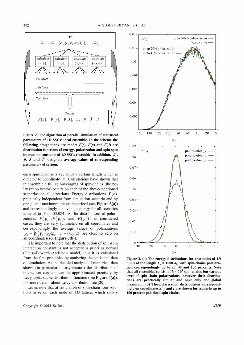
Figure 2. The algorithm of parallel simulation of statistical parameters of 1D SSCs’ ideal ensemble. In the scheme the following designations are made: F(ε), F(p) and F(J) are distribution functions of energy, polarization and spin-spin interaction constants of 1D SSCs ensemble. In addition, , p , J and 2J designate average values of corresponding parameters of system. each spin-chain is a vector of a certain length which is directed to coordinate x . Calculations have shown that in ensemble a full self-averaging of spin-chains (the po-larization vector) occurs on each of the above-mentioned scenarios on all directions. Energy distributions ( )F practically independent from simulation scenario and by one global maximum are characterized (see Figure 3(a)) and correspondingly the average energy for all scenarios is equal to 53.084 . As for distributions of polari-zations, , ,x yF p F p and zF p , in considered cases, they are very symmetric on all coordinates and correspondingly the average values of polarizations

= dp F p p p ; = { , , }x y z are close to zero on all coordinates(see Figure 3(b)).

It is important to note that the distribution of spin-spin interaction constant is not accepted a priori as normal (Gauss-Edwards-Anderson model), but it is calculated from the first principles by analyzing the statistical data of simulation. As the detailed analysis of numerical data shows (in particular its asymptotes) the distribution of interaction constant can be approximated precisely by Lévy alpha-stable distribution function (see Figure 4(a)). For more details about Le'vy distribution see [20].

Let us note that at simulation of spin-chain four solu-tions arise on each node of 1D lattice, which satisfy

(a)

(b)

Figure 3. (a) The energy distributions for ensembles of 1D SSCs of the length Lx = 1000 d0, with spin-chains polariza-tion correspondingly up to 20, 40 and 100 percents. Note that all ensembles consist of 5 × 104 spin-chains but various level of spin-chain polarizations, however their distribu-tions are practically similar and have only one global maximum; (b) The polarization distributions correspond-ingly on coordinates x, y and z are shown for scenario up to 100 percent polarized spin-chains.



493

(a)

(b)

Figure 4. (a) The distribution of spin-spin interaction con-stant essentially differs from Gauss-Edwards- Anderson distribution model and corresponds to Lev’y alpha-stable distributions class. The green curve is fitted by Cauchy function; (b) It is obvious from the graphic that for a wide range of parameter γ there is not any phase transition in the spin-glass system depending on the amplitude of an exter-nal field. It means that under the influence of an external field the system is reconstructed so, that the average energy of spin-chain practically is not being changed.

equations of stationary points (5). It is possible to think that it would lead to exponentially growth of number of solutions along with increase in number of nodes or length of spin-chain. However, such scenario of solutions branching does not occur due to accounting of additional conditions (6)-(7) and also (16) (see the numerical simu-lation for different initial parameters Figure 5).

At last it is important to recall that condition (16) plays an important role during the modeling. This condi-tion specifies the border of regions where interaction constants J are localized and thus the process of simula-tion is very effective (see Figure 6).

Figure 5. On the figure the process of solutions ν branching with increase in length of 1D spin-chains is shown. As one can see the number of solutions does not exceed 12 on each layer of branching for spin-chains of length Nx and till the end of the spin-chain it is independent from the initial an-gular configurations needed for the start of the simulation.

Figure 6. On the picture localization regions changes of the spin-spin interaction constants are shown, depending on the node sequence number of 1D lattice. Different colors cor-respond to different numerical experiments.



494

5. Statistical Properties of Ensemble in External Field

Using the obvious similarity between temperature T of usual statistical ensemble and the average energy coming on one spin 0 = xN we can define the partition function as follows:

1

0

d ;d; = exp ,

4 4

N xxH N g

Z g J

(19)

where J describes the set of spin-spin interaction con-stants in chain.

The integration in the expression (19) in above-mentioned model may start from the end of the chain (see [21]). When integrating over the solid angle d i we take the direction of the vector 0

1S hii i iJ p as a polar axis and it is easy to obtain the following expres-sion:

1

=0

22 0 01 1 1

0

sinh; = ,

1; , = 2 cos .

Nxi

i i

i ii ii i ii i i

GZ g J

G

G g J J p h J p h

(20) Assuming that the distribution of spin 1iS around

the field ih direction is isotropic, one can perform an integration over the angle i and after simple calcula-tions find:

1 π

0=0 0

1

0 1=0

sinh1, ; = sin d

2

1= ; , ,

Nxi

i ii i

Nx

i iii i

GZ g J

G

g Jb

(21)

where

0 1

01

0

012

0

; , = cosh cosh ,

1= ,

2= .

i ii i i

i ii i

i ii i

g J a a

a J p h

b J p h

Now using the expression (21) we can average the partition function by distribution ( )F J :

1

00 0 00

=0 ,

1, , ; = , ; ,

Nx

iJi i j J

Z g Z g J g Jb

(22) where

01 1 01 1. d dN N N NJ x x x xF J F J J J .

Like in the usual thermodynamics, Helmholtz free en-ergy for 1D SSC ensemble may be specified in the fol-lowing kind:

0 0 0 0, = ln , , < 0.Q g Z g (23)

Note that all thermodynamic properties of the statistical system in this case may be obtained by means derivation of the free energy by external field parameters g. After the derivation of the free energy by 0h we can find:

1

0

=00

, 1, = = 1 coth ,

Nx

x i ii

Q gq N y y

h

(24)

where

00 0 0 0

0

= , = , = cos ,

= , = 2π .

i N ix

i N xx

h h p h y k x

x id k N

As calculations show, the free energy derivation line-arly depends on parameter. The last result testifies the absence of a phase transition on this parameter (see Figure 4(b)). Thereby a logical question arises - are there phase transitions in considered system depending on other parameters?

To answer this question we will investigate the be-havior of the average value of polarization depending on parameter or the value of an external field.

Using the definition (8) we can calculate the polariza-tion distribution on coordinates ,F p , where

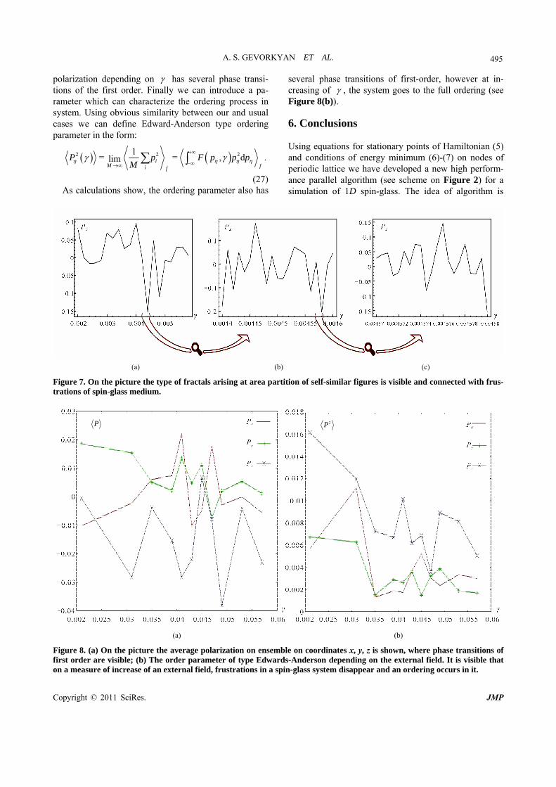
= , , .x y z As numerical simulation shows, distribu-tions of polarizations depending on parameter are strongly frustrated [22] and these frustrations do not dis-appear at regular dividing of computation region (see Figures 7(a), (b), (c)). Moreover, at each division a self-similar structure is conserved which testifies about its fractal character. The dimensionality of fractal struc-ture is calculated by simple formula:

= ln ln ,D n N (25)

where n is the number of partitions of the structure size, and N is the number of placing of the initial structure. The calculation particularly shows, that at value of

= 0.00425 dimensionality 1.2095xD . In a similar manner yD and zD can be calculated. It is obvious that at increasing all of them converge to 1.

At last we will pass to a question on average value of polarization. Namely, how to calculate it? Taking into account above-mentioned, it is obvious that the average value of polarization (magnetization) must be calculated by following formula:

1= = , dlim i

M fi f

P p F p p pM

(26)

where the slanting bracket .f

stands for averaging of expression by the fractal structure which itself represents an arithmetic mean. As follows from the Figure 8(a), after averaging on fractal structures the average value of



495

polarization depending on has several phase transi-tions of the first order. Finally we can introduce a pa-rameter which can characterize the ordering process in system. Using obvious similarity between our and usual cases we can define Edward-Anderson type ordering parameter in the form:

2 2 21= = , d .lim i

M fi f

P p F p p pM

(27) As calculations show, the ordering parameter also has

several phase transitions of first-order, however at in-creasing of , the system goes to the full ordering (see Figure 8(b)). 6. Conclusions Using equations for stationary points of Hamiltonian (5) and conditions of energy minimum (6)-(7) on nodes of periodic lattice we have developed a new high perform-ance parallel algorithm (see scheme on Figure 2) for a simulation of 1D spin-glass. The idea of algorithm is

(a) (b) (c)

Figure 7. On the picture the type of fractals arising at area partition of self-similar figures is visible and connected with frus-trations of spin-glass medium.

P 2P

(a) (b)

Figure 8. (a) On the picture the average polarization on ensemble on coordinates x, y, z is shown, where phase transitions of first order are visible; (b) The order parameter of type Edwards-Anderson depending on the external field. It is visible that on a measure of increase of an external field, frustrations in a spin-glass system disappear and an ordering occurs in it.



496 based on the construction of stable spin-chains of certain lengths. We have shown that the number of spin-chains (the simulation number) can be considered as a “timing” parameter as in case of dynamic system and the ergodic properties of system can be studied depending on this parameter. It is shown by numerical experiments that distribution functions of different parameters of the sys-tem after 2

xN simulations converge to the equilibrium values. In other words, system which consists of 2

xN number spin-chains satisfies Birkhoff's ergodicity condi-tions. We have shown that the distribution of spin-spin interaction constants can be found directly by way of calculations of classical Equations (5) and analysis of statistical data of simulation. It is theoretically shown (see inequality (16)) that at least for the 1D spin-glass problem the distribution of the spin-spin interaction con-stants can not be Gauss-Edwards-Anderson type. In par-ticular, the analysis of numerical data of simulation shows that they obey to Lévys alpha-stable distribution law. In other words, if we use the normal distribution in these problems, we make calculations ineffective, not to say doubtful.

As it is shown, the derivative of a free energy (24) does not have a phase transition depending on the pa-rameter of an external field’s energy (see Figure 4(b)). The last means that under the influence of an external field the essential changes of energy does not occur in the system. The last, however, does not mean that in the system a critical phenomena can not occur under the in-fluence of an external field related to other parameters. Only through numerical calculations we were able to show that in the system the phase transitions of first or-der occur under the influence of weak external field in the value of average polarization of spin-glass on all co-ordinates (see Figure 8(a)). As calculations show, the critical phenomena can be considerable even for weak fields. For example, they can lead to formation of a su-perlattice of a dielectric constant in the spin-glass’ me-dium which can have a wide applications for solutions of different applied problems.

Finally, it is important to note that the algorithm can be simply generalized for high dimensional cases and in particular for 3D case, which means that it will be a very needed instrument for numerical investigations of above- mentioned class of problems. 7. References [1] K. Binder and A. P. Young, “Spin Glasses: Experimental

Facts, Theoretical Concepts and Open Questions,” Re-views of Modern Physics, Vol. 58, No.4, 1986, pp. 801- 976. doi:10.1103/RevModPhys.58.801

[2] M. Mézard, G. Parisi and M. A. Virasoro, “Spin Glass

Theory and Beyond,” Vol. 9, World Scientific, Singapore, 1987.

[3] A. P. Young, “Spin Glasses and Random Fields,” World Scientific, Singapore, 1998.

[4] R. Fisch and A. B. Harris, “Spin-Glass Model in Con-tinuous Dimensionality,” Physical Review Letters, Vol. 47, No. 8, 1981, p.620. doi:10.1103/PhysRevLett.47.620

[5] C. Ancona-Torres, D. M. Silevitch, G. Aeppli and T. F. Rosenbaum, “Quantum and Classical Glass Transitions in LiHOxY1-xF4,” Physical Review Letters, Vol. 101, No. 5, 2008, pp. 057201.1-057201.4.

[6] A. Bovier, “Statistical Mechanics of Disordered Systems: A Mathematical Perspective,” Cambridge Series in Sta-tistical and Probabilistic Mathematics, No. 18, 2006, p 308.

[7] Y. Tu, J. Tersoff and G. Grinstein, “Properties of a Con-tinuous-Random-Network Model for Amorphous Sys-tems,” Physical Review Letters, Vol. 81, No. 22, 1998, pp. 4899-4902. doi:10.1103/PhysRevLett.81.4899

[8] K. V. R. Chary and G. Govil, “NMR in Biological Sys-tems: From Molecules to Human,” Springer, Vol. 6, 2008, p. 511.

[9] E. Baake, M. Baake and H. Wagner, “Ising Quantum Chain is an Equivalent to a Model of Biological Evolu-tion,” Physical Review Letters, Vol. 78, No. 3, 1997, pp. 559-562. doi:10.1103/PhysRevLett.78.559

[10] D. Sherrington and S. Kirkpatrick, “A Solvable Model of a Spin-Glass,” Physical Review Letters, Vol. 35, No. 26, 1975, pp. 1792-1796. doi:10.1103/PhysRevLett.35.1792

[11] B. Derrida, “Random-Energy Model: An Exactly Solv-able Model of Disordered Systems,” Physical Review B, Vol. 24, No. 5, 1981, pp. 2613-2626. doi:10.1103/PhysRevB.24.2613

[12] G. Parisi, “Infinite Number of Order Parameters for Spin-Glasses,” Physical Review Letters, Vol. 43, No. 23, 1979, pp. 1754-1756. doi:10.1103/PhysRevLett.43.1754

[13] A. J. Bray and M. A. Moore, “Replica-Symmetry Break-ing in Spin-Glass Theories,” Physical Review Letters, Vol.41, No. 15, 1978, pp. 1068-1072. doi:10.1103/PhysRevLett.41.1068

[14] J. F. Fernandez and D. Sherrington, “Randomly Located Spins with Oscillatory Interactions,” Physical Review B, Vol. 18, No. 11, 1978, pp. 6270-6274. doi:10.1103/PhysRevB.18.6270

[15] F. Benamira, J. P. Provost and G. J. Vallée, “Separable and Non-Separable Spin Glass Models,” Journal de Phy-sique, Vol. 46, No. 8, 1985, pp. 1269-1275. doi:10.1051/jphys:019850046080126900

[16] D. Grensing and R. Kühn, “On Classical Spin-Glass Models,” Journal de Physique, Vol. 48, No. 5, 1987, pp. 713-721. doi:10.1051/jphys:01987004805071300

[17] A. S. Gevorkyan, et al., “New Mathematical Conception and Computation Algorithm for Study of Quantum 3D Disordered Spin System under the Influence of External Field,” Transactions on Computational Science VII, 2010, pp. 132-153.



497

[18] S. F. Edwards and P. W. Anderson, “Theory of Spin Glasses,” Journal of Physics F, Vol. 5, 1975, pp. 965-974. doi:10.1088/0305-4608/5/5/017

[19] A. S. Gevorkyan, H. G. Abajyan and H. S. Sukiasyan, ArXiv: cond-mat.dis-nn 1010.1623v1.

[20] I. Ibragimov and Y. Linnik, “Independent and Stationary

Sequences of Random Variebles,” Mathematical Reviews, Vol. 48, 1971, pp. 1287-1730.

[21] C. J. Thompson, “Phase Transitions and Critical Phe-nomena,” Academic Press, Vol. 1, 1972, pp. 177-226.

[22] E. Bolthausen and A. Bovier, “Spin Glasses,” Springer, Vol. 163, No. 6, 2007, pp. 1900-2075.

A New Parallel Algorithm for Simulation of Spin-Glass ... · the following time-correspondences...

Documents

Transcript of A New Parallel Algorithm for Simulation of Spin-Glass ... · the following time-correspondences...