101-1

A New MPS Simulation Algorithm Based on Gibbs Sampling

Steven Lyster1, Clayton V. Deutsch1, and Thies Dose2

1Centre for Computational Geostatistics – Edmonton, Alberta

2RWE Dea Aktiengsellschaft – Hamburg, Germany

The major heterogeneity in most reservoirs and deposits is often characterized by facies or rock types. Petrophysical properties are modeled within each facies or rock type. Multiple-point geostatistical methods are being used increasingly to reproduce curvilinear geologic features. A number of multiple-point simulation methods have been put forward in the past; this paper proposes a novel implementation using a Gibbs sampler algorithm. This algorithm uses the concept of multiple-point events in an effort to account for high-order structure in the presence of arrangements of facies which are inconsistent with the statistics inferred from the training image.

Introduction

Multiple-point statistics (MPS) methods are used to model geologic phenomena in more realistic and robust ways than traditional geostatistics. Rather than considering linear estimates based on individual conditioning points, MPS use several points simultaneously to determine conditional probabilities. These higher-order relations more accurately describe complex features than the standard Gaussian model of spatial structure.

Several methods for reproducing MPS have been explored previously: the single normal equation (SNE) approach first proposed by Guardiano and Srivastava (1993) and further expanded by Strebelle and Journel (2000, 2001); simulated annealing (Deutsch, 1992; Lyster et al, 2004a); Gibbs sampling (Srivastava, 1992); a neural network iterative scheme (Caers and Journel, 1998; Caers, 2001); and integration of runs with indicator simulation for reproduction of higher-order relations in continuous data (Ortiz, 2003).

MPS methods have primarily focused on categorical indicators and modeling rock types; this is probably due to the relative ease with which training images may be created for geologic structures, as opposed to the dense sampling necessary to infer high-order moments for continuous data. Within the family of categorical methods, most use iterative approaches to reproduce MPS. This is likely because of the relative reduction in dimensionality of the statistics that must be calculated and stored when using a template in an iterative method, instead of having to characterize the many combinations of both points and facies needed for a sequential method.

The approach proposed in this paper is similar to several of the above-mentioned methods in that it is an iterative simulation algorithm meant to be used for modeling of geologic facies or rock types. While a Gibbs sampler method has been investigated before, a novel technique for determining the conditional probabilities will be presented. Several updating schemes to enforce proper univariate statistical reproduction and locally varying proportions will also be discussed. Two examples using complex training images and comparing two-point with MPS simulation results will be shown. A comparison of the proposed algorithm with several other MPS simulation methods will also be undertaken; the training image for this comparison is a three-dimensional model of a fluvial petroleum reservoir.

101-2

Gibbs Sampler

The Gibbs sampler is a statistical algorithm that was first proposed by Geman and Geman (1984); it is a special case of the Metropolis algorithm (Metropolis et al, 1953). It is a method used for drawing samples from complicated joint or marginal distributions, without requiring the density functions of the distributions (Casella and George, 1992). In the context of geological modeling, a sample from the joint distribution is a simulated realization. In a Gibbs sampler only the conditional distributions are required to sample from the joint distribution, which is why this approach is attractive as a MPS simulation method; all necessary conditional probabilities may be determined from a training image.

The basic idea of a Gibbs sampler is that of resampling individual variables conditional to others in the same sample space. Drawing new values conditional to all others, and repeating this process many times, results in an approximation of the joint (and marginal) distribution(s). For example, to determine the density function for f(X,Y,Z), one would start with an initial state (values) for X, Y, and Z and then sequentially draw values from the conditional distributions f(X|Y,Z), f(Y|X,Z), and f(Z|X,Y). When a number of conditional values have been drawn, the state of (X,Y,Z) approximates a sample from the joint distribution f(X,Y,Z). Repeating this process enough times allows the density (or histogram) of the joint distribution to be constructed empirically. In geostatistics generating many samples from the joint distribution is analogous to creating many simulated realizations.

The Gibbs sampler is a Markov chain Monte Carlo (MCMC) method (Gelfand and Smith, 1990), meaning that each new value drawn from a conditional distribution is assumed to be dependent only on the current state of the variables. While theoretically the new value should be dependent on all prior states, because the current state is dependent on the previous state and the previous dependent on the one before that; thus, using only the current state to determine the new value drawn accounts for all earlier states and therefore the theory may be simplified to ignore all past states and use only the current. This property is known as conditional independence, and allows the use of a MCMC method in a geoscience application to be greatly simplified.

An advantage of the Gibbs sampler workflow for geospatial modeling is that there is no strict specification for how the conditional distributions need to be determined. Previous use of the Gibbs sampler (Srivastava, 1992) focused primarily on using kriging and two-point statistics; a single normal equation using MPS was also explored briefly. Besides a MPS template, it would be possible to integrate any desired statistics into the conditionals, such as locally varying means, secondary data, and lower-order statistics to ensure their proper reproduction. The results of the simulation will be dependent on the selection of the conditional distribution chosen.

Estimation of Conditional Probabilities

To find the conditional probabilities of facies at a point, any desired method could be used. However, the quality of the resulting realizations will be determined by the conditional probabilities selected. For example, using only the univariate histogram as a conditional distribution would guarantee that the facies proportions are matched exactly, but would not give any structure in the results; using the variograms and kriging to determine conditional probabilities would reproduce the direct covariance structure but nothing more; adding the cross-variograms in a licit LMC would reproduce the relations between facies as well. The use of MPS should hopefully reproduce higher-order statistics in the end results.

101-3

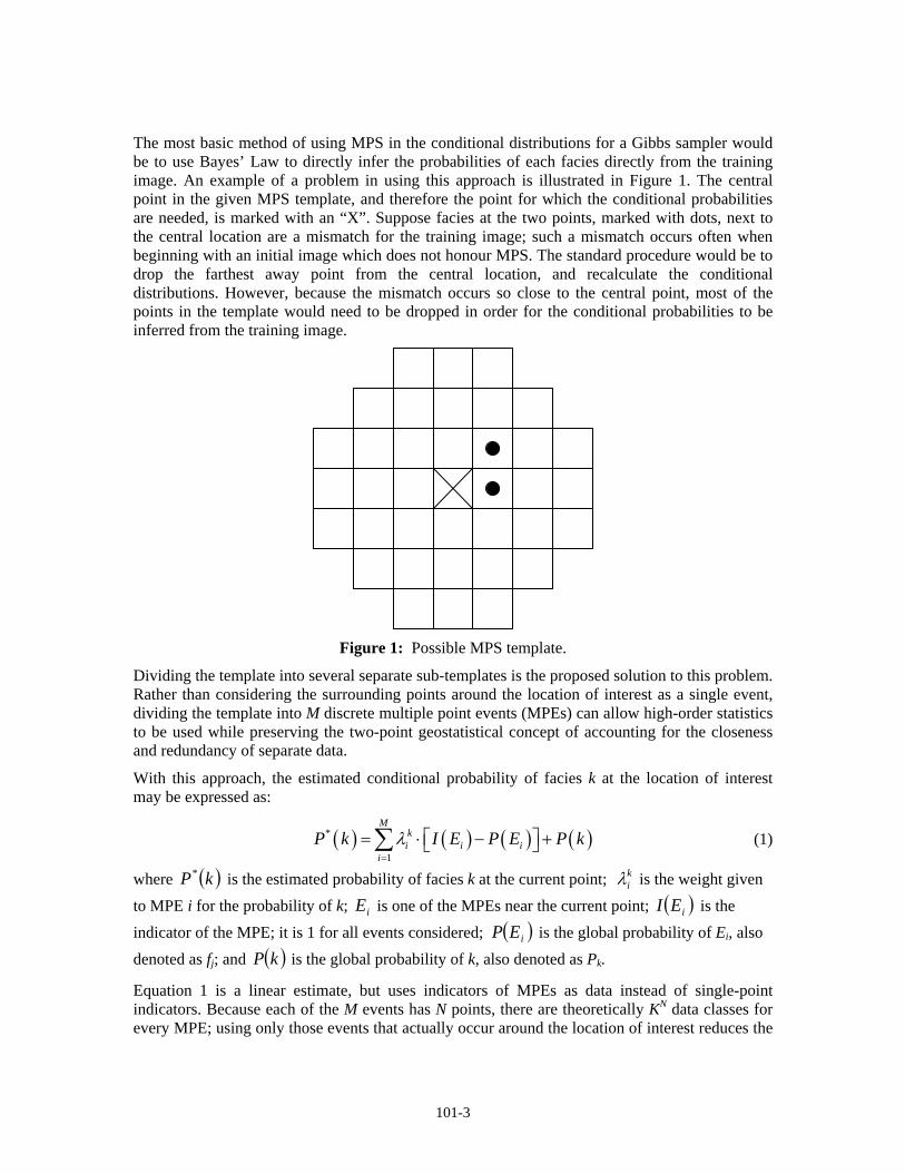
The most basic method of using MPS in the conditional distributions for a Gibbs sampler would be to use Bayes’ Law to directly infer the probabilities of each facies directly from the training image. An example of a problem in using this approach is illustrated in Figure 1. The central point in the given MPS template, and therefore the point for which the conditional probabilities are needed, is marked with an “X”. Suppose facies at the two points, marked with dots, next to the central location are a mismatch for the training image; such a mismatch occurs often when beginning with an initial image which does not honour MPS. The standard procedure would be to drop the farthest away point from the central location, and recalculate the conditional distributions. However, because the mismatch occurs so close to the central point, most of the points in the template would need to be dropped in order for the conditional probabilities to be inferred from the training image.

Figure 1: Possible MPS template.

Dividing the template into several separate sub-templates is the proposed solution to this problem. Rather than considering the surrounding points around the location of interest as a single event, dividing the template into M discrete multiple point events (MPEs) can allow high-order statistics to be used while preserving the two-point geostatistical concept of accounting for the closeness and redundancy of separate data.

With this approach, the estimated conditional probability of facies k at the location of interest may be expressed as:

( ) ( ) ( ) ( )*

1

Mki i i

iP k I E P E P kλ

=

⎡ ⎤= ⋅ − +⎣ ⎦∑ (1)

where ( )kP* is the estimated probability of facies k at the current point; kiλ is the weight given

to MPE i for the probability of k; iE is one of the MPEs near the current point; ( )iEI is the indicator of the MPE; it is 1 for all events considered; ( )iEP is the global probability of Ei, also denoted as fj; and ( )kP is the global probability of k, also denoted as Pk.

Equation 1 is a linear estimate, but uses indicators of MPEs as data instead of single-point indicators. Because each of the M events has N points, there are theoretically KN data classes for every MPE; using only those events that actually occur around the location of interest reduces the

101-4

size of the linear estimate from MKN terms to M. This reduction in dimensionality should not have a significant impact, as the weights for such a very large linear estimate would be relatively small and the global probabilities of MPEs also quite small; therefore, those MPEs whose indicators are 1 should have by far the greatest impact on the estimated conditional probabilities.

Minimizing the variance of the estimated conditional probabilities given in Equation 1 leads to:

( ) ( ) ( ) ( ) ( ) ( ) ( ) ( )

( ) ( ) ( ) ( ) ( ) ( ) ( ) ( )

( ) ( )

222

1 1

1 1 12

M Mk k

P i i i i i ii i

M M Mk k ki j i i j j i i i

i j i

ki i i

E I E P E I k P k E I E P E I k P k

E I E P E I E P E E I E P E I k P k

P E P E

σ λ λ

λ λ λ

λ

= =

= = =

⎧ ⎫ ⎡ ⎤⎡ ⎤ ⎧ ⎫⎪ ⎪⎡ ⎤ ⎡ ⎤ ⎡ ⎤ ⎡ ⎤= ⋅ − − − − ⋅ − − −⎨ ⎬ ⎨ ⎬⎢ ⎥⎢ ⎥⎣ ⎦ ⎣ ⎦ ⎣ ⎦ ⎣ ⎦⎣ ⎦ ⎩ ⎭⎣ ⎦⎪ ⎪⎩ ⎭⎧ ⎫ ⎧ ⎫⎡ ⎤⎡ ⎤ ⎡ ⎤ ⎡ ⎤= ⋅ ⋅ − ⋅ − − ⋅ ⋅ − ⋅ −⎨ ⎬ ⎨ ⎬⎣ ⎦ ⎣ ⎦ ⎣ ⎦⎣ ⎦ ⎩ ⎭⎩ ⎭

⎡− ⋅ −⎣

∑ ∑

∑∑ ∑

( ) ( )

( ) ( ) ( ) ( ) ( ) ( ) ( ) ( )

2

1

2

1 1 12

M

i

M M Mk k ki j i j i j i i i

i j i

P k P k

P E E P E P E P E k P E P k P k P kλ λ λ

=

= = =

⎡ ⎤⎤ ⎡ ⎤− −⎢ ⎥⎦ ⎣ ⎦⎣ ⎦

⎡ ⎤⎡ ⎤ ⎡ ⎤= ⋅ ⋅ ∩ − ⋅ − ⋅ ⋅ ∩ − ⋅ + −⎣ ⎦⎣ ⎦ ⎣ ⎦

∑

∑∑ ∑

(2)

To continue with the derivation it becomes necessary to define the covariance between MPEs:

{ } ( ) ( )[ ] ( ) ( )[ ]{ } ( ) ( ) ( )jijijjiiji EPEPEEPEPEIEPEIEEECov ⋅−∩=−⋅−=, (3)

Substituting Equation 3 into Equation 2,

{ } { } { }kVarkECovEECovM

ii

ki

M

i

M

jji

kj

kiP +⋅⋅−⋅⋅= ∑∑∑

== = 11 1

2 ,2, λλλσ (4)

And now taking the derivative and setting it equal to zero,

{ } { }kECovEECov i

M

jji

kjk

i

P ,2,21

2

⋅−⋅⋅=∂∂ ∑

=

λλσ

Mi ,,1…=

{ } { }kECovEECov i

M

jji

kj ,,

1=⋅∑

=

λ Mi ,,1…= (5)

Equation 5 is exactly the same as the standard simple kriging system of equations, with MPEs as data. Because training images are used in MPS all necessary covariances, even those involving complex MPEs, may be easily inferred.

To justify the use of the proposed approach utilizing MPEs, several checks may be made. Firstly, if each event considered consists of a single point then the estimate in Equation 1, the covariance in Equation 3, and the kriging system in Equation 5 all become the standard equations used in traditional two-point geostatistics. This suggests that the theory behind MPEs is sound, and is a more general form of traditional indicator geostatistics.

The second check for the validity of the proposed method is to use only a single event of N points. In this case, solving for the optimal weight in Equation 5 yields

{ }{ }

( ) ( ) ( )( ) ( )[ ]11

11

11

11 1,

,EPEP

kPEPkEPEECovkECovk

−⋅⋅−∩

==λ (6)

Substituting this result into Equation 1, the estimated conditional probabilities are then

101-5

( ) ( ) ( ) ( )( ) ( )[ ] ( ) ( )[ ] ( )kPEPEI

EPEPkPEPkEPkP +−⋅

−⋅⋅−∩

= 1111

11*

1

And since the indicator of the event occurring is always 1, this simplifies to

( ) ( )( )

( ) ( )( ) ( ) ( )1

1

1

1

1* | EkPkPEP

kPEPEP

kEPkP =+⋅

−∩

= (7)

Equation 7 is Bayes’ Law, which is exactly the result that should be expected when using a single event as data for determining conditional probabilities.

Modifications to Conditional Probabilities

In addition to the MPE approach for estimating the conditional probabilities, other factors may be considered as required. As mentioned previously there are no strict requirements for the conditional probabilities used in a Gibbs sampler; there is only the practical result that better selection of the conditional distributions will yield more accurate estimates of the joint distribution and hence higher-quality realizations.

Keeping with this idea, adjustments to the estimated conditional probabilities may be made to help ensure the global target statistics are honoured. The first modification is to help reproduce the global univariate proportions, which are often considered very important. To guide the global proportions towards those desired, a servosystem is employed in the new algorithm (Strebelle and Journel, 2001). The servosystem modifies the estimated conditional probabilities as follows:

( ) ( ) ( ) ( )kPkPkPkP C−+=′ * (8)

where ( )kP′ is the modified conditional probability of facies k; ( )kP* is the estimated probability of facies k found with Equation 1; ( )kP is the global probability of facies k; and

( )kPC is the proportion of facies k in the current realization field

This modification leads to the facies which are underrepresented being gradually introduced more often and those which occur too often being subtly decreased. While the servosystem in Equation 8 is unlikely to drastically affect the conditional probabilities, it will prevent the univariate proportions from deviating too far from those desired.

In addition to the servosystem modification, an additional updating scheme is needed to honour locally varying proportions of facies. While local proportions could be inserted directly into Equation 8, the decision was made to use a Bayesian updating scheme (Deutsch, 2002) instead. This is an arbitrary decision and could be easily modified in the future. The Bayesian updating scheme for local proportions is as follows:

( ) ( ) ( )( )kP

kPkPkPL

×′=′′ (9)

where ( )kP ′′ is the updated conditional probability of facies k; and ( )kP L is the local probability of facies k.

101-6

Using Bayesian updating as in Equation 9 should have a greater impact on the conditional probabilities of facies with low global proportions than an additive servosystem. For example, if a facies has a global Pk = 0.1 and the local Pk = 0.2, an additive modification would add 0.1 to the estimated conditional probability; this may not be significant enough to overcome the global proportion term in Equation 1. Multiplying as in Equation 9 would double the estimated probability for this facies, which should have a greater effect.

Alternatively to the updating methods suggested here, a purely multiplicative approach could be used; this would result in the estimated conditional probabilities being multiplied by the local probabilities over the current realization proportions. This method was found to not be strict enough in matching the desired global proportions; as a facies is eroded away from the realization its probabilities become correspondingly lower, and multiplying a very low probability by some factor still results in a low probability. A purely additive approach was also explored, but was found to not honour the local means for those facies which have low global proportions. The proposed method is suggested as a compromise between the two alternatives.

Proposed Algorithm

Using the concepts discussed above, the proposed workflow for the new MPS simulation method is as follows:

1. Scan the training image and calculate all of the necessary statistics. Selection of the training image will not be discussed here. The number of MPEs to be used, M, and the points per event, N, must be selected carefully. Using more events will account for more of the surrounding information, but will also slow the algorithm down and put less weight on those events which are truly important. Too many points in each event will result in the statistics not being well enough informed from the training image; too few will not fully characterize complex features. Experimentation with the method has typically yielded the best results with M ranging from 4 to 12 and N of 4 to 8. The actual values used depend on the size and complexity of the training image, the number of facies being simulated, and the desired size and number of realizations.

2. Read in the initial image. The image itself should honour some of the desired features or statistics, such as the variogram; this speeds up the algorithm significantly and also improves the final results. If a random image is used there is likely to be very little useful information contained in the MPEs at each location, and therefore convergence to a sample from the joint distribution (ie, a realization) will be quite slow.

3. Develop a random path, spiraling away from the conditioning data. The data locations will not be visited, and therefore the data will be explicitly honoured. Spiraling away from the data should aid in the reproduction of conditioning information without discontinuities.

4. Follow the path, drawing new values. Estimate the conditional probabilities with Equation 1 and update with Equations 8 and 9. Draw a new facies value at each location from the updated conditional distribution. This is the Gibbs sampler part of the algorithm.

Drawing random values at every location has been found to often leave random noise and discontinuities in the resulting realizations, even though the overall structure is reproduced. Therefore, a version of maximum a-posteriori selection (MAPS) (Deutsch, 1998) has been implemented in the final loop of each realization to “clean up” the image.

101-7

MPS are still used to determine the conditional probabilities, however. The only modification to the estimation of the conditional distribution is the omission of the global mean values P(k) in Equation 1; working only with residuals, the updating is performed with Equations 8 and 9, then the facies with the maximum probability is selected. This results in the image being cleaned quite well without discarding many of the MPS honoured.

5. Finish the realization. After some number of loops over all locations (including the final MAPS loop), write out the results and repeat from step 2 for as many realizations as are desired. The number of loops is also a modeling choice which must be made for each individual case.

Example 1 – Channel Training Image, Two Facies

Shown at the top of Figure 2 is a two-dimensional training image with two facies: channel and non-channel. The image is 256 pixels square for a total of 65,536 cells. The channel structures seen in the training image have sinuosity and curvilinearity that is not possible to capture using two-point statistics. In the lower left of Figure 2 are two realizations created using sequential indicator simulation with the covariance calculated directly from the training image. While some of the general shape of the features is reproduced, such as the long east-west continuity and diagonal connectivity, in general there is very little reproduction of actual channels and potential flow paths are not seen in the realizations.

The lower right of Figure 2 shows two realizations produced with the proposed Gibbs sampler algorithm. Ten MPEs of six points each were used for determining the conditional probabilities; the two-point simulations shown on the left were used as initial images; and ten loops were performed including a single MAPS cleaning loop at the end. Simulating ten realizations took 8:13 using these parameters, including calculation of all relevant statistics. The computer used was a dual processor 3.2GHz PC with 3GB of RAM. Comparing these realizations to the SIS results, it is clear that the MPS enforce significantly more structure than two-point relations. Curvilinear bodies, long-range connectivity, and sinuosity in the channels are all evident.

In the current implementation of the method, conditional probabilities cannot be determined for the facies values at the very edge of the grid. For now this problem is simply being ignored, and the initial values at the boundary of the realization are left in place unchanged; in Figure 2 this may be seen as edge effects. This decision does not appear to have had too significant of an impact on the results in the rest of the grid, but a better method for dealing with edge effects is desirable.

Example 2 – Complex Training Image, Five Facies

A complex training image with five facies and very complex relations between the different codes is shown at the top of Figure 3. The image is 200 pixels by 100 pixels, a total of 20,000 cells. The lower left of Figure 3 shows three realizations which were produced using all relevant two-point statistics derived directly from the training image, including all direct and cross covariances. While some of the structure was properly reproduced (in particular the green diagonal banding), and many of the relations between facies were honoured (blue/red are inside/on top of light blue), the realizations look very little like the training image.

101-8

Using the proposed Gibbs sampler, the realizations look much more like the training image; three realizations are shown in the lower right of Figure 3. Ten realizations were constructed by using ten MPEs of three points each; twelve loops were performed, with the final one using the MAPS cleaning; and the two-point realizations in Figure 3 were used as initial images. Smaller MPEs were used than for the first example because, with a smaller training image and five different facies, there was less information from which to infer even higher-order MPS. Simulating the ten realizations took 2:03 on the same machine as that used for the first example. The elliptical bodies are much more clearly reproduced by MPS than two-point statistics, and the relations with the red and blue facies may be seen more clearly.

As seen previously, there are edge effects in the realizations in Figure 3. These artifacts once again appear to have little effect on the rest of the realization results. Considering the speed of the algorithm, it may be reasonable to consider simulating a larger grid than is needed and trimming the border.

Comparison with Other Simulation Methods

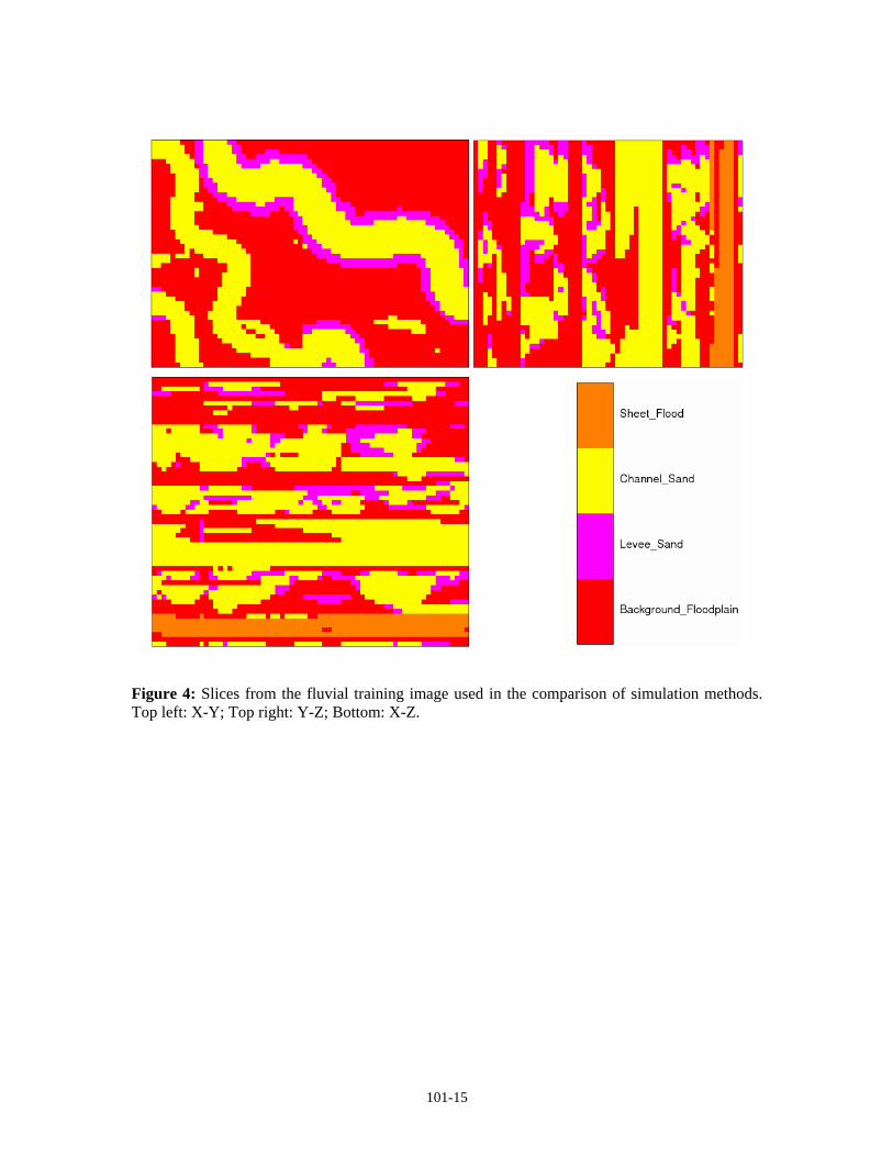
To analyze the potential of the proposed algorithm, a brief comparison study was performed. A complex three-dimensional training image with fluvial structures was used for the study; slices taken from this image are shown in Figure 4. The training image contains four facies: background floodplain (indicator code 0), levee sand (code 2), channel sand (code 4), and sheet flood sand (code 5). The image is 67 x 48 x 57 blocks in size, for a total of 183,312 blocks.

Six different simulation methods were considered in this study:

1. Full indicator cosimulation, with all covariances and cross covariances calculated directly from the training image. The program TISIS was used for this method (Lyster and Deutsch, 2006).

2. Single normal equation simulation using MPS; the SNESIM program was used (Strebelle and Journel, 2000).

3. Simulated annealing using 2x2x2 histograms of MPS as an objective function. This method used the MPASIM program (Lyster et al, 2004b).

4. Simulated annealing, post-processing the results of traditional two-point simulation. Again, the MPASIM program was used.

5. A “greedy” variant of simulated annealing, with the temperature set to zero; this case also used MPASIM.

6. Simulation using the proposed Gibbs sampler algorithm, using MPEs to determine conditional probabilities. A new program, MPESIM, was written for this purpose. Four MPEs of five points each were used for the simulation.

Ten realizations were created using each of the six methods listed above. The criteria used for the comparison were: time required for simulation, visual “goodness” of the realizations, reproduction of the target facies proportions in the training image, indicator variogram reproduction, error in the simulated MPS histograms, and distributions of multiple-point runs (Boisvert et al, 2006).

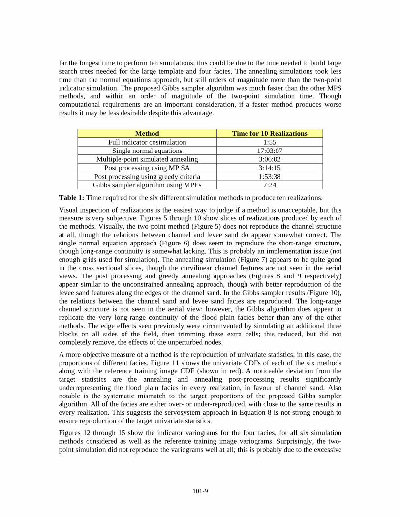
Table 1 gives a summary of the computational time required for each of the algorithms. As expected, the two-point method was the fastest. The single normal equation simulation took by

101-9

far the longest time to perform ten simulations; this could be due to the time needed to build large search trees needed for the large template and four facies. The annealing simulations took less time than the normal equations approach, but still orders of magnitude more than the two-point indicator simulation. The proposed Gibbs sampler algorithm was much faster than the other MPS methods, and within an order of magnitude of the two-point simulation time. Though computational requirements are an important consideration, if a faster method produces worse results it may be less desirable despite this advantage.

Method Time for 10 Realizations

Full indicator cosimulation 1:55 Single normal equations 17:03:07

Multiple-point simulated annealing 3:06:02 Post processing using MP SA 3:14:15

Post processing using greedy criteria 1:53:38 Gibbs sampler algorithm using MPEs 7:24

Table 1: Time required for the six different simulation methods to produce ten realizations.

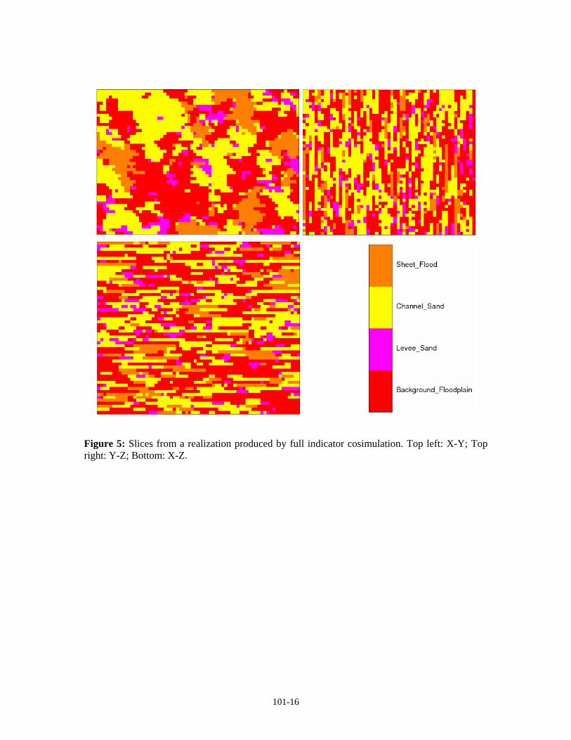
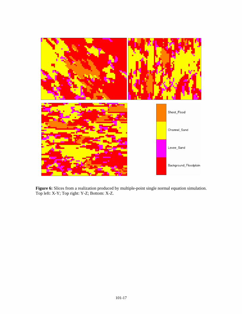
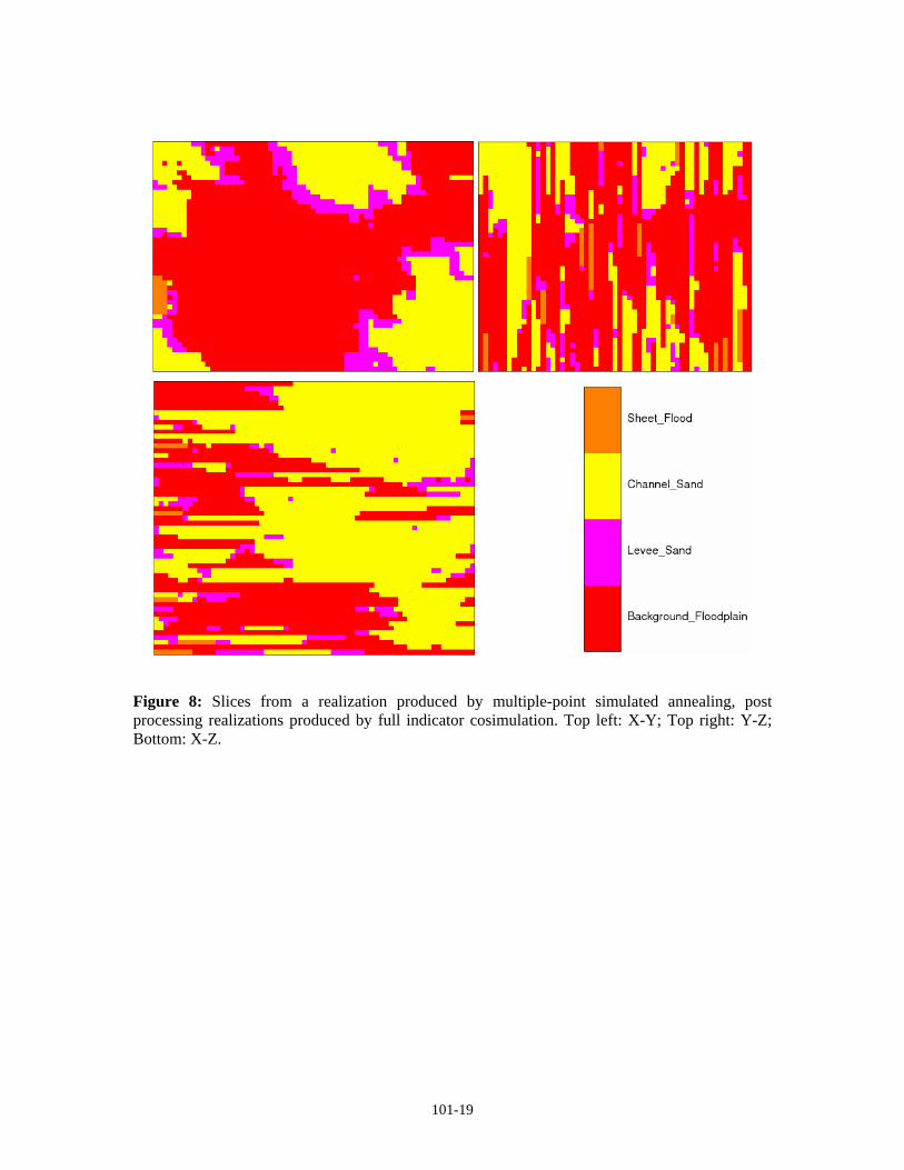
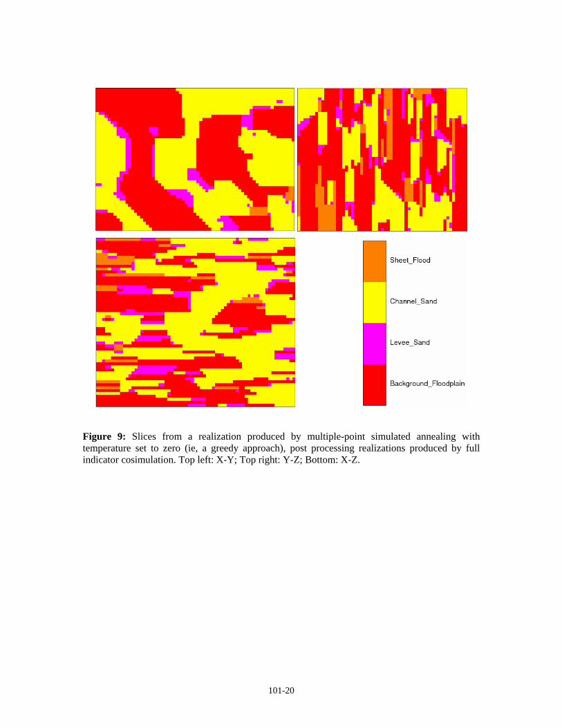
Visual inspection of realizations is the easiest way to judge if a method is unacceptable, but this measure is very subjective. Figures 5 through 10 show slices of realizations produced by each of the methods. Visually, the two-point method (Figure 5) does not reproduce the channel structure at all, though the relations between channel and levee sand do appear somewhat correct. The single normal equation approach (Figure 6) does seem to reproduce the short-range structure, though long-range continuity is somewhat lacking. This is probably an implementation issue (not enough grids used for simulation). The annealing simulation (Figure 7) appears to be quite good in the cross sectional slices, though the curvilinear channel features are not seen in the aerial views. The post processing and greedy annealing approaches (Figures 8 and 9 respectively) appear similar to the unconstrained annealing approach, though with better reproduction of the levee sand features along the edges of the channel sand. In the Gibbs sampler results (Figure 10), the relations between the channel sand and levee sand facies are reproduced. The long-range channel structure is not seen in the aerial view; however, the Gibbs algorithm does appear to replicate the very long-range continuity of the flood plain facies better than any of the other methods. The edge effects seen previously were circumvented by simulating an additional three blocks on all sides of the field, then trimming these extra cells; this reduced, but did not completely remove, the effects of the unperturbed nodes.

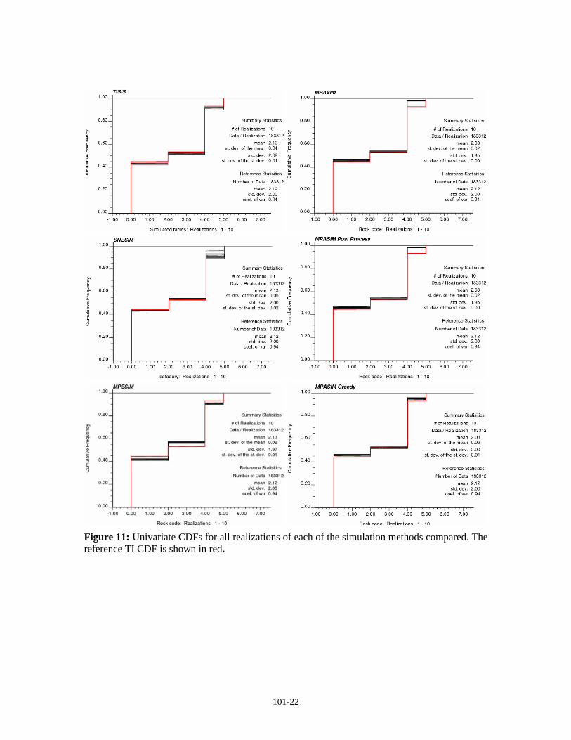
A more objective measure of a method is the reproduction of univariate statistics; in this case, the proportions of different facies. Figure 11 shows the univariate CDFs of each of the six methods along with the reference training image CDF (shown in red). A noticeable deviation from the target statistics are the annealing and annealing post-processing results significantly underrepresenting the flood plain facies in every realization, in favour of channel sand. Also notable is the systematic mismatch to the target proportions of the proposed Gibbs sampler algorithm. All of the facies are either over- or under-reproduced, with close to the same results in every realization. This suggests the servosystem approach in Equation 8 is not strong enough to ensure reproduction of the target univariate statistics.

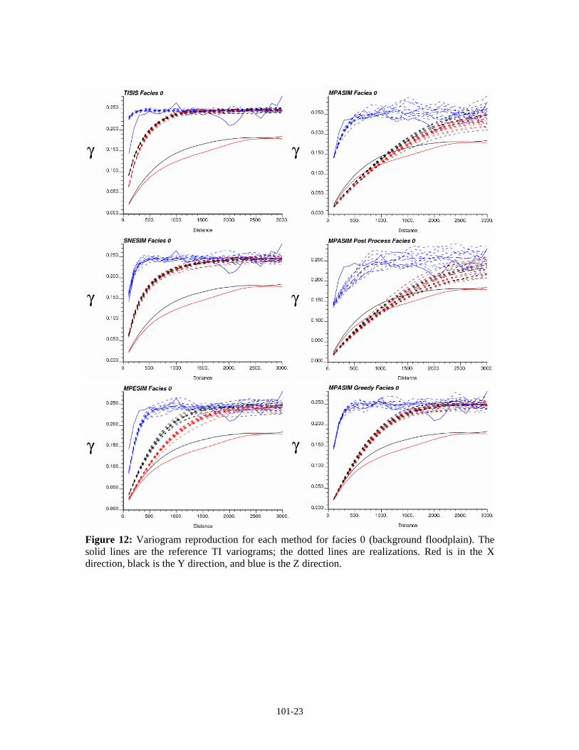
Figures 12 through 15 show the indicator variograms for the four facies, for all six simulation methods considered as well as the reference training image variograms. Surprisingly, the two-point simulation did not reproduce the variograms well at all; this is probably due to the excessive

101-10

randomness caused by large kriging matrices. The different flavours of annealing appear to best match the target variograms, which is surprising considering the small template used for the objective function. The very long-range horizontal continuity of the sheet flood facies was not reproduced by most of the methods; only the annealing and annealing post-processing methods came close to matching the variograms, and both of those methods were significantly skewed in the reproduction of the univariate proportion of the sheet flood. The proposed Gibbs sampler reproduced the structures of each variogram (with the exception of the sheet flood), but the sills are wrong due to the bias in the univariate proportions which was mentioned above.

As the simulation methods being compared utilize MPS (with one exception), comparisons using multiple-point statistics are desirable. The MPS histograms, using 2x2x2 statistics, were compared to those calculated from the training image; the distributions of runs were also calculated and compared. The average error (deviation from reference) for the histograms and runs for each of the simulation methods is shown in Table 2, along with the rankings of each method.

As should be expected, the two-point simulation performed the worst by far when measured by MPS criteria. The single normal equation algorithm performed better in runs than in the histogram measure, and was middle of the pack overall. The annealing methods performed very well, particularly in the histogram measure; however, the MPS histogram could be biased towards the annealing because a 2x2x2 statistic was used for both the objective function and the histogram error calculation. The proposed Gibbs sampler method lagged somewhat behind in both MPS measures, though the results are not bad enough to discourage further development of the algorithm.

Method MPH Error Rank Runs Error Rank

Full indicator cosimulation 0.990 6 0.563 6 Single normal equations 0.586 5 0.169 3

Multiple-point simulated annealing 0.256 3 0.120 2 Post processing using MP SA 0.256 2 0.267 4

Post processing using greedy criteria 0.247 1 0.068 1 Gibbs sampler algorithm using MPEs 0.453 4 0.333 5

Table 2: Comparisons of multiple-point statistics. Average deviations of multiple-point histograms and runs distributions from the training image are shown, as well as rankings of the different methods.

Comparing the MPE Gibbs sampler methodology to other facies simulation techniques, there is certainly room for improvement. The proposed method did not produce the best results by any objective measure. However, given the great savings in time required for performing the simulation, future modifications to the algorithm could make it a very attractive possibility.

Conclusions

As a MPS simulation method, the proposed Gibbs sampler algorithm shows promise. Further refinement is needed to properly reproduce long-range features, to eliminate the edge effects, and to ensure conditioning data are honoured. Better reproduction of the desired MPS is also a goal, though this would likely be a side effect of the other improvements mentioned.

101-11

Long-range features may be introduced in the initial images, rather than in the algorithm itself. In general for iterative algorithms, better initial images will lead to better results. The edge effects could simply be trimmed, the border of the realizations could use a different method for selection of conditional probabilities, or the grid could be wrapped. All of these possibilities have their own positive and negative points.

Honouring conditioning data is the most important implementation aspect that needs to be developed. The major weakness of many iterative methods is that hard data are explicitly honoured, but with a discontinuity. This problem can easily present itself in the proposed Gibbs sampler. Several steps may be taken to try and prevent this: ensure the initial images honour the conditioning data, use locally varying proportions of facies to reduce the likelihood of sudden discontinuities, or modify the conditional probabilities to explicitly account for nearby hard data.

Overall improvement to the technique could be accomplished through greater sophistication. Hierarchical simulation of facies, integration of lower-order (but longer-range) statistics to the conditional probabilities, and other modifications are all possible because of the great speed of the algorithm; there is the possibility for improvements to be made, even if simulation proceeds slower because of it.

Developments of these aspects, as well as other implementation issues, will need to be further researched. Any method needs to be quite robust before it can be accepted and used in quantification of uncertainty. The advantages of MPS over traditional two-point methods are offset by the extent to which kriging-based algorithms have been developed. Having a diverse range of techniques which utilize MPS is beneficial to the field as each method may have its own area in which the algorithm works best. Development of each idea will progress over time, and as problems are solved for one method the same solution may be applicable to others and the robustness of MPS will be increased.

References

Boisvert, J.B., Pyrcz, M.J., and Deutsch, C.V. (2006) Choosing Training Images and Checking Realizations with Multiple Point Statistics. Centre for Computational Geostatistics, No. 8, awaiting publication.

Caers, J. (2001) Geostatistical Reservoir Modelling Using Statistical Pattern Recognition. Journal of Petroleum Science and Engineering, Vol. 29, No. 3, May 2001, pp 177-188.

Caers, J. and Journel, A.G. (1998) Stochastic Reservoir Simulation Using Neural Networks Trained on Outcrop Data. SPE Annual Technical Conference and Exhibition, New Orleans, Oct. 1998, pp 321-336. SPE #49026.

Casella, G. and George, E.I. (1992) Explaining the Gibbs Sampler. The American Statistician, Vol. 46, No. 3, Aug. 1992, pp 167-174.

Deutsch, C.V. (1992) Annealing Techniques Applied to Reservoir Modeling and the Integration of Geological and Engineering (Well Test) Data. Ph.D. Thesis, Stanford University, 304 p.

Deutsch, C.V. (1998) Cleaning Categorical Variable (Lithofacies) Realizations With Maximum A-Posteriori Selection. Computers & Geosciences, Vol. 24, No. 6, pp 551-562.

Deutsch, C.V. (2002) Geostatistical Reservoir Modeling. Oxford University Press, New York, 376 p.

101-12

Gelfand, A.E. and Smith, A.F.M. (1990) Sampling-Based Approached to Calculating Marginal Densities. Journal of the American Statistical Association, Vol. 85, No. 410, June 1990, pp 398-409.

Geman, S. and Geman, D. (1984) Stochastic Relaxation, Gibbs Distributions, and the Bayesian Restoration of Images. IEEE Transactions on Pattern Analysis and Machine Intelligence, No. 6, Nov. 1984, pp 721-741.

Guardiano, F.B. and Srivastava, R.M. (1993) Multivariate Geostatistics: Beyond Bivariate Moments. Soares, A., Editor, Geostatistics Troia ’92, Vol. 1, pp 133-144.

Lyster, S., Leuangthong, O., and Deutsch, C.V. (2004a) Simulated Annealing Post Processing for Multiple Point Statistical Reproduction. Centre for Computational Geostatistics, No. 6, 15 p.

Lyster, S., Ortiz, J.M, and Deutsch, C.V. (2004b) MPASIM: A Multiple Point Annealing Simulation Program. Centre for Computational Geostatistics, No. 6, 18 p.

Lyster, S. and Deutsch, C.V. (2006) TISIS: A Program to Perform Full Indicator Cosimulation Using a Training Image. Centre for Computational Geostatistics, No. 8, awaiting publication.

Metropolis, N., Rosenbluth, A.W., Rosenbluth, M.N., Teller, A.H., and Teller, E. (1953) Equations of State Calculations by Fast Computing Machines. Journal of Chemical Physics, Vol. 21, No. 6, pp 1087-1091.

Ortiz, J.M. (2003) Characterization of High Order Correlation for Enhanced Indicator Simulation. Ph.D. Thesis, University of Alberta, 255 p.

Srivastava, M. (1992) Iterative Methods for Spatial Simulation. Stanford Center for Reservoir Forecasting, No. 5, 24 p.

Strebelle, S.B. and Journel, A.G. (2000) Sequential Simulation Drawing Structures From Training Images. Kleingeld, W.J. and Krige, D.G., Editors, 6th International Geostatistics Congress, 12 p.

Strebelle, S.B. and Journel, A.G. (2001) Reservoir Modeling Using Multiple-Point Statistics. SPE Annual Technical Conference and Exhibition, New Orleans, Oct. 2001, 11 p. SPE #71324.

101-13

Figure 2: Top: TI with two facies and channel features. Left: Realizations produced using two-point statistics. Right: Realizations using the proposed Gibbs sampler algorithm.

101-14

Figure 3: Top: Complex TI with five facies. Left: Realizations using only covariances and cross-covariances. Right: Realizations using the proposed Gibbs sampler algorithm.

101-15

Figure 4: Slices from the fluvial training image used in the comparison of simulation methods. Top left: X-Y; Top right: Y-Z; Bottom: X-Z.

101-16

Figure 5: Slices from a realization produced by full indicator cosimulation. Top left: X-Y; Top right: Y-Z; Bottom: X-Z.

101-17

Figure 6: Slices from a realization produced by multiple-point single normal equation simulation. Top left: X-Y; Top right: Y-Z; Bottom: X-Z.

101-18

Figure 7: Slices from a realization produced by multiple-point simulated annealing. Top left: X-Y; Top right: Y-Z; Bottom: X-Z.

101-19

Figure 8: Slices from a realization produced by multiple-point simulated annealing, post processing realizations produced by full indicator cosimulation. Top left: X-Y; Top right: Y-Z; Bottom: X-Z.

101-20

Figure 9: Slices from a realization produced by multiple-point simulated annealing with temperature set to zero (ie, a greedy approach), post processing realizations produced by full indicator cosimulation. Top left: X-Y; Top right: Y-Z; Bottom: X-Z.

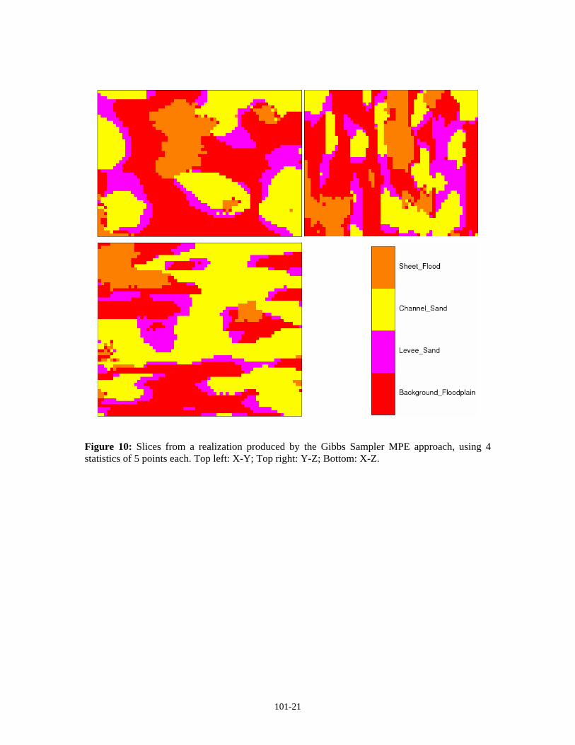
101-21

Figure 10: Slices from a realization produced by the Gibbs Sampler MPE approach, using 4 statistics of 5 points each. Top left: X-Y; Top right: Y-Z; Bottom: X-Z.

101-22

Figure 11: Univariate CDFs for all realizations of each of the simulation methods compared. The reference TI CDF is shown in red.

101-23

Figure 12: Variogram reproduction for each method for facies 0 (background floodplain). The solid lines are the reference TI variograms; the dotted lines are realizations. Red is in the X direction, black is the Y direction, and blue is the Z direction.

101-24

Figure 13: Variogram reproduction for each method for facies 2 (levee sand). The solid lines are the reference TI variograms; the dotted lines are realizations. Red is in the X direction, black is the Y direction, and blue is the Z direction.

101-25

Figure 14: Variogram reproduction for each method for facies 4 (channel sand). The solid lines are the reference TI variograms; the dotted lines are realizations. Red is in the X direction, black is the Y direction, and blue is the Z direction.

101-26

Figure 15: Variogram reproduction for each method for facies 5 (sheet flood). The solid lines are the reference TI variograms; the dotted lines are realizations. Red is in the X direction, black is the Y direction, and blue is the Z direction.