A New Model for Predicting Policy Choices

1

Conflict Management and Peace Science © The Author(s). 2010. Reprints and permissions:

http://www.sagepub.co.uk/journalsPermissions.nav [DOI: 10.1177/0738894210388127]

Vol 28(1): 1–21

A New Model for Predicting Policy ChoicesPreliminary Tests*

BRuCe BuenO De MeSquITAWilf Family Department of Politics, New York University

A new forecasting model, solved for Bayesian Perfect equilibria, is introduced. It, along with several alternative models, is tested on data from the european union. The new model, which allows for contingent forecasts and for generating confidence intervals around predictions, outperforms competing models in most tests despite the absence of variance on a critical variable in all but nine cases. The more proximate the political setting of the issues is to the new model’s underlying theory of competitive and potentially coercive politics, the better the new model does relative to other models tested in the european union context.

KeYWORDS: Bayesian updating; forecasting; game theory; prediction; policy engineering; policy analysis

The urge to predict future behavior has long been an interest of humankind. Whether by studying sheep entrails, star gazing, palm reading, or consulting oracles, people have wanted to find the means to discover the future. From early times, mathematicians have offered an alternative to divination, seers, and prophesy. They used logic, for example, to describe the area of any triangle, past, present or future or to discern the limits of number series, again whether in the present, the past or the future. Beginning more or less in the 17th century, the urge to predict pushed deductive theorists such as Hobbes and experimentalists such as Boyle to attempt to discover governing laws for physical phenomena, laws that could be used to predict future states of the world just as well as past states (Shapin and Shaffer, 1989). Isaac Newton propelled this form of science forward probably more than anyone, identi-fying laws (or nearly laws) governing motion—and the means through calculus to

* I am most grateful to Professors Robert Thomson and Frans Stokman for providing the data for this study as well as for their comments on earlier versions of the model tested here. I am also grateful to Christopher Butler, Charles Caldwell, Gene Downum, Robert Franzese, Nils Peter Gleditsch, Adam Meirowitz, Aron Patrick, Gerald Schneider, Allan Stam, and Rene Torenvlied for their most helpful comments and insights into earlier ver-sions of this model or this article. I also want to thank the students in my course, Solving Foreign Crises, who in the springs of 2008 and 2009 tested my new model for their course projects. I benefited greatly from their comments and suggestions.

Conflict Management and Peace Science 28(1)

2

measure change—that could be used to project the location of heavenly bodies into the distant future. Indeed, Newton’s logic was used in the 19th century to discover Neptune purely from mathematical logic (Sobel, 2006).

Today the urge to predict through science has motivated the development of numerous tools that rely on logic and evidence to anticipate outcomes of human activity into the future. These tools include such methods as evolutionary theory, game theory, computational models, classical statistics and probability theory, Bayesian estimation techniques, and many other modeling strategies. These have all proven their value through countless applications.

Here I introduce a new applied game theory model in an effort to contribute to progress on estimating future states of the world, especially with regard to fundamental problems in national security and in business. The emphasis in this study is on the empirical so I will briefly summarize the model’s construction and then turn to its empirical evaluation.

This article proceeds as follows. In the first section I summarize the objectives behind the models I propose. The next section briefly describes the structure of my old, so-called expected utility model before introducing the new model I am proposing. I also review the basics for estimating the variables in the new model and explain how they differ from the definition and estimation methods for the variables in my earlier model. The next section describes the data and structure of tests used to evaluate the two models, plus other predictive approaches, and in the subsequent section I report the findings. I conclude with a discussion of work to be done.

Modeling ObjectivesThe purpose behind the models described here is to predict the process and outcome leading to the resolution of complex negotiations or potentially coercive situations, including the possibility that they end with agreement, breakdown, or even the use of force. Predictive accuracy is an essential step toward political engineering, the ultimate application of such tools.

The modeling here is intended to be sufficiently generic that it can be applied to any situation involving the possibility of negotiation in the shadow of the threat (or the realization of the use) of coercion whether in the international arena, the domestic political arena, or in business or social interactions. It is not expected to be a reliable tool for predicting outcomes dictated purely by market forces in which no players or small group of players can move the market themselves or in which coercive threats have no role. It also is less likely to be effective in situations involving sufficient repeated play (as distinct from iterated play) among the same actors such that cooperative side deals, such as logrolls or vote trading, shape outcomes. As we will see, the tests performed here are mostly on just such data, making them especially demanding for both my new and old models.

Because of my purpose, the model must be capable of handling any number of players, specify their available actions, and have the flexibility to provide reliable real-time, short-term and long-term assessments of trends, tactics, and beliefs held by the stakeholders. What is more, because in the real world, unlike the pure theorist’s world, we cannot say in advance that a game will be played once; that it will iterate—with payoffs changing in response to earlier rounds of interaction—a

Bueno de Mesquita: Predicting Policy Choices

3

known fixed number of times; or that it will recur with fixed or variable payoffs an infinite number of times. The model must provide guidance as to when the game is predicted to end, as well as how it is predicted to end. And this, in turn, means that it is necessary to adopt some arbitrary heuristic rules designed to govern some key computational choices. These heuristic rules are combined with the axioms of game theory to capture strategic interaction. The chosen heuristic rules, of course, can be varied by others to determine their impact on outcomes without endangering the core strategic conceptual framework in which they are embedded. I leave such an exercise for future work. Here the rules are held fixed.1

Because players do not know how long a game—or series of strategic interactions—will go on and because the game itself changes future expectations, I model the policy choice process as an iterated game with uncertainty and with partially myopic actors. The game is iterated, as distinct from repeated, because payoffs change endogenously (or at least quasi-endogenously, taking both game theoretic and heuristic choices into account) in response to prior stages of play. History, in the shape of dyadic, perfect Bayesian equilibrium outcomes, changes the game here whereas repeated games hold payoffs constant, literally repeating interactions over time while allowing for discounting of future values compared to present payoffs.

The players as modeled here are somewhat myopic because in the real world, as I have noted, we do not know ex ante how many iterations will be required to resolve a matter and therefore we cannot look fully down the tree to work out the optimal (Bayesian) subgame perfect strategy for a game whose extent is unknown. Instead, the players as modeled look ahead one iteration to work out what is locally optimal; that is, within the series of moves available in an iteration of the game. Players are not only uncertain about the extent of the iterations but also about important characteristics of the other players. And finally, because the dynamic programming problem is all but insurmountable—and certainly is so for me—in trying to model for N players all N(N–1) games between pairs plus all the possible triples, quadruples, etc. simultaneously, I model the process as a series of N(N–1) dyadic games that take into account how all the remaining N–2 players are expected to interact with the principal pair in each game (Chae and Yang, 1994). These are the essential concessions necessary to move from pure theory to something that can be applied in a practical, real-time environment.

Structure of the Old ModelMy original forecasting model—the model sometimes referred to as the expected utility model—is quite simple (Bueno de Mesquita, 1984, 1994, 2002). Figure 1 shows

1 For those who wish to experiment with the new model, several versions are available at www.predictioneersgame.com. An apprentice version is a good tool for prediction but offers limited output, making it difficult to use for engineering outcomes. A student version—which I use in my undergraduate seminar, Solving Foreign Crises—is also available and contains a much broader set of model outputs. The student version can be used by students in registered classes or by professors or graduate students for academic research purposes only. The registration process is explained on the website.


4

the sequence of play in that model. A player chooses whether or not to challenge the position of another player. If the choice is not to challenge then one of three outcomes can arise. As a consequence of the other dyadic games being played with this player or with other players, the first-mover (player A) believes with prob-ability Q (with Q = 0.5 in the absence of an independent measure of its value) that the status quo will continue and with a 1–Q probability (0.5) it will change. If the status quo vis-à-vis the other player in this model (player B) is expected to change, then how it is expected to change is determined by the spatial location of A and B on a unidimensional issue continuum relative to the location of the status quo or the weighted median voter position on that same continuum. The model assumes that players not only care about issue outcomes but also are concerned about their personal welfare or security. Hence, they are anticipated to move toward the median voter position if they make an uncoerced move. This means that if B lies on the opposite side of the median voter from A, then A anticipates that if B moves (probability = T, fixed here so that T=1.0 under the specified condition), B will move toward the median voter, bringing B closer to the policy outcome A supports. Consequently, A’s welfare will improve without A having to exert any effort. If B lies between the median voter position and A, then A’s welfare worsens (1–T=0) and if A lies between B and the median voter position then A’s welfare improves or worsens with equal probability, depending on how far B is expected to move toward the median voter position. That is, if B moves sufficiently little that it ends up closer to A than it had been, then A’s welfare vis-à-vis B improves; if B moves sufficiently closer to the median voter position that it ends up farther from A than it was before, then A’s welfare declines.

In the old model, if A challenges, then B could either give in to the challenger’s demand (probability = 1–SB) or resist (probability SB) and if B resists then the predicted outcome is a lottery over the demands made by A and B (the position A demands B adopts and B demands A adopts; that is, A’s declared position and

A

Challenge BNot Challenge B

SB1–SB

PA1–PA

A WinsA Loses

1–QQ

T 1–T

A Wins

Status Quo

Improvesfor A

Worsefor A

B’s Expected Response

Figure 1. Structure of My Old Forecasting Model, Simultaneously Calculated from B’s Perspective and A’s PerspectiveSource: Bruce Anonymous, 1997.


5

B’s declared position) weighted by their relative power (PA = probability A wins) taking into account the support they anticipate from third parties.

The same calculation is simultaneously undertaken from the perspective of each member of a dyad so that there is a solution computed for A vs. B and for B vs. A. The fundamental calculations are:

EU|A Challenges = ( ( () ) )1 U S P U S 1 P USB B A Wins B A LosesWins− + + −

EU|A Not Challenge = Q(UStatusQuo) + (1–Q)[(T)(UImproves) + (1–T)(UWorse)]

EA(UAB) = EU|A Challenges – EU|A Not Challenge

with S referring to the salience the issue holds for the subscripted player; P denotes the subscripted player’s subjective probability of winning a challenge; U’s refer to utilities with the subscripts denoting the utility being referenced.

A estimates these calculations from its own perspective and also approximates these computations from B’s perspective. Likewise, B calculates its own expected utility and forms a view of how A perceives the values in these calculations. Thus there are four calculations for each pair of players:

(1) EA(UAB); (2) EA(UBA); (3) EB(UAB); (4) EB(UBA)

The details behind the operationalization of these expressions are available else-where (Bueno de Mesquita 1994, 1999). The variables that enter into the construction of the model’s operationalization are:

(1) Each player’s current stated or inferred negotiating position (rather than its ideal point);

(2) Salience, which measures the willingness to attend to the issue when it comes up; that is, the issue’s priority for the player; and

(3) Potential influence; that is, the potential each player has to persuade others of its point of view if everyone tried as hard as they could.

Surprisingly, given how simple this model is, it is reported by independent auditors to have proven accurate in real forecasting situations, about 90% of the time in more than 1700 cases according to Feder’s evaluations within the CIA context (Feder, 1995, 2002; Ray and Russett, 1996). What exactly that means, however, is not as clear as I would like, since most of the reported assessments are not explicit about how they measured accuracy. At least one critic points out, for instance, that the 1995 CIA evaluation by Feder reports that this model is accurate about 90% of the time, but so too were the government analysts who provided the input data (Green, 2002).

Unfortunately, he concludes that the expected utility model and the experts do equally well without reporting Feder’s assessment in the same 1995 study of a comparison of the model’s performance against the experts who provided inputs to the model. Feder notes that the expected utility model (which he calls Policon) hit the bull’s eye—that is, was spot on right—about 60% of the time and that the experts who provided the data only hit the bull’s eye half as often. They were in the neighborhood of the right outcome, on target in Feder’s terms, but not nearly as accurate. Thus, both the experts and the Policon model were


6

pointing in the right direction 90% of the time, but the model greatly outperformed the experts in precision (lower error variance) according to Feder. Feder also notes that in the cases he examined, when the Policon model and the experts disagreed, the model proved right and not the experts who were the only source of data inputs for the model. So, Green’s critique ignores the very results he purports to be interested in; that is, performance relative to the experts. Feder (2002) provides additional detail in this regard and also addresses how the so-called expected utility model faired in identifying ways to engineer different outcomes.

Tetlock (2006) has demonstrated that experts are not especially good at foreseeing future developments. Tetlock and I agree that the appropriate standard of evaluation is against other transparent methodologies in a tournament of models all asked to address the same questions or problem. In fact, I and others have begun the process of subjecting policy forecasting models to just such tests in the context of European Union decision making (Bueno de Mesquita and Stokman, 1994; Thomson et al., 2006; Schneider et al., 2010). This article is intended to add to that body of comparative model testing. And, of course, Tetlock’s damning critique of experts notwithstanding, we should not lose sight of the fact that most government and business analyses as well as many government and business decisions are made by experts. However flawed experts are as prognosticators, improving on their performance is also an important benchmark for any method.

Thomson et al. (2006) tested the expected utility model against the European Union data that are used here. They found that it did not do nearly as well in that cooperative, non-coercive environment as it did in the forecasts on which Feder reports. Achen (2006), as part of Thomson et al.’s project, in fact found that the mean of European Union member positions weighted by their influence and salience did as well or better than any of the more complex models examined by Thomson et al. (2006). I will return to this point later when we examine the goodness of fit of the various approaches tested by Thomson et al. (2006) and the new model I am introducing here.

Structure of the New ModelThe new model’s structure is much more complex than the expected utility model and so it will be important for it to outperform that model meaningfully to justify its greater computational complexity. Inputs are, in contrast, only modestly more complicated or demanding although what is done with them is radically different.

Figure 2 illustrates a single stage game for a single pair of players (A and B) while ignoring the explicit sources of uncertainty in the model. The reader will note that this game tree is equivalent to Bueno de Mesquita and Lalman’s (1992) international interaction game. Although not shown in the figure, the full stage game includes moves by nature that assigns types to each player along two dimensions of uncertainty. There are 16 possible combinations of beliefs about the mix of player types, leading to a large number of non-singleton information sets left out of the figure for presentational convenience.


7

Each player is uncertain whether the other player is a hawk or a dove and whether the other player is pacific or retaliatory. By hawk I mean a player who prefers to try to coerce a rival to give in to the hawk’s demands even if this means imposing (and enduring) costs rather than compromising on the policy outcome. A dove prefers to compromise rather than engage in costly coercion to get the rival to give in. A retaliatory player prefers to defend itself (potentially at high costs), rather than allow itself to be bullied into giving in to the rival, while a pacific player prefers to give in when coerced in order to avoid further costs associated with self-defense.

The priors on types are set at 0.5 at the game’s outset and are updated according to Bayes’ Rule. This element is absent in Bueno de Mesquita and Lalman (1992). In fact, the model here is an iterated, generalized version of their model, integrating results across N(N–1) player dyads, introducing a range of uncertainties and an indeterminate number of iterations as well as many other features as discussed below.

Of course, uncertainty is not and cannot be limited to information about player types when designing an applied model. We must also be concerned that there is uncertainty in the estimates of values on input variables whether the data are

A Proposes

A DoesNot Propose

B DoesNot Propose

B Proposes

Status

B Counters

B Accepts

A Tries to Coerce B B Resists

B Backs Down

CostlyClash

A Offers aCompromise

B Coerces A

BCompromises

with A

A Resists

CostlyClash

A Backs Down

A Agrees to B’s Proposal to Avoid

More Costs

A Accepts

A Counters

B Tries toCoerce A

A Resists

A Backs Down

B Offers aCompromise

A Offers aCompromise

A Coerces B

B Backs Down

B Resists

CostlyClash

CostlyClash

B Agrees to A’s Proposal to Avoid

More Costs

ACompromises

with B

Beliefs:

A is Hawk or Dove

B is Hawk or Dove

A Retaliates or Gives In

B Retaliates or Gives In

Beliefs Updated According to Bayes’ Rule

Quo B Agrees toA’s Proposal

B Agrees to A’sProposal to Avoid

More Costs

A Agrees to B’sProposal to Avoid

More Costs

Figure 2. Structure of the Game: Sketch of One of N2–N Stage Games Played SimultaneouslyInformation sets are not displayed, n = number of players/stakeholders


8

derived, as in the tests here, from experts or, as in cases reported on in the final two chapters of The Predictioneer’s Game (2009), from student internet searches. To account for these uncertainties, repeated simulations can be analyzed, whether using the new model or the old one, to ascertain how robust predicted results are. For instance, I commonly generate a 95% confidence interval around predictions so that the analyst and the consumer of the model’s results can form a view of the probability distribution around the most likely outcome. Some critics seem to assume the models are not capable of dealing with this form of uncertainty despite numerous examples in the published record. Brandt, Freeman and Schrodt (see in this issue), for instance, contend that my latest and earlier forecasting model “do not account for experts’ uncertainty about the value of the main parameters of clout, salience and resolve, or, more generally that agents’ utility functions have random elements.” Yet, the published record is clear that my models have been addressing this uncertainty for more than ten years (Bueno de Msquita, 1998; Bueno de Mesquita, 2009, for example). And while the models remain imperfect with regard to time, even this element has been successfully modeled by obtaining a sense from the experts about the time interval surrounding iterations (see, for example, Bueno de Mesquita, 2009, and my TED talk regarding Iran at http://www.ted.com/talks/bruce_bueno_de_mesquita_predicts_iran_s_future.html).

The game is iterated so that payoffs at the terminal nodes can change from round to round, with a round defined as a move through the N(N–1) dyadic stage games to each of their terminal nodes. Because the game is solved for all directional pairs (that is, A vs. B, A vs. C, B vs. C, B vs. A, C vs. B, C vs. A,...,N–1 vs. N, N vs. N–1) it implicitly assumes that players do not know whether they will be moving first, second, or simultaneously with each other player. Players do not know how many iterations of the game will occur until the game ends. The game ends, by assumption, when either of two conditions is met: (1) the sum of player payoffs at the end of an iteration is greater than the projected sum of those payoffs in the next iteration, indicating that the average player’s welfare is expected to decline in the sense of accumulated payoffs; or (2) the sum of player utility, taking into account not only their payoffs from the games in which they are the primary players, but all games including those in which they are third parties, is greater in the current round than the projected sum of utilities in the next iteration, indicating that the average player’s welfare is expected to decline in the sense of total utility. These two conditions are examples of the arbitrary heuristic rules to which I referred earlier. All data inputs are assumed to be common knowledge. Players have uncertainty over types based on the assumption that they do not know the rule for calculating the costs expected by other players.2

To draw the complete extensive form is not possible ex ante because we do not know how many times the game will be iterated when analysis begins. Suffice it to say that most games iterate many times so that for any given situation, the total

2 Of course, this element of uncertainty could be removed from the model. In experiments doing so, however, I find that there is a decline in the forecasting accuracy, implying that the heuristic rules imposed are reasonably efficient at sorting out some significant feature of the actual uncertainty players confront.


9

extensive form can be extremely complex, so much so that computational methods must be relied upon to solve the game. If we knew the number of iterations ex ante we could, in principle, solve the particular game analytically but this uncertainty about iterations is one of the fundamental features of real-world politics that is simplified away in pure theorizing and that is not simplified away here. This is a fundamental source of uncertainty in the real world whether we are dealing with decisions involving governments, businesses, family interactions or what have you. Just consider the impossibility, for instance, of knowing ex ante how many times the United States, South Korean, Japanese, Chinese, and Russian government representatives will need to interact with the North Korean government to come to some conclusion regarding North Korea’s nuclear program, or how many meetings may be necessary before the senior management in two firms come to agreement on the terms and conditions of a merger, or how many smoke-filled room negotiations among members of Congress may be required to resolve how, if at all, to revise bank regulations or funding for social security.

More on the GameIn playing the game, each player’s initial move is to choose whether to make a proposal to the other player. A proposal can be a demand that the other player accept the demander’s position on the issue in question (as in the expected util-ity model) or, as is more likely, some intermediate position that reflects a possible compromise chosen endogenously. Proposals are chosen endogenously to maximize the demander’s expected utility at the end of the stage game. In practice, this means choosing proposals that make the other players indifferent between imposing costs on the demander and choosing a negotiated compromise instead. A negotiated compromise is always welfare enhancing from the demander’s perspective relative to having costs imposed on it by the rival. That is, proposals are chosen to minimize the prospect of being coerced. Of course, the endogenous selection of proposal values must take into account player beliefs about their rival’s type.

Payoffs at each terminal node of a stage game are calculated as follows:Let the probability that A prevails in an iteration of the A vs. B game =

P

(C )(S )(U U )

(C )(S ) | (U UBA

K K KA KB{U(KA)|U(KA) U(KB)}

K K KA KB

=

−

−

∑>

)) |K 1

n

=∑

where K are the 1 to n stakeholders (players), C is the potential clout or influence of each stakeholder, S is the salience each stakeholder attaches to the issue, and U denotes utility with the first subscript indicating whose utility is being evaluated and the second the evaluation of utility relative to the other player’s approach to the issue.

Let X1k = player K’s policy preference on the issue.

Let X2k = player K’s preference over reaching agreement or being resolute on the issue.


10

USQA = A’s utility for the status quo = ( ( ) )1 X1 X1 SA WeightedMean

2A− −

UAB= Let A’s utility for B’s approach to the issue = [( ) ) ]1 (X1 X1A B

2− − θ

[ ( ) ) ]2(1 X2 X2A B− − β with θ > 0, β > 0, θ + β ≤ 1; that is, the model uses a standard Cobb-Douglas utility function. Players prefer a mix of gains based on sharing resolve or flexibility to settle and based on the issue outcome sought over fully satisfying themselves on one dimension while getting nothing on the other. The structure of the utility of proposals is comparably computed but with positions chosen endogenously rather than necessarily being either player’s policy position.

The model assumes four sources of costs: (1) α, the cost of trying to coerce and meeting resistance; (2) τ, the cost of being coerced and resisting; (3) γ, the cost of being coerced and not resisting; and (4) ϕ, the cost of coercing; that is, the cost of failing to make a credible threat that leads the foe to acquiesce. I impose (heuristic) rules for estimating costs, with those rules, of course, being fully consistent with the assumptions behind the model as laid out in Bueno de Mesquita and Lalman (1992).

All of the input variables can change (and do so in accordance with heuristic rules I impose on the game).3 That is, the model is designed so that player clout, salience, resolve, and position shift from iteration to iteration in response to the equilibrium conditions of the prior round of play.

With these values in hand, we can specify the expected payoffs at stage-game terminal nodes, remembering that proposals (that is the Xs in the utility functions) are endogenously derived:

Outcome 1: A’s expected payoff | B Accepts A’s Proposal = 1−UABA

Outcome 2: A’s expected payoff if A tries to coerce and B resists: NBA

BA

BA− −α φ ,

with N defined below for Outcome 6.

Outcome 3: A’s expected payoff if A coerces B and B gives in: 1− −UABA

BAφ

Outcome 4: A’s expected payoff if B tries to coerce A and A resists: NBA

BA

BA− −τ φ

Outcome 5: A’s expected payoff if B coerces A and A gives in: 1 − −UBAA

BAγ

Outcome 6: A’s expected payoff if A and B compromise = ( )(1P UBA

ABA− +)

( )( )1 1− − =P U NBA

BAA

BA

Outcome 7: A’s expected payoff if the status quo prevails between A and B: USQA

Outcome 8: A’s expected payoff | A accepts B’s Proposal = 1−UABA

A’s expected utility | A offers to compromise: D N DB*

BA

B*+ ( )(1− argmax 1 − −UBA

ABAγ

( NBA

BA− τ )])

3 Because alternative rules chosen by others are likely to be as sensible and reliable as mine, I do not dwell here on those aspects of the model, focusing instead on the major elements that are driven by theory.


11

A’s expected utility | A tries to coerce B: RB* *( ) ( )N RB

ABA

BA

B− − + −α φ 1

D* and R* denote, respectively, the belief that the subscripted player is a dove and a retaliator. These beliefs are updated in accordance with Bayes’ Rule. Off-the-equilibrium path beliefs are set at 0.5.

Proposals go back and forth between players but not all proposals are credible. They are credible if the Outcome involves B giving in to A’s coercion or if the absolute value of the proposal being made minus the target’s current position relative to the range of available policy differences is less than the current resolve score of the target, with resolve defined in the next section.

The predicted new position of each player in a given round is determined as the weighted mean of the credible proposals it receives, and the predicted outcome is the weighted mean of all credible proposals in the round, smoothed as the average of the weighted means including the adjacent rounds just before and after the round in question. The nature of the proposal in each dyadic game is determined by the equilibrium outcome expected in that stage of the game. The weighted mean reflects the credibly proposed positions weighted by clout multiplied by salience.

Definition/Estimation of VariablesThe expected utility original model, like many other models designed to analyze and anticipate policy outcomes (Bueno de Mesquita and Stokman, 1994; Thomson et al., 2006), relies on three variables: declared position, player clout, and salience. The new model adds a fourth variable and allows variation on the definition of the first. The new variable, an indicator of resolve, is intended to capture the relative weight each stakeholder gives to resolving an issue compared to holding firm to its position. This variable takes values between 0 and 100. A value of 0 indicates such intense resoluteness or commitment to a position that the player is unwilling to agree to any compromise. This is, in essence, the extreme view of a true believer or ideologue. Of course, it can also be a bluffed declaration of resolve in an effort to extract larger concessions. In the playing out of the game, this value may shift toward a display of greater flexibility if the costs of holding this “principled” stance turn out to outweigh the benefits from the player’s perspective. At the other end of the scale, a score of 100 indicates such an extreme commitment to reaching an agree-ment with others that the player can accept any outcome on the issue continuum. As the value of this variable gets closer to 100, the player signals that coming to an agreement is more important than the content of the deal. Of course as the game unfolds, players may shift downward from this extreme to become more principled (taking their wet finger out of the air to see which way the wind is blowing) if they discover that doing so increases their welfare relative to not doing so. Most actors fall in between these extremes. Higher values denote greater interest in coming to terms and lower values indicate greater commitment to sticking to one’s guns. As the iterations of the game unfold, these values can change, shifting upward or downward in response to the equilibrium experiences of the players.

In the expected utility model, the position variable could only refer to the declared or bargaining position of each actor at the moment the analysis began. It

(1− −UABA

BAφ )


12

did not include ideal points. The new model can take either ideal points or current bargaining positions. While in practice true ideal points are difficult to know, still this opens the door to a more expansive view of the negotiating process. The other two variables, potential clout or ability to persuade and salience or focus on the issue in question are unchanged.

Data for TestingI have acquired two related data sets with which to test these and other models. One consists of a small data base of nine issues from the European Union. These data were provided to me by Robert Thomson and represent the only data used here for which there are expert estimates of the resolve variable that is required in the new model.4

A second data set consists of the 162 issues examined by Thomson et al. (2006). These data do not include estimates of the resolve variable. Because I have no basis for choosing variation in this factor, I set everyone’s initial value at 50, in the middle of the resolve scale. As we will see when examining the nine issues for which I have resolve data, setting the value for everyone to 50 introduces a considerable increase in predictive error (as we would expect) but for now that is the best I can do when examining the 162 issues. This unavoidable measurement error should be kept in mind when evaluating the model’s performance.5

Before plowing into these 162 European Union issues, I first parse them, identifying a subset of 37 cases whose conditions seem ex ante to come closest to the non-cooperative game environment assumed by my models. Of the 162 issues investigated by Thomson et al. (2006), all but 37 had recursion values. This means that 125 of the 162 issues had been discussed before in the EU so that the EU had an established position on them. Given the highly cooperative nature of the repeated-play EU decision making environment, these 125 issues are particularly likely to deviate from the non-cooperative expected utility model and the new model because these cases represent repeated games and a likely setting for logrolls. The 37 issues without recursion points were more likely to involve real negotiation and exertion of leverage since there was not a prior policy to which the European Union members had agreed and knew they could revert. Thus, while not as good a test bed as the nine issues for which I have data on resolve, as well as position, salience, and potential clout, still these 37 cases at least have a heightened probability of being non-cooperative

4 Bueno de Mesquita (2009) includes additional tests of the new model based on data sets assembled by NYU undergraduate students in my seminar, Solving Foreign Crises. These data sets yielded ex ante predictions on major foreign policy issues that are still in the process of unfolding and serving of further tests of the new, Predictioneer’s Game model.

5 There are likely to be other sources of error in the data but at least these other errors equally affect all of the models tested here. Specifically, 75% of the 162 issue outcomes are reported as round multiples of 10 (0, 10, 20, 30,...,100). This equal and round-number spacing seems improbable, suggesting that the coders have used a relatively crude scale to specify results and also to specify player preferences.


13

(or anyway, less cooperative given that they did not have an established status quo position and had not yet been subject to repeated play). Another subset of the data looks at issues identified by Thomson et al. (2006) as new rather than as amendments.6 Being new issues, these too are more likely to reflect a competitive, non-cooperative setting. Of the 37 out of 162 cases that had no recursion point, 29 also were new issues rather than issues that were being amended, so there is some overlap between this category and the non-recursion point data. But, another 82 issues recorded as having a recursion value were also recorded by Thomson et al. as being new rather than being amended. Thus, we can examine the 111 new issues as another means to evaluate the models in a relatively competitive environment. After investigating the predictive accuracy of the models for the set of nine, the set of 37 without a recursion point, and the set of 111 codified as new rather than as amendments, I then examine the full set of 162 European Union cases provided to me by Frans Stokman (excluding the nine separately generated by Thomson).

An additional issue remains in translating data into predictions. For the EU data, Thomson et al. (2006) provide several ways to estimate potential clout or influence. Ultimately they use equal weighting of the players in cases involving unanimous EU decisions and a Shapley-Shubik power index for other cases. I replicate those tests here. However, it is my view that in as cooperative an environment as the EU, a fundamental feature of decision making is more-or-less equal respect for all voting members. For perhaps other reasons, Schneider et al. (2010) also contend that the power index is a problematic indicator of influence over EU decisions.7 To reflect the strongly cooperative nature of the EU, I replicate all of the tests treating each player as equal in potential influence. As you will see, these tests generally produce stronger fits with the outcomes than is true for the mix of equal weights and power index weights depending on whether the issue called for unanimity or a qualified majority vote (QMV).

I am interested in how the models perform in terms of the absolute mean percentage error, median percentage error, and the standard deviation of the error. The absolute weighted mean percentage error is calculated as |Predicted – Observed|

with the weighted mean computed as ( )( )( )

( )( )

Clout Salience Position

Clout Salience

i i ii=1

n

i ii 1

n

∑

=∑∑

. Achen

6 I thank Robert Thomson for bringing this variable to my attention as another, albeit still less clearly demarcated, possible means of testing a variety of models in settings likely to have been non-cooperative.

7 Another way to think about the problems in using the Shapley-Shubik power index to esti-mate power is that the index treats all coalitions among players as equally plausible. That is, it ignores the preferences of the players and yet the decisions being taken are about policy preferences. The limitations of power indexes are well described in the coalition literature. See, for instance, Axelrod, 1970; Garrett and Tsebelis, 1996.


14

(2006) reports that the weighted mean position of the initial data does about as well as or better than any of the models tested in Thomson et al. (2006), suggesting that the added complexity of models that make assumptions about player interactions, institutional constraints, etc. does not purchase enough gain to warrant using them. Of course, the underlying theories behind these models dictate the use of influence and salience, so even the initial weighted mean value is informed by theory but still, Achen’s point is an important one. The principles of parsimony and Occam’s razor remind us that we have no need for complex algorithms if we can do as well with a simple approach. As we will see, Achen’s finding may hold for the EU in general, but as we move farther from the most cooperative settings and into the more competitive, non-cooperative subsets of the data (that is, the subsets that represent a more appropriate test of the theory behind my models), the added complexity appears to be warranted.

ResultsTable 1 displays the error rates across the nine issues for which I have complete information. As can be seen, there are substantial differences in the performance of the models. The new model is by far the best fitting, whether goodness of fit is assessed in terms of median or mean error. Not only are the errors small, but so too is the standard deviation, reflecting a tight fit with the actual outcomes across these nine issues. The expected utility model, though performing respectably, does worst. We can also see reinforcement for Achen’s observation that the initial weighted mean position is a good predictor. It is noteworthy that the weighted mean position based solely on the input data does about as well on these nine cases as it does on the larger datasets reported on below. However, here, where there are complete data for the new model, the initial predicted mean (or median) positions based only on input data with no strategic interplay fare poorly compared to the new model. The new model’s weighted median error is about 50% smaller than the initial weighted mean prediction and about one-third the initial median voter prediction.

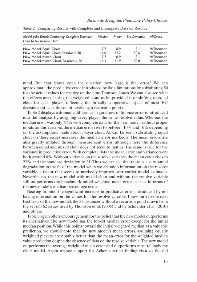
Table 2 helps set the stage for the analyses that follow. As I have emphasized, beyond the data on the nine issues provided to me by Robert Thomson, I do not have an estimate of the new model’s resolve variable and so am reduced to arbitrarily setting its initial value at 50. Because this undoubtedly introduces error, it is important in examining all subsequent results to keep that source of error in

Table 1. Error Rates Across Models, Thomson’s Data Include the Resolve Variable

Model (Abs Error) Median Mean Std Deviation N/Cases

new Model, equal Clout 7.7 8.9 8.1 9/Thomsonnew Model, Mixed Clout 7.7 8.9 8.1 9/ThomsonOld Model, equal Clout 18.5 21.5 19.0 9/ThomsonOld Model, Mixed Clout 18.5 21.5 19.0 9/ThomsonMeDIAn ROunD 1 20.0 29.4 33.7 9/ThomsonMeAn ROunD 1, equal Clout 12.5 11.8 9.8 9/ThomsonMeAn ROunD 1, Mixed Clout 12.5 11.8 9.8 9/Thomson


15

mind. But that leaves open the question, how large is that error? We can approximate the predictive error introduced by data limitations by substituting 50 for the actual values for resolve on the nine Thomson issues. We can also see what the effects are of using the weighted clout as he provided it or shifting to equal clout for each player, reflecting the broadly cooperative aspect of most EU decisions (at least those not involving a recursion point).

Table 2 displays a dramatic difference in goodness of fit once error is introduced into the analysis by assigning every player the same resolve value. Whereas the median error was only 7.7% with complete data for the new model, without proper inputs on this variable, the median error rises to between 10% and 16% depending on the assumptions made about player clout. As can be seen, substituting equal clout on these issues increases the median error markedly. The mean errors are also greatly inflated through measurement error, although here the difference between equal and mixed clout does not seem to matter. The same is true for the variance in predictive error. With complete data the mean error and variance were both around 8%. Without variance on the resolve variable, the mean error rises to 22% and the standard deviation to 31. Thus we can see that there is a substantial degradation in the fit of the model when we abandon information on the resolve variable, a factor that seems to markedly improve over earlier model estimates. Nevertheless, the new model with mixed clout and without the resolve variable still outperforms the benchmark initial weighted mean error at least in terms of the new model’s median percentage error.

Bearing in mind the significant increase in predictive error introduced by not having information on the values for the resolve variable, I now turn to the next best tests of the new model, the 37 instances without a recursion point drawn from the set of 162 issues used by Thomson et al. (2006) and by Schneider et al. (2010) and others.

Table 3 again offers encouragement for the belief that the new model outperforms its alternatives. The new model has the lowest median error except for the initial median position. While this points toward the initial weighted median as a valuable prediction, we should note that the new model’s mean errors, assuming equally weighted players, are notably better than the mean error for the weighted median value prediction despite the absence of data on the resolve variable. The new model outperforms the average weighted mean error and outperforms most tellingly my older model. Again we see support for Achen’s earlier finding vis-à-vis the old

Table 2. Comparing Results with Complete and Incomplete Data on Resolve

Model (Abs Error): Comparing Complete Thomson Data To No Resolve Data

Median Mean Std Deviation N/Cases

new Model, equal Clout 7.7 8.9 8.1 9/Thomsonnew Model, equal Clout, Resolve = 50 16.0 22.2 30.6 9/Thomsonnew Model, Mixed Clout 7.7 8.9 8.1 9/Thomsonnew Model, Mixed Clout, Resolve = 50 10.1 21.9 30.8 9/Thomson


16

model, but that support is absent when applied to the new model even though there is significant known measurement error for the new model.

Table 4 directs our attention to a broader set of cases that might, nevertheless, reflect a somewhat more competitive environment than the total set. That is, Table 4 assesses the fit between models and outcomes for the cases that were classified as new issues rather than amendments. Once again, the new model (with equal clout) achieves the best median error rate and also the best mean error rate while also having the lowest variance in errors among the models tested here.

The results in Tables 3 and 4 highlight an additional factor that is important to keep in mind as we work through the findings. The error rates in these two tables, though higher than in Table 1, are still quite low, especially when looked at from the perspective of median errors. We will see the error rates increase as we leave these initial analyses. The farther we move from a non-cooperative setting into a more purely cooperative, repeated game environment—such as typifies most European Union decision making—the more likely it is that my iterated, but not repeated game models will fare less well. Thus, we are moving to especially difficult tests because the domain of issues is not a good conceptual fit for my old or new model and, in the case of the new model, we are, of course, missing a crucial input, assigning a fixed value where there should be variation in resolve.

Table 5 examines the errors of prediction across the models for the entire 162 cases used in The European Union Decides. Here, with maximal impact of

Table 3. No Resolve Data, Issues without a Recursion Point; Likely to be Less Cooperative


new Model, equal Clout 8.2 16.9 24.8 37/no Recursionnew Model, Mixed Clout 8.2 19.7 28.6 37/no RecursionOld Model, equal Clout 10.0 29.4 35.3 37/no RecursionOld Model, Mixed Clout 10.0 28.2 34.7 37/no RecursionMeDIAn ROunD 1 5.0 19.8 29.8 37/no RecursionMeAn ROunD 1, equal Clout 8.6 19.4 28.0 37/no RecursionMeAn ROunD 1, Mixed Clout 8.5 19.7 28.6 37/no Recursion

Table 4. No Resolve Data, Issues Classified as New; Likely to be Less Cooperative


new Model, equal Clout 12.9 23.4 27.0 111/newnew Model, Mixed Clout18.9 18.9 28.0 30.4 111/newOld Model, equal Clout 20.0 31.1 32.1 111/newOld Model, Mixed Clout 24.4 31.3 32.0 111/newMeDIAn ROunD 1 20.0 27.9 30.6 111/newMeAn ROunD 1, equal Clout 14.5 23.8 27.6 111/newMeAn ROunD 1, Mixed Clout 16.6 24.7 28.8 111/new


17

measurement error and with competitive models misfit to a largely cooperative database, we find an advantage for the new model when viewed from the perspective of its median percentage error (12.7%) compared to the initial median error based on the mean prediction without strategic interplay (14%). The mean predicted errors and standard deviations of the errors are essentially the same. The new model, facing the same challenges as my old, expected utility, model in terms of the cooperative environment, but suffering also from the misspecified resolve variable, nevertheless clearly outperforms the old model and the initial median predicted value. The median and mean error percentages for the new model are substantially lower than for the old model.

A recent study by Schneider et al. (2010) tests additional models using the same data set. They report mean average errors for their best fitting model (the Saliency Nash Bargaining Solution) that improve upon the mean average errors reported here for my new model. For instance, on the full 162 cases, they show a mean average error of 19.5% which is an improvement over my new model’s mean average error of 22.8%. Unfortunately they do not also report median errors or standard deviations. This makes it difficult to assess how important the differences are in mean errors between their best model and the models examined here.

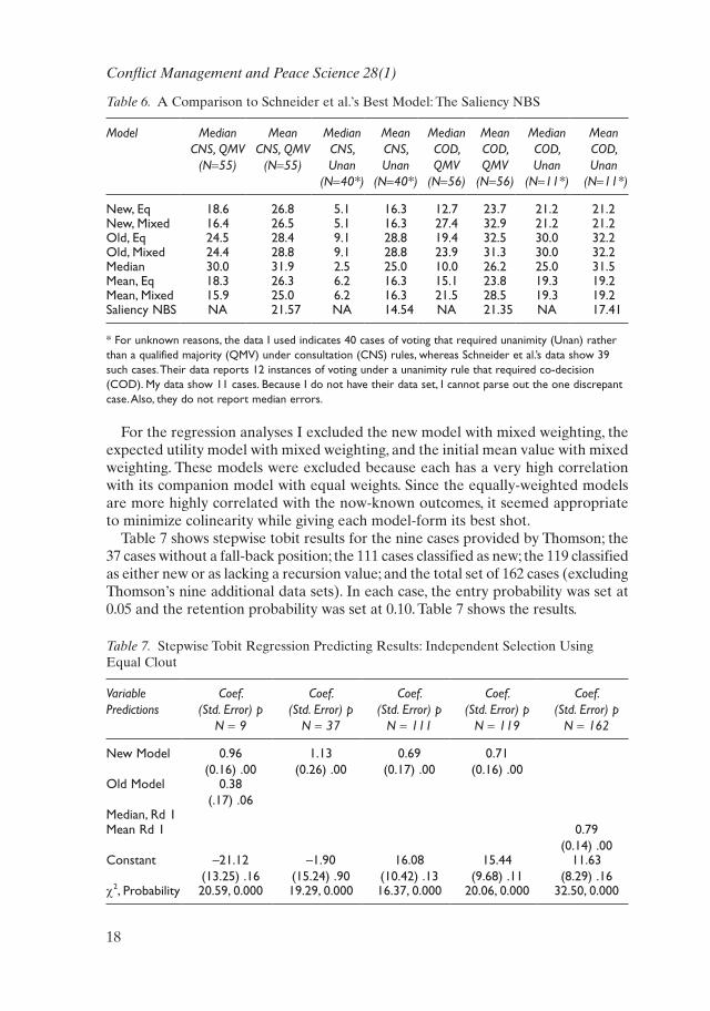
Table 6 reports further comparisons based on their division of the data along formal lines of decision making as explained in the note to the table. I do not have their computed values and so cannot divide their data along the lines I have done in the earlier tables (by recursion value or amendment value) so I must rely only on the divisions they have utilized. These institutional divisions are not substantively as interesting for my non-repeated game models as the divisions reported earlier, but they are what are currently available to me. As Table 6 shows, there often is a substantial difference between the mean average error and the median error in these divisions. This means that the errors are not normally distributed so that a few outliers may be inflating the mean average error while leaving the median unaffected. Which is the better way to calibrate errors in prediction is, of course, a matter of judgment.

Finally, we can ask how well each of the predictive approaches reported here does in a regression sense. Here is an instance for which an atheoretical, stepwise tobit regression (to capture the upper and lower boundary censoring of regression results to fall between 0 and 100) can be especially helpful. Stepwise tobit regression can be used to select for us the model or models that do best at explaining variance in the known results.

Table 5. Tests with Maximal Measurement Error for the New Model


new Model, equal Clout 12.7 22.8 25.9 162/ eu Decidesnew Model, Mixed Clout 16.2 25.8 28.6 162/ eu DecidesOld model, equal Clout 20.5 30.2 31.1 162/ eu DecidesOld Model, Mixed Clout 20.5 30.0 31.2 162/ eu DecidesMeDIAn ROunD 1 20.0 28.2 30.7 162/ eu DecidesMeAn ROunD 1, equal Clout 14.4 22.5 25.5 162/ eu DecidesMeAn ROunD 1, Mixed Clout 14.0 23.7 27.5 162/ eu Decides


18

For the regression analyses I excluded the new model with mixed weighting, the expected utility model with mixed weighting, and the initial mean value with mixed weighting. These models were excluded because each has a very high correlation with its companion model with equal weights. Since the equally-weighted models are more highly correlated with the now-known outcomes, it seemed appropriate to minimize colinearity while giving each model-form its best shot.

Table 7 shows stepwise tobit results for the nine cases provided by Thomson; the 37 cases without a fall-back position; the 111 cases classified as new; the 119 classified as either new or as lacking a recursion value; and the total set of 162 cases (excluding Thomson’s nine additional data sets). In each case, the entry probability was set at 0.05 and the retention probability was set at 0.10. Table 7 shows the results.

Table 6. A Comparison to Schneider et al.’s Best Model: The Saliency NBS

Model MedianCNS, QMV

(N=55)

MeanCNS, QMV

(N=55)

MedianCNS,Unan

(N=40*)

MeanCNS,Unan

(N=40*)

MedianCOD,QMV

(N=56)

MeanCOD,QMV

(N=56)

MedianCOD,Unan

(N=11*)

MeanCOD,Unan

(N=11*)

new, eq 18.6 26.8 5.1 16.3 12.7 23.7 21.2 21.2new, Mixed 16.4 26.5 5.1 16.3 27.4 32.9 21.2 21.2Old, eq 24.5 28.4 9.1 28.8 19.4 32.5 30.0 32.2Old, Mixed 24.4 28.8 9.1 28.8 23.9 31.3 30.0 32.2Median 30.0 31.9 2.5 25.0 10.0 26.2 25.0 31.5Mean, eq 18.3 26.3 6.2 16.3 15.1 23.8 19.3 19.2Mean, Mixed 15.9 25.0 6.2 16.3 21.5 28.5 19.3 19.2Saliency nBS nA 21.57 nA 14.54 nA 21.35 nA 17.41

* For unknown reasons, the data I used indicates 40 cases of voting that required unanimity (unan) rather than a qualified majority (qMV) under consultation (CnS) rules, whereas Schneider et al.’s data show 39 such cases. Their data reports 12 instances of voting under a unanimity rule that required co-decision (COD). My data show 11 cases. Because I do not have their data set, I cannot parse out the one discrepant case. Also, they do not report median errors.

Table 7. Stepwise Tobit Regression Predicting Results: Independent Selection Using Equal Clout

Variable Predictions

Coef. (Std. Error) p

N = 9


N = 37


N = 111


N = 119


N = 162

new Model 0.96 (0.16) .00

1.13 (0.26) .00

0.69 (0.17) .00

0.71 (0.16) .00

Old Model 0.38 (.17) .06

Median, Rd 1Mean Rd 1 0.79

(0.14) .00Constant –21.12

(13.25) .16–1.90

(15.24) .9016.08

(10.42) .1315.44

(9.68) .1111.63

(8.29) .16χ2, Probability 20.59, 0.000 19.29, 0.000 16.37, 0.000 20.06, 0.000 32.50, 0.000


19

Table 7 provides additional encouragement and confidence in the new model introduced here. The new model appears in the final regression results in every case except the test on all 162 issues, including those that reflect most strongly the European Union’s repeated game, cooperative environment. The initial weighted mean predicted value is the only significant model in that case. In the absence of a recursion point, the expected utility model also plays a part in explaining the value of the actual issue results although its statistical significance is beyond conventional levels. So, despite the benefits from simply taking an initial weighted mean value as the predicted outcome, adding the complexity of strategic interaction contributes significantly and substantively to the accuracy of prediction in the most relevant cases according to these findings and this is so despite the significant known addition of measurement error on the resolve variable.

We can add a tougher test, more aligned with sorting out Achen’s contention that complex models add little beyond simply calculating the weighted mean position on the issues (remembering, of course, that even that calculation relies on the variables defined as essential by the more complex models). Table 8 replicates Table 7, but this time only for cases for which the new model prediction differs from the initial weighted mean prediction. That is a particularly demanding case because that is where the contending models have the greatest opportunity to part from the weighted mean prediction and, therefore, to prove their alleged inferiority (Achen, 2006). Table 8 makes evident that with the exception of one regression analysis, the weighted mean result is not the superior predictor while the new model I have offered almost always is and is so by itself.

Tables 7 and 8 provide insight into several issues. The weighted mean prediction only outperforms the new model in the test that includes cases farthest removed from the competitive, non-cooperative environment for which my models are designed, as was also true in Table 7. Thus, while the tests confirm Achen’s finding for the broad array of European Union issues, in both Tables 7 and 8 Achen’s finding is not supported—despite measurement error induced by the absence of

Table 8. Stepwise Tobit Regression: Excludes Cases for which New Model Prediction = Weighted Mean Prediction, All Based on Equal Clout

Variable Predictions

No Recursion PointCoef. , Std. Error, p

N = 26

New Issue Coef., Std. Error, p

N = 69

No Recursion or New Issue

Coef. , Std. Error, pN = 75

All CasesCoef. , Std. Error, p

N = 99

new Model

1.28 (0.31) .00 0.89 (.020) .00 0.85 (0.17) .00

Old ModelMedian Round 1Mean Round 1

0.80 (.17) .00

Constant –13.59 (18.69) .47 5.59 (11.52) .63 7.26 (10.56) .49 11.01 (9.81) .27χ2, Probability

16.34, 0.000 18.91, 0.000 21.23, 0.000 20.98, 0.000


20

data on the resolve variable—when the analysis focuses on more competitive, iterated game issues. In those cases, the new model outperforms the weighted mean prediction and all other models tested here.

ConclusionsI have introduced a new model for predicting and engineering policy outcomes. It has been tested against the expected utility model and against predictions generated solely from the input data without strategic interplay. The tests show that even with substantial measurement error due to missing variance on the resolve variable, the new model outperforms my old model and outperforms the weighted median and weighted mean error rates when the data come closer to the environment for which the new (and old) model were designed; that is, a non-cooperative environment that does not involve indefinite or infinitely repeated play. With complete data for the new model, it substantially outperforms the alternatives. The results encourage the belief that the new model represents a significant improvement over alternative specifications for iterated, non-repeated strategic settings involving the opportunity for negotiation and also for coercion.

In addition to its improved performance relative to alternatives, the new model offers several other advantages. It provides the opportunity to estimate pair-wise salience scores and their changes across iterations, whereas the alternative approaches take salience as fixed for the period of the game and as inherent in the individual player rather than in the dyadic relationship across iterations. The new model also permits an estimation of changes in player influence across iterations, making it possible to predict who is growing or declining in relative clout. Student projects at NYU used this feature, for instance, to identify the growing influence of the Taliban and Al Qaeda within Pakistan about seven months before such a result was reported in the New York Times (Bueno de Mesquita, 2009).

The model presented here is part of a family of models I am currently constructing. I have recently integrated a network analysis capability and estimates of winning coalition and selectorate size into this model, but am also developing a version in which players dynamically enter and exit the game. As these tools become available and are tested I hope to make additional software available for broader academic and classroom use and for academic evaluation. Tests against other models in more diverse settings are also required before any judgment can be made about the circumstances under which different models perform best. For instance, it will be useful to compare the Schneider et al. saliency NBS model to the new model in a broader array of settings, as well as important models being worked on by others.

References

Achen, Christopher. 2006. Evaluating political decisionmaking models. InThe European Union Decides, eds Robert Thomson et al., ch. 10. Cambridge: Cambridge University Press.

Axelrod, Robert. 1970. Conflict of Interest: A Theory of Divergent Goals with Applications to Politics. Chicago, IL: Markham.

Bueno de Mesquita, Bruce. 1984. Forecasting policy decisions: An expected utility approach to post-Khomeini Iran. PS (Spring): 226–236.


21

Bueno de Mesquita, Bruce. 1994. Policy forecasting: An expected utility model. In European Community Decision Making, eds Bruce Bueno de Mesquita and Frans Stokman, pp. 71–104. New Haven, CT: Yale University Press.

Bueno de Mesquita, Bruce. 1998. The end of the Cold War: Predicting an emergent property. Journal of Conflict Resolution 42(2): 131–155.

Bueno de Mesquita, Bruce. 1999 (and subsequent editions). Principles of International Politics. Washington, DC: CQ Press.

Bueno de Mesquita, Bruce. 2002. Predicting Politics. Columbus, OH: Ohio State University Press.

Bueno de Mesquita, Bruce. 2009. The Predictioneer’s Game. New York: Random House.Bueno de Mesquita, Bruce, and David Lalman. 1992. War and Reason. New Haven, CT: Yale

University Press.Bueno de Mesquita, Bruce, and Frans Stokman, eds. 1994. European Community Decision

Making: Models, Applications and Comparisons. New Haven, CT: Yale University Press.Chae, S. and Yang, J.-A. (1994) A N-person pure bargaining game. Journal of Economic

Theory 62(1): 86–102.Feder, Stanley. 1995. FACTIONS and Policon: New ways to analyze politics. In Inside CIA’s

Private World, ed. H. Bradford Westerfield, pp. 274–292. New Haven, CT: Yale University Press,

Feder, Stanley. 2002. Forecasting for policy making in the post-Cold War period. Annual Review of Political Science 5: 111–25.

Garrett, Geoffrey, and George Tsebelis. 2001. Even more reasons to resist the temptation of power indices in the EU. Journal of Theoretical Politics 13(1): 99–105.

Green, Kesten C. 2002. Embroiled in a conflict: Who do you call? International Journal of Forecasting 18(3): 389–395.

Ray, James L., and Bruce M. Russett. 1996. The future as arbiter of theoretical controversies: Predictions, explanations and the end of the Cold War. British Journal of Political Science 26: 441–70.

Schneider, Gerald, Daniel Finke and Stefanie Bailer. 2010. Bargaining power in the European Union: An evaluation of competing game-theoretic models. Political Studies 58(1): 85–103.

Shapin, Steven, and Simon Shaffer. 1989. Leviathan and the Air-Pump: Hobbes, Boyle and the Experimental Life. Princeton, NJ: Princeton University Press.

Sobel, Dava. 2006. The Planets. London: Penguin.Tetlock, Philip E. 2006. Expert Political Judgment. Princeton, NJ: Princeton University Press.Thomson, Robert, Frans N. Stokman, Christopher H. Achen and Thomas König, eds. 2006.

The European Union Decides. Cambridge: Cambridge University Press.

BRuCe BuenO De MeSquITA is the Julius Silver Professor of Politics and Director of the Alexander Hamilton Center for Political economy at new York university and a Senior Fellow at the Hoover Institution at Stanford university. His most recent books include The Predictioneer’s Game (Random House, 2009), The Strategy of Campaigning (with Kiron Skinner, Serhiy Kudelia, and Condoleezza Rice, university of Michigan Press, 2007), and The Logic of Political Survival (with Alastair Smith, Randolph Siverson, and James Morrow, MIT Press, 2003, selected as the best book in 2002–2003 on conflict by the Conflict Processes section of the American Political Science Association and as Choice Outstanding Academic Title for 2004).

A New Model for Predicting Policy Choices

Documents

Transcript of A New Model for Predicting Policy Choices