ORIGINAL PAPER

A new mathematical model for horizontal wells with variabledensity perforation completion in bottom water reservoirs

Dian-Fa Du1 • Yan-Yan Wang2 • Yan-Wu Zhao1 • Pu-Sen Sui3 • Xi Xia1

Received: 11 July 2016 / Published online: 12 April 2017

� The Author(s) 2017. This article is an open access publication

Abstract Horizontal wells are commonly used in bottom

water reservoirs, which can increase contact area between

wellbores and reservoirs. There are many completion

methods used to control cresting, among which variable

density perforation is an effective one. It is difficult to

evaluate well productivity and to analyze inflow profiles of

horizontal wells with quantities of unevenly distributed

perforations, which are characterized by different param-

eters. In this paper, fluid flow in each wellbore perforation,

as well as the reservoir, was analyzed. A comprehensive

model, coupling the fluid flow in the reservoir and the

wellbore pressure drawdown, was developed based on

potential functions and solved using the numerical discrete

method. Then, a bottom water cresting model was estab-

lished on the basis of the piston-like displacement princi-

ple. Finally, bottom water cresting parameters and factors

influencing inflow profile were analyzed. A more system-

atic optimization method was proposed by introducing the

concept of cumulative free-water production, which could

maintain a balance (or then a balance is achieved) between

stabilizing oil production and controlling bottom water

cresting. Results show that the inflow profile is affected by

the perforation distribution. Wells with denser perforation

density at the toe end and thinner density at the heel end

may obtain low production, but the water breakthrough

time is delayed. Taking cumulative free-water production

as a parameter to evaluate perforation strategies is advis-

able in bottom water reservoirs.

Keywords Bottom water reservoirs � Variable density

perforation completion � Inflow profile � Cresting model �Cumulative free-water production

1 Introduction

Bottom water reservoirs are widely distributed on earth and

hold a large proportion of oil reserves (Islam 1993). Taking

China for example, there exist a large number of bottom

water reservoirs, most of which are developed using hori-

zontal wells. Compared with vertical wells, the producing

sections of horizontal wells have direct contact with oil

reservoirs, which not only reduces the producing pressure

drawdown, but also ensures bottom water flowing into the

wellbore more smoothly in a form of ‘‘pushing upward’’

(Besson and Aquitaine 1990; Dou et al. 1999; Permadi

et al. 1996; Zhao et al. 2006). Owing to these advantages, it

can effectively control bottom water cresting. The need of

economic and effective development of bottom water

reservoirs leads to the appearance of many types of com-

pletion methods, such as barefoot well completion, slotted

screen well completion and perforation completion

(Ouyang and Huang 2005). Recently, partial completion,

variable density perforation completion and other new

completion methods have been put forward to further

control bottom water cresting (Goode and Wilkinson 1991;

Sognesand et al. 1994). By accurately finding out the water

& Dian-Fa Du

dudf@upc.edu.cn

& Yan-Yan Wang

514375721@qq.com

1 School of Petroleum Engineering, China University of

Petroleum, Qingdao 266580, Shandong, China

2 Sinopec Petroleum Exploration and Production Research

Institute, Sinopec, Beijing 100083, China

3 Shengli Production Plant, Shengli Oilfield Branch Company,

Sinopec, Dongying 257051, Shandong, China

Edited by Yan-Hua Sun

123

Pet. Sci. (2017) 14:383–394

DOI 10.1007/s12182-017-0159-0

production interval of horizontal wells, adopting plugging

strategies or properly adjusting the bottom water inflow

profile, these techniques can effectively prolong the life of

production wells. And among all these techniques, perfo-

ration completion, including variable density perforation

and selectively perforated completion, plays a critical role

in alleviating water cresting (Pang et al. 2012).

Previously, scholars put more emphasis on the produc-

tivity evaluation of horizontal wells (Dikken 1990; Novy

1995; Penmatcha et al. 1998) and bottom water cresting

(Permadi et al. 1995; Wibowo et al. 2004; Chaperon 1986).

The published papers mostly focused on horizontal wells

with open-hole completion. There is little research into

horizontal wells with variable density perforation comple-

tion, and the ones that exist turned out to be very prob-

lematic: (1) The method for open-hole completion

horizontal wells was used ignoring the fluid flow in per-

foration tunnels in these studies (Landman and Goldthorpe

1991; Yuan et al. 1996; Zhou et al. 2002). Then, a model

describing the damage zone must be introduced to char-

acterize the influence of perforation holes (Umnuaypon-

wiwat and Ozkan 2000; Muskat and Wycokoff 2013).

Some scholars utilized the numerical simulation method to

discuss the impact of selective perforation on the produc-

tivity of horizontal wells and built a single-phase flow

variable density perforation model for horizontal wells by

two filtration zones (Li et al. 2010). Since the seepage

resistance needs to be considered more precisely, espe-

cially in the middle and later periods of the oilfield

development, the existing results are somewhat inaccurate.

(2) Conventional simplified models cannot analyze for-

mation pressure thoroughly and predict bottom water

cresting. Furthermore, a non-uniformly distributed bottom

water inflow profile along the wellbore was obtained

without considering the wellbore pressure drop (Guo et al.

1992). (3) In order to optimize completion parameters for

horizontal wells, oil production is usually viewed as the

only objective function. It is reasonable for horizontal wells

in conventional reservoirs. However, it is not accurate for

horizontal wells located in bottom water reservoirs because

of ignoring bottom water cresting, which decreases the

effective production period of wells (Luo et al. 2015).

In this paper, based on the precise consideration of the

fluid flow in each perforation, the flow behavior in perfo-

rations, wellbores, as well as reservoirs, was analyzed.

Coupling the fluid flow in reservoirs and wellbore pressure

drop, a comprehensive model, which can be used to eval-

uate productivity of horizontal wells, was developed based

on potential functions and solved using the numerical

discrete method. Then, a model describing bottom water

cresting was established on the basis of the piston-like

displacement principle. Finally, both the bottom water

cresting behavior and the factors influencing inflow profile

were analyzed using the developed model, and a more

systematic optimization method was proposed by intro-

ducing the concept of the cumulative free-water produc-

tion, which could realize a balance between stabilizing oil

production and controlling bottom water coning.

2 Productivity analysis for horizontal wellswith variable density perforation completion

For horizontal wells with perforation completed in bottom

water reservoirs, formation fluids firstly flow into perfora-

tion holes before converging in the horizontal wellbore.

Under this circumstance, the effect of perforation holes is

similar to that of short producing branches in inclined

horizontal wells (Holmes et al. 1998). The real producing

part for horizontal wells should be quantities of perforation

holes. Therefore, the perforation holes can be regarded as

‘‘source-sink’’ term, and this kind of problem can be solved

with a source function.

2.1 Analysis of fluid flow near wellbore regions

A model was built to describe the flow of formation fluid

near horizontal wellbores, and the assumptions for this

model are as follows:

(1) The formation is homogeneous with a uniform

thickness;

(2) The horizontal permeability meets the following

basic relationship: Kx = Ky = Kh, and the vertical

permeability is Kz = Kv. The target reservoir is

infinite in the horizontal plane;

(3) The single-phase fluid flowing in the reservoir is

incompressible and the fluid flow obeys Darcy’s law;

(4) The wellbore is horizontal, in which the perforations

are unevenly distributed;

(5) The perforating direction is perpendicular to the

wellbore, and the lengths as well as radius of all the

perforation tunnels are the same.

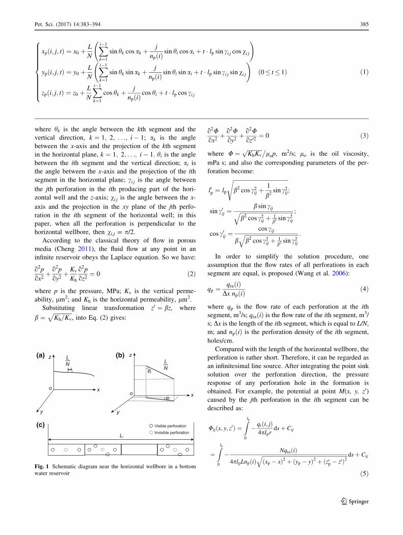
Acoordinate system is established as shown in Fig. 1, in

which the heel end of the wellbore is M0 (x0, y0, z0). The

horizontal part of the wellbore (total length L, m) is divided

into N segments. Therefore, the length of each segment is

L/N.

Different segments have different characteristic

parameters: the perforation density, np(i); the perforation

depth, lp; bore diameter, Dp; phase angle x; and the initial

perforation angle x0. The heel end is selected as the

origin of this coordinate, and the x direction is parallel

with the wellbore. The coordinates of any point (x, y, z) in

the jth perforation tunnel in the ith segment are as fol-

lows:

384 Pet. Sci. (2017) 14:383–394

123

where hk is the angle between the kth segment and the

vertical direction, k ¼ 1; 2; . . .; i� 1; ak is the angle

between the x-axis and the projection of the kth segment

in the horizontal plane, k ¼ 1; 2; . . .; i� 1. hi is the angle

between the ith segment and the vertical direction; ai isthe angle between the x-axis and the projection of the ith

segment in the horizontal plane; ci j is the angle between

the jth perforation in the ith producing part of the hori-

zontal well and the z-axis; vi j is the angle between the x-

axis and the projection in the xy plane of the jth perfo-

ration in the ith segment of the horizontal well; in this

paper, when all the perforation is perpendicular to the

horizontal wellbore, then vi,j = p/2.According to the classical theory of flow in porous

media (Cheng 2011), the fluid flow at any point in an

infinite reservoir obeys the Laplace equation. So we have:

o2p

ox2þ o2p

oy2þ Kv

Kh

o2p

oz2¼ 0 ð2Þ

where p is the pressure, MPa; Kv is the vertical perme-

ability, lm2; and Kh is the horizontal permeability, lm2.

Substituting linear transformation z0 ¼ bz, where

b ¼ffiffiffiffiffiffiffiffiffiffiffiffiffi

Kh=Kv

p

, into Eq. (2) gives:

o2Uox2

þ o2Uoy2

þ o2Uoz02

¼ 0 ð3Þ

where U ¼ffiffiffiffiffiffiffiffiffiffiffi

KhKv

p �

lop, m2/s; lo is the oil viscosity,

mPa s; and also the corresponding parameters of the per-

foration become:

l0p ¼ lp

ffiffiffiffiffiffiffiffiffiffiffiffiffiffiffiffiffiffiffiffiffiffiffiffiffiffiffiffiffiffiffiffiffiffiffiffiffiffiffi

b2 cos c2ij þ1

b2sin c2ij

s

;

sin c0ij ¼b sin cij

ffiffiffiffiffiffiffiffiffiffiffiffiffiffiffiffiffiffiffiffiffiffiffiffiffiffiffiffiffiffiffiffiffiffiffiffiffiffi

b2 cos c2ij þ 1b2sin c2ij

q ;

cos c0ij ¼cos cij

bffiffiffiffiffiffiffiffiffiffiffiffiffiffiffiffiffiffiffiffiffiffiffiffiffiffiffiffiffiffiffiffiffiffiffiffiffiffi

b2 cos c2ij þ 1b2sin c2ij

q :

In order to simplify the solution procedure, one

assumption that the flow rates of all perforations in each

segment are equal, is proposed (Wang et al. 2006):

qp ¼qraðiÞ

Dx npðiÞð4Þ

where qp is the flow rate of each perforation at the ith

segment, m3/s; qraðiÞ is the flow rate of the ith segment, m3/

s; Dx is the length of the ith segment, which is equal to L/N,

m; and npðiÞ is the perforation density of the ith segment,

holes/cm.

Compared with the length of the horizontal wellbore, the

perforation is rather short. Therefore, it can be regarded as

an infinitesimal line source. After integrating the point sink

solution over the perforation direction, the pressure

response of any perforation hole in the formation is

obtained. For example, the potential at point M(x, y, z0)caused by the jth perforation in the ith segment can be

described as:

Uijðx; y; z0Þ ¼Z

lp

0

� qrði; jÞ4plpr

dsþ Cij

¼Z

lp

0

� NqraðiÞ

4plpLnpðiÞffiffiffiffiffiffiffiffiffiffiffiffiffiffiffiffiffiffiffiffiffiffiffiffiffiffiffiffiffiffiffiffiffiffiffiffiffiffiffiffiffiffiffiffiffiffiffiffiffiffiffiffiffiffiffiffiffiffiffiffiffiffiffiffiffiffi

ðxp � xÞ2 þ ðyp � yÞ2 þ ðz0p � z0Þ2q dsþ Cij

ð5Þ

xpði; j; tÞ ¼ x0 þL

N

X

i�1

k¼1

sin hk cos ak þj

npðiÞsin hi cos ai þ t � lp sin ci j cos vi j

!

ypði; j; tÞ ¼ y0 þL

N

X

i�1

k¼1

sin hk sin ak þj

npðiÞsin hi sin ai þ t � lp sin ci j sin vi j

!

ð0� t� 1Þ

zpði; j; tÞ ¼ z0 þL

N

X

i�1

k¼1

cos hk þj

npðiÞcos hi þ t � lp cos ci j

8

>

>

>

>

>

>

>

>

>

<

>

>

>

>

>

>

>

>

>

:

ð1Þ

LN

z

y

xo

o

θi

αi

z

y

x

(a)

(c)

Li

(b)LN

Visible perforation

Invisible perforation

Fig. 1 Schematic diagram near the horizontal wellbore in a bottom

water reservoir

Pet. Sci. (2017) 14:383–394 385

123

The integration of Eq. (5) is as follows:

Uijðx; y; z0Þ ¼ � NqraðiÞ4plpLnpðiÞ

lnr1ij þ r2ij þ l0pr1ij þ r2ij � l0p

þ Cij ð6Þ

where qr(i, j) is the flow rate of the jth perforation tunnel in

the ith segment, m3/s; r is the distance between the source

point Mpðx; y; z0Þ and the target point Mðx; y; z0Þ; Cij is an

integration constant; r1ij is the distance between the heel

end and the target point; r2ij is the distance between the toe

end and the target point, and they observe the following

expressions, respectively:

r1ij ¼ffiffiffiffiffiffiffiffiffiffiffiffiffiffiffiffiffiffiffiffiffiffiffiffiffiffiffiffiffiffiffiffiffiffiffiffiffiffiffiffiffiffiffiffiffiffiffiffiffiffiffiffiffiffiffiffiffiffiffiffiffiffiffiffiffiffiffiffiffiffiffiffiffiffiffiffiffiffiffiffiffiffiffiffiffiffiffiffiffiffiffiffiffiffiffiffiffiffiffiffiffi

½xpði; j; 0Þ � x�2 þ ½ypði; j; 0Þ � y�2 þ ½z0pði; j; 0Þ � z0�2q

ð7Þ

r2ij ¼ffiffiffiffiffiffiffiffiffiffiffiffiffiffiffiffiffiffiffiffiffiffiffiffiffiffiffiffiffiffiffiffiffiffiffiffiffiffiffiffiffiffiffiffiffiffiffiffiffiffiffiffiffiffiffiffiffiffiffiffiffiffiffiffiffiffiffiffiffiffiffiffiffiffiffiffiffiffiffiffiffiffiffiffiffiffiffiffiffiffiffiffiffiffiffiffiffiffiffiffiffiffi

½xpði; j; 1Þ � x�2 þ ½ypði; j; 1Þ � y�2 þ ½z0pði; j; 1Þ � z0�2q

ð8Þ

where xp(i, j, 0), yp(i, j, 0), zp(i, j, 0) and xp(i, j, 1), yp(i, j, 1),

zp(i, j, 1) are the coordinates of the left and right ends of the

jth perforation in the ith producing part.

Based on the mirror image reflection and superposition

principle, the potential of the jth perforation tunnel for

the ith production segment at point Mpðx; y; z0Þ is

obtained:

Uðx;y;z0Þ ¼� NqraðiÞ4plpLnpðiÞ

X

þ1

n¼�1nij�

ð2h0 þ4nh0 � z0pijði; j;0Þ;

2h0 þ4nh0 � z0pijði; j;1Þ; x; y; z0Þþ nijð4nh0 þ z0pijði; j;0Þ; 4nh0 þ z0pijði; j;1Þ; x ;y;z0Þ�nijð�2h0 þ4nh0 þ z0pijði; j;0Þ ;�2h0

þ4nh0 þ z0pijði; j;1Þ; x ;y ;z0Þ� nijð4nh0 � z0pijði; j;0Þ; 4nh0

� z0pijði; j;1Þ; x ;y ;z0ÞþC0i

�

ð9Þ

with

nijðe0; e1; x; y; z0Þ ¼ lnr1ij þ r2ij þ l0pr1i þ r2i � l0p

ð10Þ

r1i ¼ffiffiffiffiffiffiffiffiffiffiffiffiffiffiffiffiffiffiffiffiffiffiffiffiffiffiffiffiffiffiffiffiffiffiffiffiffiffiffiffiffiffiffiffiffiffiffiffiffiffiffiffiffiffiffiffiffiffiffiffiffiffiffiffiffiffiffiffiffiffiffiffiffiffiffiffiffiffiffiffiffiffiffiffiffi

½xði; j; 0Þ � x�2 þ ½yði; j; 0Þ � y�2 þ ½e0 � z0�2q

ð11Þ

r2i ¼ffiffiffiffiffiffiffiffiffiffiffiffiffiffiffiffiffiffiffiffiffiffiffiffiffiffiffiffiffiffiffiffiffiffiffiffiffiffiffiffiffiffiffiffiffiffiffiffiffiffiffiffiffiffiffiffiffiffiffiffiffiffiffiffiffiffiffiffiffiffiffiffiffiffiffiffiffiffiffiffiffiffiffiffiffi

½xði; j; 1Þ � x�2 þ ½yði; j; 1Þ � y�2 þ ½e1 � z0�2q

ð12Þ

According to the superposition principle, the potential at

any point of the infinite formation created by all the per-

foration tunnels of the horizontal well is:

Uijðx; y; z0Þ ¼ � N

4plpL

X

N

i¼1

qraðiÞnpðiÞ

X

LNnpðiÞ

j¼1

ln/ij þ C ð13Þ

with

/ij ¼X

þ1

n¼�1

(

nij�

2h0 þ 4nh0 � z0pijði; j; 0Þ; 2h0 þ 4nh0

�z0pijði; j; 1Þ; x; y; z0�

þ nij�

4nh0 þ z0pijði; j; 0Þ; 4nh0

þz0pijði; j; 1Þ; x; y; z0�

� nij�

�2h0 þ 4nh0 þ z0pijði; j; 0Þ;�2h0

þ4nh0 þ z0pijði; j; 1Þ; x; y; z0�

� nij 4nh0 � z0pijði; j; 0Þ; 4nh0 � z0pijði; j; 1Þ; x; y; z0� �

þ 2lp

nh0

)

C0i

ð14Þ

The boundary pressure at the oil–water interface is

assumed to be constant. Therefore, the potential at any

point of the formation may be expressed as:

Uijðx; y; z0Þ ¼ Ue �N

4plpL

X

N

i¼1

qraðiÞnpðiÞ

X

LNnpðiÞ

j¼1

ln/ij ð15Þ

Combining the definition of potential, the pressure at

any point of the formation can be given as follows:

pwf;ijðx; y; z0Þ ¼ pe �Nlo

4plpLffiffiffiffiffiffiffiffiffiffiffi

KhKv

pX

N

i¼1

qraðiÞnpðiÞ

X

LNnpðiÞ

j¼1

ln/ij

ð16Þ

where pe is the boundary pressure, MPa.

For perforated completion, the perforation tunnels

directly contact the formation. Therefore, the flow potential

of some point, which is just located in the perforation, can be

obtained using Eq. (15). In this case, there are two points

involved: the target point and the source point (perforation

point). To get rid of singularity phenomenon, the central hole

in thewall is chosen as the jth perforation’s target point when

calculating the distance between two perforation points.

Only calculating the pressure of one central point for the

segment and regarding it as the pressure of the whole

segment will result in deviation when analyzing the seg-

ment’s pressure of a horizontal wellbore. In this paper,

taking the average over all the perforations’ pressure in the

same segment and using the average value as the repre-

sentative pressure of that segment, the pressure of the ith

segment is as follows:

pwfðiÞ ¼1

Dx npðiÞX

Dx npðiÞ

j¼1

pwfði; jÞ ð17Þ

where pwf(i) is the flow pressure for all the perorations in

the ith segment, MPa.

386 Pet. Sci. (2017) 14:383–394

123

There are 2N variables required to be calculated by

analyzing pressure distribution along the wellbore: pwf(i)

and qra(i), (i = 1, 2, …, N). However, it only contains

N equations in the flow model [Eq. (15)]. Therefore, one

more model is needed to describe pressure drop along the

wellbore (Li et al. 1996, 2006).

2.2 Wellbore pressure drop model

For perforated horizontal wells, the main idea to develop a

wellbore pressure drop model is to divide the horizontal

wellbore into several segments, and each segment is sub-

divided into several smaller parts that only include one

perforation (Su and Gudmundsson 1994).

According to the analysis of the pressure drop in a

wellbore, the total pressure loss can be written as:

dpwfðiÞ ¼ dpfricðiÞ þ dpaccðiÞ þ dpmixðiÞ þ dpGðiÞ ð18Þ

where dpfric(i) is the friction loss of the ith segment, MPa;

dpacc(i) is the acceleration loss of the ith segment, MPa;

dpmix(i) is the mixing loss of the ith segment, MPa; and

dpG(i) is the gravity loss of the ith segment, MPa.

It should be noted that, in the previous section, a

mechanical field described by the flow model is estab-

lished based on the potential function. Therefore, when

the potential function is used to deal with flow problems,

the pressure loss caused by viscous force has been con-

sidered. As we all know, the mathematical expression of

fluid potential is Kp/l, where K is the formation perme-

ability, p represents pressure, while l means the fluid

viscosity, and it is used to describe the viscous force,

which will lead to pressure loss along the perforation. So

it means that the viscous force has been taken into con-

sideration in the first model. In other words, when

building wellbore pressure here, only four kinds of pres-

sure loss should be calculated.

The calculation method of frictional loss and accelera-

tion loss between two perforation tunnels is expressed,

respectively.

Dpfric ¼ 1:34� 10�13ffricði; jÞDlD

q�v2s ði; jÞ2

¼ 1:0862� 10�13ffricði; jÞqq2Lði; jÞD5npðiÞ

ð19Þ

Dpaccði; jÞ ¼ q �v2s i; jð Þ � �v2s ði; jþ 1Þ�

¼ 3:5215� 10�13 qD5

q2Lði; jÞ � q2Lði; jþ 1Þ�

ð20Þ

where q is the liquid density, kg/m3; D is the wellbore

diameter, m; qL(i,j) is the flow rate along the wellbore, m3/

d; �vsði; jÞ is the average velocity of the jth perforation in the

ith segment, m/s; and ffricði; jÞ is the friction coefficient of

the jth perforation in the ith segment.

In Eq. (19), one parameter, called the friction coeffi-

cient, is introduced. The calculation of the friction coeffi-

cient is dependent on the Reynolds number. If the Reynolds

number is less than or equal to 2000, the flow is laminar;

otherwise, it is turbulent flow. And the expression for the

Reynolds number is as follows:

Re ¼ 7:3682844� 10�3 Qqrl

where Re is the Reynolds number; Q is the axial flow rate

along the wellbore, m3/d; l is the viscosity of the flowing

fluid, mPa s; and r is the wellbore radius, m.

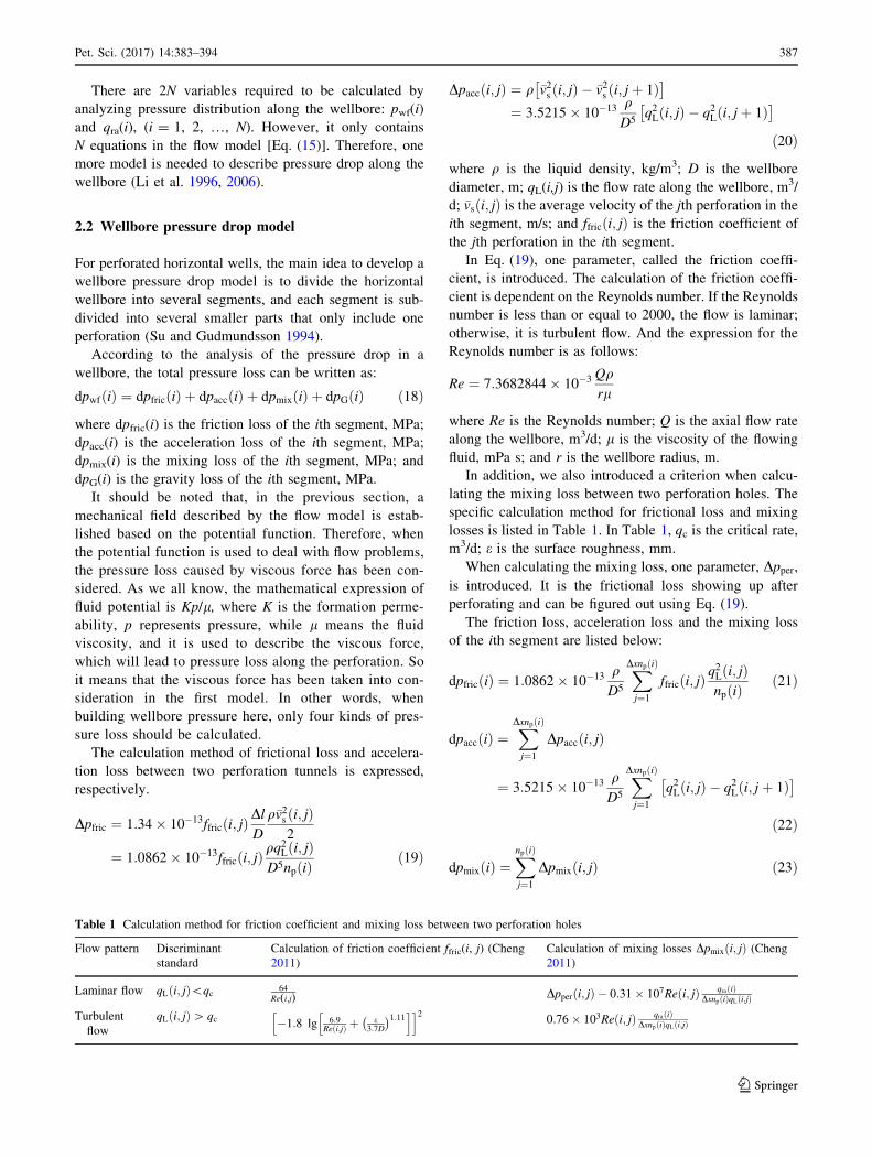
In addition, we also introduced a criterion when calcu-

lating the mixing loss between two perforation holes. The

specific calculation method for frictional loss and mixing

losses is listed in Table 1. In Table 1, qc is the critical rate,

m3/d; e is the surface roughness, mm.

When calculating the mixing loss, one parameter, Dpper,is introduced. It is the frictional loss showing up after

perforating and can be figured out using Eq. (19).

The friction loss, acceleration loss and the mixing loss

of the ith segment are listed below:

dpfricðiÞ ¼ 1:0862� 10�13 qD5

X

DxnpðiÞ

j¼1

ffricði; jÞq2Lði; jÞnpðiÞ

ð21Þ

dpaccðiÞ ¼X

DxnpðiÞ

j¼1

Dpaccði; jÞ

¼ 3:5215� 10�13 qD5

X

DxnpðiÞ

j¼1

q2Lði; jÞ � q2Lði; jþ 1Þ�

ð22Þ

dpmixðiÞ ¼X

npðiÞ

j¼1

Dpmixði; jÞ ð23Þ

Table 1 Calculation method for friction coefficient and mixing loss between two perforation holes

Flow pattern Discriminant

standard

Calculation of friction coefficient ffric(i, j) (Cheng

2011)

Calculation of mixing losses Dpmixði; jÞ (Cheng2011)

Laminar flow qLði; jÞ\qc 64

Re(i;j) Dpperði; jÞ � 0:31� 107Reði; jÞ qraðiÞDxnpðiÞqLði;jÞ

Turbulent

flow

qLði; jÞ[ qc �1:8 lg 6:9Reði;jÞ þ e

3:7D

�1:11h ih i2

0:76� 103Reði; jÞ qraðiÞDxnpðiÞqLði;jÞ

Pet. Sci. (2017) 14:383–394 387

123

If the horizontal well is inclined, the gravity loss is

non-ignorable, and the wellbore pressure drop model

becomes:

2.3 Coupling model

When a horizontal well begins to produce reservoir fluids,

the fluids in the perforations connect the wellbore and oil

reservoir together. Therefore, perforation is considered as

an infinitesimal linear sink, which directly contacts reser-

voir and wellbore. Meanwhile, pressure responses are

generated in the whole reservoir. The generated pressure

responses near the perforations are associated with oil

inflow in the radial direction of the horizontal wellbore,

which can be calculated by utilizing the reservoir flow

model. Since the pressure in perforation holes is relevant to

the wellbore pressure, a coupling relationship exists

between the reservoir flow model and the wellbore pressure

drop model.

According to the reservoir flow model, a model is

developed to calculate steady-state productivity of the

horizontal well with variable density perforation, in which

the pressure drop along the horizontal wellbore is consid-

ered:

where pwf(i) is the wellbore pressure in the ith segment,

MPa; N is the number of divided segments along the

wellbore; and /kj is a function corresponding to the hori-

zontal wellbore as well as the oil–water interface.

In this paper, an iterative method is used to solve the

above-mentioned model, and the iterative process is shown

in Fig. 2.

3 Analysis of inflow profiles in bottom waterreservoirs

The bottom water rises fastest in the vertical plane of the

horizontal wellbore (Cheng et al. 1994). In other words, the

bottom water will firstly break through into the wellbore in

this plane due to the highest pressure gradients in this profile.

Therefore, a complicated 3-D problem can be turned into a

2-D problem in the xz profile where the wellbore lies. The

formation between the wellbore and the oil–water interface

is discretized according to the division of the horizontal

wellbore in the reservoir flowmodel. And the total number of

grids in the vertical direction is nz, which is shown in Fig. 3.

The rise of bottom water is treated as a piston-like

flooding process. That is to say, there is an obvious inter-

face between the oil zone and the water zone. The oil–

water contact moves upward to the horizontal wellbore in

the vertical direction. Once it reaches any point of the

wellbore, water breakthrough occurs there. According to

the material balance theory (Xiong et al. 2013), we have:

½Swði; k þ 1Þ � Swc�udxdydz ¼ vwdxdydt ð26Þ

Based on Darcy’s law, the water rise velocity is as

follows:

Dpwfði; jÞ ¼

1:0862� 10�13 qD5

X

DxnpðiÞ

j¼1

ffricði; jÞq2Lði; jÞnpðiÞ

þ 3:5215� 10�13 qD5

X

DxnpðiÞ

j¼1

½q2Lði; jÞ � q2Lði; jþ 1Þ�

þ qgDx cos hi þP

npðiÞ

j¼1

Dpmixði; jÞ qraðiÞ 6¼ 0

1:0862� 10�13 qD5

X

DxnpðiÞ

j¼1

ffricði; jÞq2Lði; jÞnpðiÞ

þ qgDx cos hi qraðiÞ ¼ 0

8

>

>

>

>

>

>

>

>

>

>

<

>

>

>

>

>

>

>

>

>

>

:

ð24Þ

pwfðiÞ ¼ pe�1

lp

l4pkDx

X

N

k¼1

qraðkÞnpðkÞ

X

LNnpðkÞ

j¼1

/kj

pwfðiÞ ¼ pwfði� 1Þþ 0:5½Dpwfði� 1ÞþDpwfð iÞ�

8

>

>

<

>

>

:

k¼ 1; 2; . . .;N; i¼ 1; 2; . . .;Lk

Dxð25Þ

388 Pet. Sci. (2017) 14:383–394

123

NO

YES

Start

Divide segments and establish the coefficient matrix A

Input formation and well completion parameters

Set the initial pressure pwf0 and margin of error ε

Solve the wellbore pressure drop model and get the new pressure pwf1

for each segment

Solve the matrix equation and get the flow rate q(i) for each segment

End

Output production and pressure

pwf0 = pwf1

|pwf1 - pwf0| < ε

Fig. 2 Flowchart for solving the coupling model

y

L

xo

z

h

…

……

z(N, 1)z(1, 1) z(2, 1) z(3, 1) z(4, 1) z(5, 1) z(6, 1) z(7, 1)

z(1, 2)

z(1, nz) z(2, nz) z(3, nz) z(4, nz) z(5, nz) z(6, nz) z(7, nz)

z(2, 2) z(3, 2) z(4, 2) z(5, 2) z(6, 2) z(7, 2) z(N, 2)

z(N, nz)

… N

zw

Fig. 3 Schematic diagram of the physical model for bottom water cresting

Pet. Sci. (2017) 14:383–394 389

123

vw ¼ KrwKv

lw

opði; kÞoz

ð27Þ

where Sw(i, k ? 1) is the water saturation of the (i, k ? 1)

grid at time t in the longitudinal profile; Swc is the connate

water saturation; Krw is the relative permeability to water;

and lw is the water viscosity, mPa s.

According to the results of grid discretization, the ver-

tical pressure gradients between any two contiguous grids

are as follows:

Dpði; kÞ ¼ pði; k þ 1Þ � pði; kÞ k ¼ 1; 2; . . .; nz � 1

Dpði; kÞ ¼ pwfðiÞ � pði; kÞ k ¼ nz

�

ð28Þ

Substituting Eqs. (28) into (27) gives the rise velocity of

bottom water:

vwði; kÞ ¼KrwKv

lw

Dpði; kÞDz

ð29Þ

According to the established mathematical model, the

pressure at any grid between the oil–water contact surface

and the horizontal wellbore can be written as:

pwfði; kÞ ¼ pe �Nlo

4pLffiffiffiffiffiffiffiffiffiffiffi

KhKv

pX

N

i¼1

qði; kÞ/ik ð30Þ

Combining with Eq. (26), the time required for the

water rising from the (k ? 1)th grid to the kth grid is

obtained:

tði; kÞ ¼ ulwKrwKv

½Swði; kÞ � Swc�ðDzÞ2

Dpði; kÞ ð31Þ

The breakthrough time at the ith segment is:

ta ¼X

nz

k¼1

tði; kÞ ð32Þ

where u is the porosity; nz is the number of meshes in the

longitudinal direction between the wellbore and the oil–

water interface.

4 Case study

Using the developed model, the well productivity and

water breakthrough for a horizontal well in a bottom water

drive reservoir were evaluated. Table 2 lists the bottom

water drive reservoir properties and its drilling and com-

pletion parameters.

The steady-state productivity of the horizontal well with

variable density perforation completion was evaluated, and

also the bottom water inflow profile was calculated. A set

of basic variable density perforation cases are designed and

are shown in Fig. 4. For simplicity, the average perforation

density of each case is 2 shots/m. In Case 1, the perforation

is uniformly distributed. In Cases 2 and 3, the perforation

density at the heel end of the horizontal well is larger than

that at the toe end of the horizontal well, while the perfo-

ration density is denser at the toe end than that at the heel

end for Cases 4–6.

The simulation results for all the six cases are shown in

Figs. 5, 6, 7, 8 and 9. Figure 5 shows the pressure distri-

bution along the horizontal wellbore. In fact, there exists a

pressure drop along the perforation hole. However, it has

little relationship with our research object; thus, the rele-

vant calculation was not carried out in this work. In order

to better identify their characteristics, the pressure distri-

bution curves of only three cases (Cases 1, 2 and 5) are

plotted together in Fig. 5. It can be seen that the pressure

distribution curves are steep near the heel end of the hor-

izontal wellbore, while relatively flat at the toe end. In

addition, the greater the pressure drop is, the denser the

perforations will be. Near the toe end, the pressure of Case

5 is higher than those of Case 1 and Case 2, indicating a

denser perforation and a greater pressure drop in this

location, while near the heel end, the difference of these

three curves is smaller. Figure 6 shows the friction and

acceleration losses (Case 1) along the wellbore, respec-

tively. At any point of the horizontal wellbore, the friction

loss is greater than the acceleration loss, and the former is

nearly six times as much as the latter, which means the

friction loss plays a leading role.

Figure 7 gives the flow rate distribution along the hor-

izontal wellbore. For the horizontal well with uniformly

distributed perforation, the flow rate at the toe end is lower

than that at the heel end, due to the influence of the well-

bore pressure drop. These six cases have the same number

of perforations, and thus, the production is also similar,

especially for Cases 1–3. For Case 3, although the differ-

ence of the flow rate between the heel end and the toe end

is larger compared with the other five cases (Fig. 7), the

production rate of the horizontal well is slightly larger

(Fig. 8). Therefore, in order to maximize the production of

the horizontal well, a perforation scheme with a larger

perforation density at the toe end should be adopted. It

should be noted that a larger perforation density at the toe

end does not necessarily result in a higher production rate.

The reason is that this kind of perforation scheme will lead

to much lower flow rate at the toe end. In addition, Fig. 7

also shows that the flow rate distribution of Case 6 is more

uniform compared with the other five cases. Due to the

influence of the pressure drop along the wellbore and the

reduced end effect, the flow rate distribution of Case 6 has

a more uniform distribution of cresting height, which will

delay the occurrence of bottom water breakthrough. Sim-

ulation results indicate that reducing the perforation density

at the heel end is helpful for obtaining an evenly advancing

390 Pet. Sci. (2017) 14:383–394

123

water profile on the vertical plane of the horizontal

wellbore.

The detailed distribution of bottom water breakthrough

time along the wellbore is shown in Fig. 9. Compared with

Case 1 (evenly distributed perforation), the redistribution

of perforating density changes both the breakthrough

location and breakthrough time simultaneously. It is

obvious that the larger perforation density means a shorter

breakthrough time. Meanwhile, the bottom water

breakthrough location and time of the whole wellbore can

be calculated by the developed model, as shown in Table 3.

Figure 10 illustrates the distribution of the bottom water

rising height along the wellbore for three different cases,

which is in good agreement with the results in Fig. 9. The

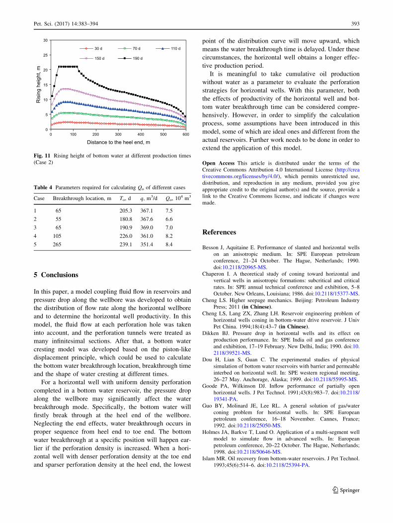
bottom water cresting height of Case 2 is shown in Fig. 11.

It shows that the effect of the perforation density on bottom

water cresting height becomes more serious with the

increase of time. The deformation of the water ridge is

Table 2 Parameters for the

bottom water drive reservoir

and its drilling and completion

parameters

Parameter Value Parameter Value

Reservoir thickness, m 28 Bottom hole pressure, MPa 20

Pressure at the oil–water interface, MPa 25 Horizontal well length, m 600

Horizontal permeability, lm2 0.2 Wellbore diameter, cm 17.45

Vertical permeability, lm2 0.05 Water avoidance height, m 21

Oil density, kg/m3 845 Relative wellbore roughness 0.0001

Oil viscosity, mPa s 15.4 Initial perforation phase angle p/2

Perforation density, shots/m 2 Angle between the wellbore and the x-axis 0

0

0.5

1.0

1.5

2.0

2.5

3.0

3.5

0 100 200 300 400 500 600

Per

fora

tion

dens

ity, s

hots

/m

Distance to the heel end, m

Case 1 Case 2 Case 3

Case 4 Case 5 Case 6

Fig. 4 Cases for variable density perforation

20.0

20.3

20.6

20.9

21.2

21.5

21.8

0 100 200 300 400 500 600

Distance to the heel end, m

Case 1

Case 2

Case 5

Pre

ssur

e, M

Pa

Fig. 5 Pressure distribution along the horizontal wellbore

0

0.002

0.004

0.006

0.008

0

0.01

0.02

0.03

0 100 200 300 400 500 600

Acc

eler

atio

n lo

ss, M

Pa

Fric

tion

loss

, MP

a

Distance to the heel end, m

Friction loss

Acceleration loss

Fig. 6 Friction loss and acceleration loss along the horizontal

wellbore for Case 1

0.30

0.50

0.70

0.90

1.10

0 100 200 300 400 500 600

Flow

rate

, m3 /d

/m

Distance to the heel end, m

Case 1 Case 2 Case 3

Case 4 Case 5 Case 6

Fig. 7 Flow rate distribution along the horizontal wellbore for

different cases

Pet. Sci. (2017) 14:383–394 391

123

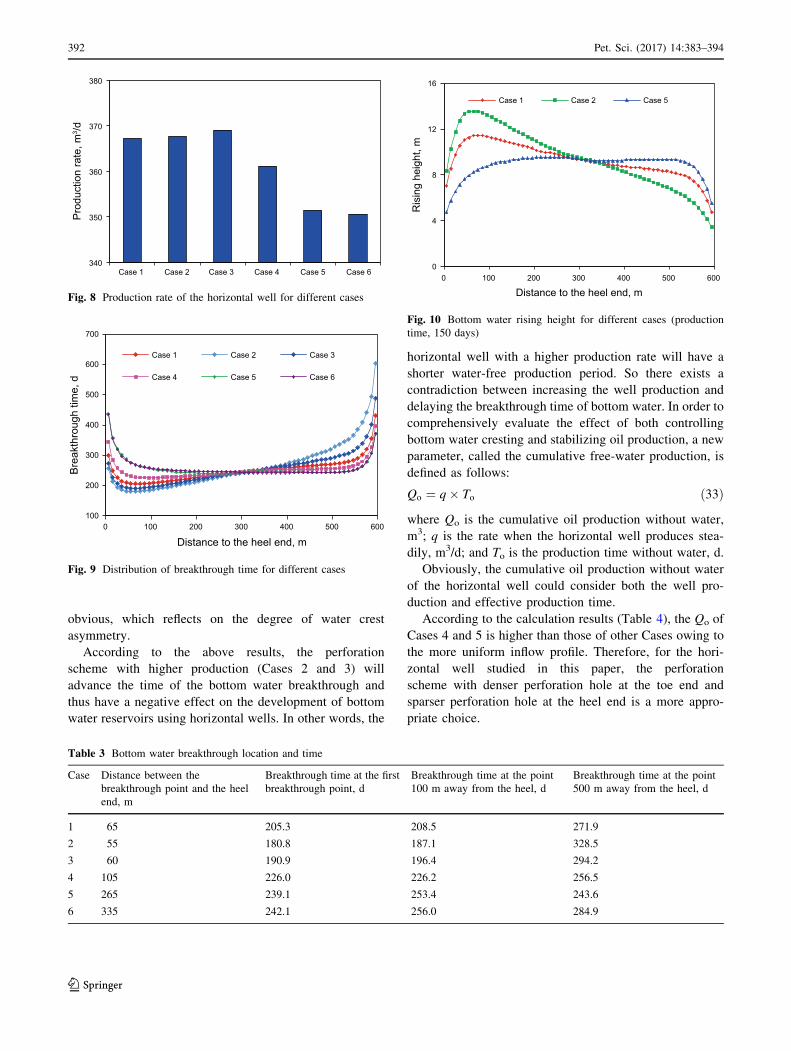
obvious, which reflects on the degree of water crest

asymmetry.

According to the above results, the perforation

scheme with higher production (Cases 2 and 3) will

advance the time of the bottom water breakthrough and

thus have a negative effect on the development of bottom

water reservoirs using horizontal wells. In other words, the

horizontal well with a higher production rate will have a

shorter water-free production period. So there exists a

contradiction between increasing the well production and

delaying the breakthrough time of bottom water. In order to

comprehensively evaluate the effect of both controlling

bottom water cresting and stabilizing oil production, a new

parameter, called the cumulative free-water production, is

defined as follows:

Qo ¼ q� To ð33Þ

where Qo is the cumulative oil production without water,

m3; q is the rate when the horizontal well produces stea-

dily, m3/d; and To is the production time without water, d.

Obviously, the cumulative oil production without water

of the horizontal well could consider both the well pro-

duction and effective production time.

According to the calculation results (Table 4), the Qo of

Cases 4 and 5 is higher than those of other Cases owing to

the more uniform inflow profile. Therefore, for the hori-

zontal well studied in this paper, the perforation

scheme with denser perforation hole at the toe end and

sparser perforation hole at the heel end is a more appro-

priate choice.

340

350

360

370

380P

rodu

ctio

n ra

te, m

3 /d

Case 1 Case 2 Case 3 Case 4 Case 5 Case 6

Fig. 8 Production rate of the horizontal well for different cases

100

200

300

400

500

600

700

0 100 200 300 400 500 600

Bre

akth

roug

h tim

e, d

Distance to the heel end, m

Case 1 Case 2 Case 3

Case 4 Case 5 Case 6

Fig. 9 Distribution of breakthrough time for different cases

Table 3 Bottom water breakthrough location and time

Case Distance between the

breakthrough point and the heel

end, m

Breakthrough time at the first

breakthrough point, d

Breakthrough time at the point

100 m away from the heel, d

Breakthrough time at the point

500 m away from the heel, d

1 65 205.3 208.5 271.9

2 55 180.8 187.1 328.5

3 60 190.9 196.4 294.2

4 105 226.0 226.2 256.5

5 265 239.1 253.4 243.6

6 335 242.1 256.0 284.9

0

4

8

12

16

0 100 200 300 400 500 600

Ris

ing

heig

ht, m

Distance to the heel end, m

Case 1 Case 2 Case 5

Fig. 10 Bottom water rising height for different cases (production

time, 150 days)

392 Pet. Sci. (2017) 14:383–394

123

5 Conclusions

In this paper, a model coupling fluid flow in reservoirs and

pressure drop along the wellbore was developed to obtain

the distribution of flow rate along the horizontal wellbore

and to determine the horizontal well productivity. In this

model, the fluid flow at each perforation hole was taken

into account, and the perforation tunnels were treated as

many infinitesimal sections. After that, a bottom water

cresting model was developed based on the piston-like

displacement principle, which could be used to calculate

the bottom water breakthrough location, breakthrough time

and the shape of water cresting at different times.

For a horizontal well with uniform density perforation

completed in a bottom water reservoir, the pressure drop

along the wellbore may significantly affect the water

breakthrough mode. Specifically, the bottom water will

firstly break through at the heel end of the wellbore.

Neglecting the end effects, water breakthrough occurs in

proper sequence from heel end to toe end. The bottom

water breakthrough at a specific position will happen ear-

lier if the perforation density is increased. When a hori-

zontal well with denser perforation density at the toe end

and sparser perforation density at the heel end, the lowest

point of the distribution curve will move upward, which

means the water breakthrough time is delayed. Under these

circumstances, the horizontal well obtains a longer effec-

tive production period.

It is meaningful to take cumulative oil production

without water as a parameter to evaluate the perforation

strategies for horizontal wells. With this parameter, both

the effects of productivity of the horizontal well and bot-

tom water breakthrough time can be considered compre-

hensively. However, in order to simplify the calculation

process, some assumptions have been introduced in this

model, some of which are ideal ones and different from the

actual reservoirs. Further work needs to be done in order to

extend the application of this model.

Open Access This article is distributed under the terms of the

Creative Commons Attribution 4.0 International License (http://crea

tivecommons.org/licenses/by/4.0/), which permits unrestricted use,

distribution, and reproduction in any medium, provided you give

appropriate credit to the original author(s) and the source, provide a

link to the Creative Commons license, and indicate if changes were

made.

References

Besson J, Aquitaine E. Performance of slanted and horizontal wells

on an anisotropic medium. In: SPE European petroleum

conference, 21–24 October. The Hague, Netherlands; 1990.

doi:10.2118/20965-MS.

Chaperon I. A theoretical study of coning toward horizontal and

vertical wells in anisotropic formations: subcritical and critical

rates. In: SPE annual technical conference and exhibition, 5–8

October. New Orleans, Louisiana; 1986. doi:10.2118/15377-MS.

Cheng LS. Higher seepage mechanics. Beijing: Petroleum Industry

Press; 2011 (in Chinese).Cheng LS, Lang ZX, Zhang LH. Reservoir engineering problem of

horizontal wells coning in bottom-water drive reservoir. J Univ

Pet China. 1994;18(4):43–7 (in Chinese).Dikken BJ. Pressure drop in horizontal wells and its effect on

production performance. In: SPE India oil and gas conference

and exhibition, 17–19 February. New Delhi, India; 1990. doi:10.

2118/39521-MS.

Dou H, Lian S, Guan C. The experimental studies of physical

simulation of bottom water reservoirs with barrier and permeable

interbed on horizontal well. In: SPE western regional meeting,

26–27 May. Anchorage, Alaska; 1999. doi:10.2118/55995-MS.

Goode PA, Wilkinson DJ. Inflow performance of partially open

horizontal wells. J Pet Technol. 1991;43(8):983–7. doi:10.2118/

19341-PA.

Guo BY, Molinard JE, Lee RL. A general solution of gas/water

coning problem for horizontal wells. In: SPE European

petroleum conference, 16–18 November. Cannes, France;

1992. doi:10.2118/25050-MS.

Holmes JA, Barkve T, Lund O. Application of a multi-segment well

model to simulate flow in advanced wells. In: European

petroleum conference, 20–22 October. The Hague, Netherlands;

1998. doi:10.2118/50646-MS.

Islam MR. Oil recovery from bottom-water reservoirs. J Pet Technol.

1993;45(6):514–6. doi:10.2118/25394-PA.

0

5

10

15

20

25

30

0 100 200 300 400 500 600

Ris

ing

heig

ht, m

Distance to the heel end, m

30 d 70 d 110 d

150 d 190 d

Fig. 11 Rising height of bottom water at different production times

(Case 2)

Table 4 Parameters required for calculating Qo of different cases

Case Breakthrough location, m To, d q, m3/d Qo, 104 m3

1 65 205.3 367.1 7.5

2 55 180.8 367.6 6.6

3 65 190.9 369.0 7.0

4 105 226.0 361.0 8.2

5 265 239.1 351.4 8.4

Pet. Sci. (2017) 14:383–394 393

123

Landman MJ, Goldthorpe WH. Optimization of perforation distribu-

tion for horizontal wells. In: SPE Asia-Pacific conference, 4–7

November. Perth, Australia; 1991. doi:10.2118/23005-MS.

Li XG, Wang QH, Li Y. Numerical simulation model of perforated

well completions. J Univ Pet China. 1996;20(2):48–53 (inChinese).

Li GS, Song J, Xiong W, et al. Simulation model and calculation of

seepage flow field for high pressure waterjet perforated wells.

Pet Explor Dev. 2006;32(6):97–100 (in Chinese).Li H, Chen DC, Meng HX. Optimized models of variable density

perforation in the horizontal well. Pet Explor Dev. 2010;37(3):

363–8 (in Chinese).Luo X, Jiang L, Su Y, Huang K. The productivity calculation model

of perforated horizontal well and optimization of inflow profile.

Petroleum. 2015;1(2):154–7. doi:10.1016/j.petlm.2015.04.002.

Muskat M, Wycokoff RD. An approximate theory of water-coning in

oil production. Trans AIME. 2013;114(1):144–63. doi:10.2118/

935144-G.

Novy RA. Pressure drops in horizontal wells: when can they be

ignored. SPE Reserv Eng. 1995;10(1):29–35. doi:10.2118/

24941-PA.

Ouyang LB, Huang B. A comprehensive evaluation of well-comple-

tion impacts on the performance of horizontal and multilateral

wells. In: SPE annual technical conference and exhibition, 9––12

October. Dallas, Texas; 2005. doi:10.2118/96530-MS.

Pang W, Chen DC, Zhang ZP, et al. Segmentally variable density

perforation optimization model for horizontal wells in heteroge-

neous reservoirs. Pet Explor Dev. 2012;39(2):230–8. doi:10.

1016/S1876-3804(12)60036-6.

Penmatcha VR, Arbabi S, Aziz K. A comprehensive reservoir/

wellbore model for horizontal well. In: SPE India oil and gas

conference and exhibition, 17–19 February. New Delhi, India;

1998. doi:10.2118/39521-MS.

Permadi P, Lee RL, Kartoatmodjo RST. Behavior of water cresting

under horizontal wells. In: SPE annual technical conference and

exhibition, 22–25 October. Dallas, Texas; 1995. doi:10.2118/

30743-MS.

Permadi P, Gustiawan E, Abdassah D. Water cresting and oil

recovery by horizontal wells in the presence of impermeable

streaks. In: SPE/DOE improved oil recovery symposium, 21–24

April. Tulsa, Oklahoma; 1996. doi:10.2118/35440-MS.

Sognesand S, Skotner P, Hauge J. Use of partial perforations in

Oseberg horizontal wells. In: SPE annual technical conference

and exhibition, 25–28 September. New Orleans, Louisiana;

1994. doi:10.2118/28569-MS.

Su Z, Gudmundsson JS. Pressure drop in perforated pipes: experi-

ments and analysis. In: SPE Asia Pacific oil and gas conference,

7–10 November. Melbourne, Australia; 1994. doi:10.2118/

28800-MS.

Umnuayponwiwat S, Ozkan E. Water and gas coning toward finite-

conductivity horizontal wells: cone buildup and breakthrough.

In: SPE rocky mountain regional/low-permeability reservoirs

symposium and exhibition, 12–15 March, Denver, Colorado;

2000. doi:10.2118/60308-MS.

Wang RH, Zhang YZ, Bu YH, et al. A segmentally numerical

calculation method for estimating the productivity of perforated

horizontal wells. Pet Explor Dev. 2006;33(5):630–3 (inChinese).

Wibowo W, Permadi P, Mardisewojo P, et al. Behavior of water

cresting and production performance of horizontal well in

bottom water drive reservoir: a scaled model study. In: SPE Asia

Pacific conference on integrated modelling for asset manage-

ment, 29–30 March, Kuala Lumpur, Malaysia; 2004. doi:10.

2118/87046-MS.

Xiong J, He HP, Xiong YM, et al. The effect of partial completion

parameters in horizontal well on water coning. Nat Gas Geosci.

2013;24(6):1232–7 (in Chinese).Yuan H, Sarica C, Brill JP. Effect of perforation density on single

phase liquid flow behavior in horizontal wells. In: SPE

international conference on horizontal well technology, 18–20

November, Calgary, Alberta, Canada; 1996. doi:10.2118/37109-

MS.

Zhao G, Zhou J, Liu X. An insight into the development of bottom

water reservoirs. J Can Pet Technol. 2006;45(4):22–30. doi:10.

2118/06-04-CS.

Zhou ST, Ma DQ, Liu M. Optimization of perforation tunnel

distribution in perforated horizontal wells. J China Univ Pet (Ed

Nat Sci). 2002;26(3):52–4 (in Chinese).

394 Pet. Sci. (2017) 14:383–394

123