References: Bernanke, Ben S. y Alan S. Blinder, (1992), “The Federal Funds Rate and the Channels of Monetary

Transmission”, American Economic Review, vol. 82, nº4, 901-921. Chari, V.V., Patrick J. Kehoe y Ellen R. McGrattan, (2007), “Are Structural VARs with Long-Run

Restrictions Useful in Developing Business Cycle Theory?”, Federal Reserve Bank of Minneapolis, Research Department Staff Report 364. http://www.minneapolisfed.org/research/sr/sr364.pdf See too: Journal of Monetary Economics 55, 1337–52, November 2008.

Christiano, L.J., M. Eichenbaum y C. L. Evans (2005), “ Nominal Rigidities and the Dynamic effects of a Shock to Monetary Policy”, Journal of Political Economy, vol. 113, nº 1, 1-45.

Favero, Carlo A., (2001), Applied Macroeconometrics, Ed. Oxford University Press. Galí, Jordi, (2009), Monetary Policy, Inflation and the Business Cycle. An introduction to the New

Keynesian Framework, Princeton University Press. Hamilton, James, (1994), Time Series Analysis, Ed. Priceton University Press. Ireland, P.N. (2004), “Money’s Role in the Monetary Business Cycle”, Journal of Money, Credit and

Banking, vol. 36, nº 6, 969-983. Leeper, E.M., C. Sims y T. Zha, (1996), “What does Monetary Policy do?”, Brookings Papers on

Economic –Activity, 2, 1-63 Novales, Alfonso, Esther Fernández y Jesús Ruiz, (2009), Economic Growth: Theory and Numerical

Solution Methods, Ed. Springer-Verlag. Walsh, Carl E. (2010), Monetary Theory and Policy, 3nd. ed., The MIT Press.

A New Keynesian Monetary Model The Ireland’s (2004) model

[Ireland, P.N. (2004), “Money’s role in the monetary business cycle”, Journal of Money, credit & Banking, 36(6), 969-983]

Nota: otra versión simple de presentar un modelo monetario neo-keynesiano puede verse en el capítulo 3 del libro Monetary Policy, Inflation, and the Business Cycle, de Jordi Galí, en Princeton University Press, 2008.

1. An Optimizing IS-LM-PC Specification 1.1 Overview

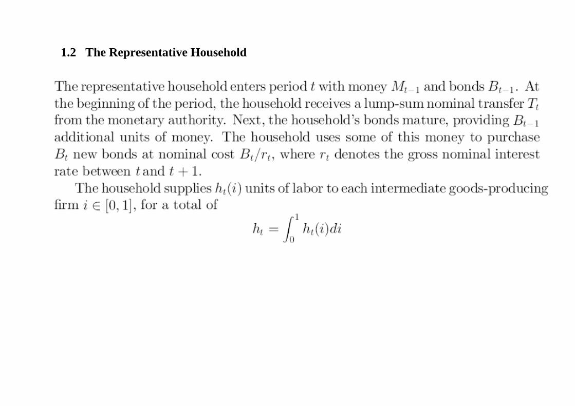
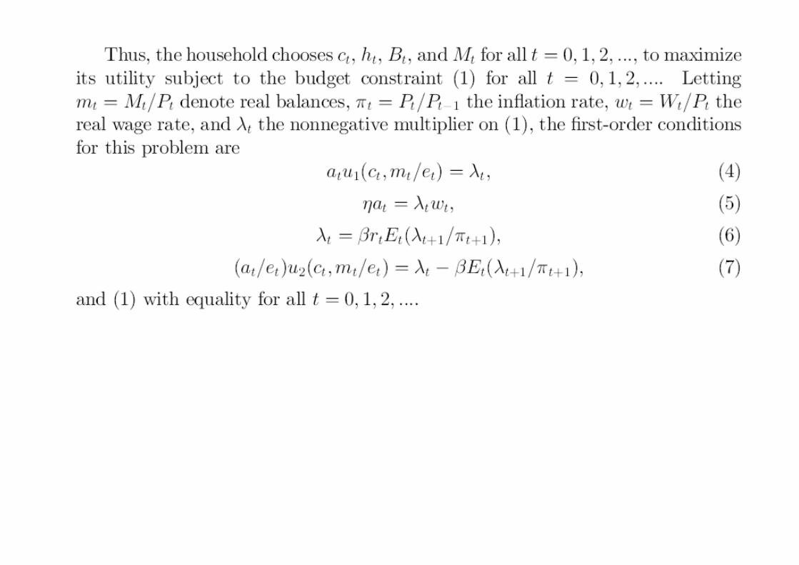
1.2 The Representative Household

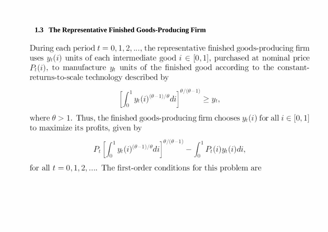
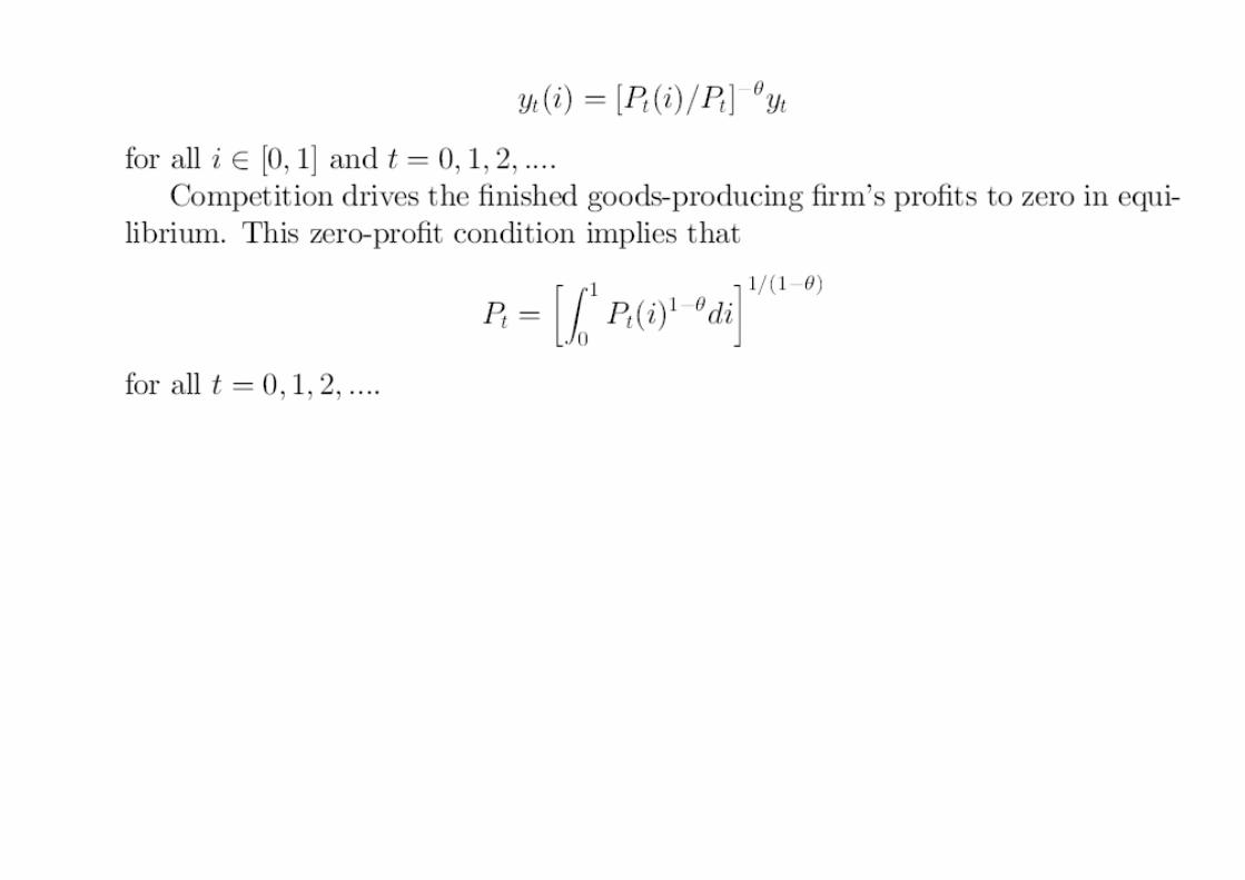
1.3 The Representative Finished Goods-Producing Firm

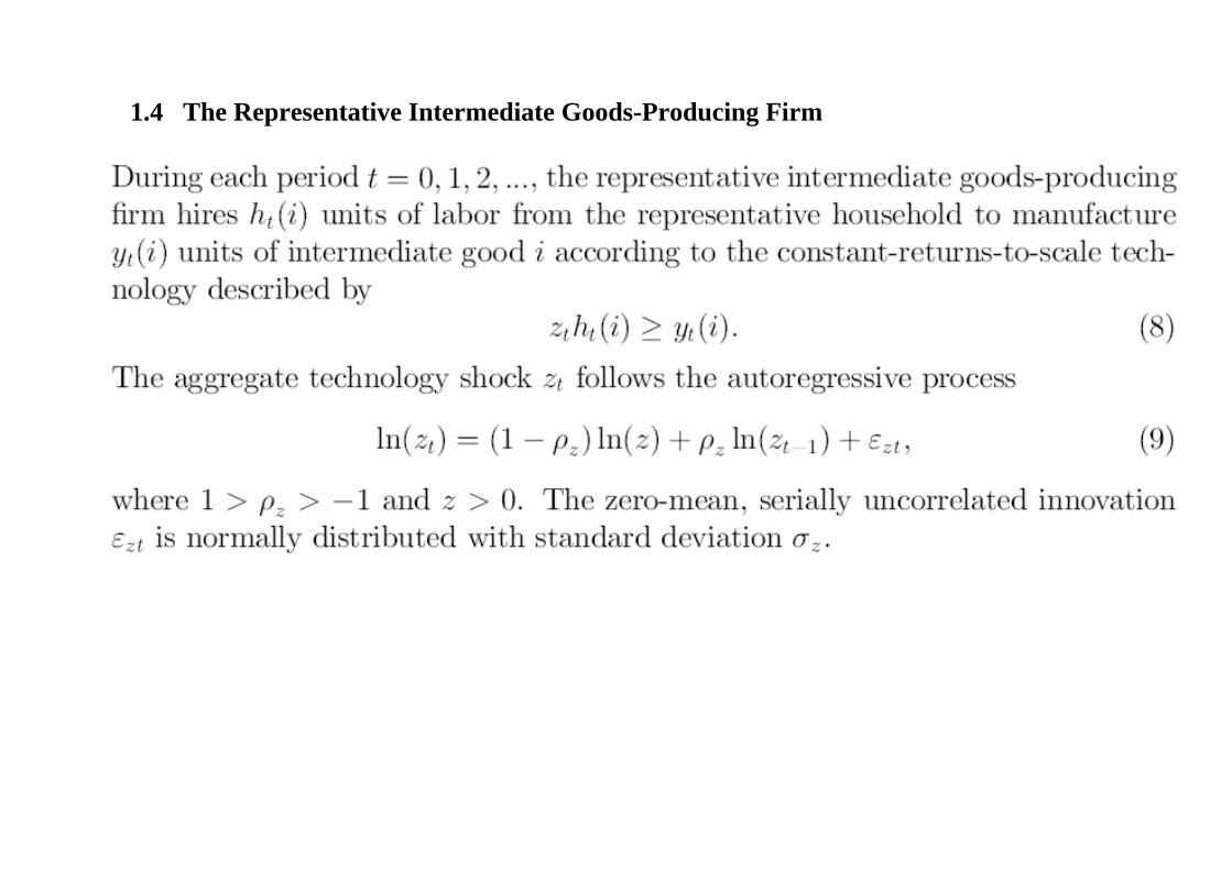
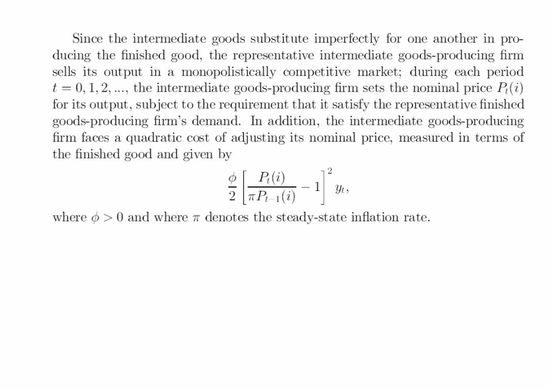
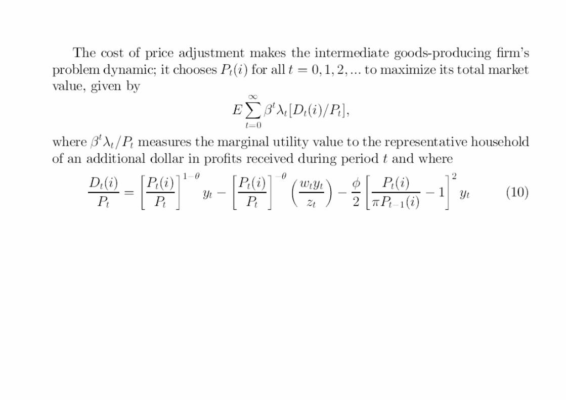
1.4 The Representative Intermediate Goods-Producing Firm

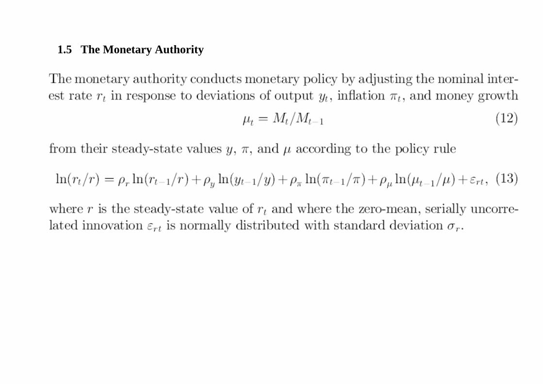
1.5 The Monetary Authority

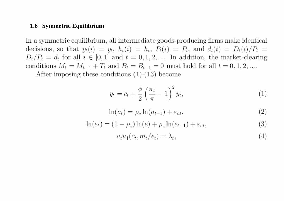
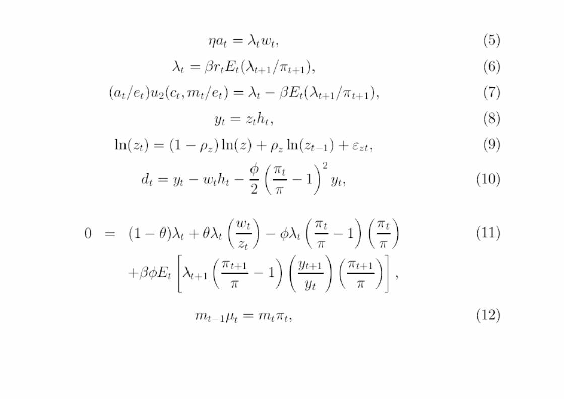
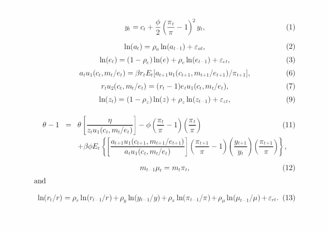
1.6 Symmetric Equilibrium

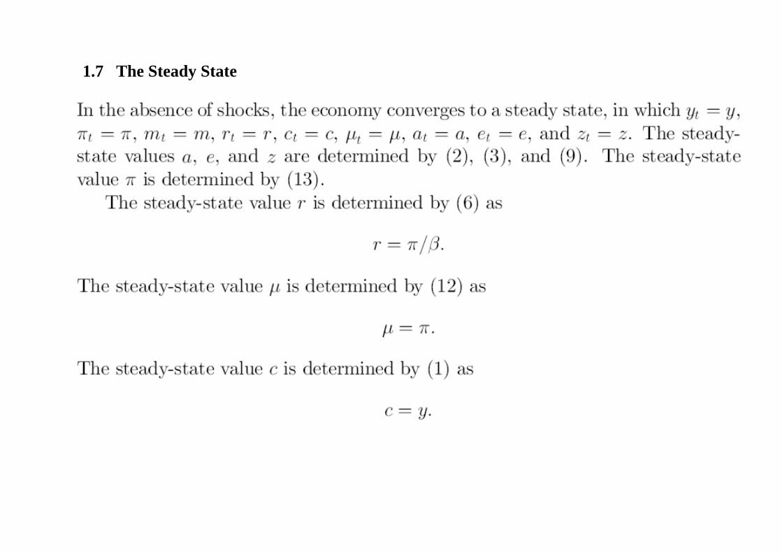
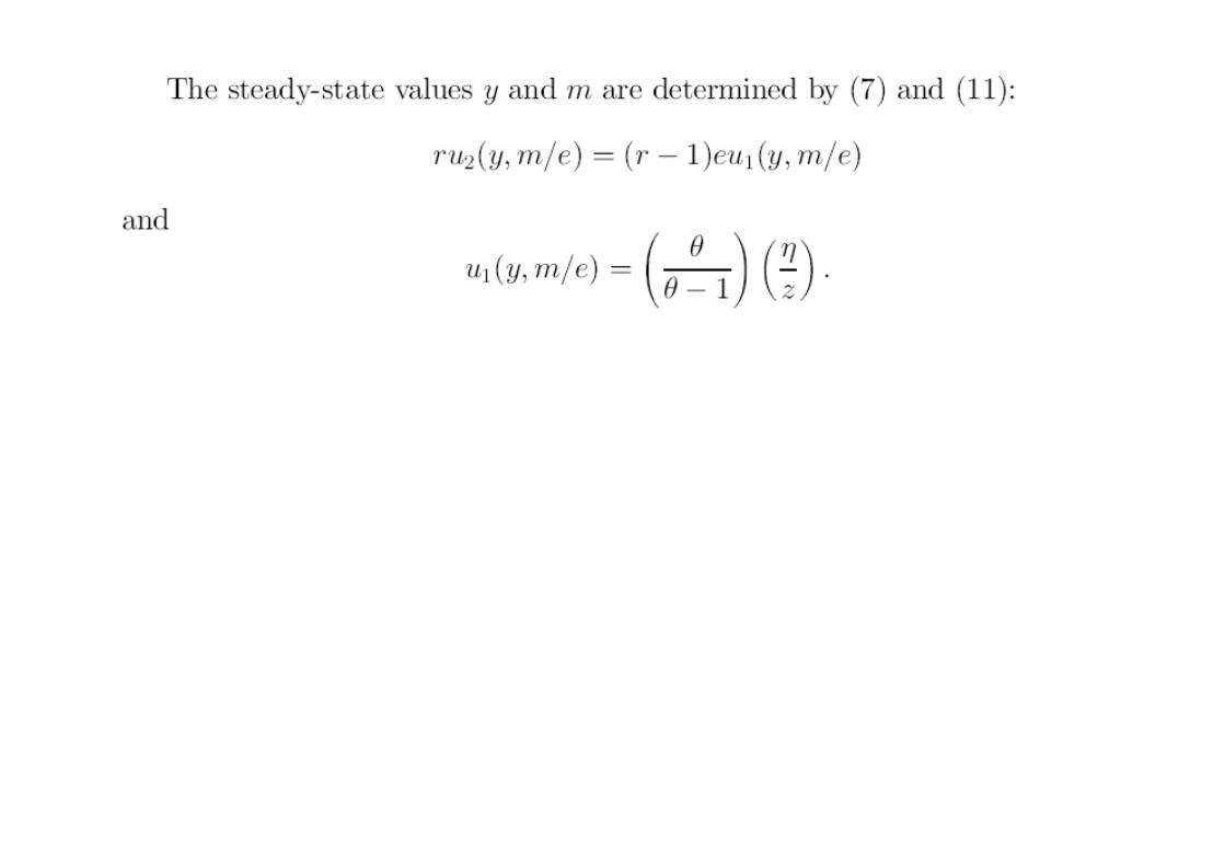
1.7 The Steady State

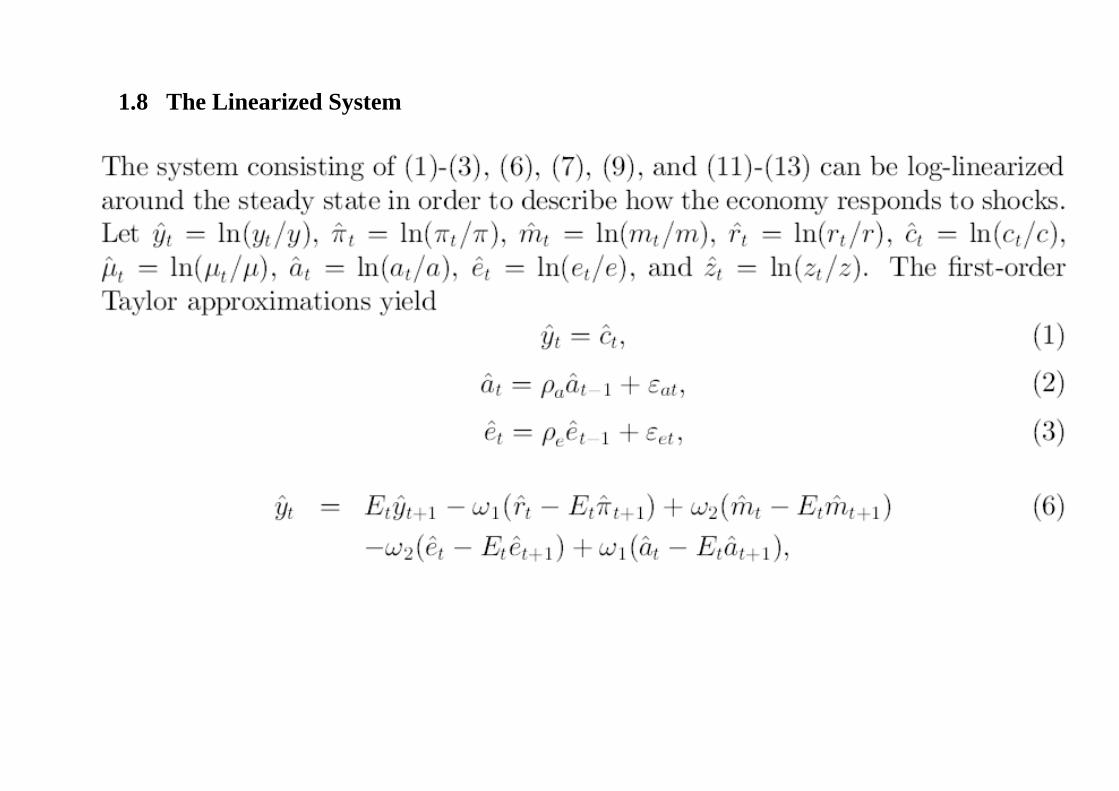
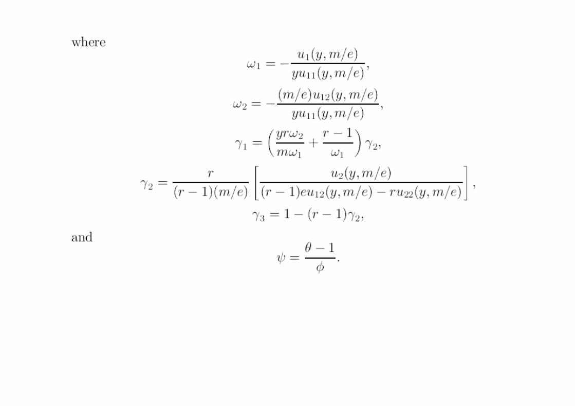
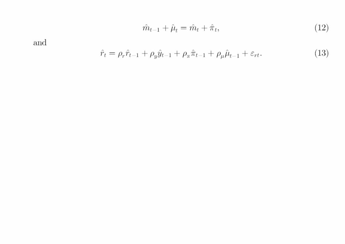
1.8 The Linearized System

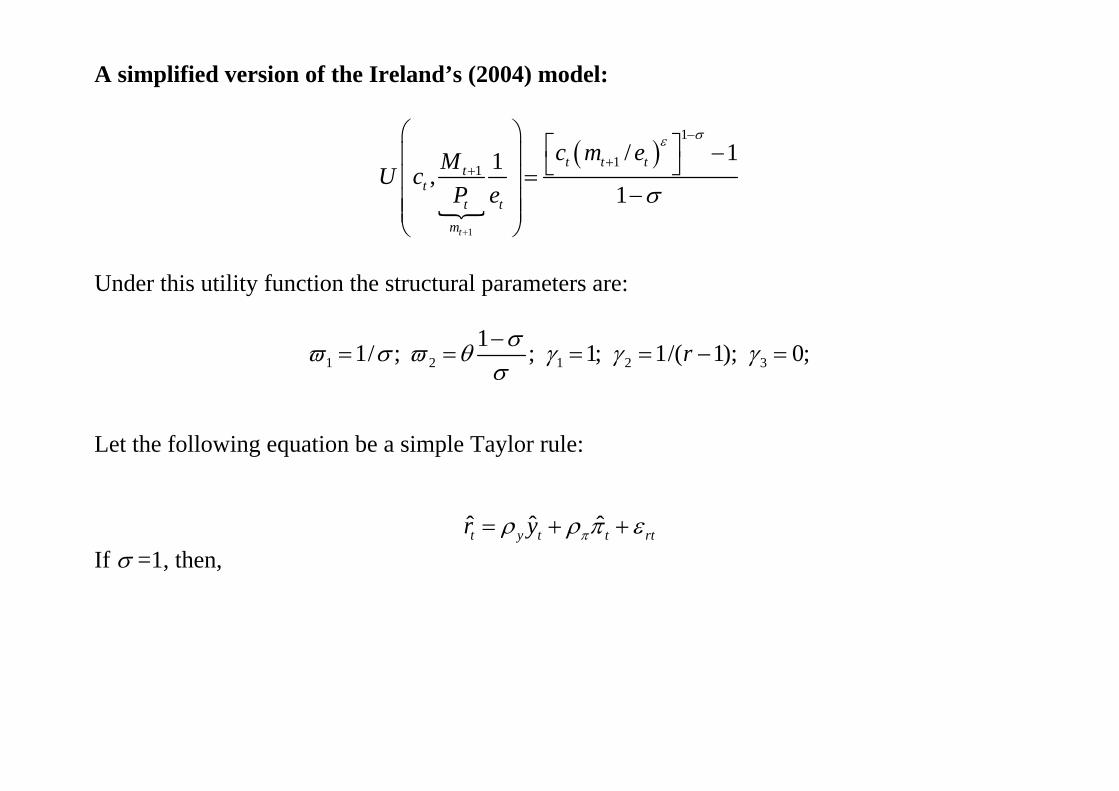
A simplified version of the Ireland’s (2004) model:

1

1

11/ 11,

1t

t t ttt

t t

m

c m eMU cP e

Under this utility function the structural parameters are:

1 2 1 2 311/ ; ; 1; 1/( 1); 0;r

Let the following equation be a simple Taylor rule: ˆ ˆ ˆt y t t rtr y If =1, then,

1

1

1 ˆ ˆ1 11 ˆ ˆ1 0

1 0 1 0 ˆ 1 ˆ0 0 0

ˆ

yt t t

t t t

rta

t

t

t

y E yE

eaz

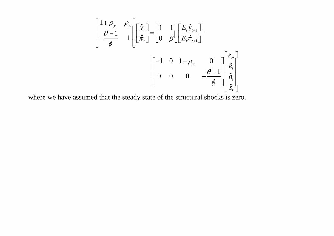
where we have assumed that the steady state of the structural shocks is zero.

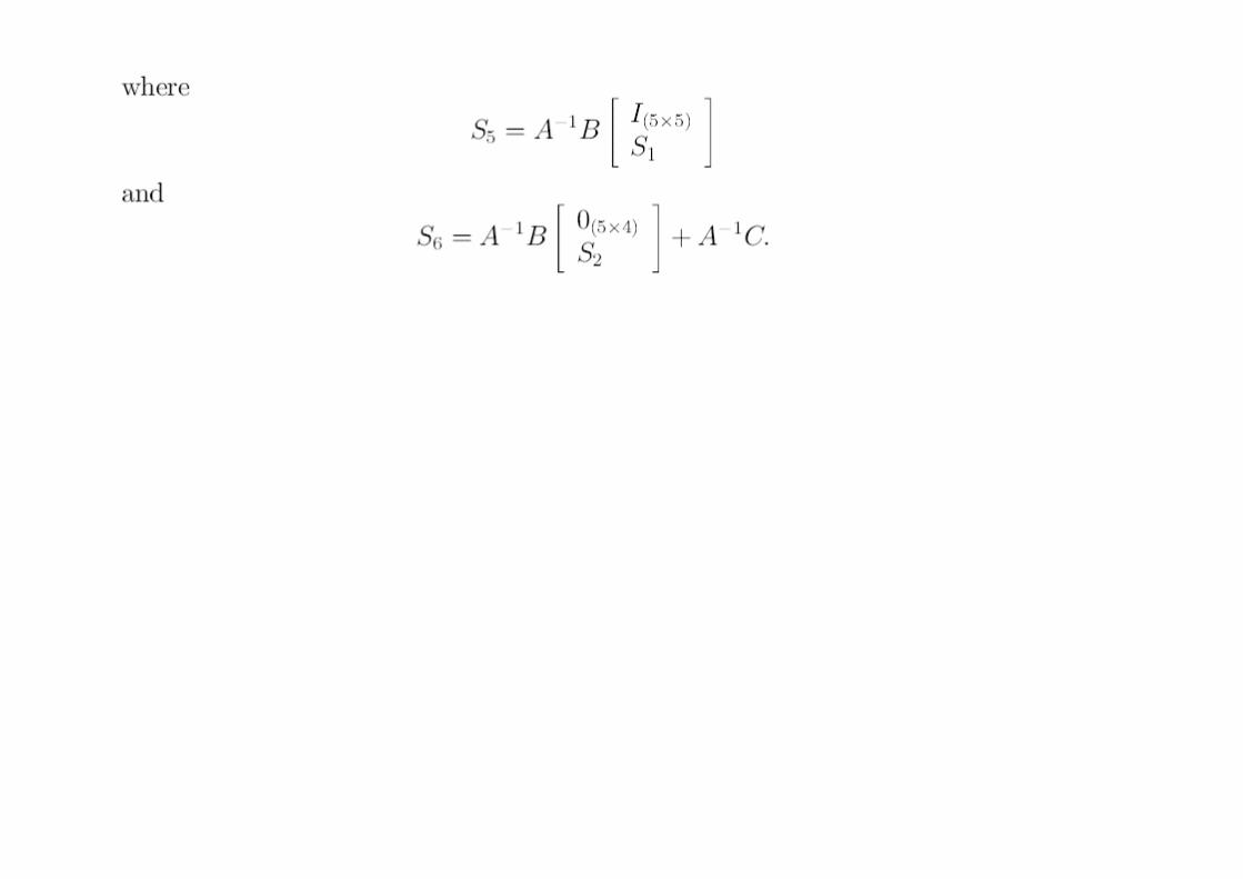
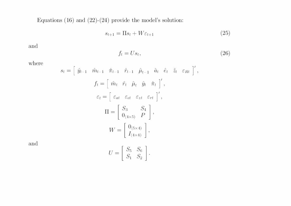
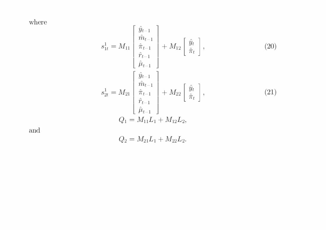
The solution for the system of equations described above is:

1 2 3

1 2 3

2221 11

12 11 111 1 1

12 1222 1121

12

2222 12

122

22 11

12

ˆˆ

ˆˆ

11

where ;1 1

1

1 1

tt

tt

rt

z

z z

z zz zz

z

z

z

a a

zy

a

AC C

A A CA AA A

AA

AC C

AA A

A

11 122 2

12 1221

2223 13

12 11 133 3 3

12 1222 1121

12

1;

1

1 ;

1 1

r

r r

r rr r

r

r

a

a aa

a

A CA A

A

AC C

A A CA AA A

AA

where Aij y Cik are the elements of the following matrices:

1

11 12

21 22

1

11 12 13

21 22 23

11 1

1 1 0

1 0 1 11 11 0 0

y

y a

A AA

A A

C C CC

C C C

Impulse-response functions: Given the following stochastic processes for structural shocks:

1

1

, , 1

ˆ ˆˆ ˆ

r

t z t zt

t z t at

r t r t t

z za a

u

it is easy to derive the impulse-response functions, using the following expressions:

1 , 2 , 30 0 0

1 , 2 , 30 0 0

ˆ

ˆ

r

r

j j jt z z t j a a t j t j

j j j

j j jt z z t j a a t j t j

j j j

y u

u

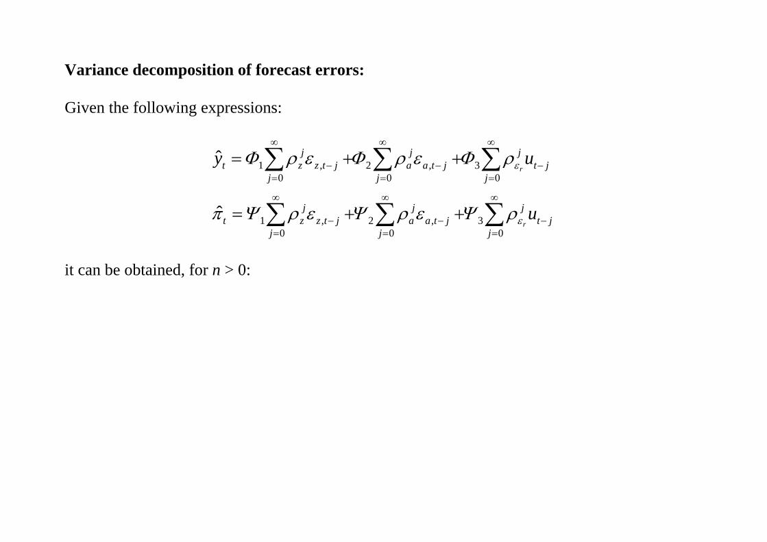
Variance decomposition of forecast errors: Given the following expressions:

1 , 2 , 30 0 0

1 , 2 , 30 0 0

ˆ

ˆ

r

r

j j jt z z t j a a t j t j

j j j

j j jt z z t j a a t j t j

j j j

y u

u

it can be obtained, for n > 0:

1 1 1

1 , 2 , 30 0 0

1 1 1

1 , 2 , 30 0 0

2 22 2 221

2

ˆ ˆ

ˆ ˆ

(1(1 )ˆ ˆ( )

1

r

r

az

n n nj j j

t n t t n z z t n j a a t n j t n jj j j

n n nj j j

t n t t n z z t n j a a t n j t n jj j j

nz

t n t t nz

y E y u

E u

Var y E y

2 2 2 2

32 2

2 2 22 2 2 2 2 221 3

1 2 2 2

212

20

) (1 )1 1

(1 )(1 ) (1 )ˆ ˆ( )

1 1 1

(1 )Note that: .1

r

r

az r

r

n na u

a

nn naz u

t t t nz a

nn

j

Var E

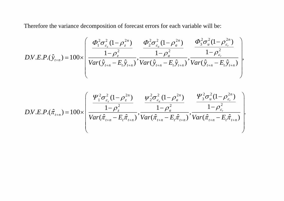
Therefore the variance decomposition of forecast errors for each variable will be:

2 2 22 2 22 2 2321

222

2 2 21

2

(1 )(1 )(1 )111ˆ. . . .( ) 100 , , ,

ˆ ˆ ˆ ˆ ˆ ˆ( ) ( ) ( )

(1 )1ˆ. . . .( ) 100ˆ(

raz

r

z

nnnuaz

azt n

t n t t n t n t t n t n t t n

nz

zt n

t

DV E P yVar y E y Var y E y Var y E y

DV E PVar

2 2 22 2 232

22

(1 )(1 )11, , .

ˆ ˆ ˆ ˆ ˆ) ( ) ( )

ra

r

nnua

a

n t t n t n t t n t n t t nE Var E Var E

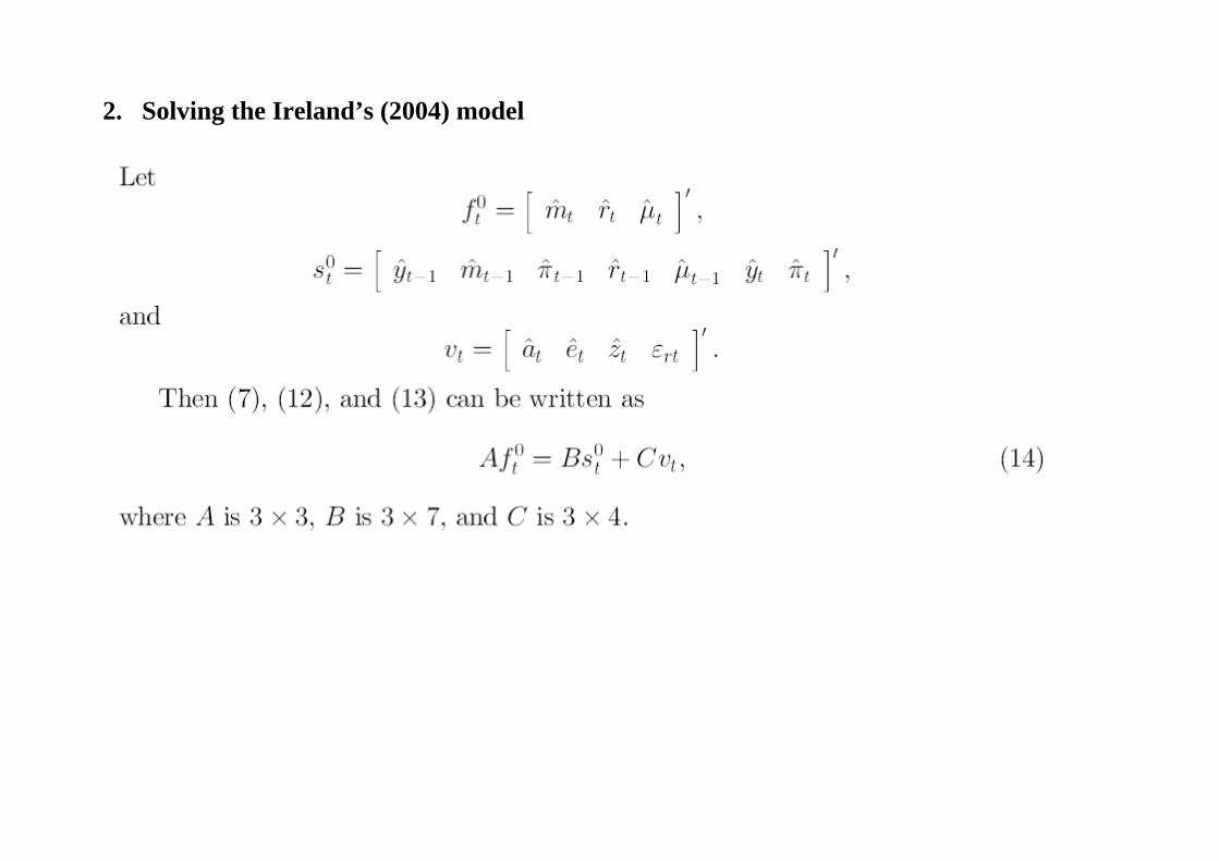
2. Solving the Ireland’s (2004) model

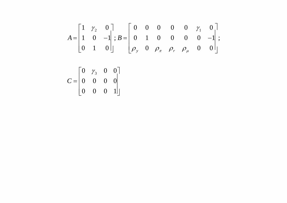
2 1

3

1 0 0 0 0 0 0 01 0 1 ; 0 1 0 0 0 0 1 ;0 1 0 0 0 0

0 0 00 0 0 00 0 0 1

y r

A B

C

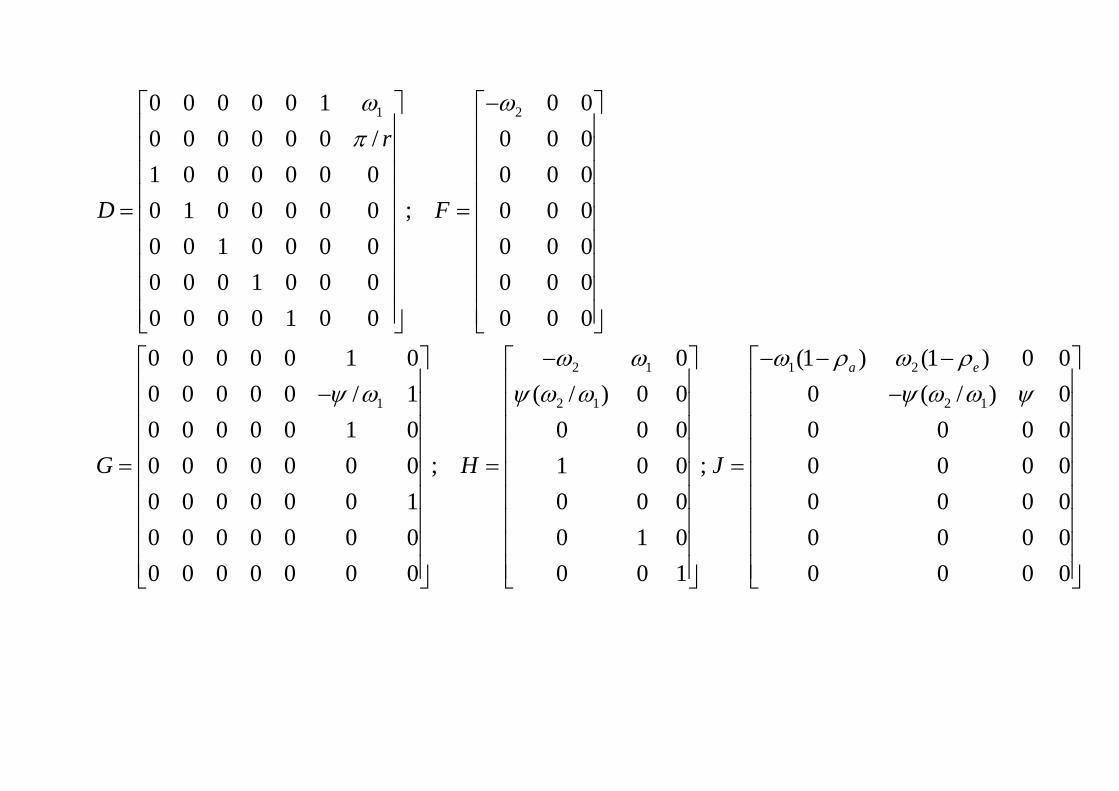
1 2

1

0 0 0 0 0 1 0 00 0 0 0 0 0 / 0 0 01 0 0 0 0 0 0 0 0 0

;0 1 0 0 0 0 0 0 0 00 0 1 0 0 0 0 0 0 00 0 0 1 0 0 0 0 0 00 0 0 0 1 0 0 0 0 0

0 0 0 0 0 1 00 0 0 0 0 / 10 0 0 0 0 1 00 0 0 0 0 0 00 0 0 0 0 0 10 0 0 0 0 0 00 0 0 0 0 0 0

r

D F

G

2 1 1 2

2 1 2 1

0 (1 ) (1 ) 0 0( / ) 0 0 0 ( / ) 0

0 0 0 0 0 0 0; ;1 0 0 0 0 0 0

0 0 0 0 0 0 00 1 0 0 0 0 00 0 1 0 0 0 0

a e

H J

Blanchard, O. and C.M. Kahn (1980), “The solution of linear difference models under rational expectations”, Econometrica, 48(5), 1305-1311.

11

(8 8) 2 2( )I P N vec Q