A New Keynesian Model with Robots: Implications for...
38
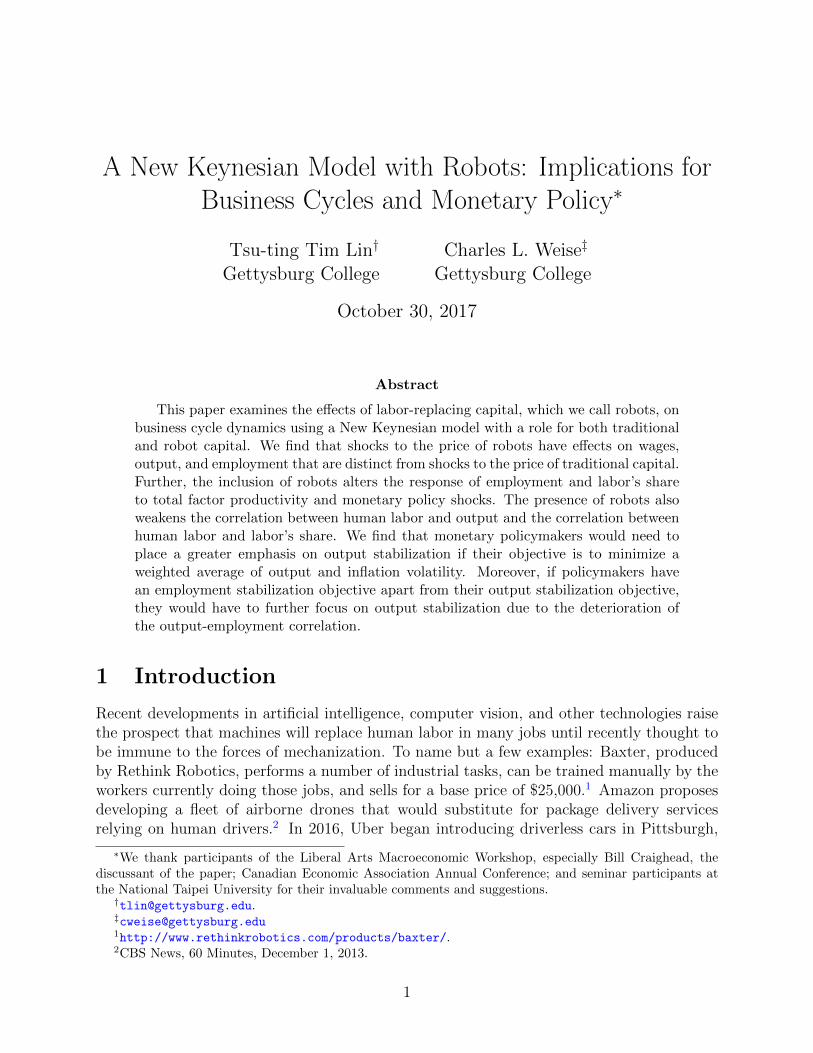
A New Keynesian Model with Robots: Implications for Business Cycles and Monetary Policy * Tsu-ting Tim Lin † Gettysburg College Charles L. Weise ‡ Gettysburg College October 30, 2017 Abstract This paper examines the effects of labor-replacing capital, which we call robots, on business cycle dynamics using a New Keynesian model with a role for both traditional and robot capital. We find that shocks to the price of robots have effects on wages, output, and employment that are distinct from shocks to the price of traditional capital. Further, the inclusion of robots alters the response of employment and labor’s share to total factor productivity and monetary policy shocks. The presence of robots also weakens the correlation between human labor and output and the correlation between human labor and labor’s share. We find that monetary policymakers would need to place a greater emphasis on output stabilization if their objective is to minimize a weighted average of output and inflation volatility. Moreover, if policymakers have an employment stabilization objective apart from their output stabilization objective, they would have to further focus on output stabilization due to the deterioration of the output-employment correlation. 1 Introduction Recent developments in artificial intelligence, computer vision, and other technologies raise the prospect that machines will replace human labor in many jobs until recently thought to be immune to the forces of mechanization. To name but a few examples: Baxter, produced by Rethink Robotics, performs a number of industrial tasks, can be trained manually by the workers currently doing those jobs, and sells for a base price of $25,000. 1 Amazon proposes developing a fleet of airborne drones that would substitute for package delivery services relying on human drivers. 2 In 2016, Uber began introducing driverless cars in Pittsburgh, * We thank participants of the Liberal Arts Macroeconomic Workshop, especially Bill Craighead, the discussant of the paper; Canadian Economic Association Annual Conference; and seminar participants at the National Taipei University for their invaluable comments and suggestions. † [email protected]. ‡ [email protected] 1 http://www.rethinkrobotics.com/products/baxter/. 2 CBS News, 60 Minutes, December 1, 2013. 1
Transcript of A New Keynesian Model with Robots: Implications for...
A New Keynesian Model with Robots: Implications forBusiness Cycles and Monetary Policy∗
Tsu-ting Tim Lin†
Gettysburg CollegeCharles L. Weise‡
Gettysburg College
October 30, 2017
Abstract
This paper examines the effects of labor-replacing capital, which we call robots, onbusiness cycle dynamics using a New Keynesian model with a role for both traditionaland robot capital. We find that shocks to the price of robots have effects on wages,output, and employment that are distinct from shocks to the price of traditional capital.Further, the inclusion of robots alters the response of employment and labor’s shareto total factor productivity and monetary policy shocks. The presence of robots alsoweakens the correlation between human labor and output and the correlation betweenhuman labor and labor’s share. We find that monetary policymakers would need toplace a greater emphasis on output stabilization if their objective is to minimize aweighted average of output and inflation volatility. Moreover, if policymakers havean employment stabilization objective apart from their output stabilization objective,they would have to further focus on output stabilization due to the deterioration ofthe output-employment correlation.
1 Introduction
Recent developments in artificial intelligence, computer vision, and other technologies raisethe prospect that machines will replace human labor in many jobs until recently thought tobe immune to the forces of mechanization. To name but a few examples: Baxter, producedby Rethink Robotics, performs a number of industrial tasks, can be trained manually by theworkers currently doing those jobs, and sells for a base price of $25,000.1 Amazon proposesdeveloping a fleet of airborne drones that would substitute for package delivery servicesrelying on human drivers.2 In 2016, Uber began introducing driverless cars in Pittsburgh,
∗We thank participants of the Liberal Arts Macroeconomic Workshop, especially Bill Craighead, thediscussant of the paper; Canadian Economic Association Annual Conference; and seminar participants atthe National Taipei University for their invaluable comments and suggestions.†[email protected].‡[email protected]://www.rethinkrobotics.com/products/baxter/.2CBS News, 60 Minutes, December 1, 2013.
1
Pennsylvania, with the ultimate goal of replacing the more than one million human Uberdrivers.3 Software that grades student essays—a task that is a core function of high schooland university-level teaching—is now produced commercially by at least nine companies.4
New technological advances and declining costs raise the prospect of a “Cambrian Explosion”in robotics that could accelerate this trend (Pratt (2015)).
A number of recent commentators have warned that the latest round of automationhas had an adverse impact on wages and employment, and that the situation will only getworse. Brynjolfsson and McAfee (2014) link the stagnation of median wages and labor’sdeclining share of income since the 1980’s to automation. In a blog post provocativelyentitled “Rise of the Robots,” Krugman (2012) projected that mechanization is likely tocontinue to reduce labor’s share of income in the future. Summers (2013) confesses that heis not now as confident as he was as a student that “the Luddites were wrong and the believersin technology and technological progress were right.” Perhaps the starkest expression of thenightmare scenario is the prediction of Leontief (1983) that “the role of humans as the mostimportant factor of production is bound to diminish in the same way that the role of horsesin agricultural production was first diminished and then eliminated by the introduction oftractors.”
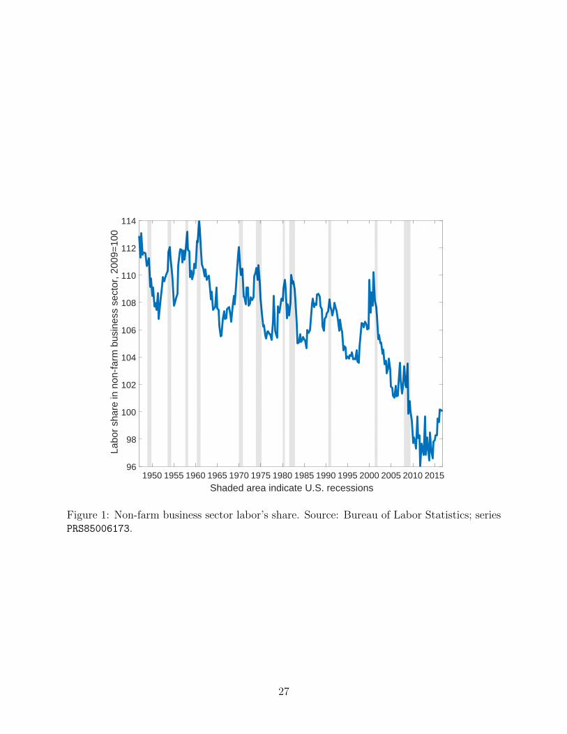
The long-run effects of robotization on wages and employment have been examined in anumber of recent papers.5 The effect of robotization at business cycle frequencies, however,has not been studied. These effects are potentially important. Casual inspection of Figure1 shows that labor’s share fluctuates over the business cycle. Up to the 1990s, the typicalpattern was for labor’s share to fall during the recession and in the early stages of recovery,then rise during the recovery and expansion period. In the last two business cycles, however,labor’s share has fallen particularly strongly during the recession and early recovery periodand failed to climb during the expansion. This pattern is consistent with robotization playinga greater role during recessions and expansions than in earlier business cycles.
This paper is the first of which we are aware to examine the effects of robotization atbusiness cycle frequencies. We incorporate robot capital into a medium-sized New Keynesianmodel along the lines of Smets and Wouters (2005). We use the model to address a numberof issues: how does the presence of robot capital affect the economy’s response to total factorproductivity shocks and monetary policy shocks; how do shocks to the price of robot capitalaffect the economy, and how are these effects different from the effects of traditional capitalprice shocks; can the presence of robot capital help explain the behavior of labor’s share ofincome over the business cycle; to what extent does the presence of robots affect monetarypolicy?
Section 2 of this paper gives an overview of the literature on the effects of robotization.Section 3 introduces the model used in our analysis. Section 4 discusses the results of themodel, including the long-run effect of permanent changes to the cost of robot capital; theeffect of shocks at the business cycle frequency; the effect of robots on the correlation oflabor’s share and output; and the implications for monetary policy. Section 5 concludes.
3Bloomberg, August 18, 2016. https://www.bloomberg.com/news/features/2016-08-18/
uber-s-first-self-driving-fleet-arrives-in-pittsburgh-this-month-is06r7on.4Shermis and Hamner (2013)5We will provide a brief overview of the literature in section 2.
2
2 Effect of Robots
How does a robot differ from traditional capital? A simplistic distinction is that robotssubstitute for human labor whereas traditional capital complements it. But many types ofcapital that we do not associate with robots displace human labor: power looms displacedhand weavers in the early stages of the industrial revolution; a chainsaw or a backhoe reducesthe number of workers required to chop down a tree or lay the foundation for a new house.The introduction of any machine replaces labor in the task to which it is applied.
The distinction between traditional capital and robots may be more clear at the firm orindustry level. Acemoglu and Autor (2011), propose a production function in which outputis produced by a number of tasks. Each task requires certain skills that may be possessed byhuman laborers and/or physical capital (machines). Technological change or the introductionof a new type of machine give machines a comparative advantage in certain tasks that hadbeen carried out by human labor, resulting in a substitution of machines for human labor atparticular stages in the production process. On the other hand, those same machines mayincrease the productivity of human workers employed in other tasks, causing a reallocationof workers towards those tasks. This direct effect on employment in a particular industrydepends on the number of workers displaced by machinery relative to the number drawn into complementary tasks. The new technologies discussed above may be of a type or of amagnitude such that they displace human labor within the firm or industry at a faster pacethan they increase demand for complementary tasks.
However, even when robotization displaces human labor at the industry level, the gen-eral equilibrium effects may offset this reduction in human labor. There are at least threepotential mitigating factors.
First, the introduction of new machinery increases the marginal product of complemen-tary types of physical capital. This induces investment in traditional capital, which is com-plementary to human labor and therefore tends to increase employment or wages or both.For example, the arrival of online retail on a massive scale in the 1990s displaced many work-ers. At the same time, online retail required investment in warehousing and transportationnetworks which increased demand for labor in those sectors.
Second, robots require human labor in their production. Introduction of robots mayreplace workers in one sector—e.g., on auto assembly lines—but increase the demand forworkers in the robot production industry. To the extent that robot investment brings withit more investment in structures and other equipment, human labor may be required in theproduction of those items as well.
Finally, the employment effects of the introduction of labor-displacing machinery willdepend on the extent to which greater productivity is matched by an increase in aggregatedemand. An increase in aggregate demand following an influx of robots will facilitate themovement of labor to other sectors of the economy, whereas if aggregate demand is notresponsive aggregate employment and wages may fall.
The direct and the mitigating factors of new technologies on employment and wagesin the long run have been studied extensively. Autor (2015) is skeptical that automationwill result in fewer jobs, emphasizing the complementarity between machines and humansdoing particular tasks within a firm or industry. Bessen (2015), for example, finds that bankteller employment actually increased following the introduction of ATMs as bank tellers
3

were reassigned from cash-handling tasks to “relationship banking” tasks. Acemoglu andRestrepo (2016) develop a model in which the effects of automation on labor demand aredetermined by the interplay of automation that substitutes for human labor in certain tasks,the creation of new tasks for human labor, the effect of automation on the productivity oflabor in tasks related to those being automated, and investment in new capital stimulatedby productivity-enhancing automation. In their model, wages always increase in the longrun following an increase in automation though labor’s share of income falls.
These considerations are as relevant to the short-run effects of robots—the primary focusof this paper—as they are to the long-run effects examined in previous research. We explorethree types of issues in this paper.
First, we explore how investment specific shocks that lower the price of robot capital differin their economic effects from shocks to total factor productivity (TFP) or to the price oftraditional capital investment. The key distinction is that whereas TFP shocks or a decreasein the cost of traditional capital resulting in an increase in investment has the direct effect ofincreasing the marginal product of labor and hence increasing labor demand, a decrease inthe cost of robot capital that causes increased investment in robot capital may subsequentlycrowd out human labor. We are interested in the implications for wages, employment, andlabor’s share of income.
Second, it has been noted—e.g., by Boldrin and Horvath (1995) and Choi and Rıos-Rull (2009)—that labor’s share of income varies over the business cycle. Specifically, theseauthors find that labor’s share is negatively correlated with output contemporaneously, butthat output is positively correlated with leads of labor’s share. Choi and Rıos-Rull (2009)refers to this as an “overshooting” effect: increases in output due for example to shocks toTFP reduce labor’s share on impact but increase it over time. The authors find that neitherthe standard real business cycle model nor modifications involving search rigidities in labormarkets are able to replicate this phenomenon. They suggest that incorporating a constantelasticity of substitution (CES) rather than Cobb-Douglas production function in the modelmay account for the cyclical behavior of labor share. In this paper we examine the behaviorof labor’s share in the presence of robot capital using a similar CES production function.
Lastly, we are interested in the implications of the presence of robot capital for theconduct of monetary policy. The presence of robots alters the relationship between outputand employment over the business cycle. The effect of robot investment on wages has aneffect on current and expected future marginal cost, thereby altering the cyclical behaviorof inflation as well. We leave a formal analysis of optimal monetary policy in this model forfuture research, but identify the general effects of robots on the emphasis a monetary policyauthority would place on output and inflation stabilization objectives in its monetary policyrule if its objective is to minimize a weighted average of output and inflation volatilities.
We explore these issues in a model calibrated to match the current importance of robotcapital in the U.S. economy. Given the current trends in technology, however, we are alsointerested in the answers to the questions posed above in a model in which robot capitalplays a considerably larger role than it does today.
4
3 Model
Our model builds upon Smets and Wouters (2005) by incorporating robots via a nested CESproduction function. The model consists of a representative final good firm, a continuumof intermediate good firms, a continuum of labor unions, a representative household, and amonetary authority. The final good firm produces output using intermediate goods. Inter-mediate goods firms produce intermediate goods using capital, robots, and an aggregate ofdifferentiated labor supplied by labor unions. Intermediate goods prices and wages are set bymonopolistically competitive firms and labor unions respectively under Calvo (1983) pricing.The household owns the firms, purchases consumption goods, and places its savings in theform of bonds, traditional capital, and robots. The household also supplies undifferentiatedhuman labor to the labor unions which transform it into differentiated labor which is hiredby the intermediate good firms.
We begin our discussion of the model with the final good producers.
3.1 Production
3.1.1 Final Good Firms
Competitive final good producers purchase differentiated intermediate goods from interme-diate goods producers to produce a composite final good. The production of a final good ytuses intermediate goods yt(i), i ∈ [0, 1], using the production function:
yt =
(∫ 1
0
yt(i)1εy di
)εy,
where εy > 1. Profit maximization and perfect competition imply the demand for interme-diate good i is
yt(i) =
(Pt(i)
Pt
) εy1−εy
yt,
where the final good price index is
Pt =
(∫ 1
0
Pt(i)1
1−εy di
)1−εy
.
3.1.2 Intermediate Good Firms
There is a continuum of intermediate good firms owned by the representative household.They are indexed by i ∈ [0, 1]. Each period a fraction (1 − λy) ∈ [0, 1] of the intermediategood firms can re-optimize its price. The remainder sets price according to the indexationrule:
Pt(i) = πt−1ηyPt−1(i),
5

where πt−1 = Pt−1
Pt−2is the gross inflation rate in the economy, and ηy is the inflation index-
ation parameter. The intermediate good producer i has access to a constant elasticity ofsubstitution production technology:
yt(i) = zt
[θkkt(i)
α+ (1− θk)`t(i)α
] 1α,
where zt is total factor productivity, kt is utilization-adjusted traditional capital, and `t iscomposite labor input. `t is an aggregation of utilization-adjusted robots at and human laborinput nt:
`t(i) =[θaat(i)
φ + (1− θa)nt(i)φ] 1φ.
Our use of the CES production function rather than the traditional Cobb-Douglas func-tion enables us to distinguish between traditional capital, which complements human laborat the level of the industry, and robot capital, which substitutes for human labor. Thecurvature parameters α and φ determine the degree of substitutability or complementaritybetween the two forms of capital and human labor. The elasticity of substitution betweentraditional capital and composite labor is 1
1−α while the elasticity of substitution between
composite and human labor is 11−φ . Below we will maintain the assumption that α < 0,
implying that the elasticity of substitution between traditional capital and composite laboris less than one, hence traditional capital and composite labor are gross complements. Wewill assume that φ > 0, implying that the elasticity of substitution between robot capital andhuman labor is greater than one, hence robot capital and human labor are gross substitutes.
The intermediate good firms rent capital and robots from the households and hire laborinput from labor unions. Total factor productivity zt follows the stochastic processes:
ln zt = ρz ln zt−1 + ςzηzt , ηzt ∼ i.i.d. N (0, 1).
Intermediate good firm i’s cost minimization problem is:
min{kt(i),at(i),nt(i)}
Ptrkt kt(i) + Ptr
at at(i) +Wtnt(i),
subject to production technology:
yt(i) = zt
{θkkt(i)
α+ (1− θk)
[θaat(i)
φ + (1− θa)nt(i)φ]αφ
} 1α
,
where rkt , rat , and Wt are the capital rental rate, robot rental rate, and nominal wage which
firms take as given. It can be shown that, taking factor prices and productivity as given, eachintermediate good firm’s cost-minimization problem implies the marginal cost of productionis constant with respect to the level of output and is independent of i. Since marginal costis identical across firms, we can drop the i subscript in the price adjustment problem below.
Each price re-optimizing firm chooses price Pt to maximize its expected profit. Since theintermediate good firms are owned by the household, they discount future profits using the
6
household’s stochastic discount factor. We can express a price-adjusting intermediate goodfirm’s price-setting problem as:
maxPt
Et∞∑s=0
(βλy)s Λt+s
Pt+s
(Pt
s∏k=1
πt−1+kηy −MCt+s
)yt+s,
where Λt+s is the household’s marginal utility; MCt+s is the marginal cost of production;and yt+s is the period t+ s demand for an optimizing firm’s output, assuming its last priceadjustment was in period t.
3.2 Household
The representative household owns the stock of physical capital kt and robots at and makesinvestment decisions ikt and iat . The household chooses the levels of utilization for capital androbots µkt and µat which incur utilization costs Ψk(µ
kt ) and Ψa(µ
at ). The household purchases
nominal bonds Dt and receives dividend payments Divt+s from its ownership of intermediategood producers.
The household’s lifetime utility is:
Et∞∑s=0
βs
[(ct+s − hct−1+s)1−γ
1− γ− κn
nt+s1+σ
1 + σ
].
Its budget constraint is:
ct+s +Dt+s
Pt+s+ ikt+s + iat+s + Ψk
(µkt+s
)kt+s + Ψa
(µat+s
)at+s ≤
Wt+s
Pt+snt+s + rkt+sµ
kt+skt+s + rkt+sµ
at+sat+s +Rt−1+s
Dt−1+s
Pt+s+Divt+sPt+s
.
Here β is the discount factor; ct+s is the level of consumption; h captures habit formation;γ is the coefficient of relative risk aversion; κn and σ capture the disutility of work.
In addition to the variables already described above, rkt+s and rat+s are the rental ratesfor each unit of effective capital µkt+skt+s and effective robot µat+sat+s, respectively. Thehouseholds earn gross interest Rt+s for each unit of nominal bonds they hold.
The capital and robot laws of motion are:
kt+1+s = (1− δk)kt+s + εkt+s
[1− Sk
(ikt+sikt−1+s
)]ikt+s;
at+1+s = (1− δa)at+s + εat+s
[1− Sa
(iat+siat−1+s
)]iat+s,
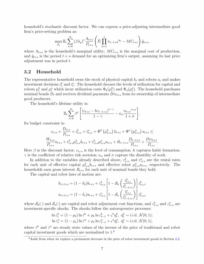
where Sk(·) and Sa(·) are capital and robot adjustment cost functions, and εkt+s and εat+s areinvestment-specific shocks. The shocks follow the autoregressive processes:
ln εkt = (1− ρk) ln εk + ρk ln εkt−1 + ςkηkt , ηkt ∼ i.i.d. N (0, 1);
ln εat = (1− ρa) ln εa + ρa ln εat−1 + ςaηat , ηat ∼ i.i.d. N (0, 1),
where εk and εa are steady state values of the inverse of the price of traditional and robotcapital investment goods which are normalized to 1.6
6Aside from when we explore a permanent decrease in the price of robot investment goods in Section 4.2.
7

The specifications for the utilization cost and investment adjustment cost functions arestandard and are specified in Appendix A.
3.3 Labor Unions
There is a unit measure of labor unions indexed by j ∈ [0, 1]. The representative householdsupplies undifferentiated labor to labor unions, which in turn supply type j labor nt(j).Differentiated labor is then combined using:
nt+s =
(∫ 1
0
nt+s(j)1εn dj
)εn,
to form human labor input. Intermediate good producers hire nt. A competitive market fornt yields the demand for type j labor:
nt(j) =
(Wt(j)
Wt
) εn1−εn
nt;
and the nominal wage for nt is:
Wt+s =
(∫ 1
0
Wt+s(j)1
1−εn dj
)1−εn
.
Each period a fraction 1 − λn of the unions are allowed to renegotiate their wages.Representing the household, unions maximize the utility of the household subject to thelabor demand and the budget constraints of the household.
An optimizing union j’s problem is:
maxWt(j)
Et∞∑s=0
(βλn)s εbt+s
{[(ct+s − hct−1+s)1−γ
1− γ− κn
nt+s(j)1+σ
1 + σ
]},
subject to labor demand and the household’s budget constraint.
3.3.1 Monetary Authority
The monetary authority sets the short-term nominal rate according to the following rule:(Rt
R∗
)=
(Rt−1
R∗
)ρR [( πtπ∗
)ρπ ( yty∗
)ρY ]1−ρRεmpt ,
where R∗ is the steady-state nominal interest rate, π∗ is the steady-state inflation rate, y∗
is the steady-state level of output, and εmpt is the monetary policy shock. εmpt follows thestochastic process:
ln εmpt = ρmp ln εmpt−1 + ςmpηmpt , ηmpt ∼ i.i.d. N (0, 1).
8

3.3.2 Resource Constraint
The resource constraint
yt = ct + ikt + iat + Ψ(µkt )kt + Ψ(µat )at
closes the model. The equilibrium equations representing the solution to the model areshown in Appendix A.
4 Results
Section 4.1 discusses our calibration strategy. Section 4.2 examines the long-run effect ofa decrease in robot investment price. Section 4.3 discusses how the economy responds tobusiness cycle shocks. Section 4.4 examines the effect of robots in a real business cycle-stylemodel absent of any frictions to help us isolate the effect of robots as they operate throughthe production technology and to help us understand the extent to which nominal rigiditiesinteracts with the presence of robot capital.
4.1 Calibration
The model is calibrated as shown in Table 1. Details of the calibration procedure are reportedin Appendix 4.1. Each period in our model is one quarter. We follow convention and set thetime preference rate β to 0.99 and the depreciation rate for traditional capital δk to 0.02. Weset the depreciation rate on robot capital δa to 0.04. The higher depreciation rate reflectsthe more rapid decline in the value of software and advanced-technology equipment relativeto machinery and structures. Our choice of a higher depreciation rate for robot capital isconsistent with work such as Krusell, Ohanian, Rıos-Rull, and Violante (2000), who set thedepreciation rate at 0.05 for structures and 0.125 for equipment on an annual basis.
We set utility function parameters γ, σ, κn, and h; capital investment adjustment andutilization parameters κk, and νk; price and wage adjustment parameters λy, ηy, λn, andηn equal to the median parameter estimates for the United States from 1983:1 to 2002:2 inSmets and Wouters (2005). In the absence of any information to suggest otherwise, we setthe robot capital investment adjustment and utilization parameters κa and νa to the samevalues as those for traditional capital. The markup parameters for intermediate goods andlabor εy and εn are set equal 1.23 and 1.15 respectively as in Justiniano et al. (2010).7
Next we calibrate the weights on traditional capital and robot capital in the productionfunction and composite labor function θk and θa as well as the corresponding curvatureparameters α and φ. We first specify a “no robot” scenario in which traditional capitaland robots share a common curvature parameter that matches the elasticity of substitutionbetween capital and labor in the data.8 According to Chirinko (2008) the consensus in the
7We acknowledge our model is not directly comparable to those in Smets and Wouters (2005) and Justini-ano, Primiceri, and Tambalotti (2010); estimation of our model might produce different parameter values.We leave estimation of our model as the subject of future research.
8This implies that the difference between capital and “robots” in this specification is the difference intheir depreciation rates.
9
empirical literature is that the elasticity of substitution lies between 0.4 and 0.6. Taking themidpoint of this range implies curvature parameters of α = φ = −1. We then choose valuesfor θk = 0.5459 and θa = 0.1251 to match the capital-output ratio and robot-to-capital ratioin the data.9
Throughout our analysis we compare the no robot scenario described above to two alter-native scenarios. The first is the “weak robot” scenario which sets φ = 0.25 while holding allother parameters equal to their no robot scenario values. This implies that robots and hu-man labor are substitutes, with an elasticity of substitution of 4
3. The second is the “strong
robot” scenario which sets φ = 0.5, implying a higher elasticity of substitution of 2.Finally we need to specify the stochastic processes for the TFP, capital investment,
robot investment, and monetary policy shocks. We leave a full-scale estimation for futurework and opt for a cruder approach of estimating the stochastic processes separately usingmacroeconomic data. We arrive at the stochastic processes specified in Table 1.10
Table 1 lists the calibrated parameters. We solved the model using a first-order pertur-bation method.
4.2 Permanent Robot Price Change
The debate on the economic effect of robots has focused on the impact on employment andwages in the long run. Before addressing business cycle issues in the next section, we examinethe long run effects of robots in our model.
Byrne and Corrado (2017) show that the relative price of information and communicationstechnology (ICT) investment (a broad proxy for investment in robot capital) declined atannual rates near ten percent since the late 1970’s before stabilizing somewhat in the lastdecade. The decline in the price of ICT investment is represented in our model as a secularincrease in the productivity of robot investment εa.
We can understand the effects of a permanent increase in εa by examining the equilibriumconditions of the model (see Appendix A). The steady state real wage and labor’s share are:
w =(1− θk)(1− θa)
εy
(`
y
)α−1(`
n
)1−φ
;
LS ≡ wn
y=
(1− θk)(1− θa)εy
(`
y
)α(`
n
)−φ.
Tracing its effect through the steady state equations, we see that an increase in εa inducesthe household to invest more heavily in robots, thus substituting robots for human labor.This increases the robot to human labor ratio, and equivalently, increases the compositelabor to human labor ratio `
n. The total supply of composite labor increases because robots
are not perfect substitutes for human labor. Since composite labor and traditional capital arecomplements, the capital stock rises as well; in fact, the capital stock rises proportionatelyto the increase in composite labor leaving the ratio of traditional capital to composite labor,hence the ratio of composite labor to output `
y, unchanged.
9See Appendix B.1 for more details.10The estimation procedure is detailed in Appendix B.
10
The effect of a change in the price of robots on real wage and labor’s share, then, is drivenby its effect on the composition of composite labor. An increase in εa always increases thereal wage since φ < 1. Its effect on labor’s share depends on the value of φ: in the Cobb-Douglas case where φ = 0, labor’s share is unaffected. When robots and human labor arecomplements as in the no robot scenario, labor’s share rises, but when they are substituteslabor’s share falls.
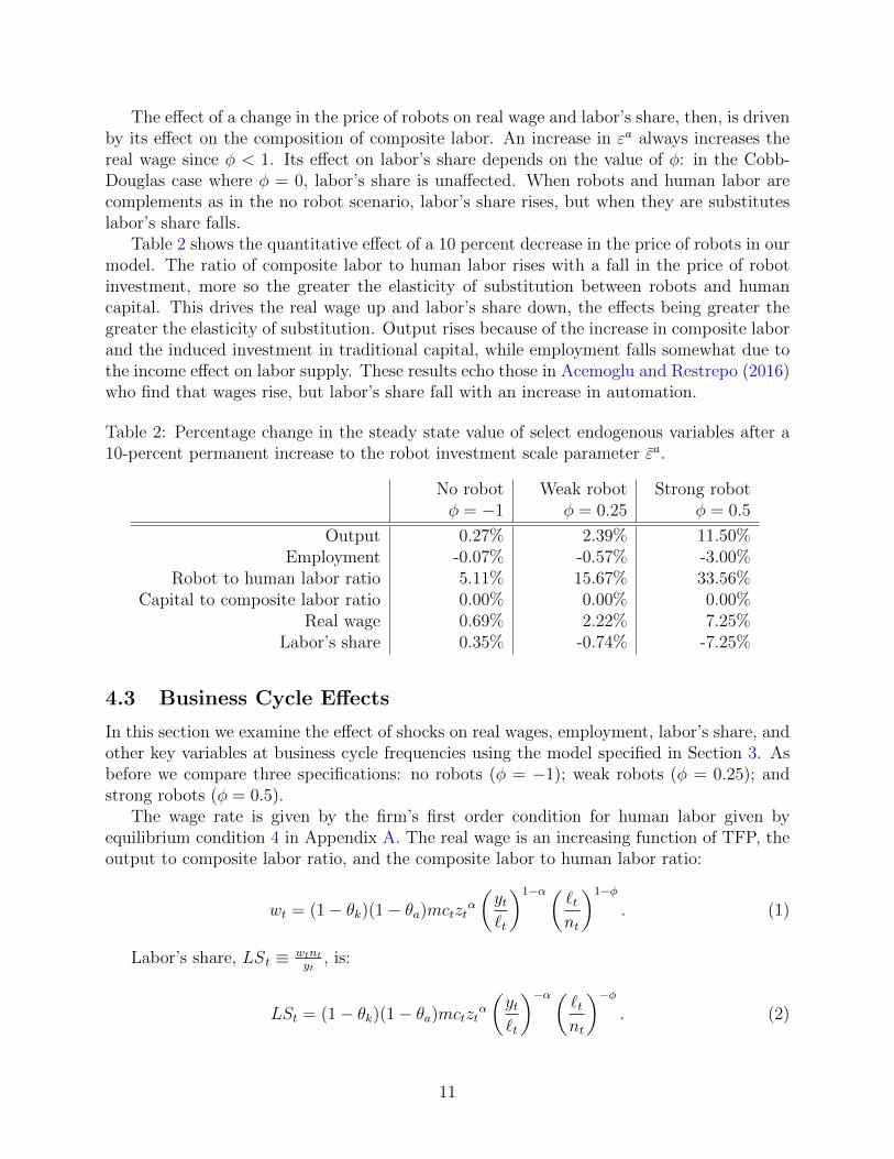
Table 2 shows the quantitative effect of a 10 percent decrease in the price of robots in ourmodel. The ratio of composite labor to human labor rises with a fall in the price of robotinvestment, more so the greater the elasticity of substitution between robots and humancapital. This drives the real wage up and labor’s share down, the effects being greater thegreater the elasticity of substitution. Output rises because of the increase in composite laborand the induced investment in traditional capital, while employment falls somewhat due tothe income effect on labor supply. These results echo those in Acemoglu and Restrepo (2016)who find that wages rise, but labor’s share fall with an increase in automation.
Table 2: Percentage change in the steady state value of select endogenous variables after a10-percent permanent increase to the robot investment scale parameter εa.
No robot Weak robot Strong robotφ = −1 φ = 0.25 φ = 0.5
Output 0.27% 2.39% 11.50%Employment -0.07% -0.57% -3.00%
Robot to human labor ratio 5.11% 15.67% 33.56%Capital to composite labor ratio 0.00% 0.00% 0.00%
Real wage 0.69% 2.22% 7.25%Labor’s share 0.35% -0.74% -7.25%
4.3 Business Cycle Effects
In this section we examine the effect of shocks on real wages, employment, labor’s share, andother key variables at business cycle frequencies using the model specified in Section 3. Asbefore we compare three specifications: no robots (φ = −1); weak robots (φ = 0.25); andstrong robots (φ = 0.5).
The wage rate is given by the firm’s first order condition for human labor given byequilibrium condition 4 in Appendix A. The real wage is an increasing function of TFP, theoutput to composite labor ratio, and the composite labor to human labor ratio:
wt = (1− θk)(1− θa)mctztα(yt`t
)1−α(`tnt
)1−φ
. (1)
Labor’s share, LSt ≡ wtntyt
, is:
LSt = (1− θk)(1− θa)mctztα(yt`t
)−α(`tnt
)−φ. (2)
11
Labor’s share is an increasing function of the output to composite labor ratio when α < 0and a decreasing function of the composite labor to human labor ratio when φ > 0.11 Notethat the output to composite labor ratio yt
`tincreases with the capital to composite labor
ratio kt`t
, and that the composite labor to human labor ratio `tnt
is an increasing functionof the robot to human labor ratio at
nt. In our analysis we will focus on the role these two
ratios—capital to composite labor kt`t
and robot to human labor atnt
—have on the real wageand labor’s share of income.
In equations (1) and (2), an increase in marginal cost or TFP increases real wages andlabor’s share. An increase in the capital to composite labor ratio and/or robot to humanlabor ratio increases the real wage. When α < 0 and φ > 0, as in the two specifications ofinterest in this paper, an increase in the capital to composite labor ratio increases labor’sshare while an increase in the robot to human labor ratio reduces labor’s share. Intuitively,increases in either the captial to composite labor ratio or the robot to human labor ratioraises the marginal product of human labor which in turn increases the real wage. Further,given that capital and human labor are complements, human labor rises with an increase inthe capital to composite labor ratio, leading to an increase in labor income. On the otherhand, while the real wage rises when the robot to human labor ratio increases, human laborfalls when the robot to human labor ratio rises leading to a smaller labor share of income.
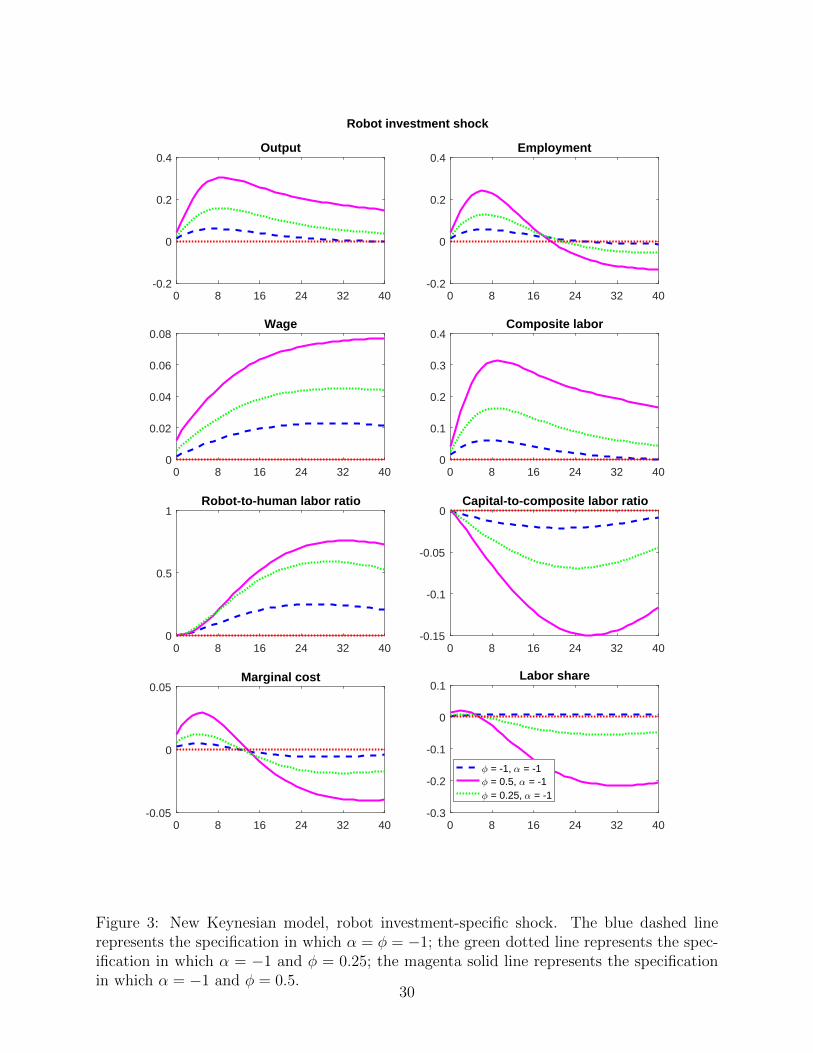
Figures 2 to 5 show the response of key variables to one percentage point increases in thefour disturbance terms—traditional capital, robot capital, TFP, and the nominal interestrate. The distinctive effects of robot capital are most apparent when we compare a shock tothe price of traditional capital shown in Figure 2 with a shock to the price of robot capitalshown in Figure 3. In each of these cases movements in marginal cost are minimal andTFP is constant, so movements in wages and labor’s share are dominated by the capital tocomposite labor ratio and the robot to human labor ratio.
A reduction in the price of traditional capital causes the household to increase investmentin traditional capital and substitute away from robot capital. The increased investmentdemand increases employment, output, and the real wage. The robot to human labor ratiofalls and the capital to composite labor ratio rises, leading to an increase in labor’s share.The increase in labor’s share is greater the more substitutable are robots and human labor.By contrast, while a decrease in the price of robot capital also increases employment, wages,and output, it increases the robot to human labor ratio and reduces the capital to compositelabor ratio, causing labor’s share to fall. Again, the decline in labor’s share is considerablylarger in the high substitutability case.
Figure 4 shows the response to a TFP shock. As is common in models with nominalrigidities, a positive TFP shock reduces demand for all three factors of production in theshort run because aggregate demand does not rise as much as potential output. While thereduction in input demand would lower rental rates and wages, wage rigidity along with alower aggregate price level raises the real wage while the rental rates fall. This makes humanlabor relatively more expensive which induces firms to substitute away from human labor infavor of both types of capital. This raises both the capital to composite labor ratio and therobot to human labor ratio. Overall, the rise in robot to human labor ratio and drop in the
11In other words, when traditional capital and composite labor are complements and when robots andhuman labor are substitutes.
12
marginal cost of production outweigh the rise in capital to composite labor ratio, leadingto a fall in labor’s share of income. Note that the greater the elasticity of substitutionbetween robots and human capital, the larger is the reallocation from human labor to robotcapital and the greater is the decline in labor’s share. It is worth noting that while the naıvecalibration of our model makes it more persistent, we do observe the overshooting of labor’sshare highlighted by Choi and Rıos-Rull (2009) under the no-robot scenario. In contrast,the presence of the robot capital lowers the labor’s share, and the labor’s share stays belowits steady state value until it returns to its steady state.
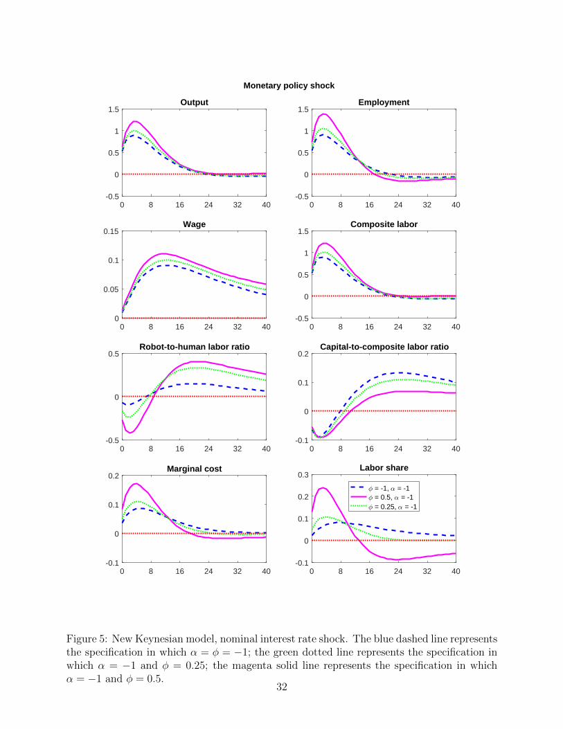
Finally, Figure 5 shows the response to a nominal interest rate shock. A reduction inthe nominal rate increases demand for output and therefore also for traditional capital,robots, and human labor. Factor prices rise in response to increased demand. In the periodimmediately following the shock, rental rates rise by more than real wages due to wagerigidity, leading firms to increase employment of human labor relative to traditional capitaland robots. Therefore both the capital to composite labor ratio and robot to human laborratio fall. Over time, however, accumulation of both types of capital reverses these effectsand the ratios rise. The net effect is for labor’s share to rise in the period immediatelyfollowing the decrease in interest rates. The increase in labor’s share is largest in the strongrobot case. In this case the reversal in labor’s share is also more dramatic, with the neteffect on labor’s share becoming negative after about 14 quarters.
4.4 Robots in a Frictionless Model
In this section we take a brief detour to examine the effect of shocks on wages, employment,labor’s share, and other key variables at business cycle frequencies using a real business cyclemodel modified to include robot capital alongside traditional capital. This model removesthe frictions from the New Keynesian model by setting the parameters h, κk, κa, νk, and νato zero, removing the monopolistic competitive intermediate good firms, and removing thelabor union. In addition there is no monetary policy component to this model. This modelhelps us isolate the effect of robots as the shocks operate through the production technologyand helps us understand the extent to which nominal rigidities interact with the presence ofrobot capital.
As in the previous section, the wage rate is given by the firm’s first order conditionfor human labor. This is identical to equilibrium condition 4 in Appendix A for the NewKeynesian model except that there is no marginal cost term in this model. The real wage isan increasing function of TFP, the output to composite labor ratio, and the composite laborto human labor ratio:
wt = (1− θk)(1− θa)ztα(yt`t
)1−α(`tnt
)1−φ
. (3)
Labor’s share, LSt ≡ wtntyt
, is:
LSt = (1− θk)(1− θa)ztα(yt`t
)−α(`tnt
)−φ. (4)
13
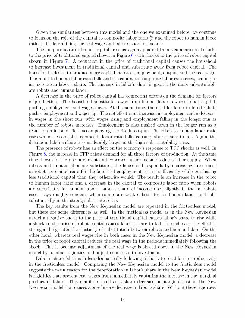
Given the similarities between this model and the one we examined before, we continueto focus on the role of the capital to composite labor ratio kt
`tand the robot to human labor
ratio atnt
in determining the real wage and labor’s share of income.The unique qualities of robot capital are once again apparent from a comparison of shocks
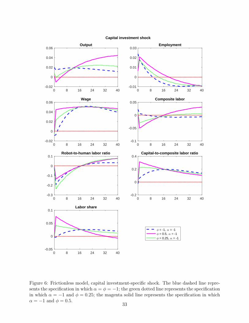
to the price of traditional capital shown in Figure 6 with shocks to the price of robot capitalshown in Figure 7. A reduction in the price of traditional capital causes the householdto increase investment in traditional capital and substitute away from robot capital. Thehousehold’s desire to produce more capital increases employment, output, and the real wage.The robot to human labor ratio falls and the capital to composite labor ratio rises, leading toan increase in labor’s share. The increase in labor’s share is greater the more substitutableare robots and human labor.
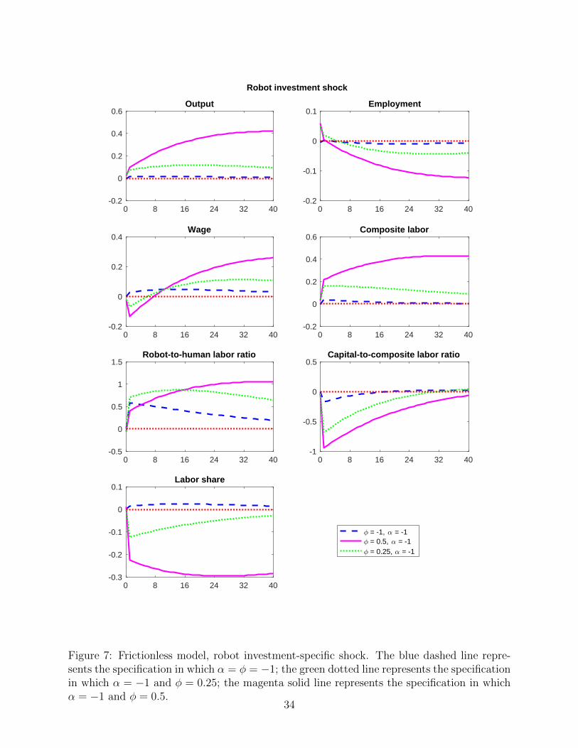
A decrease in the price of robot capital has competing effects on the demand for factorsof production. The household substitutes away from human labor towards robot capital,pushing employment and wages down. At the same time, the need for labor to build robotspushes employment and wages up. The net effect is an increase in employment and a decreasein wages in the short run, with wages rising and employment falling in the longer run asthe number of robots increases. Employment is also pushed down in the longer run as aresult of an income effect accompanying the rise in output. The robot to human labor ratiorises while the capital to composite labor ratio falls, causing labor’s share to fall. Again, thedecline in labor’s share is considerably larger in the high substitutability case.
The presence of robots has an effect on the economy’s response to TFP shocks as well. InFigure 8, the increase in TFP raises demand for all three factors of production. At the sametime, however, the rise in current and expected future income reduces labor supply. Whenrobots and human labor are substitutes the household responds by increasing investmentin robots to compensate for the failure of employment to rise sufficiently while purchasingless traditional capital than they otherwise would. The result is an increase in the robotto human labor ratio and a decrease in the capital to composite labor ratio when robotsare substitutes for human labor. Labor’s share of income rises slightly in the no robotscase, stays roughly constant when robots are weak substitutes for human labor, and fallssubstantially in the strong substitutes case.
The key results from the New Keynesian model are repeated in the frictionless model,but there are some differences as well. In the frictionless model as in the New Keynesianmodel a negative shock to the price of traditional capital causes labor’s share to rise whilea shock to the price of robot capital causes labor’s share to fall. In each case the effect isstronger the greater the elasticity of substitution between robots and human labor. On theother hand, whereas real wages rise in both cases in the New Keynesian model, a decreasein the price of robot capital reduces the real wage in the periods immediately following theshock. This is because adjustment of the real wage is slowed down in the New Keynesianmodel by nominal rigidities and adjustment costs to investment.
Labor’s share falls much less dramatically following a shock to total factor productivityin the frictionless model. Comparing the New Keynesian model to the frictionless modelsuggests the main reason for the deterioration in labor’s share in the New Keynesian modelis rigidities that prevent real wages from immediately capturing the increase in the marginalproduct of labor. This manifests itself as a sharp decrease in marginal cost in the NewKeynesian model that causes a one-for-one decrease in labor’s share. Without these rigidities,
14

labor’s share declines markedly only in the strong robot case.We conclude from this exercise that much of the response of labor’s share to shocks in
the New Keynesian model can be explained by the introduction of robots per se rather thanthe various rigidities included in the model. In the case of shocks to TFP, however, rigiditiesgreatly magnify the response of labor’s share.
4.5 Volatility and Correlations
The classic real business cycle model with a Cobb-Douglas production function yields alabor’s share that is constant over the business cycle. In the data, however, the contempora-neous correlation between output and labor’s share is negative, with estimates ranging from−0.11 by Choi and Rıos-Rull (2009) to −0.71 by Ambler and Cardia (1998). A number ofauthors have explored deviations from the textbook real business cycle model that can repli-cate this feature of the data, including Ambler and Cardia (1998) (imperfect competition inproduct markets); Gomme and Greenwood (1995) (optimal contracting between workers andentrepreneurs); Hansen and Prescott (2005) and Choi and Rıos-Rull (2009) (non-Walrasianlabor markets). Our purpose here is not to attempt the match the observed correlation inthe data, but to examine the effect of robots on these correlations.
We compute the analytical correlations between output, hours, and labor’s share in eachof the three specifications of our model from the transition equations implied by the solutionto the model. The results are summarized in Table 3. The first column shows the correlationbetween labor’s share and output and output and employment when the model is driven onlyby TFP shocks. Within each cell we show the correlation for the no robots, weak robots, andstrong robots specifications. The second through fourth columns show the same correlationswhen the model is driven only by shocks to the capital investment, robot investment, and thenominal interest rate respectively. In the last column all of the shocks are operative, with therelative variances of the shocks given by the estimation procedure described in Appendix B.The data correlation coefficients come from the quarterly U.S. real GDP, non-farm businesslabor’s share, and the non-farm business hours, de-trended using an Hodrick-Prescott filterwith a standard smoothing parameter of 1,600.12
12While we include the correlations in the data, the purpose of this paper is not to match empiricalmoments, but to explore the effects of robots in a business cycle model.
15
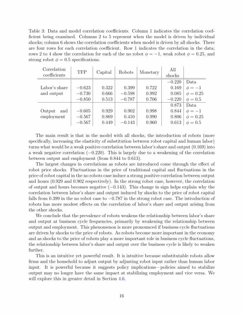
Table 3: Data and model correlation coefficients. Column 1 indicates the correlation coef-ficient being examined. Columns 2 to 5 represent when the model is driven by individualshocks; column 6 shows the correlation coefficients when model is driven by all shocks. Thereare four rows for each correlation coefficient. Row 1 indicates the correlation in the data;rows 2 to 4 show the correlation for each of the no robot φ = −1, weak robot φ = 0.25, andstrong robot φ = 0.5 specifications.
Correlationcoefficients
TFP Capital Robots MonetaryAll
shocks
Labor’s shareand output
−0.220 Data−0.623 0.322 0.399 0.722 0.169 φ = −1−0.730 0.666 −0.598 0.992 0.085 φ = 0.25−0.850 0.513 −0.787 0.706 −0.220 φ = 0.5
Output andemployment
0.873 Data−0.605 0.929 0.902 0.998 0.844 φ = −1−0.567 0.869 0.410 0.990 0.806 φ = 0.25−0.567 0.449 −0.143 0.960 0.613 φ = 0.5
The main result is that in the model with all shocks, the introduction of robots (morespecifically, increasing the elasticity of substitution between robot capital and human labor)turns what would be a weak positive correlation between labor’s share and output (0.169) intoa weak negative correlation (−0.220). This is largely due to a weakening of the correlationbetween output and employment (from 0.844 to 0.613).
The largest changes in correlations as robots are introduced come through the effect ofrobot price shocks. Fluctuations in the price of traditional capital and fluctuations in theprice of robot capital in the no robots case induce a strong positive correlation between outputand hours (0.929 and 0.902 respectively). In the strong robot case, however, the correlationof output and hours becomes negative (−0.143). This change in sign helps explain why thecorrelation between labor’s share and output induced by shocks to the price of robot capitalfalls from 0.399 in the no robot case to −0.787 in the strong robot case. The introduction ofrobots has more modest effects on the correlation of labor’s share and output arising fromthe other shocks.
We conclude that the prevalence of robots weakens the relationship between labor’s shareand output at business cycle frequencies, primarily by weakening the relationship betweenoutput and employment. This phenomenon is more pronounced if business cycle fluctuationsare driven by shocks to the price of robots. As robots become more important in the economyand as shocks to the price of robots play a more important role in business cycle fluctuations,the relationship between labor’s share and output over the business cycle is likely to weakenfurther.
This is an intuitive yet powerful result. It is intuitive because substitutable robots allowfirms and the household to adjust output by adjusting robot input rather than human laborinput. It is powerful because it suggests policy implications—policies aimed to stabilizeoutput may no longer have the same impact at stabilizing employment and vice versa. Wewill explore this in greater detail in Section 4.6.
16
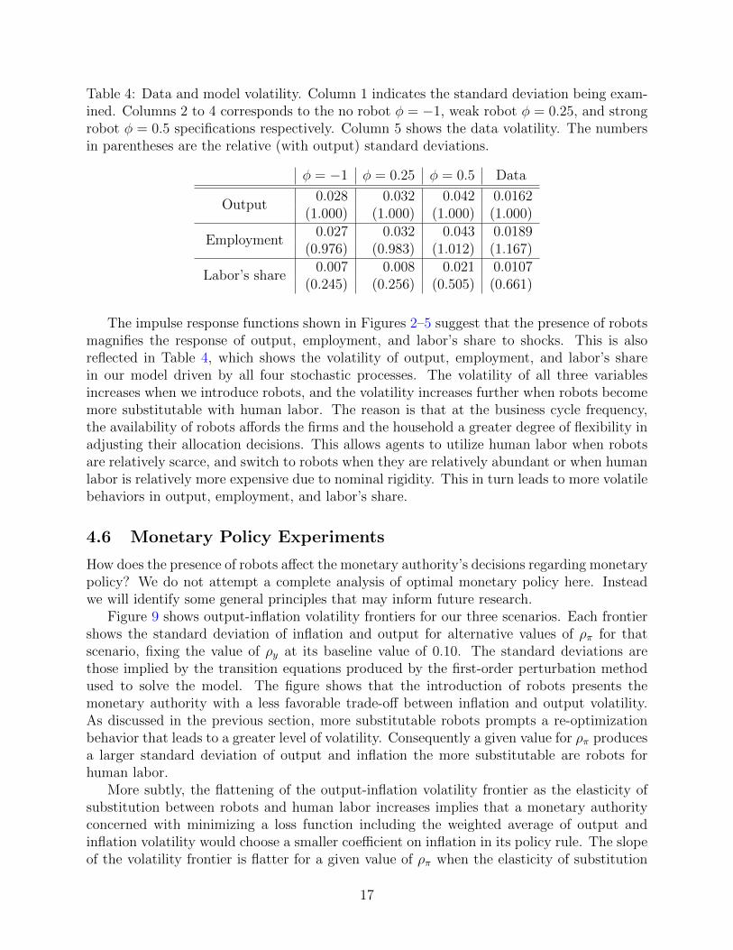
Table 4: Data and model volatility. Column 1 indicates the standard deviation being exam-ined. Columns 2 to 4 corresponds to the no robot φ = −1, weak robot φ = 0.25, and strongrobot φ = 0.5 specifications respectively. Column 5 shows the data volatility. The numbersin parentheses are the relative (with output) standard deviations.
φ = −1 φ = 0.25 φ = 0.5 Data
Output0.028 0.032 0.042 0.0162
(1.000) (1.000) (1.000) (1.000)
Employment0.027 0.032 0.043 0.0189
(0.976) (0.983) (1.012) (1.167)
Labor’s share0.007 0.008 0.021 0.0107
(0.245) (0.256) (0.505) (0.661)
The impulse response functions shown in Figures 2–5 suggest that the presence of robotsmagnifies the response of output, employment, and labor’s share to shocks. This is alsoreflected in Table 4, which shows the volatility of output, employment, and labor’s sharein our model driven by all four stochastic processes. The volatility of all three variablesincreases when we introduce robots, and the volatility increases further when robots becomemore substitutable with human labor. The reason is that at the business cycle frequency,the availability of robots affords the firms and the household a greater degree of flexibility inadjusting their allocation decisions. This allows agents to utilize human labor when robotsare relatively scarce, and switch to robots when they are relatively abundant or when humanlabor is relatively more expensive due to nominal rigidity. This in turn leads to more volatilebehaviors in output, employment, and labor’s share.
4.6 Monetary Policy Experiments
How does the presence of robots affect the monetary authority’s decisions regarding monetarypolicy? We do not attempt a complete analysis of optimal monetary policy here. Insteadwe will identify some general principles that may inform future research.
Figure 9 shows output-inflation volatility frontiers for our three scenarios. Each frontiershows the standard deviation of inflation and output for alternative values of ρπ for thatscenario, fixing the value of ρy at its baseline value of 0.10. The standard deviations arethose implied by the transition equations produced by the first-order perturbation methodused to solve the model. The figure shows that the introduction of robots presents themonetary authority with a less favorable trade-off between inflation and output volatility.As discussed in the previous section, more substitutable robots prompts a re-optimizationbehavior that leads to a greater level of volatility. Consequently a given value for ρπ producesa larger standard deviation of output and inflation the more substitutable are robots forhuman labor.
More subtly, the flattening of the output-inflation volatility frontier as the elasticity ofsubstitution between robots and human labor increases implies that a monetary authorityconcerned with minimizing a loss function including the weighted average of output andinflation volatility would choose a smaller coefficient on inflation in its policy rule. The slopeof the volatility frontier is flatter for a given value of ρπ when the elasticity of substitution
17
between robots and human labor is larger. This means that a further decrease in inflationvariability comes at a larger marginal cost in terms of output variability. Suppose the choiceof ρπ reflects the optimizing choice of a monetary authority that minimizes a loss functionwith a given weighting of inflation and output variability. This monetary authority wouldrespond to the increased marginal cost of inflation reduction introduced by the presenceof robots by choosing a smaller value of ρπ, moving up and to the left along the volatilityfrontier.
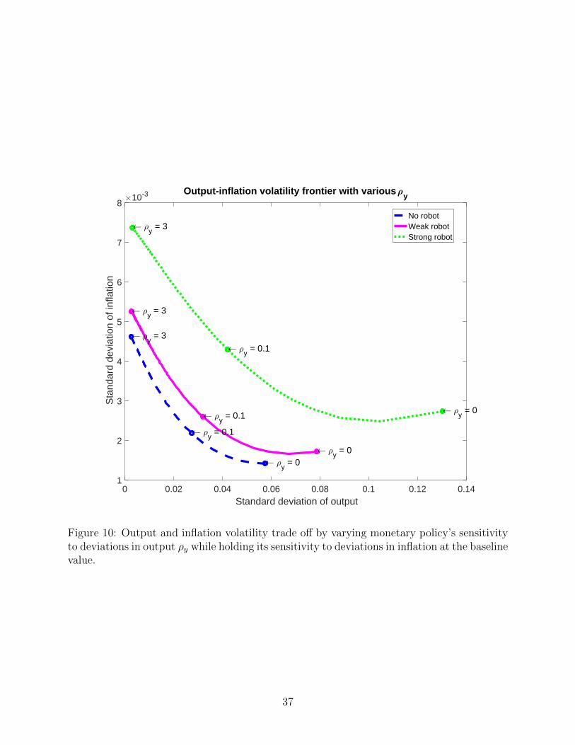
Figure 10 shows output-inflation volatility frontiers for different values of ρy holding ρπat its baseline value of 1.49. The figure shows the same deterioration in the output-inflationvariability trade-off as in Figure 9. While it is not apparent in the figure, there is a slightflattening in these volatility frontiers as in Figure 9, implying that an optimizing monetaryauthority would choose a point on the frontier further up and to the left—implying a largervalue of ρy—in the strong robot case. In sum, monetary authorities whose objective is tominimize a weighted average of output and inflation volatility would adopt a policy rule witha smaller emphasis on stabilizing inflation and a larger emphasis on stabilizing output in aworld where the elasticity of substitution between robots and human labor is larger.
A final implication for monetary policy involves the relationship between the volatilityof employment and output. Existing business cycle models do not typically distinguishbetween a monetary authority’s interest in stabilizing output and stabilizing employment.These objectives are assumed to be tightly connected by a “divine coincidence” similar tothat identified by Blanchard and Galı (2007) in reference to the inflation and output gapstabilization objectives. In the previous section, however, it is shown that the presence ofrobots reduces the correlation between output and employment. This has implications formonetary policy.
Figure 11 shows the standard deviation of output and employment implied by the sce-narios of our model when the coefficient on inflation in the monetary policy rule is set at itsbaseline value and the coefficient on output is varied. In all scenarios a larger coefficient onoutput reduces the standard deviation of employment along with that of output. However,in the two robot scenarios the standard deviation of employment is larger for any given stan-dard deviation of output. Furthermore, if we imagine drawing a horizontal line at a givenvalue of σn we see that the monetary authority would have to adopt a higher value of ρyto achieve a given amount of employment stabilization in a world with highly substitutablerobots. Thus to the extent that monetary authorities value employment stabilization apartfrom output stabilization, the presence of robots requires a greater commitment to outputstabilization.
5 Conclusion
In this paper we explore how the inclusion of human labor-replacing capital, or robots,affects the relationship between output, employment, and labor’s share of income in a NewKeynesian model. We find that a permanent reduction in the price of robots causes outputto rise, wages to rise, and labor’s share to fall.
At the business cycle frequency, a shock lowering the price of traditional capital causeslabor’s share to rise while a shock lowering the price of robot capital causes labor’s share to
18
fall. A positive shock to total factor productivity causes labor’s share to fall, largely due tointeractions between robots and nominal rigidities. All of these effects are greater the higheris the elasticity of substitution between robots and human labor. An expansionary monetarypolicy shock increases labor’s share in the short run, but when robots and human labor aresufficiently substitutable, the labor’s share dips below its steady state before returning to itssteady state.
The presence of robots weakens the correlation between output and labor’s share, pri-marily by weakening the correlation between output and employment. This effect is largerwhen robots become more substitutable with human labor and when shocks to the price ofrobot investment goods take on a greater role in the economy. The presence of robots alsoincreases volatility of output, inflation, and employment.
Finally, the presence of robots has implications for monetary policy. In a world whererobot capital plays a more prominent role, our model suggests that monetary policymakersseeking to stabilize output and inflation would need to adopt a monetary policy rule thatplaces less emphasis on inflation and more emphasis on output. A monetary policymakerwith a separate interest in stabilizing employment would need to emphasize the stabilizationof output to an even greater extent.
References
Acemoglu, D. and D. Autor (2011): “Skills, Tasks and Technologies: Implicationsfor Employment and Earnings,” in Handbook of Labor Economics, ed. by D. Card andO. Ashenfelter, Elsevier, vol. 4, Part B of Handbook of Labor Economics, chap. 12, 1043–1171.
Acemoglu, D. and P. Restrepo (2016): “The Race Between Machine and Man: Im-plications of Technology for Growth, Factor Shares and Employment,” Working Paper22252, National Bureau of Economic Research.
Ambler, S. and E. Cardia (1998): “The Cyclical Behaviour of Wages and Profits underImperfect Competition,” The Canadian Journal of Economics, 31, 148–164.
Autor, D. H. (2015): “Why Are There Still So Many Jobs? The History and Future ofWorkplace Automation,” Journal of Economic Perspectives, 29, 3–30.
Bessen, J. (2015): “Toil and Technology,” Finance & Development, 52.
Blanchard, O. and J. Galı (2007): “Real Wage Rigidities and the New KeynesianModel,” Journal of Money, Credit and Banking, 39, 35–65.
Boldrin, M. and M. Horvath (1995): “Labor Contracts and Business Cycles,” Journalof Political Economy, 103, 972–1004.
Brynjolfsson, E. and A. McAfee (2014): The Second Machine Age: Work, Progress,and Prosperity in a Time of Brilliant Technologies, W. W. Norton.
19
Byrne, D. and C. Corrado (2017): “ICT Prices and ICT Services: What do they tellus about Productivity and Technology?” Finance and Economics Discussion Series.
Calvo, G. A. (1983): “Staggered prices in a utility-maximizing framework,” Journal ofMonetary Economics, 12, 383–398.
Chirinko, R. S. (2008): “σ: The Long And Short Of It,” CESifo Working Paper Series2234, CESifo Group Munich.
Choi, S. and J.-V. Rıos-Rull (2009): “Understanding the Dynamics of Labor Share:the Role of Noncompetitive Factor Prices,” Annals of Economics and Statistics, 251–277.
Gomme, P. and J. Greenwood (1995): “On the cyclical allocation of risk,” Journal ofEconomic Dynamics and Control, 19, 91 – 124.
Hansen, G. D. and E. C. Prescott (2005): “Capacity constraints, asymmetries, andthe business cycle,” Review of Economic Dynamics, 8, 850 – 865.
Justiniano, A., G. E. Primiceri, and A. Tambalotti (2010): “Investment shocksand business cycles,” Journal of Monetary Economics, 57, 132–145.
Krugman, P. (2012): “Rise of the Robots,” http://krugman.blogs.nytimes.com/2012/
12/08/rise-of-the-robots/.
Krusell, P., L. E. Ohanian, J.-V. Rıos-Rull, and G. L. Violante (2000): “Capital-skill Complementarity and Inequality: A Macroeconomic Analysis,” Econometrica, 68,1029–1053.
Leontief, W. (1983): “National Perspective: The Definition of Problems and Oppor-tunities,” in The Long-Term Impact of Technology on Employment and Unemployment,National Academy of Engineering, 3–7.
Pratt, G. A. (2015): “Is a Cambrian Explosion Coming for Robotics?” Journal of Eco-nomic Perspectives, 29, 51–60.
Shermis, M. D. and B. Hamner (2013): “Contrasting State-of-the-Art Automated Scor-ing of Essays: Analysis,” in Handbook of Automated Essay Evaluation: Current Applica-tions and New Directions, ed. by M. D. Shermis and J. Burstein, Routledge, Handbook ofAutomated Essay Evaluation: Current Applications and New Directions, chap. 19.
Smets, F. and R. Wouters (2005): “Comparing Shocks and Frictions in US and EuroArea Business Cycles: A Bayesian DSGE Approach,” Journal of Applied Econometrics,20, 161–183.
Summers, L. H. (2013): “Economic Possibilities for Our Children,” National Bureau ofEconomic Research, no. 4 in NBER Reporters OnLine, the 2013 Martin Feldstein Lecture.
20
A Equilibrium Conditions
A.1 Equilibrium Conditions
A.1.1 Production
1. Composite labor:
`t =[θa (µat at)
φ + (1− θa)ntφ] 1φ
2. Capital demand:
rkt = mctθkztα
(ytµkt kt
)1−α
3. Robot demand:
rat = mct(1− θk)ztα(yt`t
)1−α
θa
(`tµat at
)1−φ
4. Human labor demand:
wt = mct(1− θk)ztα(yt`t
)1−α
(1− θa)(`tnt
)1−φ
5. Price optimality:xy1,t = εyx
y2,t
6. Auxiliary variable:
xy1,t = pt
[Λtyt + βλyEt
1
pt+1
(πtηy
πt+1
) 11−εy
xy1,t+1
]
7. Auxiliary variable:
xy2,t = Λtytmct + βλyEt(πtηy
πt+1
) εy1−εy
xy2,t+1
8. Relative price:
p1
1−εyt =
1− λy(πt−1
ηy
πt
) 11−εy
1− λy
A.1.2 Household
9. Capital law of motion:
kt+1 = (1− δk)kt + εkt
[1− Sk
(iktikt−1
)]ikt
21

10. Robot law of motion:
at+1 = (1− δa)at + εat
[1− Sa
(iatiat−1
)]iat
11. Consumption:Λt = εbt (ct − hct−1)−γ − hβEtεbt+1 (ct+1 − hct)−γ
12. Physical capital:
Λtqkt = βEtΛt+1
[rkt+1µ
kt+1 −Ψk
(µkt+1
)+ qkt+1(1− δk)
]13. Robots:
Λtqat = βEtΛt+1
[rat+1µ
at+1 −Ψa
(µat+1
)+ qat+1(1− δa)
]14. Physical capital investment:
Λt = Λtqkt εkt
[1− Sk
(iktikt−1
)− Sk ′
(iktikt−1
)iktikt−1
]+ βEtΛt+1q
kt+1ε
kt+1Sk
′(ikt+1
ikt
)(ikt+1
ikt
)2
15. Robot investment:
Λt = Λtqat εat
[1− Sa
(iatiat−1
)− Sa′
(iatiat−1
)iatiat−1
]+ βEtΛt+1q
at+1ε
at+1Sa
′(iat+1
iat
)(iat+1
iat
)2
16. Physical capital utilization:rkt = Ψk ′ (µkt )
17. Robot utilization:rat = Ψa′ (µat )
18. Bonds:
Λt = βEtΛt+1Rt
πt+1
A.1.3 Wage Setting
19. Wage optimality:xw1,t = εnκnx
2w,t
20. Auxiliary variable:
xw1,t = w1−εn(1+σ)
1−εnt
[Λtntwt
−εn1−εn + βλnEtw
−1+εn(1+σ)1−εn
t+1
(πtηw
πt+1
) 11−εn
xw1,t+1
]21. Auxiliary variable:
xw2,t = εbtnt1+σwt
−εn(1+σ)1−εn + βλnEt
(πtηw
πt+1
) εn(1+σ)1−εn
xw2,t+1
22. Wage index:
wt1
1−εn = (1− λn)w1
1−εnt + λn
(wt−1
πt−1ηw
πt
) 11−εn
22
A.1.4 Stochastic Processes
23. Productivity process:
ln zt = (1− ρz) lnµz + ρz ln zt−1 + ςzηzt
24. Robot investment disturbances:
ln εat = (1− ρa) lnµεa + ρa ln εat−1 + ςaηat
25. Capital investment disturbances:
ln εkt = (1− ρk) lnµεk + ρk ln εkt−1 + ςkηkt
26. Demand disturbances:
ln εbt = (1− ρb) lnµεb + ρb ln εbt−1 + ςbηbt
27. Taylor rule disturbances:
ln εmpt = (1− ρmp) lnµεmp + ρmp ln εmpt−1 + ςmpηmpt
A.1.5 Monetary Authority
29. Taylor rule: (Rt
R∗
)=
(Rt−1
R∗
)ρR [( πtπ∗
)ρπ ( yty∗
)ρY ]1−ρRεmpt
A.1.6 Resource Constraint
30. Resource constraint:
yt = ct + ikt + iat + Ψk(µkt)kt + Ψa (µat ) at
31. Aggregate demand:yt = p∗ty
∗t
32. Aggregate labor demand:nt = w∗tn
∗t
33. Aggregate supply:
y∗t = zt
[θk
(kt`t
)α
+ (1− θk)
] 1α[θa
(atnt
)φ+ (1− θa)
] 1φ
nt
34. Price distortion:
p∗t−1 = (1− λy)pt
εy1−εy + λyp
∗t−1−1(πt−1
ηy
πt
) εy1−εy
35. Wage distortion:
w∗t−1 = (1− λn)
(wtwt
) εn1−εn
+ λnw∗t−1−1(wt−1wt
πt−1ηw
πt
) εn1−εn
23
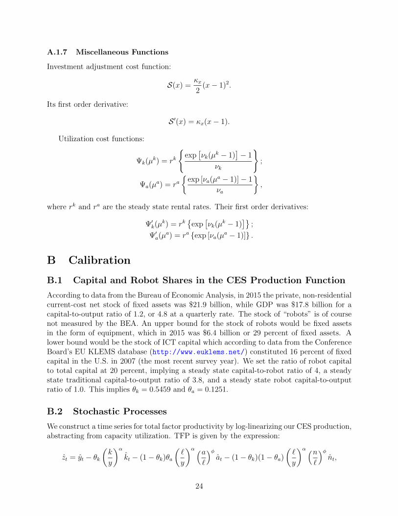
A.1.7 Miscellaneous Functions
Investment adjustment cost function:
S(x) =κx2
(x− 1)2.
Its first order derivative:
S ′(x) = κx(x− 1).
Utilization cost functions:
Ψk(µk) = rk
{exp
[νk(µ
k − 1)]− 1
νk
};
Ψa(µa) = ra
{exp [νa(µ
a − 1)]− 1
νa
},
where rk and ra are the steady state rental rates. Their first order derivatives:
Ψ′k(µk) = rk
{exp
[νk(µ
k − 1)]}
;
Ψ′a(µa) = ra {exp [νa(µ
a − 1)]} .
B Calibration
B.1 Capital and Robot Shares in the CES Production Function
According to data from the Bureau of Economic Analysis, in 2015 the private, non-residentialcurrent-cost net stock of fixed assets was $21.9 billion, while GDP was $17.8 billion for acapital-to-output ratio of 1.2, or 4.8 at a quarterly rate. The stock of “robots” is of coursenot measured by the BEA. An upper bound for the stock of robots would be fixed assetsin the form of equipment, which in 2015 was $6.4 billion or 29 percent of fixed assets. Alower bound would be the stock of ICT capital which according to data from the ConferenceBoard’s EU KLEMS database (http://www.euklems.net/) constituted 16 percent of fixedcapital in the U.S. in 2007 (the most recent survey year). We set the ratio of robot capitalto total capital at 20 percent, implying a steady state capital-to-robot ratio of 4, a steadystate traditional capital-to-output ratio of 3.8, and a steady state robot capital-to-outputratio of 1.0. This implies θk = 0.5459 and θa = 0.1251.
B.2 Stochastic Processes
We construct a time series for total factor productivity by log-linearizing our CES production,abstracting from capacity utilization. TFP is given by the expression:
zt = yt − θk(k
y
)αkt − (1− θk)θa
(`
y
)α (a`
)φat − (1− θk)(1− θa)
(`
y
)α (n`
)φnt,
24

where the “hat” variables indicate log-deviation from steady state. Parameter values arecalibrated according to Section 4.1, and the steady state ratios are computed using theparameters. Our data for output, traditional capital stock, robot capital stock, and hoursare from the Conference Board’s EU-KLEMS database (http://www.euklems.net/). Datafor capital inputs is from the November 2009 release of the USA-NAICS database. Datafor output and hours is from the March 2013 USA Basic Tables database. We use data forthe period 1977–2007. All data is annual. The data series with EU-KLEMS mnemonics inparentheses are:
• Gross output, volume indices, total industries, 2005 = 100 (GO QI);
• Hours worked, volume indices, 2005 = 100 (H EMP QI);
• Real fixed capital stock, 1995 prices, non-ICT assets, total industries (K NonICT);
• Real fixed capital stock, 1995 prices, ICT assets, total industries (K ICT).
Each series is logged and de-trended using the Hodrick-Prescott filter.The resulting annual series for zt is then converted to quarterly frequency using the cubic
spline method in Eviews. We estimate an AR(1) process for this series over the period1978:Q1-2007:Q4. The estimated persistence parameter is ρz = 0.9854 and the standarddeviation of the innovations is ςz = 0.0023.
We use the price of non-ICT capital and ICT capital from the EU-KLEMS database toproxy for the price of traditional and robot capital in our model. The precise series are:
• Gross fixed capital formation price index, 1995 = 1.0, total industries, non-ICT capital(Ip NonICT);
• Gross fixed capital formation price index, 1995 = 1.0, total industries, ICT capital(Ip ICT).
Each series is deflated by the PCE deflator from the Bureau of Economic Analysis. We thenlog and de-trend each series using the Hodrick-Prescott filter. As with TFP, we convertthe price series to the quarterly frequency using the cubic spline method and then estimateAR(1) process for each series. For the price of ICT capital the persistence parameter isρa = 0.9652 and the standard deviation of the innovations is ςz = 0.0079. For the price ofnon-ICT capital the persistence parameter is ρk = 0.9662 and the standard deviation of theinnovations is ςk = 0.0035.
To estimate the monetary policy shock process we estimate a monetary policy rule forthe U.S. from 1990:Q1-2007:Q4:
Rt = R∗ + β1Rt−1 + β2πt + β3yt + ηRt .
The data is quarterly from the St. Louis Federal Reserve Economic Database (FRED).The interest rate Rt is the effective federal funds rate (FEDFUNDS). The inflation rate πt isthe 4-quarter percentage change in the PCE price index (PCECTPI). The output gap yt isthe percentage difference between real GDP (GDPC1) and potential real GDP as measuredby the Congressional Budget Office (GDPPOT). We then estimate an AR(1) process for the
25

estimated monetary policy residual ηt. We arrive at a persistence parameter ρmp = 0.7063and a standard deviation for the innovates ςmp = 0.0007.
Lastly, our preference stochastic process is taken from estimates in Justiniano, Primiceri,and Tambalotti (2010).
26
1950 1955 1960 1965 1970 1975 1980 1985 1990 1995 2000 2005 2010 2015Shaded area indicate U.S. recessions
96
98
100
102
104
106
108
110
112
114
Labo
r sh
are
in n
on-f
arm
bus
ines
s se
ctor
, 200
9=10
0
Figure 1: Non-farm business sector labor’s share. Source: Bureau of Labor Statistics; seriesPRS85006173.
27
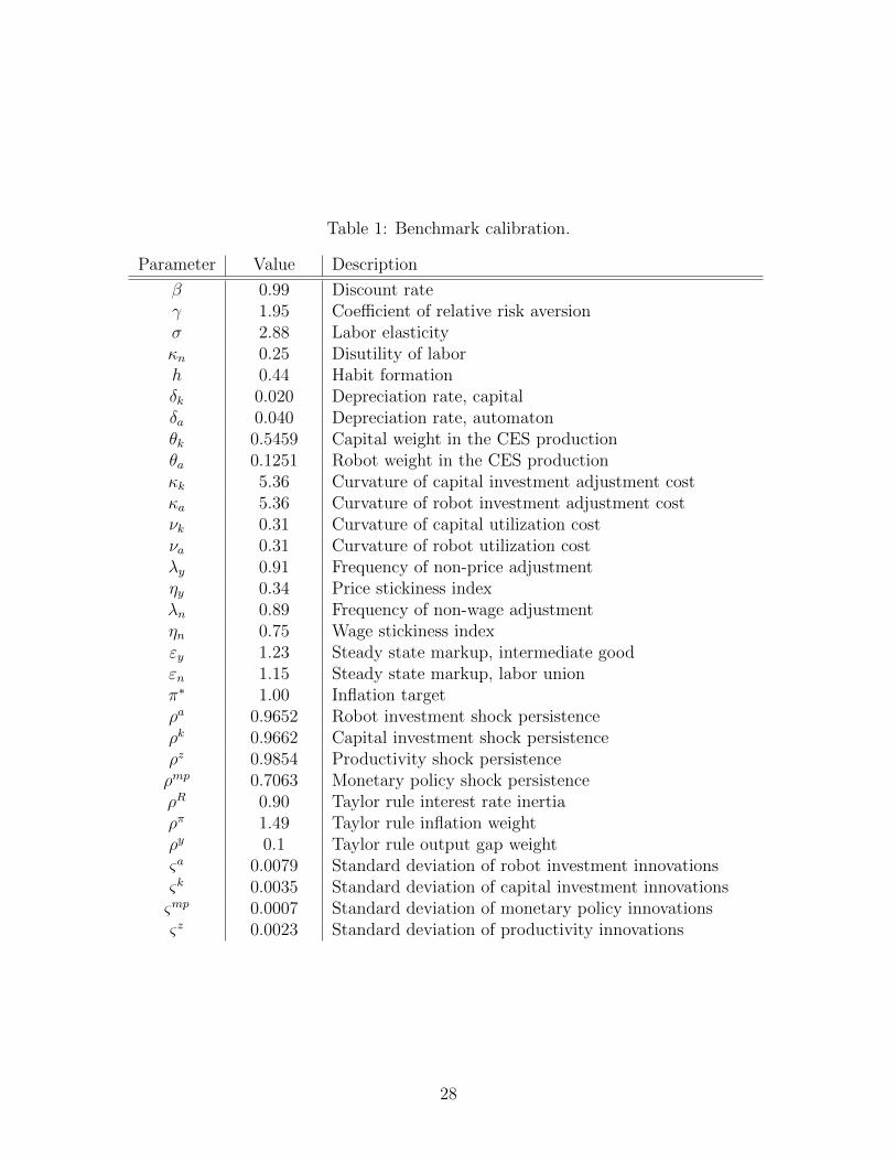
Table 1: Benchmark calibration.
Parameter Value Description
β 0.99 Discount rateγ 1.95 Coefficient of relative risk aversionσ 2.88 Labor elasticityκn 0.25 Disutility of laborh 0.44 Habit formationδk 0.020 Depreciation rate, capitalδa 0.040 Depreciation rate, automatonθk 0.5459 Capital weight in the CES productionθa 0.1251 Robot weight in the CES productionκk 5.36 Curvature of capital investment adjustment costκa 5.36 Curvature of robot investment adjustment costνk 0.31 Curvature of capital utilization costνa 0.31 Curvature of robot utilization costλy 0.91 Frequency of non-price adjustmentηy 0.34 Price stickiness indexλn 0.89 Frequency of non-wage adjustmentηn 0.75 Wage stickiness indexεy 1.23 Steady state markup, intermediate goodεn 1.15 Steady state markup, labor unionπ∗ 1.00 Inflation targetρa 0.9652 Robot investment shock persistenceρk 0.9662 Capital investment shock persistenceρz 0.9854 Productivity shock persistenceρmp 0.7063 Monetary policy shock persistenceρR 0.90 Taylor rule interest rate inertiaρπ 1.49 Taylor rule inflation weightρy 0.1 Taylor rule output gap weightςa 0.0079 Standard deviation of robot investment innovationsςk 0.0035 Standard deviation of capital investment innovationsςmp 0.0007 Standard deviation of monetary policy innovationsςz 0.0023 Standard deviation of productivity innovations
28

Capital investment shock
0 8 16 24 32 400
0.02
0.04
0.06Output
0 8 16 24 32 40-0.02
0
0.02
0.04
0.06Employment
0 8 16 24 32 400
0.01
0.02
0.03Wage
0 8 16 24 32 40-0.02
0
0.02
0.04
0.06Composite labor
0 8 16 24 32 40-0.06
-0.04
-0.02
0Robot-to-human labor ratio
0 8 16 24 32 40-0.05
0
0.05
0.1Capital-to-composite labor ratio
0 8 16 24 32 40-0.005
0
0.005
0.01Marginal cost
0 8 16 24 32 400
0.01
0.02
0.03Labor share
= -1, = -1 = 0.5, = -1 = 0.25, = -1
Figure 2: New Keynesian model, capital investment-specific shock. The blue dashed linerepresents the specification in which α = φ = −1; the green dotted line represents the spec-ification in which α = −1 and φ = 0.25; the magenta solid line represents the specificationin which α = −1 and φ = 0.5.
29
Robot investment shock
0 8 16 24 32 40-0.2
0
0.2
0.4Output
0 8 16 24 32 40-0.2
0
0.2
0.4Employment
0 8 16 24 32 400
0.02
0.04
0.06
0.08Wage
0 8 16 24 32 400
0.1
0.2
0.3
0.4Composite labor
0 8 16 24 32 400
0.5
1Robot-to-human labor ratio
0 8 16 24 32 40-0.15
-0.1
-0.05
0Capital-to-composite labor ratio
0 8 16 24 32 40-0.05
0
0.05Marginal cost
0 8 16 24 32 40-0.3
-0.2
-0.1
0
0.1Labor share
= -1, = -1 = 0.5, = -1 = 0.25, = -1
Figure 3: New Keynesian model, robot investment-specific shock. The blue dashed linerepresents the specification in which α = φ = −1; the green dotted line represents the spec-ification in which α = −1 and φ = 0.25; the magenta solid line represents the specificationin which α = −1 and φ = 0.5.
30

TFP shock
0 8 16 24 32 40-0.1
0
0.1
0.2
0.3Output
0 8 16 24 32 40-0.6
-0.4
-0.2
0
0.2Employment
0 8 16 24 32 400
0.05
0.1
0.15
0.2Wage
0 8 16 24 32 40-0.4
-0.2
0
0.2Composite labor
0 8 16 24 32 400
0.1
0.2
0.3
0.4Robot-to-human labor ratio
0 8 16 24 32 400
0.05
0.1Capital-to-composite labor ratio
0 8 16 24 32 40-0.3
-0.2
-0.1
0Marginal cost
0 8 16 24 32 40-0.3
-0.2
-0.1
0Labor share
= -1, = -1 = 0.5, = -1 = 0.25, = -1
Figure 4: New Keynesian model, TFP shock. The blue dashed line represents the specifica-tion in which α = φ = −1; the green dotted line represents the specification in which α = −1and φ = 0.25; and the magenta solid line represents the specification in which α = −1 andφ = 0.5.
31
Monetary policy shock
0 8 16 24 32 40-0.5
0
0.5
1
1.5Output
0 8 16 24 32 40-0.5
0
0.5
1
1.5Employment
0 8 16 24 32 400
0.05
0.1
0.15Wage
0 8 16 24 32 40-0.5
0
0.5
1
1.5Composite labor
0 8 16 24 32 40-0.5
0
0.5Robot-to-human labor ratio
0 8 16 24 32 40-0.1
0
0.1
0.2Capital-to-composite labor ratio
0 8 16 24 32 40-0.1
0
0.1
0.2Marginal cost
0 8 16 24 32 40-0.1
0
0.1
0.2
0.3Labor share
= -1, = -1 = 0.5, = -1 = 0.25, = -1
Figure 5: New Keynesian model, nominal interest rate shock. The blue dashed line representsthe specification in which α = φ = −1; the green dotted line represents the specification inwhich α = −1 and φ = 0.25; the magenta solid line represents the specification in whichα = −1 and φ = 0.5.
32
Capital investment shock
0 8 16 24 32 40-0.02
0
0.02
0.04
0.06Output
0 8 16 24 32 40-0.01
0
0.01
0.02
0.03Employment
0 8 16 24 32 40-0.02
0
0.02
0.04
0.06Wage
0 8 16 24 32 40-0.1
-0.05
0
0.05Composite labor
0 8 16 24 32 40-0.3
-0.2
-0.1
0
0.1Robot-to-human labor ratio
0 8 16 24 32 40-0.2
0
0.2
0.4Capital-to-composite labor ratio
0 8 16 24 32 40-0.05
0
0.05
0.1Labor share
= -1, = -1 = 0.5, = -1 = 0.25, = -1
Figure 6: Frictionless model, capital investment-specific shock. The blue dashed line repre-sents the specification in which α = φ = −1; the green dotted line represents the specificationin which α = −1 and φ = 0.25; the magenta solid line represents the specification in whichα = −1 and φ = 0.5.
33
Robot investment shock
0 8 16 24 32 40-0.2
0
0.2
0.4
0.6Output
0 8 16 24 32 40-0.2
-0.1
0
0.1Employment
0 8 16 24 32 40-0.2
0
0.2
0.4Wage
0 8 16 24 32 40-0.2
0
0.2
0.4
0.6Composite labor
0 8 16 24 32 40-0.5
0
0.5
1
1.5Robot-to-human labor ratio
0 8 16 24 32 40-1
-0.5
0
0.5Capital-to-composite labor ratio
0 8 16 24 32 40-0.3
-0.2
-0.1
0
0.1Labor share
= -1, = -1 = 0.5, = -1 = 0.25, = -1
Figure 7: Frictionless model, robot investment-specific shock. The blue dashed line repre-sents the specification in which α = φ = −1; the green dotted line represents the specificationin which α = −1 and φ = 0.25; the magenta solid line represents the specification in whichα = −1 and φ = 0.5.
34

TFP shock
0 8 16 24 32 400
0.1
0.2
0.3
0.4Output
0 8 16 24 32 40-0.06
-0.04
-0.02
0
0.02Employment
0 8 16 24 32 400
0.1
0.2
0.3Wage
0 8 16 24 32 40-0.1
0
0.1
0.2Composite labor
0 8 16 24 32 40-0.2
0
0.2
0.4
0.6Robot-to-human labor ratio
0 8 16 24 32 40-0.1
0
0.1
0.2Capital-to-composite labor ratio
0 8 16 24 32 40-0.15
-0.1
-0.05
0
0.05Labor share
= -1, = -1 = 0.5, = -1 = 0.25, = -1
Figure 8: Frictionless model, TFP shock. The blue dashed line represents the specificationin which α = φ = −1; the green dotted line represents the specification in which α = −1and φ = 0.25; and the magenta solid line represents the specification in which α = −1 andφ = 0.5.
35

0.025 0.03 0.035 0.04 0.045 0.05 0.055Standard deviation of output
0
1
2
3
4
5
6
7
Sta
ndar
d de
viat
ion
of in
flatio
n
10-3 Output-inflation volatility frontier with various
= 1.49
= 1.49
= 1.49
= 1
= 1
= 1
= 4 = 4
= 4
No robotWeak robotStrong robot
Figure 9: Output and inflation volatility trade off by varying monetary policy’s sensitivity todeviations in inflation ρπ while holding its sensitivity to deviations in output at the baselinevalue.
36
0 0.02 0.04 0.06 0.08 0.1 0.12 0.14Standard deviation of output
1
2
3
4
5
6
7
8
Sta
ndar
d de
viat
ion
of in
flatio
n
10-3 Output-inflation volatility frontier with various y
y = 0.1
y = 0.1
y = 0.1
y = 0
y = 0
y = 0
y = 3
y = 3
y = 3
No robotWeak robotStrong robot
Figure 10: Output and inflation volatility trade off by varying monetary policy’s sensitivityto deviations in output ρy while holding its sensitivity to deviations in inflation at the baselinevalue.
37
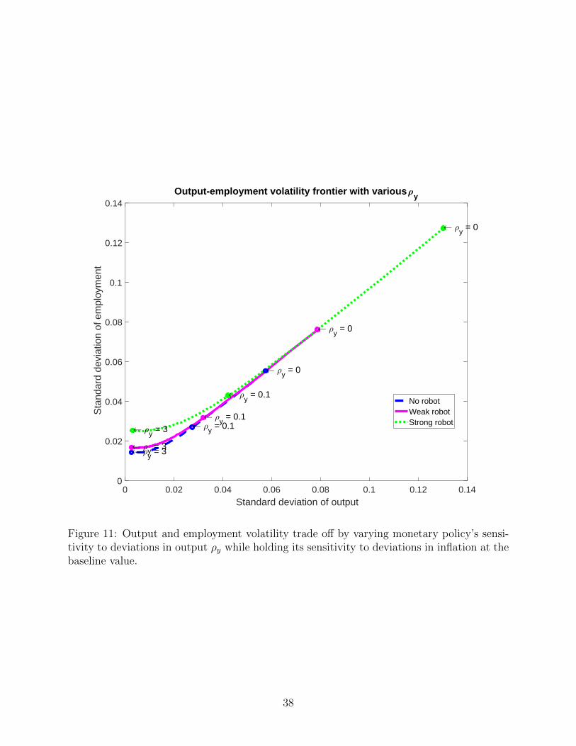
0 0.02 0.04 0.06 0.08 0.1 0.12 0.14Standard deviation of output
0
0.02
0.04
0.06
0.08
0.1
0.12
0.14
Sta
ndar
d de
viat
ion
of e
mpl
oym
ent
Output-employment volatility frontier with various y
y = 0.1
y = 0.1
y = 0.1
y = 0
y = 0
y = 0
y = 3
y = 3
y = 3
No robotWeak robotStrong robot
Figure 11: Output and employment volatility trade off by varying monetary policy’s sensi-tivity to deviations in output ρy while holding its sensitivity to deviations in inflation at thebaseline value.
38