1

A New Feature Parametrization for Monocular

SLAM using Line Features

Liang Zhao, Shoudong Huang, Lei Yan and Gamini Dissanayake

Abstract

This paper presents a new monocular SLAM algorithm that uses straight lines extracted from

images to represent the environment. A line is parametrized by two pairs of azimuth and elevation

angles together with the two corresponding camera centres as anchors making the feature initialization

relatively straightforward. There is no redundancy in the state vector as this is a minimal representation. A

bundle adjustment (BA) algorithm that minimizes the reprojection error of the line features is developed

for solving the monocular SLAM problem with only line features. A new map joining algorithm which

can automatically optimize the relative scales of the local maps is used to combine the local maps

generated using BA. Results from both simulations and experimental datasets are used to demonstrate

the accuracy and consistency of the proposed BA and map joining algorithms.

I. INTRODUCTION

Simultaneous localization and mapping (SLAM) is the problem where a mobile robot needs

to build a map of its environments and simultaneously use the map to locate itself. Monocular

L. Zhao, S. Huang and G. Dissanayake are with the Centre for Autonomous Systems, Faculty of Engineering and Infor-

mation Technology, University of Technology, Sydney, NSW 2007, Australia. {Liang.Zhao-1, Shoudong.Huang,

Gamini.Dissanayake} @uts.edu.au

L. Yan is with the Institute of Remote Sensing and GIS, School of Earth and Space Science, Peking University, Beijing,

China, 100871. lyan@pku.edu.cn

Corresponding author Liang.Zhao-1@uts.edu.au

2

SLAM is the SLAM problem where the only sensor onboard the robot for observing the

environment is a single camera [1], which is more challenging than the SLAM problems using

laser sensors and/or RGB-D cameras because of the lack of depth information from the sensor

measurements.

Point features are commonly used in monocular SLAM because they are relatively easy to

extract, match and represent. However, straight lines are very common in structured environments

and arguably provide a better representation of the environment. Line features are less sensitive to

motion blur [2], and especially suitable for environments with special structure. Thus, monocular

SLAM using straight lines to represent the environment serves as a valuable addition to the suite

of SLAM algorithms using monocular cameras.

Feature based SLAM, whether solved using an estimation framework such as the extended

Kalman filter (EKF) or an optimization framework, for example bundle adjustment (BA), requires

the features to be represented in a state vector using an appropriate parametrization. Most of

the line feature parametrizations proposed in the literature, for example traditional Plucker and

Plucker based representations, are redundant [3]. Thus it is essential that the relationship between

these parameters is imposed as a constraint during the SLAM process. In general, constrained

optimization problems are more difficult to be solved than unconstrained optimization problems

especially for high dimensional problems. Although constraints can be imposed as a pseudo-

measurement in an estimation framework, this can lead to significant numerical issues [4].

Furthermore, some recent research [5] has raised questions about the theoretical validity of

the pseudo-measurement approach to imposing constraints in an EKF framework. Clearly, an

appropriate minimal representation provides significant advantages in this context. Thus in this

paper, we only focus on minimal parametrizations to present line features in 3D environment.

Bartoli and Strum [6] provided an orthonormal representation of the Plucker coordinates using

minimal 4 parameters to represent a 3D line feature. A line in the environment is represented

as a 3 × 3 and a 2 × 2 orthonormal matrices corresponding to its Plucker coordinates, and

the 4 parameters can be used to update the Plucker coordinates during BA. Because of using

3

triangulation for line feature initialization, an accurate initial value of the state vector cannot

always be achieved.

In this paper, we propose a new minimal parametrization to describe an environment populated

with straight lines, which outperforms the minimal orthonormal representation in [6] in terms of

convergence and accuracy. A 3D line can be uniquely defined by the two back-projected planes

that correspond to the observed image lines from two camera poses. It is proposed to use two

pairs of azimuth and elevation angles that represent the normals of the two back-projected planes,

together with the two corresponding camera centres as anchors, to represent a line feature in

a 3D environment. The geometric constraint enforcing the fact that three back-projected planes

that correspond to the same line feature intersect at the line is used in the observation function

to reproject the 3D line feature into the image as captured from an arbitrary viewpoint. Since the

azimuth and elevation angles are closely related to the information gathered by processing the

image, good initial values of the parameters can always be estimated without any prior although

the actual 3D position of the line may not be accurately known.

BA has been the gold standard for monocular SLAM. It is more accurate and consistent as

compared to filter based algorithms [7][8]. As camera centres are used as anchors to represent

the features in the environment, the proposed line feature parametrization is a minimal feature

parametrization for BA where all the camera poses and all the features are used as the parameters

of the optimization problem. In this paper, a BA algorithm using the proposed parametrization

is developed. The objective function used in the BA algorithm is the total square distances from

the set of edge points on the observed image line to the reprojected image line. The least squares

problem is shown to have a computational cost independent of the number of edge points that

are associated with each of the image lines.

Local map joining has been shown to be one of the efficient strategies for large-scale SLAM

[9] where local maps are first built and then combined together to get the global map. In this

paper, a map joining algorithm that is able to combine local maps built using BA with the

proposed line feature representation to solve large-scale monocular SLAM is also presented. It

4

is shown that the map joining algorithm can automatically optimize the relative scales of the

local maps during the optimization process without introducing any additional variables.

This paper is organized as follows. Section II discusses the recent works related to this

paper. Section III states the new parametrization for line features. Section IV details the BA

algorithm using the proposed line feature parametrization, while Section V describes the local

submap joining algorithm. In Section VI, simulation and experimental results are provided.

Finally Section VII concludes the paper.

II. RELATED WORK

There has been significant progress on monocular SLAM using lines as features in the past

few years. Some of the work closely related to this paper is discussed below.

Eade and Drummond [10] proposed to describe the edge landmark as edgelet: a very short,

locally straight segment of a longer, possibly curved, line. The edgelet is parametrized as a

three-dimensional point corresponding to the centre of the edgelet, and a three-dimensional unit

vector describing the direction of the edgelet. Each edgelet has 5 DoF which is one degree more

than that of an infinite length straight line because the local position of the edgelet on the line

is defined. The edgelet parametrization is implemented in a particle-filter SLAM system and it

is claimed that this representation is not minimal but the Cartesian representation is found to be

more convenient in calculations [10]. Klein and Murray [11] presented a full-3D edge tracking

system, also based on the particle filter, while lines are also considered as edgelets in [2] by

using the same idea as in [10]. The edge features are added to the map and their resilience to

motion blur is exploited to improve tracking under fast motion by using BA [2].

Smith et al. [12] described how straight lines can be integrated easily with point features to a

monocular extended Kalman filter (EKF) SLAM system. Lines are represented by the locations

of the two 3D endpoints. It is clearly not a minimal representation but it does simplify the

implementation greatly. It is also more linear than some other representations and hence better

for estimation using EKF. A partially-initialized feature is parametrized as the anchor camera

5

position when the feature was first observed, the two unit vectors giving the directions of the

two rays from the projections to the two end points, and the two inverse depths of the two end

points. Until a feature is shown to be reliable, it is not converted to a fully initialized feature

represented by the two 3D endpoints. Gee and Mayol-Cuevas [13] presents a model-based SLAM

system that uses 3D line segments as landmarks. Unscented Kalman filters are used to initialize

new line segments and generate a 3D wireframe model of the scene that can be tracked with

a robust model-based tracking algorithm. The 3D line segment is initialized by two endpoints

with known unit vector directions from the camera centre of projection and unknown depths,

which is similar to [12].

In [14], a straight line is represented in terms of a unit vector which indicates the direction

of the line, and a vector which designates the point on the line that is closest to the origin,

this is similar to the Plucker coordinates. A line segment in the image is represented as two

endpoints, and the endpoints of these edges do not necessarily correspond to the endpoints of

the three-dimensional line segments. BA using this parametrization was presented.

Lemaire and Lacroix [15] presented a method to incorporate 3D line segments in an EKF

SLAM framework for a mobile robot with odometry information. Plucker coordinates are used to

represent the 3D lines and new lines are initialized using a delayed Gaussian sum approximation

algorithm. Sola et al. [16] presents 6-DOF monocular EKF SLAM with undelayed initialization

using line landmarks with extensible endpoints, based on the Plucker line parametrization. A

careful analysis of the properties of the Plucker coordinates, defined in the projective space,

permits their direct usage for undelayed initialization, where immediately after the detection of

a line segment in the image, a Plucker line coordinates is incorporated into the map.

A comprehensive comparison of landmark parametrization in the performance of monocular

EKF SLAM is presented in [3], where three parametrizations for points and five parametrizations

for straight lines are compared, emphasizing on their performance of accuracy and consistency.

Only parametrizations that facilitate undelayed feature initialization are compared in the paper.

The Plucker coordinates, anchored Plucker coordinates and the parametrizations using two

6

points such as homogeneous-points lines, anchored homogeneous-points lines and anchored

modified-polar-points lines are investigated and it is shown that the anchored modified-polar-

points line feature parametrization performs the best in the simulation and experimental results.

The anchored Plucker line is also used in combination with the inverse-depth parametrization for

point features in the multi robot visual SLAM scenarios [17]. However, all these parametrizations

above are not minimal and applying constraints is nontrivial [3].

A more related work is [6], where a minimal line feature parametriation is demonstrated and

used in the BA algorithm. The parametrization is based on the orthonormal representation of

the Plucker coordinates with two orthonormal matrices and these parameters are updated during

BA. Several triangulation methods are proposed in [6] aiming at obtaining a more accurate line

feature initial value.

The parametrization proposed in this paper is not based on the Plucker line representation.

Instead, the two pairs of azimuth and elevation angles which represent the normals of the two

back-projected planes are used as the feature parameters, together with the two corresponding

camera centres as anchors. The 3D line can be uniquely defined by the two projective planes

which are uniquely defined by the normals and the anchors. Comparing with the existing line

feature parametrizations, our parametrization is a minimal representation with 4 parameters in a

BA system. The proposed line feature presentation is also close to the measurement space and

thus makes the BA algorithm has good convergence properties.

A variety of methods have been proposed in the literature for generating the measurement

model and objective function for line feature SLAM. In [2] the two signed orthogonal distances

from two points to the reprojected line are used, where the two points are on the image line

which are of equal distance from the two sides of the edgelet centre. The distances from the

two endpoints are treated as the measurement in [12] and [3]. In [14], the objective function

is described as the integration of the distances of all the points between the two endpoints and

this integration only depends on the two distances from the endpoints. As described in [18], the

observation of a line feature is a set of points in the image, and the total distances from this

7

set of points to the image line can be replaced by the distances from two weighted points. This

idea is also used in [6]. In this paper, the objective function is the original total distances from

the observed edge points. However, the least squares optimization is properly formulated such

that its computational cost does not depend on how many points are involved in the image line.

III. LINE FEATURE PARAMETRIZATION

In this section we present our line feature parametrization for monocular SLAM. The key

idea is to use the normals (azimuth angle and elevation angle) of the two back-projected

planes (defined by the image lines and the corresponding camera centres), together with the

two anchored camera centres to represent a 3D line feature.

A. Camera Pose Parametrization

A camera pose is represented by rotation angles and translation vector relative to the first

camera pose, p0.

The ith camera pose is:

pi = [αi βi γi xi yi zi]T (1)

where ri = [αi βi γi]T are the Yaw, Pitch, Roll angles of pi and ti = [xi yi zi]

T is the

translation vector from p0 to pi (camera centre in p0), where p0 = [0 0 0 0 0 0]T .

B. Line Feature Parametrization

In this paper, we treat a 3D line feature as an infinite line. If the line feature is observed only

once, we cannot define a 3D line but can only ascertain that the line is in the back-projected

plane with 2 DoF. When the line is observed twice, the total 4 DoF of a 3D line can be defined.

Suppose the line feature Lj is only observed at pa1, we present the line by the back-projected

plane and define ta1 as the anchor of Lj . The feature is parametrized by:

Lj = [ψa1j θa1j ]T (2)

8

Z

X

Y

X

1a

j

1a

j

1a

jn

2a

jn

1at

2a

t

it

Lj

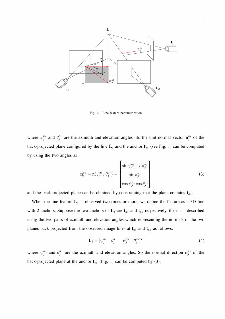
Fig. 1. Line feature parametrization

where ψa1j and θa1j are the azimuth and elevation angles. So the unit normal vector na1

j of the

back-projected plane configured by the line Lj and the anchor ta1 (see Fig. 1) can be computed

by using the two angles as

na1j = n(ψa1

j , θa1j ) =

sinψa1

j cos θa1j

sin θa1j

cosψa1j cos θa1j

(3)

and the back-projected plane can be obtained by constraining that the plane contains ta1 .

When the line feature Lj is observed two times or more, we define the feature as a 3D line

with 2 anchors. Suppose the two anchors of Lj are ta1 and ta2 respectively, then it is described

using the two pairs of azimuth and elevation angles which representing the normals of the two

planes back-projected from the observed image lines at ta1 and ta2 as follows:

Lj = [ψa1j θa1j ψa2

j θa2j ]T (4)

where ψa2j and θa2j are the azimuth and elevation angles. So the normal direction na2

j of the

back-projected plane at the anchor ta2 (Fig. 1) can be computed by (3).

9

C. Anchors Selection for the Line Parametrization

After two observations, the line feature will be fully initialized. Note that in this paper, “fully

initialized” simply means it is observed at least twice. It does not mean an accurate 3D location

can be estimated from these two measurements. So even when the parallax for a particular line

(the angle between the planes) is not large enough to calculate the 3D location, the initialization

of the line features in the state vector is still accurate due to the new parametrization we used.

If a line feature is observed more than twice, two of the camera centres are needed to be

chosen as the anchors. A simple strategy for anchor selection is to define the two anchors as the

camera centres from which Lj is observed for the first and second time. When we reproject the

3D line feature into the image from any other viewpoint, we use the same geometry constraint

as trifocal tensor [18]. The main idea is that all three back-projected planes intersect at the 3D

line feature, making it possible to use the two anchored back-projected planes to represent the

third one. So at most two of the three planes are linearly independent.

When the motion of the camera does not gain enough parallax for a particular line, which

means all the three back-projected planes are nearly the same, any two camera centres can be

selected as anchors. In this case, when projecting the line feature from the camera pose which is

not one of the anchors, the projective function is still correct since it uses the linear combination

of the same two planes to represent the same third plane. However, if the two back-projected

planes at the two anchors are the same, but the third one is different, there will be an issue because

it is impossible to use linear combination of the same two planes to represent a different plane.

In practice, this can cause problem when the two back-projected planes at the two anchors are

close to be the same. Therefore anchors need to be selected to avoid this situation.

In this paper, the strategy proposed for selecting the anchors is the following. We first define

the anchors as the camera centres where Lj is observed for the first and second time. When the

feature is observed more than two times, we will compare the dot product of every two unit

normals of the back-projected planes which represent the cosine of the angle between every two

10

planes. We will choose the anchors such that the angle between the two anchored back-projected

planes is the closest to π/2 to avoid the above possible problem.

IV. BUNDLE ADJUSTMENT

While the proposed line feature parametrization can be used with an EKF based approach

to SLAM, the computational cost will be increased due to the presence of the previous camera

centres served as anchors within the state vector. On the other hand, no additional computational

cost is introduced in the optimization based approach such as BA where all the camera poses are

used as parameters. In this section, the observation function for BA using the new line feature

parametrization is first presented. Then the least squares optimization formulation for BA and

the initialization of features are briefly outlined.

A. Observation Function for BA

Suppose the line feature Lj is parametrized by [ψa1j θa1j ψa2

j θa2j ]T with the two anchors

ta1 and ta2 , respectively. The normalized image line lij projected from Lj at pi can be represented

as:

lij =lij√

(aij)2 + (bij)

2(5)

lij = [aij bij cij]T = K−TRi ni

j (6)

where nij is the normal of the back-projected plane of feature Lj at pi which can be computed

as

nij =

na1j = n(ψa1

j , θa1j ), if i = a1

na2j = n(ψa2

j , θa2j ), if i = a2

(ta2 − ti)Tna2j na1

j − (ta1 − ti)Tna1j na2

j , else

(7)

where na1j and na2

j are the unit vectors which represents the normals of the back-projected plane

of Lj at the two anchors ta1 and ta2 computed using (3). Ri and ti are the rotation matrix and

the translation vector of pi, respectively. K is the camera calibration matrix.

11

The first two equations in (7) are obvious. For the last equation of (7), an idea similar to trifocal

tensor [18] is used to compute the back-projected plane from the existing two back-projected

planes, and then project the plane to get the image line. The details are as follows.

First we transfer the origin of the world coordinates to ti. Suppose πij , π

a1j and πa2

j are the

three back-projected planes of Lj at ti, ta1 and ta2 , respectively. Since the image lines in the

three images are derived from the same line Lj , it follows that these three back-projected planes

are not independent but must intersect at this line in 3-space. This intersection constraint can

be expressed algebraically by the requirement that the 4× 3 matrix M = [πij πa1

j πa2j ] has at

most rank 2. The matrix M can be expressed by

M =

nij na1

j na2j

0 −(ta1 − ti)Tna1j −(ta2 − ti)Tna2

j

(8)

where nij is the normal of the back-projected plane at ti.

Now we can use πa1j and πa2

j to represent πij . And the normal ni

j can be computed as

nij = (ta2 − ti)Tna2

j na1j − (ta1 − ti)Tna1

j na2j . (9)

This is the last equation of (7).

The above observation function is equivalent to the observation function for Plucker coor-

dinates. Suppose the Plucker matrix Lj computed from the intersection of plane πa1j and πa2

j

is

Lj = πa2j (πa1

j )T − πa1j (πa2

j )T . (10)

So

[l14 l42 l34]T = (ta2 − ti)Tna2

j na1j − (ta1 − ti)Tna1

j na2j (11)

where li,j is the ith row and jth column element of Plucker matrix Lj .

As described in [18], [l14 l42 l34]T = [l∗23 l∗13 l

∗12]

T , where [l∗23 l∗13 l

∗12]

T are the elements from

the dual Plucker matrix L∗j computed by joining two points. [l∗23 l

∗13 l

∗12]

T is also the normal

vector nij of the plane back projected from ti [3]. This is equivalent to (9).

12

Using the observation function for Plucker coordinates in [3], the image line projected at ti

can be computed as

lij = K−TRi([l14 l42 l34]T − 0 × [l23 l13 l12]

T ) = K−TRi nij. (12)

This is equivalent to (6).

B. Objective Function and Least Squares Optimization

In the image, each image line consists of a set of edge points. So the objective function should

be the total square distances of these edge points to the reprojected image line computed from

the observation function, and should be minimized during the least squares optimization.

Suppose the observed image line projected from Lj at pi consists of a set of edge points

{xk}, k = 1 · · ·n where

xk = [uk vk 1]T (13)

with (uk, vk) be the image coordinate of the edge point.

The least squares optimization problem in BA is to minimize:

∥ξ∥2Σ−1

ij=∑ij

(εij)TΣ−1

ij (εij) (14)

where εij is the signed distance vector from the set of edge points {xk} to each reprojected image

line f(P) and Σij is the associated covariance matrix. εij can be computed by

εij = [ϵ1 · · · ϵk · · · ϵn]T = XTf(P) (15)

where

ϵk = xTk f(P) (16)

and

X = [x1 · · · xk · · · xn]. (17)

Here f is the observation function, P is the state vector and lij = f(P) is the reprojected image

line computed by using (5), (6) and (7).

13

1) Weight: In the least squares formulation (14), each signed distance vector is treated as an

observation. Now we use the uncertainty of the edge points to compute the uncertainty of this

observation.

Suppose the noises of uk and vk are nu, nv which are zero-mean Gaussian

nu ∼ N(0, δ2), nv ∼ N(0, δ2). (18)

Then the covariance matrix of xk is

Cxk = diag(δ2, δ2, 0). (19)

By (16) the variance of ϵk is

ωk = f(P)TCxkf(P). (20)

Because the reprojected image line f(P) has already been normalized in (5), we have

ωk = δ2. (21)

So the weight Σ−1ij in (14) is

Σ−1ij = [diag(ω1, · · · , ωk, · · · , ωn)]

−1 =1

δ2I. (22)

2) Linearization: For simplification, we omit the i and j which represent the pose ID and

feature ID respectively and only consider one term in (14). Suppose m is the iteration number

and Pm is the state vector estimated at the mth iteration, we assume that the observation function

f is linearized at Pm by

f(Pm +∆m+1m ) ≈ f(Pm) + JPm∆

m+1m (23)

where JPm is the linear mapping represented by the Jacobian matrix ∂f/∂P evaluate at Pm.

Substitute (23) into (15), we get

XTf(Pm +∆m+1m ) ≈ εm +XTJPm∆

m+1m (24)

14

where εm = XTf(Pm). Then the problem changes to minimize ∥εm+XTJPm∆m+1m ∥2Σ−1 , which

is a linear least squares problem. So the update ∆m+1m from the mth iteration to the (m + 1)th

iteration can be computed as

(XTJPm)TΣ−1(XTJPm)∆

m+1m = −(XTJPm)

TΣ−1εm. (25)

From (15), (22) and (25), we can get

JTPmEJPm∆

m+1m = −JT

PmEf(Pm) (26)

where E is a 3× 3 symmetric matrix which can be computed by

E = XXT =n∑

k=1

xkxTk . (27)

The information matrix of Pm can be computed by

IPm =1

δ2JT

PmEJPm . (28)

So we can see from (26) that no matter how many edge points specify the observed image line,

the computational cost will be almost the same during the least squares optimization because E

is a 3× 3 matrix which can be easily computed by (27).

C. Image Line Fitting

The observed image line lij consisting of the set of edge points {xk} can be fitted as the right

null-vector of the matrix A

A lij = 0 (29)

where A = E − ζ0W , W = diag(1, 1, 0), and ζ0 is the minimum root of the equation det(E −

ζW ) = 0 ([18]) computed as the smaller one of the non-infinity generalized eigenvalues of E.

15

D. Line Feature Initialization

If the line feature Lj is observed only once at pa1, then ta1 is its anchor and Lj can be

initialized as ψa1j = atan2(xa1j , z

a1j )

θa1j = atan2(ya1j ,√(xa1j )2 + (za1j )2)

(30)

na1j = [xa1j ya1j za1j ]T = (KRa1)

T la1j (31)

where la1j is the image line of Lj observed at pa1fitted by using (29).

If Lj is observed at least twice with anchors ta1 and ta2 , then the other two parameters

[ψa2j θa2j ]T can be initialized the same way as using (30) and (31).

It is clear that when using the proposed feature parametrization, the initial values of the line

feature parameters are always accurate even if the parallax is small.

V. LOCAL SUBMAP JOINING ALGORITHM

BA is computationally intractable for very large-scale problems no matter which feature

parametrization is used. Local map joining has shown to be an efficient strategy for large-

scale SLAM. Most of the existing map joining algorithms such as [9][19][20] are for joining

point features local maps and require the scale to be consistent among the local maps. In [21], a

map joining algorithm that can automatically determine the relative scale during the optimization

process is proposed. This section extends the map joining algorithm in [21] for joining the line

feature local maps.

A. Local Map Building

First step is to divide original data into groups to build local maps using BA with the new

line feature parametrization. The first pose in each of such groups is chosen as the origin of the

corresponding local map, [0 0 0 0 0 0]T . The last pose of the lth local map is selected as the

first pose of the (l + 1)th local map such that the local maps can be linked together.

16

When performing BA, at least 7 DoF, namely rotation, translation and scale should be fixed

[22]. The first pose defines the rotation and translation, while one more parameter is needed to fix

the scale. We choose the z value of the translation from the first pose to the second pose zLl2 for

this purpose. Typically this is the largest element in the translation vector tLl2 = [xLl2 yLl2 zLl2]T .

Setting zLl2 = 1 defines the scale of the local map.

B. Deleting Features and Poses from Local Maps

It is unnecessary to include all the poses and features of the local maps in the state vector for

map joining because only part of the poses and features in local maps contain useful information

relating to the global map:

• “Common features” that appear in at least two local maps;

• The end pose of each local map;

• Translation of the second pose and all the anchors of the “common features”;

• Information matrix corresponding to all the above variables (computed using Schur com-

plement).

Here, the translation of the second pose is kept because it contains the scale of the local map

built by BA, and this scale needs to be present and used in the map joining process (see details

in Section V-C). Usually, the translation of the second pose is also an anchor for some features.

The map joining algorithm we proposed here follows the idea of [9], that is, using each local

map together with its information matrix as an integrated observation to update all the poses and

features involved in the global map. This is different from the hierarchical SLAM [23] where

each local map is treated as a fixed configuration and the global optimization only optimize the

coordinate frames of the local maps. Thus the common features appear in at least two local maps

contain important information for optimizing the global map. Removing the unnecessary features

and poses from the local maps as above will reduce the computational effort required in map

joining but will not affect the optimality of the global map. However if some of the common

17

features are also removed, then the map joining result will no longer be optimal although the

computational cost of map joining can be reduced further.

After removing the unnecessary elements, the lth local map can be represented as

[XLl ILl ] (32)

where XLl is the vector of all the kept poses and features, ILl is the information matrix for XL

l .

For the lth local map, XLl contains:

• The end pose pLle = [αL

le βLle γLle xLle yLle zLle]

T ;

• Common features LLlj observed in at least two local maps, include features [Lψa1

ljLθa1lj ]

T

observed only once and fully initialized 3D line features [Lψa1lj

Lθa1ljLψa2

ljLθa2lj ]

T in the lth

local map;

• Translation of the second pose and all the anchors of the kept line features. The ith translation

of the pose is denoted as tLli = [xLli yLli zLli ]T .

Here a local map may contain line features which are not fully initialized. However, in map

joining, only the common features that appear in at least two local maps are used (since the

features only appear in one local map does not contribute to the map joining result). So if a

feature is not fully initialized in one local map, it will be fully initialized in the map joining

since it will definitely appear in another local map.

C. Observation Function for Local Submap Joining

The n local maps [XLl ILl ], l = 1, · · · , n are treated as n observations in the map joining

process ([9]). The observation function for the map joining is given by

XL = H(XG) + w (33)

where

XL = [XL1 · · · XL

n ]T (34)

18

contains all the local maps as the observation. w is the noise of the observation and its covariance

matrix Σ is given by

Σ−1 = IL = diag(IL1 , · · · , ILn ). (35)

We use XG to denote the parameters in the global map. It contains the poses and line features

in the global coordinate frame which is the coordinate frame of the first local map. Comparing

with the observation XL, XG contains:

• pLle → pG

le = [αGle βG

le γGle xGle yGle zGle ]T

• {LLlj} → LG

j = [GψA1j

GθA1j

GψA2j

GθA2j ]T

• tLli → tGli = [xGli yGli zGli ]T .

(36)

There are two main differences between XL and XG:

(1) All the variables in the state vector XG are in the global coordinate frame which is the

coordinate frame of the first local map;

(2) {LLlj} → LG

j means all the features LLlj in different local maps representing the same feature

Lj will be one feature LGj in the global state vector. The anchor selection strategy described in

Section III-C is also used to avoid singularity in the observation function, so the anchors of line

features in the global map (with ID A1 and A2) may be different from the anchors in the local

maps. Note that part of features [Lψa1lj

Lθa1lj ]T which have been observed only once in one local

map, will be fully initialized 3D line features [GψA1j

GθA1j

GψA2j

GθA2j ]T in XG since they

are also observed in other local maps and thus have two anchors.

Here we use superscript G for the variables in the global coordinates and superscript L for

the variables in local map coordinates. Suppose l represents the local map ID, i represents the

pose translation ID, e represents the end pose of local map and j represents the feature ID. Let

A (A1 or A2) represents the global ID of the anchor of the line feature in the global map, while

a (a1 or a2) represents the local ID of the anchor of the feature in the local map. Then the

observation function XL = H(XG) can be written as follows:

19

The end pose of the (l − 1)th local map is the 1st pose of the lth local map. So the rotation

of the end pose of the lth local map, in the lth local map coordinates can be computed as

r (αLle, β

Lle, γ

Lle) = RG

le (RG(l−1)e)

T (37)

where RG(l−1)e and RG

le are the rotation matrices of the end pose of the (l − 1)th and lth local

map in global coordinates, respectively.

The translations of the 2nd, end pose and anchors of the lth local map, in the lth local map

coordinates can be computed as

tLli = RG(l−1)e (t

Gli − tG(l−1)e) / z

Ll2 (38)

where tGli is the ith translation of the lth local map, and tG(l−1)e is the translation of the end pose

of the (l − 1)th local map, all in global coordinates.

Here zLl2 in (38) is the relative scale between the local map and global map which is given in

[xLl2 yLl2 zLl2]T = RG

(l−1)e (tGl2 − tG(l−1)e) (39)

where tGl2 is the 2nd translation of the lth local map in global coordinates.

For the scale factor zLl2, when computing the ith translation in the lth local map in the lth local

map coordinates as tLli = RG(l−1)e (t

Gli − tG(l−1)e) by using the variables in the global state vector,

tLli is with the scale of the global map, however tLli in the observation vector is with the scale

of the lth local map. As we fix the z value of the second pose zLl2 = 1 when performing local

map BA, the lth local map is with the scale zLl2 = 1. So we can compute the 2nd translation of

the lth local map with the scale of the global map as (39). Thus the scale between global map

and the lth local map is zLl2 / zLl2 = zLl2 /1 = zLl2. Then tLli with the scale of the lth local map can

be computed as (38). The scale between different local maps will be optimized during the least

squares optimization process.

The pair of azimuth and elevation angles [Lψalj

Lθalj] of feature LLlj in the lth local map, in

20

the lth local map coordinates can be easily computed from the normal vector asLψa

lj = atan2(Lxalj,

Lzalj)

Lθalj = atan2(Lyalj,

√(Lxalj)

2 + (Lzalj)2) (40)

[LxaljLyalj

Lzalj]T = s Lna

lj. (41)

Here Lnalj is the vector which represents the normal of the back-projected plane of feature LL

lj

at anchor tGla in the lth local map, in the lth local map coordinates, given by

Lnalj =

RG

(l−1)eGnA

j , if a = A

RG(l−1)e

Gnalj, if a = A.

(42)

where GnAj is the unit vector which represents the normal of the back-projected plane of feature

LGj at anchor tGA in the global coordinates

GnAj = n(GψA

j ,GθAj ). (43)

Gnalj is the normal of the back-projected plane of feature LL

lj at anchor tGla in the lth local map,

in global coordinates and can be computed as

Gnalj = (tGA2

− tGla)T GnA2

jGnA1

j − (tGA1− tGla)

T GnA1j

GnA2j (44)

where GnA1j and GnA2

j represent the two normal vectors, tGA1and tGA2

represent the two anchors

of feature LGj in the global map, in the global coordinates. While tGla is the anchor of feature LL

lj

in the lth local map, in the global coordinates.

The details about the derivation of (44) are similar to that of observation function (7) described

in Section IV-A and are omitted here.

The s in (41) is a sign defined by

s =

+1, if Lφa

lj <= π/2

−1, if Lφalj > π/2

(45)

where Lφalj is the angle between vectors Lna

lj and Lnalj computed from the dot product

Lφalj = arccos

(Lna

lj ·Lna

lj

∥Lnalj∥

). (46)

21

Here Lnalj has the same physical meaning as Lna

lj but computed by the local map information

Lnalj = n(Lψa

lj,Lθalj) (47)

where [Lψa1lj

Lθa1lj ]T is from the measurement vector XL.

Here the sign s is used to make the observation function, measurement vector and the

information matrix consistent. As we know, both ±Lnalj represents the normal of the same

back-projected plane. So for the line feature parametrization proposed in this paper, there are

4 choices of each line feature. This is similar to the orthonormal representation in [6] because

(±U,±W ) represent the same Plucker line. In BA, this doesn’t matter because BA will converge

to one (out of four) correct solution depending on the initial guess. However in the map joining,

the normal computed using the observation function must be the same choice as the one in the

measurement vector because the local map information matrix obtained through BA is about

the particular choice from the BA result. So we first compare the two normal vectors computed

from the observation function and the measurement vector, respectively. If the angle between

these two normals are more than π/2, the normal computed from the observation function must

be in the opposite direction and thus we define the sign s = −1.

D. Least Squares Optimization of Map Joining

Local submap joining for line feature monocular SLAM can now be stated as a least squares

problem similar to (14) such that

∥ε∥2Σ−1 = (H(XG)− XL)TΣ−1(H(XG)− XL) (48)

is minimized.

The measurement vector XL consists of all the local maps as shown in (34), the parameter

vector XG is the global map with all the kept poses and features in the global coordinates as

shown in (36), H(XG) is the observation function in (33), and Σ−1 is given in (35), which is

the combination of the information matrices of all the local maps.

22

E. Initialization for Local Submap Joining Algorithm

To join the lth local map into global map, all the variables in the lth local map need to be

initialized in the global coordinates.

For the end pose and translations of anchors,

r (αGle, β

Gle , γ

Gle) = RL

le RG(l−1)e (49)

tGli = (RG(l−1)e)

T tLli + tG(l−1)e. (50)

For the pose initialization, we simply assume the relative scale between local map and global

map is equal to 1 and let the map joining algorithm adjust the relative scale.

Line features not already present in the global map, can be initialized by

n(GψAj ,

GθAj ) = (RG(l−1)e)

T n(Lψalj,

Lθalj) (51)

with the two anchors A1 = a1 and A2 = a2.

If the 3D line feature has already been included in the global map, an anchor changed

initialization similar to Section III-C is done to avoid using the linear combination of the same

two back-projected planes to represent a different plane in (44). After the anchors are defined,

the initialization is the same as using (51).

F. Computational Complexity

As described in [24], suppose there are OG feature projections as observations from CG poses.

If (26) is solved by Schur complement U W

W T V

∆P

∆F

=

EP

EF

(52)

(U −WV −1W T )∆P = EP −WV −1EF (53)

V∆F = EF −W T∆P , (54)

23

then the computational complexity of one iteration for the global BA is Θ(OG +OGCG +C3G),

where the computational complexity of computing information matrix JTPmEJPm is proportional

to the number of the observations Θ(OG), Θ(OGCG) is the computational complexity of com-

puting the product WV −1W T , and the computational complexity of solving the linear system

(53) is Θ(C3G) [8].

For the map joining algorithm, the computational cost consists of two parts: building the local

maps and joining the local maps.

Suppose the observations are equally divided to build n local maps. In each local map, there are

CL camera poses and OL feature projections as observations, with CG = n×CL and OG = n×OL.

So the computational complexity of building n local maps is Θ(OL + OLCL + C3L) × n =

Θ(OG + 1nOGCG + 1

n2C3G). Obviously the computational complexity of building n local maps is

much less than that of a global BA.

For the map joining process, suppose OM variables are kept from different local maps in

(34) as observations, and in the global map there are CM camera poses or translations. Similar

to BA, the computational complexity of computing information matrix is Θ(OM). For building

the Schur complement, the nonzero elements in each column of matrix W only appear at the

two anchors of this corresponding feature in each local map, as well as the first poses of these

local maps. So the number of nonzero elements in matrix is also the same as the observations

OM , thus the computational complexity of computing WV −1W T is Θ(OMCM). In the global

map, besides n end poses with full rotation and translation, all the other kept poses are only

translations. Thus the computational complexity of solving the linear system depending on the

number of poses is Θ(18C3

M). So for the map joining process, the computational complexity is

Θ(OM +OMCM + 18C3

M).

The overall computational complexity of the map joining algorithm is Θ(OG + 1nOGCG +

1n2C

3G +OM +OMCM + 1

8C3

M).

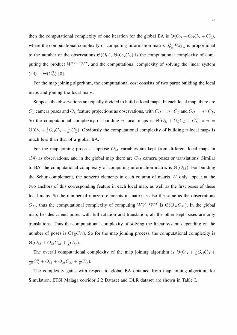
The complexity gains with respect to global BA obtained from map joining algorithm for

Simulation, ETSI Malaga corridor 2.2 Dataset and DLR dataset are shown in Table I.

24

TABLE I

COMPUTATIONAL COMPLEXITY GAIN OBTAINED FROM MAP JOINING IN COMPARISON WITH GLOBAL BA

Dataset OG or OL CG or CL n OM CM gain

SimulationGlobal BA 1763 76 1

Map joining 440 20 4 328 73 5

MalagaGlobal BA 2880 240 1

Map joining 960 81 3 127 75 19

DLRGlobal BA 18950 3298 1

Map joining 4780 825 4 1093 626 15

For the same dataset, the number and size of local maps also affect the computational

complexity of the map joining algorithm. Choosing the suitable number of local maps to minimize

the overall computational cost is another interesting research topic [25] and is not discussed here.

VI. SIMULATION AND EXPERIMENTAL RESULTS

Simulation and real datasets have been used to check the validity and accuracy of the BA and

map joining algorithms using the proposed line feature parametrization.

A. Simulation Results

The environment is set up as a 11m × 11m square corridor with 11m length (10m length

inside and 12m length outside), 2m width and 3m high each side (Fig. 2). Besides the 4×4 = 16

lines located at the intersection of ceiling and wall (or floor and wall) along the corridor, lines

of 1m length in every 1m are simulated on the floor and ceiling. And 2m length lines every

1m are simulated on the right and left walls. All the lines on the floor, ceiling and walls are

perpendicular to the length direction of the corridor. A 0.3m × 0.3m × 0.3m box and a 1m ×

25

!"#$

%!"#$&!"#$

Fig. 2. Simulation environment and robot trajectory

0.5m × 1.5m cabinet are also simulated in each side of the corridor. There are totally 296 lines

in the simulation environment.

The robot is simulated as moving in the middle of the corridor with 1m distance each step

when moving straight forward, and 0.25m distance and π/16 rad each step when turning at the

corner. There are 76 poses on the square trajectory in total. The camera onboard the robot is

assumed to be 0.5m above the ground and look forward. The simulation environment and the

trajectory are shown in Fig. 2.

All the lines are projected in the images using the pinhole camera model. The camera is

modelled as [−π/4, π/4] of FOV, [0, +∞] observation distance, 800 × 800 image resolution,

[400, 400] principle point and [400, 400] focal length, as described in Table II. The lines are

sampled as edge points with constant distance 1 pixel along the line direction. A random Gaussian

noise with σ = 1 is added on the theoretical image coordinates of the edge points within the

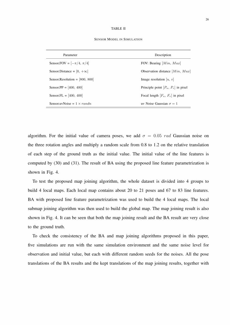
FOV as the observations of the 3D line features. Typical simulated images are shown in Fig. 3.

The simulated image lines in all the 76 simulated images are used in the proposed BA

26

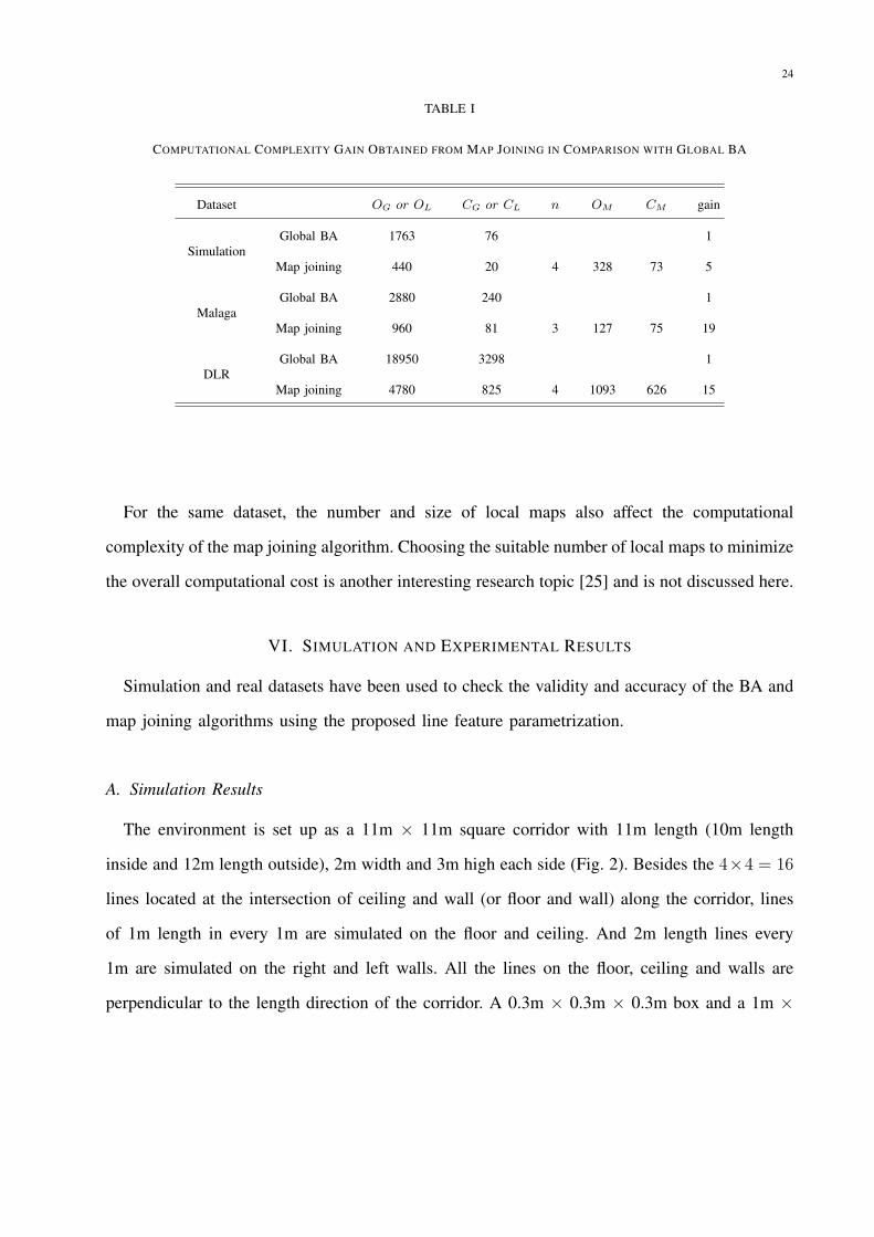
TABLE II

SENSOR MODEL IN SIMULATION

Parameter Description

Sensor.FOV = [−π/4, π/4] FOV: Bearing [Min, Max]

Sensor.Distance = [0, +∞] Observation distance [Min, Max]

Sensor.Resolution = [800, 800] Image resolution [u, v]

Sensor.PP = [400, 400] Principle point [Pu, Pv] in pixel

Sensor.FL = [400, 400] Focal length [Fu, Fv] in pixel

Sensor.uvNoise = 1× randn uv Noise Gaussian σ = 1

algorithm. For the initial value of camera poses, we add σ = 0.05 rad Gaussian noise on

the three rotation angles and multiply a random scale from 0.8 to 1.2 on the relative translation

of each step of the ground truth as the initial value. The initial value of the line features is

computed by (30) and (31). The result of BA using the proposed line feature parametrization is

shown in Fig. 4.

To test the proposed map joining algorithm, the whole dataset is divided into 4 groups to

build 4 local maps. Each local map contains about 20 to 21 poses and 67 to 83 line features.

BA with proposed line feature parametrization was used to build the 4 local maps. The local

submap joining algorithm was then used to build the global map. The map joining result is also

shown in Fig. 4. It can be seen that both the map joining result and the BA result are very close

to the ground truth.

To check the consistency of the BA and map joining algorithms proposed in this paper,

five simulations are run with the same simulation environment and the same noise level for

observation and initial value, but each with different random seeds for the noises. All the pose

translations of the BA results and the kept translations of the map joining results, together with

27

0 100 200 300 400 500 600 700 800

0

100

200

300

400

500

600

700

800

(a) Moving straight forward

0 100 200 300 400 500 600 700 800

0

100

200

300

400

500

600

700

800

(b) Turning

Fig. 3. Simulated images

−2 0 2 4 6 8 10 12 14−2

0

2

4

6

8

10

12

X (m)

Z (

m)

Ground Truth

Initial Value

Bundle Adjustment

Map Joining

BA_OR_1

Fig. 4. BA and map joining results of simulation

28

TABLE III

CONSISTENCY OF BA RESULT BY NEES CHECK (95%)

Run 1 2 3 4 5

Dimensions 224 224 224 224 224

H Bound 267.35 267.35 267.35 267.35 267.35

NEES 205.27 249.17 191.15 210.24 207.72

L Bound 184.44 184.44 184.44 184.44 184.44

TABLE IV

CONSISTENCY OF MAP JOINING RESULT BY NEES CHECK (95%)

Run 1 2 3 4 5

Dimensions 209 209 215 209 215

H Bound 250.93 250.93 257.50 250.93 257.50

NEES 218.03 232.67 224.11 254.92 208.53

L Bound 170.86 170.86 176.28 170.86 176.28

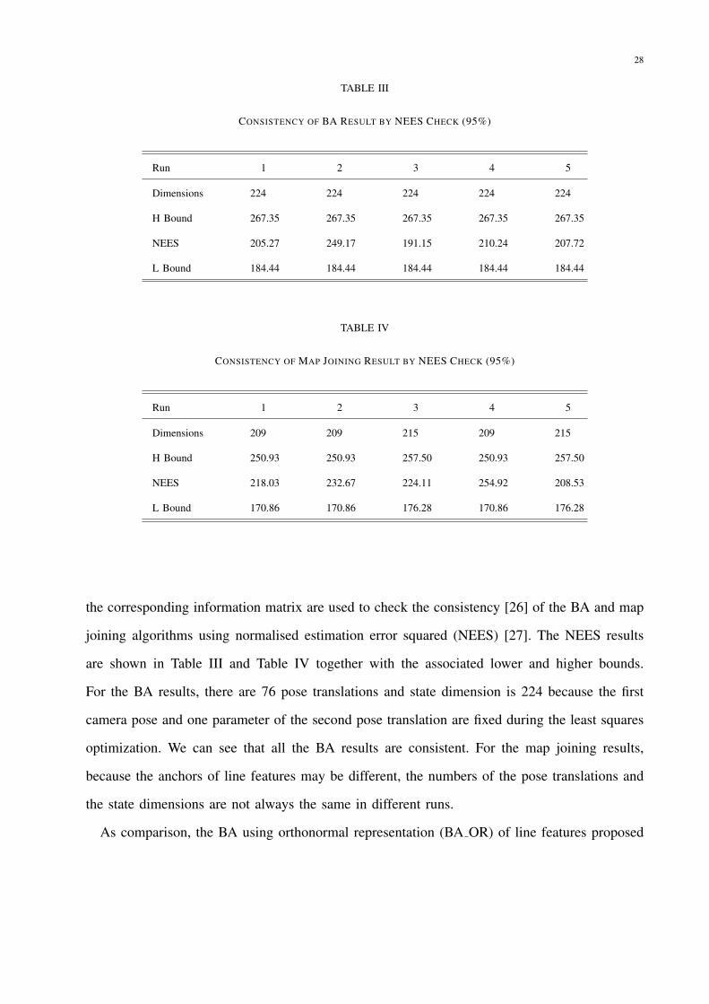
the corresponding information matrix are used to check the consistency [26] of the BA and map

joining algorithms using normalised estimation error squared (NEES) [27]. The NEES results

are shown in Table III and Table IV together with the associated lower and higher bounds.

For the BA results, there are 76 pose translations and state dimension is 224 because the first

camera pose and one parameter of the second pose translation are fixed during the least squares

optimization. We can see that all the BA results are consistent. For the map joining results,

because the anchors of line features may be different, the numbers of the pose translations and

the state dimensions are not always the same in different runs.

As comparison, the BA using orthonormal representation (BA OR) of line features proposed

29

in [6] is implemented and compared with the BA proposed in this paper using the simulation

dataset described above. The camera pose parametrization for the BA OR is the same as (1)

proposed in this paper. And we also use E matrix in (27) instead of the two weighted points

[6][18] in the objective function in order to compare with the proposed BA using the same

mean square error (MSE) (the objective function defined in (14) divided by the number of line

observations).

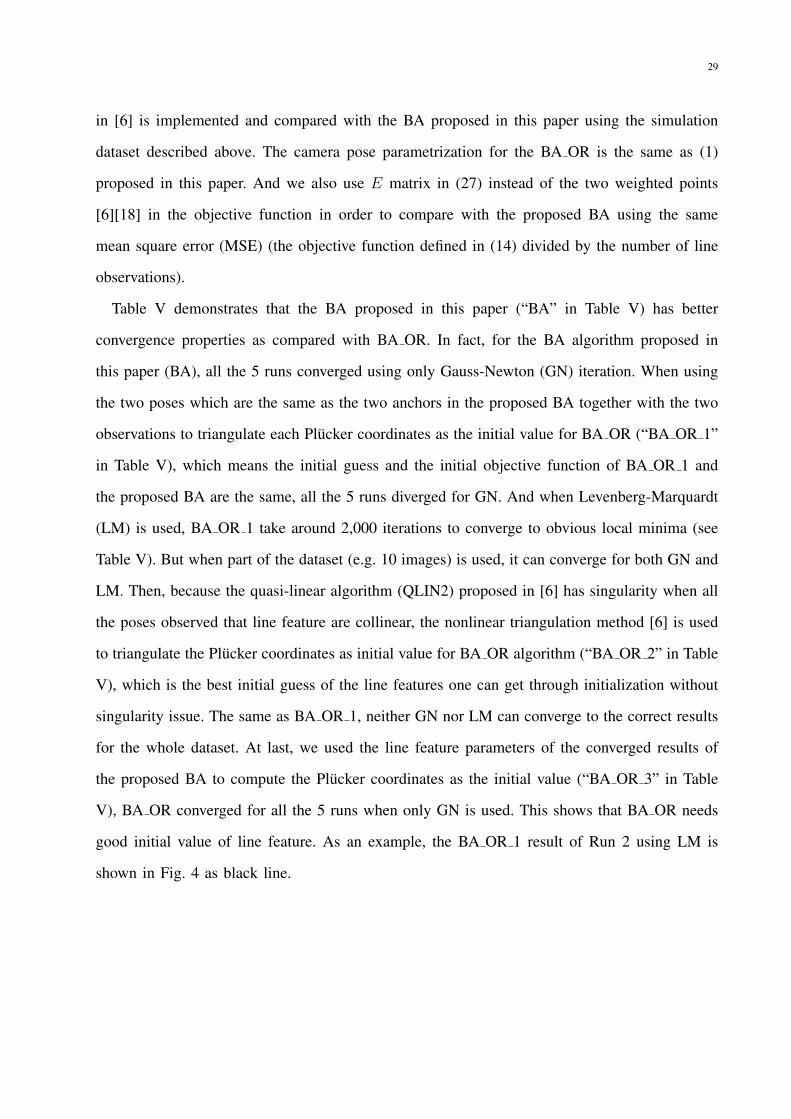
Table V demonstrates that the BA proposed in this paper (“BA” in Table V) has better

convergence properties as compared with BA OR. In fact, for the BA algorithm proposed in

this paper (BA), all the 5 runs converged using only Gauss-Newton (GN) iteration. When using

the two poses which are the same as the two anchors in the proposed BA together with the two

observations to triangulate each Plucker coordinates as the initial value for BA OR (“BA OR 1”

in Table V), which means the initial guess and the initial objective function of BA OR 1 and

the proposed BA are the same, all the 5 runs diverged for GN. And when Levenberg-Marquardt

(LM) is used, BA OR 1 take around 2,000 iterations to converge to obvious local minima (see

Table V). But when part of the dataset (e.g. 10 images) is used, it can converge for both GN and

LM. Then, because the quasi-linear algorithm (QLIN2) proposed in [6] has singularity when all

the poses observed that line feature are collinear, the nonlinear triangulation method [6] is used

to triangulate the Plucker coordinates as initial value for BA OR algorithm (“BA OR 2” in Table

V), which is the best initial guess of the line features one can get through initialization without

singularity issue. The same as BA OR 1, neither GN nor LM can converge to the correct results

for the whole dataset. At last, we used the line feature parameters of the converged results of

the proposed BA to compute the Plucker coordinates as the initial value (“BA OR 3” in Table

V), BA OR converged for all the 5 runs when only GN is used. This shows that BA OR needs

good initial value of line feature. As an example, the BA OR 1 result of Run 2 using LM is

shown in Fig. 4 as black line.

30

TABLE V

CONVERGENCE AND MSE OF SIMULATION

BA BA OR 1 BA OR 2 BA OR 3

Run GN GN LM GN LM GN

1 199.2081 N 1389.0838 N 1810.6741 199.2081

2 199.6360 N 622.8728 N 1345.6028 199.6360

3 199.5360 N 749.8807 N 2715.6562 199.5360

4 199.8054 N 2364.5208 N 2328.5485 199.8054

5 199.2762 N 888.2551 N 991.8803 199.2762

B. Results using Real Experimental Datasets

For the experimental results, the dataset collected ourselves (FEIT UTS Corridor Dataset) and

publicly available datasets (ETSI Malaga corridor 2.2 Dataset [28] and DLR Dataset [29]) are

used for the algorithms described in this paper. All the datasets are corridor environment because

this kind of environment is mainly described by the line features.

1) FEIT UTS Corridor Dataset: For the first experimental result, the dataset is collected in the

corridor of level 6, building 2 at University of Technology, Sydney (UTS). The Dragonfly DR2-

HIBW/HICOL-XX camera is used to capture the images and the image resolution is 1024×768.

The calibration is done by using the Matlab Automatic Camera Calibration Toolbox [30]. Then

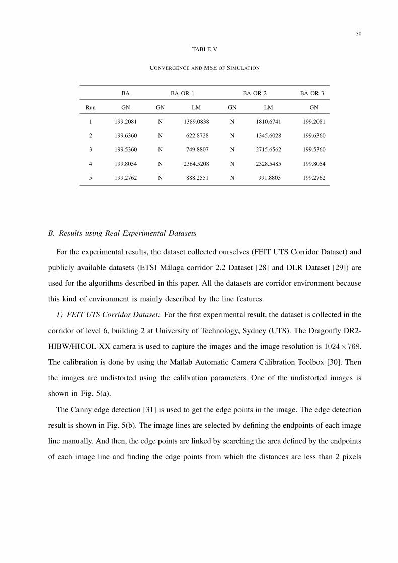
the images are undistorted using the calibration parameters. One of the undistorted images is

shown in Fig. 5(a).

The Canny edge detection [31] is used to get the edge points in the image. The edge detection

result is shown in Fig. 5(b). The image lines are selected by defining the endpoints of each image

line manually. And then, the edge points are linked by searching the area defined by the endpoints

of each image line and finding the edge points from which the distances are less than 2 pixels

31

(a) Original image (b) Edge detection

(c) Edge linking (d) Image line

Fig. 5. Image line detection results for FEIT UTS Corridor Dataset

to the image line defined by the endpoints. The image line linking result is shown in Fig. 5(c)

and Fig. 5(d).

The BA with proposed line feature parametrization is implemented using 14 images taken

from one end to the other of the corridor involving 31 line features. For comparison, the BA

using point features is also performed based on the SIFT feature extraction and matching, multi-

level RANSAC and parallax angle feature parametrization as described in [21]. There are 6150

point features and the mean square error of the reprojections converged to 0.5967. So we believe

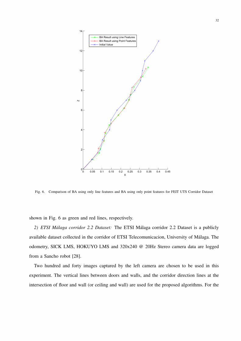
the result of BA using point features is reasonable and use it as the benchmark. The BA result

using proposed line feature parametrization and the BA result by using the point features are

32

! " !# !#" !$ !$" !% !%" !& !&"

$

&

'

(

#

#$

#& )

)

*+),-./01)/.234)523-)6-71/8-.

*+),-./01)/.234)9:231)6-71/8-.

;321270)<70/-

=)

>)

Fig. 6. Comparison of BA using only line features and BA using only point features for FEIT UTS Corridor Dataset

shown in Fig. 6 as green and red lines, respectively.

2) ETSI Malaga corridor 2.2 Dataset: The ETSI Malaga corridor 2.2 Dataset is a publicly

available dataset collected in the corridor of ETSI Telecomunicacion, University of Malaga. The

odometry, SICK LMS, HOKUYO LMS and 320x240 @ 20Hz Stereo camera data are logged

from a Sancho robot [28].

Two hundred and forty images captured by the left camera are chosen to be used in this

experiment. The vertical lines between doors and walls, and the corridor direction lines at the

intersection of floor and wall (or ceiling and wall) are used for the proposed algorithms. For the

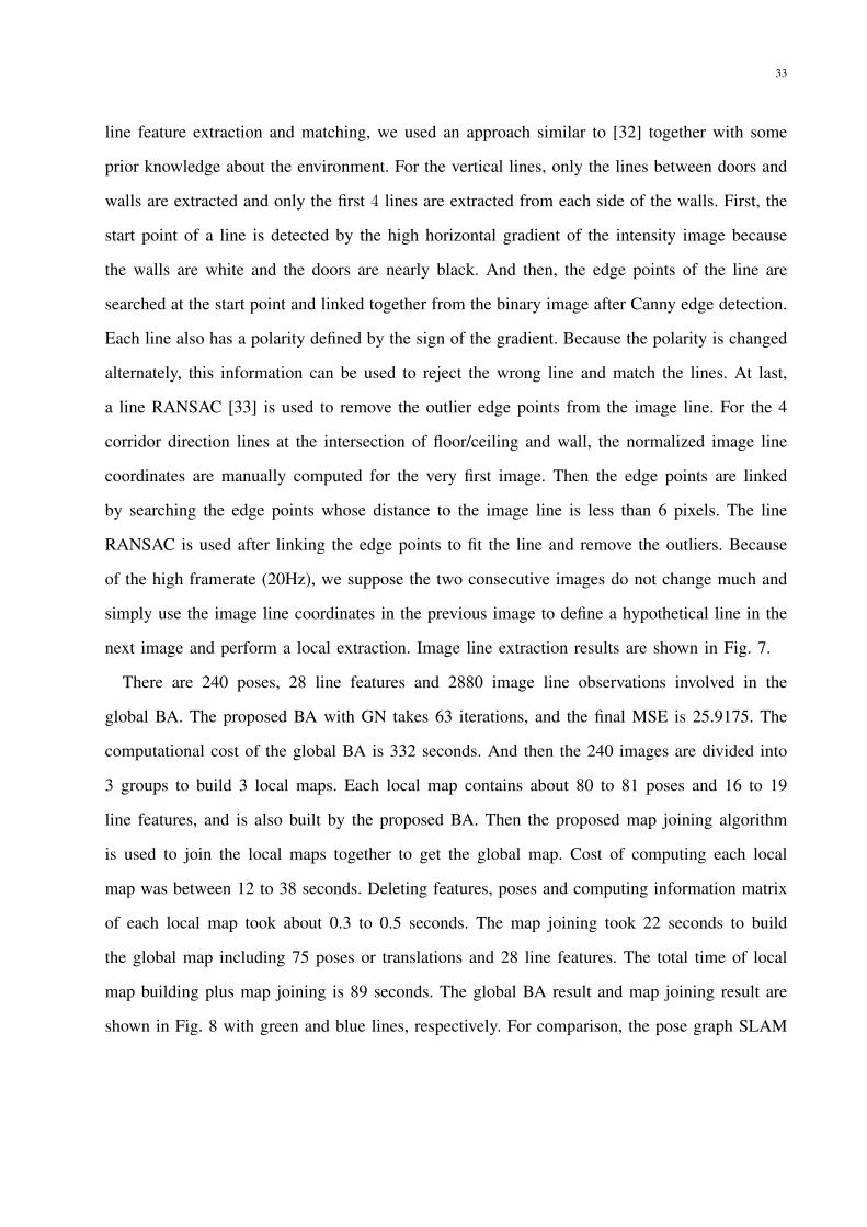
33

line feature extraction and matching, we used an approach similar to [32] together with some

prior knowledge about the environment. For the vertical lines, only the lines between doors and

walls are extracted and only the first 4 lines are extracted from each side of the walls. First, the

start point of a line is detected by the high horizontal gradient of the intensity image because

the walls are white and the doors are nearly black. And then, the edge points of the line are

searched at the start point and linked together from the binary image after Canny edge detection.

Each line also has a polarity defined by the sign of the gradient. Because the polarity is changed

alternately, this information can be used to reject the wrong line and match the lines. At last,

a line RANSAC [33] is used to remove the outlier edge points from the image line. For the 4

corridor direction lines at the intersection of floor/ceiling and wall, the normalized image line

coordinates are manually computed for the very first image. Then the edge points are linked

by searching the edge points whose distance to the image line is less than 6 pixels. The line

RANSAC is used after linking the edge points to fit the line and remove the outliers. Because

of the high framerate (20Hz), we suppose the two consecutive images do not change much and

simply use the image line coordinates in the previous image to define a hypothetical line in the

next image and perform a local extraction. Image line extraction results are shown in Fig. 7.

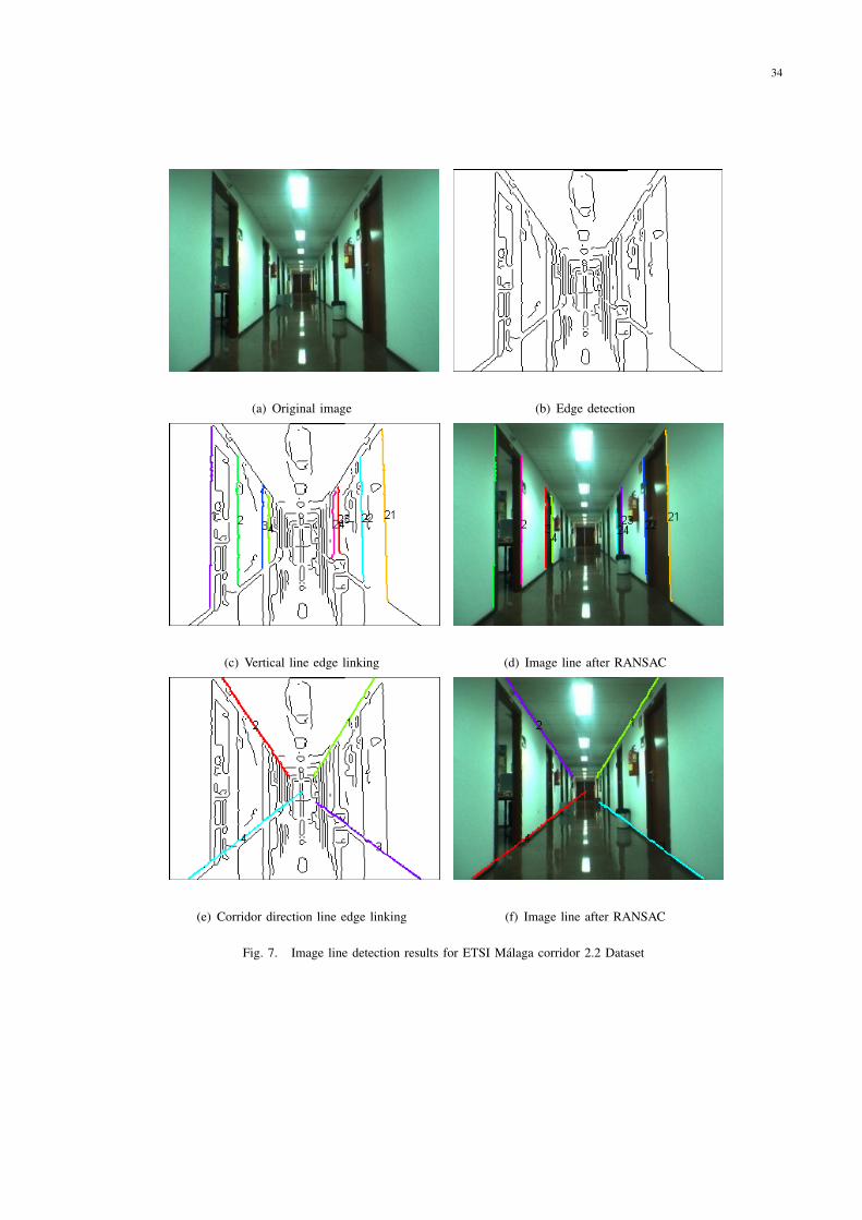
There are 240 poses, 28 line features and 2880 image line observations involved in the

global BA. The proposed BA with GN takes 63 iterations, and the final MSE is 25.9175. The

computational cost of the global BA is 332 seconds. And then the 240 images are divided into

3 groups to build 3 local maps. Each local map contains about 80 to 81 poses and 16 to 19

line features, and is also built by the proposed BA. Then the proposed map joining algorithm

is used to join the local maps together to get the global map. Cost of computing each local

map was between 12 to 38 seconds. Deleting features, poses and computing information matrix

of each local map took about 0.3 to 0.5 seconds. The map joining took 22 seconds to build

the global map including 75 poses or translations and 28 line features. The total time of local

map building plus map joining is 89 seconds. The global BA result and map joining result are

shown in Fig. 8 with green and blue lines, respectively. For comparison, the pose graph SLAM

34

(a) Original image (b) Edge detection

(c) Vertical line edge linking (d) Image line after RANSAC

(e) Corridor direction line edge linking (f) Image line after RANSAC

Fig. 7. Image line detection results for ETSI Malaga corridor 2.2 Dataset

35

0 2 4 6 8 10 12−1

−0.5

0

0.5

1

1.5

X (m)

Y (

m)

ICP+PoseGraphBundle AdjustmentMap Joining

Fig. 8. BA, map joining and pose graph SLAM results of ETSI Malaga corridor 2.2 Dataset

result based on ICP using the backward 2D laser scans is also shown in Fig. 8 with red line,

which is arguably the best result one can achieve in this kind of environment. BA OR algorithm

is also implemented. When GN is used, both BA OR 1 and BA OR 2 directly diverged. And

when LM is used, both BA OR 1 and BA OR 2 converge to the same MSE as 25.9175. While

the iteration numbers are 488 and 481, respectively.

The 3D line features are reprojected to the image lines in different images using the estimated

poses and line features obtained though BA and computed by the observation function proposed

in this paper. The image line reprojection results for two randomly selected images (image 1

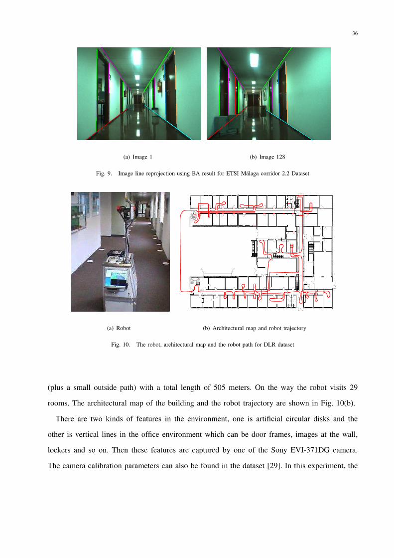
and image 128, endpoints are manually given) are shown in Fig. 9.

3) DLR Dataset: Another large-scale publicly available dataset with multiple loops is also

used to test the BA and map joining algorithms proposed in this paper. The dataset was recorded

at a corridor environment in the DLR (Deutsches Zentrum fur Luft und Raumfahrt), Institute of

Robotics and Mechatronics building by a mobile robot (Fig. 10(a)). So it is also a line structured

environment and ideal for the proposed SLAM algorithms. As described in [29], the building

covers a region of 60m×45m and the robot path consists of three large loops within the building

36

(a) Image 1 (b) Image 128

Fig. 9. Image line reprojection using BA result for ETSI Malaga corridor 2.2 Dataset

(a) Robot (b) Architectural map and robot trajectory

Fig. 10. The robot, architectural map and the robot path for DLR dataset

(plus a small outside path) with a total length of 505 meters. On the way the robot visits 29

rooms. The architectural map of the building and the robot trajectory are shown in Fig. 10(b).

There are two kinds of features in the environment, one is artificial circular disks and the

other is vertical lines in the office environment which can be door frames, images at the wall,

lockers and so on. Then these features are captured by one of the Sony EVI-371DG camera.

The camera calibration parameters can also be found in the dataset [29]. In this experiment, the

37

Fig. 11. Line features data association in DLR dataset

vertical line features are used in the proposed BA and map joining algorithms. Feature extraction

and data association results are given in the dataset (Fig. 11). Because there is no line features

along the outside path of the robot trajectory, the odometry is needed in BA to deal with the

lack of information.

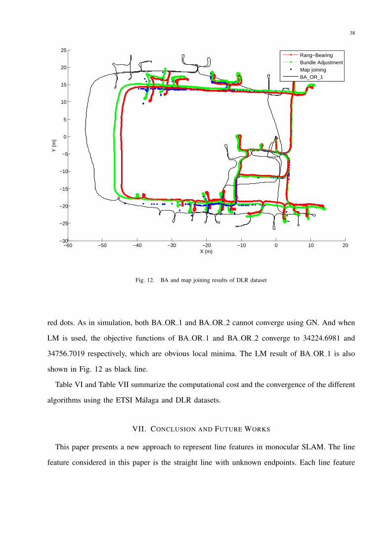
There are 3298 poses, 1206 3D line features, 15653 image line observations and 3297 odometry

observations in total. The proposed BA algorithm takes 853 seconds to get the global BA result.

The final objective function is 3024.6731 (Here we use objective function instead of MSE because

the odometry is involved). The global BA result is shown in Fig. 12 as green dots. Then the

whole dataset is divided into 4 groups to build 4 local maps. Each local map contains about 825

to 826 poses and 295 to 412 line features. The local maps are first built by the BA proposed in

this paper, and then the proposed map joining algorithm is used to join the local maps together to

get the global map. Cost of computing each local map was between 18 to 31 seconds. Deleting

features, poses and computing information matrix of each local map took about 11 to 20 seconds.

The map joining took 128 seconds to build the global map including 626 poses or translations

and 234 line features. The total time of local map building plus map joining is 286 seconds.

The map joining result is shown in Fig. 12 as blue dots. As the benchmark for comparison, the

range and bearing result using artificial circular disks as landmarks is also shown in Fig. 12 as

38

−60 −50 −40 −30 −20 −10 0 10 20−30

−25

−20

−15

−10

−5

0

5

10

15

20

25

X (m)

Y (

m)

Rang−BearingBundle AdjustmentMap joiningBA_OR_1

Fig. 12. BA and map joining results of DLR dataset

red dots. As in simulation, both BA OR 1 and BA OR 2 cannot converge using GN. And when

LM is used, the objective functions of BA OR 1 and BA OR 2 converge to 34224.6981 and

34756.7019 respectively, which are obvious local minima. The LM result of BA OR 1 is also

shown in Fig. 12 as black line.

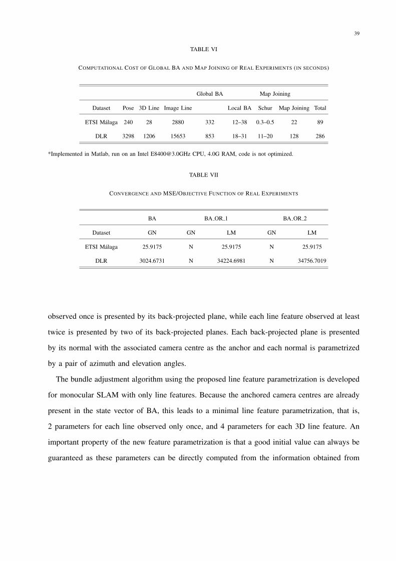
Table VI and Table VII summarize the computational cost and the convergence of the different

algorithms using the ETSI Malaga and DLR datasets.

VII. CONCLUSION AND FUTURE WORKS

This paper presents a new approach to represent line features in monocular SLAM. The line

feature considered in this paper is the straight line with unknown endpoints. Each line feature

39

TABLE VI

COMPUTATIONAL COST OF GLOBAL BA AND MAP JOINING OF REAL EXPERIMENTS (IN SECONDS)

Global BA Map Joining

Dataset Pose 3D Line Image Line Local BA Schur Map Joining Total

ETSI Malaga 240 28 2880 332 12–38 0.3–0.5 22 89

DLR 3298 1206 15653 853 18–31 11–20 128 286

*Implemented in Matlab, run on an Intel E8400@3.0GHz CPU, 4.0G RAM, code is not optimized.

TABLE VII

CONVERGENCE AND MSE/OBJECTIVE FUNCTION OF REAL EXPERIMENTS

BA BA OR 1 BA OR 2

Dataset GN GN LM GN LM

ETSI Malaga 25.9175 N 25.9175 N 25.9175

DLR 3024.6731 N 34224.6981 N 34756.7019

observed once is presented by its back-projected plane, while each line feature observed at least

twice is presented by two of its back-projected planes. Each back-projected plane is presented

by its normal with the associated camera centre as the anchor and each normal is parametrized

by a pair of azimuth and elevation angles.

The bundle adjustment algorithm using the proposed line feature parametrization is developed

for monocular SLAM with only line features. Because the anchored camera centres are already

present in the state vector of BA, this leads to a minimal line feature parametrization, that is,

2 parameters for each line observed only once, and 4 parameters for each 3D line feature. An

important property of the new feature parametrization is that a good initial value can always be

guaranteed as these parameters can be directly computed from the information obtained from

40

the measurement.

A map joining algorithm based on the proposed line feature parametrization is also presented.

Together with local maps built by BA, the algorithms are able to simultaneously optimize the

camera poses, feature positions and the relative scales. Simulation and experimental results

demonstrated the effectiveness and consistency of the proposed BA and map joining algorithms

using the new line feature parametrization.

Unlike the point features, robust line feature extraction and matching from image data still

remains a challenge. In the current experimental results shown in this paper, the line feature

matching involves some manual operations and prior knowledge of the line features. In the

next step, we are planning to improve the line feature extraction and matching algorithm such

that the proposed BA algorithm can be applied more robustly to general indoor environments.

Moreover, the relationship between the proposed line feature parametrization and the SP-Map

representation [34] needs further investigation. Monocular SLAM using both point features and

line features is straightforward by combining the point feature parametrization in [21] and the

line feature parametrization proposed in this paper.

REFERENCES

[1] A. J. Davison, “Real-time Simultaneous Localisation and Mapping with a Single Camera,” Proceedings of the International

Conference on Computer Vision (ICCV), vol. 2, pp. 1403-1410 (2003).

[2] G. Klein and D. Murray, “Improving the Agility of Keyframe-based SLAM,” Proceedings of the 10th European Conference

on Computer Vision (ECCV), Marseille, pp. 802-815 (2008).

[3] J. Sola, T.V. Calleja, J. Civera and J.M.M. Montiel, “Impact of landmark parametrization on monocular EKF-SLAM with

points and lines,” International Journal of Computer Vision, 97(3), 339-368 (2012).

[4] D. Simon and T.L. Chia, “Kalman Filtering with State Equality Constraints,” IEEE Transactions on Aerpspace and

Electronic Systems, 38(1), 128-136 (2002).

[5] S. J. Julier and J. J. LaViola, “On Kalman Filtering with Nonlinear Equality Constraints,” IEEE Transactions on Signal

Processing, 55(6), 2774-2784 (2007).

41

[6] A. Bartoli and P. Sturm, “Structure-from-motion using Lines: Representation, Triangulation and Bundle Adjustment,”

Computer Vision and Image Understanding, 100(3), 416-441 (2005).

[7] H. Strasdat, J. M. M. Montiel and A. J. Davison, “Real-time Monocular SLAM: Why Filter?” Proceedings of the IEEE

International Conference on Robotics and Automation (ICRA), Anchorage, USA, pp. 2657-2664 (May 2010).

[8] K. Konolige and M. Agrawal, “FrameSLAM: From Bundle Adjustment to Real-Time Visual Mapping,” IEEE Transactions

on Robitics, 24(5), 1066-1077 (Oct. 2008).

[9] S. Huang, Z. Wang and G. Dissanayake, “Sparse Local Submap Joining Filter for Building Large-Scale Maps,” IEEE

Transactions on Robotics, 24(5), 1121-1130 (Oct. 2008).

[10] E. Eade and T. Drummond, “Edge Landmarks in Monocular SLAM,” Image and Vision Computing, 27, 588-596 (2009).

[11] G. Klein and D. Murray, “Full-3D Edge Tracking with A Particle Filter,” Proceedings of the British Machine Vision

Conference (BMVC), Edinburgh, vol. 3, pp. 1119-1128 (2006).

[12] P. Smith, I. Reid and A. J. Davison, “Real-time Monocular SLAM with Straight Lines,” Proceedings of the British Machine

Vision Conference (BMVC), Edinburgh, vol. 1, pp. 17-26 (2006).

[13] A. P. Gee and W. Mayol-Cuevas, “Real-Time Model-Based SLAM using Line Segments,” 2nd International Symposium

on Visual Computing, vol. 4292, pp. 354-363 (Nov. 2006).

[14] C. J. Taylor and D. J. Kriegman, “Structure and Motion from Line Segments in Multiple Images,” IEEE Transactions on

Pattern Analysis and Machine Intelligence, 17(11), 1021-1032 (1995).

[15] T. Lemaire and S. Lacroix, “Monocular-vision Based SLAM using Line Segments,” Proceedings of the IEEE International

Conference on Robotics and Automation (ICRA), Rome, Italy, pp. 2791-2796 (2007).

[16] J. Sola, T. Vidal-Calleja and M. Devy, “Undelayed Initialization of Line Segments in Monocular SLAM,” Proceedings of

the IEEE/RSJ International Conference on Intelligent Robots and Systems (IROS), Saint Louis, USA, pp. 1553-1558 (Oct.

2009).

[17] T. Vidal-Calleja, C. Berger, J. Sola and S. Lacroix. “Large Scale Multiple Robot Visual Mapping with Heterogeneous

Landmarks in Semi-Structured Terrain,” Robotics and Autonomous Systems, 59, 654-674 (2011).

[18] R. Hartley and A. Zisserman, “Multiple View Geometry in Computer Vision,” 2nd Ed., (Cambridge University Press,

2003).

[19] G. Hu, S. Huang and G. Dissanayake, “3D I-SLSJF: A Consistent Sparse Local Submap Joining Algorithm for Building

Large-Scale 3D Maps,” Proceedings of the 48th IEEE Conference on Decision and Control, Shanghai, China, pp. 6040-6045

(2009).

[20] L. Zhao, S. Huang, L. Yan, J. Wang, G. Hu and G. Dissanayake, “Large-Scale Monocular SLAM by Local Bundle

42

Adjustment and Map Joining,” Proceedings of the 11th International Conference on Control, Automation, Robotics and

Vision (ICARCV), Singapore, pp. 431-436 (Dec. 2010).

[21] L. Zhao, S. Huang, L. Yan and G. Dissanayake, “Parallax Angle Parametrization for Monocular SLAM,” Proceedings of

the IEEE International Conference on Robotics and Automation (ICRA), Shanghai, China, pp. 3117-3124 (May 2011).

[22] H. Strasdat, J. M. M. Montiel and A. J. Davison, “Scale Drift-Aware Large Scale Monocular SLAM,” Proceedings of the

Robotics: Science and Systems Conference (RSS) (2010).

[23] C. Estrada, J. Neira and J.D. Tardos. “Hierarchical SLAM: Real-time Accurate Mapping of Large Environments,” IEEE

Transactions on Robotics, 21(4), pp. 588-596 (2005).

[24] E. Mouragnon, M. Lhuillier, M. Dhome, F. Dekeyser and P. Sayd, “Generic and Real Time Structure from Motion using

Local Bundle Adjustment,” Image and Vision Computing, 27(8), 1178-1193 (2009).

[25] L. M. Paz and J. Neira, “Optimal Local Map Size for EKF-based SLAM,” Proceedings of the IEEE/RSJ International

Conference on Intelligent Robots and Systems (IROS), Beijing, China, pp. 9-15 (Oct. 2006).

[26] S. Huang and G. Dissanayake, “Convergence and Consistency Analysis for Extended Kalman Filter Based SLAM,” IEEE

Transactions on Robotics, 23(5), 1036-1049 (2007).

[27] S. Huang, Z. Wang, G. Dissanayake and U. Frese, “Iterated D-SLAM Map Joining: Evaluating Its Performance in Terms

of Consistency, Accuracy and Efficiency,” Autonomous Robots, 27, 409-429 (2009).

[28] J. L. Blanco, “Mobile Robot Programming Toolkit (MRPT),” [Online]. Available: http://www.mrpt.org/node/239/.

[29] J. Kurlbaum and U. Frese, “A Benchmark Data Set for Data Association,” [Online]. Available: http://www.sfbtr8.uni-

bremen.de/reports.htm. Data available: http://radish.sourceforge.net/

[30] A. Kassir and T. Peynot, “Reliable Automatic Camera-Laser Calibration,” Proceedings of Australasian Conference on

Robotics and Automation (ACRA), Brisbane, Australia (Dec. 2010).

[31] J. Canny. “A Computational Approach to Edge Detection”, IEEE Transactions on Pattern Analysis and Machine Intelligence,

8(6), 679-98 (Nov. 1986).

[32] P. Neubert, P. Protzel, T. Vidal-Calleja and S. Lacroix, “A Fast Visual Line Segment Tracker,” Proceedings of IEEE

International Conference on Emerging Technologies and Factory Automation, Hamburg, Germany, pp. 353-360 (Sep.

2008).

[33] P. D. Kovesi, “MATLAB and Octave Functions for Computer Vision and Image Processing,” Centre for Ex-

ploration Targeting, School of Earth and Environment, The University of Western Australia, [Online]. Available:

http://www.csse.uwa.edu.au/ pk/research/matlabfns/.

[34] J. A. Castellanos, J. M. M. Montiel, J. Neira and J. Tardos, “The SPmap: A Probabilistic Framework for Simultaneous

43

Localization and Map Building,” IEEE Transactions on Robotics and Automation, 15, 948-953 (1999).