A NEW APPROACH FOR SOLITON SOLUTIONSOF RLW EQUATION AND (1+2)-DIMENSIONAL NONLINEAR

SCHRODINGER’S EQUATION

ALI FILIZ, ABDULLAH SONMEZOGLU, MEHMET EKICI and DURGUN DURAN

Communicated by Horia Cornean

In this paper, we introduce a new version of the trial equation method for solv-ing non-integrable partial differential equations in mathematical physics. Theexact traveling wave solutions including soliton solutions, singular soliton so-lutions, rational function solutions and elliptic function solutions to the RLWequation and (1+2)-dimensional nonlinear Schrodinger’s equation in dual-powerlaw media are obtained by this method.

AMS 2010 Subject Classification: 35Q51, 47J35, 74J35.

Key words: extended trial equation method, RLW equation, (1+2)-dimensionalnonlinear Schrodinger’s equation in dual-power law media, solitonsolution, elliptic solutions.

1. INTRODUCTION

In recent years, there have been important and far reaching developmentsin the study of nonlinear waves and a class of nonlinear wave equations whicharise frequently in applications. The wide interest in this field comes from theunderstanding of special waves called solitons and the associated developmentof a method of solution to two class of nonlinear wave equations termed the reg-ularized long-wave (RLW) equation and the nonlinear Schrodinger’s equation(NLSE). The RLW equation arises in the study of shallow-water waves. Thegeneralized version of the RLW equation is known as the R(m,n) equation.The NLSE is an example of a universal nonlinear model that describes manyphysical nonlinear systems. The equation can be applied to hydrodynam-ics, nonlinear optics, nonlinear acoustics, quantum condensates, heat pulsesin solids and various other nonlinear instability phenomena. A soliton phe-nomenon is an attractive field of present day research in nonlinear physics andmathematics. Essential ingredients in the soliton theory are the RLW equationand the NLSE, and their variants appearing in a wide spectrum of problems.Solitons are identified with a certain class of reflectionless solutions of the inte-grable equations. Such equations, including the RLW equation and the NLSE,

MATH. REPORTS 17(67), 1 (2015), 43–56

44 Ali Filiz, Abdullah Sonmezoglu, Mehmet Ekici and Durgun Duran 2

are named soliton equations. More exactly, solitons are identified with a certainclass of reflectionless solutions of the integrable equations. At every instant asoliton is localized in a restricted spatial region with its centroid moving likea particle. The particle-like properties of solitons are also manifested in theirelastic collisions.

Soliton equations make up a narrow class of nonlinear equations, whereasa wider set of nonlinear equations, being non-integrable, possess soliton-likesolutions. They are localized in some sense, propagate with small energy losses,and collide with a varied extent of inelasticity. These solutions are termedsolitary waves, quasisolitons, soliton-like solutions, etc. to differentiate themfrom the solitons in the above exact meaning. The stability of the localized formof solitons and solitary waves and their elastic collisions have led to interestingphysical applications.

Constructing exact solutions to partial differential equations is an impor-tant problem in nonlinear science. In order to obtain the exact solutions ofnonlinear partial differential equations, various methods have been presented,such as tanh-coth method [1, 15], Hirota method [9], the exponential functionmethod [6, 17], (G′/G)-expansion method [7], the trial equation method [4, 5,8, 10–14, 16] and so on. There are a lot of nonlinear evolution equations thatare integrated using these and other mathematical methods. Soliton solutions,compactons, peakons, cuspons, stumpons, cnoidal waves, singular solitons andother solutions have been found. These types of solutions are very importantand appear in various areas of physics, applied mathematics.

In the next section, we give a new version of the trial equation methodfor nonlinear differential equations with generalized evolution. We will presentsome exact solutions to two nonlinear problems with higher nonlinear termssuch as the RLW equation [2]

(1.1) ut + αux + βumux + γuxxt = 0,

and the (1+2)-dimensional NLSE in dual-power law media [3]

(1.2) iqt +1

2(qxx + qyy) +

(|q|2m + k|q|4m

)q = 0,

in the framework of a new approximation of the trial equation method fornonlinear waves and analyze some of their remarkable features. In physics,a wave is a disturbance (an oscillation) that travels through space and time,accompanied by the transfer of energy. Travelling wave is a function u of theform

u(x, t) = f(x− ct),where f : R→ V is a function defining the wave shape, and c is a real numberdefining the propagation speed of the wave.

3 A new approach for soliton solutions of RLW equation 45

2. THE EXTENDED TRIAL EQUATION METHOD

The main steps of the extended trial equation method for the nonlinearpartial differential equation with rank inhomogeneous [12] are outlined asfollows.

Step 1. Consider a nonlinear partial differential equation

(2.3) P (u, ut, ux, uxx, . . . ) = 0,

where P is a polynomial. Take a wave transformation as

(2.4) u(x1, . . . , xN , t) = u(η), η = λ

N∑j=1

xj − ct

,

where λ 6= 0 and c 6= 0. Substituting Eq. (2.4) into Eq. (2.3) yields a nonlinearordinary differential equation,

(2.5) N(u, u′, u′′, ...) = 0.

Step 2. Take transformation and trial equation as follows:

(2.6) u =

δ∑i=0

τiΓi,

in which

(2.7) (Γ′)2 = Λ(Γ) =Φ(Γ)

Ψ(Γ)=ξθΓ

θ + ...+ ξ1Γ + ξ0ζεΓε + ...+ ζ1Γ + ζ0

,

where τi (i = 0, ..., δ), ξi (i = 0, ..., θ) and ζi (i = 0, ..., ε) are constants. Usingthe relations (2.6) and (2.7), we can find

(2.8) (u′)2 =Φ(Γ)

Ψ(Γ)

(δ∑i=0

iτiΓi−1

)2

,

(2.9)

u′′ =Φ′(Γ)Ψ(Γ)− Φ(Γ)Ψ′(Γ)

2Ψ2(Γ)

(δ∑i=0

iτiΓi−1

)+

Φ(Γ)

Ψ(Γ)

(δ∑i=0

i(i− 1)τiΓi−2

),

where Φ(Γ) and Ψ(Γ) are polynomials. Substituting these terms into Eq. (2.5)yields an equation of polynomial Ω(Γ) of Γ :

(2.10) Ω(Γ) = %sΓs + ...+ %1Γ + %0 = 0.

According to the balance principle we can determine a relation of θ, ε,and δ. We can take some values of θ, ε, and δ.

46 Ali Filiz, Abdullah Sonmezoglu, Mehmet Ekici and Durgun Duran 4

Step 3. Let the coefficients of Ω(Γ) all be zero will yield an algebraicequations system:

(2.11) %i = 0, i = 0, ..., s.

Solving this equations system (2.11), we will determine the values ofξ0, ..., ξθ; ζ0, ..., ζε and τ0, ..., τδ.

Step 4. Reduce Eq. (2.7) to the elementary integral form,

(2.12) ±(η − η0) =

∫dΓ√Λ(Γ)

=

∫ √Ψ(Γ)

Φ(Γ)dΓ.

Using a complete discrimination system for polynomial to classify theroots of Φ(Γ), we solve the infinite integral (2.12) and obtain the exact solutionsto Eq. (2.5). Furthermore, we can write the exact traveling wave solutions toEq. (2.3) respectively.

3. APPLICATIONS

To illustrate the necessity of our new approach concerning the trial equa-tion method, we introduce two case studies.

Example 3.1 (Application to the RLW equation). In Eq. (1.1), α, β and γare free parameters, and the parameter m dictates the power-law nonlinearity.The first term is the evolution term, and the third term is the nonlinear term,while the second and fourth terms are the dispersion terms. The solitons arethe result of a delicate balance between dispersion and nonlinearity.

In order to look for travelling wave solutions of Eq. (1.1), we make thetransformation

u(x, t) = u(η), η = x− ct,where c is an arbitrary constant. Then, integrating this equation and settingthe integration constant to zero, we obtain

(3.13) (α− c)u+β

m+ 1um+1 − cγu′′ = 0,

where m is a positive integer. Eq. (3.13), with the transformation

(3.14) u = v1/m,

reduces to

(3.15) cMvv′′ + cN(v′)2 + (c− α)v2 − Pv3 = 0,

5 A new approach for soliton solutions of RLW equation 47

whereM = γ/m, N = γ(1−m)/m2, P = β/(m+1). Substituting Eqs. (2.8)and (2.9) into Eq. (3.15) and using balance principle yields θ = ε + δ + 2. Ifwe take θ = 3, ε = 0 and δ = 1, then

(v′)2 =τ21 (ξ3Γ

3 + ξ2Γ2 + ξ1Γ + ξ0)

ζ0,

where ξ3 6= 0, ζ0 6= 0. Respectively, solving the algebraic equation system (2.11)yields

ξ0 =τ20 (−4ζ0τ0P + 2ξ2τ0P (M +N) + αξ2(3M + 2N))

τ21 (6τ0P (M +N) + α(3M + 2N)),

ξ1 =2τ0(−3ζ0τ0P + 3ξ2τ0P (M +N) + αξ2(3M + 2N))

τ1(6τ0P (M +N) + α(3M + 2N)),

ξ3 =2τ1P (ζ0 + ξ2(M +N))

6τ0P (M +N) + α(3M + 2N),

c =ζ0(6τ0P (M +N) + α(3M + 2N))

(3M + 2N)(ζ0 + ξ2(M +N)),

ξ2 = ξ2, ζ0 = ζ0, τ0 = τ0, τ1 = τ1.

Substituting these results into Eq. (2.7) and Eq. (2.12), we can write(3.16)

±(η − η0) =

√ζ0(6τ0P (M +N) + α(3M + 2N))

2τ1P (ζ0 + ξ2(M +N))×∫

dΓ√Γ3 + `2Γ2 + `1Γ + `0

,

where

`2 =ξ2(6τ0P (M +N) + α(3M + 2N))

2τ1P (ζ0 + ξ2(M +N)),

`1 =τ0(−3ζ0τ0P + 3ξ2τ0P (M +N) + αξ2(3M + 2N))

τ21P (ζ0 + ξ2(M +N)),

`0 =τ20 (−4ζ0τ0P + 2ξ2τ0P (M +N) + αξ2(3M + 2N))

2τ31P (ζ0 + ξ2(M +N)).

Integrating Eq. (3.16), we obtain the solutions to the Eq. (1.1) as follows:

(3.17) ±(η − η0) = −2√A

1√Γ− α1

,

(3.18) ±(η − η0) = 2

√A

α2 − α1arctan

√Γ− α2

α2 − α1, α2 > α1,

(3.19) ±(η − η0) =

√A

α1 − α2ln

∣∣∣∣√Γ− α2 −√α1 − α2√

Γ− α2 +√α1 − α2

∣∣∣∣ , α1 > α2,

48 Ali Filiz, Abdullah Sonmezoglu, Mehmet Ekici and Durgun Duran 6

(3.20) ±(η − η0) = 2

√A

α1 − α3F (ϕ, l), α1 > α2 > α3,

where

A =ζ0(6τ0P (M +N) + α(3M + 2N))

2τ1P (ζ0 + ξ2(M +N)), F (ϕ, l) =

∫ ϕ

0

dψ√1− l2 sin2 ψ

,

and

ϕ = arcsin

√Γ− α3

α2 − α3, l2 =

α2 − α3

α1 − α3.

Also α1, α2 and α3 are the roots of the polynomial equation

Γ3 +ξ2ξ3

Γ2 +ξ1ξ3

Γ +ξ0ξ3

= 0.

Substituting the solutions (3.17)–(3.19) into (2.6) and (3.14), denotingτ = τ0 + τ1α1, and setting

v =ζ0(6τ0P (M +N) + α(3M + 2N))

(3M + 2N)(ζ0 + ξ2(M +N)),

we get

(3.21) u(x, t) =

[τ +

4τ1A

(x− vt− η0)2

] 1m

,

(3.22)

u(x, t) =

τ + τ1(α2 − α1)

[1− tanh2

(∓1

2

√α1 − α2

A

(x− vt− η0

))] 1m

,

(3.23) u(x, t) =

τ + τ1(α1 − α2)cosech2

(1

2

√α1 − α2

A

(x− vt

)) 1m

.

If we take τ0 = −τ1α1, that is τ = 0, and η0 = 0, then the solutions(3.21)–(3.23) can reduce to rational function solution

(3.24) u(x, t) =

[2√τ1A

x− vt

] 2m

,

1-soliton solution (see Figure 1)

(3.25) u(x, t) =A1

cosh2m [∓B(x− vt)]

,

and singular soliton solution (see Figure 2)

(3.26) u(x, t) =A2

sinh2m [B(x− vt)]

,

7 A new approach for soliton solutions of RLW equation 49

where

A1 = [τ1(α2 − α1)]1m , A2 = [τ1(α1 − α2)]

1m , B =

1

2

√α1 − α2

A.

Fig. 1 – Profile of the solution (3.25) corresponding to the values

A1 = 2, B = 1, m = 1 and v = 1.

Fig. 2 – Profile of the solution (3.26) corresponding to the values

A2 = 2, B = 1, m = 2 and v = 1.

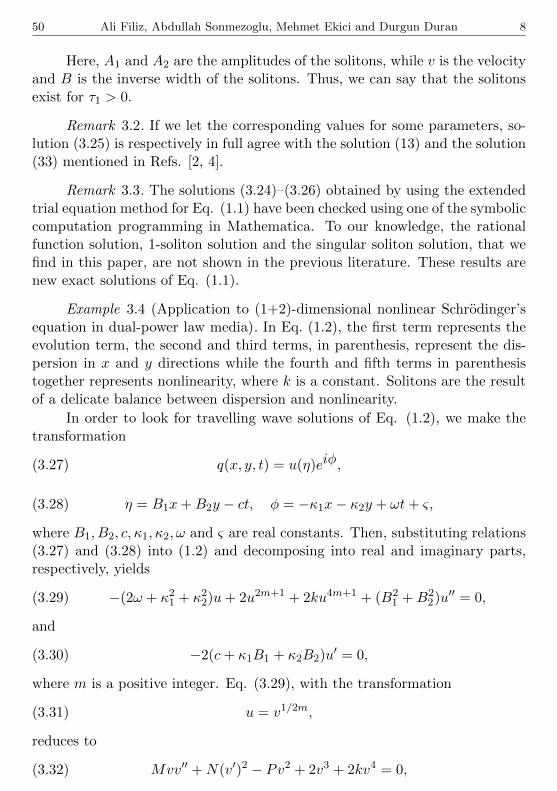
50 Ali Filiz, Abdullah Sonmezoglu, Mehmet Ekici and Durgun Duran 8

Here, A1 and A2 are the amplitudes of the solitons, while v is the velocityand B is the inverse width of the solitons. Thus, we can say that the solitonsexist for τ1 > 0.

Remark 3.2. If we let the corresponding values for some parameters, so-lution (3.25) is respectively in full agree with the solution (13) and the solution(33) mentioned in Refs. [2, 4].

Remark 3.3. The solutions (3.24)–(3.26) obtained by using the extendedtrial equation method for Eq. (1.1) have been checked using one of the symboliccomputation programming in Mathematica. To our knowledge, the rationalfunction solution, 1-soliton solution and the singular soliton solution, that wefind in this paper, are not shown in the previous literature. These results arenew exact solutions of Eq. (1.1).

Example 3.4 (Application to (1+2)-dimensional nonlinear Schrodinger’sequation in dual-power law media). In Eq. (1.2), the first term represents theevolution term, the second and third terms, in parenthesis, represent the dis-persion in x and y directions while the fourth and fifth terms in parenthesistogether represents nonlinearity, where k is a constant. Solitons are the resultof a delicate balance between dispersion and nonlinearity.

In order to look for travelling wave solutions of Eq. (1.2), we make thetransformation

(3.27) q(x, y, t) = u(η)eiφ,

(3.28) η = B1x+B2y − ct, φ = −κ1x− κ2y + ωt+ ς,

where B1, B2, c, κ1, κ2, ω and ς are real constants. Then, substituting relations(3.27) and (3.28) into (1.2) and decomposing into real and imaginary parts,respectively, yields

(3.29) −(2ω + κ21 + κ22)u+ 2u2m+1 + 2ku4m+1 + (B21 +B2

2)u′′ = 0,

and

(3.30) −2(c+ κ1B1 + κ2B2)u′ = 0,

where m is a positive integer. Eq. (3.29), with the transformation

(3.31) u = v1/2m,

reduces to

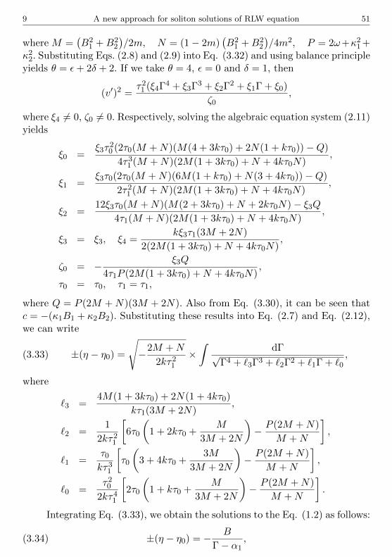
(3.32) Mvv′′ +N(v′)2 − Pv2 + 2v3 + 2kv4 = 0,

9 A new approach for soliton solutions of RLW equation 51

where M =(B2

1 +B22

)/2m, N = (1− 2m)

(B2

1 +B22

)/4m2, P = 2ω+κ21+

κ22. Substituting Eqs. (2.8) and (2.9) into Eq. (3.32) and using balance principleyields θ = ε+ 2δ + 2. If we take θ = 4, ε = 0 and δ = 1, then

(v′)2 =τ21 (ξ4Γ

4 + ξ3Γ3 + ξ2Γ

2 + ξ1Γ + ξ0)

ζ0,

where ξ4 6= 0, ζ0 6= 0. Respectively, solving the algebraic equation system (2.11)yields

ξ0 =ξ3τ

20 (2τ0(M +N)(M(4 + 3kτ0) + 2N(1 + kτ0))−Q)

4τ31 (M +N)(2M(1 + 3kτ0) +N + 4kτ0N),

ξ1 =ξ3τ0(2τ0(M +N)(6M(1 + kτ0) +N(3 + 4kτ0))−Q)

2τ21 (M +N)(2M(1 + 3kτ0) +N + 4kτ0N),

ξ2 =12ξ3τ0(M +N)(M(2 + 3kτ0) +N + 2kτ0N)− ξ3Q

4τ1(M +N)(2M(1 + 3kτ0) +N + 4kτ0N),

ξ3 = ξ3, ξ4 =kξ3τ1(3M + 2N)

2(2M(1 + 3kτ0) +N + 4kτ0N),

ζ0 = − ξ3Q

4τ1P (2M(1 + 3kτ0) +N + 4kτ0N),

τ0 = τ0, τ1 = τ1,

where Q = P (2M +N)(3M + 2N). Also from Eq. (3.30), it can be seen thatc = −(κ1B1 + κ2B2). Substituting these results into Eq. (2.7) and Eq. (2.12),we can write

(3.33) ±(η − η0) =

√−2M +N

2kτ21×∫

dΓ√Γ4 + `3Γ3 + `2Γ2 + `1Γ + `0

,

where

`3 =4M(1 + 3kτ0) + 2N(1 + 4kτ0)

kτ1(3M + 2N),

`2 =1

2kτ21

[6τ0

(1 + 2kτ0 +

M

3M + 2N

)− P (2M +N)

M +N

],

`1 =τ0kτ31

[τ0

(3 + 4kτ0 +

3M

3M + 2N

)− P (2M +N)

M +N

],

`0 =τ20

2kτ41

[2τ0

(1 + kτ0 +

M

3M + 2N

)− P (2M +N)

M +N

].

Integrating Eq. (3.33), we obtain the solutions to the Eq. (1.2) as follows:

(3.34) ±(η − η0) = − B

Γ− α1,

52 Ali Filiz, Abdullah Sonmezoglu, Mehmet Ekici and Durgun Duran 10

(3.35) ±(η − η0) =2B

α1 − α2

√Γ− α2

Γ− α1, α2 > α1,

(3.36) ±(η − η0) =B

α1 − α2ln

∣∣∣∣Γ− α1

Γ− α2

∣∣∣∣ ,±(η − η0) =

B√(α1 − α2)(α1 − α3)

× ln

∣∣∣∣∣√

(Γ− α2)(α1 − α3)−√

(Γ− α3)(α1 − α2)√(Γ− α2)(α1 − α3) +

√(Γ− α3)(α1 − α2)

∣∣∣∣∣ ,(3.37)

α1 > α2 > α3,

(3.38) ±(η − η0) = 2

√B

(α1 − α3)(α2 − α4)F (ϕ, l), α1 > α2 > α3 > α4,

where

B =

√−2M +N

2kτ21, F (ϕ, l) =

∫ ϕ

0

dψ√1− l2 sin2 ψ

,

and

ϕ = arcsin

√(Γ− α1)(α2 − α4)

(Γ− α2)(α1 − α4), l2 =

(α2 − α3)(α1 − α4)

(α1 − α3)(α2 − α4).

Also α1, α2, α3 and α4 are the roots of the polynomial equation

Γ4 +ξ3ξ4

Γ3 +ξ2ξ4

Γ2 +ξ1ξ4

Γ +ξ0ξ4

= 0.

Substituting the solutions (3.34)–(3.37) into (2.6) and (3.31), and settingv = −(κ1B1 + κ2B2), we obtain

(3.39) q(x, y, t) =

τ0 + τ1α1 ∓

τ1B

B1x+B2y − vt− η0

12m

eiφ,

(3.40)

q(x, y, t) =

τ0 + τ1α1 +

4B2(α2 − α1)τ1

4B2 − [(α1 − α2) (B1x+B2y − vt− η0)]2

12m

eiφ,

(3.41)

q(x, y, t) =

τ0 + τ1α2 +(α2 − α1)τ1

exp

(α1 − α2

B(B1x+B2y − vt− η0)

)− 1

1

2m

eiφ,

11 A new approach for soliton solutions of RLW equation 53

(3.42)

q(x, y, t) =

τ0 + τ1α1 +(α1 − α2)τ1

exp

(α1 − α2

B(B1x+B2y − vt− η0)

)− 1

1

2m

eiφ,

(3.43)

q(x, y, t) =

τ0 + τ1α1 −2A22τ1

A11 + (α3 − α2) cosh

(√A22

B

(A33

))

12m

eiφ,

where A11 = 2α1−α2−α3, A22 = (α1−α2)(α1−α3) and A33 = B1x+B2y−vt.If we take τ0 = −τ1α1 and η0 = 0, then the solutions (3.39)–(3.43) can reduceto rational function solutions

(3.44) q(x, y, t) =

(∓ τ1B

B1x+B2y − vt

) 12m

ei(−κ1x− κ2y + ωt+ ς),

(3.45)

q(x, y, t)=

4B2(α2 − α1)τ1

4B2 − [(α1 − α2) (B1x+B2y − vt)]2

12m

ei(−κ1x− κ2y + ωt+ ς),

traveling wave solutions

(3.46)

q(x, y, t) =

(α2 − α1)τ1

2

1∓ coth

[α1 − α2

2B(B1x+B2y − vt)

] 12m

ei(−κ1x− κ2y + ωt+ ς),

and soliton solution (see Figure 3)(3.47)

q(x, y, t) =A3(

D + cosh[K(B1x+B2y − vt)

]) 12m

ei(−κ1x− κ2y + ωt+ ς),

where

A3=

(2(α1−α2)(α1−α3)τ1

α3−α2

) 12m

, D=2α1−α2−α3

α3−α2, K=

√(α1−α2)(α1−α3)

B.

Here in (3.47), A3 is the amplitude of the soliton, B1 is the inverse widthof soliton in the x−direction and B2 is the inverse width of soliton in the

54 Ali Filiz, Abdullah Sonmezoglu, Mehmet Ekici and Durgun Duran 12

y−direction and v is the velocity of the soliton. Also κ1 and κ2 represents thesoliton frequency in the x and y directions respectively, while ω represents thesolitary wave number and finally ς is the phase constant of the soliton. Thus,we can say that the solitons exist for τ1 < 0.

Fig. 3 – Profile of the solution (3.47) corresponding to the values

A23 = 8/3, B = 1, B1 = 1, B2 = 6, D = 5/3, K = 2, m = 1 while vt = 1.

Remark 3.5. If we let the corresponding values for some parameters, so-lution (3.47) is in full agree with the solution (16) mentioned in Ref. [3].

Remark 3.6. The solutions (3.44)–(3.47) obtained by using the extendedtrial equation method for Eq. (1.2) have been checked again by Mathematica.To our knowledge, the rational function solutions and the soliton solution ob-tained using the method described in this paper are not shown in the previousliterature. These are new wave solutions of Eq. (1.2).

4. CONCLUSION

In this brief review we introduced the RLW equation and the NLSE, anddiscussed some of their remarkable features. The 1-soliton solution separatesbetween periodic wave solutions. Basic features of the 1-soliton solution, thesingular soliton solution and the soliton solution were discussed. We proposeda new trial equation method as an alternative approach to obtain the analyticsolutions of nonlinear partial differential equations with generalized evolutionin mathematical physics. In the quadratic choice of the trial equation, thefunction N of (2.5) is a polynomial where only even powers of (u′)2 appear.

13 A new approach for soliton solutions of RLW equation 55

Consequently, the solutions of the extended trial equation method includes thesolutions obtained by the standard approach [12]. One obtains only the exacttraveling wave solutions by the standart method. On the other hand, with theextended trial equation method, we can get not only the exact traveling wavesolutions, but the soliton solutions, the singular soliton solutions, the rationalfunction solutions and the elliptic function solutions, as well. We use theextended trial equation method aided with symbolic computation to constructthe soliton solutions, the elliptic function and rational function solutions forthe RLW equation and (1+2)-dimensional NLSE in dual-power law media. Theelliptic function solutions obtained by the present approach are more generalthan those obtained earlier.

Acknowledgments. We would like to thank the referees for their valuable suggestionswhich improved the manuscript.

REFERENCES

[1] M.A. Abdou, The extended tanh method and its applications for solving nonlinear phys-ical models. Appl. Math. Comput. 190 (2007), 988–996.

[2] A. Biswas, Solitary waves for power-law regularized long-wave equation and R(m,n) equa-tion. Nonlinear Dyn. 59 (2010), 423–426.

[3] A. Biswas, 1-soliton solution of (1+2)-dimensional nonlinear Schrodinger’s equation indual-power law media. Phys. Lett. A 372 (2008), 5941–5943.

[4] Y. Gurefe, E. Misirli, A. Sonmezoglu and M. Ekici, Extended trial equation method togeneralized nonlinear partial differential equations. Appl. Math. Comput. 219 (2013),5253–5260.

[5] Y. Gurefe, A. Sonmezoglu and E. Misirli, Application of an irrational trial equationmethod to high-dimensional nonlinear evolution equations. J. Adv. Math. Stud. 5(1)(2012), 41–47.

[6] Y. Gurefe and E. Misirli, Exp-function method for solving nonlinear evolution equationswith higher order nonlinearity. Comput. Math. Appl. 61 (2011), 2025–2030.

[7] Y. Gurefe and E. Misirli, New variable separation solutions of two-dimensional Burgerssystem. Appl. Math. Comput. 217 (2011), 9189–9197.

[8] Y. Gurefe, A. Sonmezoglu and E. Misirli, Application of the trial equation method forsolving some nonlinear evolution equations arising in mathematical physics. Pramana-J.Phys. 77(6) (2011), 1023–1029.

[9] R. Hirota, Exact solutions of the Korteweg-de-Vries equation for multiple collisions ofsolitons. Phys. Lett. A 27 (1971), 1192–1194.

[10] C.S. Liu, Applications of complete discrimination system for polynomial for classifica-tions of traveling wave solutions to nonlinear differential equations. Comput. Phys.Commun. 181 (2010), 317–324.

[11] C.S. Liu, A new trial equation method and its applications. Commun. Theor. Phys. 45(2006), 395–397.

[12] C.S. Liu, Trial equation method for nonlinear evolution equations with rank inhomoge-neous: mathematical discussions and applications. Commun. Theor. Phys. 45 (2006),219–223.

[13] C.S. Liu, Trial equation method and its applications to nonlinear evolution equations.Acta. Phys. Sin. 54 (2005), 2505–2509.

56 Ali Filiz, Abdullah Sonmezoglu, Mehmet Ekici and Durgun Duran 14

[14] C.S. Liu, Using trial equation method to solve the exact solutions for two kinds of KdVequations with variable coefficients. Acta. Phys. Sin. 54 (2005), 4506–4510.

[15] W. Malfliet and W. Hereman, The tanh method: exact solutions of nonlinear evolutionand wave equations. Phys. Scr. 54 (1996), 563–568.

[16] Y. Pandir, Y. Gurefe, U. Kadak and E. Misirli, Classification of exact solutions for somenonlinear partial differential equations with generalized evolution. Abstr. Appl. Anal.2012 (2012), Article ID 478531, 16 pp.

[17] H.X. Wu and J.H. He, Exp-function method and its application to nonlinear equations.Chaos Solitons Fractals 30 (2006), 700–708.

Received 9 December 2012 “Adnan Menderes” University,Faculty of Science and Arts,Department of Mathematics,

09010 Aydin, Turkeyafiliz@adu.edu.tr

Bozok University,Faculty of Science and Arts,Department of Mathematics,

66100 Yozgat, Turkeyabdullah.sonmezoglu@bozok.edu.tr

Bozok University,Faculty of Science and Arts,Department of Mathematics,

66100 Yozgat, Turkeymehmet.ekici@bozok.edu.tr

Bozok University,Faculty of Science and Arts,

Department of Physics,66100 Yozgat, Turkey

durgun.duran@bozok.edu.tr