A NEUROMOTOR MODEL OF HANDWRITING GENERATION: HIGHLIGHTING...
123
A NEUROMOTOR MODEL OF HANDWRITING GENERATION: HIGHLIGHTING THE ROLE OF BASAL GANGLIA A THESIS submitted by G.GANGADHAR For the award of the degree Of MASTER OF SCIENCE DEPARTMENT OF ELECTRICAL ENGINEERING INDIAN INSTITUTE OF TECHNOLOGY - MADRAS APRIL 2006
Transcript of A NEUROMOTOR MODEL OF HANDWRITING GENERATION: HIGHLIGHTING...
A NEUROMOTOR MODEL OF HANDWRITING GENERATION:
HIGHLIGHTING THE ROLE OF BASAL GANGLIA
A THESIS
submitted by
G.GANGADHAR
For the award of the degree
Of
MASTER OF SCIENCE
DEPARTMENT OF ELECTRICAL ENGINEERING
INDIAN INSTITUTE OF TECHNOLOGY - MADRAS APRIL 2006
THESIS CERTIFICATE
This is to certify that the thesis entitled A NEUROMOTOR MODEL OF
HANDWRITING GENERATION: Highlighting the Role of Basal Ganglia submitted
by Garipelli Gangadhar to Indian Institute of Technology, Madras for the award of
Master of Science by Research is a bonafide record of research work carried out by him
under my supervision. The contents in this thesis, in full or in parts, have not been
submitted to any other Institute of University for the award of any degree or diploma.
Madras 600036 Research Guide
Date:
ii
ACKNOWLEDGEMENTS
I express my sincere gratitude to my research guide Dr. V. Srinivasa Chakravarthy, for
his constant support, guidance and encouragement throughout the project and without
whose help the completion of this thesis would have been difficult. His enthusiasm for the
subject has been a great of source of inspiration for me.
I thank My GTC Members, Dr. Hema A. Murthy and Dr. A. N. Rajagopalan for their
valuable reviews.
I thank Dr. Bapiraju, University of Hyderabad for healthy criticism and stimulating
conversation in the middle of the thesis work.
I thank Dr. Rohith Manchanda, IIT Bombay for his encouragement in doing research in
computational neuroscience.
I am greatly indebted to Dr. Suresh Devasahayam, CMC Vellore, for his valuable
suggestions and reviews of my work.
I thank Dr. K. Sridharan for his kind help and valuable suggestions during my research
work.
I acknowledge Karthikeyan and Arun Kumar for their continuous discussions and
encouragement. I thank P.S. Prashanth, Dinesh, Gunjan, Anchal and J. Srinivas for their
assistance during the research work. I thank K. Umender, Rajiv Ranjan Sahay and N.
Rajeev Lochan who made my stay at IIT-M memorable. My gratitude to my lab members,
particularly Krishnan and Ranjan Kumar Pradhan for their valuable assistance during
the work.
I am grateful to my parents, brother and my sister for their support and encouragement.
Gangadhar Garipelli
iii
ABSTRACT
Keywords: Handwriting; Handwriting generation; Motor preparation; Basal ganglia;
Reinforcement learning; Parkinson’s disease; Computational neuroscience; Motor control;
Oscillatory neural networks.
Handwriting (HW), unlike reaching or walking, is a high-level motor activity, engaging
large parts of cortical and sub-cortical regions that include supplementary motor area
(SMA), premotor area (PM), primary motor area (M1), basal ganglia (BG), cerebellum,
spinal cord etc. Since each of these regions contributes to HW output in its own unique
fashion, pathology of any of these regions is manifest as characteristic features in HW. For
example, in Parkinson’s disease, a disorder of BG, HW is marked by diminutive letter size
or micrographia. Recognition of rich diagnostic value of HW had prompted a systematic
study of HW and the extensive neuromotor organization that generates it. Computational
modeling offers an integrative framework in which results of such studies – which come
from several domains, like behavioral, imaging, etc – are brought together and given a
concrete shape. An integrative computational model of human motor system and BG is
proposed. Dopamine deficient conditions as in PD patients are simulated in the model to
reproduce PD-like handwriting features like micrographia, fluctuating velocities, jagged
contour etc.
The model primarily consists of a neuromotor model which is capable of learning and
generating strokes, and a timing model which coordinates events in the neuromotor model.
In the neuromotor model of handwritten stroke generation, stroke velocities are expressed
as a Fourier-style decomposition of oscillatory neural activities. The timing network, which
resembles the timing action of BG, controls the events in the neuromotor model. The model
gives a precise description of what is loosely termed as “motor preparation,” involving a
dynamic interaction between BG and SMA. The model is further extended for multiple
stroke production. The special emphasis given to BG in the models qualifies it as a
candidate model for Parkinsonian handwriting. It is shown that model “pathologies” can
capture several features of Parkinsonian handwriting like micrographia, irregular velocity
profiles etc.
iv
TABLE OF CONTENETS
Page
ACKNOWLEDGEMENTS……………………………………………………………...ii
ABSTRACT......................................................................................................................iii
LIST OF TABLES………………………………………………………………………vii
LIST OF FIGURES…………………………………………………………………….viii
ABBREVIATIONS ……………………………………………………………………xiv
CHAPTER 1 INTRODUCTION……………………………………………………….1
1.1 Handwriting as a Diagnostic Tool…………………………………………….1
1.2 Computational Models of Handwriting Generation…………………………..2
1.3 Parkinson’s Disease and Basal Ganglia……………………………………….4
1.4 Computational Neuroscience and Disease Models……………………………5
1.5 Model of Parkinsonian Handwriting…………………………………………..6
1.6 Organization of the Report…………………………………………………….7
CHAPER 2 AN OSCILLATORY NEUROMOTOR MODEL OF HANDWRITING
GENERATION ………………………………………………………….. 9
2.1 Handwriting and Handwriting Generation……………………………………..9
2.2 Models of Handwriting…………………………………………………………9
2.2.1 Hollerbach’s oscillation theory of handwriting………………………………. 10
2.2.2 Schomaker’s model.………………………………………………………….. 10
2.2.3 Kalveram’s model……………………………………………………………. 11
2.2.4 Plamondan’s model………………………………………………………….. 12
2.2.5 AVITEWRITE model…………………………………………………………12
2.3 Present Model…………………………………………………………………13
2.3.1 Single oscillator model………………………………………………………..14
2.3.2 Sublayer model: Ring of oscillators…………………………………………..15
2.3.3 Preparing the network state………………………………………………….. 16
v
Table of contents (continued) Page
2.3.4 The timing network…………………………………………………………….17
2.3.5 Network response……………………………………………………………....20
2.3.6 Training………………………………………………………………………...21
2.3.7 Summary……………………………………………………………………….25
CHAPTER 3 BASAL GANGLIA AS A SOURSE OF EXPLORATORY DRIVE:
A MODEL FOR REACHING…………………………………………………...26
3.1 Basal Ganglia…………………………………………………………………..26
3.1.1 Neuroanatomy of basal ganglia………………………………………………..26
3.1.2 Reward signaling in basal ganglia: How rewards lead to learning?...................29
3.2 Computational Models of Basal Ganglia………………………………………31
3.3 Present Model………………………………………………………………….38
3.3.1 Architecture of proposed model ………………………………………………38
3.3.2 Training phase: Exploration and consolidation ……………………………….46
3.3.3 Summary……………………………………………………………………….49
CHPTER 4 UNDERSTANDING PARKINSONIAN HANDWRITING THROUGH
A COMPUTATIONAL MODEL………………………………………..50
4.1 Introduction…………………………………………………………………….50
4.2 Parkinson’s Disease …………………………………………………………...51
4.3 Handwriting in Parkinson’s Disease and Need for a Computational Model…..54
4.4 Literature review of Models of Parkinson’s Disease………………………….55
4.5 Present Model.…………………………………………………………………57
4.6 Summery……………………………………………………………………….61
CHAPTER 5 RESULTS…………………………………………………………………62
5.1 Results of Chapter 2: A Model of Handwriting Generation…………………...62
5.1.1 Experiment 1: Are harmonics necessary? ……………………………………..62
vi
Table of contents (continued) Page
5.1.2 Experiment 2: Capacity of the network………………………………………..64
5.1.3 Experiment 3: No. of sublayers Vs No. of units per sublayer…………………65
5.1.4 Experiment 4: Studies on post preparatory delay ……………………………..65
5.1.5 Experiment 5: Origins of motor variability ………………………………….. 67
5.1.6 Experiment 6: Generating a stroke sequence …………………………………69
5.2 Results of Chapter 3: Basal Ganglia as a Source of Exploratory Drive:
A Model for Reaching ………………………………………………………. 76
5.3 Results of Chapter 4: A Model of Parkinonian Handwriting…………………77
5.3.1 Normal handwriting…………………………………………………………..78
5.3.2 Parkinsonian handwriting…………………………………………………….79
5.3.2 Batch results of Parkinsonian handwriting …………………………………..82
5.4 Summary……………………………………………………………………...84
CHAPTER 6 CONCLUSIONS……………………………………………………….. 85
REFERENCES…………………………………………………………………………..101
APPENDIX……………………………………………………………………………...107
vii
LIST OF TABLES
Table Title Page
1.1 Summary of Events in Handwriting Generation………………………….18
5.1 Mean of the Reconstruction error of strokes…………………………….. 65
viii
LIST OF FIGURES
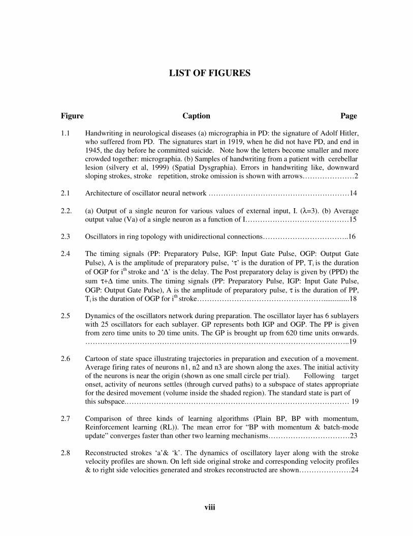
Figure Caption Page 1.1 Handwriting in neurological diseases (a) micrographia in PD: the signature of Adolf Hitler,
who suffered from PD. The signatures start in 1919, when he did not have PD, and end in
1945, the day before he committed suicide. Note how the letters become smaller and more
crowded together: micrographia. (b) Samples of handwriting from a patient with cerebellar
lesion (silvery et al, 1999) (Spatial Dysgraphia). Errors in handwriting like, downward
sloping strokes, stroke repetition, stroke omission is shown with arrows…………………2
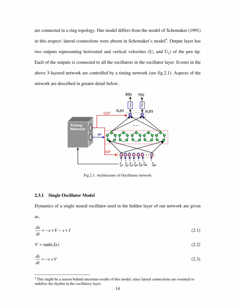
2.1 Architecture of oscillator neural network …………………………………………………14
2.2. (a) Output of a single neuron for various values of external input, I. (λ=3). (b) Average
output value (Va) of a single neuron as a function of I……………………………………15
2.3 Oscillators in ring topology with unidirectional connections……………………………..16
2.4 The timing signals (PP: Preparatory Pulse, IGP: Input Gate Pulse, OGP: Output Gate
Pulse), A is the amplitude of preparatory pulse, ‘τ’ is the duration of PP, Ti is the duration
of OGP for ith
stroke and ‘∆’ is the delay. The Post preparatory delay is given by (PPD) the
sum τ+∆ time units. The timing signals (PP: Preparatory Pulse, IGP: Input Gate Pulse,
OGP: Output Gate Pulse), A is the amplitude of preparatory pulse, τ is the duration of PP,
Ti is the duration of OGP for ith
stroke……………………………………………..............18
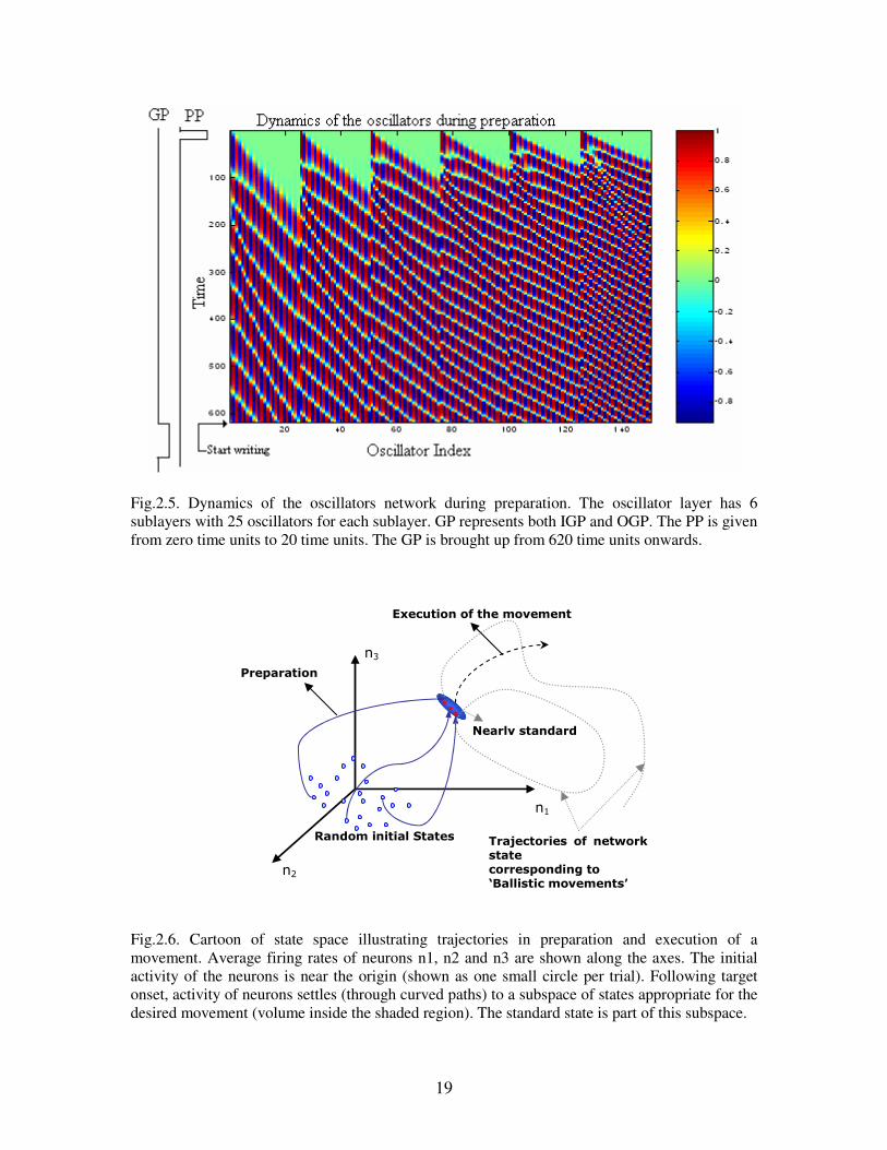
2.5 Dynamics of the oscillators network during preparation. The oscillator layer has 6 sublayers
with 25 oscillators for each sublayer. GP represents both IGP and OGP. The PP is given
from zero time units to 20 time units. The GP is brought up from 620 time units onwards.
……………………………………………………………………………………………..19
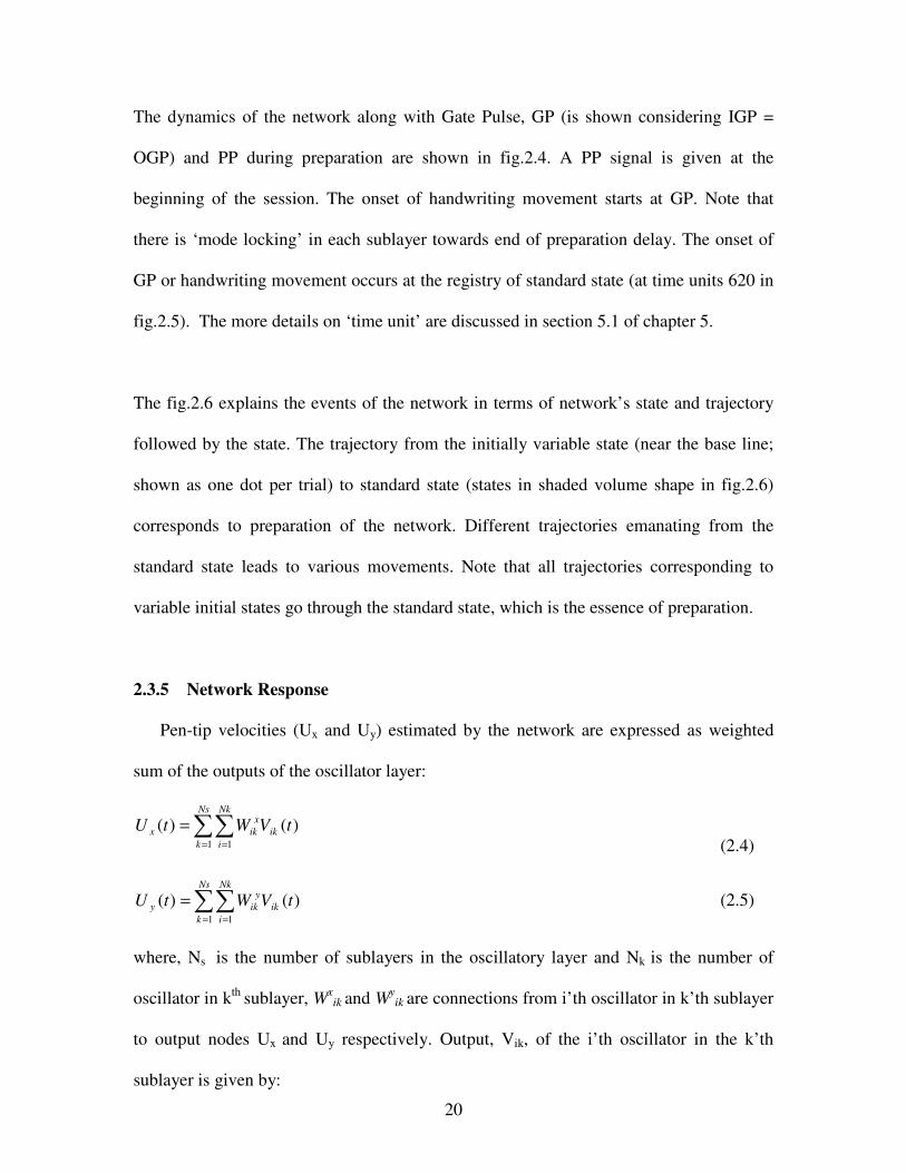
2.6 Cartoon of state space illustrating trajectories in preparation and execution of a movement.
Average firing rates of neurons n1, n2 and n3 are shown along the axes. The initial activity
of the neurons is near the origin (shown as one small circle per trial). Following target
onset, activity of neurons settles (through curved paths) to a subspace of states appropriate
for the desired movement (volume inside the shaded region). The standard state is part of
this subspace.……………………………………………………………………………… 19
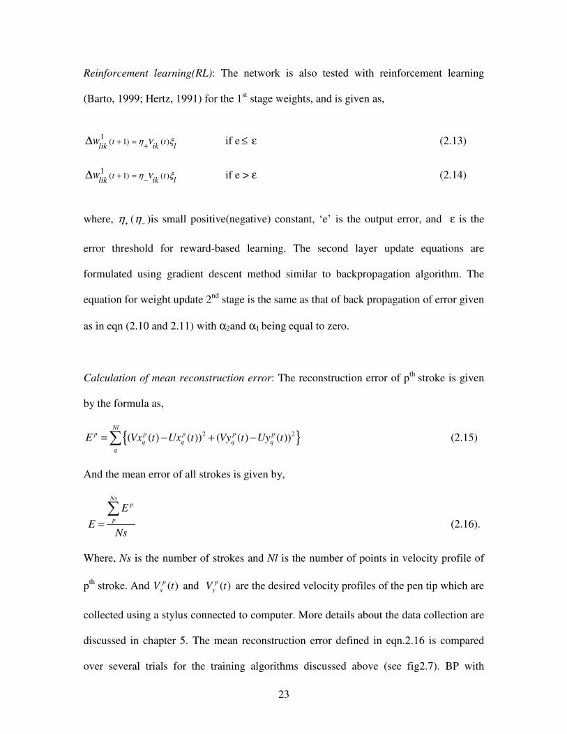
2.7 Comparison of three kinds of learning algorithms (Plain BP, BP with momentum,
Reinforcement learning (RL)). The mean error for “BP with momentum & batch-mode
update” converges faster than other two learning mechanisms……………………………23
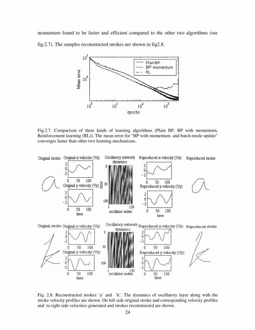
2.8 Reconstructed strokes ‘a’& ‘k’. The dynamics of oscillatory layer along with the stroke
velocity profiles are shown. On left side original stroke and corresponding velocity profiles
& to right side velocities generated and strokes reconstructed are shown…………………24
ix
3.1 Anatomical basis for motor functions in basal ganglia…………………………………….27
3.2 The direct and indirect pathways of basal ganglia……………………………………… 28
3.3 How rewards lead to learning? Steps involved in reward based learning. See text for the
explanation of these steps…………………………………………………………………. 30
3.4 Architecture of a model of basal ganglia…………………………………………………39
3.5. (a) STN – GPe neuron pair illustrating the excitatory & inhibitory connections, (b) Network
model of STN – GPe loop with lateral connections……………………………………….41
3.6 Dynamics of STN - GPe Loop: Three characteristic patterns of activity of the STN-GPe
layer – (a) chaotic, (b) traveling waves & (c) compact center. The three activity regimes
(from left to right) are obtained by progressively increasing ε from 0 to 2. Increasing ε
increases the percentage of positive lateral connections in STN. I n regime (c), “compact
center,” the array splits into a center and a surround, with neurons is either region forming a
synchronized cluster………………………………………………………………………..42
3.7 The convergence layer for STN-GPe Network………………………………………….....43
3.8 (a) A simple muscle model based on spring damper system (b) A single link configuration
with agonist and antagonist muscles ………………………………………………………44
3.9 (a) The 2-link arm model, (b) The workspace (shaded region; the origin corresponds to
elbow joint) of the 2-link arm with r1 = r2= r3= r4, h1 = h2, l1 = l2………………………….46
3.10 Microcircuit Illustrating Selection of Pathways Based on Dopamine Signal……………...48
4.1 Normal functional anatomy of basal ganglia………………………………………………52
4.2 Pathology of Parkinson’s disease …………………………………………………………53
4.3 Integrated neuromotor model of handwriting generation………………………………....60
4.4 Mapping the integrated model onto neuroanatomy……………………………………….60
5.1 Handwritten stroke set…………………………………………………………………….62
5.2 Mean of weights connecting each sublayer to second layer………………………………63
5.3. Strokes of the experiment 1 (a) Original Strokes, (b) Reproduced with harmonics,
(c) Reproduced without harmonics………………………………………………………..64
5.4 Reconstruction error of stroke vs. No of sublayers………………………………………. 64
5.5. Strokes corresponding to experiment on capacity of the network (a) Original strokes, (b)5
sublayers, (c) 3 sublayers and (d) 1 sublayer………………………………………………65
5.6. Reconstruction error and the corresponding reconstructed strokes for various PPDs.
(a) Strokes reconstructed with PPDs mentioned at the top of the strokes, (b) reconstruction
x
error as a function of PPD. (c) The deviation from the standard state with delay. Note
that the error is not a monotonic function of PPD. Error reaches small values at periodic
values of delay (PPD)………………………………………………………………………66
5.7 Demonstration of variability due to suboptimal gating pulse…………………………….. 68
5.8 Demonstration of variability due to random initial conditions…………………………….68
5.9 Demonstration of motor variability with unreliable input gating signals (a) variability due
to early drop in magnitude of IGP signal (b) variability due to late arrival of IGP signal.
Though the duration of IGP is reduced, the OGP is ON for the full duration between
“Standard State” and the “End of Stroke”………………………………………………….69
5.10. (a) The stroke sequence ‘elle’ generated with multiple preparations. The oscillatory
layer is prepared afresh for every stroke. (b) Deviation of network state from the standard
state at end of writing each stroke in sequence ‘elle’ (c) Deviation of Network State from
the standard state after preparation. In (b) along the x – axis the stroke indices Si are
shown(Si = 1,2,3 and 4 corresponding to ‘e’, ‘l’ , ‘l’ and ‘e’ respectively) and along y - axis
the distance is shown. The deviations before preparation are 4.75, 3.75, 3.75 and 4.75.
After preparation all the distances are less than 0.2 ……………………………………….70
5.11. Generation of stroke sequence ‘elle’ with single preparation and fixed full duration input
gate pulse (IGP). (a) The generated stroke sequence, (b) the distance of deviation from the
networks state at the end of each stroke to the standard state. (c) Illustration of events in the
production of stroke sequence ‘elle’ with preparatory and gating signals. The oscillator
network is prepared only at the arrival of first input stroke command. There is no
preparation between strokes. The strokes are executed in continuous fashion one after other
without any delay. The first two strokes seem to be legible, but the later ones are not. The
execution time is reduced at the cost of legibility of the stroke. The oscillatory layer state
does not return to the “standard state”. The distances of the states of oscillatory layer from
the “standard state” just before the stroke onset are 3.3, 4.9, 5.15, and 4.75
respectively.………………………………………………………………………………..72
5.12. Generation of stroke sequence ‘elle’ with single preparation and partial duration input gate
pulse (IGP). (a) The generated stroke sequence, (b) the distance of deviation from the
networks state at the end of each stroke to the standard state. (c) The events during the
generation of the stroke sequence ‘elle’. The oscillator network is prepared only before the
first stroke. There is no preparation between strokes. But the IGP for a given stroke is not
ON throughout the stroke execution period, T. For example, IGP of stroke 1 is turned OFF
at ‘c1’ and IGP of stroke 2 is turned ON only at ‘a2’. Though the strokes generated with
this method are more legible that that of previous method, the legibility of the stroke
generated is not appreciable. The distances of the oscillatory layer state from the “standard
state” in this case are 2.7, 2.9, 3.4, and 4.5 respectively.......................................................74
5.13. Generation of stroke sequence ‘elle’ with fixed partial duration input gate pulse (IGP), and
with phase-triggered gating mechanism. (a) The generated stroke sequence, (b) Illustration
of the events during the generation for the stroke sequence ‘elle’. The oscillator network is
prepared only before the first stroke. There is inter–stroke delay during which the timing
network monitors the dynamics of oscillatory layer network. Once the standard phase is
reached the timing network enables input and output lines turning ON IGP and OGP. OGP
is allowed to be ON during the entire duration of the stroke, Tf, but the IGP is turned OFF
xi
before that, allowing the oscillator layer a brief “free-running” period. Stroke obtained by
this method are of better quality than those obtained by the two methods discussed……...75
5.14 Training Error………………………………………………………………………………77
5.15. The trajectories of the hand model corresponding to eight points around a circle. (a)
Learning with strong reward, the model reaches the targets (b) Learning with weak reward,
the model wanders around a target making a futile attempt to reach ………………….......77
5.16 (a) The simulated handwriting with DA=50 and ε = 0.0 corresponding to normal control.
(b) The dotted trajectory corresponding to (a) illustrates the speed of writing (sparse dots
show fast movement whereas dense dots show the slow movement) …………………….78
5.17 Signals corresponding to normal handwriting. DA = 50 and ε = 0.0, the sub plots show
OGPx , OGPy , Ux , Uy and snap shots of the dynamics of STN grid (each small square
correspond to activity of a STN cell on the grid of 20 x 20 of which back correspond to ‘0’
whereas white correspond to ‘1’) respectively from top to bottom………………………..78
5.18 (a) The simulated handwriting with DA=25 and ε = 0.0.corresponding to PD. (b) The
dotted trajectory corresponding to (a) illustrates the speed of writing (sparse dots show fast
movement whereas dense dots show the slow movement)………………………………...80
5.19 Signals corresponding to PD handwriting with DA = 25 and ε = 0.0 corresponding to
micrographia and bradykinesia. The sub plots show OGPx , OGPy , Ux , Uy and snap shots of
the dynamics of STN grid(each small square correspond to activity of a STN cell on the
grid of 20 x 20 of which back correspond to ‘0’ where as white correspond to ‘1’)
respectively from top to bottom……………………………………………………………80
5.20 (a) The simulated handwriting with DA=50 and ε = 0.6. (b) The dotted trajectory
corresponding to (a) illustrates the speed of writing (sparse dots show fast movement
whereas dense dots show the slow movement)……………………………………………81
5.21 Signals corresponding to PD handwriting with DA = 50 and ε = 0.6 corresponding to
jagged/ wavy handwriting. The sub plots show OGPx , OGPy , Ux , Uy and snap shots of the
dynamics of STN grid respectively from top to bottom…………………………………...81
5.22 (a) The simulated handwriting with DA=25 and ε = 0.6.corresponding to PD. (b) The
dotted trajectory corresponding to (a) illustrates the speed of writing (sparse dots show fast
movement whereas dense dots show the slow movement)………………………………...82
5.23 PD handwriting with DA = 25 and ε = 0.6 corresponding both micrographia and jagged
handwriting. The sub plots show OGPx , OGPy , Ux , Uy and snap shots of the dynamics of
STN grid(each small square correspond to activity of a STN cell on the grid of 20 x 20 of
which back correspond to ‘0’ where as white correspond to ‘1’) respectively from top to
bottom …………………………………………………………………………………….82
5.24 The simulated handwriting corresponding to various levels of dopamine (DA) andε. DA
decreases as along x – axis from right to left. The parameter ε increases along y axis from
xii
top to bottom. Aspects of normal handwriting and Parkinsonion handwriting (like
micrographia, jagged contour etc) are captured by the model outputs. …………………...83
6.1 Overview of Motor System ………………………………………………………………..87
6.2 Pin-Ball Game model of Motor System and Movement Generation ………………….......88
A.1 The state variable, ‘x’ Vs the odd function, ‘F(x)’………………………………………..102
xiii
ABBREVIATIONS
ARP Associative Reward Penalty
AVITEWRITE Vector Integration to Endpoint WRITE
BG Basal Ganglia
BP momentum Backpropagation algorithm with momentum
BP Bereitschafts Potential
GP Gate Pulse
GPe Globus Pallidus external
GPi Globus Pallidus internal
HW Handwriting
ICSS Intra Cranial Self Stimulation
IGP Input Gate Pulse
M1 Primary Motor area
OGP Output Gate Pulse
PD Parkinson’s Disease
Plain BP Plain Backpropagation algorithm
PM Pre Motor Area
PMd dorsolateral Premotor Area
PP Preparatory Pulse
PPD Post Preparatory Delay
RL Reinforcement Learning
SMA Supplementary Motor Area
SNc Substantia Nigra pars compcta
SNr Substantia Nigra pars reticula
SOM Self Organizing Map
STN Subthalamic nucleus
STR Striatum
TD Temporal Difference
VTA Ventral Tegmental Area
CHAPTER 1
INTRODUCTION
1.1 HANDWRITING AS A DIAGNOSTIC TOOL
Handwriting is a learned, highly practiced human motor skill that involves the control
and coordination of complex movement sequences. In the past decade (Cobbah, M.C.
and Fairhrust, 2000; Kuenstler et al, 1999; van Gemmert et al, 1999), handwriting has
been gaining attention as a source of diagnostic information, which carries precise
signatures of a variety of neurological disorders including Parkinson’s disease (van
Gemmert et al; 1999; Teulings et al, 2002), Schizophrenia (Gallucci et al, 1997),
Obsessive Compulsive Disorder (Marvogiorgou et al, 2001) etc. Since handwriting,
unlike reaching or walking, is a high-level motor activity, it engages large parts of
cortical and subcortical regions that include Supplementary motor area (SMA), Premotor
area (PM), Primary motor area (M1), Basal ganglia (BG), Cerebellum, Spinal cord etc.
Since each of these regions contributes to handwriting output in its own unique fashion,
pathology of any of these regions is manifest as characteristic features in handwriting.
For example, in Parkinson’s disease, a disorder of BG, handwriting is marked by
diminutive letter size or micrographia (fig.1.a). Similarly handwriting in patients with
cerebellar damage is often characterized by omissions and unnecessary repetition of
strokes (fig.1.b). Recognition of rich diagnostic value of handwriting had prompted a
systematic study of handwriting and the extensive neuromotor organization that generates
it. Computational modeling offers an integrative framework in which results of such
studies – which come from several domains, like behavioral, imaging, etc – are brought
together and given a concrete shape. Several computational models of handwriting
2
production have been developed to investigate the complex interaction among these
structures.
(a) (b)
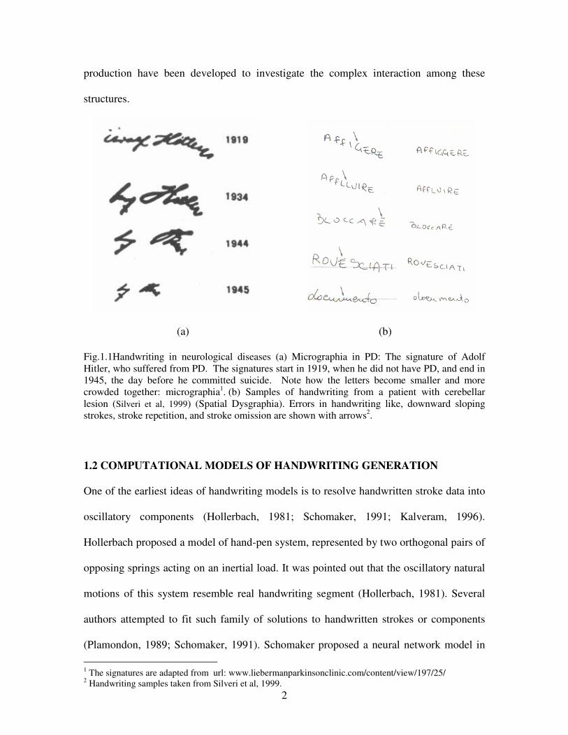
Fig.1.1Handwriting in neurological diseases (a) Micrographia in PD: The signature of Adolf
Hitler, who suffered from PD. The signatures start in 1919, when he did not have PD, and end in
1945, the day before he committed suicide. Note how the letters become smaller and more
crowded together: micrographia1. (b) Samples of handwriting from a patient with cerebellar
lesion (Silveri et al, 1999) (Spatial Dysgraphia). Errors in handwriting like, downward sloping
strokes, stroke repetition, and stroke omission are shown with arrows2.
1.2 COMPUTATIONAL MODELS OF HANDWRITING GENERATION
One of the earliest ideas of handwriting models is to resolve handwritten stroke data into
oscillatory components (Hollerbach, 1981; Schomaker, 1991; Kalveram, 1996).
Hollerbach proposed a model of hand-pen system, represented by two orthogonal pairs of
opposing springs acting on an inertial load. It was pointed out that the oscillatory natural
motions of this system resemble real handwriting segment (Hollerbach, 1981). Several
authors attempted to fit such family of solutions to handwritten strokes or components
(Plamondon, 1989; Schomaker, 1991). Schomaker proposed a neural network model in
1 The signatures are adapted from url: www.liebermanparkinsonclinic.com/content/view/197/25/
2 Handwriting samples taken from Silveri et al, 1999.
3
which a network of oscillators outputs horizontal and vertical pen motion (Schomaker,
1991). Network training, performed using a variation of delta-rule, led to uncertain
results. More recently Kalveram proposed a model in which stroke data is resolved to its
Fourier components (Kalveram, 1996). An oscillatory neural model of handwriting, for it
to be biologically viable, has to address certain fundamental issues. The first key issue,
one of preparing the initial state of the oscillatory network, does not seem to have
received adequate attention (Schomaker, 1991; Kalveram, 1996). Essentially there is a
need for auxiliary mechanisms that 1) initiate/prepare (a rhythm in the oscillatory
network’s state), 2) that align (that rhythm with respect to the time of onset of the stroke),
and 3) terminate (the rhythm at the appropriate time).
The neuromotor model of handwritten stroke generation presented in this thesis addresses
the issues discussed above. In line with oscillatory theories of handwriting, the present
model consists of a network of neural oscillators, which learns to resolve a handwritten
stroke into its oscillatory components. A key component of the model is a timing network
which coordinates the events occurring in various parts of the network like stroke
initiation, output gating etc. The action of this timing network has close resemblances to
that of BG in human motor function. Specifically, its role in preparing the state of
appropriate motor cortical areas prior to initiation of motor act is highlighted by the
model. The special emphasis given to BG in our models qualifies it as a candidate model
for Parkinsonian handwriting. It will be shown that model “pathologies” can capture
several features of Parkinsonian handwriting like micrographia, irregular velocity profiles
etc.
4
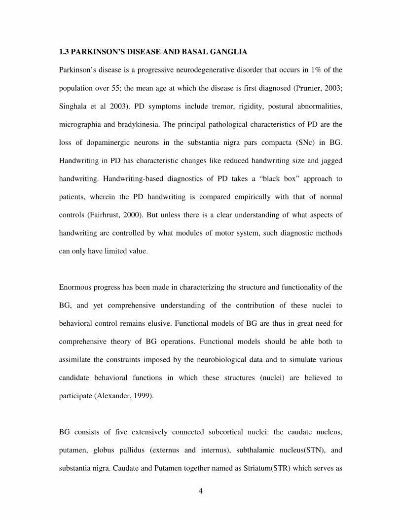
1.3 PARKINSON’S DISEASE AND BASAL GANGLIA
Parkinson’s disease is a progressive neurodegenerative disorder that occurs in 1% of the
population over 55; the mean age at which the disease is first diagnosed (Prunier, 2003;
Singhala et al 2003). PD symptoms include tremor, rigidity, postural abnormalities,
micrographia and bradykinesia. The principal pathological characteristics of PD are the
loss of dopaminergic neurons in the substantia nigra pars compacta (SNc) in BG.
Handwriting in PD has characteristic changes like reduced handwriting size and jagged
handwriting. Handwriting-based diagnostics of PD takes a “black box” approach to
patients, wherein the PD handwriting is compared empirically with that of normal
controls (Fairhrust, 2000). But unless there is a clear understanding of what aspects of
handwriting are controlled by what modules of motor system, such diagnostic methods
can only have limited value.
Enormous progress has been made in characterizing the structure and functionality of the
BG, and yet comprehensive understanding of the contribution of these nuclei to
behavioral control remains elusive. Functional models of BG are thus in great need for
comprehensive theory of BG operations. Functional models should be able both to
assimilate the constraints imposed by the neurobiological data and to simulate various
candidate behavioral functions in which these structures (nuclei) are believed to
participate (Alexander, 1999).
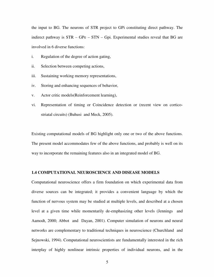
BG consists of five extensively connected subcortical nuclei: the caudate nucleus,
putamen, globus pallidus (externus and internus), subthalamic nucleus(STN), and
substantia nigra. Caudate and Putamen together named as Striatum(STR) which serves as
5
the input to BG. The neurons of STR project to GPi constituting direct pathway. The
indirect pathway is STR – GPe – STN – Gpi. Experimental studies reveal that BG are
involved in 6 diverse functions:
i. Regulation of the degree of action gating,
ii. Selection between competing actions,
iii. Sustaining working memory representations,
iv. Storing and enhancing sequences of behavior,
v. Actor critic models(Reinforcement learning),
vi. Representation of timing or Coincidence detection or (recent view on cortico-
striatal circuits) (Buhusi and Meck, 2005).
Existing computational models of BG highlight only one or two of the above functions.
The present model accommodates few of the above functions, and probably is well on its
way to incorporate the remaining features also in an integrated model of BG.
1.4 COMPUTATIONAL NEUROSCIENCE AND DISEASE MODELS
Computational neuroscience offers a firm foundation on which experimental data from
diverse sources can be integrated; it provides a convenient language by which the
function of nervous system may be studied at multiple levels, and described at a chosen
level at a given time while momentarily de-emphasizing other levels (Jennings and
Aamodt, 2000; Abbot and Dayan, 2001). Computer simulation of neurons and neural
networks are complementary to traditional techniques in neuroscience (Churchland and
Sejnowski, 1994). Computational neuroscientists are fundamentally interested in the rich
interplay of highly nonlinear intrinsic properties of individual neurons, and in the
6
coupling properties between cells that determine the dynamical activity of neuronal
networks (Abbot and Dayan, 2001). These models describe neural organization and
dynamics at many levels of abstraction of the physical processes and anatomical units, at
a range of spatial and temporal scales – short-term to long-term changes (Jennings and
Aamodt, 2000).
Computational modeling of neurological disease represents a new research paradigm,
competing with traditional methods such as clinical studies and animal models (Reggia,
et al 1996). Computational models for neurological diseases like, Epilepsy (Silva and
Pijn, 1995), Alzheimer’s disease (Ruppin et al, 1996), Parkinson’s disease (Vidal et al,
1996; Terman et al, 2002; Teulings et al, 2003), Schizophrenia(Horn and Ruppin, 1995;
Grossberg, 1999), Autism(Bjorne, 2005; Grossberg, 2006), Dyslexia (Harm and
Seidenberg 1999), etc3 are developed to get insight into these diseases. “Pathologies” are
simulated with virtual neural models to study various brain and cognitive disorders. The
goals of such research is to construct computational models that can explain how specific
neuroanatomical and pathological changes can result in various clinical manifestations,
and to investigate the functional organization of symptoms that result from specific brain
pathologies(Reggia et al, 1996).
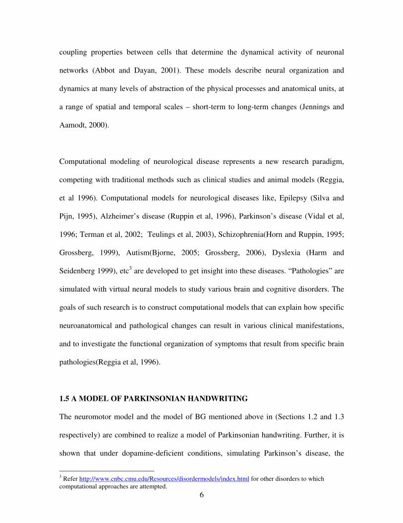
1.5 A MODEL OF PARKINSONIAN HANDWRITING
The neuromotor model and the model of BG mentioned above in (Sections 1.2 and 1.3
respectively) are combined to realize a model of Parkinsonian handwriting. Further, it is
shown that under dopamine-deficient conditions, simulating Parkinson’s disease, the
3 Refer http://www.cnbc.cmu.edu/Resources/disordermodels/index.html for other disorders to which
computational approaches are attempted.
7
model produces PD-like handwriting with micrographia, irregular velocity profile etc.
With the help of the present model it is possible to link signaling inside BG (e.g.,
dopamine signal, activity of STN-GPe etc.) to observable behavior, namely, handwriting.
The model is a “systems level,” neural network model of BG consisting of abstract
“neurons.” However, even this simple model provides tremendous insight into the nature
of BG, complete understanding of which eludes us to this day. For example the proposed
model suggests that complex activity of STN-GPe loop is essential for reinforcement
learning. Loss of this complexity is manifest as PD handwriting symptoms according to
the model. More detailed extensions of the present model might find applications in
several aspects of PD treatment: 1) in drug dosage determination, 2) in designing of
Deep Brain Stimulation protocols etc.
1.6 ORGANIZATION OF THE REPORT
The rest of the report is organized as follows: In chapter 2, a neuromotor model of
handwriting generation in which stroke velocities are expressed as a Fourier – style
decomposition of oscillatory neural activities is presented along with a review of the
existing handwriting models in the literature. Issues involved in the preparation of
oscillator network which are neglected the literature, were discussed and a solution is
attempted. Difficulties in multiple stroke generation were discussed and a solution is
proposed. Studies on preparatory delay, origins of motor variability and isochrony were
discussed. A possible mapping of the model on to neuroanatomy is attempted.
In Chapter 3, a model of reaching, involving BG is presented along with the literature
reviews of existing models of BG. A possible functional role of direct pathway and
indirect pathway were suggested.
8
Chapter 4 reviews PD models of handwriting. The proposed combined model of
neuromotor model of handwriting generation and BG model is presented along with
review of existing models of PD handwriting.
In Chapter 5 the results of neuromotor model of handwriting generation, model of
reaching involving BG and a model of PD handwriting were discussed. Finally the report
concludes with discussion of findings in the present work in Chapter 6.
9
CHAPTER 2
AN OSCILLATORY NEUROMOTOR MODEL OF
HANDWRITING GENERATION
To the theoretical question, can you design a machine to do whatever a brain can do?
The answer is this: If you will specify in a finite and unambiguous way what you think a brain
does ... then we can design a machine to do it...
But can you say what you think brain do?
– W. S .McCulloch
2.1 HANDWRITING AND HANDWRITING GENERATION
Handwriting (HW) is a learned, highly practiced human motor skill that involves the
control and coordination of several subsystems in our motor system. The production of
handwriting requires a hierarchically organized flow of information through various
transformations (Ellis 1998; Teulings et al 1986). The writer starts with the intention to
write a message (semantic level), which is transformed into words (lexical and syntactical
level). When the individual letters (graphemes) are known, the writer selects specific
letter shape variants (allographs). The selection is done with respect to the formal
allograph selection syntax, according to individual preference or just random choice
(Schomaker, 1991). Below this level, the allographs are transformed into movement
patterns, which is the object of focus of the present work.
2.2 MODELS OF HANDWRITING
Two general methodologies of handwriting modeling become apparent from the
literature. The first one, dubbed the “bottom-up” approach, refers to computational
models which attempt to empirically reproduce features of human writing such as
velocity and acceleration profiles etc; they do not claim any fidelity to neuromotor
processes underlying handwriting processes (Plamondon, 1989; Grossberg and Paine,
10
2000; Hollerbach, 1981; Kalveram, 1996). The second methodology of handwriting
modeling focuses on psychologically descriptive models (van Galen and Weber 1991,
Grossberg and Paine 2000). These “top-down” models usually summarize many issues
such as, motor learning, movement memory, planning and sequencing, coarticulatory and
task complexity of strokes, etc.
2.2.1 Hollerbach’s Oscillation Theory of Handwriting
An important class of handwriting models is centered on the philosophy that stroke data
can be resolved into certain oscillatory components by Fourier-style decomposition. The
approach was pioneered by Hollerbach (1981) who proposed an insightful model of
handwriting generation where the hand-pen system is represented by two orthogonal
pairs of opposing springs acting on an inertial load. It was pointed out that the oscillatory
natural motions of this system resemble real handwriting segments. Anatomical
justification of such a simple system has also been explored (Hollerbach, 1981).
2.2.2 Schomaker’s Model
Schomaker (1991) proposed a neural network model in which a network of oscillators
outputs horizontal and vertical pen motion. Network training, performed using a variation
of delta-rule, led to uncertain results: performance depended critically on network
parameters. In spite of the shortcomings of the performance of the model, Schomaker’s
work clearly elucidates certain issues related to any possible handwriting model.
Accordingly, the handwriting process – and hence its model – must have four basic
events or phases both in chaining and shaping of handwriting:
11
1. System configuration: This stage is known as motor programming, coordinative
structure gearing, preparation, planning, schema build-up etc.
2. Start of pattern: After configuring the system for the task at hand, there must be a
signal releasing the pattern.
3. Execution of pattern: The duration of this phase and actions that are performed
depend on pieces of information such as the amount of time that has passed, the
distance from a spatial target position or force target value, or even the number of
motor segments produced.
4. End of pattern: this stage deals with the termination of the movement.
Though the network includes important episodes during handwriting execution,
the network training, performed using a variation of delta-rule, led to uncertain results.
2.2.3 Kalveram’s Model
More recently Kalveram (1996) proposed a model in which stroke data is resolved into its
Fourier components. This simple mathematical operation is described using the metaphor
of ‘central target pattern generator’. The model in our view has several drawbacks. Since
a handwritten stroke – for that matter any real motor sequence – lives for a finite
duration, the dynamics of a system that produces it must be appropriately initiated and
terminated. Fourier decomposition assumes a set of oscillators with precise initialization
and phase-relationships. A network that performs such decomposition, and produces a
stroke by re-synthesis, has to be appropriately prepared. Accurate preparation of the
initial state may be crucial for successful stroke generation. Further, in a large network of
oscillators this preparation of the initial state can be a challenge in itself, in addition to
12
accurate stroke learning/acquisition and production. Another drawback is that in
(Kalveram, 1996) a separate network has to be trained for every stroke.
2.2.4 Plamondon’s Model
Plamondon and Guefali (1998) presented a bottom-up model using “delay-lognormal
synergies”. The name refers to author’s definition of the velocity of a muscle synergy as a
Gaussian function of the movement parameters that vary logarithmically with time. The
model therefore produces bell-shaped velocity profiles similar to human bell shaped
velocities. They also demonstrated the “Two-Thirds Power Law” relation between
angular velocity and curvature for a limited range of elliptical movements for which the
law accurately describes human writing.
2.2.5 AVITEWRITE Model
Adaptive VITEWRITE (AVITE) model (Grossberg and Paine, 2000) is a neural network
handwriting learning and generation system that joins together the mechanisms from
Bullock’s (Bullock and Grossberg 1988a) cortical VITE (Vector Integration to Endpoint)
and VITEWRITE trajectory generation models and cerebellar spectral timing model of
Fiala et al (1996). This synthesis creates a single system capable of both reactive
movements as well as memory based movements based on previous cerebellar movement
learning and subsequent read out from long-term memory. AVITEWRITE model
successfully explained the psychophysical and neurobiological data about how
synchronous multi-joint reaching trajectories could be generated at variable speeds. The
AVITEWRITE model is used to simulate the key psychophysical and neural data about
learning to make curved movements, including decrease in writing time as learning
13
progresses; generation of unimodal, bell shaped velocity profiles for each movement
synergy; size and scaling with preservation of the letter shape and shapes of velocity
profiles; an inverse relation between curvature and tangential velocity; and Two –Thirds
Power Law relation between angular velocity and curvature. Though the model
successfully explains several features of handwriting, it may be noted that it does not
belong to the family of “oscillatory” models of handwriting. We will argue in this paper
that investigating handwriting in terms of its oscillatory components throws up certain
important aspects of handwriting – or perhaps all voluntary control – like preparation,
motor delay etc. These issues are addressed by the present model.
In the present work an oscillatory neural network model for handwritten stroke
generation is proposed. Particularly, the issues involved in preparing the initial state of
the network are highlighted. In the next section, features of the present model and a
mechanism for preparing the initial state of the network are described.
2.3 PRESENT MODEL
The essence of the proposed approach is to produce a stable rhythm in a network of
oscillators and resolve the stroke output in a Fourier-style in terms of the oscillatory
activities of network oscillators. The architecture of our network that learns strokes has 3
layers – 1) input layer, 2) oscillatory layer, and 3) output layer (fig.2.1). Each node in the
input layer represents a separate stroke. In resting condition all the inputs are in a ‘low’
(0) state. To produce a stroke the corresponding input line is taken to a ‘high’ (1) state
and held in that state for a fixed duration. The oscillatory layer has several sublayers. All
the neurons in a sublayer have the same oscillation frequency. In each sublayer, neurons
14
are connected in a ring topology. Our model differs from the model of Schomaker (1991)
in this respect: lateral connections were absent in Schomaker’s model4. Output layer has
two outputs representing horizontal and vertical velocities (Ux and Uy) of the pen tip.
Each of the outputs is connected to all the oscillators in the oscillator layer. Events in the
above 3-layered network are controlled by a timing network (see fig.2.1). Aspects of the
network are described in greater detail below.
Fig.2.1. Architecture of Oscillatory network
2.3.1 Single Oscillator Model
Dynamics of a single neural oscillator used in the hidden layer of our network are given
as,
IsVxdt
dx+−+−= (2.1)
)tanh( xV λ= (2.2)
Vsdt
ds+−= (2.3)
4 This might be a reason behind uncertain results of this model, since lateral connections are essential to
stabilize the rhythm in the oscillatory layer.
ξ1 ξ2 ξ3 ξ4 ξ5 ξ6 ξN
X(t) Y(t)
Ux(t) Uy(t) OGP
Timing Network
IGP
PP
15
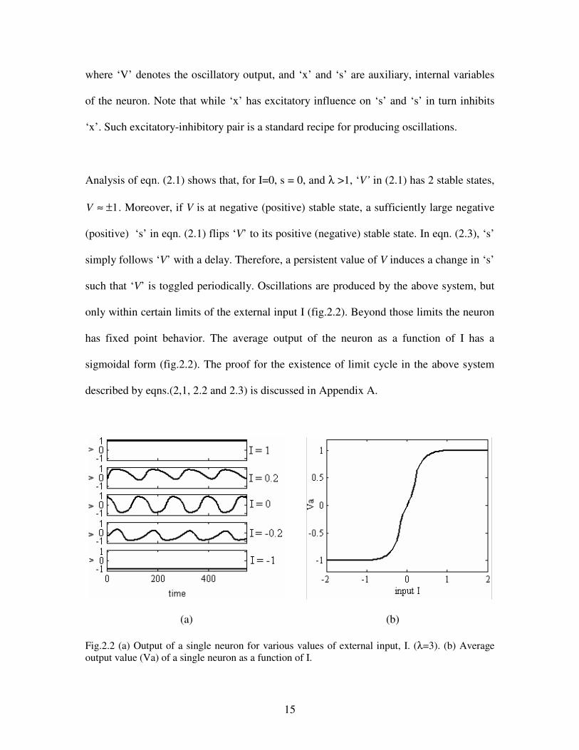
where ‘V’ denotes the oscillatory output, and ‘x’ and ‘s’ are auxiliary, internal variables
of the neuron. Note that while ‘x’ has excitatory influence on ‘s’ and ‘s’ in turn inhibits
‘x’. Such excitatory-inhibitory pair is a standard recipe for producing oscillations.
Analysis of eqn. (2.1) shows that, for I=0, s = 0, and λ >1, ‘V’ in (2.1) has 2 stable states,
1V ≈ ± . Moreover, if V is at negative (positive) stable state, a sufficiently large negative
(positive) ‘s’ in eqn. (2.1) flips ‘V’ to its positive (negative) stable state. In eqn. (2.3), ‘s’
simply follows ‘V’ with a delay. Therefore, a persistent value of V induces a change in ‘s’
such that ‘V’ is toggled periodically. Oscillations are produced by the above system, but
only within certain limits of the external input I (fig.2.2). Beyond those limits the neuron
has fixed point behavior. The average output of the neuron as a function of I has a
sigmoidal form (fig.2.2). The proof for the existence of limit cycle in the above system
described by eqns.(2,1, 2.2 and 2.3) is discussed in Appendix A.
(a) (b)
Fig.2.2 (a) Output of a single neuron for various values of external input, I. (λ=3). (b) Average
output value (Va) of a single neuron as a function of I.
16
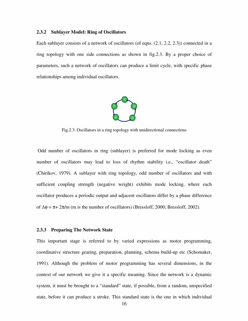
2.3.2 Sublayer Model: Ring of Oscillators
Each sublayer consists of a network of oscillators (of eqns. (2.1, 2.2, 2.3)) connected in a
ring topology with one side connections as shown in fig.2.3. By a proper choice of
parameters, such a network of oscillators can produce a limit cycle, with specific phase
relationships among individual oscillators.
Fig.2.3. Oscillators in a ring topology with unidirectional connections
Odd number of oscillators in ring (sublayer) is preferred for mode locking as even
number of oscillators may lead to loss of rhythm stability i.e., “oscillator death”
(Chirikov, 1979). A sublayer with ring topology, odd number of oscillators and with
sufficient coupling strength (negative weight) exhibits mode locking, where each
oscillator produces a periodic output and adjacent oscillators differ by a phase difference
of ∆φ = π+ 2π/m (m is the number of oscillators) (Bressloff, 2000; Bressloff, 2002).
2.3.3 Preparing The Network State
This important stage is referred to by varied expressions as motor programming,
coordinative structure gearing, preparation, planning, schema build-up etc (Schomaker,
1991). Although the problem of motor programming has several dimensions, in the
context of our network we give it a specific meaning. Since the network is a dynamic
system, it must be brought to a “standard” state, if possible, from a random, unspecified
state, before it can produce a stroke. This standard state is the one in which individual
17
oscillators of a sublayer are brought to target phases (φ1, …, φi,…, φn) by the time the
network is ready for stroke execution. This preparation is achieved by giving a
Preparatory Pulse (PP) to a specific neuron (chosen to be the 1st neuron in every sublayer
without loss of generality) and waiting for a specific delay interval. The delay must be
long enough to allow the oscillatory layer to approach the limit cycle sufficiently closely;
beyond this minimum value the delay must be precisely chosen such that the oscillatory
layer state is at a predetermined phase in the limit cycle. We refer to this state as the
“standard state” henceforth. Thus, by proper choice of pulse (its duration, τ, and
amplitude, A) and the delay, ∆, (elapsed after the PP and before the stroke execution
begins) the network can be brought to the desired state (V=[V1, …, Vi,…, Vn]) with
sufficient accuracy.
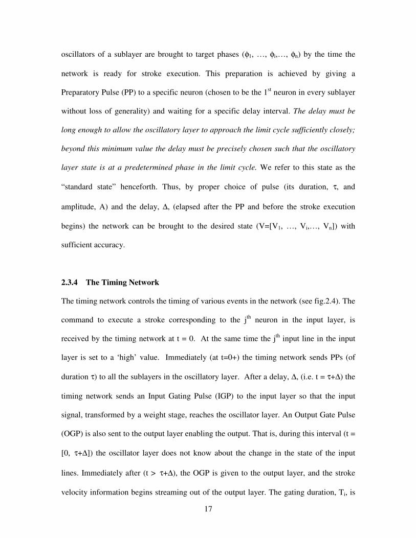
2.3.4 The Timing Network
The timing network controls the timing of various events in the network (see fig.2.4). The
command to execute a stroke corresponding to the jth
neuron in the input layer, is
received by the timing network at t = 0. At the same time the jth
input line in the input
layer is set to a ‘high’ value. Immediately (at t=0+) the timing network sends PPs (of
duration τ) to all the sublayers in the oscillatory layer. After a delay, ∆, (i.e. t = τ+∆) the
timing network sends an Input Gating Pulse (IGP) to the input layer so that the input
signal, transformed by a weight stage, reaches the oscillator layer. An Output Gate Pulse
(OGP) is also sent to the output layer enabling the output. That is, during this interval (t =
[0, τ+∆]) the oscillator layer does not know about the change in the state of the input
lines. Immediately after (t > τ+∆), the OGP is given to the output layer, and the stroke
velocity information begins streaming out of the output layer. The gating duration, Ti, is
18
specific to the stroke that is being produced and is presently equal to the time period, Tf,
of the slowest oscillators (those of first sublayer) in the oscillatory layer. We will relax
this condition in future section and study its consequences. A summary of events in fig.
2.4 are shown in table 2.1:
Fig.2.4.The timing signals (PP: Preparatory Pulse, IGP: Input Gate Pulse, OGP: Output Gate
Pulse), A is the amplitude of preparatory pulse, ‘τ’ is the duration of PP, Ti is the duration of OGP
for ith
stroke and ‘∆’ is the delay. The Post preparatory delay is given by (PPD) the sum τ+∆ time
units.
Table.2.1. Summary of events in handwriting generation
Events Event Summary
A The input is fed to the network (also to timing network). The timing network
injects PP for the duration (τ), to the 1st oscillator in every sublayer. Input to
the oscillatory network is disabled during this interval since the IGP is low.
B This event is the end of PP and start of delay for duration ∆. IGP and OGP
continues to be low.
C Start of IGP and OGP with duration Ti, which enable the input and output. The
network starts generating velocity information.
D The end of IGP and OGP, the network is again disabled, velocities become
zero, and the pen tip stops.
A
ττττ
∆∆∆∆
PP
IGP
A B C D
Ti
Events
1 0 1 0 OGP
19
Fig.2.5. Dynamics of the oscillators network during preparation. The oscillator layer has 6
sublayers with 25 oscillators for each sublayer. GP represents both IGP and OGP. The PP is given
from zero time units to 20 time units. The GP is brought up from 620 time units onwards.
Fig.2.6. Cartoon of state space illustrating trajectories in preparation and execution of a
movement. Average firing rates of neurons n1, n2 and n3 are shown along the axes. The initial
activity of the neurons is near the origin (shown as one small circle per trial). Following target
onset, activity of neurons settles (through curved paths) to a subspace of states appropriate for the
desired movement (volume inside the shaded region). The standard state is part of this subspace.
n1
n2
n3
Nearly standard
Random initial States
Preparation
Execution of the movement
Trajectories of network state corresponding to ‘Ballistic movements’
20
The dynamics of the network along with Gate Pulse, GP (is shown considering IGP =
OGP) and PP during preparation are shown in fig.2.4. A PP signal is given at the
beginning of the session. The onset of handwriting movement starts at GP. Note that
there is ‘mode locking’ in each sublayer towards end of preparation delay. The onset of
GP or handwriting movement occurs at the registry of standard state (at time units 620 in
fig.2.5). The more details on ‘time unit’ are discussed in section 5.1 of chapter 5.
The fig.2.6 explains the events of the network in terms of network’s state and trajectory
followed by the state. The trajectory from the initially variable state (near the base line;
shown as one dot per trial) to standard state (states in shaded volume shape in fig.2.6)
corresponds to preparation of the network. Different trajectories emanating from the
standard state leads to various movements. Note that all trajectories corresponding to
variable initial states go through the standard state, which is the essence of preparation.
2.3.5 Network Response
Pen-tip velocities (Ux and Uy) estimated by the network are expressed as weighted
sum of the outputs of the oscillator layer:
)()(1 1
tVWtU ik
Ns
k
Nk
i
x
ikx ∑∑= =
= (2.4)
)()(1 1
tVWtU ik
Ns
k
Nk
i
y
iky ∑∑= =
= (2.5)
where, Ns is the number of sublayers in the oscillatory layer and Nk is the number of
oscillator in kth
sublayer, Wxik and W
yik are connections from i’th oscillator in k’th sublayer
to output nodes Ux and Uy respectively. Output, Vik, of the i’th oscillator in the k’th
sublayer is given by:
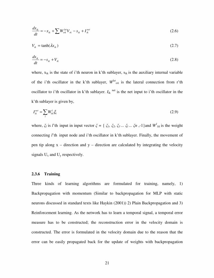
21
net
ikikrk
lat
irkik
ik IsVWxdt
dx+−+−= ∑ (2.6)
)tanh( ikik xV λ= (2.7)
ikik
ik Vsdt
ds+−= (2.8)
where, xik is the state of i’th neuron in k’th sublayer, sik is the auxiliary internal variable
of the i’th oscillator in the k’th sublayer, Wlat
irk is the lateral connection from r’th
oscillator to i’th oscillator in k’th sublayer. Iik net
is the net input to i’th oscillator in the
k’th sublayer is given by,
1net
ik lik l
l
I W ξ=∑
(2.9)
where, ξl is l’th input in input vector ξ = { ξ1, ξ2, ξ3 ... ξl ... ξn ,-1}and W
1lik is the weight
connecting l’th input node and i’th
oscillator in k’th
sublayer. Finally, the movement of
pen tip along x – direction and y – direction are calculated by integrating the velocity
signals Ux and Uy respectively.
2.3.6 Training
Three kinds of learning algorithms are formulated for training, namely, 1)
Backpropagation with momentum (Similar to backpropagation for MLP with static
neurons discussed in standard texts like Haykin (2001)) 2) Plain Backpropagation and 3)
Reinforcement learning. As the network has to learn a temporal signal, a temporal error
measure has to be constructed; the reconstruction error in the velocity domain is
constructed. The error is formulated in the velocity domain due to the reason that the
error can be easily propagated back for the update of weights with backpropagation
22
algorithm. If the error is constructed in spatial domain the error needs to be differentiated
and hence formulation of backpropagation algorithm becomes tedious.
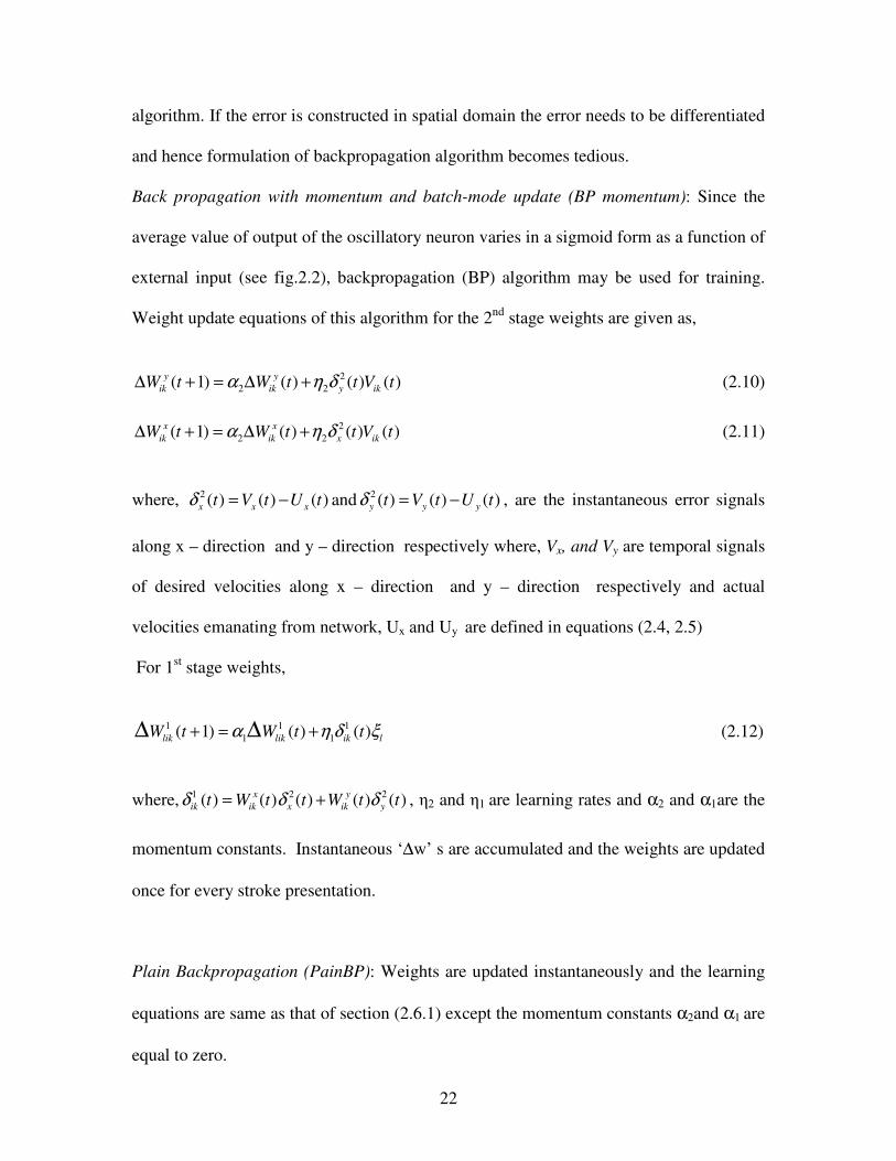
Back propagation with momentum and batch-mode update (BP momentum): Since the
average value of output of the oscillatory neuron varies in a sigmoid form as a function of
external input (see fig.2.2), backpropagation (BP) algorithm may be used for training.
Weight update equations of this algorithm for the 2nd
stage weights are given as,
2
2 2( 1) ( ) ( ) ( )y y
ik ik y ikW t W t t V tα η δ∆ + = ∆ + (2.10)
2
2 2( 1) ( ) ( ) ( )x x
ik ik x ikW t W t t V tα η δ∆ + = ∆ + (2.11)
where, 2 ( ) ( ) ( )x x x
t V t U tδ = − and 2 ( ) ( ) ( )y y yt V t U tδ = − , are the instantaneous error signals
along x – direction and y – direction respectively where, Vx, and Vy are temporal signals
of desired velocities along x – direction and y – direction respectively and actual
velocities emanating from network, Ux and Uy are defined in equations (2.4, 2.5)
For 1st stage weights,
1 1 1
1 1( 1) ( ) ( )lik lik ik l
W t W t tα η δ ξ+ = +∆ ∆ (2.12)
where, 1 2 2( ) ( ) ( ) ( ) ( )x y
ik ik x ik yt W t t W t tδ δ δ= + , η2 and η1 are learning rates and α2 and α1are the
momentum constants. Instantaneous ‘∆w’ s are accumulated and the weights are updated
once for every stroke presentation.
Plain Backpropagation (PainBP): Weights are updated instantaneously and the learning
equations are same as that of section (2.6.1) except the momentum constants α2and α1 are
equal to zero.
23
Reinforcement learning(RL): The network is also tested with reinforcement learning
(Barto, 1999; Hertz, 1991) for the 1st stage weights, and is given as,
1
( 1) ( )W t V tlik ik l
η ξ+ =+
∆ if e ≤ ε (2.13)
1( 1) ( )W t V t
lik ik lη ξ+ =
−∆ if e > ε (2.14)
where, η+ (η− )is small positive(negative) constant, ‘e’ is the output error, and ε is the
error threshold for reward-based learning. The second layer update equations are
formulated using gradient descent method similar to backpropagation algorithm. The
equation for weight update 2nd
stage is the same as that of back propagation of error given
as in eqn (2.10 and 2.11) with α2and α1 being equal to zero.
Calculation of mean reconstruction error: The reconstruction error of pth
stroke is given
by the formula as,
{ }2 2( ( ) ( )) ( ( ) ( ))Nl
p p p p p
q q q q
q
E Vx t Ux t Vy t Uy t= − + −∑ (2.15)
And the mean error of all strokes is given by,
Nsp
p
E
ENs
=∑
(2.16).
Where, Ns is the number of strokes and Nl is the number of points in velocity profile of
pth
stroke. And ( )p
xV t and ( )p
yV t are the desired velocity profiles of the pen tip which are
collected using a stylus connected to computer. More details about the data collection are
discussed in chapter 5. The mean reconstruction error defined in eqn.2.16 is compared
over several trials for the training algorithms discussed above (see fig2.7). BP with
24
momentum found to be faster and efficient compared to the other two algorithms (see
fig.2.7). The samples reconstructed strokes are shown in fig2.8.
Fig.2.7. Comparison of three kinds of learning algorithms (Plain BP, BP with momentum,
Reinforcement learning (RL)). The mean error for “BP with momentum and batch-mode update”
converges faster than other two learning mechanisms.
Fig. 2.8. Reconstructed strokes ‘a’ and ‘k’. The dynamics of oscillatory layer along with the
stroke velocity profiles are shown. On left side original stroke and corresponding velocity profiles
and to right side velocities generated and strokes reconstructed are shown.
25
2.4 SUMMARY
In the present chapter a model of handwriting generation based on Fourier style
reconstruction is discussed. The model is further investigated to optimize several aspects
of the network like assignment of frequencies of oscillator sublayers, size of the oscillator
layer, multiple stroke production etc. These experiments along with results are discussed
in detail in chapter 5. The current model can be mapped on to neuroanatomy; the ‘timing
network’ which controls the events in the main network, resembles BG. BG is known to
have a role in timing and preparation of SMA and PM activity in executing a motor
activity. More details of mapping of the current model onto neuroanatomy are discussed
in chapter 6. Next chapter discusses about the BG and its functional roles along with a
model. It is shown in the next chapter that apart from functional roles like timing and
preparation, BG has a role in reinforcement learning.
26
CHAPTER 3
BASAL GANGLIA AS A SOURCE OF EXPLORATORY DRIVE:
A MODEL FOR REACHING
Any act which in a given situation produces satisfaction becomes associated with that situation so
that when the situation recurs the act is more likely than before to recur also.
– E.L. Thorndike (1911)
3.1 BASAL GANGLIA
3.1.1 Neuroanatomy of Basal Ganglia
BG receive inputs from most of the sensory motor areas of the cerebral cortex, including
primary and secondary somatosensory areas, primary motor cortex (M1) and a variety of
premotor areas, including supplementary area, the dorsal and ventral premotor areas. The
anatomical basis of motor functions of BG is illustrated in fig. 3.1. The portions of cortex
which are responsible for movement SMA, PM, M1, somatosensory cortex, and the
superior parietal lobule make dense, topographically organized projections to the motor
portion of Putamen (input nuclei of BG). The output of this pathway, termed the motor
circuit of the BG, is directed primarily back to the SMA and PM cortex. These areas are
reciprocally interconnected with each other and with motor cortex and all have direct
descending projections to brain stem motor centers and spinal cord.
BG consists of five extensively connected subcortical nuclei: the caudate nucleus,
putamen, globus pallidus, subthalamic nucleus (STN), and substantia nigra (pars
Compacta SNc, and pars reticula SNr). Caudate and Putamen are together named as STR
which is the input nuclei of the BG. Most striatal neurons are medium spiny and have
GABAergic projections. Globus Pallidus can be divided into two parts namely Globus
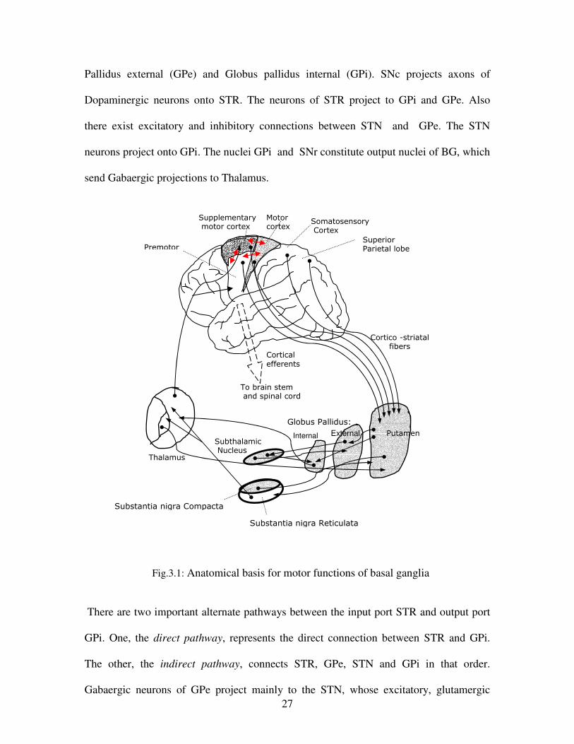
27
Pallidus external (GPe) and Globus pallidus internal (GPi). SNc projects axons of
Dopaminergic neurons onto STR. The neurons of STR project to GPi and GPe. Also
there exist excitatory and inhibitory connections between STN and GPe. The STN
neurons project onto GPi. The nuclei GPi and SNr constitute output nuclei of BG, which
send Gabaergic projections to Thalamus.
Fig.3.1: Anatomical basis for motor functions of basal ganglia
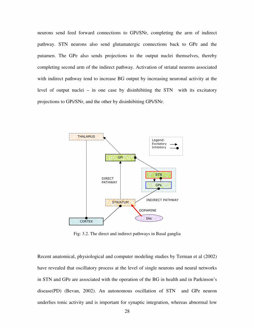
There are two important alternate pathways between the input port STR and output port
GPi. One, the direct pathway, represents the direct connection between STR and GPi.
The other, the indirect pathway, connects STR, GPe, STN and GPi in that order.
Gabaergic neurons of GPe project mainly to the STN, whose excitatory, glutamergic
Putamen Internal Subthalamic Nucleus
Thalamus
To brain stem and spinal cord
Premotor
Supplementary motor cortex
Motor cortex
Somatosensory Cortex
Superior Parietal lobe
Cortico -striatal fibers
Cortical efferents
External
Globus Pallidus:
Substantia nigra Compacta
Substantia nigra Reticulata
28
neurons send feed forward connections to GPi/SNr, completing the arm of indirect
pathway. STN neurons also send glutamatergic connections back to GPe and the
putamen. The GPe also sends projections to the output nuclei themselves, thereby
completing second arm of the indirect pathway. Activation of striatal neurons associated
with indirect pathway tend to increase BG output by increasing neuronal activity at the
level of output nuclei – in one case by disinhibiting the STN with its excitatory
projections to GPi/SNr, and the other by disinhibiting GPi/SNr.
Fig: 3.2. The direct and indirect pathways in Basal ganglia
Recent anatomical, physiological and computer modeling studies by Terman et al (2002)
have revealed that oscillatory process at the level of single neurons and neural networks
in STN and GPe are associated with the operation of the BG in health and in Parkinson’s
disease(PD) (Bevan, 2002). An autonomous oscillation of STN and GPe neuron
underlies tonic activity and is important for synaptic integration, whereas abnormal low
GPi
STN
GPe
THALAMUS
STRIATUM
CORTEX
INDIRECT PATHWAY
DIRECT PATHWAY
SNc
DOPAMINE
Legend: Excitatory
Inhibitory
29
frequency rhythmic bursting in the STN and GPe is characteristic of PD. Normal
information processing is characterized by complex spatiotemporal patterns of firing,
whereas in PD, STN and GPe neurons display more correlated synchronous and rhythmic
activity (Bevan, 2002; Bergman, 1998). The obvious question that arises is, “what is the
functional significance of these complex oscillations?” In this chapter an attempt is made
based on a computational model of BG. It is argued that the complex activity of BG acts
as a source of exploratory drive. The subsequent sections emphasize reward signaling in
BG and realization of reinforcement signal.
3.1.2 Reward Signaling in Basal Ganglia: How does Reward Lead to Learning?
Dopaminergic inputs to the putamen consist of nigrostriatal projections that originate in
the SNc. At the network level dopamine appears to have different role in the direct and
indirect pathway. Given the reciprocal reentrant effects associated with differential
activations of the direct versus the indirect pathways, the differential effects of dopamine
on these two pathways would be viewed as resulting in the enhancement of positive
feedback, and suppression of negative feedback, returned to the various cortical areas that
receive BG influences (Alexander, 1998).
Dopamine has also been shown to have a role in synaptic plasticity within the STR, being
implemented in both Long term Potentiation (LTP) and Long term Depression (LDP).
Dopamine neurons may play an important role in determining when striatal neurons
should be strengthened or weakened. In this respect Dopamine might be seen as playing a
role in striatal information processing, analogous to “adaptive critic” in connectionist
networks.
30
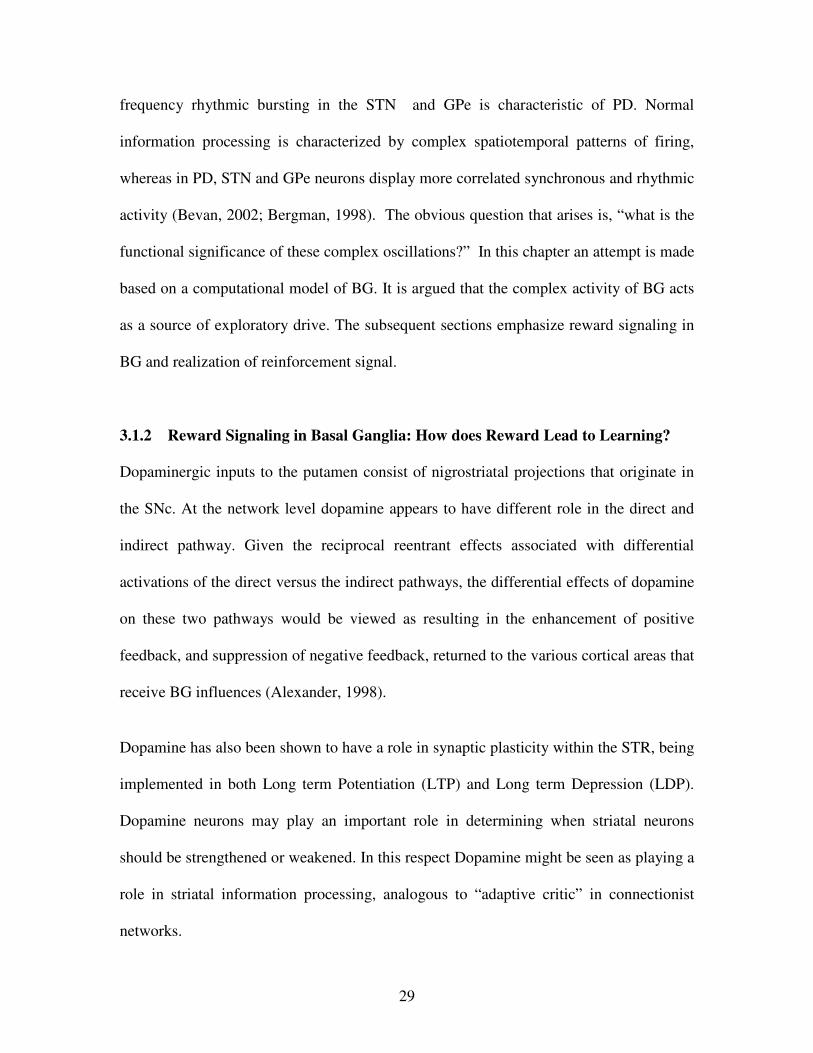
Fig. 3.3 How rewards lead to learning? Steps involved in reward based learning5. See text for the
explanation of these steps.
Currently a widely accepted view is that the input from dopaminergic neurons to the STR
provides the reinforcement signal required for adjusting the probabilities of subsequent
action selection. Positive reinforcement helps to control the acquisition of learned
behaviors (Reynolds et al, 2001). Reynolds et al (2001) report a cellular mechanism in
the brain that may underlie the behavioral effects of positive reinforcement. They have
used intracranial self-stimulation (ICSS) as a model of reinforcement learning, in which
each rat learns to press a lever that applies reinforcing electrical stimulation to its own
substantia nigra. With experiments on Intra Cranial Self Stimulation (ICSS) model of
reinforcement learning, they explain how rewards could lead to learning (see fig.3.3).
5 Figure taken from url: http://anatomy.otago.ac.nz/research/basal-
ganglia/publications/abstracts/2001_nature.html 7 This part of the discussion is heavily drawn from the excellent review article on Computational
Approaches to Neurological Diseases by Crystal and Finkel in the book, Reggia, Ruppin and Berndt,
Neural Modeling of Brain and Cognitive disorders, World Scientific, 1996.
31
Steps involved in reward based learning in BG: 1. Cells within the brain involved in generating movement are activated and send their output to
STR.
2. Other brain areas decide if the movement produced an outcome that was rewarding and send
the result to the dopamine cells.
3. If the result is interpreted as “good,” the dopamine cells are activated and release a pulse of
dopamine into the STR.
4. The released dopamine causes connections within those circuits which were active in the
production of the movement to be strengthened.
5. The reinforcement of the connections between neurons induced by dopamine is long – lasting.
Next time, the same situation is much more likely to produce the same movement response
(Reynolds, 2001).
The current model of BG is based on RL, draws the above mentioned steps to some
extent. Any realization of reinforcement learning requires, in addition to a reward signal,
a noise source that can exhaustively explore the output (or action space). It is proposed in
this chapter that the complex activity of STN – GPe loop accounts for the noise signal.
3.2 COMPUTATIONAL MODELS OF BASAL GANGLIA
Enormous progress has been made in characterizing the structure and functionality of the
BG, and yet comprehensive understanding of the contribution of these nuclei to
behavioral control remains elusive. Functional models of BG are thus in great need for a
comprehensive theory of BG operations. Functional models should be able to both
assimilate the constraints imposed by the neurobiological data and to simulate various
candidate behavioral functions in which these structures (nuclei) are believed to
participate (Alexander, 1998). Computational modeling of neurons and neural networks
is complementary to traditional techniques in neuroscience (Houk et al, 1998). Thus
computational modeling of BG based on neurobiological data is significant for
comprehensive understanding. In this section a brief review of computational models of
BG highlighting its functional roles is presented. This effort has drawn heavily from the
excellent reviews presented by Prescott et al (2003) and Houk et al (1998).
32
Most of the effort so far directed at BG modeling has been concerned with simulating
interactions between the various BG structures, and between the BG and other key brain
regions such as cortex, thalamus, and brain stem (Prescott et al 2003). The chief
computational hypotheses governing the BG model investigate the following functions:
i. Regulation of the degree of action gating
ii. Selection between competing actions
iii. Sustaining working memory representations
iv. Storing and enhancing sequences of behavior
v. Reinforcement learning
vi. Timing and coincidence detection
Action Gating
A key function of the STR is to provide intermittent, focused inhibition (via the ‘direct
pathway’) within output structures which otherwise maintain inhibitory control over
motor/cognitive systems throughout the brain. This architecture strongly suggests that a
core function of BG is to gate the activity of target system via the mechanism of
disinhibiting. Many BG models employ selective gating, however that of Vidal and
Stelmach (1995) is interesting as it explores gating operations in both normal and
dysfunctional model variants. These authors coupled a simulation of BG intrinsic
circuitry to a neural network (Bullock’s VITE model) that computed arm movements.
Excitatory striatal input resulted in a smoothly varying signal to thalamic targets that
provided ‘GO’ signal for the motor command, and also sets its overall velocity. The time
taken to execute movements decreased with increasing BG input thereby matching the
33
results of striatal micro stimulation studies. A ‘dopamine depleted’ version of the model
exhibited akinesia and bradykinesia similar to that observed in Parkinson’s disease.
Selecting Between Competing Actions
The proposal that the BG acts to resolve action selection competition is based on a
growing consensus that a key function of these structures to arbitrate between sensory
motor systems competing for access to the final common motor path. A computational
hypothesis developed from this idea relies on the premise that afferent signals to the STR
encode the salience of ‘requests for the action’ to the motor system (Redgrave et al,
1999). Multiple selection mechanisms embedded in BG could resolve conflict between
competitors and provide clean rapid switching between winners. First, the up/down states
of the striatal neurons may act as a first pass filter to exclude weakly supported
‘requests’. Second, local inhibition within the STR could selectively enhance the activity
of the most salient channel. Third, the combination of focused inhibition from STR with
diffused excitation from STN could operate as a feed forward, off-center/on surround
network across the BG as a whole (Mink, 1996). Lastly, local reciprocal inhibition within
the output nuclei could sharpen up the final selection. An earlier model of Berns and
Sejnowski (1996) shared the ‘action selection’ premise of Gurney et al (2001), but
emphasized possible timing differences between the direct and indirect pathways in a
model that included just the feed-forward intrinsic BG connections. An interesting feature
of this model is that it incorporated a version of the dopamine hypothesis for
reinforcement learning as a means for adaptively tuning the selection mechanism.
34
Sustaining Working Memory
The relationship between BG and cortex is characterized by segregated parallel loops, in
which cortical projections to the STR are channeled through BG outputs to the thalamus
and then back to their cortical areas of origin. The thalamic nuclei in this circuit have
reciprocal, net excitatory, connections to their cortical targets. This architecture suggests
a pattern of cortical thalamic activity which, once initiated by disinhibitory signals from
BG, could be sustained indefinitely. Several authors proposed that this circuit would act
as a working memory store (e.g.: Houk et al., 1995)
Sequence Learning
A plausible use for the working memory mechanism outlined in the previous section
would be to link successful selection during the development of behavioral / cognitive
sequences. This idea has therefore become a central theme in a number of BG models.
For example, Berns and Sejnowski (1998) propose a systems level computational model
of the BG based closely on known anatomy and physiology. They assume that the
thalamic targets, which relay ascending information to cortical action and planning areas,
are tonically inhibited by the BG. Another assumption is that the output stage of the BG,
GPi, selects a single action from several competing actions via lateral interactions.
Finally they propose that a form of local working memory exists in the form of reciprocal
connections between the external GPe and STN, with the STN-GPe connections learning
by an associative learning rule. Thus the STR, which was assumed to be a conjunction of
cortical states directly, selects an action from GPe during training which, after training is
complete, acts as a cue for the production of the complete sequence of actions, thereby
35
providing a mechanism for encoding action sequences. Sequence learning is another
important issue in BG modeling. For instance Dominey (1995) have extended their model
of delayed saccade control to include a mechanism for associative and sequence learning
based, again, on the hypothesis that dopamine provides a reinforcement learning signal.
Reinforcement Learning
The term “Reinforcement Learning(RL)” comes from the studies of animal learning in
experimental psychology, where it refers to the occurrence of an event, in a proper
relation to a response, that tends to increase the probability the response will occur again
in the same situation (Barto, 1998). The term RL is widely adopted by theorists in
engineering and artificial intelligence. It is usually formulated as an optimization problem
with the objective of finding an action or strategy for producing an action that is optimal
or best in some well-defined way. Most of the models of reinforcement learning are
based on actor–critic architecture wherein critic sends reinforcement to actor in response
to an action made by it. There exists non – associative and associative reinforcement
learning in the literature. In non – associative learning, the only input to the learning
system is reinforcement signal, whereas in associative case the learning system also
receives stimulus process that provides information about the process and possibly other
information as well. In both the cases following are the key observations suggested by
Barto (1998).
1. Uncertainty plays a key role in the RL.
2. The critic is an abstract model that evaluates the learning system’s actions.
3. The reinforcement signal can be any signal evaluating the learning system’s actions.
36
4. The critic’s signal does not does not directly tell the leaning system what action is the
best; it only evaluates the action taken.
5. RL algorithms are selection processes.
6. RL involves a conflict between exploitation and exploration.
The increased interest in RL is due to its applicability to learning by autonomous robotic
agents, and hence a number of models and learning algorithms have evolved. Some of
these are listed below.
1. Classical conditioning
a. Roscorla Wagner rule: It is based on “theory of Pavlovian conditioning” (Roscorla
and Wagner, 1972) for the prediction of reward.
b. Predicting future reward by Temporal Difference Learning Rule (TDRL).
The prediction error (δ )� plays an important role in both of the above learning rules.
Schultz et al (1998) and Montague et al (1996) recognized that dopaminergic neurons in
SNc and ventral tegmental area (VTA) carry a (dopamine) signal that encodes
prediction error.
2. Associative RL rules
a. Associative search rule (Klopf, 1982): It is basically hebbian correlation rule with
the reinforcement signal acting as a modulatory factor.
b. Selective bootstrap (Widrow et al, 1973): It is an extension of LMS rule.
c. Associative reward penalty (ARP) (Barto and Anandan, 1985): This can be
realized with essential ingredients as stochastic output units. In terms of cost
function as there is no gradient information, it is important to have randomness in
the learning system, so that possible outputs can be explored until a correct
(rewarding) output is found.
37
3. Sequential action choice
Sequential reinforcement requires improving the long – term consequences of action,
or of a strategy for performing actions, in addition to short-term consequences. An
important special case of this problem occurs when there is no immediate
reinforcement until a goal state is reached. Samuels checkers player, Sutton’s
temporal difference TD methods(1988), Tesauro’s backgammon(1992), Watkin’s
Q- learning(1989) comes under this category.
There is considerable evidence that the dopaminergic neurons which project from the
midbrain to the neostriatum mediate an internal reinforcement signal. A major target of
this signal is the synapses that connect the cerebral cortex to neostriatum. However the
effect of dopamine on these synapses is not completely understood (Wickens, 1998;
Barto, 1998). Is has been shown that dopamine has positive reinforcement on striatal
neurons. A model based on corticostriatal interactions, in which modifiable synapses
located in the corticostriatal pathway, promises to be a useful way of integrating cellular
mechanisms of reinforcement into intelligent behavior.
Timing and Coincidence Detection
Coordinating the relative timing of multiple streams of processing is crucial in both
motor performance and sensory perception. Temporal processing in biological systems
occurs over a range of time scales and is broadly classified into 3 categories: 1) circadian
timing, which corresponds durations of the order of days, and handled by brain structures
like suprachiasmatic nuclei, 2) interval timing, which corresponds to durations in the
range of seconds to minutes, and coordinated primarily by corticostriatal interactions, and
38
3) millisecond timing, which obviously corresponds to millisecond durations, controlled
by the cerebellum (Buhusi and Meck, 2005).
The role of BG in ‘interval timing’ appears to emerge from the dynamics of thalamo-
cortico-striatal loops. In the Striatal Beat Frequency (SBF) model (Buhusi and Meck,
2005), a model that highlights the timing function of BG, the cortical oscillators are
assumed to increase synchrony just before movement onset and maintain the rhythm
throughout the performance. The dopaminergic burst at trial onset could trigger the
synchronization of cortical oscillators according to SBF model(Buhusi and Meck, 2005)
and the striatal neurons are tuned to respond to specific patterns of cortical oscillations
(Buhusi and Meck, 2005).
Apart from the above conceptual additions to knowledge on BG’s functional significance,
it is known to have a role in cognitive and memory operations (Houk et al, 1998). BG
model is still in the stage of exploring the space of alternative hypothesis, seeking to
rationalize theoretical proposals whilst trying to match known neurological constraints
(Prescott et al, 1999). We hence propose a model of BG in the next section with specific
neurobiological analogs.
3.3 PRESENT MODEL
The present model is based on the hypothesis that the dopamine signal that encodes
reward for an action, selects the pathways in BG to coerce the animal into exploration or
exploitation for a given situation. For the purpose of simulating the above hypothesis, a
task based model is assumed wherein the BG learns to persuade a 2-joint model of arm to
reach a target.
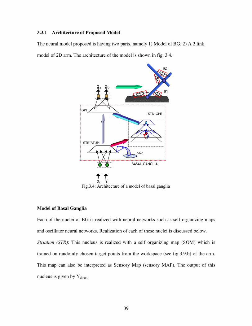
39
3.3.1 Architecture of Proposed Model
The neural model proposed is having two parts, namely 1) Model of BG, 2) A 2 link
model of 2D arm. The architecture of the model is shown in fig. 3.4.
Fig.3.4: Architecture of a model of basal ganglia
Model of Basal Ganglia
Each of the nuclei of BG is realized with neural networks such as self organizing maps
and oscillator neural networks. Realization of each of these nuclei is discussed below.
Striatum (STR): This nucleus is realized with a self organizing map (SOM) which is
trained on randomly chosen target points from the workspace (see fig.3.9.b) of the arm.
This map can also be interpreted as Sensory Map (sensory MAP). The output of this
nucleus is given by Ydirect.
STN-GPE GPI
θ2
θ1 ga gb
BASAL GANGLIA
STRIATUM
SNc
Xt Yt
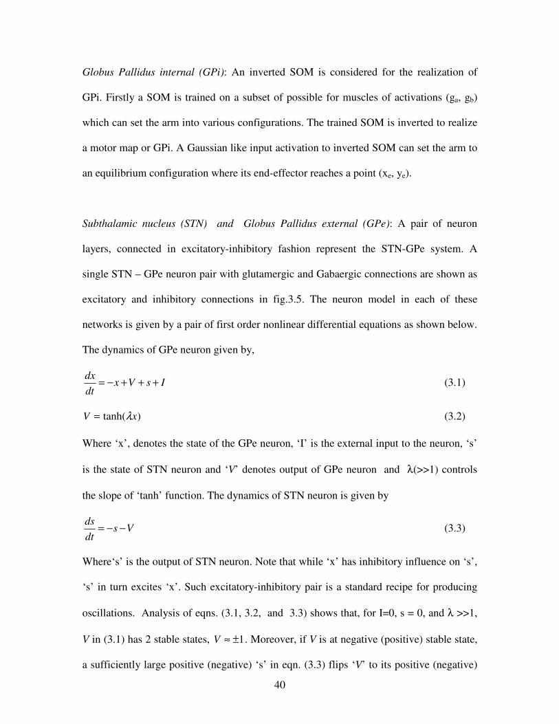
40
Globus Pallidus internal (GPi): An inverted SOM is considered for the realization of
GPi. Firstly a SOM is trained on a subset of possible for muscles of activations (ga, gb)
which can set the arm into various configurations. The trained SOM is inverted to realize
a motor map or GPi. A Gaussian like input activation to inverted SOM can set the arm to
an equilibrium configuration where its end-effector reaches a point (xe, ye).
Subthalamic nucleus (STN) and Globus Pallidus external (GPe): A pair of neuron
layers, connected in excitatory-inhibitory fashion represent the STN-GPe system. A
single STN – GPe neuron pair with glutamergic and Gabaergic connections are shown as
excitatory and inhibitory connections in fig.3.5. The neuron model in each of these
networks is given by a pair of first order nonlinear differential equations as shown below.
The dynamics of GPe neuron given by,
dxx V s I
dt= − + + + (3.1)
)tanh( xV λ= (3.2)
Where ‘x’, denotes the state of the GPe neuron, ‘I’ is the external input to the neuron, ‘s’
is the state of STN neuron and ‘V’ denotes output of GPe neuron and λ(>>1) controls
the slope of ‘tanh’ function. The dynamics of STN neuron is given by
dss V
dt= − − (3.3)
Where‘s’ is the output of STN neuron. Note that while ‘x’ has inhibitory influence on ‘s’,
‘s’ in turn excites ‘x’. Such excitatory-inhibitory pair is a standard recipe for producing
oscillations. Analysis of eqns. (3.1, 3.2, and 3.3) shows that, for I=0, s = 0, and λ >>1,
V in (3.1) has 2 stable states, 1V ≈ ± . Moreover, if V is at negative (positive) stable state,
a sufficiently large positive (negative) ‘s’ in eqn. (3.3) flips ‘V’ to its positive (negative)
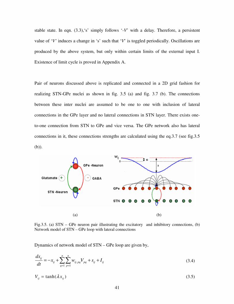
41
stable state. In eqn. (3.3),‘s’ simply follows ‘-V’ with a delay. Therefore, a persistent
value of ‘V’ induces a change in ‘s’ such that ‘V’ is toggled periodically. Oscillations are
produced by the above system, but only within certain limits of the external input I.
Existence of limit cycle is proved in Appendix A.
Pair of neurons discussed above is replicated and connected in a 2D grid fashion for
realizing STN-GPe nuclei as shown in fig. 3.5 (a) and fig. 3.7 (b). The connections
between these inter nuclei are assumed to be one to one with inclusion of lateral
connections in the GPe layer and no lateral connections in STN layer. There exists one-
to-one connection from STN to GPe and vice versa. The GPe network also has lateral
connections in it, these connections strengths are calculated using the eq.3.7 (see fig.3.5
(b)).
(a) (b)
Fig.3.5. (a) STN – GPe neuron pair illustrating the excitatory and inhibitory connections, (b)
Network model of STN – GPe loop with lateral connections
Dynamics of network model of STN – GPe loop are given by,
,
1 1
n nij
ij ij pq pq ij ij
q p
dxx w V s I
dt = =
= − + + +∑∑ (3.4)
tanh( )ij ij
V xλ= (3.5)
42
ij
ji ij
dss V
dt= − − (3.6)
where (i, j) and (p, q) denote the neurons position on the 2D grid, n is the size of the 2D
grid, xij is the state of (i, j) th
neurons on the GPe grid, sij is the state of (i, j) th
neurons on
the STN grid, Vij is the output of (i, j) th
neuron on the GPe network, Sij is the output of (i,
j) th
neuron on the STN network. The lateral connections, within GPe layer are assumed
to be translation invariant and are given by,
2 2
, exp( / )GPe
ij pq lat latW a rε σ= − − for r < R
= 0, otherwise. (3.7)
where rlat = [(i-p)2 + (j-q)
2]1/2
, squared distance of the neurons on 2D grid; ‘a’ controls
the depth of the Gaussian bell function and ‘σlat’ its width, and ‘R’ is the neighborhood
size. Thus each unit has a negative center and a positive surround; the relative sizes of
center and surround are determined by ε. Smaller ε implies, more negative lateral GPe
connections.
In the absence of input from the input layer (i.e., Iij = 0), as ε is varied from 0 to ‘a’, the
activity of STN-GPe system exhibits three different regimes: 1) chaos, 2) traveling
waves, and 3) clusters (see fig.3.6.). Similar dynamic behavior has also been observed in
more detailed electrophysiological models of STN-GPe system by Terman et al, 2002.
Operation of the network in the first regime – chaos – is most crucial since it is the
chaotic dynamics in the STN-GPe layer that makes the network extensively explore the
output space.
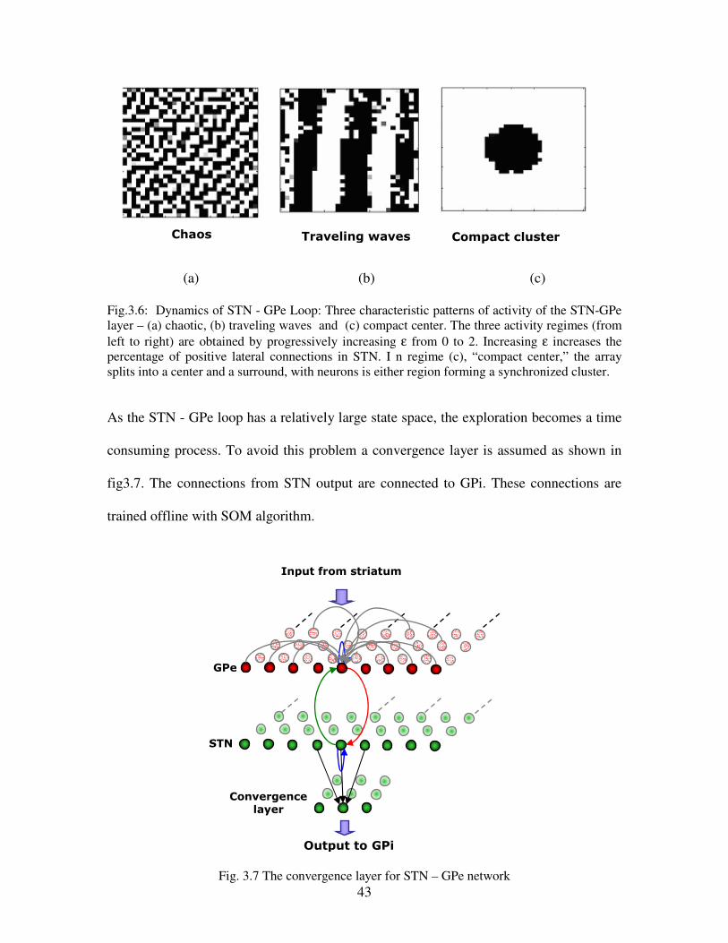
43
(a) (b) (c)
Fig.3.6: Dynamics of STN - GPe Loop: Three characteristic patterns of activity of the STN-GPe
layer – (a) chaotic, (b) traveling waves and (c) compact center. The three activity regimes (from
left to right) are obtained by progressively increasing ε from 0 to 2. Increasing ε increases the
percentage of positive lateral connections in STN. I n regime (c), “compact center,” the array
splits into a center and a surround, with neurons is either region forming a synchronized cluster.
As the STN - GPe loop has a relatively large state space, the exploration becomes a time
consuming process. To avoid this problem a convergence layer is assumed as shown in
fig3.7. The connections from STN output are connected to GPi. These connections are
trained offline with SOM algorithm.
Fig. 3.7 The convergence layer for STN – GPe network
Chaos Traveling waves
Output to GPi
Input from striatum
STN
GPe
Compact cluster
Convergence layer
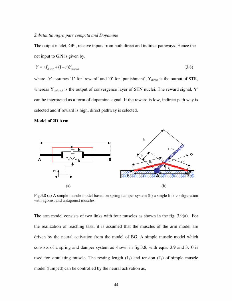
44
Substantia nigra pars compcta and Dopamine
The output nuclei, GPi, receive inputs from both direct and indirect pathways. Hence the
net input to GPi is given by,
(1 )direct indirect
Y rY r Y= + − (3.8)
where, ‘r’ assumes ‘1’ for ‘reward’ and ‘0’ for ‘punishment’, Ydirect is the output of STR,
whereas Yindirect is the output of convergence layer of STN nuclei. The reward signal, ‘r’
can be interpreted as a form of dopamine signal. If the reward is low, indirect path way is
selected and if reward is high, direct pathway is selected.
Model of 2D Arm
(a) (b)
Fig.3.8 (a) A simple muscle model based on spring damper system (b) a single link configuration
with agonist and antagonist muscles
The arm model consists of two links with four muscles as shown in the fig. 3.9(a). For
the realization of reaching task, it is assumed that the muscles of the arm model are
driven by the neural activation from the model of BG. A simple muscle model which
consists of a spring and damper system as shown in fig.3.8, with eqns. 3.9 and 3.10 is
used for simulating muscle. The resting length (Li) and tension (Ti) of simple muscle
model (lumped) can be controlled by the neural activation as,
θ1
h1
Link
P1 P2
x2
r r2 A
Q
l1
vi
A B k
b x
x1
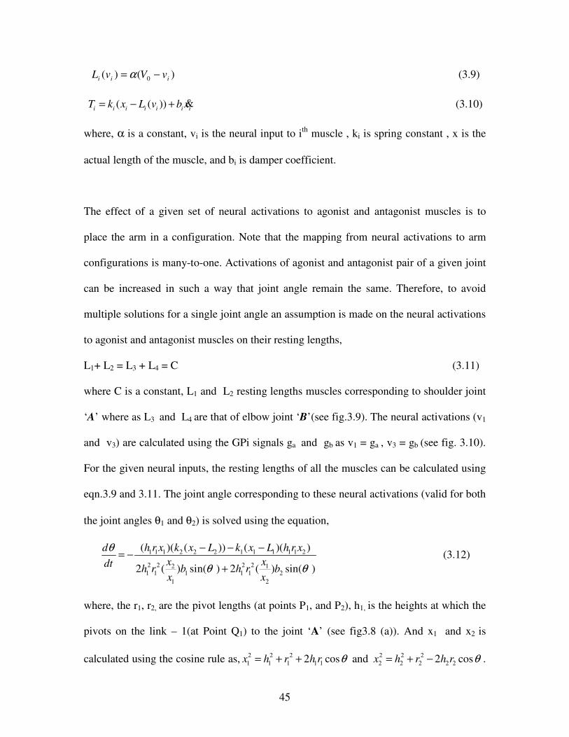
45
)()( 0 iii vVvL −= α (3.9)
( ( ))i i i i i i i
T k x L v b x= − + & (3.10)
where, α is a constant, vi is the neural input to ith
muscle , ki is spring constant , x is the
actual length of the muscle, and bi is damper coefficient.
The effect of a given set of neural activations to agonist and antagonist muscles is to
place the arm in a configuration. Note that the mapping from neural activations to arm
configurations is many-to-one. Activations of agonist and antagonist pair of a given joint
can be increased in such a way that joint angle remain the same. Therefore, to avoid
multiple solutions for a single joint angle an assumption is made on the neural activations
to agonist and antagonist muscles on their resting lengths,
L1+ L2 = L3 + L4 = C (3.11)
where C is a constant, L1 and L2 resting lengths muscles corresponding to shoulder joint
‘A’ where as L3 and L4 are that of elbow joint ‘B’(see fig.3.9). The neural activations (v1
and v3) are calculated using the GPi signals ga and gb as v1 = ga , v3 = gb (see fig. 3.10).
For the given neural inputs, the resting lengths of all the muscles can be calculated using
eqn.3.9 and 3.11. The joint angle corresponding to these neural activations (valid for both
the joint angles θ1 and θ2) is solved using the equation,
1 1 1 2 2 2 1 1 1 1 1 2
2 2 2 22 11 1 1 1 1 2
1 2
( )( ( )) ( )( )
2 ( ) sin( ) 2 ( ) sin( )
h r x k x L k x L h r xd
x xdth r b h r b
x x
θ
θ θ
− − −= −
+
(3.12)
where, the r1, r2, are the pivot lengths (at points P1, and P2), h1, is the heights at which the
pivots on the link – 1(at Point Q1) to the joint ‘A’ (see fig3.8 (a)). And x1 and x2 is
calculated using the cosine rule as, 2 2 2
1 1 1 1 12 cosx h r h r θ= + + and 2 2 2
2 2 2 2 22 cosx h r h r θ= + − .
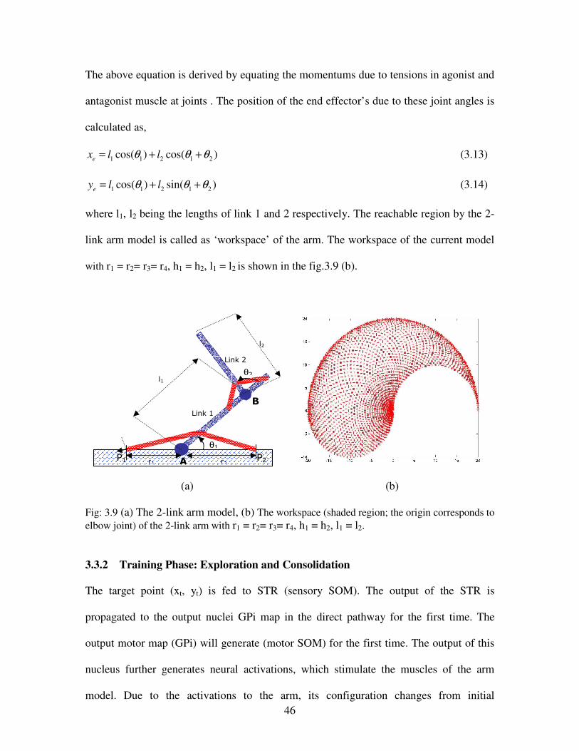
46
The above equation is derived by equating the momentums due to tensions in agonist and
antagonist muscle at joints . The position of the end effector’s due to these joint angles is
calculated as,
1 1 2 1 2cos( ) cos( )e
x l lθ θ θ= + + (3.13)
1 1 2 1 2cos( ) sin( )e
y l lθ θ θ= + + (3.14)
where l1, l2 being the lengths of link 1 and 2 respectively. The reachable region by the 2-
link arm model is called as ‘workspace’ of the arm. The workspace of the current model
with r1 = r2= r3= r4, h1 = h2, l1 = l2 is shown in the fig.3.9 (b).
(a) (b)
Fig: 3.9 (a) The 2-link arm model, (b) The workspace (shaded region; the origin corresponds to
elbow joint) of the 2-link arm with r1 = r2= r3= r4, h1 = h2, l1 = l2.
3.3.2 Training Phase: Exploration and Consolidation
The target point (xt, yt) is fed to STR (sensory SOM). The output of the STR is
propagated to the output nuclei GPi map in the direct pathway for the first time. The
output motor map (GPi) will generate (motor SOM) for the first time. The output of this
nucleus further generates neural activations, which stimulate the muscles of the arm
model. Due to the activations to the arm, its configuration changes from initial
θ1
Link 1
P1 P2 r1 r2 A
l1
Link 2
B
l2
θ2
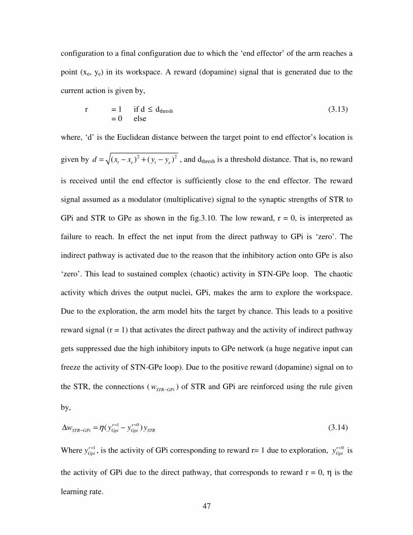
47
configuration to a final configuration due to which the ‘end effector’ of the arm reaches a
point (xe, ye) in its workspace. A reward (dopamine) signal that is generated due to the
current action is given by,
r = 1 if d ≤ dthresh (3.13)
= 0 else
where, ‘d’ is the Euclidean distance between the target point to end effector’s location is
given by 2 2( ) ( )t e t ed x x y y= − + − , and dthresh is a threshold distance. That is, no reward
is received until the end effector is sufficiently close to the end effector. The reward
signal assumed as a modulator (multiplicative) signal to the synaptic strengths of STR to
GPi and STR to GPe as shown in the fig.3.10. The low reward, r = 0, is interpreted as
failure to reach. In effect the net input from the direct pathway to GPi is ‘zero’. The
indirect pathway is activated due to the reason that the inhibitory action onto GPe is also
‘zero’. This lead to sustained complex (chaotic) activity in STN-GPe loop. The chaotic
activity which drives the output nuclei, GPi, makes the arm to explore the workspace.
Due to the exploration, the arm model hits the target by chance. This leads to a positive
reward signal (r = 1) that activates the direct pathway and the activity of indirect pathway
gets suppressed due the high inhibitory inputs to GPe network (a huge negative input can
freeze the activity of STN-GPe loop). Due to the positive reward (dopamine) signal on to
the STR, the connections (STR GPi
w − ) of STR and GPi are reinforced using the rule given
by,
1 0( )r r
STR GPi Gpi Gpi STRw y y yη = =−∆ = − (3.14)
Where 1r
Gpiy= , is the activity of GPi corresponding to reward r= 1 due to exploration, 0r
Gpiy= is
the activity of GPi due to the direct pathway, that corresponds to reward r = 0, η is the
learning rate.
48
Interpretation of pathways in BG as ‘consolidation’ and ‘exploration’ pathways
Fig.3.10. Microcircuit illustrating selection of pathways based on dopamine signal
The proposed model is a neural network architecture consisting of two parallel pathways
(fig.3.10). The pathways in BG, traditionally called “direct” and “indirect” pathways, can
be renamed as “consolidation” and “exploration” pathways based on their functional
roles. The consolidation pathway from STR to GPi consists of learnable connections that
represent the sensory-motor map involved in reaching task. The exploratory pathway
consisting of the STN-GPe loop is a network of oscillatory neurons; internal connections
among the oscillators are designed such that the STN-GPe loop produces chaotic activity
(similar to the model of STN-GPe in [13]). Output of the STN – GPe loop to GPi
provides a “noisy” or exploratory signal that is necessary for the realization of reward.
The reward signal, representing dopamine, from SNc is fed to STR which selects
between the consolidation pathway and the exploratory pathway depending on the reward
level. When the reward is low, the exploratory pathway is selected. Complex activity of
dthresh
d
-
GPi
STR
STN
GPe
gb ga
Indirect Direct
1/0 LEGEND
Inhibitory
Excitatory
Excitatory
Excitatory
Target
End effector
xt yt
SNc
49
STN-GPe loop, then, explores the output space, resulting in exploratory movement of the
arm. When the exploring arm chances upon the target, the system receives a strong
reward signal, the consolidation pathway is selected (the exploratory drive is suppressed)
and the connections between STR and GPi are reinforced in a Hebb-like fashion.
3.4 SUMMARY
In the current chapter, a computational model of BG is presented. The
computational model explains how BG can act as a source of exploratory drive.
Particularly an answer to the question of the functional significance of complex activity
in STN-GPe loop is suggested. It is also hypothesized that dopamine signal selects the
direct pathway and indirect pathway which act as consolidation and exploration
pathways, depending on the action generated. The training and testing results are
discussed in chapter 5.
In the previous chapter the functional significance of BG is presented highlighting
a point that it is involved in timing. Whereas in the present chapter it is shown that BG
has a role in exploratory drive. The next chapter deals with an integrated model of
handwriting generation and BG model. The dopamine deficient conditions in BG are
simulated to understand the Parkinsonian handwriting.
50
CHAPTER 4
UNDERSTANDING PARKINSONIAN HANDWRITING
THROUGH A COMPUTATIONAL MODEL
4.1 INTRODUCTION
Handwriting (HW) is a learned, highly practiced human motor skill that involves the
control and coordination of complex movement sequences. In the past decade,
handwriting has been gaining attention as a source of diagnostic information, in a variety
of neurological disorders including PD, Schizophrenia, and Obsessive Compulsive
Disorder (OCD) etc. Since handwriting, unlike reaching or walking, is a high-level
motor activity, it engages large parts of cortical and subcortical regions that include
SMA, PM, M1, BG, Cerebellum, Spinal cord etc. Since each of these regions contributes
to handwriting output in its own unique fashion, pathology of any of these regions is
manifest as characteristic features in handwriting. For example, in PD, a disorder of BG,
handwriting is marked by diminutive letter size or micrographia (van Gemmert et al,
1999; Teulings et al, 2002) (fig.1.a). Similarly handwriting in patients with cerebellar
damage is often characterized by omissions and unnecessary repetition of strokes
(fig.1.b) (Silvery et al, 1999). Recognition of rich diagnostic value of handwriting had
prompted a systematic study of handwriting and the extensive neuromotor organization
that generates it. Computational modeling offers an integrative framework in which
results of such studies – which come from several domains, like behavioral, imaging, etc
– are brought together and given a concrete shape.
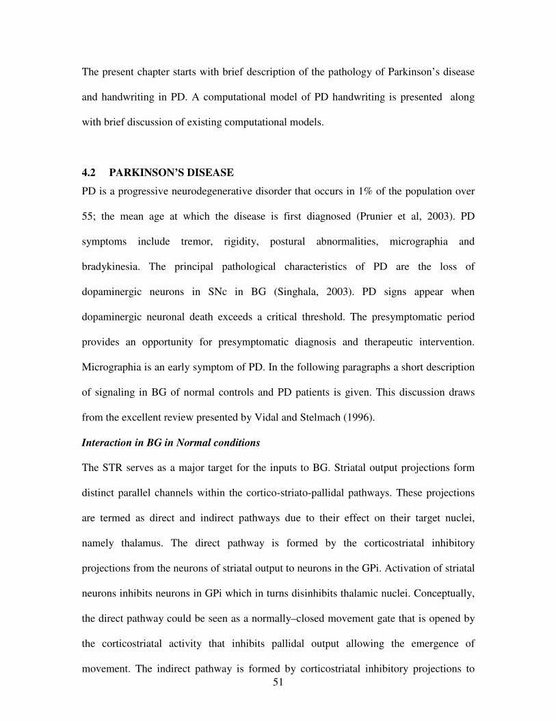
51
The present chapter starts with brief description of the pathology of Parkinson’s disease
and handwriting in PD. A computational model of PD handwriting is presented along
with brief discussion of existing computational models.
4.2 PARKINSON’S DISEASE
PD is a progressive neurodegenerative disorder that occurs in 1% of the population over
55; the mean age at which the disease is first diagnosed (Prunier et al, 2003). PD
symptoms include tremor, rigidity, postural abnormalities, micrographia and
bradykinesia. The principal pathological characteristics of PD are the loss of
dopaminergic neurons in SNc in BG (Singhala, 2003). PD signs appear when
dopaminergic neuronal death exceeds a critical threshold. The presymptomatic period
provides an opportunity for presymptomatic diagnosis and therapeutic intervention.
Micrographia is an early symptom of PD. In the following paragraphs a short description
of signaling in BG of normal controls and PD patients is given. This discussion draws
from the excellent review presented by Vidal and Stelmach (1996).
Interaction in BG in Normal conditions
The STR serves as a major target for the inputs to BG. Striatal output projections form
distinct parallel channels within the cortico-striato-pallidal pathways. These projections
are termed as direct and indirect pathways due to their effect on their target nuclei,
namely thalamus. The direct pathway is formed by the corticostriatal inhibitory
projections from the neurons of striatal output to neurons in the GPi. Activation of striatal
neurons inhibits neurons in GPi which in turns disinhibits thalamic nuclei. Conceptually,
the direct pathway could be seen as a normally–closed movement gate that is opened by
the corticostriatal activity that inhibits pallidal output allowing the emergence of
movement. The indirect pathway is formed by corticostriatal inhibitory projections to
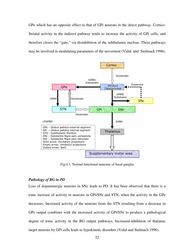
52
GPe which has an opposite effect to that of GPi neurons in the direct pathway. Cortico-
Striatal activity in the indirect pathway tends to increase the activity of GPi cells, and
therefore closes the “gate,” via disinhibition of the subthalamic nucleus. These pathways
may be involved in modulating parameters of the movement (Vidal and Stelmach 1996).
Fig.4.1. Normal functional anatomy of basal ganglia
Pathology of BG in PD
Loss of dopaminergic neurons in SNc leads to PD. It has been observed that there is a
tonic increase of activity in neurons in GPi/SNr and STN, when the activity in the GPe
decreases. Increased activity of the neurons from the STN resulting from a decrease in
GPe output combines with the increased activity of GPi/SNr to produce a pathological
degree of tonic activity in the BG output pathways. Increased-inhibition of thalamic
target neurons by GPi cells leads to hypokinetic disorders (Vidal and Stelmach 1996).
Cortex
GPe Striatum
(Acetylcholine
GABA
Glutamate
Glutamate GABA
GABA/ Enkephalin
Dopamine
Glutamate
GABA/ Substance
GPi SNr
Thalamus
Supplementary motor area
SNc
STN
GPe – Globus pallidus external segment GPi – Globus pallidus internal segment STN – Subthalamic Nucleus SNc – Substantia Nigra pars compancta SNr – Substantia Nigra pars reticulate Solid arrow: Excitatory projections Empty arrow: Inhibitory projections Dotted arrow: Both
LEGEND
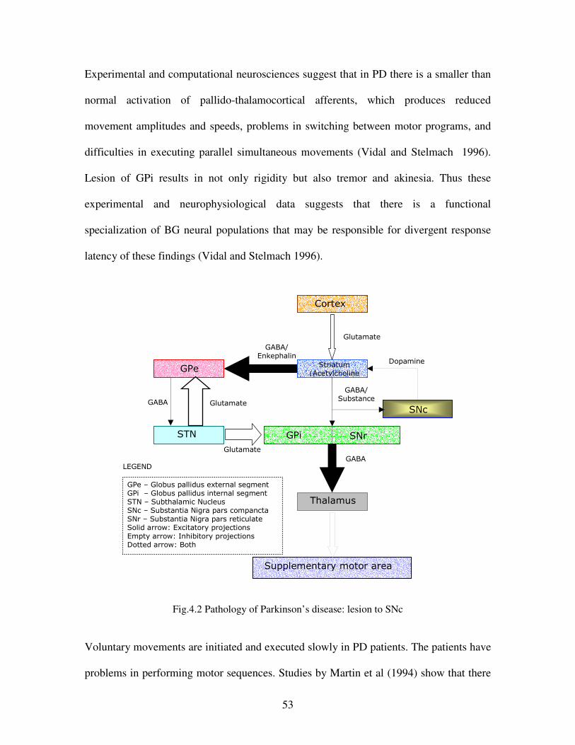
53
Experimental and computational neurosciences suggest that in PD there is a smaller than
normal activation of pallido-thalamocortical afferents, which produces reduced
movement amplitudes and speeds, problems in switching between motor programs, and
difficulties in executing parallel simultaneous movements (Vidal and Stelmach 1996).
Lesion of GPi results in not only rigidity but also tremor and akinesia. Thus these
experimental and neurophysiological data suggests that there is a functional
specialization of BG neural populations that may be responsible for divergent response
latency of these findings (Vidal and Stelmach 1996).
Fig.4.2 Pathology of Parkinson’s disease: lesion to SNc
Voluntary movements are initiated and executed slowly in PD patients. The patients have
problems in performing motor sequences. Studies by Martin et al (1994) show that there
Cortex
GPe Striatum
(Acetylcholine
Glutamate
Glutamate GABA
GABA/ Enkephalin
Dopamine
Glutamate
GABA/ Substance
GPi SNr
Thalamus
Supplementary motor area
SNc
STN
GABA LEGEND
GPe – Globus pallidus external segment GPi – Globus pallidus internal segment STN – Subthalamic Nucleus SNc – Substantia Nigra pars compancta SNr – Substantia Nigra pars reticulate Solid arrow: Excitatory projections Empty arrow: Inhibitory projections Dotted arrow: Both
54
exists instability in the movement sequence which is associated with irregular force
profile, increase in peak movement velocity, and target overshoot; the overshoot became
additive as the sequence was developed. It was also suggested that the tendency to slow
down may be favored by complex sequences such as handwriting and speech or tapping
(Vidal and Stelmach, 1996).
4.3 HANDWRITING IN PARKINSON’S DISEASE AND NEED FOR A
COMPUTATIONAL MODEL
HW in PD has a characteristically distorted form known as micrographia, marked by an
overall decrease in handwriting size, diminished legibility, and decreased movement
speed. Handwriting acquired from PD patients has been used for early diagnosis of the
PD also for the assessment of Drug-Induced PD (Guttman et al, 2003). There have been
attempts to estimate the stage of maturity of PD from analysis of HW (Cubbah and
Fairhrust, 2000, Stein, 2001). Such estimates have been used to control the dosage. They
provide a quantitative basis to taper dose during recovery. However, most of such
attempts to use HW for estimating disease stage are purely empirical, treating the brain as
a black-box; they do not originate in a precise functional understanding of BG. A
quantitative estimate of the stage of the disease is provided from the measured
handwriting features. However, most of such studies are of empirical nature. PD
handwriting is compared with that of normal subjects and the degree of difference is
quantified (Cubbah and Fairhrust, 2000). It would be desirable for such studies to be
backed up by a computational model that can explain why impairment in certain motor
modules should result in specific handwriting changes. Such a model will require a more
accurate understanding of the functional architecture of motor system.
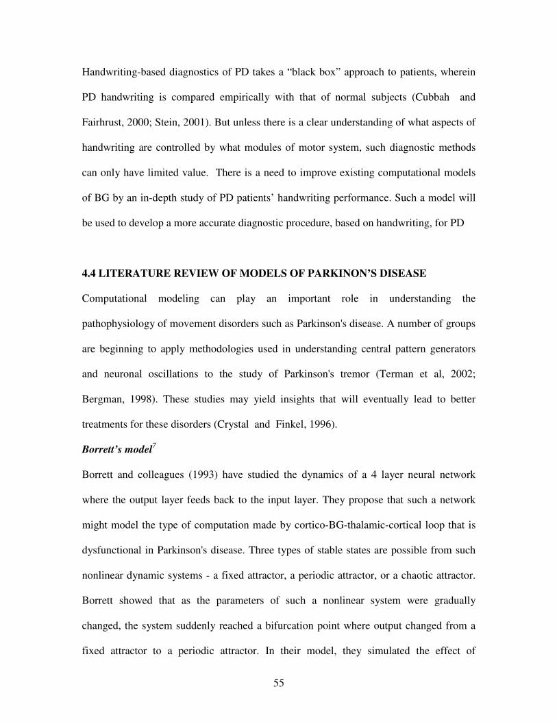
55
Handwriting-based diagnostics of PD takes a “black box” approach to patients, wherein
PD handwriting is compared empirically with that of normal subjects (Cubbah and
Fairhrust, 2000; Stein, 2001). But unless there is a clear understanding of what aspects of
handwriting are controlled by what modules of motor system, such diagnostic methods
can only have limited value. There is a need to improve existing computational models
of BG by an in-depth study of PD patients’ handwriting performance. Such a model will
be used to develop a more accurate diagnostic procedure, based on handwriting, for PD
4.4 LITERATURE REVIEW OF MODELS OF PARKINON’S DISEASE
Computational modeling can play an important role in understanding the
pathophysiology of movement disorders such as Parkinson's disease. A number of groups
are beginning to apply methodologies used in understanding central pattern generators
and neuronal oscillations to the study of Parkinson's tremor (Terman et al, 2002;
Bergman, 1998). These studies may yield insights that will eventually lead to better
treatments for these disorders (Crystal and Finkel, 1996).
Borrett’s model7
Borrett and colleagues (1993) have studied the dynamics of a 4 layer neural network
where the output layer feeds back to the input layer. They propose that such a network
might model the type of computation made by cortico-BG-thalamic-cortical loop that is
dysfunctional in Parkinson's disease. Three types of stable states are possible from such
nonlinear dynamic systems - a fixed attractor, a periodic attractor, or a chaotic attractor.
Borrett showed that as the parameters of such a nonlinear system were gradually
changed, the system suddenly reached a bifurcation point where output changed from a
fixed attractor to a periodic attractor. In their model, they simulated the effect of
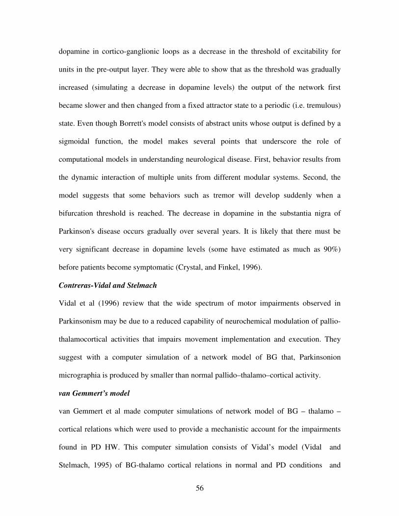
56
dopamine in cortico-ganglionic loops as a decrease in the threshold of excitability for
units in the pre-output layer. They were able to show that as the threshold was gradually
increased (simulating a decrease in dopamine levels) the output of the network first
became slower and then changed from a fixed attractor state to a periodic (i.e. tremulous)
state. Even though Borrett's model consists of abstract units whose output is defined by a
sigmoidal function, the model makes several points that underscore the role of
computational models in understanding neurological disease. First, behavior results from
the dynamic interaction of multiple units from different modular systems. Second, the
model suggests that some behaviors such as tremor will develop suddenly when a
bifurcation threshold is reached. The decrease in dopamine in the substantia nigra of
Parkinson's disease occurs gradually over several years. It is likely that there must be
very significant decrease in dopamine levels (some have estimated as much as 90%)
before patients become symptomatic (Crystal, and Finkel, 1996).
Contreras-Vidal and Stelmach
Vidal et al (1996) review that the wide spectrum of motor impairments observed in
Parkinsonism may be due to a reduced capability of neurochemical modulation of pallio-
thalamocortical activities that impairs movement implementation and execution. They
suggest with a computer simulation of a network model of BG that, Parkinsonion
micrographia is produced by smaller than normal pallido–thalamo–cortical activity.
van Gemmert’s model
van Gemmert et al made computer simulations of network model of BG – thalamo –
cortical relations which were used to provide a mechanistic account for the impairments
found in PD HW. This computer simulation consists of Vidal’s model (Vidal and
Stelmach, 1995) of BG-thalamo cortical relations in normal and PD conditions and
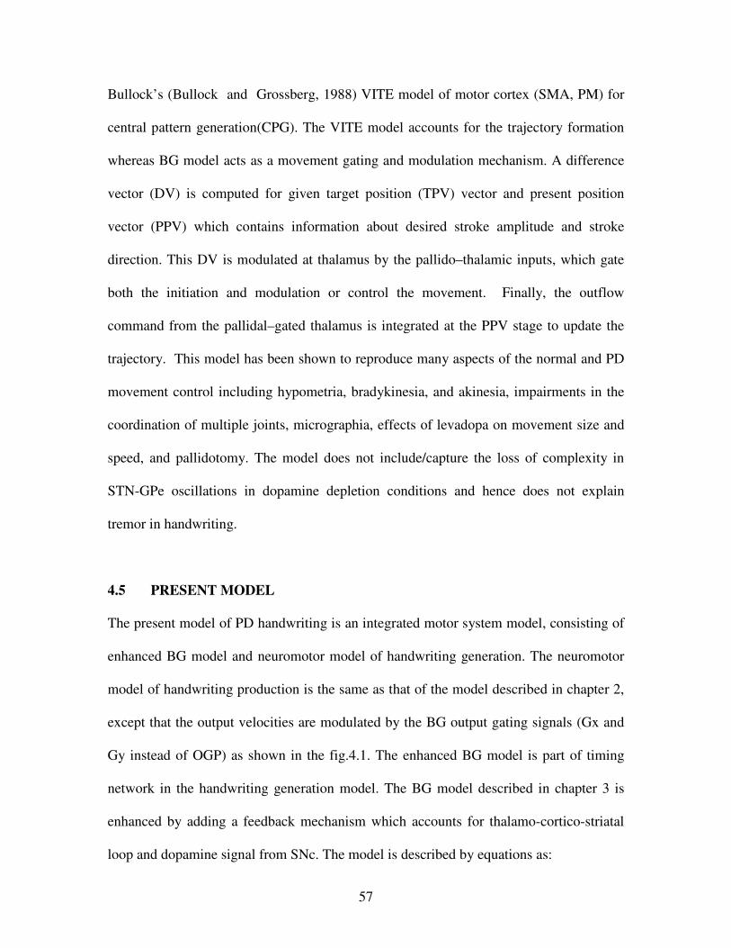
57
Bullock’s (Bullock and Grossberg, 1988) VITE model of motor cortex (SMA, PM) for
central pattern generation(CPG). The VITE model accounts for the trajectory formation
whereas BG model acts as a movement gating and modulation mechanism. A difference
vector (DV) is computed for given target position (TPV) vector and present position
vector (PPV) which contains information about desired stroke amplitude and stroke
direction. This DV is modulated at thalamus by the pallido–thalamic inputs, which gate
both the initiation and modulation or control the movement. Finally, the outflow
command from the pallidal–gated thalamus is integrated at the PPV stage to update the
trajectory. This model has been shown to reproduce many aspects of the normal and PD
movement control including hypometria, bradykinesia, and akinesia, impairments in the
coordination of multiple joints, micrographia, effects of levadopa on movement size and
speed, and pallidotomy. The model does not include/capture the loss of complexity in
STN-GPe oscillations in dopamine depletion conditions and hence does not explain
tremor in handwriting.
4.5 PRESENT MODEL
The present model of PD handwriting is an integrated motor system model, consisting of
enhanced BG model and neuromotor model of handwriting generation. The neuromotor
model of handwriting production is the same as that of the model described in chapter 2,
except that the output velocities are modulated by the BG output gating signals (Gx and
Gy instead of OGP) as shown in the fig.4.1. The enhanced BG model is part of timing
network in the handwriting generation model. The BG model described in chapter 3 is
enhanced by adding a feedback mechanism which accounts for thalamo-cortico-striatal
loop and dopamine signal from SNc. The model is described by equations as:
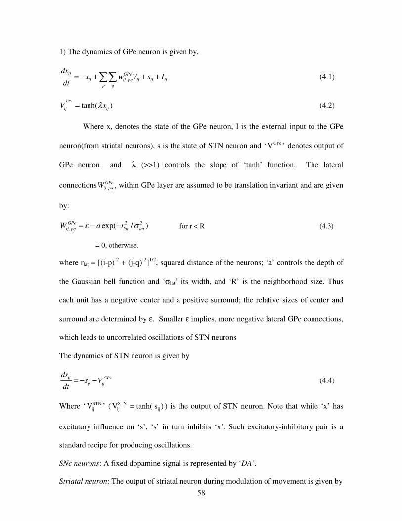
58
1) The dynamics of GPe neuron is given by,
,
ij GPe
ij ij pq ij ij ij
p q
dxx w V s I
dt= − + + +∑∑ (4.1)
tanh( )GPe
ij ijV xλ= (4.2)
Where x, denotes the state of the GPe neuron, I is the external input to the GPe
neuron(from striatal neurons), s is the state of STN neuron and ‘ GPeV ’ denotes output of
GPe neuron and λ (>>1) controls the slope of ‘tanh’ function. The lateral
connections ,
GPe
ij pqW , within GPe layer are assumed to be translation invariant and are given
by:
2 2
, exp( / )GPe
ij pq lat latW a rε σ= − − for r < R (4.3)
= 0, otherwise.
where rlat = [(i-p) 2
+ (j-q) 2
]1/2
, squared distance of the neurons; ‘a’ controls the depth of
the Gaussian bell function and ‘σlat’ its width, and ‘R’ is the neighborhood size. Thus
each unit has a negative center and a positive surround; the relative sizes of center and
surround are determined by ε. Smaller ε implies, more negative lateral GPe connections,
which leads to uncorrelated oscillations of STN neurons
The dynamics of STN neuron is given by
ij GPe
ij ij
dss V
dt= − − (4.4)
Where ‘ STN
ijV ’ ( STN
ij ijV = tanh( s ) ) is the output of STN neuron. Note that while ‘x’ has
excitatory influence on ‘s’, ‘s’ in turn inhibits ‘x’. Such excitatory-inhibitory pair is a
standard recipe for producing oscillations.
SNc neurons: A fixed dopamine signal is represented by ‘DA’.
Striatal neuron: The output of striatal neuron during modulation of movement is given by
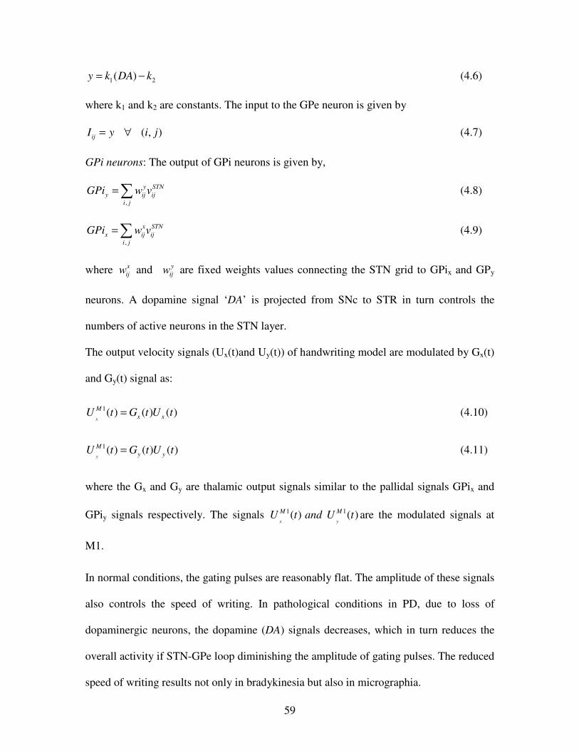
59
1 2( )y k DA k= − (4.6)
where k1 and k2 are constants. The input to the GPe neuron is given by
( , )ij
I y i j= ∀ (4.7)
GPi neurons: The output of GPi neurons is given by,
,
y STN
y ij ij
i j
GPi w v=∑ (4.8)
,
x STN
x ij ij
i j
GPi w v=∑ (4.9)
where x
ijw and y
ijw are fixed weights values connecting the STN grid to GPix and GPy
neurons. A dopamine signal ‘DA’ is projected from SNc to STR in turn controls the
numbers of active neurons in the STN layer.
The output velocity signals (Ux(t)and Uy(t)) of handwriting model are modulated by Gx(t)
and Gy(t) signal as:
1( ) ( ) ( )x
M
x xU t G t U t= (4.10)
1( ) ( ) ( )y
M
y yU t G t U t= (4.11)
where the Gx and Gy are thalamic output signals similar to the pallidal signals GPix and
GPiy signals respectively. The signals 1 1( ) ( )x y
M MU t and U t are the modulated signals at
M1.
In normal conditions, the gating pulses are reasonably flat. The amplitude of these signals
also controls the speed of writing. In pathological conditions in PD, due to loss of
dopaminergic neurons, the dopamine (DA) signals decreases, which in turn reduces the
overall activity if STN-GPe loop diminishing the amplitude of gating pulses. The reduced
speed of writing results not only in bradykinesia but also in micrographia.
60
Fig.4.3: Integrated neuromotor model of handwriting generation
Fig. 4.4. Mapping the integrated model on to neuroanatomy
The STN – GPe neurons are connected in excitatory and inhibitory fashion: such
connectivity is known to produce a range of dynamic behaviors like clustering, traveling
waves and chaos (Terman, 2002) as discussed in chapter 3. It can be observed that for
desired flat profile of gating signals the network needs to be in chaotic mode. Lesions can
be introduced also into STN-GPe activity by disrupting the connection strengths of GPe
loop. These lesions in STN-GPe loop will reduce the complexity of interaction that
INPUT ξ
TIMING
NETWORK
X(t) Y(t)
Ux(t) Uy(t) OGP
PP
OGP STN - GPe
Dopamine
- -
GPi
Gx Gy
Striatum
GPi
STR
SNc
Thalamus
GPe
preSMA / PM
SMA
Spinal cord
Cortex
STN
DA
Gx and Gy
PP
GP
BASAL GANGLIA NEUROMOTOR MODEL
Ux and Uy
Basal Ganglia
GPix and GPiy
61
results in traveling wave activity of STN producing wavy handwriting. These results are
explained in detail in chapter 5.
4.6 SUMMARY
In the present chapter, the pathology of PD and handwriting in PD were discussed. Need
for a computational model for understanding handwriting in PD is discussed. And a
computational model of PD handwriting is presented. The results of this model are
discussed in detail in chapter 5. Conclusions and predictions are discussed in chapter 6.
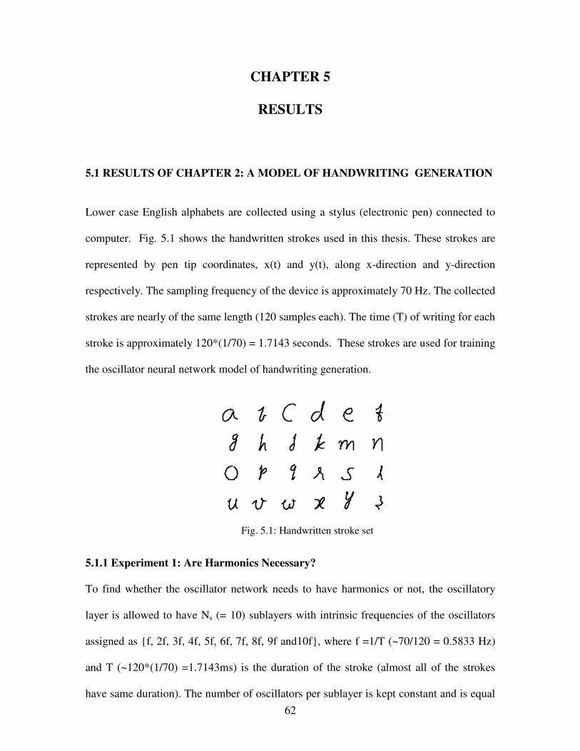
62
CHAPTER 5
RESULTS
5.1 RESULTS OF CHAPTER 2: A MODEL OF HANDWRITING GENERATION
Lower case English alphabets are collected using a stylus (electronic pen) connected to
computer. Fig. 5.1 shows the handwritten strokes used in this thesis. These strokes are
represented by pen tip coordinates, x(t) and y(t), along x-direction and y-direction
respectively. The sampling frequency of the device is approximately 70 Hz. The collected
strokes are nearly of the same length (120 samples each). The time (T) of writing for each
stroke is approximately 120*(1/70) = 1.7143 seconds. These strokes are used for training
the oscillator neural network model of handwriting generation.
Fig. 5.1: Handwritten stroke set
5.1.1 Experiment 1: Are Harmonics Necessary?
To find whether the oscillator network needs to have harmonics or not, the oscillatory
layer is allowed to have Ns (= 10) sublayers with intrinsic frequencies of the oscillators
assigned as {f, 2f, 3f, 4f, 5f, 6f, 7f, 8f, 9f and10f}, where f =1/T (~70/120 = 0.5833 Hz)
and T (~120*(1/70) =1.7143ms) is the duration of the stroke (almost all of the strokes
have same duration). The number of oscillators per sublayer is kept constant and is equal
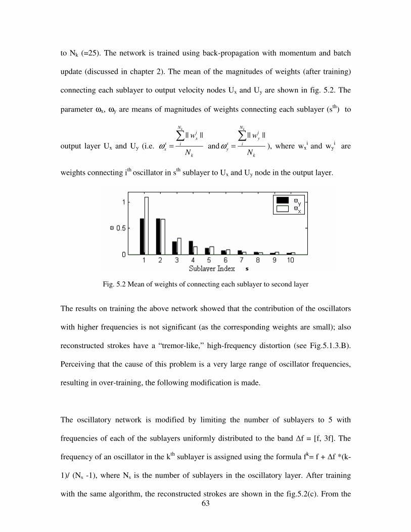
63
to Nk (=25). The network is trained using back-propagation with momentum and batch
update (discussed in chapter 2). The mean of the magnitudes of weights (after training)
connecting each sublayer to output velocity nodes Ux and Uy are shown in fig. 5.2. The
parameter ωx, ωy are means of magnitudes of weights connecting each sublayer (sth
) to
output layer Ux and Uy (i.e.
|| ||kN
i
xs ix
k
w
Nω =
∑ and
|| ||kN
i
ys iy
k
w
Nω =
∑), where wx
i and wy
i are
weights connecting ith
oscillator in sth
sublayer to Ux and Uy node in the output layer.
Fig. 5.2 Mean of weights of connecting each sublayer to second layer
The results on training the above network showed that the contribution of the oscillators
with higher frequencies is not significant (as the corresponding weights are small); also
reconstructed strokes have a “tremor-like,” high-frequency distortion (see Fig.5.1.3.B).
Perceiving that the cause of this problem is a very large range of oscillator frequencies,
resulting in over-training, the following modification is made.
The oscillatory network is modified by limiting the number of sublayers to 5 with
frequencies of each of the sublayers uniformly distributed to the band ∆f = [f, 3f]. The
frequency of an oscillator in the kth
sublayer is assigned using the formula fk= f + ∆f *(k-
1)/ (Ns -1), where Ns is the number of sublayers in the oscillatory layer. After training
with the same algorithm, the reconstructed strokes are shown in the fig.5.2(c). From the
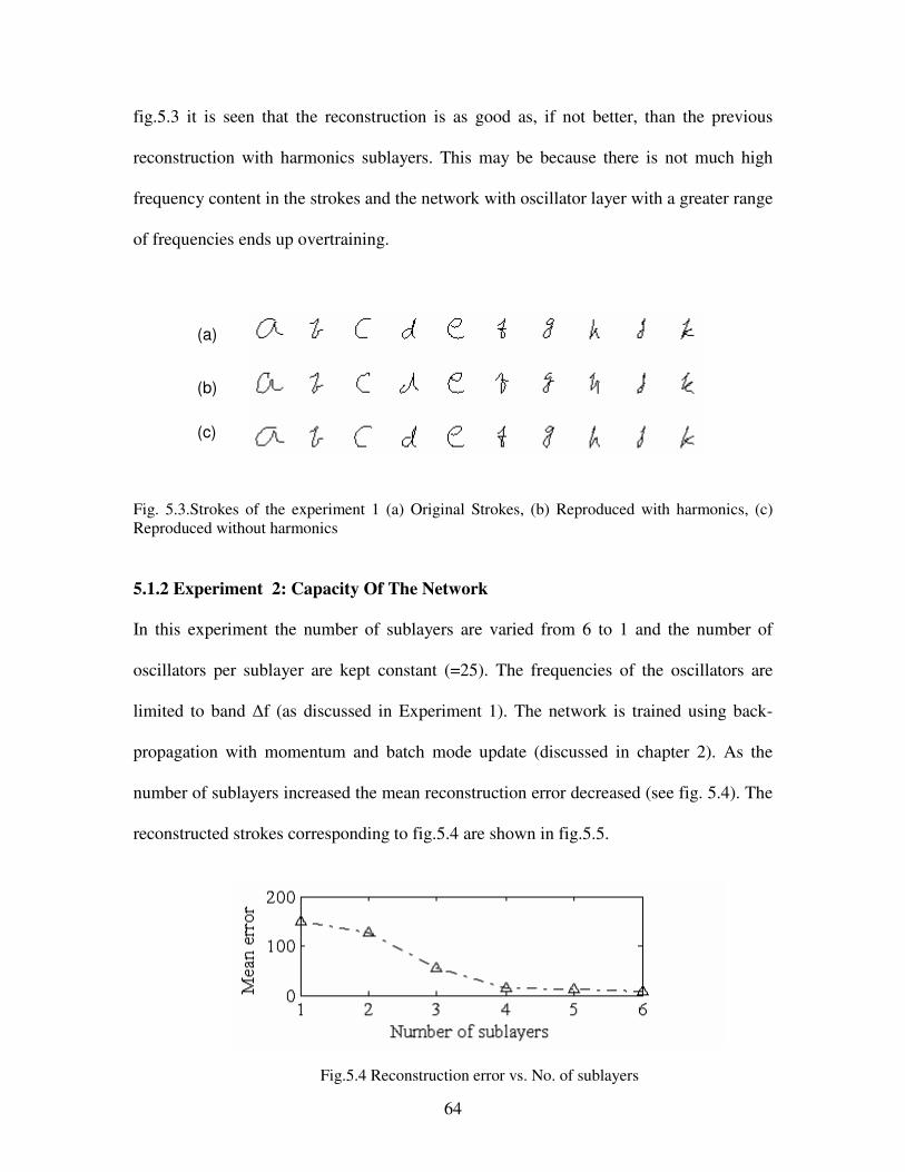
64
fig.5.3 it is seen that the reconstruction is as good as, if not better, than the previous
reconstruction with harmonics sublayers. This may be because there is not much high
frequency content in the strokes and the network with oscillator layer with a greater range
of frequencies ends up overtraining.
Fig. 5.3.Strokes of the experiment 1 (a) Original Strokes, (b) Reproduced with harmonics, (c)
Reproduced without harmonics
5.1.2 Experiment 2: Capacity Of The Network
In this experiment the number of sublayers are varied from 6 to 1 and the number of
oscillators per sublayer are kept constant (=25). The frequencies of the oscillators are
limited to band ∆f (as discussed in Experiment 1). The network is trained using back-
propagation with momentum and batch mode update (discussed in chapter 2). As the
number of sublayers increased the mean reconstruction error decreased (see fig. 5.4). The
reconstructed strokes corresponding to fig.5.4 are shown in fig.5.5.
Fig.5.4 Reconstruction error vs. No. of sublayers
(a)
(c)
(b)
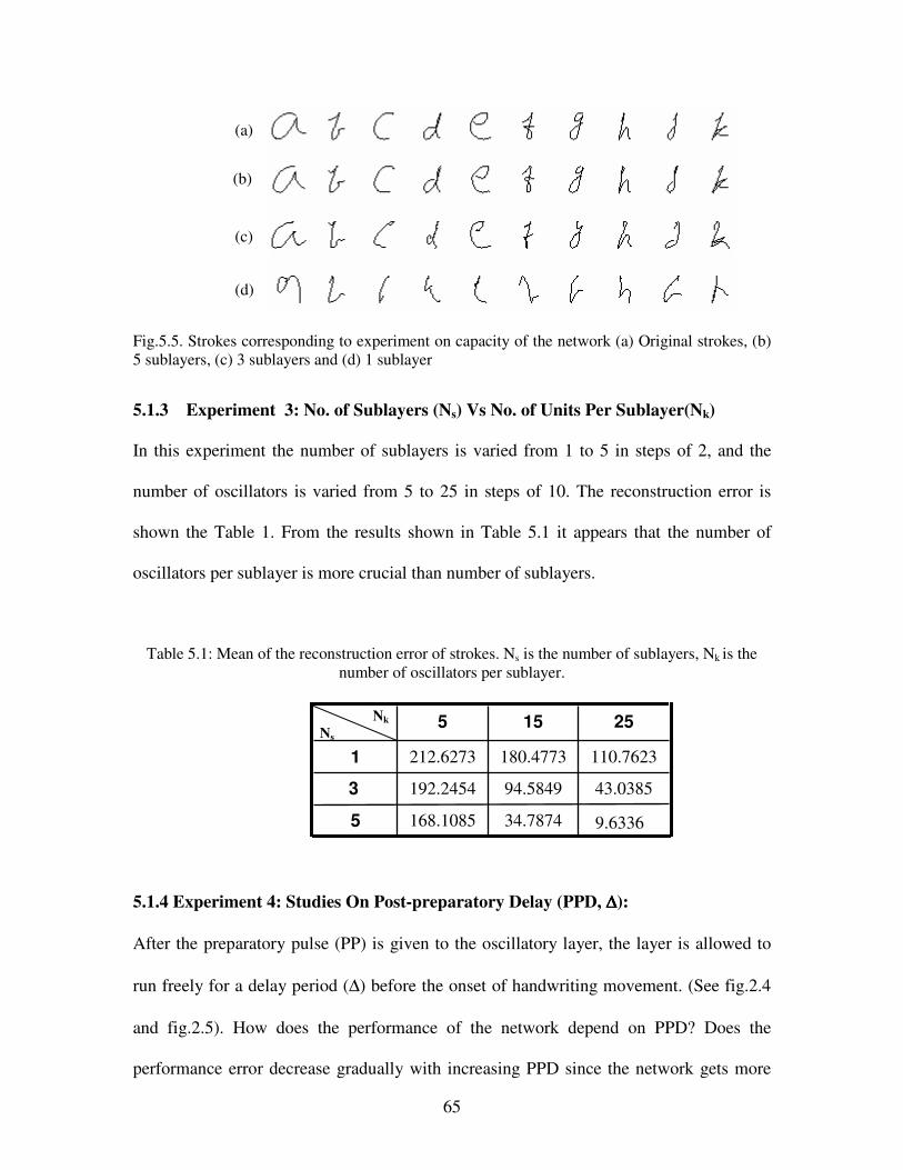
65
Fig.5.5. Strokes corresponding to experiment on capacity of the network (a) Original strokes, (b)
5 sublayers, (c) 3 sublayers and (d) 1 sublayer
5.1.3 Experiment 3: No. of Sublayers (Ns) Vs No. of Units Per Sublayer(Nk)
In this experiment the number of sublayers is varied from 1 to 5 in steps of 2, and the
number of oscillators is varied from 5 to 25 in steps of 10. The reconstruction error is
shown the Table 1. From the results shown in Table 5.1 it appears that the number of
oscillators per sublayer is more crucial than number of sublayers.
Table 5.1: Mean of the reconstruction error of strokes. Ns is the number of sublayers, Nk is the
number of oscillators per sublayer.
5.1.4 Experiment 4: Studies On Post-preparatory Delay (PPD, ∆∆∆∆):
After the preparatory pulse (PP) is given to the oscillatory layer, the layer is allowed to
run freely for a delay period (∆) before the onset of handwriting movement. (See fig.2.4
and fig.2.5). How does the performance of the network depend on PPD? Does the
performance error decrease gradually with increasing PPD since the network gets more
9.6336 34.7874 168.1085 5
43.0385 94.5849 192.2454 3
110.7623 180.4773 212.6273 1
25 15 5
(a)
(b)
(c)
(d)
Nk
Ns
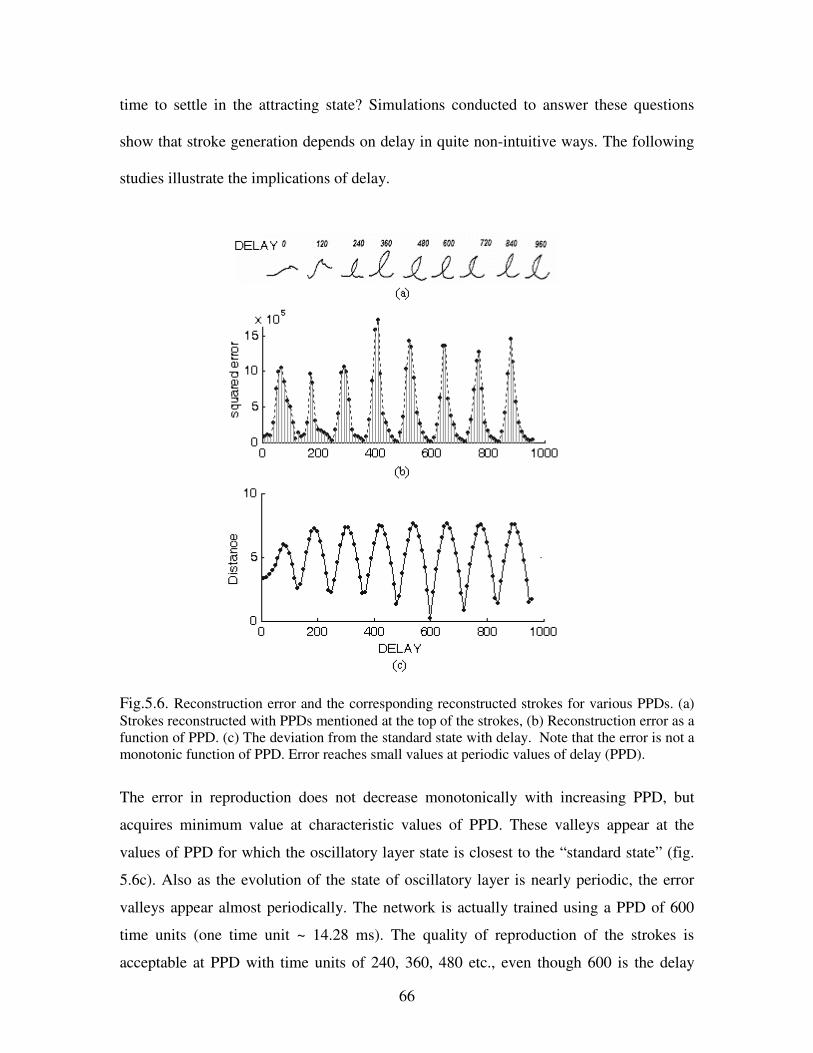
66
time to settle in the attracting state? Simulations conducted to answer these questions
show that stroke generation depends on delay in quite non-intuitive ways. The following
studies illustrate the implications of delay.
Fig.5.6. Reconstruction error and the corresponding reconstructed strokes for various PPDs. (a)
Strokes reconstructed with PPDs mentioned at the top of the strokes, (b) Reconstruction error as a
function of PPD. (c) The deviation from the standard state with delay. Note that the error is not a
monotonic function of PPD. Error reaches small values at periodic values of delay (PPD).
The error in reproduction does not decrease monotonically with increasing PPD, but
acquires minimum value at characteristic values of PPD. These valleys appear at the
values of PPD for which the oscillatory layer state is closest to the “standard state” (fig.
5.6c). Also as the evolution of the state of oscillatory layer is nearly periodic, the error
valleys appear almost periodically. The network is actually trained using a PPD of 600
time units (one time unit ~ 14.28 ms). The quality of reproduction of the strokes is
acceptable at PPD with time units of 240, 360, 480 etc., even though 600 is the delay
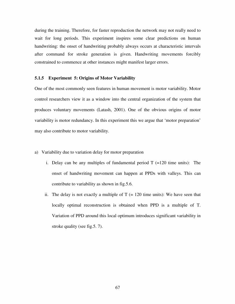
67
during the training. Therefore, for faster reproduction the network may not really need to
wait for long periods. This experiment inspires some clear predictions on human
handwriting: the onset of handwriting probably always occurs at characteristic intervals
after command for stroke generation is given. Handwriting movements forcibly
constrained to commence at other instances might manifest larger errors.
5.1.5 Experiment 5: Origins of Motor Variability
One of the most commonly seen features in human movement is motor variability. Motor
control researchers view it as a window into the central organization of the system that
produces voluntary movements (Latash, 2001). One of the obvious origins of motor
variability is motor redundancy. In this experiment this we argue that ‘motor preparation’
may also contribute to motor variability.
a) Variability due to variation delay for motor preparation
i. Delay can be any multiples of fundamental period T (=120 time units): The
onset of handwriting movement can happen at PPDs with valleys. This can
contribute to variability as shown in fig.5.6.
ii. The delay is not exactly a multiple of T (= 120 time units): We have seen that
locally optimal reconstruction is obtained when PPD is a multiple of T.
Variation of PPD around this local optimum introduces significant variability in
stroke quality (see fig.5. 7).
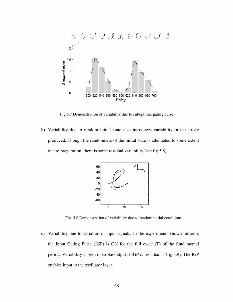
68
Fig.5.7 Demonstration of variability due to suboptimal gating pulse
b) Variability due to random initial state also introduces variability in the stroke
produced. Though the randomness of the initial state is attenuated to some extent
due to preparation, there is some residual variability (see fig.5.8).
Fig. 5.8 Demonstration of variability due to random initial conditions
c) Variability due to variation in input signals: In the experiments shown hitherto,
the Input Gating Pulse (IGP) is ON for the full cycle (T) of the fundamental
period. Variability is seen in stroke output if IGP is less than T (fig.5.9). The IGP
enables input to the oscillator layer.
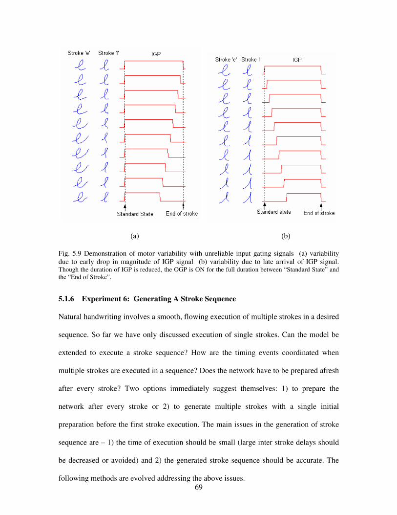
69
(a) (b)
Fig. 5.9 Demonstration of motor variability with unreliable input gating signals (a) variability
due to early drop in magnitude of IGP signal (b) variability due to late arrival of IGP signal. Though the duration of IGP is reduced, the OGP is ON for the full duration between “Standard State” and
the “End of Stroke”.
5.1.6 Experiment 6: Generating A Stroke Sequence
Natural handwriting involves a smooth, flowing execution of multiple strokes in a desired
sequence. So far we have only discussed execution of single strokes. Can the model be
extended to execute a stroke sequence? How are the timing events coordinated when
multiple strokes are executed in a sequence? Does the network have to be prepared afresh
after every stroke? Two options immediately suggest themselves: 1) to prepare the
network after every stroke or 2) to generate multiple strokes with a single initial
preparation before the first stroke execution. The main issues in the generation of stroke
sequence are – 1) the time of execution should be small (large inter stroke delays should
be decreased or avoided) and 2) the generated stroke sequence should be accurate. The
following methods are evolved addressing the above issues.
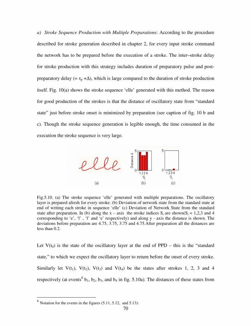
70
a) Stroke Sequence Production with Multiple Preparations: According to the procedure
described for stroke generation described in chapter 2, for every input stroke command
the network has to be prepared before the execution of a stroke. The inter–stroke delay
for stroke production with this strategy includes duration of preparatory pulse and post-
preparatory delay (= τp +∆), which is large compared to the duration of stroke production
itself. Fig. 10(a) shows the stroke sequence ‘elle’ generated with this method. The reason
for good production of the strokes is that the distance of oscillatory state from “standard
state” just before stroke onset is minimized by preparation (see caption of fig. 10 b and
c). Though the stroke sequence generation is legible enough, the time consumed in the
execution the stroke sequence is very large.
Fig.5.10. (a) The stroke sequence ‘elle’ generated with multiple preparations. The oscillatory
layer is prepared afresh for every stroke. (b) Deviation of network state from the standard state at
end of writing each stroke in sequence ‘elle’ (c) Deviation of Network State from the standard
state after preparation. In (b) along the x – axis the stroke indices Si are shown(Si = 1,2,3 and 4
corresponding to ‘e’, ‘l’ , ‘l’ and ‘e’ respectively) and along y - axis the distance is shown. The
deviations before preparation are 4.75, 3.75, 3.75 and 4.75.After preparation all the distances are
less than 0.2.
Let V(t0) is the state of the oscillatory layer at the end of PPD – this is the “standard
state,” to which we expect the oscillatory layer to return before the onset of every stroke.
Similarly let V(t1), V(t2), V(t3) and V(t4) be the states after strokes 1, 2, 3 and 4
respectively (at events8 b1, b2, b3, and b4 in fig. 5.10a). The distances of these states from
8 Notation for the events in the figures (5.11, 5.12, and 5.13):
71
standard state, V(t0) is shown in fig.5.10b. Note that this distance is shortened drastically
by the preparation. Due to the lesser deviation of state from the standard state, the quality
of the stroke sequence generation is superior. However, to allow a full preparatory delay
after every stroke makes execution too long. How can the delay in inter-stroke
preparation be minimized?
b) Stroke Sequence Production with Single Preparation and Full duration IGP:
In order to reduce the inordinately long time required to prepare the network after every
stroke, we now allow the network to execute the entire stroke sequence as shown in
fig.11c. The first two strokes ‘e’ and ‘l’ generated are legible but the subsequent strokes
are illegible (see fig.11a). The reason why stroke reconstruction is poor with single
preparation is that the state of oscillatory layer is disturbed after presentation of every
stroke command and does not return to the standard state before the next stroke begins
(see caption of fig. 11b). Poor reconstruction is only natural. One way to improve the
quality of the stroke sequence generation may be to allow the network to evolve freely,
without input, for sometime between strokes. Since the oscillatory layer evolves to its
limit cycle attractor in free-running (no input) condition, it might approach the “standard
state” sufficiently closely.
� P1, P2, P3 and P4 are start of preparatory pulses corresponding to strokes ‘e’, ‘l’, ‘l’ and ‘e’
respectively.
� a1, a2, a3 and a4 are start of input gate pulse (IGP) and start of output gate pulse (OGP) of the strokes
‘e’, ‘l’, ‘l’ and ‘e’ respectively.
� b1, b2, b3 and b4 are end of output gate pulse (OGP) of the strokes ‘e’, ‘l’, ‘l’ and ‘e’ respectively.
� c1, c2, c3 and c4 are end of input gate pulse (IGP) of the strokes ‘e’, ‘l’, ‘l’ and ‘e’ respectively.
72
Fig.5.11. Generation of stroke sequence ‘elle’ with single preparation and fixed full duration
input gate pulse (IGP). (a) The generated stroke sequence, (b) the distance of deviation from the
networks state at the end of each stroke to the standard state. (c) Illustration of events in the
production of stroke sequence ‘elle’ with preparatory and gating signals. The oscillator network
is prepared only at the arrival of first input stroke command. There is no preparation between
strokes. The strokes are executed in continuous fashion one after other without any delay. The
first two strokes seem to be legible, but the later ones are not. The execution time is reduced at
the cost of legibility of the stroke. The oscillatory layer state does not return to the “standard
state”. The distances of the states of oscillatory layer from the “standard state” just before the
stroke onset are 3.3, 4.9, 5.15, and 4.75 respectively.
c) Stroke Sequence Production with Single Preparation with Partial IGP:
In the previous method, the Input Gating Pulse (IGP) to a stroke comes ON just when the
IGP for the previous pulse turns OFF. That is, there is never a time when the oscillatory
layer receives no input; it is never in a free-running condition. Therefore, in this method,
for each input stroke, the IGP is reset to OFF state a little before (=30 time units) the
73
execution of the stroke finishes. That is, there is a free-running period of 30 time units
between consecutive strokes. The stroke sequence generated with this method is shown in
fig. 12a. Though reconstruction of strokes 3 and 4 in ‘elle’ is better than that of the
previous method, the distortion is still unacceptable. The distances of oscillatory layer
states from “standard state” is lesser than those of the previous case (see captions fig.11
and fig.12) but still unacceptably high. Is it possible to decrease them further? Reliable
stroke reconstruction seems to depend crucially on the choice of the instant of stroke
onset.
To fix this problem one must only look for a way of determining the exact instant when
the network comes closest to the standard state, even if not identical. On a careful
analysis of the evolution of the state of the oscillatory layer, V(t), it became clear that the
frequency of the state in the “free-running” intervals between strokes is not constant. For
example, in the simulation of fig.12, the period of oscillation of the first sublayer during
the preparatory period is 120 time units; corresponding values in the “free-running”
intervals between strokes 1 and 2, strokes 2 and 3, strokes 3 and 4 and after stroke 4 are
103 time units, 87 time units, 95 time units and 106 time units respectively9. The actual
frequency depends in a complex way on the exact command input presented. Since there
is a shift in frequency, and only a small one at that, there is no compelling reason for the
state of the oscillatory layer to return precisely to the standard state, V(t0). What then is
the appropriate moment to start a new stroke once a stroke is executed?
9These approximate values are calculated for the first period in the free running mode. However a deviation
of period is observed in the later periods.
74
Fig. 5.12.Generation of stroke sequence ‘elle’ with single preparation and partial duration input
gate pulse (IGP). (a) the generated stroke sequence, (b) the distance of deviation from the
networks state at the end of each stroke to the standard state. (c) The events during the generation
of the stroke sequence ‘elle’. The oscillator network is prepared only before the first stroke. There
is no preparation between strokes. But the IGP for a given stroke is not ON throughout the stroke
execution period, T. For example, IGP of stroke 1 is turned OFF at ‘c1’ and IGP of stroke 2 is
turned ON only at ‘a2’. Though the strokes generated with this method are more legible that that
of previous method, the legibility of the stroke generated is not appreciable. The distances of the
oscillatory layer state from the “standard state” in this case are 2.7, 2.9, 3.4, and 4.5 respectively.
d) Stroke Sequence Production with Phase-triggered IGP:
The solution to the above predicament lies in the observation that accurate generation of a
learnt stroke depends not necessarily on preparing the network to reach the standard
amplitude state, V(t0)), but only to a standard phase state, φ(t0). Though the frequency is
slightly altered in the “free-running” period between strokes, it is obvious that the phase
relationships among oscillators of the oscillatory layer are still preserved and the layer
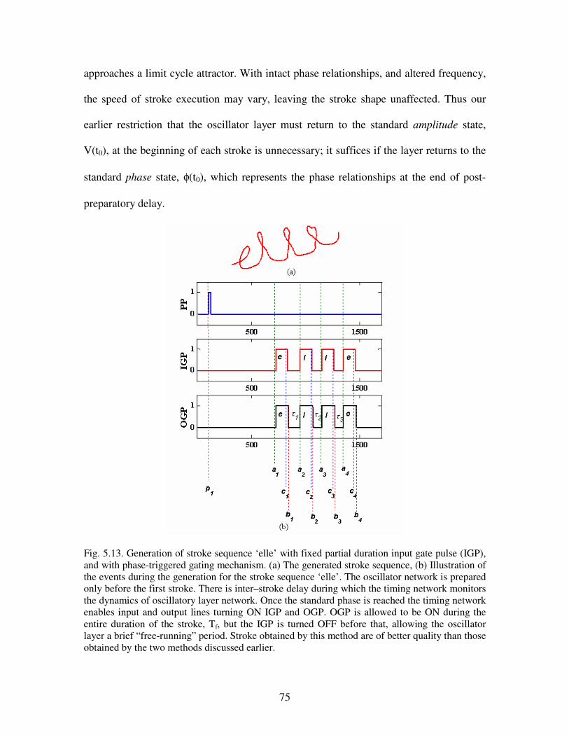
75
approaches a limit cycle attractor. With intact phase relationships, and altered frequency,
the speed of stroke execution may vary, leaving the stroke shape unaffected. Thus our
earlier restriction that the oscillator layer must return to the standard amplitude state,
V(t0), at the beginning of each stroke is unnecessary; it suffices if the layer returns to the
standard phase state, φ(t0), which represents the phase relationships at the end of post-
preparatory delay.
Fig. 5.13. Generation of stroke sequence ‘elle’ with fixed partial duration input gate pulse (IGP),
and with phase-triggered gating mechanism. (a) The generated stroke sequence, (b) Illustration of
the events during the generation for the stroke sequence ‘elle’. The oscillator network is prepared
only before the first stroke. There is inter–stroke delay during which the timing network monitors
the dynamics of oscillatory layer network. Once the standard phase is reached the timing network
enables input and output lines turning ON IGP and OGP. OGP is allowed to be ON during the
entire duration of the stroke, Tf, but the IGP is turned OFF before that, allowing the oscillator
layer a brief “free-running” period. Stroke obtained by this method are of better quality than those
obtained by the two methods discussed earlier.
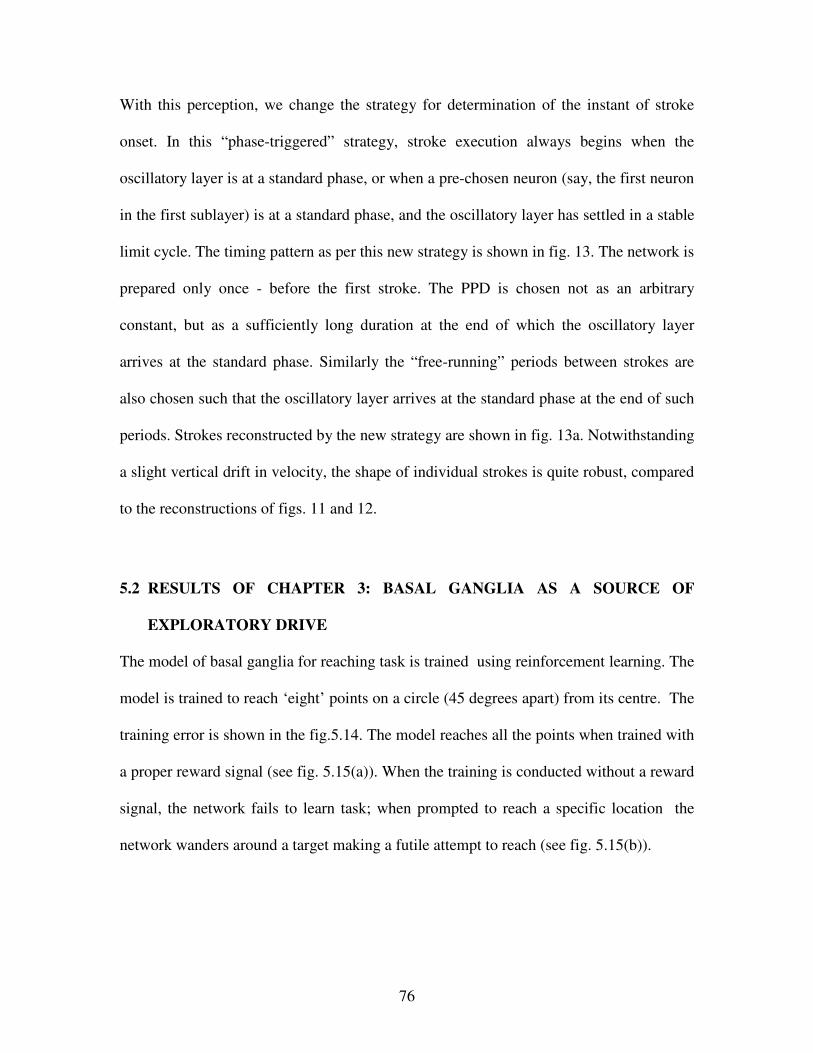
76
With this perception, we change the strategy for determination of the instant of stroke
onset. In this “phase-triggered” strategy, stroke execution always begins when the
oscillatory layer is at a standard phase, or when a pre-chosen neuron (say, the first neuron
in the first sublayer) is at a standard phase, and the oscillatory layer has settled in a stable
limit cycle. The timing pattern as per this new strategy is shown in fig. 13. The network is
prepared only once - before the first stroke. The PPD is chosen not as an arbitrary
constant, but as a sufficiently long duration at the end of which the oscillatory layer
arrives at the standard phase. Similarly the “free-running” periods between strokes are
also chosen such that the oscillatory layer arrives at the standard phase at the end of such
periods. Strokes reconstructed by the new strategy are shown in fig. 13a. Notwithstanding
a slight vertical drift in velocity, the shape of individual strokes is quite robust, compared
to the reconstructions of figs. 11 and 12.
5.2 RESULTS OF CHAPTER 3: BASAL GANGLIA AS A SOURCE OF
EXPLORATORY DRIVE
The model of basal ganglia for reaching task is trained using reinforcement learning. The
model is trained to reach ‘eight’ points on a circle (45 degrees apart) from its centre. The
training error is shown in the fig.5.14. The model reaches all the points when trained with
a proper reward signal (see fig. 5.15(a)). When the training is conducted without a reward
signal, the network fails to learn task; when prompted to reach a specific location the
network wanders around a target making a futile attempt to reach (see fig. 5.15(b)).
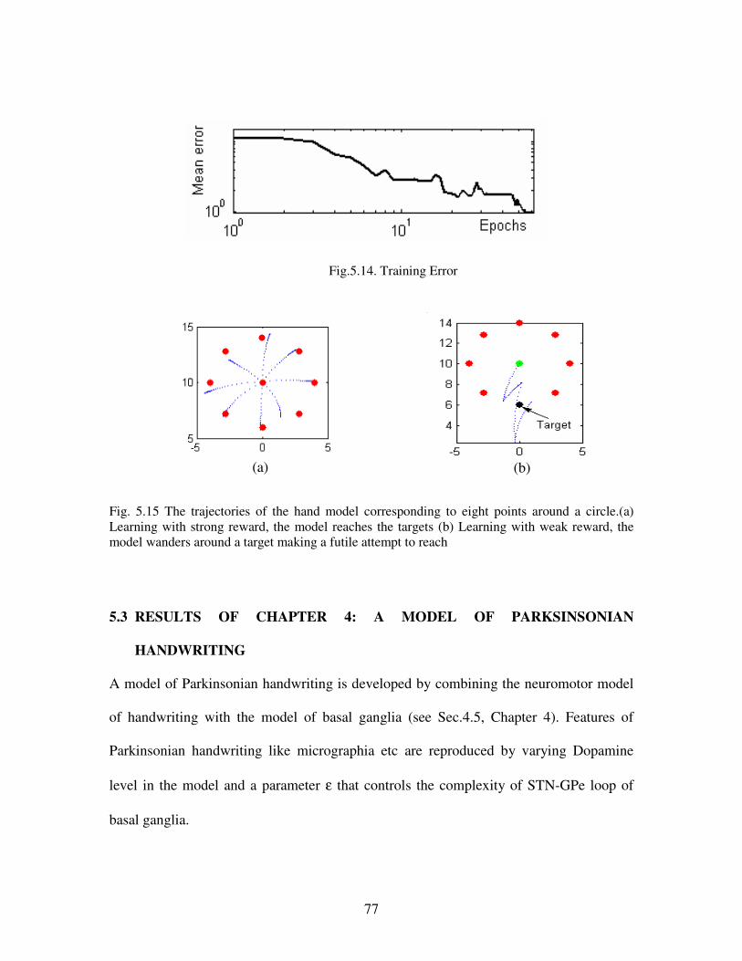
77
Fig.5.14. Training Error
Fig. 5.15 The trajectories of the hand model corresponding to eight points around a circle.(a)
Learning with strong reward, the model reaches the targets (b) Learning with weak reward, the
model wanders around a target making a futile attempt to reach
5.3 RESULTS OF CHAPTER 4: A MODEL OF PARKSINSONIAN
HANDWRITING
A model of Parkinsonian handwriting is developed by combining the neuromotor model
of handwriting with the model of basal ganglia (see Sec.4.5, Chapter 4). Features of
Parkinsonian handwriting like micrographia etc are reproduced by varying Dopamine
level in the model and a parameter ε that controls the complexity of STN-GPe loop of
basal ganglia.
(a) (b)
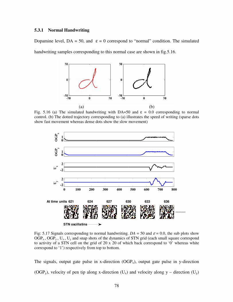
78
5.3.1 Normal Handwriting
Dopamine level, DA = 50, and ε = 0 correspond to “normal” condition. The simulated
handwriting samples corresponding to this normal case are shown in fig.5.16.
(a) (b)
Fig. 5.16 (a) The simulated handwriting with DA=50 and ε = 0.0 corresponding to normal
control. (b) The dotted trajectory corresponding to (a) illustrates the speed of writing (sparse dots
show fast movement whereas dense dots show the slow movement)
01
OG
Px
01
OG
Py
-2
2
Ux
0 100 200 300 400 500 600 700 800
-2
2
Uy
621 624 627 630 633 636At time units
STN oscillatins
Fig: 5.17 Signals corresponding to normal handwriting. DA = 50 and ε = 0.0, the sub plots show
OGPx , OGPy , Ux , Uy and snap shots of the dynamics of STN grid (each small square correspond
to activity of a STN cell on the grid of 20 x 20 of which back correspond to ‘0’ whereas white
correspond to ‘1’) respectively from top to bottom.
The signals, output gate pulse in x-direction (OGPx), output gate pulse in y-direction
(OGPy), velocity of pen tip along x-direction (Ux) and velocity along y – direction (Uy)
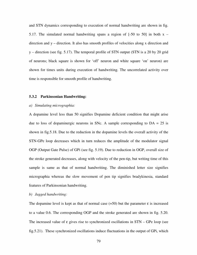
79
and STN dynamics corresponding to execution of normal handwriting are shown in fig.
5.17. The simulated normal handwriting spans a region of [-50 to 50] in both x –
direction and y – direction. It also has smooth profiles of velocities along x direction and
y – direction (see fig. 5.17). The temporal profile of STN output (STN is a 20 by 20 grid
of neurons; black square is shown for ‘off’ neuron and white square ‘on’ neuron) are
shown for times units during execution of handwriting. The uncorrelated activity over
time is responsible for smooth profile of handwriting.
5.3.2 Parkinsonian Handwriting:
a) Simulating micrographia:
A dopamine level less than 50 signifies Dopamine deficient condition that might arise
due to loss of dopaminergic neurons in SNc. A sample corresponding to DA = 25 is
shown in fig.5.18. Due to the reduction in the dopamine levels the overall activity of the
STN-GPe loop decreases which in turn reduces the amplitude of the modulator signal
OGP (Output Gate Pulse) of GPi (see fig. 5.19). Due to reduction in OGP, overall size of
the stroke generated decreases, along with velocity of the pen-tip, but writing time of this
sample is same as that of normal handwriting. The diminished letter size signifies
micrographia whereas the slow movement of pen tip signifies bradykinesia, standard
features of Parkinsonian handwriting.
b) Jagged handwriting:
The dopamine level is kept as that of normal case (=50) but the parameter ε is increased
to a value 0.6. The corresponding OGP and the stroke generated are shown in fig. 5.20.
The increased value of ε gives rise to synchronized oscillations in STN – GPe loop (see
fig.5.21). These synchronized oscillations induce fluctuations in the output of GPi, which
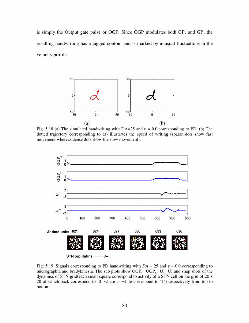
80
is simply the Output gate pulse or OGP. Since OGP modulates both GPx and GPy the
resulting handwriting has a jagged contour and is marked by unusual fluctuations in the
velocity profile.
(a) (b)
Fig. 5.18 (a) The simulated handwriting with DA=25 and ε = 0.0.corresponding to PD. (b) The
dotted trajectory corresponding to (a) illustrates the speed of writing (sparse dots show fast
movement whereas dense dots show the slow movement).
0
1
OG
Px
01
OG
Py
-2
2
Ux
0 100 200 300 400 500 600 700 800
-2
2
Uy
621 624 627 630 633 636
STN oscillatins
At time units
Fig: 5.19. Signals corresponding to PD handwriting with DA = 25 and ε = 0.0 corresponding to
micrographia and bradykinesia. The sub plots show OGPx , OGPy , Ux , Uy and snap shots of the
dynamics of STN grid(each small square correspond to activity of a STN cell on the grid of 20 x
20 of which back correspond to ‘0’ where as white correspond to ‘1’) respectively from top to
bottom.
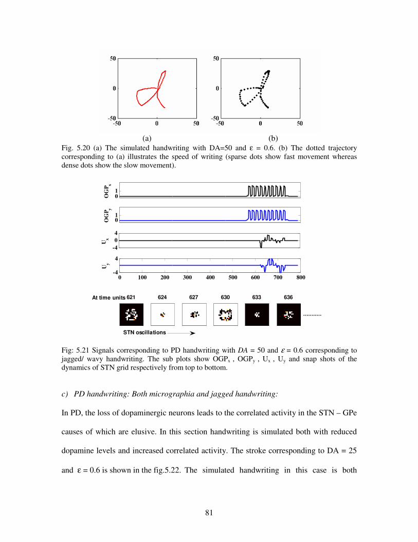
81
(a) (b)
Fig. 5.20 (a) The simulated handwriting with DA=50 and ε = 0.6. (b) The dotted trajectory
corresponding to (a) illustrates the speed of writing (sparse dots show fast movement whereas
dense dots show the slow movement).
01
OG
Px
01
OG
Py
-4
0
4
Ux
0 100 200 300 400 500 600 700 800-4
4
Uy
621 624 627 630 633 636
STN oscillations
At time units
Fig: 5.21 Signals corresponding to PD handwriting with DA = 50 and ε = 0.6 corresponding to
jagged/ wavy handwriting. The sub plots show OGPx , OGPy , Ux , Uy and snap shots of the
dynamics of STN grid respectively from top to bottom.
c) PD handwriting: Both micrographia and jagged handwriting:
In PD, the loss of dopaminergic neurons leads to the correlated activity in the STN – GPe
causes of which are elusive. In this section handwriting is simulated both with reduced
dopamine levels and increased correlated activity. The stroke corresponding to DA = 25
and ε = 0.6 is shown in the fig.5.22. The simulated handwriting in this case is both
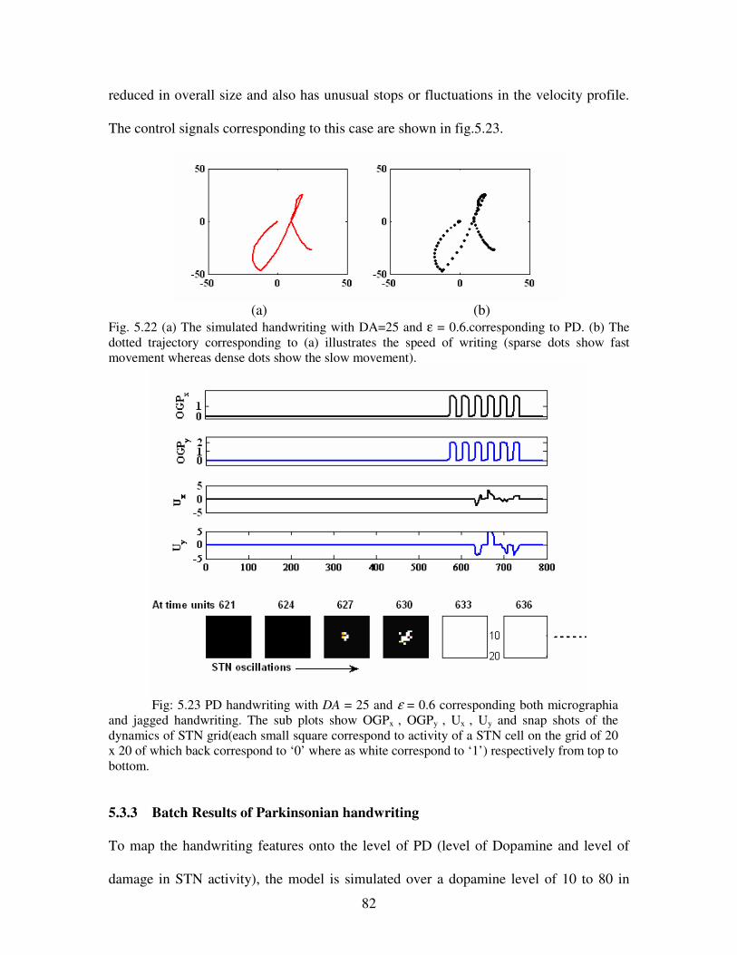
82
reduced in overall size and also has unusual stops or fluctuations in the velocity profile.
The control signals corresponding to this case are shown in fig.5.23.
(a) (b)
Fig. 5.22 (a) The simulated handwriting with DA=25 and ε = 0.6.corresponding to PD. (b) The
dotted trajectory corresponding to (a) illustrates the speed of writing (sparse dots show fast
movement whereas dense dots show the slow movement).
Fig: 5.23 PD handwriting with DA = 25 and ε = 0.6 corresponding both micrographia
and jagged handwriting. The sub plots show OGPx , OGPy , Ux , Uy and snap shots of the
dynamics of STN grid(each small square correspond to activity of a STN cell on the grid of 20
x 20 of which back correspond to ‘0’ where as white correspond to ‘1’) respectively from top to
bottom.
5.3.3 Batch Results of Parkinsonian handwriting
To map the handwriting features onto the level of PD (level of Dopamine and level of
damage in STN activity), the model is simulated over a dopamine level of 10 to 80 in
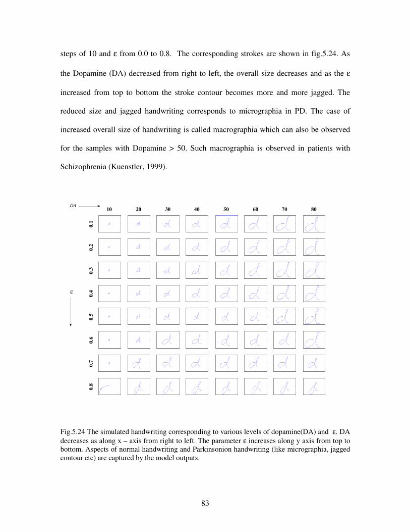
83
steps of 10 and ε from 0.0 to 0.8. The corresponding strokes are shown in fig.5.24. As
the Dopamine (DA) decreased from right to left, the overall size decreases and as the ε
increased from top to bottom the stroke contour becomes more and more jagged. The
reduced size and jagged handwriting corresponds to micrographia in PD. The case of
increased overall size of handwriting is called macrographia which can also be observed
for the samples with Dopamine > 50. Such macrographia is observed in patients with
Schizophrenia (Kuenstler, 1999).
10
0.1
20 30 40 50 60 70 80
0.2
0.3
0.4
0.5
0.6
0.7
0.8
DA
ε
Fig.5.24 The simulated handwriting corresponding to various levels of dopamine(DA) and ε. DA
decreases as along x – axis from right to left. The parameter ε increases along y axis from top to
bottom. Aspects of normal handwriting and Parkinsonion handwriting (like micrographia, jagged
contour etc) are captured by the model outputs.
84
5.4 SUMMARY
In the present chapter the results of handwriting model which aims at obtaining an
optimal way of stroke generation is presented. The issues in motor preparation and
multiple stroke generation are raised and solutions are attempted. The results of
modeling basal ganglia as a source of exploratory drive are presented. The results of the
computational model of PD handwriting, which show micrographia are discussed. The
following chapter presents the conclusions of this thesis.
.
85
CHAPTER 6
CONCLUSIONS
Chapter 2: A Neuromotor Model of Handwriting Generation
A neural network model of handwritten stroke generation in which stroke velocities are
expressed as a Fourier-style decomposition of oscillatory neural activities is presented.
Though oscillatory neural models are typically used to model generation of rhythmic
behavior like walking, swimming etc. (Marder, 1996), they proved to be useful in non-
rhythmic motor function also (Prashanth and Chakravarthy, 2003). Since Hollerbach’s
insightful observation on oscillatory elements in handwriting, neural oscillators have
figured in models of handwriting also. An oscillatory neural model of handwriting, to be
biologically viable, has to address certain fundamental issues.
The first key issue is one of preparing the initial state of the oscillatory network. This
question does not seem have received adequate attention in literature (Plamondon, 1989;
Kalveram, 1996; Shcomaker, 1991; Grossberg, 2000). Primarily the network’s internal
state must posses a stable rhythm properly registered with respect to the time of onset of
the stroke. Further there must be a mechanism to switch the network to a different, stable
rhythm to produce a different stroke. Even if the network dynamics are stable enough to
flow into a stable trajectory on random initialization, the temporal profile of the network
may not be specific enough to produce a desired behavior. There must be some level of
forgetting of initial conditions, and therefore linear oscillator models are disallowed.
Networks of nonlinear oscillators, with their proneness to chaos (Chirikov, 1979), must
be handled with extreme delicacy to produce stable, specific rhythms.
86
In the present work, we believe that a reasonable solution that addresses the above issues
is provided. The oscillatory network is initialized with small random noise, but is
immediately given a large PP to specific neurons. This pushes the evolution of all the
sublayers in a specific direction, which, after a specific delay, ∆, fall into a nearly
standard rhythm (forgetting the low-amplitude diversity in the initial conditions). A PP of
inadequate amplitude or an adequate delay (∆) after the PP will not result in the desired
output. Biological significance of this “motor delay” will be discussed later in this
chapter.
A coarse mapping of our network architecture onto neuroanatomy can be suggested. The
timing network could possibly represent either cerebellum or basal ganglia, whose role in
timing and predictive functions is well established (see fig.6.1). However, we will argue
that the actions of the timing network closely match the activities of basal ganglia. The
input layer could represent either the pre Supplementary Motor Area (preSMA) or
Premotor (PM) area where complex motor sequences are initiated. The hidden layer
could represent SMA; this region involved in preparation and initiation of movements.
The output layer may be considered as a “lumped” representation including Primary
Motor area (M1) and all the motor structures below it in motor hierarchy. The enabling
control of the timing network on the output is analogous to the “action gating” of basal
ganglia on M1 (Houk, 1995). It is well-known that striatum provides intermittent,
focused inhibition within output structures which otherwise maintain inhibitory control
over motor/cognitive systems throughout the brain (Harner, 1997).
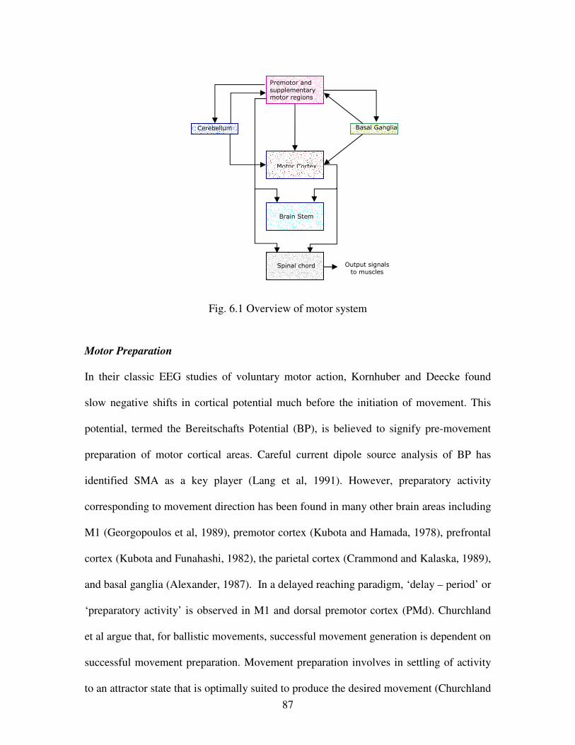
87
Fig. 6.1 Overview of motor system
Motor Preparation
In their classic EEG studies of voluntary motor action, Kornhuber and Deecke found
slow negative shifts in cortical potential much before the initiation of movement. This
potential, termed the Bereitschafts Potential (BP), is believed to signify pre-movement
preparation of motor cortical areas. Careful current dipole source analysis of BP has
identified SMA as a key player (Lang et al, 1991). However, preparatory activity
corresponding to movement direction has been found in many other brain areas including
M1 (Georgopoulos et al, 1989), premotor cortex (Kubota and Hamada, 1978), prefrontal
cortex (Kubota and Funahashi, 1982), the parietal cortex (Crammond and Kalaska, 1989),
and basal ganglia (Alexander, 1987). In a delayed reaching paradigm, ‘delay – period’ or
‘preparatory activity’ is observed in M1 and dorsal premotor cortex (PMd). Churchland
et al argue that, for ballistic movements, successful movement generation is dependent on
successful movement preparation. Movement preparation involves in settling of activity
to an attractor state that is optimally suited to produce the desired movement (Churchland
Basal Ganglia Cerebellum
Motor Cortex
Brain Stem
Output signals to muscles
Spinal chord
Premotor and
supplementary motor regions
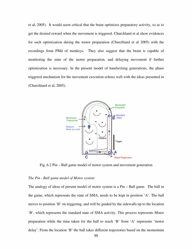
88
et al, 2005). It would seem critical that the brain optimizes preparatory activity, so as to
get the desired reward when the movement is triggered. Churchland et al show evidences
for such optimization during the motor preparation (Churchland et al 2005) with the
recordings from PMd of monkeys. They also suggest that the brain is capable of
monitoring the state of the motor preparation, and delaying movement if further
optimization is necessary. In the present model of handwriting generations, the phase
triggered mechanism for the movement execution echoes well with the ideas presented in
(Churchland et al, 2005).
Fig. 6.2 Pin – Ball game model of motor system and movement generation
The Pin - Ball game model of Motor system:
The analogy of ideas of present model of motor system is a Pin – Ball game. The ball in
the game, which represents the state of SMA, needs to be kept in position ‘A’. The ball
moves to position ‘B’ on triggering, and will be guided by the sidewalls up to the location
‘B’, which represents the standard state of SMA activity. This process represents Motor
preparation while the time taken for the ball to reach ‘B’ from ‘A’ represents ‘motor
delay’. From the location ‘B’ the ball takes different trajectories based on the momentum
Standard State
Movement Execution
Reward
Trigger
Movement Trajectories
Network State as a ball
A
Motor Preparation C
B
89
in it, representing the execution of movement (or handwritten stroke). All the trajectories
may not be rewarding which represents poor skill of execution of the movement. At the
end of the trial the ball reaches position ‘C’ which will be brought to ‘A’ for next trail. In
the dynamical systems point of view, the position ‘B’ is should be a ‘saddle node’. The
positions from ‘C’ to ‘A’ are ‘line of fixed points’ in the presence of gravity (the present
model does not incorporate these states, but motor system seems to have such states). The
trajectory corresponding to ‘C - A - B’ represents the preparatory activity. This activity
seems to be as optimal as possible for good movement generation (if this trajectory was
curved rather than being straight, the overall momentum will be less in the Pin- Ball
game). The ball at position ‘B’ represents the standard state, because of the fact that up to
this location every ball takes the same trajectory and after which it will slide into various
trajectories.
SMA and Motor Preparation
From the above account SMA seems to compete with several other motor areas as a
primary source of motor preparatory signals. Single cell recordings in primates revealed
more marked preparation-related changes in SMA neurons than in neurons of M1 (Tanji,
1994). The question can be resolved if it can be shown that preparatory activity in SMA
neurons precedes similar activity in M1. It has been shown that SMA neurons exhibiting
preparatory activity can be identified to project to M1 (Tanji et al, 1980). Contrarily, it
was also established that M1 neurons that exhibit preparatory activity receive inputs from
SMA and not from thalamus or parietal cortex (Aizawa and Tanji, 1994). Such studies
strongly implicate a role to SMA in motor preparation. However, perhaps SMA may not
be solely responsible for motor preparation. Its preparatory action might involve
90
interactions subcortical structures like basal ganglia, which are often implicated in motor
timing functions.
SMA and Basal Ganglia in Sequence Generation
Interaction between SMA and basal ganglia is believed to play a crucial role in learnt
motor sequences (Cunnington et al 1995). It has been suggested that phasic activity of
basal ganglia may act as a “reset” signal to the SMA clearing the traces after one
movement and preparing it for the consecutive movement (Georgiou et al 1993).
The above description of cortico-striatal interaction in event timing and sequence
generation is much in line with the treatment of these temporal processing mechanisms in
our model of handwriting generation. The oscillatory layer (a cortical area, most probably
SMA) is stimulated by the timing network (basal ganglia) so as to induce a stable rhythm
in the former. The timing network waits for a specific phase pattern in the oscillatory
layer and initiates stroke execution. We have seen that other ways of determining stroke
onset moment yielded suboptimal results. The two-way interaction between the timing
network and the oscillatory layer is strongly analogous to the above description of the
role of basal ganglia in timing and sequence generation.
Basal Ganglia and Motor Timing
Coordinating the relative timing of multiple streams of processing is crucial in both
motor performance and sensory perception. Temporal processing in biological systems
occurs over a range of time scales and is broadly classified into 3 categories: 1) circadian
timing, which corresponds to durations of the order of days, and handled by brain
structures like suprachiasmatic nuclei, 2) interval timing, which corresponds to durations
in the range of seconds to minutes, and coordinated primarily by corticostriatal
91
interactions, and 3) millisecond timing, which obviously corresponds to millisecond
durations, controlled by the cerebellum (Buhusi and Meck, 2005).
The role of basal ganglia in ‘interval timing’ appears to emerge from the dynamics of
thalamo-cortico-striatal loops. In a model – the Striatal Beat Frequency (SBF) model –
that highlights the timing function of basal ganglia, the cortical oscillators are assumed to
increase synchrony just before movement onset and maintain the rhythm throughout the
performance (Buhusi and Meck, 2005). The dopaminergic burst at trial onset could
trigger the synchronization of cortical oscillators according to SBF model. And the
striatal neurons are tuned to respond to specific patterns of cortical oscillations (Buhusi
and Meck, 2005).
Isochrony in Handwriting
The isochrony principle shows that duration of handwriting movement tends, within
certain limits, to be relatively independent of the length of the trajectory. The perception
of human movement is influenced by the implicit knowledge of motor rules (Viviani
1983; Thomassen and Teulings 1985). This feature is an intrinsic behavior of the current
model of handwriting generation. As the model is trained to generate all strokes in one
cycle of hidden layer oscillation, it takes almost equal time for the generation of each
stroke.
Motor variability
One of the most commonly seen features in human movement is motor variability. Motor
control researchers view it as a window into the central organization of the system that
produces voluntary movements (Latash, 2001). One of the obvious origins of motor
92
variability is motor redundancy. Variability in movement generation is a problem where
accuracy is needed and is an asset for adjusting the movement during learning. The motor
variability needs to be controlled depending on the context. For example in learning
archery one needs variability in force production and directional tuning for the release of
arrow onto the target. But after learning, for skilled archery, the learner needs to suppress
the variability.
The motor system, which is a large complex dynamical system, has all the ingredients to
generate innate variability. In the present work it is also argued that apart from the noise
in the initial conditions in the network and properties of dynamics systems, the ‘motor
preparation’ may contribute to motor variability. The preparation of the network may not
precisely land the network state exactly onto the standard state, but it confines the
network state to a narrow region around the standard state (the standard state is the state
of the network in its state space, from which the onset of a movement lead to an accurate
movement). These states in this subset act as the initial noise in the network, which may
lead to variability in the movement generation.
We are aware that our model has several simplifying assumptions. The input layer in our
model which represents inputs from source areas of handwriting information (probably
language areas in parietal cortex) and the model’s output layer which represents all motor
areas in motor hierarchy below SMA are obviously given a summary treatment. This is
because one of the key motivations of the work is to highlight the role of SMA and basal
ganglia in sequential behavior, specifically handwriting. The timing network, which
represents basal ganglia, is at the moment defined in terms of its inputs and outputs and
not defined as a neural network model. Further, the most important element of basal
93
ganglia is perhaps the dopamine signal which is thought to contain reward information.
These necessities provide direction to future extensions of the present work.
Chapter 3: The Model of Basal Ganglia
In spite of availability of extensive experimental and clinical data, the essential function
of basal ganglia (BG) continues to elude computational modelers (Harner, 197; Berns and
Sejnowsky, 1998; Houk, 1995; Montague e al 1996), as evidenced in the diversity of
existing views on the subject. Dominant thought considers BG as an Action gate that
releases and places motor resources at the disposal of commands originating from higher
motor cortical areas. BG have also been afforded roles in sequence generation and
working memory. An idea that had gained significant concurrence is that BG is involved
in motor learning by reinforcement with Dopamine as a reward signal (Montague et al,
1996; Barto, 1999). Any realization of reinforcement learning requires, in addition to a
reward signal, a noise source that can exhaustively explore the output (or action) space.
In this thesis it is proposed that the complex activity of the STN-GPe loop implements
this noise signal which accounts for the exploratory drive. It has been observed that there
is a loss of complexity (greater regularity) in the STN-GPe loop activity in dopamine
depleted conditions (Terman et al, 2002; Beyan et al, 2003; Berman et al, 1994; Nini et
al, 1995, Raz et al, 2000; Brown et al, 2001). We had suggested a possible functional
consequence of this loss of complexity and presented a view of BG as a source of
exploratory drive for reinforcement based motor learning with an enhanced model of BG
involved in reaching. When there is a reliable dopamine-based reward signal the model
successfully learns to reach, and when the signal is absent the arm wanders around the
target failing to reach.
94
Basal Ganglia as a Source of Exploratory Drive: Consolidation Exploration
The proposed model is a neural network architecture consisting of two parallel pathways.
We rename these pathways, traditionally called “direct” and “indirect” pathways, as
“consolidation” and “exploration” pathways. The consolidation pathway from striatum to
GPi consists of learnable connections that represent the sensory-motor map involved in
reaching task. The exploratory pathway consisting of the STN-GPe loop is a network of
oscillatory neurons; internal connections among the oscillators are designed such that the
STN-GPe loop produces chaotic activity (similar to the model of STN-GPe in Terman et
al 2002). Output of the loop to GPi provides the “noisy” or exploratory signal necessary
for reward-based learning. Reward signal, representing dopamine, from Substantia Nigra
compacta (SNc) is projected onto striatum which selects between the consolidation
pathway and the exploratory pathway depending on the reward level. When the reward is
low, the exploratory pathway is selected. Complex activity of STN-GPe loop, then,
explores the output space, resulting in exploratory movement of the arm. When the
exploring arm chances upon the target, the system receives a strong reward signal, the
consolidation pathway is selected (the exploratory drive is suppressed) and the
connections between striatum and GPi are reinforced in a Hebb-like fashion.
Chaotic Oscillations in STN – GPe Activity and Reinforcement Learning:
The presence of chaotic (uncorrelated activity) in BG in normal rats and correlated
activity in Rat models of PD are reported by Terman et al (2002). What is the functional
significance of chaos in basal ganglia? How chaos helps in healthy controls in daily
living? What is the role of chaos in BG in learning? What function could natural,
ubiquitous chaos serve?
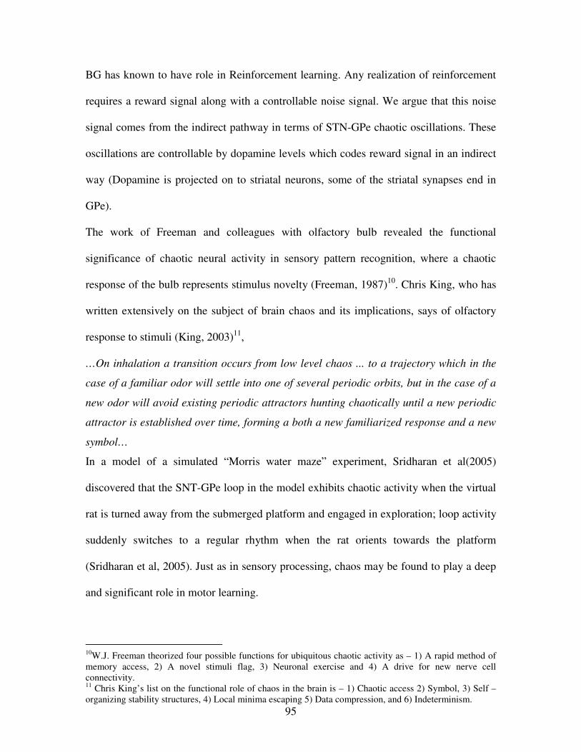
95
BG has known to have role in Reinforcement learning. Any realization of reinforcement
requires a reward signal along with a controllable noise signal. We argue that this noise
signal comes from the indirect pathway in terms of STN-GPe chaotic oscillations. These
oscillations are controllable by dopamine levels which codes reward signal in an indirect
way (Dopamine is projected on to striatal neurons, some of the striatal synapses end in
GPe).
The work of Freeman and colleagues with olfactory bulb revealed the functional
significance of chaotic neural activity in sensory pattern recognition, where a chaotic
response of the bulb represents stimulus novelty (Freeman, 1987)10
. Chris King, who has
written extensively on the subject of brain chaos and its implications, says of olfactory
response to stimuli (King, 2003)11
,
…On inhalation a transition occurs from low level chaos ... to a trajectory which in the
case of a familiar odor will settle into one of several periodic orbits, but in the case of a
new odor will avoid existing periodic attractors hunting chaotically until a new periodic
attractor is established over time, forming a both a new familiarized response and a new
symbol…
In a model of a simulated “Morris water maze” experiment, Sridharan et al(2005)
discovered that the SNT-GPe loop in the model exhibits chaotic activity when the virtual
rat is turned away from the submerged platform and engaged in exploration; loop activity
suddenly switches to a regular rhythm when the rat orients towards the platform
(Sridharan et al, 2005). Just as in sensory processing, chaos may be found to play a deep
and significant role in motor learning.
10
W.J. Freeman theorized four possible functions for ubiquitous chaotic activity as – 1) A rapid method of
memory access, 2) A novel stimuli flag, 3) Neuronal exercise and 4) A drive for new nerve cell
connectivity. 11
Chris King’s list on the functional role of chaos in the brain is – 1) Chaotic access 2) Symbol, 3) Self –
organizing stability structures, 4) Local minima escaping 5) Data compression, and 6) Indeterminism.
96
Chapter 4: A Model of Pd Handwriting
Recognition of rich diagnostic value of handwriting had prompted a systematic study of
handwriting and the extensive neuromotor organization that generates it. Handwriting can
be used a source of diagnostic information in neurological disorders like in Obsessive
Compulsive disorder (Marvogiorgou et al, 2001), Schizophrenia (Gallucci et al, 1997),
cortical dysfunction in old age (Erricson et al, 1991), Dysgraphia and Dyslexia
(Rosenblum, 2003) and Parkinson’s disease (Teulings et al, 1991and Philip et al, 1991) .
Handwriting in Parkinson’s disease
Parkinsonian handwriting is typically characterized by micrographia, jagged line contour,
and unusual fluctuations in the velocity of pen tip. Attempts have been made to use
quantitative parameters of Parkinsonian handwriting to determine appropriate drug
dosage. However most such attempts treat the motor system as a “black box” and are
based on an empirical relationship between the handwriting parameters and the stage of
maturity of the disease. However, since impairment of basal ganglia function underlies
Parkinson’s disease, an insight into the understanding of basal ganglia function and the
precise role of these nuclei in handwriting generation is indispensable to produce an
accurate computational model.
The current model of Parkinsonian handwriting generation maps the handwriting features
like stroke size onto the dopamine levels empirically. Jagged line contour in handwriting
are claimed to be due to the synchronized oscillations of STN – GPe dynamics. Apart
from the above features, the model captures few other PD symptoms like,
97
1) Micrographia: The depletion of dopamine in the model shows handwriting with
micrographia features. The overall size of the stroke becomes smaller as one
decreases the dopamine. Van Gemmert et al with experimental studies on PD patients
show evidence for the significantly smaller strokes than normal controls (Van
Gemmert et al, 2005). They also report that the decreased mean acceleration and
diminished peak velocity in PD patients.
2) Bradykinesia: As isochrony is the model’s intrinsic property, the model generates all
the strokes in more or less same time. In dopamine depletion conditions the model
takes same time as that of normal time. So the overall movement is slower. Van
Gemmert et al with experiment studies found that the average stroke duration of the
patients with PD was no longer than the average stroke duration of normal
controls(Van Gemmert et al, 2005)
3) Tremor in handwriting (Waverly handwriting): Tremor in handwriting can be
observed by decrease of complex activity of the STN-GPe loop. Low frequency
synchronous burst activity in STN – GPe loop may be propagated down the motor
system which contributes to jagged handwriting.
The conclusions from the above model shows some applications could to be useful in
assisting Clinicians and surgeons and computational modelers by answering the
following questions,
1) Is it possible to map the handwriting features onto the severity of PD and the nuclei
that is dysfunctioning? Solutions to this question might be useful in finding target
nuclei for Deep Brain Stimulation (DBS) for Parkinson’s disease.
98
2) Can we use the handwriting for monitoring the effect of drugs on PD patient? Stein
suggests that changes in handwriting can be used to help monitor drug dose in various
disorders (Stein, 2001). Computer analysis of handwriting dynamics during
Dopamimetic tests in Parkinson’s disease by Cobbah and Faihrust (2000) shows that
there are positive responses to drugs. Studies of dynamic descript-characteristics of
PD handwriting have clearly shown potential in identifying various stages of PD
(Cubbah and Fairhrust, 2000).
3) How does motor system use extensive noise in the indirect pathway of BG for leaning
handwriting? Will this noise helps in learning proper movement synergies for
handwriting sequence execution?
Handwriting as a Source of Diagnostic Information
The developments in data collection technology now permit the examination of set of
handwriting outcome measures. With the aid of a digitizing tablet and instrumented pen a
subject’s handwriting can be monitored in real time with kinetic and kinematic analysis
(Rosenblum, 2001and Rosenblum, 2003). Subtle changes in person’s handwriting might
reveal neurological and psychiatric conditions years before other symptoms (of a
neurological or psychiatric disease) become obvious (Persuad, 2002). Multiple sclerosis,
dementia, Parkinson’s disease, Huntington’s chorea, Schizophrenia and obsessive
compulsive disorder are just some of the conditions that affect handwriting in specific
ways12
(Persuad, 2002). Rosenblum et al proposed the temporal measures of poor and
12
A written diagnosis (Persuad, 2002): PARKINSON’S DISEASE: patients write smaller and more slowly than healthy controls. Acceleration phases are
significantly lower.
HUNTINGTON’S CHOREA: lower and less consistent writing speed and a tendency for less consistent strokes length.
SCHIZOPHRENIA: in consistent repetitive hand movements. Mean stroke duration and time spent in acceleration and
are significantly longer.
99
proficient handwrites (children) as: i) total time to complete each task, ii) ‘in air’ time,
and iii) mean writing speed. These measures found useful for dyslexic and Dysgraphic
and ADHD (Attention Deficit Hyperactive Disorders). The temporal features of
handwriting observed in OCD are i) lower peak velocity (Bradykinesia), ii)
Micrographia, iii) shortened acceleration phase per stroke, and iv) repetition of strokes
(Marvogiorgou et al, 2001). Similarly patients with cerebellar damage show typical
features of Dysgraphia, manifested as omission and repetition of stroke and letters.
Simple geometric shape drawing tasks are commonly used to diagnose and monitor
patient performance for a range of clinical and neuropsychological conditions (Guest et
al, 2000). Erricson et al (1991) uses graphic skills as an instrument for detecting higher
cortical dysfunctions in old age. The skills suggested are like, (i) copying tasks (3D cube,
a circle, two rectangles, a rhombus and two pentagons), (ii) handwriting ability (writing a
spontaneous sentence and writing from dictation), and (iii) free-hand figurative drawing
(a dressed man or woman from the front). Gallucci et al (1997) suggest stroke
characteristics (duration and length), stroke consistency (duration and length), stroke
trajectory (efficiency and skew) and preservation for diseases related BG dysfunction like
Parkinson’s disease, Huntington’s disease also for Schizophrenia (Galucci, 1997). Philips
et al suggested stroke length, duration, peak velocity and a skew ness coefficient (a value
of 0.5 indicates equal periods of time spent in accelerative and decelerative phase of
movement) for Huntington’s disease (Philips et al, 1995).
DEMENTIA OF ALZEHEMERLS TYPE: patients write less efficiently, with more cycles of acceleration and
deceleration per writing stroke.
MULTIPLE SCELEROSIS: writing speed is reduced and stroke duration is increased. The profile of pen speeds
associated with a single stroke is irregular and multi peaked, but stroke size is in normal range.
100
Handwriting features like, stroke size, peak acceleration, and stroke duration can be used
for diagnosis of Parkinson’s disease (Teulings et al 1991, van Gemmert et al, 2003).
Philip et al suggested measures of the quality of handwriting for the analysis of PD: (i)
The ratio between mean and standard deviation of stroke length or duration; (ii) The
average number of zero crossings in acceleration relative to velocity functions; (iii) The
average number of zero crossings in jerk relative to velocity functions; and (iv) The
velocity frequency spectra.
There is no standardized measure or test battery for Parkinson’s disease. The test battery
for neurological disorders based on handwriting needs to be unified with the extensive
understanding of spatial and temporal features of handwriting and the visuo-motor
systems which generates and modulates it.
101
REFERENCES
1. Aizawa, H. and J. Tanji (1994) Cortico-cortical and thalamo-cortical responses of
neurons in the monkey primary motor cortex and their relation to a trained motor task, J
Neurophysiol, 71, 550–560.
2. Alexander, G. E. (1987) Selective neuronal discharge in monkey putamen reflects
intended direction of planned limb movements. Exp. Brain Res., 67, 623-634, 1987.
3. Alexander, G. E. Basal ganglia pp. 139-144. In The Handbook of Brain Theory and
Neural Networks, Arbib., M.A.(ed.) MIT Press, Cambridge,1995.
4. Barto, A.G. and P. Anandan (1985) Pattern recognizing stochastic learning automata.
IEEE Transactions on Systems, Man and Cybernetics, 15, 360-374.
5. Barto, AG. (1999) Reinforcement Learning. In The Handbook of Brain Theory and
Neural Networks Arbib, M.A. (ed.) Cambridge, MA: MIT Press.
6. Bergman, H., A. Feingold, A. Nini, A. Raz, H. Slovin, M. Abeles and E. Vaadia (1998) Physiological aspects of information processing in the basal ganglia of normal and
parkinsonian primates. Trends in Neuroscience, 21, 32-38, 1998.
7. Bergman, H., T. Whichman, B. Karmon, M.R. DeLaong (1994) The primate
subthalamic nucleus. II. Neural activity in MPTP model of Parkinsonism. J
Neurophysiol, 72, 507-520.
8. Berns, G.S., T.J. Sejnowski (1998) A computational model of how the Basal Ganglia
produce sequences. Journal of Cognitive Neuroscience, 10(1), 108-121.
9. Bevan, M.D., P.J. Magill, D. Terman, J.P. Bolam and C.J. Wilson (2003) Move To
The Rhythm: Oscillations In The Subthalamic Nucleus-External Globus Pallidus
Network. Trends in Neuroscience (in press)
10. Bhuhusi, C.V. and W.H. Meck (2005) What makes us tick? Functional and neural
mechanisms of interval timing Nature reviews neuroscience, 6, 755.
11. Bilney, B., M.E. Morris and D. Sonia (2003) Physiotherapy for people with movement
disorders arising from basal ganglia dysfunction. NZ journal of Physiotherapy, 31, 2.
12. Bjorne, P. and C. Balkenius (2005) A model of attentional impairments in autism: First
steps toward a computational theory. Cognitive Systems Research, 6(3), 193-204.
13. Borrett, D.S., T.H. Yeap and H.C. Kwan (1993) Candian Journal of Neurological
Sciences 20,107.
14. Bressloff, P.C., S. Coombes, and B. Souza (2002) Dynamics of a Ring of Pulse-
Coupled Oscillators: Group Theoretic Approach. Phys Rev E Stat Nonlin. Soft. Matter.
Phys. 66.
15. Brown, P., A. Olivero, P. Mazzone, A. Insola, P. Tonali, V.D. Lazzaro (2001)
Dopamine dependency of oscillations in between subthalamic neucleus and pallidum in
Parkinson’s disease. J Neurosci, 21, 1033-1038.
16. Buhusi, C.V., W.H. Meck (2005) What makes us tick? Functional and neural
mechanisms of interval timing. Nat. Rev. Neurosci. 6 (10):755-6
17. Bullock, D. and S. Grossberg (1988) The VITE: a neural command circuit for
generating arm and articulator trajectories. In dynamic patterns in complex systems,
Kelso, A. and Shlesinger, M.M. (eds), Singapore: world Scientific. (1988).
18. Bullock, D., R.M. Bongers, M. Lankhorst P.J. Beek (1999) A vector-integration-to-
endpoint model for performance of viapoint movements. Neural Netw.12 (1), 1-29.
19. Chirikov, B. (1979) A universal instability of many – dimensional oscillator systems,
Phy.Rev., 52, 263-379.
102
20. Churchland, M.M., M.Y. Byron and I.R. Stephen, G. Santhanam, A. Afshar, V.S. Krishna (2005) Neural variability in premotor cortex provides a signature of motor
preparation. In the proceedings of COSYNE , March.
21. Churchland, P. and T.J. Sejnowski The Computational Brain MIT Press, Cambridge,
Massachusetts, 1992
22. Cobbah, W.G.K. and M.C. Fairhurst (2000) Computer analysis of handwriting
dynamics during dopamimetic tests in Parkinson's disease. EUROMICRO. 2414-2418.
23. Crammond, D. J., and J. F. Kalaska (1989) Neuronal activity in primate parietal cortex
area 5varies with intended movement direction during an instructed – delay period. Exp.
Brain Res. 76, 458- 462.
24. Crystal, H., L.H. Finkel Computational approaches to neurological disease. In Reggia,
J.A., E. Ruppin, R.S. and Berndt (eds.) Neural Modeling of Brain and Cognitive
Disorders. Singapore: World Scientific, 1996.
25. Cunnington, R., R. Iansek, J. A. Bradshaw and J.G. Phillips (1995) Movement-
related potentials in Parkinson’s disease: Presence and predictability of temporal and
spatial cues, Brain, 118, 935-950.
26. Dayan, P and L.F. Abbot Theoretical Neuroscience: Computational and Mathematical
modeling of neural systems, MIT press , Cambridge, Massachusetts, 2001.
27. Dominey, P., M. Arbib, and J.P. Joseph (1995)A model of cortico striatal Plasticity for
learning oculomotor associations and sequences. Journal of Cognitive Neuroscience, 7 (3), 311-336.
28. Ellis, A.W. Modeling the writing process. In Perspectives in cognitive neuropsychology,
Denes, G, C. Semenza, P. Bisiacchi and E. Andreewsky(eds.) London: Erlbaum, 1986.
29. Ericsson, K., L. Forssell, K. Amberla, K. Holmén, M. Viitanen and B. Winblad (1991) Graphic skills used as an instrument for detecting higher cortical dysfunctions in
old age, Human Movement Science , 10( 2-3), 335-349.
30. Fiala, J., S. Grossberg, D. Bullock (1996) Metabotropic glutamate receptor activation
in cerebellar Purkinje cells as substrate for adaptive timing of the classically conditioned
eye-blink response. The Journal of Neuroscience, 16, 3760-3774.
31. Gallucci, R.M., J.G. Phillips, J.L. Bradshaw, K.S. Vaddadi and C. Pantelis (1997)
Kinematic analysis of handwriting movements in schizophrenic patients. Biol.
Psychiatry. 41 (7), 830-833.
32. Georgiou, N., R. Iansek , J.L. Bradshaw, J.G. Phillips, J.B. Mattingley and J. A. Bradshaw (1993) An evaluation of the role of internal cues in the pathogenesis of
parkinsonian hypokinesia. Brain, 116, 1575-1587.
33. Georgopoulos, A.P., J.T. Lurito, M. Petrides, A.B. Schwartz, and J.T. Massey (1989)
Mental rotation of the neuronal population vector. Science, 243, 234-236.
34. Grossberg, S. and R.W. Paine (2000) A neural model of corticocerebellar interactions
during attentive imitation and predictive learning of sequential handwriting movements,
Neural Networks, 13, 999-1046.
35. Grossberg, S. and D. Seidman (2006) Neural dynamics of autistic behaviors: Cognitive,
emotional, and timing substrates. Psychological Review, in press.
36. Grossberg, S. Neural models of normal and abnormal behavior: what do schizophrenia,
parkinsonism, attention deficit disorder, and depression have in common? pp. 375-406.
In Reggia, J.A., E. Ruppin, D.L. Glanzman (eds.) Disorders of Brain, Behavior, and
Cognition: The Neurocomputational Perspective New York: Elsevier, 1999.
37. Guest, R.M., M.C. Fairhurst and J.M. Potter (2000) Automated Extraction of Image
Segments from Clinically Diagnostic Hand-Drawn Geometric Shapes, euromicro,
Proceedings of The 26th EUROMICRO Conference 2, 2440,
103
38. Gurney, K., T. J. Prescott and P. Redgrave (2001) A computational model of action
selection in the basal ganglia I. A new functional anatomy. Biological Cybernetics, 84,
401-410.
39. Guttman, M., J.K. Stephen and Y. Furukawa (2003) Current concepts in the
diagnosis and management of Parkinson's disease CMAJ, 168 (3).
40. Harm, M.W. and M.S. Seidenberg (1999) Phonology, Reading Acquisition, and
Dyslexia: Insights from Connectionist Models. Psychological Review, 106 (3), 491-528.
41. Harner, A.M. (1997) An Introduction to Basal Ganglia Function. Boston University,
Boston, Massachusetts
42. Haykin. S. Neural Networks: A Comprehensive Foundation, Prentice Hall PTR, July
1998,
43. Hertz, J., A. Krogh, and R.G. Palmer Introduction to the Theory of Neurocomputing,
Addison-Wesley, Reading, MA, 1991.
44. Hollerbach, J.M. (1981) An oscillation theory of handwriting. Biological Cybernetics,
(156)39, 139.
45. Horn, D. and E. Ruppin (1995). Compensatory mechanisms in an attractor neural
network model of schizophrenia. Neural Computation, 7, 182-205.
46. Houk, J. C., J. L. Davis, and D. G. Beiser (1995). Models of Information Processing in
the Basal Ganglia. Cambridge, MA, MIT Press
47. Jennings, C and S. Aamodt (2000) Computational approaches to brain function. Nature
Neuroscience, 3, 1160.
48. Kalveram, K. Th. (1996) A neural oscillator model learning given trajectories, or how
an allo-imitation algorithm can be implemented into a motor controller. In Motor control
and human skill: A multi-disciplinary perspective, J. Piek (Hrsg.) eds. Champaign:
Human Kinetics. 1996
49. Klopf, A.H., The Hedonistic Neuron: A Theory of Memory, Learning, and Intelligence.
Hemisphere, Washington, D.C., 1982.
50. Kornhuber, H.H. and L. Deecke (1990) Readiness for movement – The Bereitschafts
potential-Story Current Contents Life Sciences, 33, 22.
51. Kubota, K. and I. Hamada (1978) Visual tracking and neuron activity in the post –
arcurate area in monkeys. J. Phyiol. Paris. 74, 297-312.
52. Kubota, K. and S. Funahashi (1982) Neuron activities of monkey prefrontal cortex
during the learning of visual discriminations tasks with Go/No-Go performances.
Neurosci. Res., 3,106-129.
53. Kuenstler, U., U. Juhnhold, W. H. Knapp, and H.J. Gertz (1999) Positive correlation
between reduction of handwriting area and D2 dopamine receptor occupancy during
treatment with neuroleptic drugs. Psychiatry Research: Neuroimaging, 90 (1), 31-39.
54. Lang, W., R. Cheyne, R. Kristeva, R. Beistener, G. Lindinger and L. Deeke (1991)
Three dimensional localization of SMA activity preceding voluntary movement: a study
of electric and magnetic fields in a patient with inflation of the right supplementary motor
area. Exp. Brain Res., 87,688-695.
55. Latash, M.L., J.F. Scholz, F. Danion, and G. Schöner (2001) Structure of motor
variability in marginally redundant multi-finger force production tasks. Exp. Brain
Res.141, 53–165.
56. Marder, E., and R. L. Calabrese (1996) Principles of rhythmic motor pattern
production Physiological Reviews, 76,687–717.
57. Martin, K.E., J.G. Phillips, R. Iansek, J.L. Bradshaw(1994) Inaccuracy and
instability of sequential movements in Parkinson’s disease. Exp. Brain. Res. 102, 131–40.
58. Mavrogiorgou, P., R. Mergl, P. Tigges, J.E. Husseini, A. Schröter, G. Juckel, M. Zaudig, U. Hegerl (2001) Kinematic analysis of handwriting movements in patients with
obsessive-compulsive disorder. J Neurol Neurosurg Psychiatry70, 605-612.
104
59. Mink, J.W. (1996) The basal ganglia: Focused selection and inhibition of competing
motor programs. Progress in Neurobiology, 50 (4), 1009-1023.
60. Montague, P.R., P. Dayan and T.K. Sejnowski, (1996) A framework for
mesencephalic dopamine systems based on predictive Hebbian learning. Journal of
Neuroscience, 16, 1936-1947.
61. Montague, R., P. Dayan, and T.J. Sejnowski (1996). A Framework for
Mesencephalic Dopamine Systems Based on Predictive Hebbian Learning, The Journal
of Neuroscience, 16 (5):1936-1947.
62. Nini. A., A. Feingold, H. Slovin and H. Bergman (1995) Neurons in the Globus
pallidus do not show correlated activity in the normal monkey, but phase locked
oscillations appear in the MPTP model of parkinsonism. J. Neurophysiol, 74, 1800-1905.
63. Persuad, R. (2002) New Scientist.9, 40-42.
64. Phillips, J. G., G. E. Stelmach and N. Teasdale (1991) What can indices of handwriting
quality tell us about Parkinsonian handwriting? Human Movement Science, 10 (2-3), 301-
314.
65. Plamondon, R. (1989) An evaluation of motor models of handwriting. IEEE
Transactions on Systems, Man and Cybernetics.9 (5), 1060-1072.
66. Plamondon, R. and W. Guefali (1998) The generation of handwriting with delta
lognormal synergies, Biological Cybernetics, 78, 119-132.
67. Prashanth, P.S., and V.S. Chakravarthy (2006) An oscillator theory of motor unit
recruitment in skeletal muscle. To appear in Biological Cybernetics.
68. Prescott, T. J., K. Gurney, and Redgrave, P. (2002). Basal ganglia. In M. A. Arbib
(ed.) The Handbook of Brain Theory and Neural Networks (2nd Edition). Cambridge,
MA: MIT Press.
69. Prunier, C., E. Bezard, J. Montharu, M. Mantzarides, J.C. Besnard, J.L. Baulieu, C. Gross, D. Guilloteau and S. Chalon (2003) Presymptomatic diagnosis of experimental
Parkinsonism with I-PE2I SPECT. NeuroImage, 19, 810–816.
70. Raz, A., Vaadia, E. and H. Bergman (2000) Firing patterns of spontaneous discharge of
pallidal neurons in the model of Parkinsonism. J Neurosci, 20, 8559-8571.
71. Redgrave, P., T.J. Prescott and K. Gurney (1999) The basal ganglia: a vertebrate
solution to the selection problem? Neuroscience, 89, 1009-1023.
72. Reggia, J, E., Ruppin and R. Berndt Neural Modeling of Brain and Cognitive
Disorders. World Scientific. 1996.
73. Rescorla, R. A., and A.R. Wagner (1972) A theory of Pavlovian conditioning:
Variations in the effectiveness of reinforcement and nonreinforcement. pp. 64-99. In
Classical conditioning II: Current research and theory Black, A. H., and W. F. Prokasy (eds), New York: Appleton-Century-Crofts.
74. Reynolds, J. N., B.I. Hyland, and Wickens, J. R. (2001) A cellular mechanism of
reward-related learning. Nature 413, 67-70.
75. Riederer, P., Wuketich, S. (1976) Time course of nigrostriatal degeneration in
Parkinson’s disease. J. Neural Transm. 38, 277–301.
76. Rosenblum, S., S. Parush and P.L. Weiss (2001) Temporal measures of poor and
proficient handwriters, In Meulenbroek., R.G.J. and B. Steenbergen (eds), Proceedings
of Tenth biennial conference of the IGS, University of Nijmegen The Nether Lands, 119-
125.
77. Rosenblum, S., S. Parush, L. Epsztein, and P.L Weiss (2003) Process Versus Product
Evaluation of Poor Handwriting among Children with Developmental Dysgraphia and
ADHD, In Teulings, H.L., and A.W.H Van Gemmert, Proceedings of 11th conference
of the IGS, USA; Scottsdate Arizona. 169-173.
105
78. Ruppin, E., D. Horn, N. Levy, and J. Reggia Computational Studies of Synaptic
Alterations in Alzheimer's Disease. In Reggia, J., E. Ruppin, & R. Berndt (eds.),
Neural Modeling of Brain and Cognitive Disorders, World Scientific. (1996)
79. Ruppin. E., J.A. Reggia and D. Glanzmann (1999) Understanding brain and cognitive
disorders: the computational perspective, Prog. Brain. Res., 121, ix-xv.
80. Schomaker, L.R.B. (1991) Simulation and recognition of handwriting movements: a
vertical approach to modeling human motor behavior, PhD thesis, Nijmegen University,
Netherlands,
81. Silva, L. F. H. and J.P. Pijn Epilepsy: Network models of generation pp. 367-369. In
Arbib.. M. (ed.) The handbook of brain theory and neural networks. Cambridge, MA:
MIT Press. 1995.
82. Silveri, M.C., S. Misciagna, M.G. Leggio and M. Molinari (1999) Cerebellar spatial
dysgraphia: further evidence. J Neurol. 246 (4), 312-3.
83. Singhala, B., J. Lalkakaa and C. Sankhlab (2003) Epidemiology and treatment of
Parkinson’s disease in India, Parkinsonism and Related Disorders 9, 105–109.
84. Skarda, C. A., and W. J. Freeman (1987). How brain makes chaos in order to make
sense of the world. Behavioral and Brain Sciences, 10,161-195.
85. Sridharan, D., P.S. Prashanth and V.S. Chakravarthy (2005) On the Exploratory
Role of complex oscillations in a model of Basal Ganglia based on Reinforcement
Learning. To appear in Journal of Neural Engineering.
86. Stein, D.J. (2001) Handwriting and obsessive-compulsive disorder. Lancet. 18,
358(9281):524-5.
87. Sutton. R.S. and A.G. Barto Reinforcement Learning: An Introduction. MIT Press,
1999.
88. Tanji, J. (1994) The supplementary motor area in the cerebral cortex. Neurosci Res.19
(3), 251–268.
89. Tanji, J., K. Taniguchi, and T. Saga (1980) Supplementary motor area: neuronal
response to motor instructions. J. Neurophysio., 43, 60–68.
90. Terman, D., J.E. Rubin, A.C. Yew and C.J. Wilson (2002) Activity Patterns in a
Model for the Subthalamopallidal Network of the Basal Ganglia. J Neurosci, 22 (7),
2963-2976.
91. Tesauro, G. (1992) Practical issues in temporal difference learning. Machine Learning, 8,
257--277.
92. Teulings HL, C.J.L. Vidal, G.E. Stelmach and C.H. Adler (2002) Handwriting size
adaptation under distorted visual feedback in Parkinson’s disease patients, elderly
controls and young controls, Journal of Neurology, Neurosurgery, and Psychiatry,
72(3):315-324.
93. Teulings, H.L. and G.E. Stelmach (1991) Control of stroke size, peak acceleration, and
stroke duration in Parkinsonian handwriting. Human Movement Science 10, (2-3), 315-
334.
94. Teulings, H.L., A.J.W.M. Thomassen, L.R.B. Schomaker, and P. Morasso (1986)
Experimental protocol for cursive script acquisition: The use of motor information for the
automatic recognition of cursive script. In Report 3.1.2., ESPRIT project, 419.
95. Thomassen, A., H. Teulings Time, size, and shape in handwriting: exploring spatio-
temporal relationships at different levels In: Michon, J., and Jackson, J. (eds.), Time,
Mind, and Behavior, Springer-Verlag, 1985.
96. Thorndike, E.L (1911), Animal Intelligence, Macmillan press.
97. van Galen, G. and J. Weber (1998) On-line size control in handwriting demonstrates
the continuous nature of motor programs, Acta Psychologica, 100,195-216.
106
98. Van Gemmert, A. W. A., C.H. Adler, and G.E. Stelmach (2003) Parkinson's disease
patients undershoot target size in handwriting and similar tasks. Journal of Neurology,
Neurosurgery, and Psychiatry, 74, 1502-1508.
99. Van Gemmert, A.W.A., H.L., Teulings, J.L Contreras –Vidal and G.E. Stelmach (1999) Parkinson’s disease and the control of size and speed in handwriting’,
Neuropsychologica 37, 685-694.
100. Vidal, C.J., H. Teulings and G. Stelmach a Neural Network Model of Movement
Production in Parkinson's disease and Huntington's disease. In Reggia, J.A, E. Ruppin,
and R. Berndt (eds.), Neural Modeling of Brain and Cognitive Disorders, World
Scientific, 1996.
101. Vidal, J.L and G.E. Stelmach (1995) A neural model of basal ganglia-thalamocortical
relations in normal and Parkinsonian movement. Biological Cybernetics, 73, 467-476.
102. Vidal, J.L. and G.E. Stelmach (1996) Effects of Parkinsonism on motor control. Life
Sciences, 58, 165-176.
103. Viviani, P. and G. McCollum (1983) The relation between linear extent and velocity in
drawing movements. Neuroscience. 10 (1), 211-8.
104. Watkins, C. J. C. H. Learning with Delayed Rewards, Ph.D. thesis, Cambridge
University, Psychology Department, 1989.
105. Widrow, B., N. K. Gupta, and S. Maitra (1973) Punish /reward: Learning with a critic
in adaptive threshold systems. IEEE Transactions on Systems, Man, and Cybernetics 5,
455-465.
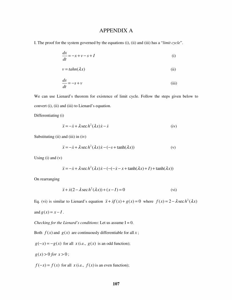
107
APPENDIX A
I. The proof for the system governed by the equations (i), (ii) and (iii) has a “limit cycle”.
dx
x v s Idt
= − + − + (i)
( )v tahn xλ= (ii)
ds
s vdt
= − + (iii)
We can use Lienard’s theorem for existence of limit cycle. Follow the steps given below to
convert (i), (ii) and (iii) to Lienard’s equation.
Differentiating (i)
2sec ( )x x h x x sλ λ= − + −�� � � � (iv)
Substituting (ii) and (iii) in (iv)
2sec ( ) ( tanh( ))x x h x x s xλ λ λ= − + − − +�� � � (v)
Using (i) and (v)
2sec ( ) ( ( tanh( ) ) tanh( ))x x h x x x x x I xλ λ λ λ= − + − − − − + + +�� � � �
On rearranging
2(2 sec ( )) ( ) 0x x h x x Iλ λ+ − + − =�� � (vi)
Eq. (vi) is similar to Lienard’s equation ( ) ( ) 0x xf x g x+ + =�� � where 2( ) 2 sec ( )f x h xλ λ= −
and ( )g x x I= − .
Checking for the Lienard’s conditions: Let us assume I = 0.
Both ( )f x and ( )g x are continuously differentiable for all x ;
( ) ( )g x g x− = − for all x (i.e., ( )g x is an odd function);
( ) 0 0g x for x> > ;
( ) ( )f x f x− = for all x (i.e., ( )f x is an even function);
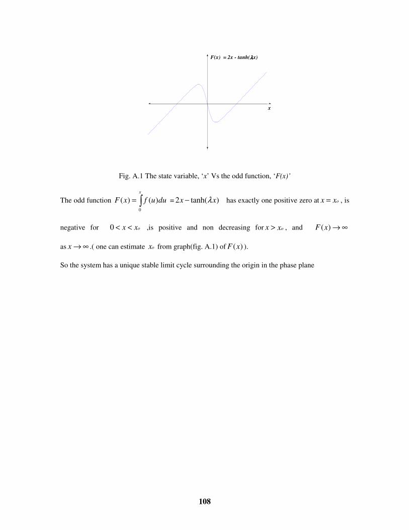
108
x
F(x) = 2x - tanh(λλλλx)
Fig. A.1 The state variable, ‘x’ Vs the odd function, ‘F(x)’
The odd function
0
( ) ( )
x
F x f u du= ∫ = 2 tanh( )x xλ− has exactly one positive zero at ox x= , is
negative for 0 ox x< < ,is positive and non decreasing for ox x> , and ( )F x → ∞
as x → ∞ .( one can estimate ox from graph(fig. A.1) of ( )F x ).
So the system has a unique stable limit cycle surrounding the origin in the phase plane
CURRICILUM VITAE
1. NAME : Garipelli Gangadhar email: [email protected]
2. DATE OF BIRTH : 04 January 1980
3. EDUCATIONAL QUALIFICATIONS
2003 Bachelor of Technology (B. Tech.) Institution : Kamala Institute of Technology and
Science (Singapur), Affiliated to Jawaharlal
Nehru Institute of Technology, Hyderabad.
Specialization : Electronics and Communications
Engineering.
Master of Science (M. S) Institution : Indian Institute of Technology – Madras.
Specialization : Computational Neuroscience
(From Electrical Engineering Dept.).
Registration Date : 05 January 2004
PUBLICATIONS:
Journals: 1. Mohan. V, Y.V. Joshi, A. Itagi, and G. Gangadhar(2005) studies on an Electronic
Analog of a Recurrent Neural Network with Retrieval Phase Weight Adaptations,
Journal of Advanced Computational Intelligence and Intelligent Informatics, 9(2),
127-133.
2. Gangadhar.G and V.S. Chakravarthy, A neuromotor model of handwriting
generation: highlighting the role of basal ganglia, submitted to IEEE Systems Man
and Cybernetics.
Conferences: 1. Gangadhar.G and V.S Chakravarthy, An Oscillatory Neural Network Model for
Handwriting Generation, in proceedings of 12th Conference of the International
Graphonomics Society, 2005.
2. Gangadhar.G, S. Jasthi, and V.S.Chakravarthy, A Neural Model of Visuo-motor
coordination in Copying: Implications to understanding Dysgraphia, in proceedings
of International conference on biomedical engineering, 2005, Singapore.
3. Gangadhar.G, D. Karthikeyan, S. Devarajan and V.S.Chakravarthy, Basal
Ganglia as a source of exploratory drive: A model for reaching, communicated to
Advances in computational motor control-2005, Washington.
4. Gangadhar.G, D. Karthikeyan, and V.S.Chakravarthy, Understanding
parkinsonian handwriting through a computational model of Basal Ganglia, presented
at International Symposium on Advances in Research on Neurodegenerative diseases
2005, India.
5. Gangadhar.G, and V.S.Chakravarthy, A neuromotor model of handwriting
generation – highlighting the role of basal ganglia, Presented at Annual courses in
clinical neuroscience, 2006, India.