A NEURAL NETWORK APPROACHTO COLOUR CONSTANCY

by

Vlad Constantin CardeiM.Sc., University “Politehnica” of Bucharest, 1993

THESIS SUBMITTED IN PARTIAL FULFILLMENT OF

THE REQUIREMENTS FOR THE DEGREE OF

DOCTOR OF PHILOSOPHY

in the School

of

Computing Science

© Vlad Constantin Cardei, 2000

SIMON FRASER UNIVERSITY

January 2000

All rights reserved. This work may not bereproduced in whole or in part, by photocopy

or other means, without permission of the author.

ii

Approval

Name: Vlad Constantin Cardei

Degree: Doctor of Philosophy

Title of thesis: A Neural Network Approach to Colour Constancy

Examining Committee:

Chair: Dr. William Havens

Dr. Brian FuntSenior Supervisor

Dr. Bob HadleySupervisor

Dr. Mark DrewSFU Examiner

Dr. Shoji TominagaDepartment of Engineering InformaticsOsaka Electro-Communication UniversityExternal Examiner

Approval Date:

iii

Abstract

This thesis presents a neural network approach to colour

constancy: a neural network is used to estimate the chromaticity of the

illuminant in a scene based only on the image data collected by a digital

camera. This is accomplished by training the neural network to learn the

relationship between the pixels in a scene and the chromaticity of the

scene's illumination. From a computational perspective, the goal of

colour constancy is defined to be the transformation of a source image,

taken under an unknown illuminant, to a target image, identical to one

that would have been obtained by the same camera, for the same scene,

under a standard illuminant. A colour constancy algorithm first

estimates the colour of the illumination and second corrects the image

based on this illuminant estimate. Estimating the illumination in a scene

is a difficult task, since it is an inherently underdetermined problem.

Tests were performed on synthesised scenes as well as on natural

images, taken with a digital camera. It is expected that theoretical

models used for training that closely match the 'real world' lead to better

estimates of the illuminant in real images. Thus, a natural step was to

train the network on data derived from real images instead of synthetic

scenes. This approach led to even more accurate estimates, of

approximately 5∆ELab. To overcome the fact that the actual illuminant

used in the training set images must be accurately known, and therefore

must be measured for every image, a novel training algorithm called

‘neural network bootstrapping’ was developed. Experiments indicate that

a grey world algorithm provides a relatively good estimation of the

illuminant for images with lots of colours. This estimation, in turn, can

iv

be used for training the neural network. The final performance of the

neural network is better than the performance of the grey world

algorithm that was initially used to train it.

The last part of the thesis deals with the issue of colour correcting

images of unknown origin, such as images downloaded from the Internet

or scanned from film. We have shown that colour correction of non-linear

images can be done in the same way as for linear images and that a

neural network is able to estimate the illuminant even when the sensor

sensitivity functions and camera balance are unknown.

Using a neural network to estimate the chromaticity of the scene

illumination improved upon existing colour constancy algorithms by an

increase in both accuracy and stability. Therefore, neural networks

provide a viable method for eliminating colour casts in digital

photography and for creating illuminant-independent colour descriptors

for colour-based object recognition systems.

v

Dedication

To my wife, for her continuous encouragement,

support and understanding.

vi

Acknowledgements

I wish to express my gratitude to my senior supervisor, Dr. Brian

Funt. I am deeply thankful for his continuous encouragement, support

and for sharing his knowledge of colour vision. Working under his

supervision was a most rewarding experience for me.

I also wish to acknowledge my gratitude to my supervisor, Dr. Bob

Hadley, for his insightful comments and advice, and for his support.

Many thanks to Kobus Barnard for the fruitful collaboration we

had over the years, to Lindsay Martin and Michael Brockington for their

assistance in the laboratory, and to the people in our department for

always being friendly and helpful.

During my doctoral research, I received funding from the Centre for

Systems Science, Simon Fraser University, the National Sciences and

Engineering Research Council and from Hewlett Packard Inc., to which I

extend special thanks.

vii

Table of Contents

Approval.................................................................................................ii

Abstract ................................................................................................iii

Dedication..............................................................................................v

Acknowledgements................................................................................vi

Table of Contents ................................................................................. vii

List of Figures ........................................................................................x

List of Tables.......................................................................................xiii

1. Introduction ......................................................................................1

1.1. What is Colour? ...........................................................................1

1.2. Colour Constancy from a Neural Network Perspective...................3

1.3. Overview ......................................................................................9

2. The Place of Colour in the Area of Vision..........................................11

2.1. Fairchild’s Structuralist View of Colour ......................................11

2.2. Colour Constancy ......................................................................13

3. The Physiology of Vision ..................................................................15

3.1. The Eye......................................................................................15

3.2. The Retina .................................................................................16

3.3. Receptive Fields Theory..............................................................19

3.4. Neural Pathways ........................................................................19

3.5. The Neuron Doctrine versus Distributed Processing Models .......22

4. Colorimetry and Colour Spaces........................................................24

4.1. About Colorimetry......................................................................24

4.2. Colour Matching Functions........................................................26

4.3. The CIE 1931 Tristimulus Colour Space.....................................28

4.4. CIELAB and other Colour Spaces ...............................................29

4.5. Chromaticity Colour Spaces .......................................................31

4.6. Transformations in Colour Spaces..............................................32

4.7. Limitations of Colorimetry..........................................................33

5. Colour Constancy Algorithms ..........................................................35

5.1. Introduction to Colour Constancy Algorithms.............................35

viii

5.2. The Pros and Cons of the von Kries rule .....................................36

5.3. The Retinex Theory of Colour Vision...........................................39

5.4. The Gray World..........................................................................43

5.5. Finite Dimensional Linear Models ..............................................46

5.6. The Dichromatic Model and its Applications...............................50

5.7. Gamut Mapping Algorithms .......................................................54

5.8. Probabilistic colour constancy....................................................58

5.9. Neural Network Approaches to Colour Constancy.......................62

5.10. Colour appearance models ......................................................69

6. Theoretical Basis of Neural Networks: A Brief Review .......................73

6.1. Brief Introduction to Neural Networks ........................................73

6.2. The Backpropagation algorithm..................................................78

7. Learning Colour Constancy..............................................................83

7.1. Learning Colour Constancy with Neural Networks......................83

7.2. Data Representation ..................................................................86

7.3. The Neural Network Architecture ...............................................89

7.4. Training the Neural Network ......................................................91

7.5. Databases Used for Generating Synthetic Data ..........................92

7.6. Optimizing the Neural Network’s Training Algorithm ..................94

7.7. Optimizing the Neural Network ................................................104

7.7.1. The Adaptive Layer ..........................................................104

7.7.2. Optimizing the Neural Network’s Architecture..................107

7.8. Testing the Neural Network on Real Images..............................113

7.9. Independent Tests on Synthetic and Real Data.........................119

8. Theory versus Praxis: Improving the Theoretical Model ..................124

8.1. Modelling specular reflections ..................................................124

8.2. The experimental setup............................................................127

8.3. Results on real images using the improved theoretical model ...128

9. Colour Constancy in Natural Scenes..............................................131

9.1. Training on Real Images...........................................................131

9.2. An Example of Colour Correction .............................................134

10. Bootstrapping Colour Constancy ...................................................136

ix

10.1. The bootstrapping algorithm .................................................137

10.2. Bootstrapping experiments on synthetic data ........................138

10.3. Bootstrapping experiments on real images.............................142

11. Colour Correcting Images of Unknown Origin ................................146

11.1. The effect of γ on colour correction.........................................148

11.2. Colour correction on non-linear images .................................154

11.3. Colour Correcting Images from Unknown Sensors .................157

11.4. Colour correcting uncalibrated images ..................................157

12. Committee-Based Color Constancy ................................................163

12.1. Colour constancy committee methods ...................................163

12.2. Results obtained by colour constancy committees .................164

Conclusions .......................................................................................170

References..........................................................................................174

x

List of Figures

Figure 1. Fairchild’s structuralist approach to Vision ........................11

Figure 2. Center–Surround Receptive Field........................................19

Figure 3. Neural pathways.................................................................21

Figure 4. The XYZ Tristimulus Values ...............................................28

Figure 5. Additive mixtures of colours lie on a straight line................53

Figure 6. Neural network with asymmetric feed-back connections .....65

Figure 7. Example of simultaneous contrast ......................................70

Figure 8. Simultaneous contrast in shape interpretation ...................72

Figure 9. General Neural Network Architecture..................................74

Figure 10. The general structure of a neuron.......................................74

Figure 11. Linear activation functions: threshold (left) and linear(right) .................................................................................75

Figure 12. The sigmoid function ..........................................................76

Figure 13. Single-layer perceptron. It contains only an input layerand an output layer............................................................77

Figure 14. Binarized histogram of an image taken under tungstenlight. ..................................................................................88

Figure 15. Binarized histogram of the same image taken underbluish fluorescent light. ......................................................89

Figure 16. Neural Network Architecture: MLP with 2 hidden layers......90

Figure 17. SONY DCX-930 senor sensitivity functions .........................93

Figure 18. rg chromaticities of the database surfaces andilluminants.........................................................................94

Figure 19. Convergence of the average error during training withdifferent learning rates (20-xx-xx). ......................................96

Figure 20. Convergence of the average error during training withdifferent learning rates (5-xx-xx). ........................................96

Figure 21. Average estimation errors for neural networks trainedwith various learning rates. The network architecture is:2500–100–20–2. The networks are compared against theWP and GW algorithms.....................................................101

xi

Figure 22. Average estimation errors for neural networks trainedwith various learning rates. The network architecture is:3600–200–40–2. The networks are compared against theWP and GW algorithms.....................................................102

Figure 23. Average error versus the number of surfaces in thescene................................................................................103

Figure 24. The adaptive layer. The first hidden layer adapts itslinks to the active nodes in the input layer, pruningunused links. ...................................................................105

Figure 25. The influence of the input layer (NI) on the neuralnetwork performance........................................................108

Figure 26. The influence of the first hidden layer (H1) on the neuralnetwork performance. The input layer is of size NI=1600. .109

Figure 27. The influence of the first hidden layer (H1) on the neuralnetwork performance. The input layer is of size NI=2500. .110

Figure 28. The influence of the second hidden layer (H2) on theneural network performance. The network’s architectureis 1600–50–xx–2...............................................................111

Figure 29. The influence of the second hidden layer (H2) on theneural network performance. The network’s architectureis 1600–100–xx–2. ............................................................111

Figure 30. The influence of the second hidden layer (H2) on theneural network performance. The network’s architectureis 2500–50–xx–2...............................................................112

Figure 31. The influence of the second hidden layer (H2) on theneural network performance. The network’s architectureis 2500–100–xx–2. ............................................................112

Figure 32. An example of a real image, with and without specularreflections.........................................................................125

Figure 33. Example of colour correction, using different colourconstancy algorithms........................................................135

Figure 34. Average error obtained by neural networks trained usingthe bootstrapping algorithm versus neural networkstrained using exact illuminant data ..................................140

Figure 35. Example of colour correction, using the Grey Worldalgorithm, a neural network and a bootstrapped neuralnetwork. ...........................................................................145

Figure 36. Variation in chromaticity response of the SONY andKodak digital cameras, both calibrated for the sameilluminant. .......................................................................147

xii

Figure 37. Error in predicting the effects of illumination change onimage data in RGB space for both linear and non-linearimage data........................................................................152

Figure 38. CIELAB ∆ΕLab error in predicting the effects ofillumination change on image data for both linear andnon-linear image data.......................................................153

Figure 39. Average errors measured in rg-chromaticity space fortests performed on uncalibrated images............................160

Figure 40. Average errors measured in the CIE Lab space betweenthe actual and the estimated illuminant, fixed to thesame L* value. ..................................................................161

Figure 41. Average error in rg space when the training and testdata originate from the same uncalibrated source.............161

Figure 42. Average errors measured in the CIE Lab space betweenactual and estimated illuminant fixed to the same L*value when the training and test data come from thesame uncalibrated source.................................................162

Figure 43. The average RMS error of the 3 raw algorithms and thevarious committees...........................................................166

Figure 44. RMS average error of individual algorithms andcommittees.......................................................................167

Figure 45. RMS error of individual algorithms and committees. Thesystematic errors introduced in the GW algorithm do notaffect the performance of the LMS committee....................168

xiii

List of Tables

Table 1. Relative versus actual learning rates. ......................................97

Table 2. Active and inactive nodes, versus the total number of nodesin the input layer (NI) ............................................................106

Table 3. Average estimation error for various colour constancyalgorithms on tests performed on real images........................117

Table 4. Performance of colour constancy algorithms, tested on realimages, as a function of image sub-sampling.........................118

Table 5. Comparative results of various Colour Constancyalgorithms as a function of surfaces in synthetic scenes. .......121

Table 6. Comparative results of various Colour Constancyalgorithms on tests performed on real images........................123

Table 7. Experimental results for the ‘3600–200–50–2’ network ..........128

Table 8. Experimental results for the ‘2500–400–30–2’ network ..........128

Table 9. Improvement of a neural network’s accuracy trained onsynthetic scenes containing specularities, versus othercolour constancy algorithms when tested on real images. ......129

Table 10. Results obtained on tests performed on natural images. ........133

Table 11. Estimation accuracy of a bootstrapped versus an ‘exact’neural network and other colour constancy algorithms,tested on real images.............................................................144

1

Chapter 1

Introduction

1.1 What is Colour?

It is interesting to notice that most of the colour science literature

avoids defining colour. Part of the problem is that, “like beauty, color is

in the eye of the beholder” (Fairchild, 1997), being a property of the

visual system.

According to the American Heritage Dictionary, colour is “the aspect

of things that is caused by differing qualities of the light reflected or

emitted by them.” In the International Lighting Vocabulary, light is

defined as the “attribute of visual perception consisting of any

combination of chromatic and achromatic content.”

The fact that colour is a sensation, produced by the visual system,

was not always obvious. Looking at colour from a historical perspective,

we can see how its definition and working principles changed over time.

Plato (c. 380 B.C.) had the intuition that colours were the result of

mixtures, but he was convinced that the laws concerning colours will

never be discovered: “The law of proportion according to which the

several colors1 are formed, even if a man knew he would be foolish in

telling, for he could not give any necessary reason, nor indeed any

tolerable or probable explanation of them” (Plato, Timaeus, in MacAdam,

1970).

1 I will keep the American spelling in quotations from MacAdam’s book (MacAdam,1970) .

2

Aristotle, in Meteorologica (c. 350 B.C.), notices that the appearance

of colours depends on the viewing context, a central issue in today’s

colour science: “the appearance of colors is profoundly affected by their

juxtaposition with one another [… ], and also by differences of

illumination” (Aristotle, Meteorologica III, 2, 4 in MacAdam, 1970).

Newton was the first to discover the spectral nature of light. Using

a prism, he decomposed white light into its spectral components and

then recomposed them back into white light. It is worth mentioning that

the first one to explicitly acknowledge the fact that colour is a sensation

was George Palmer (Palmer, 1777) in his Theory of Colors and Vision:

“There is no color in light [… ] for most philosophers are agreed that

colors are perceived by the soul merely by the sensation of the retina,

affected by the touch of rays; and not by a colored fluid2, or any

emanation from a coloured body.”

Palmer also asserted (Palmer, 1786) that there must be three types

of photoreceptors in the retina, “each analogous to one of the three

primary rays.” Based on this assumption, he explained colour

deficiencies, such as partial and total colour blindness almost three

decades before Young. He also explained the apparition of afterimage

effects, by achromatic adaptation processes and he also stated that “we

see black by comparison with the images that surround it” anticipating

modern theories by almost two centuries.

Contributions of Helmholtz, von Kries and other pioneers in the

area of colour science will be also addressed in the thesis.

2 This was Aristotle’s thesis.

3

Petrov (Petrov, 1993) proposes a novel and totally different

definition of colour, based strictly on a colorimetric approach. He defines

colour as being a linear function that maps white to a colour sample.

This definition also provides a way to measure colour by using a

colorimeter, three basic light sources and a white sample. The first step

is to measure three arrays H0={h01, h02, h03} corresponding to the

responses of the three sensors of the colorimeter to the white sample

under the three lights; the second step is to measure the coloured

sample in the same way, obtaining a set of three arrays H={h1, h2, h3}.

Thus, the colour of the sample is a matrix C that maps H0 into H:

HHC 0 =⋅ (1)

This model represents the colours adequately, i.e. two samples

with identical colour matrices will look alike, and two samples that look

alike will have identical colour matrices. It is interesting to notice that

perceptually uniform colour spaces like CIELAB, for instance,

incorporate in their models a reference to white for defining a colour (see

Chapter 4.4).

1.2 Colour Constancy from a Neural Network Perspective

Colour constancy is defined as the perceptual ability to discard

changes in the illumination and to assign colour-constant descriptors to

objects and surfaces in a scene. The colour of a surface in an image is

determined in part by its surface reflectance and in part by the spectral

power distribution of the light(s) illuminating it. Thus, a variation in the

scene illumination changes the colour of the surface as it appears in an

image. This creates problems for computer vision systems, such as

4

colour-based object recognition, and digital cameras. For a human

observer, however, the perceived colour shifts due to changes in

illumination are relatively small. In other words, humans exhibit a

relatively high degree of colour constancy. The mechanisms behind

human colour constancy remain unexplained but recent experiments

show that it is quite accurate. We would like to achieve with machine

colour constancy the same accuracy as the human visual system. This

would compensate for the effect that variations in the colour of the

incident illumination would otherwise have on the perceived colours of

objects.

From a computational perspective, the goal of colour constancy

can be defined as the transformation of a source image, taken under an

unknown illuminant, to a target image, identical to one that would have

been obtained by the same camera for the same scene under a standard

‘canonical’ illuminant.

The first stage of this process estimates the colour (or chromaticity)

of the illumination and the second stage corrects the image pixel-wise,

based on this estimate of the illuminant.

Estimating the illumination in a scene is an underdetermined

problem. To solve this problem, additional constraints have been added,

e.g. that there is a white surface in the image, that the colours of the

image average to grey under white light, that the illumination and

surface reflectance spectra are low-dimensional, etc. Even if the

illuminant is known, or accurately estimated, the colour correction of the

image is not trivial. However, is has been shown that under normal

conditions, it is quite accurate.

5

The present thesis deals with the first stage of the colour

constancy problem. It presents a neural network approach to colour

constancy: a neural network is used to estimate the chromaticity of the

illuminant in a scene, based only on chromaticities ‘seen’ in that scene

by a digital camera. The neural network is able to learn colour constancy

from synthesised or real data.

Using a neural network instead of a well-defined mathematical

model provides an alternative way for solving the colour constancy

problem and it also allows for a dynamic adaptation to a changing

environment, since this approach has no built-in constraints, whereas

classical algorithms would have to reconsider their very basic

assumptions.

The system is based on training a neural network to learn the

relationship between a scene and the chromaticity of its illumination.

The neural network is a Perceptron with two hidden layers. The

input layer consists of a large number of binary inputs representing the

chromaticity of the RGBs in the scene. Each image RGB from a scene is

transformed into the rg-chromaticity space.

This space is uniformly sampled, so that all chromaticities within

the same sampling square are considered equivalent. Each sampling

square maps to a distinct network input neuron. The input neuron is set

either to 0 indicating that an RGB of chromaticity rg is not present in the

scene, or 1 indicating that it is present. Experiments with different sizes

of the input layer show comparable colour constancy results in all cases.

The output layer consists of only two neurons, corresponding to

the chromaticity values of the illuminant. Experiments show that the size

6

of the hidden layers can also vary without affecting the performance of

the network. All neurons have a sigmoid activation function.

The neural network was trained using the backpropagation

algorithm–a gradient descent algorithm that minimises the system’s

output errors.

Initial tests performed with the ‘standard’ neural network

architecture, described above, showed that it took a large number of

epochs to train the neural network. To overcome this problem, a series of

improvements have been developed and implemented:

The gamut of the chromaticities encountered during training and

testing is much smaller than the whole (theoretical) chromaticity space.

Thus, we modified the neural network’s architecture, such that it will

receive input only from the active nodes (the input nodes that were

activated at least once). The inactive nodes are eliminated from the

neural network, together with their links to the first hidden layer. The

network’s architecture is actually modified only during the first training

epoch.

Due to the fact that the sizes of the layers are so different,

different learning rates were used for each layer, proportional to the fan-

in of the neurons in that layer. This shortened the training time by a

factor of more than 10.

The neural networks were trained on artificially generated scenes.

Each scene is composed of a variable number of patches seen under one

illuminant, randomly chosen from a database of illuminants.

The patches correspond to matte reflectances, selected at random

from a database of surface reflectances. Therefore each patch has only

one rg-chromaticity, derived from its RGB, which is computed by

7

multiplying a randomly selected surface reflectance with the spectral

distribution of an illuminant and with the spectral sensitivities of camera

sensors ρ.

Tests were performed on synthesised scenes as well as on natural

images, taken with a CCD camera. The synthesised scenes were

generated from the same databases used for generating the training sets.

Although the performance of the network was very good when

tested on synthetic scenes, the results got worse on real data. To improve

the accuracy of the neural network illumination chromaticity estimate,

we modelled specular reflections in the training set, based on the

dichromatic model of reflection. Therefore specularities were added to the

training set simply by adding random amounts of the scene

illumination’s RGB to the matte component of the synthesised surface

RGBs. A random amount of white noise was also added to the data. By

improving the theoretical model used for the training set, as described

above, the neural network outperformed the other colour constancy

algorithms that we used for testing.

It is expected that theoretical models used for training, that match

closely the ‘real world’, lead to better estimates of the illuminant in real

images. Thus, a natural step was to train the network on real images.

This approach led to even better results.

Although the network is capable to make an accurate estimate of

the scene’s illuminant, there a main disadvantage: the actual illuminant

used in the training set must be known with accuracy. Thus, the

illuminant must be measured for every image used for the training set.

To overcome this problem, a novel training algorithm, called

‘neural network bootstrapping’, was developed. Experiments indicate that

8

a grey world algorithm provides a relatively good estimation of the

illuminant in the case of images with lots of colours. This estimation, in

turn, can be used for training the neural network. The final performance

of the neural network is better than the performance of the grey world

algorithm that was originally used to train it. However, it does not

surpass that of a neural network trained on exact illuminant values.

The last part of the thesis deals with the issue of colour correcting

images of unknown origin. This very general aspect of colour constancy

encompasses two aspects. The first aspect is related to the theoretical

aspect of colour correction. In what conditions is it possible to colour

correct an image, even if the illuminant was estimated by some method?

As it will be shown, colour correction (defined as scaling each colour

channel by some factor) is possible even for non-linear images, under

certain conditions. The second aspect is related to the problem of

determining the illuminant under which the images were taken. Because

the sensor sensitivity functions and camera balance is unknown, the

problem is much more complicated than for a context were the camera is

calibrated.

Using a neural network to estimate the chromaticity of the scene

illumination improved upon existing colour constancy algorithms by an

increase in both accuracy and stability. Subsequent improvements in the

neural network algorithm, such as training on data sets with

specularities, training on real data, bootstrapping the colour constancy

training algorithm, and colour correcting uncalibrated images further

increased the performance of the illuminant estimation.

9

1.3 Overview

Chapter 1 presents an overview of the whole thesis and discusses

the place of colour constancy in the area of colour vision.

Chapter 2 introduces the notion of colour constancy in the more

general area of vision and discusses its place among the other

components of vision, such as colorimetry and colour appearance

models.

Humans exhibit a high degree of colour constancy, thus inspiring

researchers in the development of colour constancy models. This is why I

felt it was necessary to dedicate a chapter to this issue. Chapter 3

presents the human visual system and focuses on those aspects that are

important for colour vision.

Quantitative units are important for the scientific community and

the field of colour science did not make an exception. In Chapter 4, I

discuss how colour is measured. Basic colorimetric notions and current

standards will be introduced, as well as the most common colour spaces.

Is colorimetry enough to describe the perception of colour? This question

will also be addressed at the end of the chapter.

Chapter 5 will present different colour constancy algorithms. The

presentation will not be chronological, but will rather try to categorize the

algorithms based on their approach. This chapter also discusses

previous neural network approaches to colour constancy.

Since neural networks play a central role in the research and

experiments presented in this thesis, Chapter 6 will provide some

insights in the area of neural networks, covering architectures and

training algorithms used in the rest of the thesis.

10

Starting with Chapter 7, I will introduce a novel neural network

approach to the colour constancy problem. Subsequent chapters will

develop and refine this neural approach.

Chapter 8 deals with more complex theoretical models used to

generate the training data; including specularities and noise in the

training data improves the estimation accuracy.

In Chapter 9 we take the training process a step further and train

on data derived from real images, thus eliminating the need for precise

camera calibration. This method improves the network’s accuracy even

more, making it one of the best colour constancy algorithms.

Chapter 10 introduces the bootstrapping algorithm, a self-

supervised learning method. By using this method, it is no longer

necessary to measure the illuminant in the images used to generate the

training set.

The most general case, of colour correcting images of unknown

origin is discussed in Chapter 11. We prove that non-linear images can

be colour corrected in the same way as linear images. We also address

the issue of unknown sensors and camera balance and show that neural

networks can cope with these additional factors.

The last chapter, Chapter 12, deals with committees of colour

constancy algorithms. By combining the estimation of multiple

algorithms, we obtain more accurate results.

11

Chapter 2

The Place of Colour in the Area of Vision

2.1 Fairchild’s Structuralist View of Colour

In his book about colour appearance models, Mark Fairchild

(Fairchild, 1997) takes, in my opinion, a structuralist approach to colour.

He describes a hierarchy of frameworks and deals with the notion of

colour separately in each of them.

Figure 1 - Fairchild’s structuralist approach to Vision

Colour AppearanceModels

ComplexEnvironments

Colour Constancy Discounting theIlluminant

Colorimetry Cone SensitivityFunctions

Spectrophotometry Spectra

12

At the very bottom of the hierarchy is the domain of spectro-

photometry and spectroradiometry. In this field, colour can be defined as

a purely physical phenomenon, as a function of wavelengths of light.

On top of this framework lies the domain of colorimetry. This

domain includes in its framework the tristimulus values of human

observers, and thus relates the purely physical characteristics of light (as

a function of wavelength) to the human visual system. Colorimetry deals

with the measurement of colour and colour differences, as perceived by a

standard human observer with normal vision.

However, even at this level, some colour appearance phenomena

can not be explained. This is why, on top of colorimetry lies even another

framework, that of colour appearance models. These models deal with

more complex environments than colorimetry. For example, they try to

explain colour appearance as a function of the viewing field

configuration, i.e. the colour appearance of a coloured sample as a

function of the other stimuli that surround it. These phenomena include

simultaneous contrast (the change of colour appearance with the change

of background), crispening (the increase in the colour difference between

two samples when the background is similar to the colour of the

samples) and spreading (the mixture of the colour stimulus with its

background for high spatial frequencies). Colour appearance models also

deal with other phenomena, that take into consideration cognitive

aspects, luminance levels, as well as various changes in the viewing

parameters. Some colour appearance phenomena are the result of

cognitive processes (in some contexts, colour appearance is influenced by

the semantics of the scene), which makes their prediction much more

difficult. These issues will be discussed in more detail in Chapter 5.

13

2.2 Colour Constancy

Colour constancy, in the sense used in this thesis (and explained

below), lies somewhere between colorimetry and colour appearance

models. Basically, colour constancy is the perceptual ability of the

human visual system to discount variations in the colour of the incident

illumination and preserve the colours of the objects in the visual field.

Humans perceive the colours of the objects in a scene in almost the same

way, although the illuminant’s spectral distribution can vary (Brainard et

al., 1986, 1992). Moreover, humans can even compensate for multiple

illuminants in the same scene and consistently assign colour-constant

descriptors for the objects in that scene.

If the illuminant in a scene changes, the colours in the scene will

also change. This colour shift poses the problem of stability of colour

and, implicitly, the problem of designing a computational vision system

that can compensate for changes in illumination. Without colour

stability, most areas where colour is taken into account (e.g. colour

based object recognition systems (Swain et al., 1991) and digital

photography) will be adversely affected even by small changes in the

scene’s illumination.

An important goal of colour vision is to design a model for colour

constancy that can provide colour-constant descriptors of objects in a

scene, and that are independent of the viewing conditions.

Computational colour constancy deals with computational models for

colour constancy that do not necessarily have a biological counterpart.

As noticed by Petrov (Petrov, 1993), colour perception has three

aspects that are associated with colour constancy. First, the invariance

of the perceived colours with changes in the spectra of the illuminant, as

14

defined above. This is the sense in which the term colour constancy will

be used in this thesis and this aspect of colour constancy will be the

central issue of Chapter 5. Fairchild (Fairchild, 1997) uses the term

“chromatic adaptation” for describing this.

The second aspect of colour constancy is the invariance of the

perceived colour of a sample with the viewing context. Numerous

experiments show that humans are rather poor at this task

(simultaneous contrast being just an example in this sense), so it is

rather a ‘colour inconstancy’.

The third aspect mentioned by Petrov is the persistence of

perceived colour of a surface during its deformation; we assign the same

colour to a curved surface, even if the brightness is not uniform along its

surface. In my opinion, this is also the result of a cognitive process (i.e.

we know that it is the same surface and therefore should have the same

colour) and it is also due to the discounting of specularities3 and to the

high dynamic range of the visual system. This aspect of colour constancy

will not be addressed.

3 Specular reflections will be discussed in Chapter 5

15

Chapter 3

The Physiology of Vision

Central to colour vision research is the human visual system.

Although researchers have performed many tests on primates (e.g. Zeki,

1980, 1993) and other animals (e.g. Dörr et al., 1996), the main goal was

to explain how the human visual system works. Today, there is a solid

understanding of the optics of the eye, the way the retina works, but

there is still debate regarding the neural pathways and representation at

the cortical level. This chapter presents the basic knowledge about the

visual system, focusing on aspects that are relevant to colour vision, and

discusses current theories in the area of neural representation of colour.

The data presented below is taken mainly from Brian Wandell

(Wandell, 1995) and Mark Fairchild (Fairchild, 1997).

3.1 The Eye

The eye is the part of the visual system that is in direct contact

with the surrounding environment and that conveys information about

this environment further to the rest of the visual system. However, its

role is not merely to transduce the optical signals into neuronal signals;

some basic signal encoding and processing takes place even before the

electric neural impulses leave the eye.

From the anatomical point of view, the eye is composed of different

parts: the cornea and the lens focus the image of the visual field on the

retina. The pupil, the hole in the centre of the iris, controls the amount of

light that passes through the lens onto the retina. The retina is located at

the back of the eye and is composed of a layer of photosensitive cells and

16

other layers of cells and ganglions; it is considered to be a part of the

central nervous system. Behind the retina, there is a dark layer, called

pigmented epithelium, which has the function of absorbing the light that

was scattered through the retina, such that it will not be reflected back

(and thus reduce the image sharpness).

The optic nerve is composed of axons of the ganglion cells (from the

retina) that convey electrochemical signals to the lateral geniculate

nucleus (LGN) in the thalamus. The area through which the optic nerve

leaves the eye is called the ‘blind spot’, since there are no photoreceptors

in that area. Blood vessels that feed the retina also leave the eye through

the blind spot.

3.2 The Retina

The retina is the most important part of the eye. Its role is to

transduce the optical signals into electrical and chemical signals that are

sent to the rest of the visual system. It is composed of a layer of

photosensitive cells (cones and rods) and several other layers of neurons

that perform an initial processing of the signal.

The cones and the rods are the photoreceptors that transduce the

optical signal into electrical and chemical signals. The rods are active at

low luminance levels (below 1 cd/m2) and the cones are active at higher

luminance levels. The light levels when only the rods are active are called

scotopic, while the levels under which the cones are active are called

photopic. When both the cones and rods are active (in which case the

rods are almost saturated, while the cones are barely above their firing

threshold), the luminance levels are called mesopic.

17

There are approximately 5 million cones and 100 million rods in

the retina. However, the visual acuity for scotopic vision is much lower

than for photopic vision, due to the fact that the signals from

neighbouring rods converge into single neurons. This improves the signal

to noise ratio (which is critical at low luminance levels) at the cost of

visual acuity. The rods have a rather broad spectral sensitivity that has

its maximum at around 510nm. Since there is only one type of rod, they

can not discriminate colour by themselves. However, experiments (Land,

1977) have shown that they can play a role in colour vision at mesopic

light levels.

There are three types of cones, each with a different spectral

sensitivity response curve. Their sensitivities spread across the spectrum

from around 370nm to 730nm. Corresponding to their peak sensitivities,

they are referred as L, M and S cones (from long-, middle- and long-

wave).

It is interesting to notice that the cones and the rods do not have a

linear response relative to the incident retinal illumination. Instead, they

have a sigmoid like activation function, relative to the log of the energy.

Another interesting and very important aspect is that due to the

response function of the rods and cones, their dynamic range is very

high, each covering 4 orders of magnitude. More details about the

dynamic range will be discussed in the next pages.

The cones have different densities in the retina. The L:M:S ratio is

around 40:20:1. One of the main reasons why the S cones are so sparse

is chromatic aberration, which is higher for short wavelengths than for

long ones.

18

The fovea is the area of the retina that falls along the eye’s optical

axis. In this region, which subtends only 2 degrees of the visual field, the

spatial and colour vision has the highest acuity. This is because in this

area there are no rods in the fovea, and even blood vessels are very

sparse. The density of cones is very high in the fovea, peaking at around

150,000 per mm2. The ratio of receptor to ganglion cells is 1:3, whereas

in the rest of the retina, the ratio is 125:1. This shows the high level of

visual acuity of the fovea and its importance in the neural pathways,

compared to the high signal compression that takes place in the rest of

the retina.

On top of the photosensitive cells (rods and cones) are a couple of

layers of retinal neurons that perform an initial signal processing. One

role of this processing is to convert the amplitude modulation of the

signals generated by the cones and rods into frequency modulated

signals, compatible with the rest of the nervous system. Cones and rods

are linked to horizontal and bipolar cells that perform local and lateral

processing between photoreceptors. For example, around 1000 rods link

into a single bipolar cell that conveys their combined signals into

ganglion cells. The ganglion cells collect signals from the bipolar cells

and send them into the LGN. Ganglions and bipolar cells are linked

together by amacrine cells. From this very brief description emerges the

structure of a layered network with many lateral connections in each

layer. Although this neural structure is well known at the anatomical

level, the functions it performs are still an object of research and debate.

19

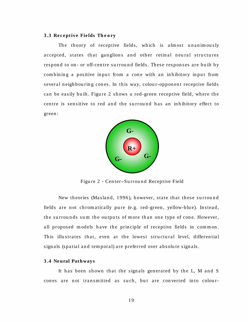
3.3 Receptive Fields Theory

The theory of receptive fields, which is almost unanimously

accepted, states that ganglions and other retinal neural structures

respond to on- or off-centre surround fields. These responses are built by

combining a positive input from a cone with an inhibitory input from

several neighbouring cones. In this way, colour-opponent receptive fields

can be easily built. Figure 2 shows a red-green receptive field, where the

centre is sensitive to red and the surround has an inhibitory effect to

green:

Figure 2 - Center–Surround Receptive Field

New theories (Masland, 1996), however, state that these surround

fields are not chromatically pure (e.g. red-green, yellow-blue). Instead,

the surrounds sum the outputs of more than one type of cone. However,

all proposed models have the principle of receptive fields in common.

This illustrates that, even at the lowest structural level, differential

signals (spatial and temporal) are preferred over absolute signals.

3.4 Neural Pathways

It has been shown that the signals generated by the L, M and S

cones are not transmitted as such, but are converted into colour-

R+

G- G-

G-

20

opponent signals. There is an achromatic signal, composed by L+M+S, a

red-green signal L-M+S and a blue-yellow signal L+M-S. This conversion

decorrelates the signals, thus allowing a more efficient transmission. The

place where these signals are generated is still under scrutiny4, but the

important part is that the L, M and S signals are decorrelated before

being transmitted to the higher levels of the visual system.

Depending on their center and surround functions, ganglion cells

exhibit band-pass activations, their contrast sensitivity reaching a

maximum for a certain peak frequency. For a constant signal (over their

receptive fields), these ganglions will not fire. The permanent vibration of

the eyes (independent of the conscious eye movements) assures a spatio-

temporal variation in the visual field; if the eye would stand still, a static

image would be invisible. This also explains why the blood vessels and

retinal neurons are not visible: since they do not move relative to the

retina, their shadow on the photoreceptors is invisible.

This illustrates an important aspect of the visual system: the

information is encoded with respect to contrast instead of absolute

values. One consequence is that it increases the dynamic range of the

visual system. Overall, the total dynamic range is about 10 orders of

magnitude (10 log10 units), of which the pupil dilatation and constriction

contributes with less than 1 log10 unit. In most viewing contexts, the

range of contrasts is less then 2 orders of magnitude, so the 10 orders of

magnitude can not be perceived simultaneously.

The relationship between the contrast sensitivity and the mean

luminance level was determined by Weber. Based on measurements,

4 see (Masland, 1996) for a discussion on this topic

21

Weber’s law states that the threshold intensity is proportional to the

background intensity. This change of the visual system relative to the

mean background signal is called visual adaptation.

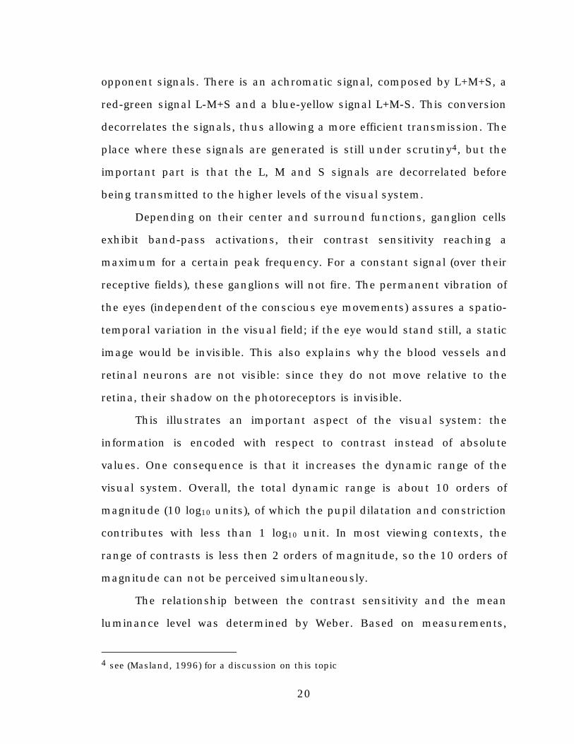
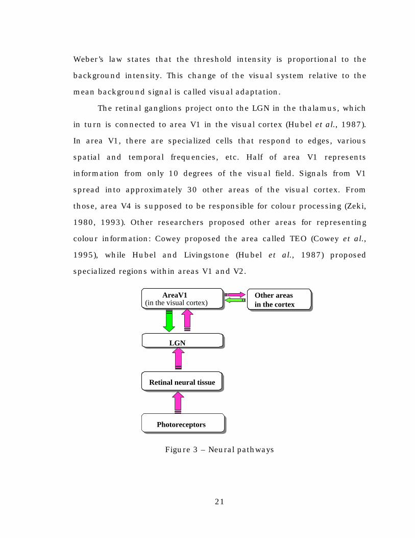
The retinal ganglions project onto the LGN in the thalamus, which

in turn is connected to area V1 in the visual cortex (Hubel et al., 1987).

In area V1, there are specialized cells that respond to edges, various

spatial and temporal frequencies, etc. Half of area V1 represents

information from only 10 degrees of the visual field. Signals from V1

spread into approximately 30 other areas of the visual cortex. From

those, area V4 is supposed to be responsible for colour processing (Zeki,

1980, 1993). Other researchers proposed other areas for representing

colour information: Cowey proposed the area called TEO (Cowey et al.,

1995), while Hubel and Livingstone (Hubel et al., 1987) proposed

specialized regions within areas V1 and V2.

Figure 3 – Neural pathways

Photoreceptors

Retinal neural tissue

LGN

AreaV1 AreaV1 (in the visual cortex)

Other areas in the cortex

22

As Wandell noted (Wandell et al., in press), most theories of vision

hypothesize that “there is a direct correlation between the segregation of

function at the neural level and the segregation of perceptual attributes.”

Since we can perceive colour as an attribute that is dissociated from

other visual attributes (which, in my opinion, does not mean that colour

is necessarily independent of other visual attributes), there must also be

a specialized neural structure responsible for colour representation.

3.5 The Neuron Doctrine versus Distributed Processing Models

The assertion that the receptive field of neurons describes the

representation generated by the activation of that neuron is at the heart

of the neuron doctrine. In this view (Hubel and Wiesel, 1977; Zeki, 1980,

1993), there are specialized neurons (or groups of neurons) that are

responsible for representations of shape and colour. This theory is

supported by neuroimaging data, which measures the correlation

between different perceptual features and the activations of some parts of

the visual cortex. It is also supported by experiments done on people

with visual deficiencies, such as dyschromatopsia (colour perception

loss).

An alternative hypothesis is that of distributed processing models,

which asserts that the processing of perceptual features is distributed,

and, therefore, there are no individual neurons that can be held

responsible for a certain representation. Since the processing is

distributed, it is impossible at this moment to support this doctrine with

experimental data.

Wandell (Wandell et al., in press) argues that the perceptual basis

for the functional segregation is only partially true, since there are some

23

perceptual representations that can not be segregated, because they are

coupled. Instead, he proposes an alternative theory that tries to reconcile

the two doctrines into a new framework. He asserts that the neural

diversity represents a “computational diversity rather than functional

specialization associated with perceptual attributes.” In this framework,

cortical lesions are not interpreted as damage to representational

structures but as disruptions in the information processing associated

with those representations.

Thus, the question shifts from “Where is this representation

located?” (colour, for example) to “How is this representation processed?”.

Wandell developed methods for computational neuroimaging in support

of his theory. Through functional magnetic resonance imaging (fMRI) he

traces the distribution of the cortical colour representation in different

areas of the visual cortex.

Although the anatomy and physiology of the visual system is still

under scrutiny, and many problems are still open, researchers have tried

to create models of the visual system since the beginning of the century,

long before the advances in neuro-physiological research. These models

were based mainly on psycho-physical experiments and form the core of

colorimetry, which will be discussed in the next chapter.

24

Chapter 4

Colorimetry and Colour Spaces

4.1 About Colorimetry

It is common knowledge that some objects appear different under

different illuminations. Moreover, there are objects that look alike under

some illuminants, but not when viewed under others. Thus, measuring

the conditions under which two objects look alike, as well as colour

differences between objects or between viewing conditions became an

important issue.

Colorimetry deals with the measurement of colour and colour

matches, as observed by an average observer with normal colour vision.

Of course, the methods of colorimetry can be extended to cover people

who have colour vision deficiencies, such as dichromats (observers with

only two types of cones) and anomalous observers (observers with three

types of cones, but which are different than the common cones). A lot of

research (Walraven et al., 1997) is done in the area of accommodating

displays and other colour devices with people with colour deficiencies.

To understand the way colorimetry works, it is important to

understand how the image is formed. Newton was the first to discover

the spectral nature of the light, when he decomposed daylight into its

components with the help of a prism. We can fully describe each source

of light by its spectral power distribution, i.e. the power emitted on each

wavelength. Each surface is also characterized by its reflectance spectral

distribution, i.e. the ratio of reflected light and incident light over all

wavelengths. The reflectance is a function ranging from 0 to 1 over the

25

considered wavelengths. However, fluorescent materials absorb the

incident energy at some frequencies and re-emit them at different, lower,

frequencies, in which case the reflectance function can be supra unitary

for some frequencies. It is important to notice that while for non-

fluorescent materials, their reflectance functions are independent of the

illumination, for fluorescent materials, their reflectance function depends

on the illumination, which makes them hard to measure.

In order to provide standardized viewing conditions, CIE adopted a

number of standard illuminants, such as D65, A or D50. These

illuminants model various daylights, tungsten lights, etc.

The Munsell chip set was created as one of the standards for

surface reflectances. They cover all colours that can be perceived by

human observers. The patches differ not only in hue, but also in

brightness and saturation. These chips have smooth reflectance

functions, such that they would look alike for observers who have small

discrepancies in their colour vision.

The third important factor in image forming is the human receptor

system. At photopic light levels, the cone responses are composed by

integrating, over all visible wavelengths λ, the illuminant in the scene I(λ)

with the reflectance R(λ) of the examined sample and with each of the

three cone sensitivity functions ρL(λ), ρM(λ), ρS(λ). Thus, we obtain three

values (L, M and S) that correspond to a surface viewed under a specific

illuminant. This process is called tristimulus integration.

26

=

=

=

∫∫∫

λ

λ

λ

λλρλλ

λλρλλ

λλρλλ

d)()(R)(IS

d)()(R)(IM

d)()(R)(IL

S

M

L

(2)

From the colorimetrical point of view, two coloured samples will

match only if their perceived value on each of the three colour channels

is equal. By integrating the illuminant with the reflectance and the

sensitivity functions of the cones, we reduce visual stimulus to a three

dimensional colour space. A consequence is that humans cannot

discriminate between different spectral power distributions and two

colour signals might match even if they are physically different. This

phenomenon is called metamerism.

From the description above, it might seem paramount to know the

exact sensitivity curves of the human cones in order to perform colour

matching and other colour measurements. However, it is not necessary

to know these functions exactly; a linear combination of them is enough,

because they provide equivalent matches (although the computed LMS

responses will be different for each set of sensitivity functions).

4.2 Colour Matching Functions

Colour-matching experiments are done by having an observer

tuning the brightness of three primary lights in order to match a test

light. Usually, this is done in a bipartite field, one side having the test

light and the other the projection of the three primary lights. The primary

lights are chosen such that they can cover the whole visible spectrum

27

and are linearly independent; they are usually red, green and blue in

appearance. During colour-matching experiments, it has been noticed

that colour matching is homogenous (if t matches c·p then a·t matches

a·c·p, where p is the primaries array, t the test light and a and c are

constants) and additive (if t matches e and t’ matches e’ than t+t’

matches e+e’). These linear properties are called Grassmann’s laws.

Based on the principles described above, one can determine a set

of colour matching functions that are within a linear transformation of

the human cone sensitivities. Given a set of test lights, the observer tries

to match them by scaling the three primaries:

t=c1·p1+c2·p2+c3·p3 (3)

Sometimes, if there is no combination of the primaries that can

match a test light, it is necessary to add a primary light to the test light

in order to do the match, in which case the corresponding constant is

negative:

t+c1·p1=c2·p2+c3·p3 (4)

is equivalent to:

t= -c1·p1+c2·p2+c3·p3 (5)

By choosing different primaries, we obtain different colour-

matching functions, but all will be within a linear transformation. CIE

defined a set of tristimulus functions, called CIE RGB, based on three

monochromatic primaries. These functions have some negative values. It

must be noticed that the CIE RGB tristimulus values that result from

integrating a colour signal with these sensor functions are different than

28

the RGB values in digital images, because the sensors used for digital

cameras are different.

4.3 The CIE 1931 Tristimulus Colour Space

In 1931, CIE defined a standard set of colour-matching functions,

called CIE XYZ tristimulus functions for the standard colorimetric

observer. These functions have been computed from experiments done

on a 2 degree visual field. They have only positive values (this aspect is

not important anymore, but at that time it simplified computations) and

Y corresponds to the brightness (more rigorously, to the photopic

luminous efficiency function, defined by CIE in 1924).

The primaries that generated the XYZ tristimulus functions are not

physically realisable, but the XYZ tristimulus functions are still within a

linear transformation from the human cones’ sensitivities. Because of

that, any two colours that generate the same cone responses will also

generate equal tri-stimulus values, thus preserving colour matching

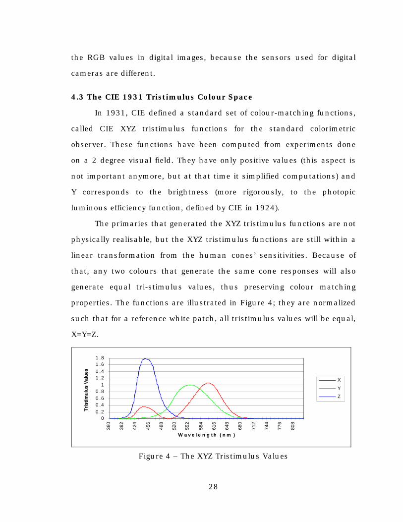
properties. The functions are illustrated in Figure 4; they are normalized

such that for a reference white patch, all tristimulus values will be equal,

X=Y=Z.

Figure 4 – The XYZ Tristimulus Values

00 .20 .40 .60 .8

11 .21 .41 .61 .8

360

392

424

456

488

520

552

584

616

648

680

712

744

776

808

W a v e le n g t h ( n m )

Tris

timul

us V

alue

s

X

Y

Z

29

4.4 CIELAB and other Colour Spaces

In practice, the XYZ colour space (as defined by the XYZ

tristimulus functions) is good for predicting colour matches, but the

colour differences in this space are not perceptually uniform. This is why

CIE adopted in 1976 two new uniform colour spaces, called CIELAB (CIE

L*a*b*) and CIELUV (CIE L*u*v*).

The CIELAB coordinates are computed form the XYZ tristimulus

values, using the following formulae (valid for normalized values greater

than 0.0088856):

L*=116(Y/Yn)1/3-16 (6)

a*=500[(X/Xn)1/3- (Y/Yn)1/3] (7)

b*=200[(Y/Yn)1/3 - (Z/Zn)1/3] (8)

The tristimulus values are normalized relative to the tristimulus

values of a white reference (Xn, Yn, Zn); this normalization is similar to

the von Kries adaptation model (as noted by Fairchild) and also

corresponds to the definition of colour given by Petrov (Petrov, 1993),

discussed earlier.

The L* coordinate is correlated with light-dark appearance, while

a* and b* correspond to the red-green and yellow-blue coordinates. It is

interesting that this perceptually uniform space is consistent with the

opponent colour theory of visual signal processing.

The Euclidean distance between two points in this colour space is

taken as a measure of colour difference.

30

Although CIELAB is a well established colour space, it has its

limitations. It has some problems predicting hue and it implicitly

includes an adaptation transformation, similar to van Kries, which in

some cases is not very accurate5.

The CIELUV space, on the other hand, includes a colour shift

(Judd adaptation model) instead of a von Kries adaptation for its white

normalization. This approach sometimes shifts colours out of their

physically realizable gamut. The equations are shown below:

L*=116(Y/Yn)1/3-16 (9)

u*=13L*(u’-u’n) (10)

v*=13L*(v’-v’n) (11)

where v’n and u’n are the chromaticity coordinates of the reference

white. v’ and u’ are coordinates in the following (almost uniform)

chromaticity space:

Z3Y15XX4

'u++

= (12)

Z3Y15XY9

'v++

= (13)

Recently, CIE adopted the CIECAM97s colour appearance model

(Luo et al., 1998), which improves on the CIELAB model. However, since

the experiments presented in the present thesis were performed in part

5 The shortcomings of the von Kries adaptation method will be discussed later in aseparate section.

31

before the adoption of this new standard, and since CIELAB provides a

good framework for reporting errors in a perceptual uniform space, we

did not use CIECAM97s or any of its revised proposals (Li et al., 1999).

4.5 Chromaticity Colour Spaces

In many cases, like colour correction, estimating the brightness of

the illuminant is not as important as estimating its chromaticity. This is

why it is sometimes more convenient to work in colour spaces in which

the brightness information has been eliminated. In CIELAB for example,

if we consider constant lightness, and work only in the a* and b*

coordinates, we have a two dimensional chromaticity space which spans

the red-green and blue-yellow coordinates of equal lightness (L is

constant).

The general idea is to normalize to only two coordinates, such that

the third one can be recovered from the other two. For example, given a

set of XYZ tristimulus values, we can convert them into an xy

chromaticity space, using the following equations:

ZYXX

x++

= (14)

ZYXY

y++

= (15)

The z coordinate is simply z=1-x-y; this approach normalizes all

components to the sum equal to 1, which is equivalent to a one-point

perspective projection onto the unit plane.

32

Other chromaticity spaces are built using projection rules like

x=X/Z and y=Y/Z. This projection space, although unbounded, has the

advantage that it is diagonal (Finlayson et al., 1994; Finlayson, 1995). In

diagonal spaces, sensor responses corresponding to the same surface

viewed under two different illuminants are within a diagonal

transformation.

4.6 Transformations in Colour Spaces

Transformations between different colour spaces occur whenever

we map colour spaces of different media into each other. Consider the

RGB colour space commonly used for representing colours in digital

images. Depending on the device6 used for displaying them (printer,

monitor, etc.), these images can have different colour appearances. For

example, to predict the appearance of a colour image on a monitor, one

must know the spectra of the phosphors, the gamma value of the

monitor and other parameters. Predicting the colour appearance of a

digital image over different media is a complicated problem, since each

device has its own calibration model and its own typical colour gamut

(i.e. the set of all possible colours it can produce) and these gamuts do

not necessarily coincide. Thus, a colour displayed on one device, might

not look the same when displayed on another device. Even more critical

problems can appear for highly saturated colours that can not be

represented at all on some devices. Usually, this problem of gamut

mapping is solved by minimising the perceptual errors that result when

mapping colours from one gamut to the other (Morovic et al., 1997).

6 ‘device’ is used in the sense of instantiating a type of media.

33

In what follows, I will not address the type of transformations that

are related to colour spaces belonging to different imaging devices, but

instead I will discuss transformations in the same theoretical colour

spaces. These transformations can serve as models of colour adaptation

for colour vision. Consider a diagonal model of adaptation of the following

form:

=

′′′

BGR

k000k000k

BGR

B

G

R (16)

and the corresponding chromaticity diagonal transformation:

=

′′

gr

c00c

gr

g

r (17)

If a projection of a diagonal transformation into a chromaticity

space is still diagonal, then the chromaticity space is said to be diagonal.

For example, if r=R/B and g=G/B, then we can write the diagonal

adaptation rule as:

=

=

′′

gr

c00c

BGBR

kk00kk

gr

g

r

BG

BR (18)

Diagonal spaces are important for colour constancy algorithms,

and their importance will be addressed when discussing those

algorithms.

4.7 Limitations of Color imetry

Colorimetry provides a set of tools and methods for determining

colour matches and computing colour differences. However, colorimetry

34

fails to predict colour appearance for complex scenes, where appearance

is modified by the interaction between the colours in the scene. Many

experiments (Land, 1977) show that the absolute values of the photo-

pigment absorptions do not explain colour appearance (absolute rates

can be assimilated to what a digital camera perceives and are highly

correlated to the surface reflectances). It is their relative rates that are

important for colour appearance and for providing colour constant

descriptors. We perceive the appearance of an object by the object’s

properties relative to the other objects in the scene and not only by the

amount of the light that it reflects, nor by the light’s spectral

distribution.

Moreover, colorimetry can not deal with colour constancy

phenomena, such as discounting the illuminant or estimating it, or

mapping a scene from one illuminant to another.

35

Chapter 5

Colour Constancy Algorithms

5.1 Introduction to Colour Constancy Algorithms

Colour constancy will be discussed in the context defined by Brill

and West (Brill et al., 1986), as “a subject’s ability to recognize object

colours in a fixed reflectance context independent of the illumination.” In

this framework, colour constancy algorithms deal with changes in

illuminants for a given scene, but do not take into consideration aspects

of colour appearance determined by the scene’s composition.

The goal of colour constancy algorithms is to provide colour

constant descriptors for the objects in a scene. There are two main

categories of colour constancy algorithms. One type of algorithm

estimates the illuminant and then corrects the given image relative to a

canonical illuminant. This is a practical approach to colour correction

and is closely related to imaging technologies. However, these algorithms

not only have to determine the illuminant, but also have to solve the

problem of colour correction (converting the image from one illuminant to

the other), which can be an important source of error for colour

appearance.

The other type of algorithm discounts the illuminant in a scene

and computes colour constant descriptors for the object in that scene;

these descriptors are the same for a given scene, independent of the

illuminant under which it was taken. These algorithms are better suited

for colour based object recognition because they implicitly provide

illuminant independent colour descriptions.

36

5.2 The Pros and Cons o f the von Kries rule

In 1902, Johannes von Kries proposed an adaptation model (von

Kries, 1902) that is still at the core of many of today’s colour constancy

algorithms. His adaptation rule states that the spectral sensitivity

functions of the eye are invariant and independent of each other, and

that the adaptation of the visual system to different illuminants is done

by adjusting three gain coefficients associated with each of the colour

channels.

The most common interpretation of his rule is that the coefficients

kL, kM and kS are adjusted such that a reference white surface would

have a constant appearance. L’, M’ and S’ are the adapted stimuli:

=

′′′

SML

k000k000k

SML

S

M

L(19)

The coefficients are adjusted relative to a reference white surface,

such that for that surface, the stimuli are constant, and equal to one:

kL=1/Lwhite ; kM=1/Mwhite and kS=1/Swhite (20)

This adaptation model is based on knowing the appearance of a

reference white surface in order to adapt the visual stimuli in a scene.

The colour of a reference white patch can also be interpreted as the

colour of the illuminant. Based on this model, many colour constancy

algorithms estimate the stimuli corresponding to a white surface in a

scene and then use the von Kries adaptation rule to colour correct the

image.

37

Worthey and Brill (1986) discussed the limitations of von Kries

adaptation rule and asserted the conditions under which the rule would

hold. They proposed three hypothetical retinas and described how the

von Kries adaptation rule would work with each of them. The first retina,

HR-1, consists of three narrow-band receptors, at three wavelengths, λR,

λG and λB. Because the receptors are narrow and do not overlap, the von

Kries rule would work perfectly with this type of retina.

The second type of retina, HR-2, consists of a single, broad-band,

receptor type, similar to the photopic efficiency function. This type of

retina illustrates the problem of metamerism, since many different

spectral reflectances map into the same stimulus value. A very good

analogy is that with a black and white image, where shades of blue are

perceived the same way as shades of red, for example. It is obvious the

von Kries rule would not work for such a retina, but the authors

included it in their study to show that broad sensors are a cause for

metamerism, which is a problem for colour constancy and for colour

adaptation models.

The third type of retina, HR-3, has three receptor types that are

broad but do not overlap, being similar to those used for digital cameras.

Because the sensors are broad-band, metamerism is still a problem.

However, it is possible to design an environment in which metamerism

does not occur: this is done by using three narrow-band light sources of

wavelengths that correspond to the peaks of the three sensors. Since

reflectances are sampled only at those wavelengths, the fact that the

sensors are broad-band does not induce metameric phenomena.

The problem is that the spectral sensitivities of human

photoreceptors are overlapping. Even in the case of a narrow-band light

38

source, which eliminates metamerism, it will activate more than one

receptor type. The adaptation matrix is non-diagonal in this case and the

more the sensors overlap, the larger the relative values of the non-

diagonal values.

To overcome this problem, Finlayson et al. (Finlayson et al., 1994a)

propose a sensor transformation called spectral sharpening. This

transformation converts any set of sensor sensitivity functions into a new

set of sensitivity functions that optimizes the von Kries adaptation model

by minimising the non-diagonal elements of the transformation matrix.

Thus, the adaptation rule p’=D·p, where p is the sensor response,

p’ the adapted responses and D the diagonal adaptation matrix, becomes

T·p’=D·T·p, where T is the sharpening transformation matrix. Sensor

based sharpening finds the most narrow-band sensors that are within a

linear transformation from the original ones. This sharpening is only a

function of the sensor sensitivity functions. For any given set of

illuminants and reflectance functions, a data-based sharpening will find

the optimal sharpening transformation for that database. The authors

have shown that for low-dimensional illuminant and reflectance

functions, spectral sharpening can eliminate the non-diagonal

components of the adaptation matrix. Thus, it assures that there exists a

diagonal transformation matrix (von Kries adaptation), which achieves

perfect colour constancy.

Experiments show that the sharpened sensors obtained through

different methods are similar and that they do not vary significantly with

the illuminants being used.

The conclusion that can be drawn (Finlayson et al., 1994) is that,

using sharpened sensors, a von Kries adaptation rule (a diagonal

39

transformation matrix) is a good enough model for colour constancy. The

only open problem is finding the reference white in a scene or estimating

its sensor responses, if not present in the scene. This approach is the

starting point of most colour constancy algorithms that are based on the

von Kries adaptation rule.

5.3 The Retinex Theory of Colour Vision

One of the most famous theories of colour constancy is Land’s

Retinex theory. The term ‘Retinex’ is derived from ‘retina’ and ‘cortex’ and

describes the biological mechanisms that convert luminous flux into

patterns of lightness.

This theory relies on experiments (Land, 1977) that confirm that

the visual system processes the light flux (i.e. colour signal) into

lightness values that are independent of the incoming flux. Colour-

matching experiments show that the lightness information is collected

and processed independently by each of the three retinex systems that

correspond to the photoreceptor classes. The perceived colours are the

result of the specific values of the three lightnesses. This implies that

colours are perceptual attributes of ratios instead of absolute values.

Thus, there is a much stronger correlation7 between the perceived

colours and the lightness values produced by the retinex systems than

between the perceived colours and the incident colour signals, which are

the product between the ambient illumination and the spectral

reflectance function of the viewed surfaces.

7 Since the experiments do not prove perfect human colour constancy, I use the term of‘correlation’ instead of stating an equivalence between the responses of the retinexsystems and perceived colours.

40

This theory, supported by experiments (Land, 1977) explicitly

states that there is no averaging between the values of the three retinex

systems and that the composition of the scene (in terms of average

reflectances) has no influence on the colour appearance predicted by this

theory. These results were challenged by Brainard and Wandell in a

paper (Brainard et al., 1986) that will be discussed later.

Land found a strong correlation between colour sensations and the

scaled integrated reflectances. Integrated reflectances are percentage

values, equal to the ratio between the integrated radiance of the

examined sample and the integrated radiance of a reference white.

Integrated radiances are the responses of the cone sensors to colour

signals (i.e. the integrated product of cone sensitivity functions and the

colour signal over the visible wavelengths). The scaled integrated

reflectances are obtained by scaling the integrated reflectances such that

they are equally spaced with the lightness sensations. It must be

noticed8, however, that this correlation is not perfect, resulting in

imperfect colour constancy results.

Based on these findings, Land developed several variants of

Retinex colour constancy algorithms. The goal of all these algorithms is

to derive the lightness information that corresponds to the reflectances of

the objects in the image, for each retinex class. This is done for each

photoreceptor class separately, but in the same way. After computing the

lightness information, the next step performed by the algorithms is to

find the area of maximum reflectance and determine if it corresponds to

a white patch or to some other colour.

8 see the correlation graph in Land’s paper (Land, 1977), page 118.

41

In the version published in (Land, 1977), the lightness information

is estimated by computing a series of random paths in the image. For

each path, the algorithm computes sequential ratios between values at

adjacent points. Changes above a certain threshold are regarded as

changes in reflectances; if the changes are smaller than the threshold,

the current ratio is set to one. Each time the current ratio is larger than

one, the whole path is reset, such that the area with highest ratio is

equal to one and all other compounded ratios are sub-unitary. In this

way, changes due to variations in illumination (which are considered to

be smooth, below the threshold) are discounted. After computing many

paths, the responses for each area are averaged and the results

designate the lightness values corresponding to those areas. This

computation is repeated over all three colour channels and the resulting

triplets of lightness (for each area) correspond to the perceived sensation

of colour. The sensation of white is generated by an area which has the

highest lightness on all three channels. However, the algorithm works

even if there is no white area in the image.

The Retinex algorithm is similar to a von Kries adaptation rule in

that the adaptation is done independently for each photoreceptor class.

This means that the limitations inherent to von Kries rule are also

present in the Retinex theory.

Other variants of the algorithm (Land, 1986) compute the lightness

values from the logarithm values of the sensor responses. Thus, the

computation uses differences of logarithm units instead of ratios of linear

units, but this does not change the performance of the algorithm

(Brainard et al., 1986).

42

Brainard and Wandell (Brainard et al., 1986) take a critical view at

the Retinex algorithm–the version published in (Land, 1986)–and discuss

its properties and limitations. They model the stochastic approach of

choosing the paths in the image through Markov chains and come to the

conclusion that the lightness value on channel k for an area x can be

computed as:

=

K

xkx

k GlogL

ρ(21)

where L is the lightness value, ρ is the photoreceptor response at

location x and Gk is the geometric mean of receptor responses from all

pixels in this image. This formula is valid for long path lengths, because

in that case the contribution of pixels is independent of their distance to

the pixel at location x. Another condition is that the number of paths

should be large, too.

For shorter paths, neighbouring pixels contribute more9 than

distant ones; for example, for a path length of 25, the neighbours of a

pixel contribute 6 times more than distant ones, while for a path length

of 200, the contribution is only of 1.25 times.

Since the lightness information is a function of the geometric mean

of sensor responses, Brainard and Wandell addressed the issue of

dependence of colour values on the scene composition. They used four

3-by-3 mondrians10 uniformly illuminated by CIE standard daylight D65.

9 This happens because neighbouring pixels are more likely to be included in a paththan more distant ones.10 Each mondrian is composed by three rows of three surfaces taken from the Munsellchip set.

43

The mondrians had the upper 2 rows identical and the lower row

contained 3 surfaces of the same hue, but different brightness and

saturation. This changes the geometric mean of the sensor responses for

each mondrian. The results of the experiment show that while that for

human observers the first two rows remain virtually unchanged, the

Retinex algorithm predicts different colours. Choosing shorter path

lengths did not improve the performance of the algorithm. The authors

drew the conclusion that the Retinex algorithm performs a normalization

that depends strongly on the surfaces in the image and thus is not a

good model for human colour constancy.

For long paths, the Retinex algorithm is similar to a von Kries

adaptation, where the diagonal entries of the adaptation matrix are equal

to 1/Gk. Another source of errors for the Retinex algorithm is the fact

that the photoreceptor sensors are broad and overlapping, which makes

the transformation matrix non-diagonal. A way to overcome this problem

is to use sharpened sensors (Finlayson et al., 1994a).

5.4 The Grey World

The grey world model takes a different approach to colour

constancy, by comparing the average content of a scene with some

expected values. This model assumes that the average of the perceived

world is grey and that any departure from this average is caused by a

shift in the illuminant’s colour. Some versions of the algorithm scale the

sensor responses such that the average is back to grey, the illuminant

being discounted and colour-constant descriptors are obtained for all

colours in the scene. There is a certain resemblance with the logarithmic

44

version of the Retinex algorithm, where in the case of long path lengths,

a normalisation relative to the geometric average was performed, as

shown in (Brainard et al., 1986).

The origin of the grey world algorithm dates back to Helmholtz11,

who attributed the phenomenon of human colour constancy to the

discounting of the illuminant. This idea was continued by Helson12, who

assumed that colours are detected with respect to a single adaptation

level, which corresponds to an average grey. The average was computed

as a weighted function of the reflectances present in the visual field.

Judd13 considered that the average chromaticity of the reflected light is

equal to the chromaticity of the illuminant.

Buchsbaum (Buchsbaum, 1980) developed an extended model of

the grey world. He assumed that spectral reflectances and illuminants

can be modelled with only three basis functions (that span a non-

orthogonal colour space), discounting metamerism and other problems

that occur when using overlapping sensors. His model computes the

illuminant and the surface reflectances by matching them with linear

combinations of the basis functions.

Buchsbaum’s main assumptions are that (1) the entire scene can

be processed together, having a single reflectance vector (computed as a

weighted average over different areas of the scene), and that (2) the visual

system assumes a fixed internal standard reflectance vector for the

overall scene average.

11 see (Buchsbaum, 1980).12 ibid.13 ibid.

45

This means that the illuminant is estimated on the basis that it

acts on an average homogenous surface reflectance, which is assumed to

be the internal standard one. After computing the illuminant, all surfaces

are corrected accordingly.

In practice, it happens very often that the standard average

reflectance (whatever it might be) is not equal to the actual visual field

average, in which case the grey world algorithm yields poor results. This

algorithm has the tendency to shift surface colours towards grey,

desaturating them. Thus, an image containing only a blue sky will

become grey, because the algorithm will consider the average blue

reflectance as an effect of the illuminant and will correct the scene such

that the average becomes grey, equal to the internal one. Choosing an

internal bluish average would help for that particular scene, but would

yield large errors when correcting an image of a forest, where the average

is greenish. Moreover, choosing the weighting function that averages the

reflectances is another problem, since different functions will give

different results.

Gehrson et al. (Gehrson et al., 1988) improved on Buchsbaum’s

grey world algorithm by making some a priori assumptions about the

reflectances and illuminants, based on statistical measurement of

naturally occurring reflectances and illuminants14. They computed the

internal standard average reflectance from the set of 370 reflectances

determined by Krinov (Krinov, 1947). They also built a three dimensional

model for illuminants, based on the study done by Judd (Judd et al.,

14 Other algorithms that use statistical approaches will be described in the followingSections.

46

1964). and worked in the decorrelated space, defined by the finite

dimensional linear model in which illuminants and reflectances are

described in terms of weights of basis functions.

The image is segmented in a set of areas according to their

chromaticity. Then the average of these areas was again averaged to yield

the total average of the image reflectance. This averaging method has the

advantage that it represents all surfaces equally, independent of their

area.

This algorithm is still tributary to the idea of a fixed reference

average reflectance, although Gershon’s algorithm computes the

illuminant, based on some a priori knowledge about the world. However,

there are other colour constancy algorithms, based on linear models,

that are not dependent on any fixed reference value. Such a linear model

will be presented below in section 5.5.

John McCann (McCann, 1997) performed a series of experiments

which proved that the human visual system does not achieve colour

constancy based on the average ‘quanta catch’ (i.e. the averaged

tristimulus values), even in the case of local surrounds. As a

consequence, he states that colour constancy must be based on a

normalisation process, similar to the Retinex algorithm.

5.5 Finite Dimensional Linear Models

Finite dimensional linear models are used to impose certain

restrictions on the illuminants and reflectances in order to make the

recovery presented above possible. One of these models was proposed by

Maloney and Wandell (Maloney et al., 1986; Wandell, 1987).

47

In the definition of the colour signal:

( ) ( ) ( )λλλ SEC = (22)

where E(λ) is the spectral power distribution of the illuminant and S(λ) is

the spectral reflectance function of a surface, the product is

commutative, so it is impossible to recover uniquely the surface and

illuminant spectral functions, even if we can measure the colour signal

over all wavelengths. The recovery is even more difficult (assuming that

we can separate E(λ) and S(λ) in the colour signal) when we only have the

responses ρ of the sensors, which are the integrated products of the

colour signal C(λ) and the sensor sensitivity functions R(λ):

( ) ( )∫=λ

λλλρ dRC (23)

over all visible wavelengths λ, where R(λ)>0.

Without some assumptions, it is impossible to recover both E(λ)

and S(λ) from arrays of only three numbers (i.e. the number of sensor

responses, usually equal to three).

The first assumption of the model (Wandell, 1987) is that the

illuminant varies smoothly over the visual field. In what follows, I will

discuss only the situation of a constant illuminant over the whole scene.

Local processing techniques15 can be applied to accommodate spatial

variations of the illuminant.

Assuming a linear model for the illuminant and for the

reflectances, we can write them as a sum of weighted basis functions:

15 The scene is processed in overlapping regions, with requirements of consistency atoverlapping points.

48

( ) ( )( )∑=

=ED

1iiiEE λελ and (24)

∑=

=)S(D

1ii

xi

x )(S)(S λσλ (25)

where Ei and Si are the sets of basis functions, D(E) and D(S) are

the dimensions of the spaces spanned by the basis functions (and equal

to the number of basis functions for each space), ε and σ are coefficients

(or weights) of the basis functions that uniquely determine the illuminant

and reflectances, and x designates a location in the scene. Each

illuminant is characterized by a set of D(E) coefficients{ε1, ..., εD(E)}. The

same applies to reflectances.

We can write the formula of sensor responses:

xE

x σρ Λ= (26)

where for the illuminant E, the sensor responses ρx in area x depend only

on the coefficients σx of the basis functions that determine the

reflectance function of area x. The kjth entry of the matrix ΛE is equal to:

( ) ( ) ( )nknjnj,k

E RSE λλλ∑=Λ (27)

The surface reflectance coefficients represent illuminant inde-

pendent colour descriptors of the surfaces in the scene. This is done by

computing the coefficients σ, as a function of known sensor responses ρ:

xE

x ρσ 1−Λ= (28)

49

Another necessary constraint is imposed on the dimensionality of

surface reflections: D(S) must be greater than the number of sensor

classes, otherwise the solution is underdetermined. Of course, if the

actual dimensionality of the reflectances in a scene is higher than the

constrained one, the model will have errors in estimating the colour-

constant descriptors.

Wandell noticed that this constraint forces the sensor responses to

lie in a hyper-plane in the sensor response space. The position of the

points in this plane is determined solely by σ, while the position of the

plane in the sensor space is determined by the illuminant E and its

coefficients ε. Based on this observation, Maloney developed a three step

algorithm:

The first step is to identify the hyper-plane that contains the

sensor responses. Once this hyper-plane is determined, it is used to

extract the lighting information ε, specific to the illuminant. The final

step is to compute the pseudo-inverse of the lighting matrix 1−ΛE , which

permits the computation of the colour-constant descriptors σ.

The dimensionality of the illumination space is also constrained,

and must be equal or less than the number of sensor classes.

Formally written, the algorithm works like this: consider ∆, the set

of sensor responses from the image. The vector π, perpendicular to the

hyper-plane formed by these responses can be computed from ∆π=0. In

order to obtain π, it is necessary that the number of sensor responses

included in ∆ be greater than D(E). In practice, a larger number will

reduce the effect of noise and will yield better results.

The second step takes advantage of the symmetry of illumination

and surfaces in their inner product, such that we can write:

50

εσρ Sx

Ex Λ=Λ= (29)

It follows that 0=Λ επ ST , so we can solve for ε : Πε=0. After we

compute ε, the lighting matrix ΛE becomes known and we can solve for

the colour-constant descriptors σ.

When the set of possible illuminants and reflectances is known,

the basis functions can be computed by principal component analysis in

order to minimise the correlation between dimensions.

Wandell obtained a good linear fit for the Munsell colour chips, but

this result should not be extrapolated, in my opinion, to other surface

reflectances. This is because the Munsell chip set was designed to have a

low dimensionality in order to accommodate observers with slightly

different cone sensitivities.

5.6 The Dichromatic Model and its Applications

Most models of reflection assume that the surfaces are

Lambertian, i.e. perfectly matte and appear equally bright from all

directions (isotropic). In practice however, materials are rather

inhomogeneous, being composed of a medium and a colorant, e.g.

plastics, paints. Depending on the viewing angle, they might appear more

or less glossy, which can not be explained by the Lambertian model.

The dichromatic model of reflection (Shafer, 1985) assumes that

materials are inhomogeneous. The incident light interacts first with the

interface of the material, causing an interface reflection. The interface

reflection is perceived as a highlight or specularity; this is why it is also

called specular reflection. The relative amount of reflected light as well as

the reflection angle are predicted by Fresnel’s laws. Since the index of

51

refraction is relatively constant16 over the visible spectrum, the interface

reflection is assumed to be constant with respect to the wavelength and

consequently to have the same spectral composition as the incident light.

The other part of the incident light, which was not reflected at the

interface, is scattered inside the body of the material (by the colorants

within) and is either absorbed, transmitted (if the material is not

opaque), or re-emitted through the interface. This produces a body

reflection, which is assumed to be isotropic and usually with a different

spectral composition than the incident light. The difference in spectral

composition is caused by the selective absorptions of the colorants over

the visible wavelengths. Fluorescent materials re-emit the light at

different wavelengths, and they will not be addressed by this model.

The dichromatic model of reflection states that the total radiance of

reflected light is equal to the sum of the radiance of the interface

reflection and radiance of the body reflection. Moreover, the two

components are independent:

)(c)v(m)(c)v(m),v(L),v(L),v(L bbiibi λλλλλ +=+= (30)

They can be further decomposed into a magnitude function m(v),

which depends only on the viewing conditions v (incidence and phase

angle) and a composition function c(λ), which depends only on the

wavelength. A constraint imposed on the model is that the magnitude

functions are bounded 0<m<1.

16 within a few percent.

52

Due to the fact that the tristimulus integration is linear, we can

write the sensor responses as a sum of two components that correspond

to both types of reflection:

ρ=miρi+mbρb (31)

This implies that all sensor responses for the same surface will lie

in a parallelogram defined by ρi and ρb in the sensor response space. The

magnitude coefficients m determine the position inside this parallelogram

and correspond to the relative weights of each reflectance type.

For each surface, it is easy to compute the vectors ρi and ρb based

on a set of sensor responses that correspond to a single surface: given

the points, the first step is to fit a plane through these points and

through origin (this is equivalent to assuming that there is no diffuse

light in the scene). The second step is to fit a parallelogram to these

points in the plane. The sides of the parallelogram will be ρi and ρb. In

this way, one can determine the direction and implicitly the chromaticity

of the illuminant, just by examining the direction of ρi.

Lee (Lee, 1986) developed a simple method for estimating the

chromaticity of the illuminant, based solely on the specular reflections in

the scene. Chromaticity values of additive mixture of two colours, with

chromaticities (x1,y1) and (x2,y2), will lie on a straight line (in a

chromaticity space) connecting the points of the two colours, as shown in

Figure 5:

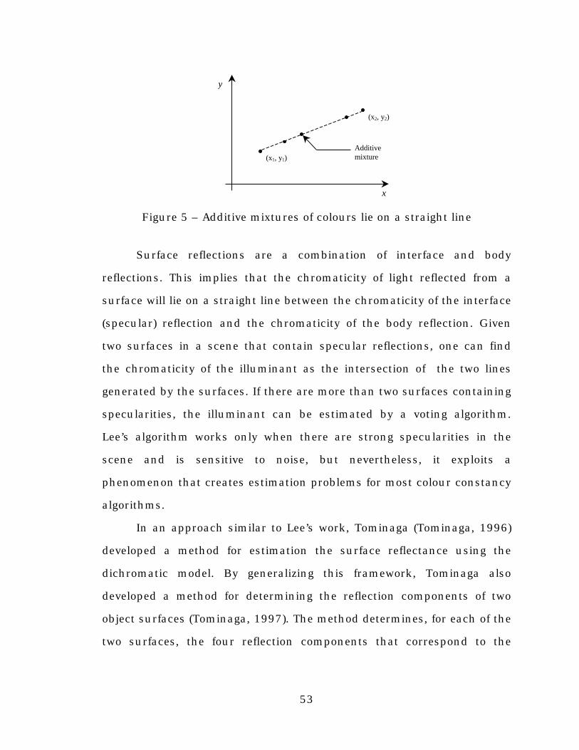
53

Figure 5 – Additive mixtures of colours lie on a straight line

Surface reflections are a combination of interface and body

reflections. This implies that the chromaticity of light reflected from a

surface will lie on a straight line between the chromaticity of the interface

(specular) reflection and the chromaticity of the body reflection. Given

two surfaces in a scene that contain specular reflections, one can find

the chromaticity of the illuminant as the intersection of the two lines

generated by the surfaces. If there are more than two surfaces containing

specularities, the illuminant can be estimated by a voting algorithm.

Lee’s algorithm works only when there are strong specularities in the

scene and is sensitive to noise, but nevertheless, it exploits a

phenomenon that creates estimation problems for most colour constancy

algorithms.

In an approach similar to Lee’s work, Tominaga (Tominaga, 1996)

developed a method for estimation the surface reflectance using the

dichromatic model. By generalizing this framework, Tominaga also

developed a method for determining the reflection components of two

object surfaces (Tominaga, 1997). The method determines, for each of the

two surfaces, the four reflection components that correspond to the

(x1, y1)

(x2, y2)

x

y

Additivemixture

54

illuminant colour, to the object colour and to the specular and body

interreflection colours.

Based on the dichromatic model of reflection, Finlayson and

Schaefer (Finlayson et al., 1999) developed an algorithm that uses only

one surface (containing specularities), and hence only one dichromatic

line. The illuminants are constrained on the Planckian locus. Thus, the

actual illuminant is located at the intersection of the Planckian locus

with the dichromatic line given by the surface’s specularities. In this way,

single surface colour constancy can be achieved.

5.7 Gamut Mapping Algorithms

Gamut mapping algorithms are based on the observation that the

nature of illuminants constrains the plausible set of sensor responses.

For instance, if the illuminant used in a scene is red, no surface can

have a very high response on the blue channel. Thus, each surface in the

scene introduces a new weak constraint on the colour of the illuminant

and by intersecting all these constraints, the algorithm determines a set

of plausible illuminants, from which it picks its best estimate.

The first gamut mapping algorithm was designed by Forsyth

(Forsyth, 1990). His model assumes that the scenes are composed of flat,

matte surfaces and that the scene is illuminated by only one uniform

illuminant. Another assumption concerns the set of possible illuminants,

which should be “reasonable” (i.e. they can be parameterized).

Central to the gamut mapping algorithm is the idea of a canonical

gamut. A gamut Γ is the (convex) set of the sensor responses to all

physically realisable surfaces, viewed under a certain illuminant. The

55

canonical gamut Γ(C) is the gamut taken under a standard, canonical

illuminant. In practice, this illuminant is taken such that the sensor

responses would be calibrated for that illuminant (i.e. a reference white

patch would produce equal responses for all sensors), but other

illuminants can be used instead. Any gamut is convex because a convex

combination of two surfaces would also belong to the gamut. If p1 and p2

are two surfaces that belong to the gamut, any convex combination

21 )1( ppp x αα −+= also belongs to the gamut because it is physically

realisable.

Consider a scene I under an unknown illuminant. For any surface

px, a diagonal transformation Dx, that maps px inside the canonical

gamut Γ(C) is a possible solution for the illuminant. Finding the set of all

possible mappings Dx is equivalent to mapping px to all points on the

convex hull H(C) of the canonical gamut.

The set ∆ of all possible mappings D that map simultaneously all

points of the scene I into the canonical gamut is the intersection of all

mappings Dx, for all surfaces px in the scene:

Ix

xD=∆ , ∀ px. (32)

Since diagonal transformations preserve the convexity of sets, this

is equivalent to computing the intersection of the diagonal mappings Dx

belonging to surfaces defining H(I), the convex hull of I:

Ix

xD=∆ , px∈H(I). (33)

56

After determining the set ∆ of all possible gamut mappings, the

algorithm selects the mapping that yields the gamut with the largest

volume. Finding the gamut with the largest volume is easy, because

diagonal transformations transform a volume (e.g. the original gamut)

into a volume (e.g. the map of the image gamut into the canonical gamut)

multiplied by the trace of the mapping matrix, so the map with the

largest trace will be the chosen one.

Forsyth’s algorithm performs well under controlled conditions, but

real images which usually contain specularities, curved surfaces, and

noise will degrade its performance. Another problem is that the algorithm

tries to recover not only the chromaticity of the illuminant, but also the

intensity. This will yield large errors if the image is not normalized. These

errors in intensity estimation can make an image look dark, or worse, it

can clip bright pixels in the image

Finlayson (Finlayson, 1995, 1996) improved Forsyth’s algorithm by

working in a chromaticity space instead of a three dimensional space and

by imposing certain restrictions on the illuminant. His method, called

‘colour in perspective’ (Finlayson, 1996) uses a perspective chromaticity

space: r=R/B and g=G/B, where R,G, and B are the sensor responses on

the three colour channels. This perspective space is also diagonal

(Finlayson, 1996) and it preserves the convexity of gamuts during

diagonal transformations. Working in 2D instead of 3D reduces the

computational complexity of the algorithm that performs the convex hull

intersections. Visualisation techniques are also easier to implement in

2D.

Finlayson added another constraint to the set of possible diagonal

gamut mappings, by defining an illumination gamut, composed of the set

57

of all plausible illuminants. A gamut mapping D, described above in

Forsyth’s algorithm, is considered possible if its inverse D-1 also maps the

canonical illuminant into the illumination gamut. As a consequence, the

set of all possible gamut mappings ∆ is intersected with the set of

mappings satisfying the illumination constraint.

Selecting a mapping is still a problem. One way is to pick the one

that yields the maximum area, in a similar mode as described in

Forsyth’s 3D algorithm. Choosing an average mapping is a different

solution, but both are inappropriate since the computations were done in

a perspective space, which is non-linear and distorts distances.

Finlayson et al. (Finlayson et al., 1997) propose a new approach to this

problem. They reconstruct the three dimensional mapping set by

converting the (r,g) coordinates of the hull of all possible gamut

mappings back into three dimensional (r,g,b=1) coordinates. These

points, which lie on a plane defined by b=1, are then connected to the

origin, thus forming a cone. The gamut mapping is selected as the mean

in the three dimensional space. Of course, since the intersections were

done in the perspective space, the gamut mapping will be recovered up to

a scaling factor. This mean, projected back into the projection

chromaticity space is different than the mean computed in the projection

space and it gives a more accurate estimate of the chromaticity of the

illuminant.

Barnard et al. (Barnard et al., 1997) addressed the problem of non-

uniform illumination within a scene, which introduces yet another

constraint in Finlayson’s algorithm. Different mappings are computed

locally, generating a relative illumination field. This relative field is used

to eliminate the change in illuminant across the scene and make the

58

scene look as if it were illuminated by the illuminant at an arbitrary

reference point. All relative illuminations must satisfy the constraints

imposed on the illumination, which further restricts the number of

possible solutions.

The gamut mapping algorithms are among the best performing

colour constancy algorithms to date.

5.8 Probabilistic colour constancy

Probabilistic colour constancy algorithms use stochastic models for

surfaces and illuminants to derive maximum likelihood estimates of the

scene’s illuminant. In a sense, they are a natural extension of

Buchsbaum’s grey world algorithm (Buchsbaum, 1980) in that they

exploit the information about the distribution of the surface reflectance

functions instead of only their spatial average over the entire scene. Prior

distributions of possible illuminants also help in estimating the

maximum likelihood chromaticity of the illuminant.

These stochastic algorithms can also be considered an extension of

the gamut mapping algorithms (Forsyth, 1990; Finlayson, 1995). Instead

of computing ‘strict’ intersections of transformations corresponding to

possible surfaces and illuminants, they derive ‘soft’ intersections of

probable surfaces and illuminants.

As with all algorithms that depend on a priori knowledge about the

world, their accuracy depends heavily on the composition of the

perceived scene, relative to the a priori distributions empirically

determined. Suppose that an image contains a set of n sensor responses

(RGBs), corresponding to n independent surfaces. Then, the likelihood

59

L(A), that the scene was taken under illuminant A(λ) is given by the joint

probability:

∏=

=n

1ii )A|RGB(p)A(L . (34)

The Bayesian colour constancy algorithm designed by Brainard

and Freeman (Brainard et al., 1997) extends finite-dimensional linear

models by using stochastic models of surface reflectances and illuminant

power distributions.

Suppose p(x) is a prior probability density function of the

parameters vector x, which characterises an event E. In our case, x will

correspond to parameters characterizing surface reflectance functions

and illuminant power distributions. In the case of finite-dimensional

linear models, only a few parameters are enough to model surfaces and

illuminants17. If y is the observed data, its likelihood is p(y|x) – the

conditional probability of y, given that x occurred.

Bayes’ theorem computes the posterior probability p(x|y). It is the

probability that the parameters x caused the observation y:

)y(p)x(p)x|y(p

)y|x(p = (35)

Given p(x), an a priori model for illuminants and surfaces, and y,

the observed scene, one can compute the probability of each vector x and

implicitly, the probability corresponding to each illuminant. To obtain a

single estimate of the illuminant from all possible ones, a loss function

17 see the discussion about linear models in section 4.4

60

L( x , x) needs to be introduced. The loss function specifies the penalty for

choosing an estimate x when the correct answer is x. If the loss function

is shift invariant, then it depends only on the difference x -x. Given a loss

function L and a posterior probability p(x|y), the goal is to minimise the

Bayesian expected loss:

dx)y|x(p)x,x(L)y|x(L

x∫= (36)

Usually, x is chosen such that it either maximises the posterior

distribution or it minimises the mean squared error of the distribution.

However, Brainard and Freeman introduced a new loss function, that is

more appropriate to perception. The local mass loss function rewards

approximately correct answers and penalizes all estimates that yield a

large error equally. This way, the algorithm finds “the most probable

approximately correct answer.”

Illuminants and surface reflectances were modelled using linear

models. The surface reflectances sj were modelled by a set of weights wj

and basis functions Bs, such that sj=Bswsj. Illuminants were modelled in

the same way: e=Bewe. Brainard and Freeman noticed that the weights

are not uniformly distributed, but have a normal probability density

function. If the illuminant and surfaces in a scene are independent, then

p(x)= p(ws,we)=p(ws)p(we).

Finalyson (Finalyson et al., 1997) extended his previous “Color in

Perspective” colour constancy algorithm (Finlayson, 1995) by using a

correlation matrix to establish a stochastic relationship between the

chromaticities in a scene and a set of illuminants. This matrix is used as

61

an associative memory to correlate the data from a scene with the set of

possible illuminants. The rows of the matrix correspond to all perceivable

chromaticities (empirically determined), while the columns correspond to

the set of possible illuminants. An element eij of this matrix is set to “1” if

the chromaticity i can be perceived under the illuminant j, and “0”

otherwise. This matrix is computed based on an a priori observation of

the world, i.e. based on a large reference set of surfaces and illuminants.

The illuminant of a scene is estimated by a simple voting scheme, that is

based on the chromaticities existent in the scene.

By using binary entries into the correlation matrix, it is implicitly

assumed that all illuminants and chromaticities are equally likely (they

have a uniform distribution). This algorithm can be further improved by

using knowledge about prior distributions for chromaticities and

illuminants. Thus, the elements eij of the correlation matrix will contain

the probability of illuminant j, given chromaticity i:

)i(p)j(p)j|i(p

)i|j(pe ij == (as stated by Bayes’ theorem) (37)

This method is simple and fast. However, as with all other

probabilistic approaches, it depends on prior knowledge about the world.

Another common feature of all probabilistic algorithms is that they

produce not only an estimation of the illuminant, but also provide an

estimation of the confidence in that illuminant. This is done by

comparing the likelihood value of the chosen illuminant with the

likelihood values of the other ones.

62

It is my opinion18 that, although probabilistic models provide a

good computational approach to colour constancy— especially when the

composition of the perceived scene corresponds to the prior knowledge

about the world— the human visual system uses a different approach to

obtain colour constant descriptors for the surfaces in a scene.

5.9 Neural Network Approaches to Colour Constancy

Previous neural network approaches to colour constancy used

neural networks either as implementations (in hardware or software) of

existing colour constancy algorithms, such as Retinex, or as emulations

of simplified models of the human (or primate) vision system. In both

cases, neural networks could not overcome the inherent theoretical

limitations of the algorithms they were implementing and therefore the

results (in terms of accuracy of the illuminant estimation) are modest

and do not solve the colour constancy problem.

Hurlbert and Poggio (Hurlbert et al., 1988; Hurlbert, 1991)

developed and tested a neural network based on a version of Land’s

Retinex algorithm. The authors assume a Mondrian world in which the

illuminant varies smoothly across the image, while surfaces have sharp

edges. The algorithm is based on the assumption that the image

irradiance can be written for each chromatic channel as the product of

the illumination intensity and surface reflectance S(x)=E(x)R(x), and by

taking the log, we obtain s(x)=e(x)+r(x), where s=log(S), e=log(E), r=log(R).

18 for experiments supporting my opinion, see (McCann, 1997).

63

Another assumption is that there exists a regularisation operator

L, which is linear and is of the following form:

Ls=r (38)

L is a matrix equal to L=rs+, where s+ is the Moore-Penrose pseudo-

inverse of r:

r+=rT(rrT)-1 (39)

L is computed by over-constraining the problem. L will recover r,

when a new vector s is input.

This algorithm is equivalent to discounting the variation of the

illuminant. Its Fourier analysis shows that it is a band-pass filter, which

cuts low frequencies determined by smooth changes in the illuminant

and high-frequency signals caused by noise.

The same algorithm was implemented with a linear neural

network, which was trained to perform a linear map between pairs of

images: input images, taken under a varying illuminant were mapped

into the same images where the illuminant was discounted. It has been

shown (Hertz et al., 1991) that a mathematical model of a linear neural

network that is trained by using a gradient descent algorithm is

equivalent to the pseudo-inverse that maps the network’s input space

into its output space.

In this context, of strong constraints imposed on the model, their

algorithm performs well at discounting the spatial variation of the

illuminant, but it does not solve the colour constancy problem better

than the Retinex algorithm, since it does not provide for a method of

scaling the three channels.

64

Moore et al. (Moore et al., 1991) also implemented the Retinex

algorithm using a VLSI analog neural network. This network is based on

Zeki’s findings (Zeki, 1980, 1993), that there are cells in the V4 area of

the visual cortex that respond to the perceived colour rather than to

specific frequencies. These cells have a typical centre-surround activation

pattern; if the surround has the same frequency as the centre, the cell

will not respond. The Retinex method they implemented involves

subtracting, for each point in the image, the log of the intensity in that

point from the log of a weighted average around that point. This method

is equivalent to a convolution which normalizes each point relative to a

local average.

However, due to the convolution process, there is an unwanted

artefact that appears at sharp edges: Mach bands. These bands are

caused by the colour induction that appears due to the surround local

processing. Moreover, due to the implicit grey world assumption, the

algorithm can easily fail. This is why Moore et al. introduce the notion of

edginess, which quantifies the magnitude of the spatial derivative. Its

value ranges from 0, for a homogenous local surround, to 1, for a region

with high-frequency responses (corresponding to sharp edges). The

output of a pixel is computed as a function of the centre (the value of the

pixel being considered), the surround, and the edginess:

output = centre - surround·edginess.

Thus, in smooth regions, the surround has no effect on the output,

which also reduces the effect of the grey world assumption. This

approach also eliminates much of the colour induction. For smooth

images, however, the output image will be similar with the input one, so

no colour correction will take place.

65

This neural network implementation, which is very simple,

consists of three resistive grids. It has the advantage that the processing

is carried in parallel, thus being much faster than the convolution

approach.

Usui (Usui et al., 1992) designed a neural network, shown in

Figure 6, that decorrelates the triplets of sensor responses, thus

obtaining colour constant descriptors in the decorrelated space. The

decorrelation is the result of a neural network with lateral asymmetric

feed-back connections and is similar to PCA (Principal Component

Analysis).

+1 Bias

b1

b2

b3

x1

x2

x3

z1

z2

z3

w11, 21,31

w22,32

w33

Figure 6 – Neural network with asymmetric feed-back connections

The input signal xi is added to a bias signal bi:

yi=xi+bI (40)

The output zi is determined by yi and the weighted sum of the

output of the other neurons:

∑>

+=ji

jijii zwyz (41)

In matrix form, this is equivalent to:

66

z=(x+b)+wz (42)

which is equivalent – after a transient phase – to:

z=(I-w)-1y=Ty (43)

The role of the bias is to transform the input into a zero-mean

signal. All weights are tuned according to an anti-Hebbian rule.

For training, the authors used a large set of Munsell chips and

three different illuminants. They trained three different networks, one for

each illuminant. The training starts from the same initial state, which is

defined as the state of the network after the completion of the training for

the first illuminant. In other words, the network is trained for one

illuminant and, after the learning process converges, different networks

are trained starting from this state. After training, the networks generate

almost the same output representations, for the same image taken

under the three different illuminants for which the network was trained.

In my opinion, this neural network does not exhibit any form of

colour constancy. In the first place, the authors use the correct network

for each of the scenes being tested, implying that they know the

illuminant in advance, i.e. the network trained for fluorescent light is

used for the scene taken under fluorescent light. Second, the fact that

the networks transform a scene taken under different illuminants into

the same decorrelated representation is due to the training algorithm,

which uses a decorrelating transformation (i.e. the first neural network)

as the starting point for the other transformations.

67

Based on the primate visual system, Courtney (Courtney et al.,

1995, 1995a) developed a multi-stage neural network that produces

colour constant descriptors. The network is composed of a number of

levels, each corresponding to a specific stage in the primate visual

system from the retina to the cortical area V4.

The first stage of the neural network converts the input image

(whose size is 27x27) into a matrix of cone RGB19 activation levels. The

image is artificially generated by integrating Munsell reflectances with a

set of illuminants. The neurons corresponding to the first layer of the

network have a Naka-Rushton response function:

xx

x

Q

QA

σ+= (44)

where A is the output of the cone, Qx is the activation (a weighted

sum of all R, G, or B values generated from the image), σ is a threshold

and x=0.7… 1.0.

For all other neurons (i.e. in the other layers) the activation

function is a sigmoid, with a gain factor β (to control the slope of the

linear portion) and scaling parameters (Min and Max):

Mine1

1)MinMax(A )Q( +

+−= −− σβ (45)

The next layer models the effect of spectral opponency. Each

neuron receives excitatory input from a single cone, which lies in the

centre of the receptive field, and inhibitory input from several cone types

19 I keep the notation used in both papers

68

that surround the centre. The weights of these surrounding neurons are

determined by the distance from the centre and decrease according to a

Gaussian attenuation function. The weights of different cone types in the

surround are not equal: for example, a centre-surround neuron, that is

activated in its centre by stimuli coming from an R cone, will have the

weights that connect the surround field to the G cones twice as large as

those that are connected to the R cones. In this way, two R and G centre-

surround cells that span the same field will not merely be opposed, but

will have linearly independent activations.

Neurons corresponding to B cones will receive inhibitory inputs

from their surround coming from equally weighted R and G cones. In this

way, three linearly independent combinations of the R, G and B cones

are generated. The centre-surround sensitivities are not equal, but are in

a ratio of 2:1.

The next layer corresponds to area V4. The neurons in this layer

have large inhibitory surrounds (“silent surrounds”) that have the same

frequency response (i.e. R, G or B) as the excitatory centre. These

neurons, which can be either on- or off-centre, receive activation only

from a single type of spectrally opponent neuron.

Reference neurons are also included in the network, to provide

only local colour information. The final output of the network is given by:

O=B+c1P+c2N , where B is the output from the reference cell,

P is the output from the on-centre neurons and N is the output from the

off-centre neurons.

69

The authors claim that the network exhibits colour constancy and

colour induction (simultaneous contrast), being in agreement with

psychophysical data of human colour constancy. Due to the local

reference neurons, the network also compensates for the loss in colour

contrast, caused by local averaging. However, no quantitative results are

given in their paper.

A common feature of all neural networks described above is that

their architecture emulates— or is inspired by— the human (or primate)

visual system. While this approach can contribute to the explanation of

how the human visual system achieves colour constancy, the networks

will always be bounded by the level of understanding of the human

visual system and by its inherent limitations.

5.10 Colour appearance models

Colour appearance will be discussed in order to provide a broader

view on the issues related to colour and on the place of colour constancy

algorithms.

Colour constancy algorithms provide a colour constant description

of the scene, by estimating the illuminant and discounting its effects on

the scene. However, the overall colour appearance also depends on the

scene’s composition, independent of the illuminant. This is why,

colorimetry–which predicts colour matches and colour differences based

only on tristimulus values–cannot predict the appearance of the objects

in a scene and it is necessary to use complex colour appearance models.

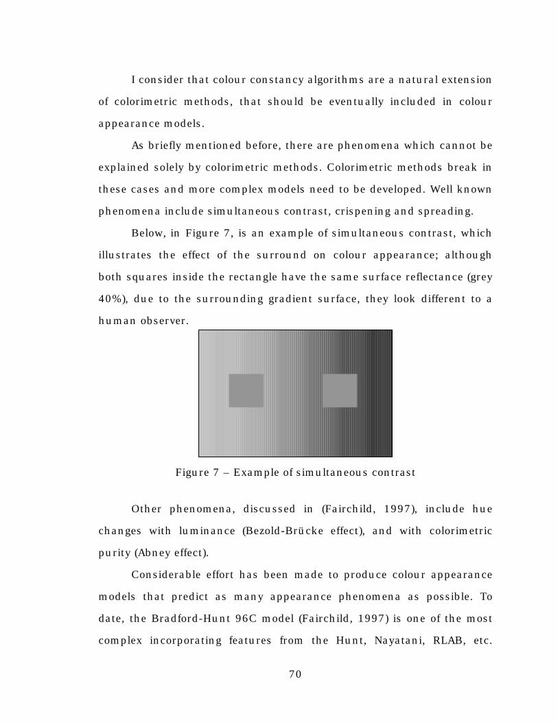
70

I consider that colour constancy algorithms are a natural extension

of colorimetric methods, that should be eventually included in colour

appearance models.

As briefly mentioned before, there are phenomena which cannot be

explained solely by colorimetric methods. Colorimetric methods break in

these cases and more complex models need to be developed. Well known

phenomena include simultaneous contrast, crispening and spreading.

Below, in Figure 7, is an example of simultaneous contrast, which

illustrates the effect of the surround on colour appearance; although

both squares inside the rectangle have the same surface reflectance (grey

40%), due to the surrounding gradient surface, they look different to a

human observer.

Figure 7 – Example of simultaneous contrast

Other phenomena, discussed in (Fairchild, 1997), include hue

changes with luminance (Bezold-Brücke effect), and with colorimetric

purity (Abney effect).

Considerable effort has been made to produce colour appearance

models that predict as many appearance phenomena as possible. To

date, the Bradford-Hunt 96C model (Fairchild, 1997) is one of the most

complex incorporating features from the Hunt, Nayatani, RLAB, etc.

71

models. However, I find it important to mention that all these complex

models assume that the tristimulus values of a reference white patch is

known. This implies that the colour constancy problem has been

previously solved.

All colour-constancy algorithms and all colour appearance models

are based on the presupposition that the phenomenon of colour

constancy is purely sensorial, i.e. the colour constancy mechanism

responds automatically to the visual stimuli. Of course, for machine

vision, this approach is natural, as it is difficult to extend a

computational model beyond its sensorial limits, into the realm of

cognition. However, in the case of the human visual system, it has been

established (Davidoff, 1991) that cognitive aspects play an important role

in colour appearance. For instance, memory colour, which refers to the

fact that human observers tend to remember specific colours for familiar

objects, such as skin, sky, etc., plays an important role in colour

appearance.

Other cognitive influence on appearance is caused by structural

effects. These effects, caused by the interpretation given to emerging

structures in the visual filed, can influence the perception of shapes as

well as colour. Below, in Figure 8, is an example of simultaneous

contrast in shape interpretation (Fairchild, 1997); both inner circles are

identical, but they appear of different sizes:

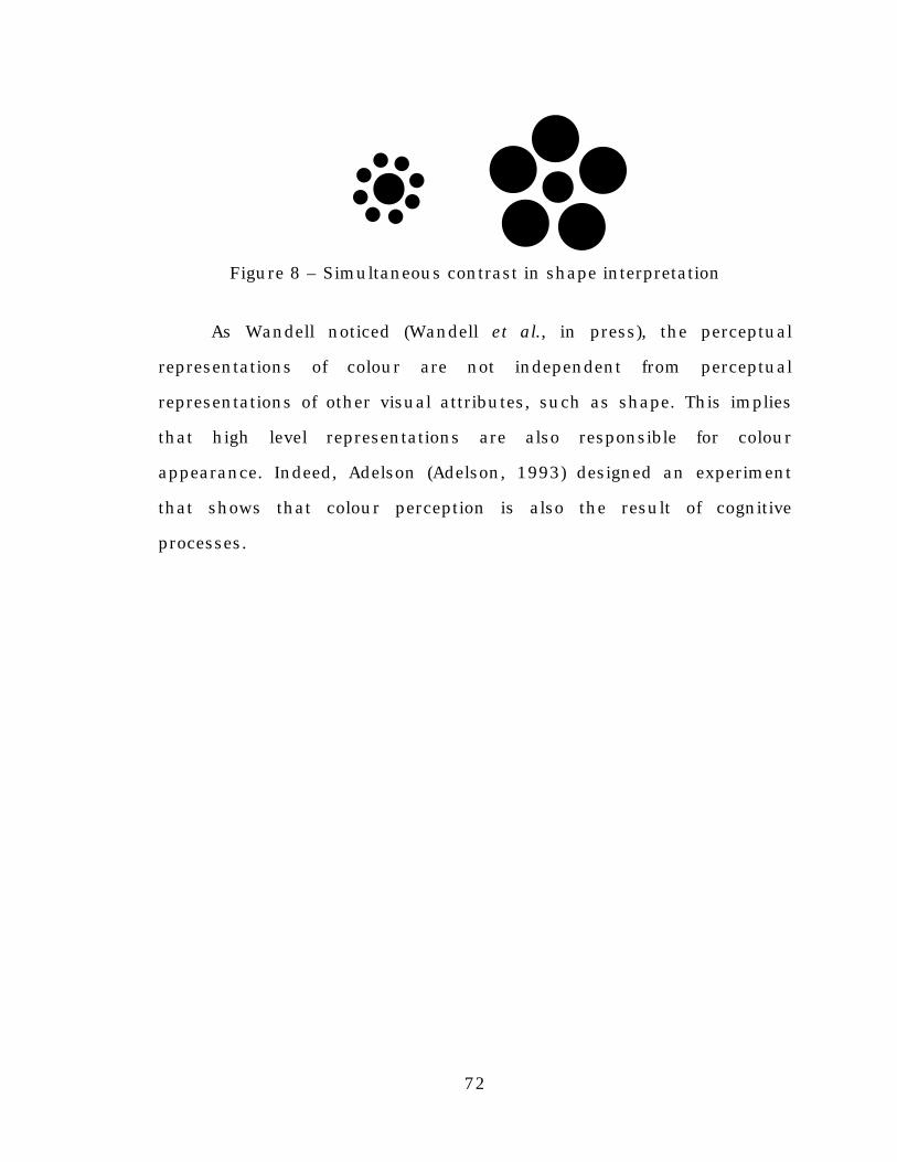
72

Figure 8 – Simultaneous contrast in shape interpretation

As Wandell noticed (Wandell et al., in press), the perceptual

representations of colour are not independent from perceptual

representations of other visual attributes, such as shape. This implies

that high level representations are also responsible for colour

appearance. Indeed, Adelson (Adelson, 1993) designed an experiment

that shows that colour perception is also the result of cognitive

processes.

73

Chapter 6

Theoretical Basis of Neural Networks: A Brief Review

In this chapter, neural networks are discussed in the context of

their applicability to colour vision and colour constancy. I will focus

mostly on multi-layer Perceptrons, since this is the neural network that

will be used in the rest of the thesis.

Although using a neural network instead of well-defined

mathematical models might seem less rigorous at a first glance, it

provides an alternative way for solving an under-constrained problem

such as colour constancy. Neural networks usually are a good choice for

problems where large quantities of data are available, but where a solid

theoretical model does not exist or is too complex.

6.1 Neurons and Neural Networks

Neural networks can be considered non-linear mapping systems.

Although originally inspired by biological neurons, most neural network

architectures and training algorithms are not biologically plausible, being

completely different than those of biological neural networks. This

implies that, even if an artificial neural network is able to perform the

same task as a biological neural network, such as colour constancy for

instance, there is no implication of any other similarity between the two

networks.

A neural network is usually composed of a set of inputs, an

internal processing structure and a set of outputs. The processing

structure, consisting of a set of neurons interconnected in a certain way

(the neural network architecture), acts like a “black box”, mapping the

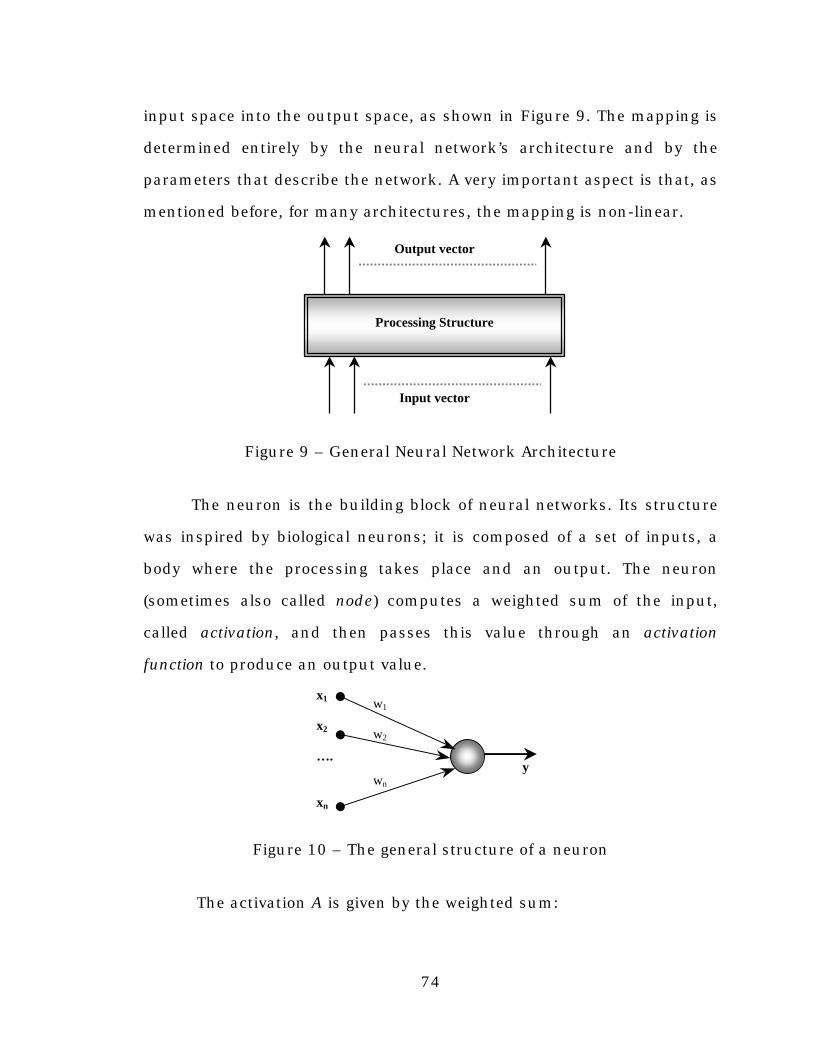
74

input space into the output space, as shown in Figure 9. The mapping is

determined entirely by the neural network’s architecture and by the

parameters that describe the network. A very important aspect is that, as

mentioned before, for many architectures, the mapping is non-linear.

Input vector

Output vector

Processing Structure

Figure 9 – General Neural Network Architecture

The neuron is the building block of neural networks. Its structure

was inspired by biological neurons; it is composed of a set of inputs, a

body where the processing takes place and an output. The neuron

(sometimes also called node) computes a weighted sum of the input,

called activation, and then passes this value through an activation

function to produce an output value.

x1

x2

… .

xn

y

w1

w2

wn

Figure 10 – The general structure of a neuron

The activation A is given by the weighted sum:

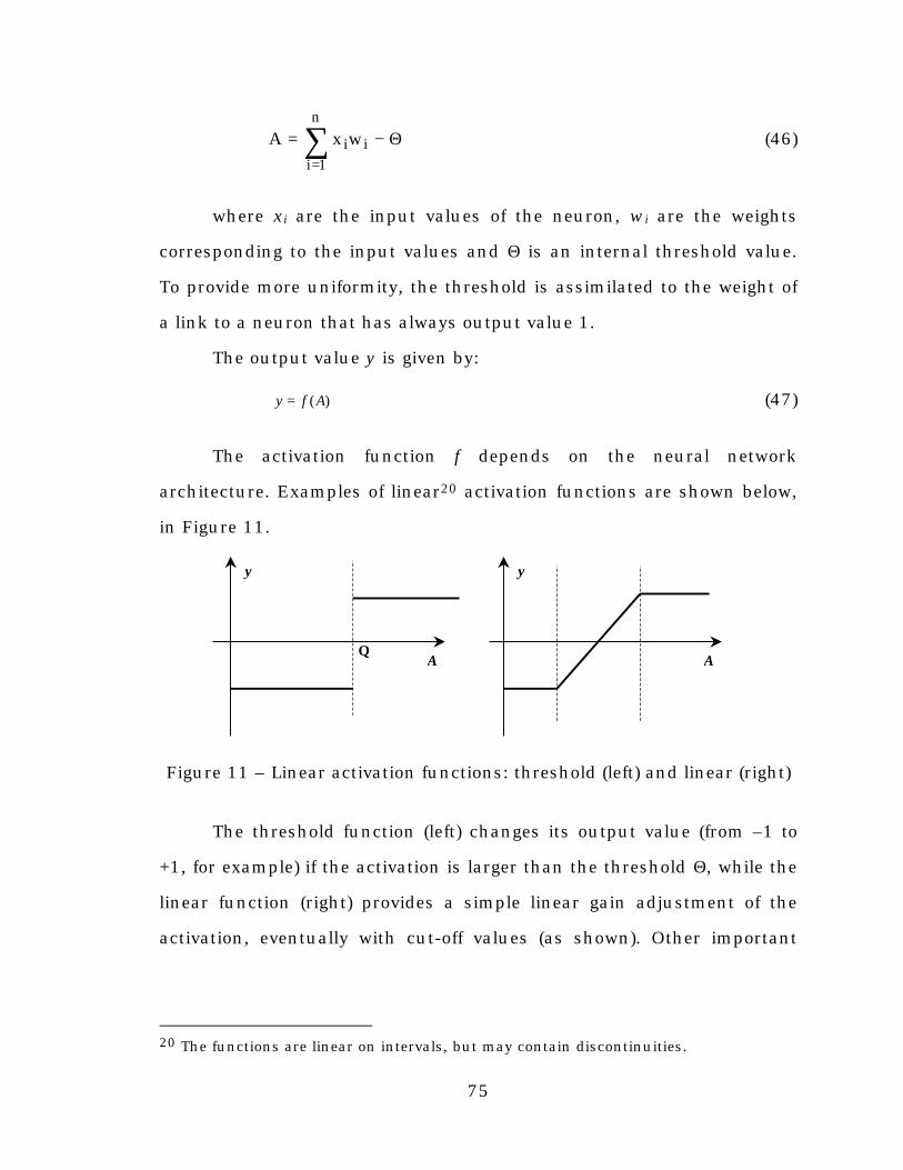
75

Θ−= ∑=

i

n

1iiwxA (46)

where xi are the input values of the neuron, wi are the weights

corresponding to the input values and Θ is an internal threshold value.

To provide more uniformity, the threshold is assimilated to the weight of

a link to a neuron that has always output value 1.

The output value y is given by:

)( Afy = (47)

The activation function f depends on the neural network

architecture. Examples of linear20 activation functions are shown below,

in Figure 11.

A A

y y

Θ

Figure 11 – Linear activation functions: threshold (left) and linear (right)

The threshold function (left) changes its output value (from –1 to

+1, for example) if the activation is larger than the threshold Θ , while the

linear function (right) provides a simple linear gain adjustment of the

activation, eventually with cut-off values (as shown). Other important

20 The functions are linear on intervals, but may contain discontinuities.

76

class of activation functions is that of sigmoid functions. This class

contains non-linear functions. The best known is:

Ae1

1y −+

= (48)

The function, shown in Figure 12, performs a non-linear compression ofreal values into the 0… 1 range:

0

0.2

0.4

0.6

0.8

1

-5 -4 -3 -2 -1 0 1 2 3 4 5

Figure 12 – The sigmoid function

This function is bounded between 0 and 1 and is easily

differentiable:

y’=A(1-A) (49)

These properties make the sigmoid function an ideal candidate for

the backpropagation training algorithm, that will be described below, in

section 6.3.

A single layer network is obtained by adding more neurons in

parallel. The inputs are connected to each neuron and the set of outputs

of the neurons represents the network’s output layer. Single layer

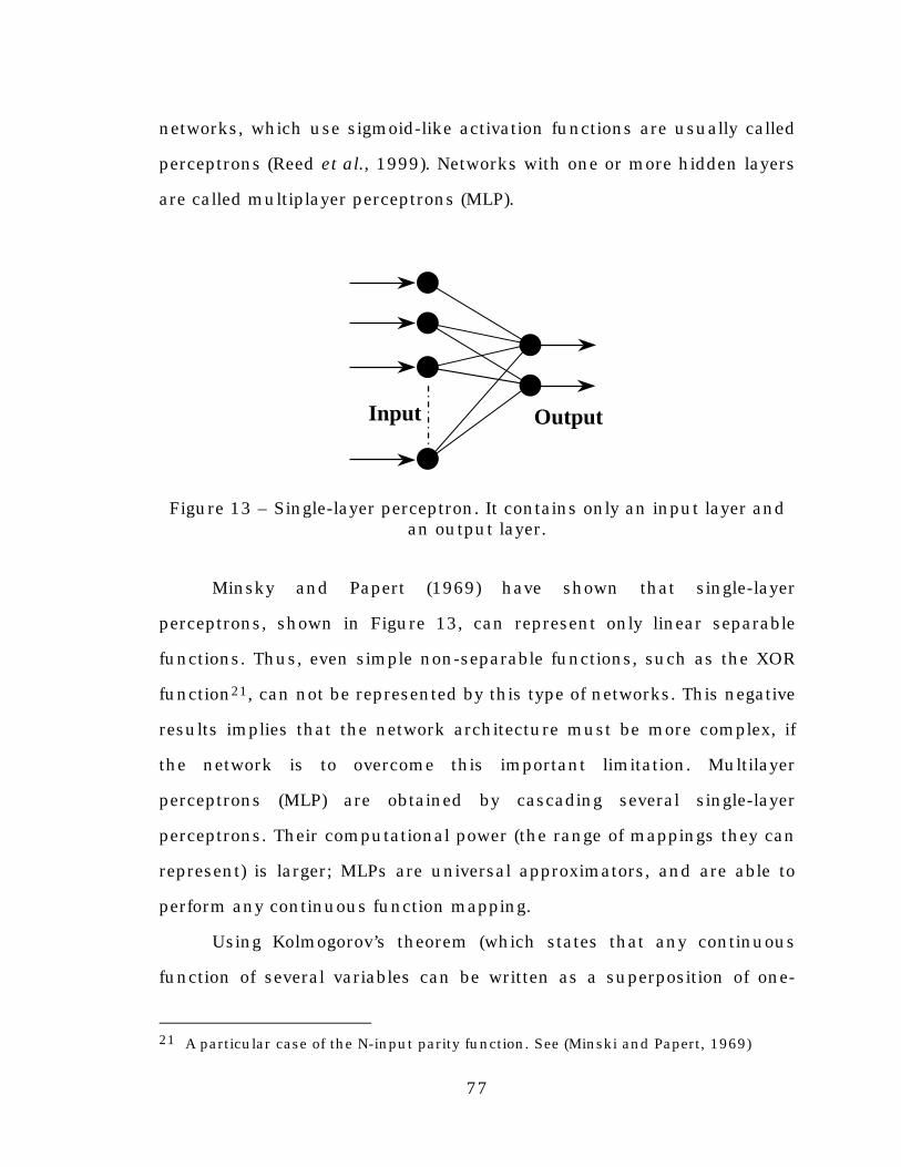
77

networks, which use sigmoid-like activation functions are usually called

perceptrons (Reed et al., 1999). Networks with one or more hidden layers

are called multiplayer perceptrons (MLP).

Input Output

Figure 13 – Single-layer perceptron. It contains only an input layer andan output layer.

Minsky and Papert (1969) have shown that single-layer

perceptrons, shown in Figure 13, can represent only linear separable

functions. Thus, even simple non-separable functions, such as the XOR

function21, can not be represented by this type of networks. This negative

results implies that the network architecture must be more complex, if

the network is to overcome this important limitation. Multilayer

perceptrons (MLP) are obtained by cascading several single-layer

perceptrons. Their computational power (the range of mappings they can

represent) is larger; MLPs are universal approximators, and are able to

perform any continuous function mapping.

Using Kolmogorov’s theorem (which states that any continuous

function of several variables can be written as a superposition of one-

21 A particular case of the N-input parity function. See (Minski and Papert, 1969)

78

variable functions of the original variables), Hecht-Nielsen has shown

that, in theory, one hidden layer is enough; any continuous mapping can

be implemented by a MLP with one hidden layer, which represents that

mapping. Although this is a very interesting theoretical result, in practice

it turns out that the required number of nodes in the hidden layer can be

very large. On the other hand, Lippmann has proven that two hidden

layers suffice: the first hidden layer divides the input space into half-

spaces, the second hidden layer intersects these half-spaces into convex

regions and the output layer unites them into arbitrary regions. Using

two hidden layers instead of one reduces the total number of neurons in

the network. The size of each layer and the number of nodes within

depends on the problem to be solved by the network. Although there are

some theoretical results that try to determine the best network

architecture, they do not guarantee the efficiency of the network or its

generalization power22.

6.2 The Backpropagation algorithm

The backpropagation algorithm (Rummelhart et al., 1986) is the

best known training algorithm used for MLPs. The algorithm, which is

equivalent to gradient descent, adjusts the weights and thresholds of the

neurons in a way that minimizes the difference23 between the actual

outputs of the neural network and the desired outputs, for a given set of

input patterns. The set of input patterns, together with the

22 For a detailed discussion, see (Reed et al., 1999).23 different metrics can be used to compute a distance in the output space.

79

corresponding desired (or ‘target’) outputs, is called the training set. The

description given below follows the proof from (Reed et al., 1999).

The neural network parameters (weights and thresholds) are

initialized with small random numbers. The training algorithm has two

steps. In the first step, the values presented at the inputs are propagated

to the output. In this feed-forward step, which is similar to the normal

operation of the network, no weights are changed. The output value of

node i (i.e. neuron i) is the weighted sum of its inputs (i.e. its activation)

mapped through a differentiable function (usually a sigmoid):

( )

== ∑

ijijii ywfAfy (50)

In the second step, the network’s output values are compared to

the desired values, for the corresponding input data, and an error is

computed. The most common error function used is ½ of the SSE:

( )∑ −=k

2kk yt

21

E (51)

where tk is the target for node k, and yk is the node’s actual output. The

derivative of E with respect to the node’s weights can be written as:

∑∑

∂∂⋅=

∂∂⋅

∂∂=

∂∂

k ij

kk

k ij

k

kij wA

wA

AE

wE δ (52)

where δk reflects the effect of Ak to the error, and can be computed for the

output nodes:

i

i

iii A

yyE

AE

∂∂

∂∂=

∂∂=δ (53)

80

For the output nodes, δk is obtained from equations 51 and 52:

( ) ( )kfyt kkk ′⋅−−=δ (54)

From equation 54, it can be noticed that f must be differentiable.

The sigmoid function has the derivative:

( )f1ff −⋅=′ (55)

For hidden nodes, δi can be obtained from:

∑∑

∂∂=

∂∂

∂∂=

∂∂=

k i

kk

k i

k

kii A

AAA

AE

AE δδ (56)

where k is over all output nodes. Given Ak, the activation of the output

node k (see equation 50), it follows that, if there is a link between node i

and node k, then:

kiii

k wfAA ⋅′=

∂∂

(57)

From equation 56, it follows that δi, for a node in the hidden layers,

is:

( )∑⋅′=k

kikii wf δδ (58)

Thus, equation 52 can be rewritten:

iik ij

kk

ijy

wA

wE δδ =

∂∂⋅=

∂∂ ∑ (59)

(the partial derivative in the sum is 0, if k≠i and is equal to yi if k=i).

81

After computing all partial derivatives (of E with respect to the

weights of the network), the weights are updated in the opposite direction

of the gradient:

ijij w

Ew

∂∂⋅−=∆ η (60)

η is called the learning rate, and is usually a sub-unitary positive

number. There is no method to compute the magnitude of η; a small η

will yield long training times and might trap the network in a local

minimum, while a large one will result in an unstable network, that

cannot converge. The proper magnitude is determined by the shape of

the error surface, the goal of backpropagation being to find the global

minimum on this surface.

The training set is presented to the neural network, one input-

output pair at a time, for several times (‘epochs’). The speed of the

learning process depends on many factors, and there are many optimized

versions of the ‘standard’ backpropagation algorithm. For a detailed

discussion, see (Reed et al., 1999).

Some of the algorithms are computationally very expensive,

because they take into account not only the first derivative of the error

but also the second derivative. The goal of these optimizations is not only

to improve the learning speed, but also to improve the network’s

stability; single-layer networks are guaranteed to converge to a solution,

but MLPs get sometimes trapped into local minima (in the error space)

and do not converge.

Due to the nature of the colour constancy problem, experiments

have shown that even the standard backpropagation algorithm is good

82

enough to train a neural network to solve this problem. The networks

trained with backpropagation always converged to a small average error,

below the target error. Accuracy problems encountered during testing

were not due to a poor training algorithm, but rather to the

underdetermined nature of colour constancy. Therefore, with two small

exceptions24 that will be mentioned in the following chapters, algorithms

that are more complex were not explored.

24 Experiments have shown that using different learning rates for each layer andhaving only partially connected layers improved the training speed.

83

Chapter 7

Learning Colour Constancy

7.1 Learning Colour Constancy with Neural Networks

From a computational perspective, the goal of colour constancy

can be defined as the transformation of a source image, taken under an

unknown illuminant, to a target image, identical to one that would have

been obtained by the same camera for the same scene under a standard

‘canonical’ illuminant.

The first stage of this process estimates the colour (or chromaticity)

of the illumination and the second stage corrects the image pixel-wise,

based on this estimate of the illuminant. Both stages can also be

combined into an equivalent process that estimates the matrix

transformation necessary to convert the image between the illuminants,

without explicitly estimating the illuminant.

From a physical perspective, colour constancy is an under-

determined problem. A camera looking at a surface with surface

reflectance S(λ) and illuminated by a light source with spectral power

distribution I(λ) will receive the following colour signal:

( ) ( ) ( )λλλ ISC ⋅= (61)

It is thus impossible to differentiate between the contribution of S

and I; for instance, a white surface under red light can yield the same

colour signal as a red surface under white light.

Moreover, the problem is complicated by the fact that the colour

signal C(λ) is integrated (similarly to the tristimulus integration

84

equations) with the camera sensor sensitivity functions (ρR, ρG and ρB for

a RGB colour camera) to produce the RGB pixel brightness value:

( ) ( ) ( ) ( ) ( )

( ) ( ) ( ) ( ) ( )

( ) ( ) ( ) ( ) ( )

⋅⋅⋅=⋅⋅=

⋅⋅⋅=⋅⋅=

⋅⋅⋅=⋅⋅=

∫∫∫ ∫∫ ∫

λλ

λ λ

λ λ

λλρλλλλρλ

λλρλλλλρλ

λλρλλλλρλ

dISdCB

dISdCG

dISdCR

BB

GG

RR

(62)

This integration sub-samples the colour signal to only three values:

R, G and B, introducing even more uncertainty. In this context, colour

correcting25 an image poses metamerism problems that must be taken

into account. Finlayson et al. (Finlayson et al., 1994a) have shown that

the transformation errors can be minimized by ‘sharpening’ the camera

sensors26. By using sharpened sensors, we can assume that the

transformation matrix that converts the image between the actual

illuminant and the canonical one is a diagonal matrix, similar to the von

Kries adaptation rule:

⋅

=

′′′

B

G

R

d00

0d0

00d

B

G

R

3

2

1

(63)

The only problem that remains to be solved is the accurate

estimation of the scene’s illuminant.

25 transforming the image from one illuminant to another one.26 see chapter 5.2 for details.

85

To estimate the illuminant, all colour constancy algorithms make

some a priori assumptions27, that add constraints to the space of

possible solutions. Some algorithms make explicit assumptions, such as

that there is a white surface in the scene, that the scene’s RGBs average

to grey, that that are specular reflectances in the scene, that the surface

reflectance functions and illuminant power spectra lie within low-

dimensional spaces, etc. These algorithms work well only when the

assumptions they rely upon are satisfied.

Other algorithms, like ‘gamut mapping’ or ‘colour by correlation’

make implicit assumptions, relying on prior surface and illuminant

distributions. Neural networks can provide an alternative to both types of

algorithms enumerated above. They are capable of learning non-linear

mappings that approximate any continuous function with any required

accuracy.

We use a neural network to learn the relationship between the

colours in a scene, given only by the RGB values in the digital image, and

the chromaticity of the illuminant under which the scene was taken

(Funt et al., 1996). After the illuminant is estimated, the whole image can

be colour corrected through a diagonal transformation.

The advantages of a neural network are that, on one hand, there

are no explicit assumptions regarding the scene content and, on the

other hand, the network can model eventual non-linear statistical

properties existent in the training set.

There are certain aspects, however, that are critical to the success

of a neural network system. First, data representation is very important,

27 see Chapter 5 for a detailed discussion on the algorithms.

86

because it determines the size of the network’s input and output layers.

Second, the neural network architecture must be chosen carefully; a too

large network requires a large training set and might not be able to

generalize due to overfitting (Hertz et al., 1991), while a too small

network will not be able to learn from the training set data.

7.2 Data Representation

A major requirement of the data representation of the input image

is that the representation be position invariant. That is, if the pixels in

the image are permutated, their representation should not change.

Another requirement is that the space be bounded, preferably between 0

and 1, to accommodate the neural network MLP architecture. And

finally, data representation should be compact; a sparse representational

space would only add to the input layer size of the MLP.

Since we are looking only for the illuminant chromaticity, the

absolute scene brightness is not required28. Thus, in our experiments,

we represented the data in the rg chromaticity space:

++= )BGR/(Gg

B)+G+R/(R=r(64)

This two dimensional space has the advantage that it is bounded

between 0 and 1, so it requires no additional pre-processing before being

28 Although the absolute brightness is not important, the relative brightness canprovide useful information, as in the 3D version of the gamut algorithm (Finlayson,1996)

87

input into the neural network. If necessary, the implicit blue

chromaticity component can be simply recovered from:

b r g= − −1 (65)

We also experimented with other chromaticity spaces, such as the

logarithmic perspective space (Finlayson, 1996), and obtained similar

illuminant estimation accuracy:

=

=

BG

logg

BR

logr(66)

Each RGB pixel from a digital image is projected into the rg

chromaticity space. This space is then uniformly sampled with a step

size S, so that all chromaticities within the same sampling square of size

S are taken as equivalent. Each sampling square maps to a distinct

network input node. The node is set either to 0 – indicating that an RGB

of chromaticity rg is not present in the scene, or 1– indicating that rg is

present. This quantification has the disadvantage that it forgoes some of

the resolution in chromaticity, but, on the other hand, it provides

permutation-independent inputs to the neural net, which is a major

advantage for both training and testing. A large sampling step S yields a

small quantified space, and consequently a small input layer for the

neural network, but it loses a lot of colour resolution, which in turn leads

to larger estimation errors. A small sampling step on the other hand,

yields a large input layer, which makes training very difficult.

Figure 14 and Figure 15 illustrate the representation in the rg

space of a scene taken under two different illuminants (a tungsten bulb

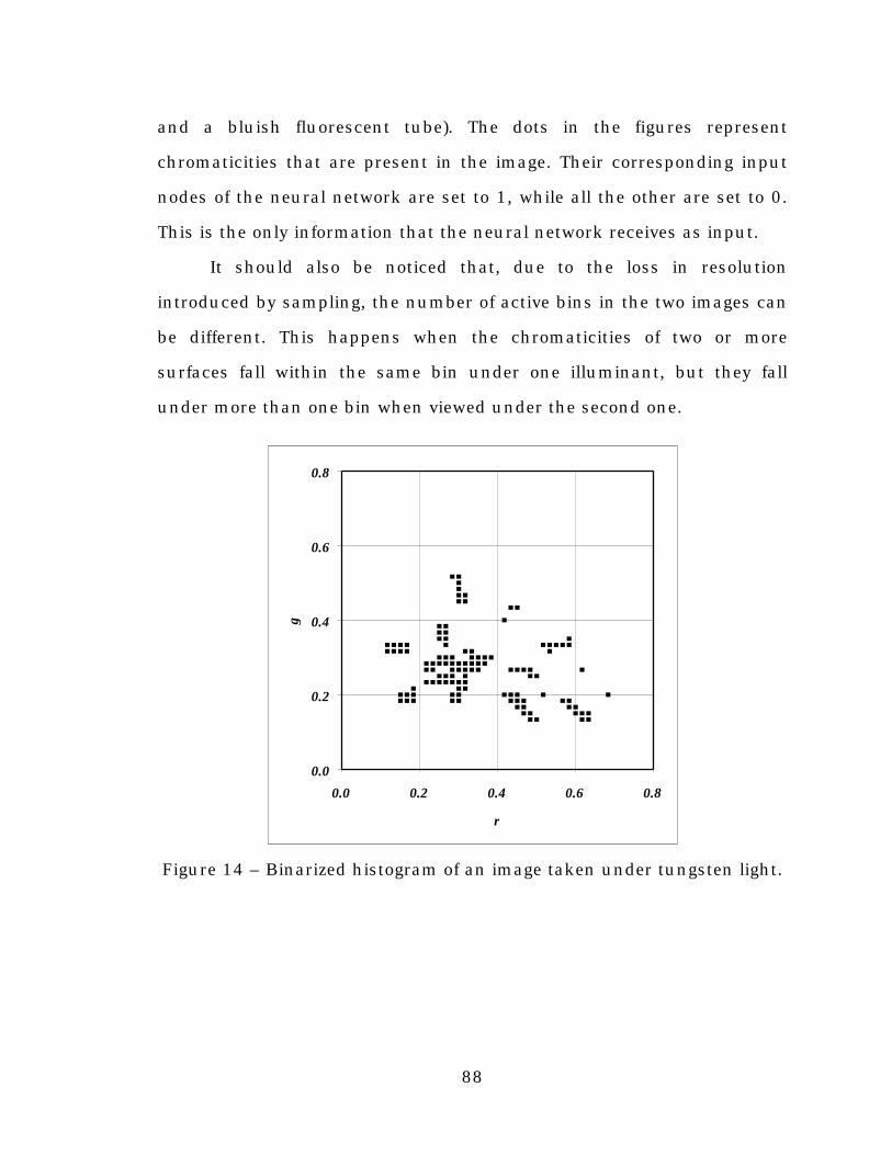
88

and a bluish fluorescent tube). The dots in the figures represent

chromaticities that are present in the image. Their corresponding input

nodes of the neural network are set to 1, while all the other are set to 0.

This is the only information that the neural network receives as input.

It should also be noticed that, due to the loss in resolution

introduced by sampling, the number of active bins in the two images can

be different. This happens when the chromaticities of two or more

surfaces fall within the same bin under one illuminant, but they fall

under more than one bin when viewed under the second one.

0.0

0.2

0.4

0.6

0.8

0.0 0.2 0.4 0.6 0.8

r

g

Figure 14 – Binarized histogram of an image taken under tungsten light.

89

0.0

0.2

0.4

0.6

0.8

0.0 0.2 0.4 0.6 0.8

r

g

Figure 15 – Binarized histogram of the same image taken under bluishfluorescent light.

7.3 The Neural Network Architecture

The neural network we used for all the experiments is a

multiplayer perceptron (MLP) with two hidden layers. All neurons have a

sigmoid activation function. Preliminary tests with other neural archi-

tectures, including a hybrid neural network that consisted of a self-

organizing map coupled with a MLP, did not yield satisfactory results.

The input layer consists of a large number of binary inputs

representing the presence or absence of a chromaticity in the scene. The

size NI of the input layer is related to S, but it is independent of the

image size:

2

S1

NI

= (67)

90

The first hidden layer contains 200–400 neurons and the second

layer around 20–40 neurons.

The output layer consists of only 2 neurons, corresponding to the

chromaticity values of the illuminant. This option was preferred over

having one neuron in the output layer for each illuminant in the

database, and using a binary encoding ( ‘1’ for the actual illuminant and

‘0’ for the others), because it is more compact and because it can

accommodate new illuminants without the need to retrain the whole

network.

The network architecture is described by sequences such as

‘3600-400-20-2’, meaning 3600 nodes in the input layer, 400 nodes in

the first hidden layer, 20 nodes in the second hidden layer and 2 nodes

in the output layer.

Input Layer

First Hidden Layer

Second Hidden Layer

Output Layer

Figure 16 – Neural Network Architecture: MLP with 2 hidden layers

The experiments, described in detail below, show that the size of

the layers (i.e. the number of neurons in each layer) can vary in a wide

range without affecting the performance of the networks.

91

7.4 Training the Neural Network

The neural network is trained using the backpropagation

algorithm, discussed in chapter 6. The error function used during

training and testing to measure the accuracy of the network is the

Euclidean distance in the rg-chromaticity space between the target and

the estimated illuminant. Since the rg space is not perceptually uniform,

errors in illuminant estimation might be perceived as having different

magnitudes, depending on the chromaticity of the actual illuminant.

Therefore, results will also be reported in the perceptually uniform CIE

Lab space. However, the network is trained to minimize errors in the rg

space and is not optimized for the Lab space.

In a first phase, the networks were trained and tested on synthetic

data. The data was generated from databases of surface reflectances and

of illuminant power spectra, corresponding to real data, measured with

a spectrometer with a 4nm sampling step in the 380nm–780nm range.

Both training and testing data sets consist of a large number of

scenes. Each scene consists of a random number of synthesized

surfaces. The RGB values of the surfaces within each scene are

generated by choosing a random illuminant Ek from the illuminant

database29 and integrating it with random selected surfaces Sj from the

surface reflectance database and with the camera sensors ρ:

Ri

ji

i

ki SER ρ⋅⋅= ∑ , G E Si

k

iij

iG= ⋅ ⋅∑ ρ and B E Si

k

iij

iB= ⋅ ⋅∑ ρ (68)

29 The same illuminant is used for all surfaces in the scene.

92

The surfaces correspond to matte reflectances and therefore have

only one rg chromaticity. Of course, the same surface has different

chromaticities under different illuminants, but it has only one

chromaticity when seen under a particular illuminant. This model is a

simplification of the real world case, where, due to noise, a flat matte30

patch will yield many more chromaticities scattered around the

theoretical chromaticity. The resulting RGB values (one RGB for each

surface in the scene) are then converted to the rg chromaticity space. In

the end, each scene is composed of a set of rg chromaticities and the

corresponding illuminant chromaticity.

During training, the training set is presented to the neural network

several times (‘epochs’). The surface chromaticities of each scene are

sampled with a sampling step S, binarized31, linearized32 and fed into the

network’s input layer. The corresponding illuminant chromaticity is the

target, whose r and g values should be obtained in the output layer.

7.5 Databases Used for Generating Synthetic Data

If testing is done on data generated from the same surface and

illuminant databases using the same sensor sensitivities, then any

databases and sensors can be used. However, our final goal was to test

the neural networks on real data, on natural scenes taken with a digital

camera. If a neural network, which is trained on synthetic data, is to be

tested on real images, the sensor sensitivity functions used to train it

30 If the surface is not flat, specular reflections must be taken into account (Lee, 1986)31 the elements have values of either 0 or 1 .32 The matrix corresponding the sampled and binarized rg space is converted to a one-dimensional array.

93

must be as close as possible to the real sensors. Any deviation of the real

camera from its model leads to deviations in the RGBs perceived by it

and, consequentially, to errors in the neural network illuminant

estimation. In this context, a SONY DCX-930 camera was carefully

calibrated and we used the obtained sensor sensitivity functions for

training and testing the networks. The graph below shows the relative

sensor sensitivity functions obtained for the SONY DCX-930 camera.

0

5000

10000

15000

20000

25000

380

420

460

500

540

580

620

660

700

740

780

nm

Rel

ativ

e S

ensi

tivity

REDGREENBLUE

Figure 17 – SONY DCX-930 senor sensitivity functions

The blue sensor is more sensitive than the other ones because the

camera is calibrated for an illuminant with temperature 3600K.

A camera is calibrated relative to an illuminant if it produces equal

R, G and B values for a reference white surface viewed under that

particular illuminant.

The illuminants in the database cover a wide range, from blue

fluorescent lights to reddish tungsten ones. Coloured filters were also

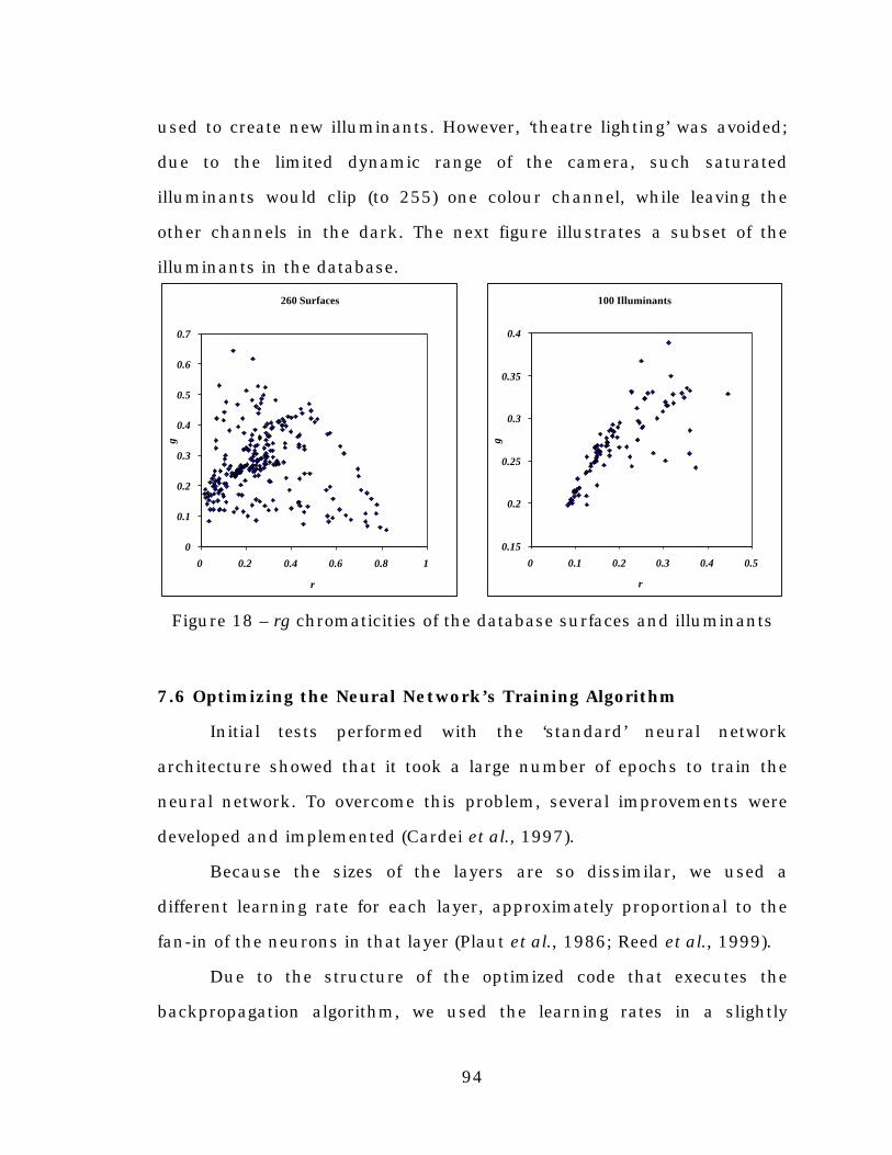
94

used to create new illuminants. However, ‘theatre lighting’ was avoided;

due to the limited dynamic range of the camera, such saturated

illuminants would clip (to 255) one colour channel, while leaving the

other channels in the dark. The next figure illustrates a subset of the

illuminants in the database.

260 Surfaces

0

0.1

0.2

0.3

0.4

0.5

0.6

0.7

0 0.2 0.4 0.6 0.8 1

r

g

100 Illuminants

0.15

0.2

0.25

0.3

0.35

0.4

0 0.1 0.2 0.3 0.4 0.5

r

g

Figure 18 – rg chromaticities of the database surfaces and illuminants

7.6 Optimizing the Neural Network’s Training Algorithm

Initial tests performed with the ‘standard’ neural network

architecture showed that it took a large number of epochs to train the

neural network. To overcome this problem, several improvements were

developed and implemented (Cardei et al., 1997).

Because the sizes of the layers are so dissimilar, we used a

different learning rate for each layer, approximately proportional to the

fan-in of the neurons in that layer (Plaut et al., 1986; Reed et al., 1999).

Due to the structure of the optimized code that executes the

backpropagation algorithm, we used the learning rates in a slightly

95

different manner, the rates being back-propagated from the output layer

to the input layer. Thus, with the exception of the learning rate

associated with the output layer (ηOut), the learning rates associated with

the first and second hidden layers (ηΗ 1 and ηH2) are given relative to ηOut.

The actual learning rate used in the backpropagation algorithm for

the second hidden layer is:

2HOut2H ηηη ⋅=′ (69)

The actual learning rate used in the backpropagation algorithm for the

first hidden layer is:

1H2HOut1H ηηηη ⋅⋅=′ (70)

The advantage of reporting relative learning rates is that it shows in an

explicit way the ratios between them.

We experimented with a wide range of learning rates, shown in

Table 1 (both actual and relative values are given), and concluded that

the network training is stable and that the values of the learning rates

have little impact on the accuracy of estimations. Of course, smaller

rates require a larger number of epochs for attaining the same accuracy.

The convergence of the backpropagation algorithm during training

with various neural network configurations was remarkable. Figure 19

and Figure 20 below show the variation of the average error during

training. The smoothly decreasing error curves illustrate the stability of

the networks.

96

0.005

0.01

0.015

0.02

0.025

0.03

0.035

1 2 3 4 5 6 7 8 9 10

Epochs

Err

or

20-1-0.25

20-1-0.50

20-1-1.00

20-5-0.25

20-5-0.50

20-5-1.00

Figure 19 – Convergence of the average error during training withdifferent learning rates (20-xx-xx).

0.005

0.01

0.015

0.02

0.025

0.03

0.035

1 2 3 4 5 6 7 8 9 10

Epochs

Err

or

5-1-0.25

5-1-0.50

5-1-1.00

5-5-0.25

5-5-0.50

5-5-1.00

Figure 20 – Convergence of the average error during training withdifferent learning rates (5-xx-xx).

97

Relative

Learning Rates

ηH2–ηH1–ηOut

Actual

Learning Rates

η'H2–η'H1–η'Out

20–1–0.25 5–0.25–0.25

20–1–0.50 10–0.50–0.50

20–1–1 20–1–1

20–5–0.25 25–1.25–0.25

20–5–0.50 50–2.50–0.50

20–5–1 100–5–1

10–1–0.25 2.50–0.25–0.25

10–1–0.50 5–0.50–0.50

10–1–1 10–1–1

10–5–0.25 12.50–1.25–0.25

10–5–0.50 25–2.50–0.50

10–5–1 50–5–1

5–1–0.25 1.25–0.25–0.25

5–1–0.50 2.50–0.50–0.50

5–1–1 5–1–1

5–5–0.25 6.25–1.25–0.25

5–5–0.50 12.50–2.50–0.50

5–5–1 25–5–1

Table 1 – Relative versus actual learning rates.

Figure 21 and Figure 22 are two charts that show the average

estimation errors of neural networks trained with all the learning rates

given in Table 1. Each graph, shown in, corresponds to a neural network

architecture:

• 2500–100–20–2

• 3600–200–40–2

98

The training data is composed of 20,000 scenes generated from a

database of 100 illuminants (200 scenes for each illuminant), 260

surface reflectances and the sensor sensitivity functions of a SONY DCX–

930 camera. Each scene is composed of 3 to 60 surfaces. The test set is

composed of 50,000 scenes (500 for each illuminant), each with 5 to 80

surfaces, synthesized from the same databases.

The performance of the neural network (NN) algorithms is also

compared with two other simple but intuitive algorithms: the ‘white

patch’ and the ‘grey world’ algorithms. The goal of the comparison is to

prove that, under controlled conditions, the network is able to learn to

estimate the chromaticity of the illuminant. Moreover, due to the

network’s superior performance, we presume that the learning is not

based merely on a neural simulation of either of these two algorithms. In

other tests, on real images, the network’s performance will also be

compared with more complex, high-performance, colour constancy

algorithms.

The white patch (WP) algorithm is based on a version of the retinex

algorithm (Land, 1977), which uses the maximum R, G and B values in

the scene to estimate the illuminant. The algorithm assumes that the

colour of the illuminant is given by the maximum values on each of the

three colour channels.

)max( iillum RR = ; )max( iillum GG = ; )max( iillum BB = (71)

where i is an index over all RGBs in the image.

If there is a perfect white surface in the scene, it will be the

brightest one and the algorithm will correctly estimate the illuminant as

having the colour of the white surfaces. If the scene contains no white

99

surfaces, then the accuracy of the algorithm depends on the scene’s

content, and the algorithm becomes inaccurate.

Our implementation of the ‘grey world’ (GW) algorithm estimates

the illuminant based on the average of all RGB values in the scene and

on an a priori known average, computed from the whole surface

reflectance database. The average RGB value in the scene, R , G and B ,

is compared with the database RGB average databaseRGB (the ‘world’

average), as seen under some known, canonical, illuminant RGBcanonical,

and any deviation of the scene average from this database average is

attributed to a change in the colour of the illuminant. Therefore, the

scene illuminant RGBillum is computed as:

⋅=

⋅=

⋅=

databasecanonicalillum

databasecanonicalillum

databasecanonicalillum

BB

BB

GG

GG

RR

RR

(72)

If the surfaces in the scene have the same average reflectance as

the ones in the database, than the algorithm makes an accurate estimate

of the illuminant. On the other hand, if the deviation of scene’s average

from the database average is caused by the distribution of surface

colours in the scene, than the estimate is not accurate. In general, in the

case of erroneous estimates, the grey world algorithm has the tendency

to wash out the colours in that scene. For instance, an image of a blue

sky or a blue sea will be interpreted as an image taken under a blue

illuminant and the image will be colour corrected such that, in the end,

the average colour in the scene is equal to the database average, which is

100

usually grey. The database average depends only on the colour of the

surfaces in the database and is independent of the canonical illuminant.

It may be argued that the comparison between the neural networks

and the grey world (GW) and white patch (WP) algorithms is not fair,

because the neural network is much more complex than these

algorithms.

However, both GW and WP algorithms benefit by the test scenario.

Statistically, the estimation errors of both WP and GW algorithms

converge to zero as the number of surfaces in the scene approaches the

size of the database. This happens because, in the case of the WP

algorithm, there is a high chance of having a white surface in the scene

(there is a reference white surface in the database), while in the case of

the GW algorithm, the scene average converges to the database average

as the number of surfaces in the scene approaches the size of the

database.

101

0.0000 0.0050 0.0100 0.0150 0.0200 0.0250 0.0300 0.0350

GW

WP

NN: 20-1-0.25

NN: 20-1-0.50

NN: 20-1-1.00

NN: 20-5-0.25

NN: 20-5-0.50

NN: 20-5-1.00

NN: 10-1-0.25

NN: 10-1-0.50

NN: 10-1-1.00

NN: 10-5-0.25

NN: 10-5-0.50

NN: 10-5-1.00

NN: 5-1-0.25

NN: 5-1-0.50

NN: 5-1-1.00

NN: 5-5-0.25

NN: 5-5-0.50

NN: 5-5-1.00

Average Error

Figure 21 – Average estimation errors for neural networks trained withvarious learning rates. The network architecture is: 2500–100–20–2. The

networks are compared against the WP and GW algorithms.

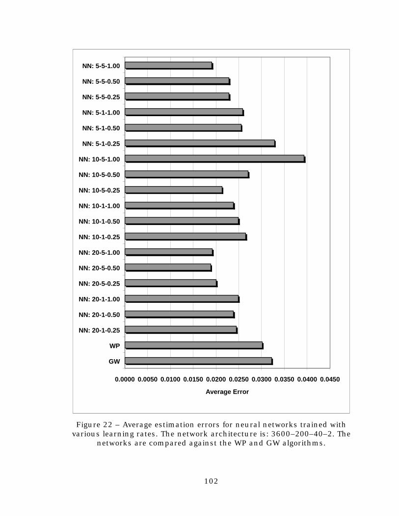
102

0.0000 0.0050 0.0100 0.0150 0.0200 0.0250 0.0300 0.0350 0.0400 0.0450

GW

WP

NN: 20-1-0.25

NN: 20-1-0.50

NN: 20-1-1.00

NN: 20-5-0.25

NN: 20-5-0.50

NN: 20-5-1.00

NN: 10-1-0.25

NN: 10-1-0.50

NN: 10-1-1.00

NN: 10-5-0.25

NN: 10-5-0.50

NN: 10-5-1.00

NN: 5-1-0.25

NN: 5-1-0.50

NN: 5-1-1.00

NN: 5-5-0.25

NN: 5-5-0.50

NN: 5-5-1.00

Average Error

Figure 22 – Average estimation errors for neural networks trained withvarious learning rates. The network architecture is: 3600–200–40–2. The

networks are compared against the WP and GW algorithms.

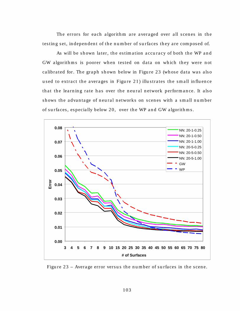
103

The errors for each algorithm are averaged over all scenes in the

testing set, independent of the number of surfaces they are composed of.

As will be shown later, the estimation accuracy of both the WP and

GW algorithms is poorer when tested on data on which they were not

calibrated for. The graph shown below in Figure 23 (whose data was also

used to extract the averages in Figure 21) illustrates the small influence

that the learning rate has over the neural network performance. It also

shows the advantage of neural networks on scenes with a small number

of surfaces, especially below 20, over the WP and GW algorithms.

0.00

0.01

0.02

0.03

0.04

0.05

0.06

0.07

0.08

3 4 5 6 7 8 9 10 15 20 25 30 35 40 45 50 55 60 65 70 75 80

# of Surfaces

Err

or

NN: 20-1-0.25

NN: 20-1-0.50

NN: 20-1-1.00

NN: 20-5-0.25

NN: 20-5-0.50

NN: 20-5-1.00

GW

WP

Figure 23 – Average error versus the number of surfaces in the scene.

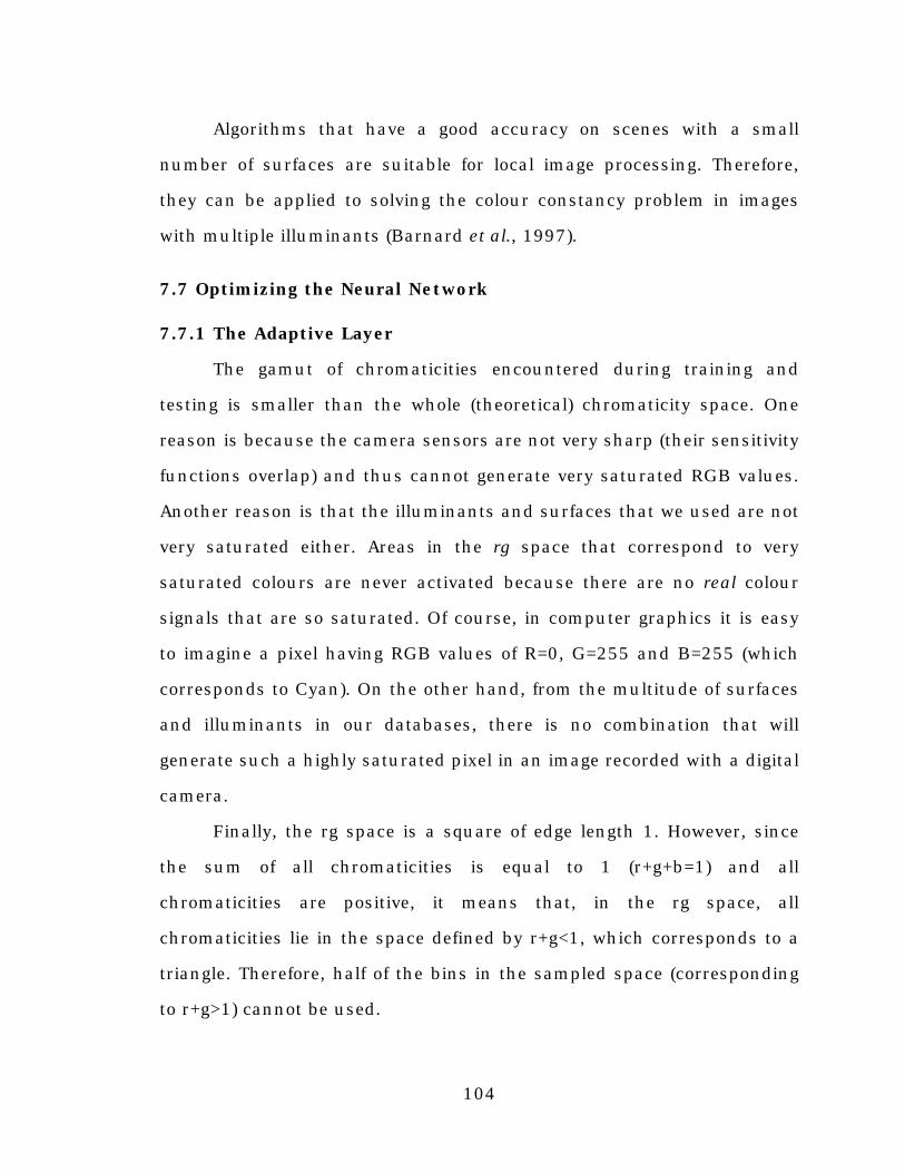
104

Algorithms that have a good accuracy on scenes with a small

number of surfaces are suitable for local image processing. Therefore,

they can be applied to solving the colour constancy problem in images

with multiple illuminants (Barnard et al., 1997).

7.7 Optimizing the Neural Network

7.7.1 The Adaptive Layer

The gamut of chromaticities encountered during training and

testing is smaller than the whole (theoretical) chromaticity space. One

reason is because the camera sensors are not very sharp (their sensitivity

functions overlap) and thus cannot generate very saturated RGB values.

Another reason is that the illuminants and surfaces that we used are not

very saturated either. Areas in the rg space that correspond to very

saturated colours are never activated because there are no real colour

signals that are so saturated. Of course, in computer graphics it is easy

to imagine a pixel having RGB values of R=0, G=255 and B=255 (which

corresponds to Cyan). On the other hand, from the multitude of surfaces

and illuminants in our databases, there is no combination that will

generate such a highly saturated pixel in an image recorded with a digital

camera.

Finally, the rg space is a square of edge length 1. However, since

the sum of all chromaticities is equal to 1 (r+g+b=1) and all

chromaticities are positive, it means that, in the rg space, all

chromaticities lie in the space defined by r+g<1, which corresponds to a

triangle. Therefore, half of the bins in the sampled space (corresponding

to r+g>1) cannot be used.

105

We modified the neural network’s architecture, such that it

receives input only from the active nodes (i.e. the input nodes that were

activated at least once during training). The inactive nodes (i.e. those

nodes that were not activated at any time during training) are pruned

from the neural network, together with their links to the first hidden

layer.

In the current implementation, the network’s architecture is

actually modified in a pre-processing stage before the first training

epoch, during a pass through all the data in the training set. After this

stage, the links from the first hidden layer are directed only towards the

neurons in the input layer that are active, i.e. those that correspond to

existing chromaticities, while links to inactive nodes are eliminated.

Input Layer

First Hidden Layer

Second Hidden Layer

Output Layer

Inactive Nodes

Pruned Links

Figure 24 – The adaptive layer. The first hidden layer adapts its links tothe active nodes in the input layer, pruning unused links.

106

The number of active nodes depends on the databases used to

generated the data and on the shape of the sensor sensitivity functions.

The pre-processing done before the actual training is equivalent to

eliminating the links to inactive nodes during training, since the

contribution of the inactive nodes to the neural activations in the first

hidden layer is always equal to zero.

Table 2 shows the number of active and inactive nodes as a

function of NI, the total number of nodes, for typical data generated

using the sensor sensitivity functions of a SONY DXC-930 digital camera.

NI ActiveNodes

InactiveNodes

400 166 234

625 258 367

900 351 549

1600 601 999

2500 909 1591

3600 1255 2345

4900 1673 3227

Table 2 – Active and inactive nodes, versus the total numberof nodes in the input layer (NI)

Having less nodes and less links in the network shortens the

training time significantly (about 4-6 times, in our experiments). It might

be argued that some chromaticities that never showed up during training

might appear in some scenes during testing. In this case, the above

mentioned approach would simply ignore them, since there are no links

from their input nodes (inactive during training) and the rest of the

network. On the other hand, a fully connected network will introduce

107

some noise to the rest of the network through the links of those nodes

(since their weights have never been trained, the signal that is being

propagated through the network from these nodes can be interpreted as

noise).

7.7.2 Optimizing the Neural Network’s Architecture

The size of the input layer is determined by the compromise

between the chromaticity resolution and the training time (which is a

function of the network’s size). For a sampling step S, the rg space is

divided into S2 squares of edge S; S becomes the best attainable

chromaticity resolution, for the input data. We experimented with input

layer sizes, ranging from 400 to 4900. This corresponds to S ranging

from 0.014 to 0.05 (1/70 to 1/20).

The goal of the experiments was to determine the influence of the

input layer size on the accuracy of the illuminant estimations. All

networks have ‘xxxx-200-20-2’ architectures, where ‘xxxx’ is the size of

the input layer. The networks are almost fully connected; all nodes within

a layer are linked to all nodes from the previous layer, with the exception

of the first hidden layer, which is connected only to the active nodes from

the input layer. The actual number of active nodes for each configuration

is given in Table 2.

All networks were trained for 20 epochs to assure good learning

and network stability. The training data is composed of 50,000 scenes

generated from a database of 100 illuminants (500 scenes for each

illuminant), 260 surface reflectances and the sensor sensitivity functions

taken form the SONY DCX-930 camera. Each scene is composed of 3 to

108

60 surfaces. The test set is composed of 50,000 scenes (500 for each

illuminant), each with 5 to 80 surfaces, synthesized from the same

databases. The graph below shows the average estimation errors for the

networks we tested. The results are also compared against the WP and

GW algorithms.

0.0000 0.0050 0.0100 0.0150 0.0200 0.0250 0.0300 0.0350

NI=400

NI=625

NI=900

NI=1600

NI=2500

NI=3600

NI=4900

GW

WP

(Weighted) Average Error

Figure 25 – The influence of the input layer (NI) on the neural networkperformance

Again, the size of the input layer has a small influence on the

estimation accuracy. From the several architectures we experimented on,

we continued our experiments with networks with NI equal to 1600,

2500 and, sometimes, 3600. The network with NI=4900 took a very long

time to train (due to its large size) and smaller networks yielded larger

estimation errors.

109

The next experiment was designed to find the optimum size for the

first hidden layer. We tested two different network architectures:

‘1600–xxx–20–2’ and ‘2500–xxx–20–2’, where ‘xxx’ is the size of the first

hidden layer (H1).

We experimented with H1 equal to 50, 100, 150, 200, and 250. The

number of links to the input layer was again dictated by the number of

active nodes. We used the same training and testing data sets as before.

The accuracy is almost identical for all network architectures, and

much better than the accuracy of the GW and WP algorithms.

The results are shown in the following two graphs:

0.000 0.005 0.010 0.015 0.020 0.025 0.030 0.035

H1=25

H1=50

H1=100

H1=150

H1=200

H1=250

GW

WP

Figure 26 – The influence of the first hidden layer (H1) on the neuralnetwork performance. The input layer is of size NI=1600.

110

0.000 0.005 0.010 0.015 0.020 0.025 0.030 0.035

H1=25

H1=50

H1=100

H1=150

H1=200

H1=250

GW

WP

Figure 27 – The influence of the first hidden layer (H1) on the neuralnetwork performance. The input layer is of size NI=2500.

The next experiment, similar to the ones described above, was

designed to find the optimum size for the second hidden layer. We tested

four different network architectures: ‘1600–50–xx–2’, ‘1600–100–xx–2’,

‘2500–50–xx–2’ and ‘2500–100–xx–2’, where ‘xx’ is the size of the second

hidden layer (H2).

We experimented with H2 of size 5, 10, 20, 30, 40 and 50. The

second layer is fully connected to the first hidden layer. The number of

links from the first hidden layer to the input layer was again dictated by

the number of active nodes. We used the same training and testing data

sets as before. The results are shown in the following four graphs:

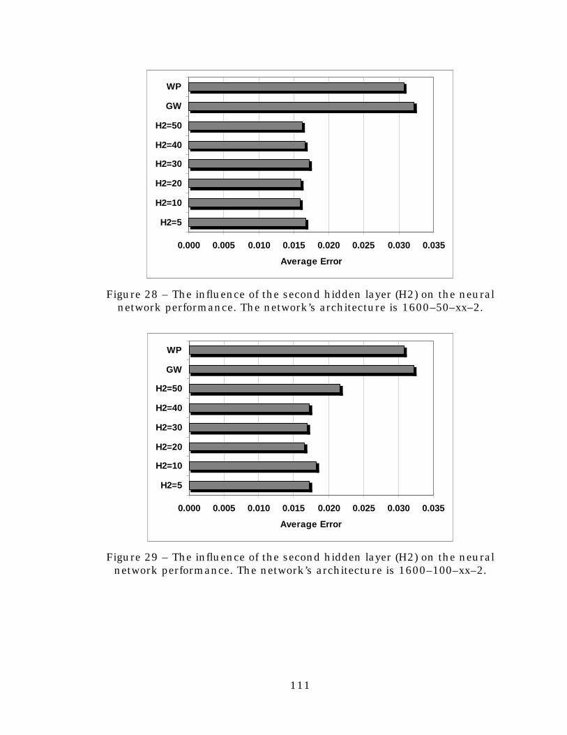
111

0.000 0.005 0.010 0.015 0.020 0.025 0.030 0.035

H2=5

H2=10

H2=20

H2=30

H2=40

H2=50

GW

WP

Average Error

Figure 28 – The influence of the second hidden layer (H2) on the neuralnetwork performance. The network’s architecture is 1600–50–xx–2.

0.000 0.005 0.010 0.015 0.020 0.025 0.030 0.035

H2=5

H2=10

H2=20

H2=30

H2=40

H2=50

GW

WP

Average Error

Figure 29 – The influence of the second hidden layer (H2) on the neuralnetwork performance. The network’s architecture is 1600–100–xx–2.

112

0.000 0.005 0.010 0.015 0.020 0.025 0.030 0.035

H2=5

H2=10

H2=20

H2=30

H2=40

H2=50

GW

WP

Average Error

Figure 30 – The influence of the second hidden layer (H2) on the neuralnetwork performance. The network’s architecture is 2500–50–xx–2.

0.000 0.005 0.010 0.015 0.020 0.025 0.030 0.035

H2=5

H2=10

H2=20

H2=30

H2=40

H2=50

GW

WP

Average Error

Figure 31 – The influence of the second hidden layer (H2) on the neuralnetwork performance. The network’s architecture is 2500–100–xx–2.

Again, the difference between the performance of the networks we

tested is very small, and all networks have a much better accuracy than

the WP and GW algorithms.

113

All the results presented above are statistically significant for the

data the network was trained and tested on (i.e. surfaces, illuminants

and the shape of camera sensors). For different data, such as data

corresponding to other cameras or different surface and illuminant

databases, the results can vary.

The experiments show that, except for some minor variations in

accuracy, all networks are almost insensitive to variations in architecture

and in learning rates, at least in the range we experimented on. This

leads us to the conclusion that for future experiments, the architecture

of the neural networks is not critical. The next chapters will show that

accuracy of illuminant estimates on real images, using neural networks,

depends on an accurate modelling of the colours present in those real

images.

7.8 Testing the Neural Network on Real Images

The previous section has shown that neural networks have a much

better performance than the other algorithms they were compared

against. Not only are they more accurate, but their architectural

parameters, such as the number of nodes in the input or hidden layers,

can vary within a wide range, without large changes in the performance.

In the next phase, we tested the neural networks on real images.

Unlike synthesized images, where the environment is completely

controlled, real images pose a number of problems for colour constancy

algorithms. Noise, specularities, errors in camera calibration, colour

distributions, lens flare, fluorescent surfaces, can all lead to deviations of

the image RGBs from their ideal values.

114

We tested the neural network on 48 images taken with a SONY

DXC-930 CCD camera under controlled conditions. The chromaticity of

the illuminant was assumed to be the same as the chromaticity of a

reference white patch seen under the same illuminant. The images were

taken under a wide range of light sources, from fluorescent lights with

blue filters to tungsten ones.

The images were pre-processed before being passed to the network,

to attenuate much of the noise inherent in real images. Digital cameras

have a smaller dynamic range than human eye or even than film.

Therefore, the bright areas in images can be too bright to fit on a 0 to

255 scale without sacrificing the average brightness of the image. This

produces colour shifts for these bright pixels; the general tendency is to

desaturate the colour and shift all chromaticities toward white. Similarly,

dark regions in the image have a small signal to noise ratio and can

produce large and unpredictable chromaticity shifts.

Therefore, the clipped (i.e. pixels having values of 255 on any R, G

or B colour channels) and the very dark pixels are ignored by the colour

constancy algorithms that we tested. A threshold pixel value of 7 (on a 0

to 255 scale) on any of the three RGB colour channels was used to

eliminate dark pixels. The images were also smoothed by local averaging,

to eliminate noisy pixels. The window size was of 5 pixels. After pre-

processing, each image contained around 10,000 valid pixels that were

passed to the network (and to the other algorithms). Due to the sampling

size of the chromaticity histogram, the number of active nodes in the

neural network, for any image in the test set, reaches around 60 to 120

(i.e. distinct binarized histogram bins). This number is less than the total

number of nodes that were active during the training on synthetic data.

115

This can be explained by the fact that not all surfaces and illuminants

encountered during training were in the real images and, most

importantly, that during training on synthetic data, noise and clipped

pixels were not an issue and all RGB values in the scenes were taken

into account. On the other hand, for real images, we ignored very

saturated pixels, since there is no possibility to differentiate between

such saturated pixels and noise.

Table 3 shows the results on real images. The mean distance error

represents the average Euclidean distance between the estimated and

actual illuminants in rg chromaticity space. The standard deviation is

also reported.

To relate these results to the human perception of the colour

difference between the estimated and the actual illuminants, the mean

∆ELab errors in the perceptually uniform CIE Lab space are also

presented. The ∆ELab error is taken between the colour of the estimated

illuminant and the colour of the actual one, under the following

assumptions. First, we assume that both illuminants are displayed on a

sRGB compliant monitor33 (Anderson et al., 1996) and, second, that both

illuminants have the same luminance, in CIE XYZ coordinates (for this

experiment, we chose Y=100). The conversion from the RGB space to the

Lab colour space was done by converting the RGB values to sRGB and

then to CIE XYZ and to CIE Lab. The conversion from XYZ to Lab was

done based on equations 6–8.

33 e.g. a sRGB calibrated monitor

116

The illumination chromaticity variation (#1) shows the average

shift in the rg chromaticity space between a pre-determined canonical

illuminant and the correct illuminants. This can be considered as a

‘worst case’ estimation, where we pick an a priori illuminant and consider

that it is the illuminant that was used in all images. In our experiments,

the canonical illuminant was selected to be the one for which the CCD

camera was calibrated (i.e. a white patch had identical intensity values

on all three colour channels). A different choice could have been the

average illuminant in the test images, which would have minimized the

estimation errors. However, we chose the illuminant for which the

camera is calibrated instead of the average illuminant for two reasons.

First, the average illuminant varies with the images in the test set;

whereas, the canonical is fixed for a given camera. Second, by using the

illuminant for which the camera is calibrated, we can see the errors that

would be obtained if the images were not colour corrected.

The grey world algorithm (#2) has to rely only on a model based on

prior knowledge gathered from the surface database. The results show

that the particular colour distributions found in the surface and

illuminant databases do not match the real world distributions of

surfaces and illuminants. The white-patch algorithm (#3) suffered

because of clipped pixels, noise and the fact that the “whitest” patch may

not be truly white.

The results for the neural network (#4) were obtained using the

neural network architecture ‘3600–200–50–2’. The network was trained

on the same training sets used for the networks that were tested on

synthesized data, as described in the previous sections.

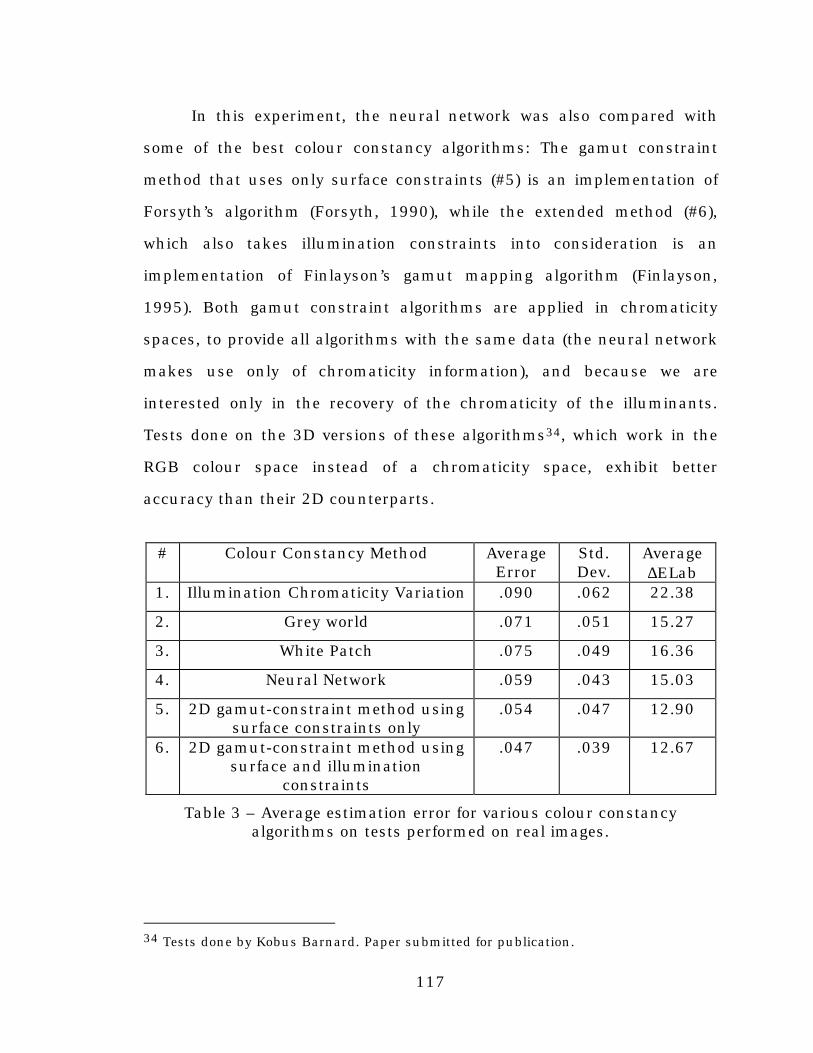
117

In this experiment, the neural network was also compared with

some of the best colour constancy algorithms: The gamut constraint

method that uses only surface constraints (#5) is an implementation of

Forsyth’s algorithm (Forsyth, 1990), while the extended method (#6),

which also takes illumination constraints into consideration is an

implementation of Finlayson’s gamut mapping algorithm (Finlayson,

1995). Both gamut constraint algorithms are applied in chromaticity

spaces, to provide all algorithms with the same data (the neural network

makes use only of chromaticity information), and because we are

interested only in the recovery of the chromaticity of the illuminants.

Tests done on the 3D versions of these algorithms34, which work in the

RGB colour space instead of a chromaticity space, exhibit better

accuracy than their 2D counterparts.

# Colour Constancy Method AverageError

Std.Dev.

Average∆ELab

1. Illumination Chromaticity Variation .090 .062 22.38

2. Grey world .071 .051 15.27

3. White Patch .075 .049 16.36

4. Neural Network .059 .043 15.03

5. 2D gamut-constraint method usingsurface constraints only

.054 .047 12.90

6. 2D gamut-constraint method usingsurface and illumination

constraints

.047 .039 12.67

Table 3 – Average estimation error for various colour constancyalgorithms on tests performed on real images.

34 Tests done by Kobus Barnard. Paper submitted for publication.

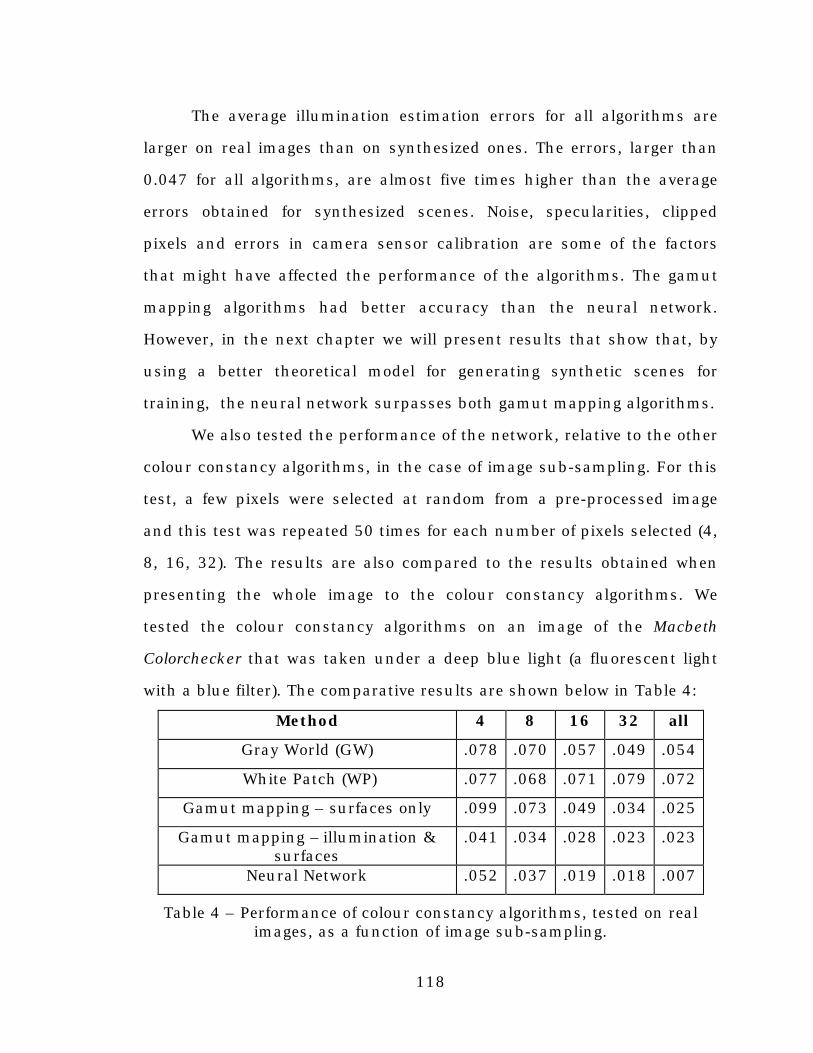
118

The average illumination estimation errors for all algorithms are

larger on real images than on synthesized ones. The errors, larger than

0.047 for all algorithms, are almost five times higher than the average

errors obtained for synthesized scenes. Noise, specularities, clipped

pixels and errors in camera sensor calibration are some of the factors

that might have affected the performance of the algorithms. The gamut

mapping algorithms had better accuracy than the neural network.

However, in the next chapter we will present results that show that, by

using a better theoretical model for generating synthetic scenes for

training, the neural network surpasses both gamut mapping algorithms.

We also tested the performance of the network, relative to the other

colour constancy algorithms, in the case of image sub-sampling. For this

test, a few pixels were selected at random from a pre-processed image

and this test was repeated 50 times for each number of pixels selected (4,

8, 16, 32). The results are also compared to the results obtained when

presenting the whole image to the colour constancy algorithms. We

tested the colour constancy algorithms on an image of the Macbeth

Colorchecker that was taken under a deep blue light (a fluorescent light

with a blue filter). The comparative results are shown below in Table 4:

Method 4 8 16 32 all

Gray World (GW) .078 .070 .057 .049 .054

White Patch (WP) .077 .068 .071 .079 .072

Gamut mapping – surfaces only .099 .073 .049 .034 .025

Gamut mapping – illumination &surfaces

.041 .034 .028 .023 .023

Neural Network .052 .037 .019 .018 .007

Table 4 – Performance of colour constancy algorithms, tested on realimages, as a function of image sub-sampling.

119

The results presented above show the accuracy of the neural

network when tested on images with a small number of surfaces. This

implies that neural networks can also be used in images with multiple

illuminants (Barnard et al., 1997).

7.9 Independent Tests on Synthetic and Real Data

In a series of experiments, Kobus Barnard (Barnard, 1999)

compared a wide range of 2D and 3D colour constancy algorithms,

including neural networks. From those experiments, we present results

obtained by the gamut constraint method35 that uses only surface

constraints (Forsyth, 1990), various versions of the extended gamut

constraint method, which also takes illumination constraints into

consideration (Finlayson, 1995), four neural networks and two

correlation methods (Finlayson, 1997).

Two neural networks were trained on synthetic data for each of the

following two architectures:

• ‘1600–50–20–2’, with 608 links from each node in the first hidden

layer to the input layer (corresponding to the maximum number of

active nodes in the input layer). This architecture was used for

networks [1] and [3] in the table below.

• ‘2500–50–20–2’, with 948 links from each node in the first hidden

layer to the input layer (corresponding to the maximum number of

active nodes in the input layer). This architecture was used for

networks [2] and [4] in the table below.

35 also called ‘gamut mapping’, although this term is also used to describe the colourmapping between imaging devices.

120

Each network was trained for ten epochs on one of four different

data sets of 100,000 scenes. Two networks ([1] and [2] in table below)

were trained on data containing no noise and no specularities36, and two

networks ([3] and [4] in table below) were trained on data containing

random amounts of maximum 5% white noise and maximum 25%

specular reflections. One of the correlation methods used a binary (0/1)

correlation matrix, while the second one used Gaussian distributions in

the correlation matrix.

The ‘Illumination Chromaticity Variation’ shows the average shift

in the rg chromaticity space between a pre-determined canonical

illuminant and the correct illuminants. It is the error obtained if no

colour correction is performed. The ‘Average Illumination’ shows the

error obtained if the average database illuminant is considered to be the

correct one. The ‘Database Grey World’ and ‘Retinex’ algorithms are

identical to the ones used in the previous experiments and described

above. The algorithms were tested on a data set composed of 1000

scenes for each number of surfaces (4, 8, 16, 32 and 64). The RMS errors

are reported relative to the number of surfaces in the scene. As expected,

the errors drop as the number of surfaces increases. The comparative

results are shown in the table below.

36 see the next chapter for an extensive discussion on specularities

121

# of Surfaces per SceneColour Constancy Algorithm

4 8 16 32 64

Illumination Chromaticity Variation 0.1155 0.1147 0.1150 0.1148 0.1076

Average Illumination 0.0853 0.0846 0.0859 0.0855 0.0823

Database Grey World 0.0710 0.0494 0.0333 0.0227 0.0163

Retinex 0.0968 0.0718 0.0487 0.0321 0.0242

Gamut Mapping Algorithms:

2D Max vol with surfaces only 0.3013 0.2749 0.2402 0.1967 0.1548

2D Max vol with surfaces and illum 0.1996 0.1930 0.1836 0.1607 0.1329

2D Hull ave with surfaces only 0.2585 0.2267 0.1882 0.1461 0.1109

2D Hull ave with surfaces and illum 0.1281 0.1238 0.1185 0.1027 0.0841

2D Illum constrained hull average 0.0782 0.0744 0.0702 0.0638 0.0540

2D Surface constrained illum average 0.0792 0.0752 0.0708 0.0642 0.0540

2D Surface constrained chrom average 0.0781 0.0740 0.0703 0.0637 0.0540

Neural Networks:

RG neural net [ 1 ] 0.0512 0.0408 0.0292 0.0214 0.0175

RG neural net [ 2 ] 0.0508 0.0401 0.0272 0.0194 0.0149

RG neural net [ 3 ] 0.0520 0.0428 0.0308 0.0222 0.0185

RG neural net [ 4 ] 0.0527 0.0425 0.0306 0.0217 0.0176

Correlation Algorithms:

Correlation (0/1 matrix) 0.0789 0.0754 0.0728 0.0655 0.0560

Correlation (Uniform - Gaussian Mask) 0.0603 0.0423 0.0297 0.0200 0.0154

Table 5 – Comparative results of various Colour Constancy algorithms asa function of surfaces in synthetic scenes.

As in previous experiments on synthetic data, the grey world and

retinex algorithms have good accuracy on scenes containing a large

number of surfaces. The neural networks trained without noise and

specularities ([1] and [2]) have slightly better accuracy than the ones

trained with noise and specularities ([3] and [4]) because neither noise

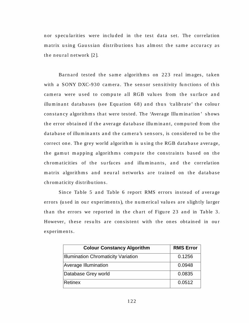
122

nor specularities were included in the test data set. The correlation

matrix using Gaussian distributions has almost the same accuracy as

the neural network [2].

Barnard tested the same algorithms on 223 real images, taken

with a SONY DXC-930 camera. The sensor sensitivity functions of this

camera were used to compute all RGB values from the surface and

illuminant databases (see Equation 68) and thus ‘calibrate’ the colour

constancy algorithms that were tested. The ‘Average Illumination’ shows

the error obtained if the average database illuminant, computed from the

database of illuminants and the camera’s sensors, is considered to be the

correct one. The grey world algorithm is using the RGB database average,

the gamut mapping algorithms compute the constraints based on the

chromaticities of the surfaces and illuminants, and the correlation

matrix algorithms and neural networks are trained on the database

chromaticity distributions.

Since Table 5 and Table 6 report RMS errors instead of average

errors (used in our experiments), the numerical values are slightly larger

than the errors we reported in the chart of Figure 23 and in Table 3.

However, these results are consistent with the ones obtained in our

experiments.

Colour Constancy Algorithm RMS Error

Illumination Chromaticity Variation 0.1256

Average Illumination 0.0948

Database Grey world 0.0835

Retinex 0.0512

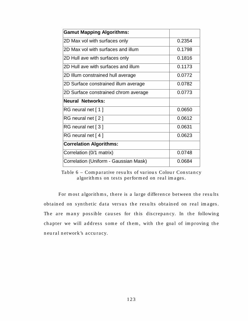
123

Gamut Mapping Algorithms:

2D Max vol with surfaces only 0.2354

2D Max vol with surfaces and illum 0.1798

2D Hull ave with surfaces only 0.1816

2D Hull ave with surfaces and illum 0.1173

2D Illum constrained hull average 0.0772

2D Surface constrained illum average 0.0782

2D Surface constrained chrom average 0.0773

Neural Networks:

RG neural net [ 1 ] 0.0650

RG neural net [ 2 ] 0.0612

RG neural net [ 3 ] 0.0631

RG neural net [ 4 ] 0.0623

Correlation Algorithms:

Correlation (0/1 matrix) 0.0748

Correlation (Uniform - Gaussian Mask) 0.0684

Table 6 – Comparative results of various Colour Constancyalgorithms on tests performed on real images.

For most algorithms, there is a large difference between the results

obtained on synthetic data versus the results obtained on real images.

The are many possible causes for this discrepancy. In the following

chapter we will address some of them, with the goal of improving the

neural network’s accuracy.

124

Chapter 8

Theory versus Praxis: Improving the Theoretical Model

8.1 Modelling specular reflections

In the experiments presented in the previous chapters, we used a

simplified data model, in which we assume that the surfaces are matte,

that there is only one uniform illuminant in the scene and that the

imaging device is perfect. In this ideal world, the performance of the

neural network was very good, but when tested on real images, the

accuracy of illuminant estimates decreased significantly. The same

degradation in accuracy could be seen for the other colour constancy

algorithms, as well. This shows that the images are quite different than

our simplified model, and that more imaging aspects must be taken in

account.

We believe that we can obtain more accurate illuminant estimates

if we use a more precise model for the data used to train the neural

network. Therefore, in this chapter we will extend the model used to

generate the data for the neural network. We will assume that not all

surfaces are matte, some containing specular reflections, and that they

also contain a certain amount of noise (Cardei et al., 1997).

With the exception of Lee’s and Tominaga’s colour constancy

algorithms (Lee, 1986; Tominaga, 1997), which estimate the illuminant

based on the specular reflections present in the image, most other

approaches to colour constancy do not take specularities into account.

As expressed by the equations of the dichromatic model of reflection (see

Equations 30 and 31 in chapter 5.6), the light reflected from a surface is

125

an additive mixture of a specular and a body component. The colour of

specular reflections is virtually independent of the surface reflectance

and has the colour of the illuminant. Therefore, the specular component

of reflection produces a colour shift from the surface colour (as seen

under the scene illuminant) to the colour of the illuminant, as shown in

Figure 5 in Chapter 5.6 and illustrated in Figure 32, below:

Figure 32 –An example of a real image, with and without specularreflections.

In the image above, the specularities were almost totally

eliminated by using a linear polarizing filter. The amount of polarisation

of the specular reflections depends on the incidence angle; for an angle

larger than Brewster’s angle, the specular reflected light is totally

polarized and can be filtered out. However, in the general case, the

incidence angle varies for the surfaces in the image and therefore

specularities must be taken into account.

Because the performance of the neural network is related to the

accuracy of the theoretical model that is used to train it, we modified the

training set to include random amounts of specularity based on the

126

dichromatic model of reflection (Shafer, 1985), discussed in chapter 5.6.

This was done by adding a random amount of scene illumination

(RGBIllum) to the matte RGB component of the synthesized surface

colours:

⋅+

=

′′

Illum

Illum

Illum

BGR

rBGR

BGR

(73)

Each scene was generated by selecting n surfaces at random and

computing their RGB values, to which we added a random amount r of

the scene illumination. The value of r for a scene i was computed as the

product between the maximum value of the specular component S and a

random, sub-unitary coefficient p:

pSri ⋅= (74)

S is the maximum specular brightness allowed in the image, and

ranges from 0% (i.e. no specularities at all) to 100% (i.e. a glossy

surface). Since surface specularities are not uniformly distributed in real

images, we also created a non-uniform distribution of p by squaring a

uniformly distributed random function:

2()rndp = (75)

This model has an expected value for the specular coefficient p of

33.3% and a standard deviation of 29.81%, which assures that generally

only a few surfaces in the scene are highly specular. However, this

distribution might not correspond to the real distribution of specular

127

reflections in an image. All surfaces in the scenes also contain a random

amount of white noise of maximum ±5% of the RGB values.

8.2 The experimental setup

We experimented with two different architectures of multilayer

Perceptrons with two hidden layers. The first neural network is a ‘3600–

200–50–2’ network, identical to the one used in the previous chapter, on

tests done on real images. We used the same network to show the

improvement obtained by using specularities in the training set. The

second neural network is a ‘2500–400-30-2’ network. The error measure

that we used was the Euclidean distance in the chromaticity space

between the target output (illuminant) and the estimated one, the same

error as the one used in previous experiments.

Both networks were trained on large training sets containing

synthesized scenes. Each training set consists of 8900 artificially

generated scenes (100 scenes for each of the 89 illuminants). Each scene

was generated by randomly selecting a number n of surfaces (ranging

from 10 to 100) from the surface reflectance database (which contains

260 surface reflectances) and integrating them with an illuminant picked

at random from the illuminant database (89 illuminants) and the three

SONY camera sensors. To these values, we added a random amount r of

the scene illumination, as described in the previous sections.

We generated training sets with different amounts of maximum

specularity (ranging from 0% to 100%) and trained the networks for 10

epochs on each training set. All networks of the same architecture were

trained starting from the same initial, untrained network. This assured

that the training depends only on the training sets and not on the initial

128

random values of the networks. In the end, we obtained one neural

network for each training set.

The average estimation errors obtained by the neural networks

ranged for the training sets from 0.83% to 1.1%. When tested on newly

artificially generated scenes, these errors increased to 1.2% to 1.5%.

8.3 Results on real images using the improved theoretical model

All neural networks were tested on the same set of 48 real images

used to test the network in the previous chapter. The results are

presented in Table 7 and Table 8:

Specularity (%) Mean

Error

Std.

Dev.

Improvement (%)

0% 0.059 0.043 —

5% 0.051 0.035 13.5%

10% 0.044 0.026 25.4%

25% 0.044 0.032 25.4%

>50% ≈0.044 ≈0.035 25.4%

Table 7 – Experimental results for the ‘3600–200–50–2’ network

Specularity (%) Mean

Error

Std.

Dev.

Improvement (%)

0% 0.057 0.047 —

5% 0.051 0.037 11.3%

10% 0.055 0.038 3.4%

25% 0.049 0.036 13.9%

50% 0.046 0.032 19.1%

Table 8 – Experimental results for the ‘2500–400–30–2’ network

129

Table 9 presents results for the ‘3600–200–50–2’ network obtained

with a specular model containing at most 25% specular reflections

(S=25%). This network has the same architecture as the network that

was used in the previous chapter in the tests on real images. The errors

(in row #7) show that modelling specular reflections improved the

performance of the neural network by around 25%. Statistical

significance tests comparing the two neural network models yield a

confidence level of 94.1%.

# Method Mean σ ∆Lab

1 Illumination chromaticity variation .090 .062 22.38

2 Grey World (GW) .071 .051 15.27

3 Retinex (WP) .075 .049 16.36

4 Neural Network .059 .043 15.03

5 2D gamut mapping using surface

constraints only

.054 .047 12.90

6 2D gamut mapping using surface

and illumination constraints

.047 .039 12.67

7 Neural Network with 25%

specularity model

.044 .032 12.13

Table 9 – Improvement of a neural network’s accuracy trained onsynthetic scenes containing specularities, versus other colour constancy

algorithms when tested on real images.

The neural network trained on scenes with specular reflections

also obtained more accurate estimates of the illumination chromaticity

than any of the other methods tested, which indicates that a theoretical

model that is closer to reality yields more accurate illuminant estimates.

130

On the other hand, it is rather hard to determine the amount of

specularities on which to train the network because this depends only on

the specularities present in the real images, which, in turn, depend on

the physical properties of the surfaces. Since we do not know this

amount a priori, we can not design a “universal” training set. Still, by

training on larger sets, with a larger variety of specularities, the results

can be further improved.

Moreover, much of the difference in error obtained for tests on real

versus synthesized scenes, from around 0.044 to around 0.010, remains

unaccounted for, even when using the specular model in the training set.

In the next chapter we will show that by training on data extracted from

real images, the estimates of the neural networks can be further

improved.

131

Chapter 9

Colour Constancy in Natural Scenes

9.1 Training on Real Images

As shown in the previous sections, even complex theoretical

models can not compensate for much of the difference in accuracy

between tests done on synthesized images versus real ones. Therefore, to

further improve the performance of our neural network approach to

colour constancy, we had to take the training process a step further and

train on data derived from real images and not from images synthesized

according to some mathematical model.

Using images instead of synthetic data for training has the some

advantages. First, it provides the neural network with an accurate RGB

distribution that is to be expected in the test images. During training on

synthetic data, all surfaces and illuminants were considered equally

probable, which is not necessarily true in the real world. This pre-

supposition lead to a certain RGB distribution in the training sets.

Training on real images eliminates this arbitrary uniform distribution in

favour of a distribution that is close to the real one. Second, all image

artefacts, such as specularities and noise, are built-in the image RGBs,

and do not have to be taken separately into account. And third, it

eliminates the need for careful camera calibration (Barnard et al., 1999).

On the other hand, training on real data posed new challenges.

The main problem that we faced with training on real images was to

obtain a sufficiently large number of images. Since obtaining 10,000 or

more images is not practical, we had to find a different solution. Thus,

132

we created new image histograms from subsets of the pixels present in

the original real images. We experimented with training sets that were

actually generated from only 44 images. This sub-sampling approach

solves the problem of generating a large number of scenes, but it

inherently limits the network’s ‘life experience’ to a small set of images,

that might be more or less representative. The images used for training

and testing the neural network were taken with a Kodak DCS460 digital

camera. They contain outdoor scenes, taken in daylight at different times

of day, as well as indoor scenes, taken under a variety of tungsten and

fluorescent light sources as well as with coloured filters.

Another difficulty posed by training on real images is that the

actual scene illumination must be carefully measured in each image. The

chromaticity of the light source in each scene was determined by taking

an image of a reference white reflectance standard in the same

environment. The average distance ∆ELab in the CIE LAB space between

the chromaticity of a light source and the reference white was 14.3 and

the maximum distance was 40.

To obtain even more training and test data, all images were

downloaded from the camera using two different camera driver colour

balance settings (‘Daylight’ and ‘Tungsten’). These settings perform a pre-

defined colour correction. However, the images were not properly colour

balanced, since the actual illumination under which the images were

taken was usually different from either of those two settings of the

camera. We made no assumptions regarding the camera sensors, nor

about the two colour balance settings of the camera driver. We measured

the gamma of the camera, and found it to be approximately equal to 1.6,

so we linearized the images accordingly.

133

The neural network was trained for five epochs on data derived

from the 44 real images. Each image was pre-processed in the same way

as for training on synthetic data; dark, clipped and noisy pixels were

ignored. The set of chromaticities appearing in each of the 44 pre-

processed images was then randomly sampled to derive a large number a

training images. A total of 50,000 scenes, each containing from 10 to 100

distinct chromaticities, were generated in this way from the input images

to form a large training set. We also trained a similar neural network on

a synthetically generated training set.

The results that we report here were obtained with neural

networks of type ‘3600–400–40–2’. The test set contains 42 real images,

different from the ones used for training. Table 10 illustrates the

performance of the neural network relative to other colour constancy

algorithms. The mean error and standard deviation σ are computed in

the rg-chromaticity space. Average errors in the CIE Lab space are also

reported. The relative accuracy (α) represents the ratio of the average

error of a colour constancy algorithm relative to the neural network.

Method Mean σ ∆ΕLab α

Illumination chromaticity variation 0.1484 0.0438 43.21 11.41

Grey World algorithm 0.0556 0.0370 11.26 4.27

White-Patch algorithm 0.0486 0.0365 11.25 3.73

Neural Network trained on

synthetic scenes

0.0355 0.0278 7.98 2.73

Neural Network trained on natural

scenes

0.0130 0.0079 3.77 1.00

Table 10 – Results obtained on tests performed on natural images.

134

The neural network trained on natural scenes has an average

estimation error that is only 36% of that of the neural network trained on

synthesized scenes and is very close to the performance on theoretical

data.

9.2 An Example of Colour Correction

Figure 33 shows an example of colour correction, using different

colour constancy algorithms. After estimating the illuminant, the image

is corrected using the diagonal model (Finlayson et al., 1994, 1994a).

Because all three colour channels are being scaled during colour

correction, the brightness of individual pixels is also changed in this

process. This is why, after applying the diagonal transformation, the

brightness of the pixels is adjusted globally, such that the average image

brightness remains constant.

Figure 33a shows the original image, taken under an unknown

illuminant. Figure 33b shows the target image, taken under the

canonical illuminant. The goal of the colour constancy algorithms we

tested is to estimate the illuminant under which the image in Figure 33a

was taken, such that the original image can be transformed into an

image as close as possible to the one in Figure 33b. Figure 33c shows the

result obtained using a neural network. For this image, we used a neural

network of type ‘3600— 400–50–2’. Figure 33d shows the results of the

gamut mapping algorithm (Finlayson, 1995). Figure 33e shows the

image obtained when using the white patch (WP) algorithm, while Figure

33f shows the image obtained when using the grey world (GW) algorithm.

Excellent results were obtained on real data with a network trained

on real image data by sub-sampling only a few images in order to create

135

a large enough training set. The average ∆ELab error is small (less than

5) and compares favourably with that obtained by human subjects in

Brainard’s experiments (Brainard, 1997).

Figure 33 – Example of colour correction, using different colourconstancy algorithms.

136

Chapter 10

Bootstrapping Colour Constancy

As we have seen in the previous chapters, the quality of the data

used for training the neural networks is crucial for their accuracy. We

generated this data in two ways: either synthesised from databases of

measured reflectances and illuminants or derived from real images by

the sub-sampling method described in the previous chapter.

Both methods have advantages and disadvantages. Synthesizing

scenes from databases of reflectances and illuminants has the advantage

that a large number of scenes can be easily generated and that the

environment is completely controlled. On the other hand, to synthesise

scenes, the spectral sensitivity functions of the camera must be known

and other artefacts (e.g. noise, specularities, camera non-linearity, flare,

etc.) that are unavoidable in real images must also be taken into

account. Another disadvantage is that the colour distribution in the

synthetic scenes might not be consistent with the real world distribution

and can therefore have a negative impact on the network’s accuracy.

Generating training data from real images has the advantage that

the colour distribution is close the real world distribution (as far as the

images used for training are representative of the real world) and that all

image artefacts are built in the training data itself and need not be taken

separately into account. Moreover, it is not necessary to know the

camera sensor sensitivity functions. On the other hand, using real data

requires a large set of images for which the actual illuminant has been

measured.

137

The bootstrapping algorithm (Funt et al., 1999) that is presented in

this chapter addresses both problems: it uses real images to generate the

training data sets and, at the same time, eliminates the need for

illuminant measurements.

10.1 The bootstrapping a lgorithm

The bootstrapping algorithm refers to the method by which the

data sets used for training are generated from real images. Consider a set

of images taken under a number of unknown illuminants with an

uncalibrated camera (i.e. a camera with unknown sensor sensitivities).

Instead of measuring the actual illuminant in the images used to

produce the training set, we use the illuminant estimates given by a

simple colour constancy algorithm. In our experiments, we used the grey

world algorithm, described in detail in chapter 5. This algorithm is quite

accurate if there are enough surface colours in the image. Therefore, we

make the assumption that the images have a relatively large number of

colours. This assumption is easy to verify for each image used for

producing the training set.

For each image, the grey world algorithm gives an estimation of the

illuminant. Each image is then sub-sampled, and a large number of

scenes is generated. The illuminant in all scenes derived from an image

is the one estimated by the grey world algorithm for that image.

Therefore, when a neural network is trained on these scenes, it receives

the grey world algorithm’s estimate of the illumination chromaticity

instead of the actual illuminant. Thus, we are able to train on a large

data set derived from real images without knowing the actual illuminant

of the images.

138

At first glance–from a neural network perspective–the training

process (which, in our experiments, uses the backpropagation algorithm

to tune the network’s weights and thresholds) is considered to be

supervised (Reed et al., 1999) because the network’s output values are

compared with a set of known target values and the network’s

parameters are updated such that the difference between the actual and

target output values is minimised with respect to some metric. However,

the bootstrapping algorithm does not provide accurate target values, but

only more or less accurate estimates computed using the simple grey

world algorithm. In this respect, the bootstrapping algorithm (which

includes the neural network training) can be considered a self-supervised

learning method. Please note that although the bootstrapping algorithm

is self-supervised, the neural network training process itself remains

supervised, since the network is provided with target values, albeit

imperfect ones.

We tested this algorithm both on a very large number of artificial

images generated from a database of 100 illuminants and 260 surface

reflectances and on real images taken with a digital camera. Although

trained with inexact target values, the neural network is more accurate

than the GW algorithm that was initially used to train it, especially for

scenes with a small number of surfaces.

10.2 Bootstrapping experiments on synthetic data

The goal of the experiments performed on synthetic data is to

validate the bootstrapping algorithm in a completely controlled

environment. The input data to the neural network is a training set

composed of 10,000 images and the estimates of the corresponding

139

illuminants provided by the GW algorithm. The network sub-samples

these images into a larger set of 100,000 scenes. Each scene is generated

by choosing a random number of surfaces from one of the input images.

The minimum number of surfaces per scene was set to 10, while the

maximum was given by the actual number of surfaces in the input

images. Thus, if the number of surfaces in the synthetic images is equal

to 35, the sub-sampled scenes have from 10 to 35 surfaces. In the case

of a scene composed of 35 surfaces, the whole image is passed to the

network. In a second experiment, where we generated synthetic images

composed of 50 surfaces per scene, the network was trained on scenes

composed of 10 to 50 surfaces per scene.

The illuminant of each sub-sampled image is inherited from the

synthetic image from which it was generated. Thus the grey world

algorithm bases its estimate on the full image, while only the sub-

sampled image is passed to the network. As a result, the grey world

estimate is more accurate and more stable than it would be if it were

computed on only the sub-sampled data. The networks are trained for

ten epochs on a set of scenes for which the illuminant is not known

exactly. Even so, the average error drops quickly to around 0.015, which

is a satisfactory value.

In order to compare the bootstrapping algorithm to previous

experiments done on synthetic scenes, where the network was trained

with exact illuminant values, we also generated a separate training set of

100,000 scenes, composed of 10 to 50 surfaces each, for which the exact

illuminant values were provided to the network. In all other respects, the

network was trained in the same way as before.

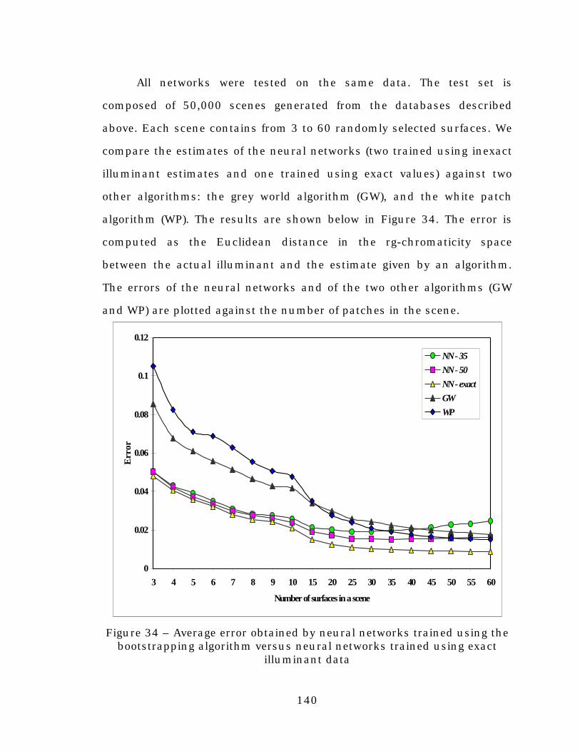
140

All networks were tested on the same data. The test set is

composed of 50,000 scenes generated from the databases described

above. Each scene contains from 3 to 60 randomly selected surfaces. We

compare the estimates of the neural networks (two trained using inexact

illuminant estimates and one trained using exact values) against two

other algorithms: the grey world algorithm (GW), and the white patch

algorithm (WP). The results are shown below in Figure 34. The error is

computed as the Euclidean distance in the rg-chromaticity space

between the actual illuminant and the estimate given by an algorithm.

The errors of the neural networks and of the two other algorithms (GW

and WP) are plotted against the number of patches in the scene.

0

0.02

0.04

0.06

0.08

0.1

0.12

3 4 5 6 7 8 9 10 15 20 25 30 35 40 45 50 55 60

Number of surfaces in a scene

Err

or

NN - 35NN - 50NN - exactGW WP

Figure 34 – Average error obtained by neural networks trained using thebootstrapping algorithm versus neural networks trained using exact

illuminant data

141

The results show that, even when trained with inexact illuminant

chromaticity values in the training set (provided by the grey world

algorithm), the neural network still makes better estimates of the

illumination’s chromaticity in the test scenes. Even more interesting, it

exhibits a ‘bootstrapping’ characteristic, yielding better results than the

grey world algorithm which was used to train it, especially on images

with few colours. For 35 or fewer surfaces in a scene, all neural networks

yield more accurate estimates than the GW and WP algorithms.

The neural network that was trained on exact data (NN-exact

shown in Figure 34) performs consistently better than GW and WP even

on larger numbers of surfaces per scene. The neural network (NN-35)

that was trained on scenes composed of maximum 35 surfaces and on

illuminant estimates provided by GW is surpassed by the GW and WP

algorithms for scenes with more than 35 surfaces. This happens for two

reasons. First, both GW and WP converge to almost zero estimation error

as the number of surfaces in the scene approaches the number of

surfaces in the database. Second, the neural network performs slightly

worse on scenes containing more surfaces than it ever encountered

during training (35 in this case).

Similar results, although not as distinct, occur in the case of the

neural network (NN-50) trained on scenes with a maximum 50 surfaces

and on illuminant estimates provided by GW. This network is also

surpassed by both GW and WP algorithms for scenes with more than 50

surfaces.

142

10.3 Bootstrapping experiments on real images

The successful experiments on synthetic data proved the validity of

the bootstrapping algorithm. The next step tests the bootstrapping

algorithm on real images, because it is for real images where this

algorithm is most useful.

For the experiments done on real images we used images of

natural scenes taken with a Kodak DCS460 digital camera. The original

resolution of 2,000-by-3,000 pixels was reduced to around 1,000-by-600

for all images. We divided the images into two sets, one to be used for

training and the other for testing. The images were linearized to

compensate for the camera built-in gamma correction, but otherwise we

did not make any other assumptions regarding the data. To remove part

of the noise and to reduce the resolution, the images were also

resampled. The chromaticities of the actual illuminants were measured

using a standard white patch in the images. However, this white patch

was eliminated in the images, since it would otherwise bias the results

obtained by the WP algorithm, which partially relies on the presence of a

white patch in the image. The database average used to compensate the

GW algorithm was computed by averaging all surface RGBs in the

images. Although it does not provide a perfect compensation, as it does

with the synthetic data where the surface distribution is known in

advance, it does improve the GW illumination estimates. The results of

experiments done on real images show the positive effect of the database

compensation.

We used 47 images for training. Each image was sub-sampled into

a number of scenes containing from 10 to 300 randomly selected pixels

from the original images. The illuminant corresponding to these scenes

143

was inherited from the estimation provided by the GW algorithm which

computed the illuminant based on the entire image. A second neural

network was trained on exact illuminant feedback. A total of 47,000

scenes were generated (1,000 scenes from each image) for the training

set. Both networks were trained separately for 10 epochs.

In the experiment done on real images, we tested both neural

networks on 39 images. We compared the ‘bootstrapped’ neural network

(i.e. trained on illuminant estimates provided by the GW algorithm) to an

‘exact’ neural network, i.e. a network trained on exact illumination

feedback. Comparisons are also made to the WP and GW algorithms and

the ‘Illumination Chromaticity Variation’ (ICV). ICV measures of the

average shift in the rg-chromaticity space between a chosen canonical

illuminant and the correct illuminants. In our experiments, the canonical

illuminant was selected to be the one for which the CCD camera was

balanced; i.e. the illuminant for which the image of a standard white

patch records identical values on all three RGB colour channels.

The results are shown below in Table 11. The mean error

represents the average estimation error over all images. The standard

deviation is also shown. Both neural networks perform much better than

the other colour constancy algorithms. The GW algorithm with database

compensation has a small average error, too. However, in the general

case, where the statistics of the surfaces are not known a priori (see ‘grey

world without database compensation’ in Table 11), the results of the GW

algorithm are worse, comparable to those of the WP algorithm.

144

Colour Constancy Algorithm Mean Error Std. Dev.

Illumination Chromaticity Variation (ICV) 0.1239 0.0632

Grey World without database compensation 0.0862 0.0440

Grey World with database compensation 0.0471 0.0340

White Patch 0.0847 0.0483

Bootstrapped Neural Network 0.0389 0.0179

Exact Neural Network 0.0222 0.0293

Table 11 – Estimation accuracy of a bootstrapped versus an ‘exact’neural network and other colour constancy algorithms, tested on real

images.

The network ‘learns’ to make a better estimate than the simple grey

world algorithm used in initially training it. This substantially simplifies

the effort required to obtain or synthesise the training set. This approach

works even if the camera sensors are unknown, thus providing an easy

way for colour correcting images taken with an uncalibrated camera. On

the other hand, the accuracy of the ‘bootstrapped’ neural network is not

as good as the accuracy of a network trained on exact illuminant

chromaticities.

The figure below shows an example of colour correction using a

neural network that was trained with the bootstrapping algorithm. The

images in the collage are produced based on the estimates given by the

Grey World algorithm, a neural network trained on accurate illuminants

and a bootstrapped neural network.

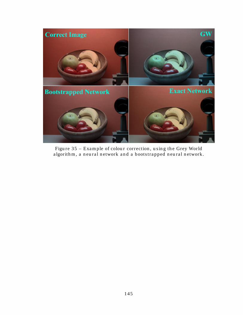
145

Figure 35 – Example of colour correction, using the Grey Worldalgorithm, a neural network and a bootstrapped neural network.

146

Chapter 11

Colour Correcting Images of Unknown Origin

Colour correcting images of unknown origin (e.g. downloaded from

the Internet, scanned from various types of film, etc.) adds additional

challenges to the already difficult problem of colour correction, because

neither the pre-processing the image was subjected to, nor the camera

sensors or camera balance are known. In this chapter, we address these

problems and propose a general framework for dealing with the issues

raised by this type of images. In particular, we discuss the issue of colour

correction of images where an unknown ‘gamma’ non-linearity may be

present. We show that the diagonal model used for colour correcting

linear images also works in the case of gamma corrected images. In the

last part of the chapter, we discuss the influence that unknown sensors

and unknown camera balance has on colour constancy algorithms

(Cardei et al., 1999b, 1999c).

Existing colour constancy algorithms rely in one way or another on

a calibrated camera as well as on assumptions about the statistical

properties of the expected illuminants and surface reflectances.

Therefore, estimating the illumination chromaticity in images of

unknown origin poses new challenges. First, not knowing the sensor

sensitivity curves of the camera means that even for a known surface,

seen under a known illuminant, we are not able to compute its RGB

values.

Figure 36, illustrates how much the chromaticities in the

rg-chromaticity space can vary between cameras. It shows the rg

chromaticities of the Macbeth Colorchecker patches that would be

147

obtained by a SONY DXC-930 and a Kodak DCS460 camera, both colour

balanced for the same illuminant (i.e. both cameras yield the same

R=G=B pixel values for a standard white patch seen under that

illuminant). The data in Figure 36 was synthesised from the known

camera sensor sensitivities, in order to avoid that the values be disrupted

by noise or other artifacts (Cardei et al., 1997). Although the RGB values

for the white and neutral grey patches coincide–as they should, since

both cameras were balanced for the same illuminant–there is a

substantial chromaticity difference between the chromaticities from the

two cameras for many of the other patches.

0.00

0.10

0.20

0.30

0.40

0.50

0.60

0.00 0.20 0.40 0.60 0.80

r

g

DCSSONY

Figure 36 – Variation in chromaticity response of the SONY and Kodakdigital cameras, both calibrated for the same illuminant.

A further problem for colour constancy on images of unknown

origin, is that we do not know the illuminant for which the camera was

balanced. Even if two images are taken with the same camera, the

output will be different for different colour balance settings.

148

Yet another unknown is the camera’s response as a function of

intensity. Cameras often have a non-linear response, the main parameter

of which is often known as the camera’s gamma. For a variety of reasons

(Poynton, 1998), different cameras may have different gamma values or

alternatively may produce linear output (gamma=1). In this paper, we will

use the following definition of camera gamma:

I=SDγ, (76)

where I is the resulting brightness, S is the camera gain, D is a

pixel value in the 0..1 range. A typical value of γ is 0.45, however, the

results below apply for any reasonable value of γ.

Although the chromaticity of white or gray (R=G=B) is preserved, a

change in γ will distort most other chromaticities with the general effect

being to desaturate colours:

++=++=

⇒

++=++=

)/()/(

)/()/(

γγγγ

γγγγ

BGRGgBGRRr

BGRGgBGRRr

gamma

gamma

gamma

(77)

Usually, gammagamma ggandrr ≠≠ .

In the following sections we present a framework for dealing with

each of the above issues related to illumination estimation and colour

correction created by lack of knowledge about a camera’s sensitivity

functions and its γ.

11.1 The effect of γ on co lour correction

In terms of the effect of γ on colour correction, a crucial question is

whether the diagonal model, which has been shown to work well on

149

linear image data (Finlayson et al., 1994), still holds once the non-

linearity of γ is introduced. We address this question both empirically

and theoretically.

Consider an n–by–3 matrix Q1 of RGB values of pixels from an

image seen under illuminant E1 and a similar matrix Q2 containing RGB

values from the same image, but seen under illuminant E2. According to

the diagonal model of illumination change, there exists a diagonal matrix

M such that

21 QMQ =⋅ (78)

It must be noticed that M depends only on illuminants E1 and E2

and does not depend on the pixel values in the images. In particular, if

(R1, G1, B1)wh are the RGB values of white under illuminant E1 and (R2,

G2, B2)wh are the RGB values of white under illuminant E2, then M is

given by

=

12

12

12

/000/000/

GGGG

RRM (79)

For the purpose of this paper, let Mγ denote element-by-element

exponentiation of the elements of matrix M. In the case where the

diagonal model M holds exactly for linear images, then for images to

which a non-linear γ factor has been applied, the diagonal transformation

matrix will become Mγ:

γγγ21

QMQ =⋅ (80)

150

In general, the diagonal model does not hold exactly due to broad

or overlapping camera sensors, so the transformation matrix will also

contain small off-diagonal terms (Worthey et al., 1986). These off-

diagonal terms are amplified by the introduction of γ. To explore the

effects of γ on the off-diagonal terms, we will evaluate the diagonal

transformation between two synthesized images generated using spectral

reflectances of the 24 patches of the Macbeth Colorchecker . One image

is synthesized relative to CIE illuminant A and the other one relative to

D65. We used the spectral sensitivities of the SONY DXC-930 camera

and scaled the resulting RGBs to [0...1].

If A is the matrix of synthesized RGBs under illuminant A and D is

the matrix of RGBs under illuminant D65, the transformation from

matrix D to A is given by:

AMD =⋅ (81)

For linear image data, the best (non-diagonal) transformation

matrix M and the best diagonal matrix MD (in the least square errors

sense) are found to be

=

−−

−=

821.0000036.2000886.3

792.0048.0045.0132.0027.2372.0076.0166.04.225

DM

andM

(82)

These transformation matrices are computed to minimize the mean

square error using the pseudo-inverse:

ADM ⋅= * (83)

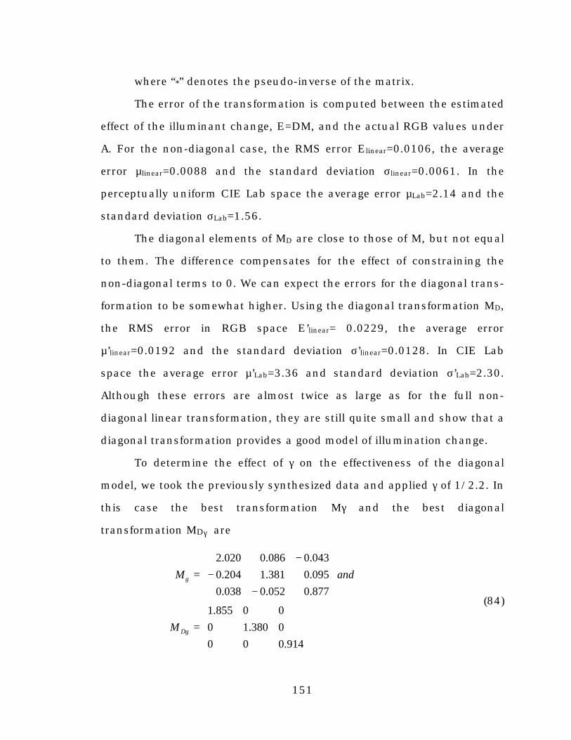
151

where “*” denotes the pseudo-inverse of the matrix.

The error of the transformation is computed between the estimated

effect of the illuminant change, E=DM, and the actual RGB values under

A. For the non-diagonal case, the RMS error Elinear=0.0106, the average

error µlinear=0.0088 and the standard deviation σlinear=0.0061. In the

perceptually uniform CIE Lab space the average error µLab=2.14 and the

standard deviation σLab=1.56.

The diagonal elements of MD are close to those of M, but not equal

to them. The difference compensates for the effect of constraining the

non-diagonal terms to 0. We can expect the errors for the diagonal trans-

formation to be somewhat higher. Using the diagonal transformation MD,

the RMS error in RGB space E’linear= 0.0229, the average error

µ’linear=0.0192 and the standard deviation σ’linear=0.0128. In CIE Lab

space the average error µ’Lab=3.36 and standard deviation σ’Lab=2.30.

Although these errors are almost twice as large as for the full non-

diagonal linear transformation, they are still quite small and show that a

diagonal transformation provides a good model of illumination change.

To determine the effect of γ on the effectiveness of the diagonal

model, we took the previously synthesized data and applied γ of 1/2.2. In

this case the best transformation Mγ and the best diagonal

transformation MDγ are

=

−−

−=

914.0000380.1000855.1

877.0052.0038.0095.0381.1204.0043.0086.02.020

γ

γ

DM

andM

(84)

152

The RMS error using Mγ is Egamma=0.0076 with average error

µgamma=0.0067 and standard deviation σgamma=0.0037. In CIE Lab space

the average error is µγLab=1.06 with standard deviation σγLab=0.69.

For MDγ, the RMS error in RGB space E’gamma= 0.0206, the average

error µ’gamma=0.0180 and the standard deviation σ’gamma=0.0103. In CIE

Lab space the average error µγ’Lab=2.04 with standard deviation

σγ’Lab=1.39. These errors are comparable to the linear case above. These

results indicate that the diagonal model still holds in the case of images

to which a non-linear γ has been applied even in the case where the

diagonal model in the linear case provides only an approximate model of

illumination change.

The above results are summarized in the charts of Figure 37 and

Figure 38. From these charts it is clear that the diagonal model still

holds in the case of images to which a non-linear γ has been applied even

in the case where the diagonal model in the linear case provides only an

approximate model of illumination change. Non-linear errors are smaller

than the linear ones.

0

0.005

0.01

0.015

0.02

0.025

Linear Images Non-Linear Images

RG

B E

rror

Non-Diagonal TransformationDiagonal Transformation

Figure 37 – Error in predicting the effects of illumination change onimage data in RGB space for both linear and non-linear image data.

153

0

1

2

3

4

Linear Images Non-Linear Images

CIE

Lab

Err

or

Non-Diagonal TransformationDiagonal Transformation

Figure 38 – CIELAB ∆ΕLab error in predicting the effects of illuminationchange on image data for both linear and non-linear image data.

Another issue in terms of colour correction of image of unknown γ

has to do with the effects of brightness scaling of the form (R,G,B) to

(kR,kG,kB). A brightness scaling may result either from a change in

incident illumination or camera exposure settings, or it may be applied

as a normalization step during colour correction. In either case, it turns

out that a brightness change does not affect a pixel’s chromaticity even

when γ has been applied.

Consider a pixel (R,G,B) from a linear image with red chromaticity

of r=R/(R+G+B). After γ, its red chromaticity will be

( )γγγγ BGRRr gamma ++= (85)

In the linear case, any brightness scaling leaves the chromaticity

unchanged. In the non-linear γ case, the red chromaticity of a pixel will

be

gammagammaN r)BG/(RR)B)(G)(/((kR)R)(r =++=++= γγγγγγγγ kkk (86)

154

Similar results hold for other chromaticity channels, so brightness

changes do not effect the chromaticities in γ images. Note, however, that

this does not mean that the chromaticity of a pixel is the same before

and after the application of γ.

11.2 Colour correction on non-linear images

We have shown thus far that, whether or not γ has been applied,

the diagonal model works and the brightness of the original image does

not affect the resulting chromaticities. In what follows, we will discuss

the commutativity of γ and colour correction. Given an image I,

represented as an n-by-3 matrix of RGBs, we define two operators on

this image. Γ(I) denotes the application of γ and C(I,M) denotes the colour

correction operator:

( ) γII =Γ (87)

where γ is considered constant, and

( ) MIMIC ⋅=, (88)

We wish to find out if the two operators commute, i.e. if

( )( ) ( )( )MICMIC ,, Γ=Γ (89)

The diagonal transformation matrix M depends on the image I and

the illuminant under which it was taken. This transformation maps

pixels belonging to a white surface in the image into achromatic RGB

pixels (N,N,N).

The problem is that applying γ affects the image chromaticities so a

colour constancy algorithm will receive a different set of input

chromaticities, depending on whether or not the image has had γ applied.

155

Moreover, the diagonal colour correction transformation needs to be

different.

If (Rwh, Gwh, Bwh) is the colour of the illuminant (i.e., the camera’s

response to an ideal white surface under that illuminant) for image I and

(R, G, B) is an arbitrary pixel in I, then

[ ]( )( ) [ ]( ) [ ]γγ

γγ

γγγ

γγγγ BmGmRmMBGRCMBGRC BGR ,,,,,,,, ==Γ (90)

where Mγ is the transformation to be used on the image with

γ applied:

=

B

G

R

m

m

m

M

γ

γ

γ

γ00

00

00

(91)

If we know the colour of the illuminant, the diagonal elements of

Mγ can be computed from the following equation:

[ ]( )( ) [ ]( )[ ] [ ]1,1,1,,

,,,,,,

==

==Γγ

γγ

γγ

γ

γγγγ

γ

whB

whG

whR

whwhwhwhwhwh

BmGmRm

MBGRCMBGRC(92)

Thus, the transformation matrix becomes:

=

γ

γ

γ

wh

wh

wh

BG

RM

/1000/1000/1

(93)

We can rewrite equation 89, as a function of (R,G,B) and (Rwh, Gwh,

Bwh):

[ ]( )( ) [ ]

⋅⋅⋅==Γ γγ

γγ

γγ

γγ

γγ

γγγ B

BG

GR

RBmGmRmMBGRC

whwhwh

BGR 1,1,1,,,,, (94)

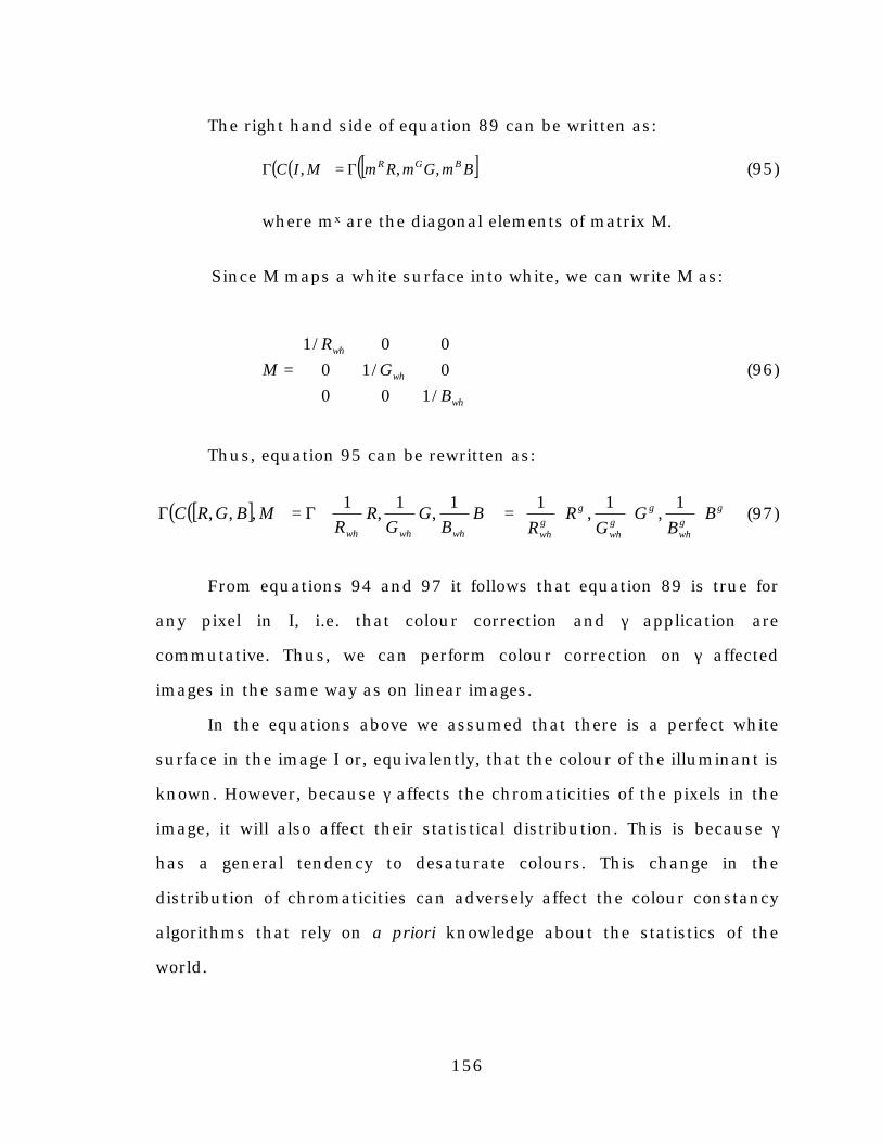
156

The right hand side of equation 89 can be written as:

( )( ) [ ]( )BmGmRmMIC BGR ,,, Γ=Γ (95)

where mx are the diagonal elements of matrix M.

Since M maps a white surface into white, we can write M as:

=

wh

wh

wh

BG

RM

/1000/1000/1

(96)

Thus, equation 95 can be rewritten as:

[ ]( )( )

⋅⋅⋅=

Γ=Γ γ

γγ

γγ

γ BB

GG

RR

BB

GG

RR

MBGRCwhwhwhwhwhwh

1,

1,

11,

1,

1,,, (97)

From equations 94 and 97 it follows that equation 89 is true for

any pixel in I, i.e. that colour correction and γ application are

commutative. Thus, we can perform colour correction on γ affected

images in the same way as on linear images.

In the equations above we assumed that there is a perfect white

surface in the image I or, equivalently, that the colour of the illuminant is

known. However, because γ affects the chromaticities of the pixels in the

image, it will also affect their statistical distribution. This is because γ

has a general tendency to desaturate colours. This change in the

distribution of chromaticities can adversely affect the colour constancy

algorithms that rely on a priori knowledge about the statistics of the

world.

157

11.3 Colour Correcting Images from Unknown Sensors

There are two aspects related to unknown sensors: the colour

balance of the camera and the sensor sensitivity curves. In most cases,

the colour balance is determined by scaling the three colour channels,

according to some predetermined settings. The goal of the colour balance

is to obtain equal RGB values for a white patch under a canonical light.

In this case, we say that the camera is calibrated for that particular

illuminant. Colour correcting images taken with an unknown balance

does not pose a problem, since the calibrating coefficients can be

absorbed in the diagonal transformation that performs the colour

correction.

However, finding the diagonal transformation might prove difficult

for stochastic algorithms that can have difficulties in generalizing their

estimations if they fall outside the illumination gamut for which they

were trained.

If the spectral sensitivity of the sensors of camera that captured an

image is unknown, many colour constancy algorithms will have difficulty

providing reasonable estimates of the scene illumination. In the next

section, we describe tests performed on uncalibrated image data with

several algorithms and found that neural network approaches work quite

well.

11.4 Colour correcting uncalibrated images

We test several different illumination-estimation algorithms on a

database of ‘uncalibrated’ images (the imaging characteristics are not

provided to the algorithms, even though we have the calibration

parameters available so that we can evaluate the results). In particular,

158

we test the white patch algorithm (WP), a version of the grey world

algorithm (GW) and two neural-network-based methods. The gamut-

constraint methods were not tested because they require information

about the expected gamuts of reflectances or illuminants, which can not

be obtained without knowing the sensor sensitivity functions of the

devices that acquired the images.

In the most general case, where the sensors of camera that took an

image are unknown, it is difficult to estimate the scene illumination, due

to the various sensors responses to even the same surfaces under

identical lighting (see Figure 36). In general, imaging devices are

specifically designed to be as close as possible to human colour

perception. Therefore we expect relatively small average colour variations

over the whole image, although such variations can be quite significant

for individual surfaces. For instance, given two images taken under the

same arbitrary light source by two cameras which are calibrated for the

same illuminant, we do not expect to perceive the same surface as green

in one image and as red in the other image.

If the camera sensors are unknown, using a colour constancy

algorithm that has been trained in a self-supervised manner on such

uncalibrated images can provide a simple and effective solution. The

bootstrapping algorithm, presented in the previous chapter, represents a

good choice in this context.

The image database contains 116 images taken with a Kodak

DCS-460 camera and 67 images scanned with a Polaroid Sprintscan 35+

slide scanner from various film types: Kodak Gold, Kodak Royal, Agfa

Optima, Polaroid HiDef and Fuji Superia. The slides were scanned using

a ‘generic’ pre-defined scanner setting. This setting is consistent with the

159

assumption of unknown pre-processing. Using the manufacturer’s

optimal setting for each specific film type would have allowed the scanner

driver to accommodate partially for the differences in film. We divide the

image database into two sets, the first for training and the second for

testing. The training set contains 102 images and is used for training the

neural network and for computing the average colour used in the

database grey world algorithm. The test set contains the other 81 images

(57 DCS images and 24 slides).

Two differently trained neural networks were used for illumination

estimation. The difference between the training of the two networks

concerns the method of determining the actual illuminant. For the first

network, the illuminant chromaticity is simply measured from the

reference white standard that was placed within each image. This

reference white was then eliminated from the images before testing the

colour constancy algorithms.

The second network was trained using the bootstrapping method,

described in the previous chapter. The bootstrapped network uses the

GW algorithm to obtain the chromaticity of the illuminant for the scenes

in the training data. These values, determined by GW, will only be

approximately correct; nonetheless, previous experiments with calibrated

image data showed that the network “learned” to make a better estimate

than the simple GW algorithm used to train it.

The experiments described below show that bootstrapping works

even for the more general case of non-linear images acquired from

various sources. This approach allows us to train a neural network for a

range of uncalibrated cameras and scanners, without having to explicitly

measure white patches in the set of training images.

160

The algorithms were tested on an image database containing 81

images. The charts in Figure 39 and Figure 40 show the relative

performance of the colour constancy algorithms. The figures show the

average errors over the whole test set as well as for each type of input

(i.e. for DCS images and slides). In Figure 39, the average errors are

computed in the rg-chromaticity space, the same space in which the

neural network was trained. “Nothing” refers to assuming that the

illuminant is the one for which the device is calibrated and reflects the

variation in the chromaticity of the illuminant across the test set of

images, relative to white (located at r=g=1/3 in rg-chromaticity space).

“NN” refers to the neural network trained with accurately measured

illumination data, while “Bootstrapped NN” refers to the ‘bootstrapped

neural network.

rg Error

0

0.02

0.04

0.06

0.08

0.1

Nothing GW WP NN Bootstr. NN

DCS ImagesSlidesAverage Error

Figure 39 – Average errors measured in rg-chromaticity space for testsperformed on uncalibrated images.

Figure 40 presents similar results, but with the error measured in

CIE Lab space. The conversion from the RGB space to Lab assumes the

images are viewed on an sRGB-compliant monitor.

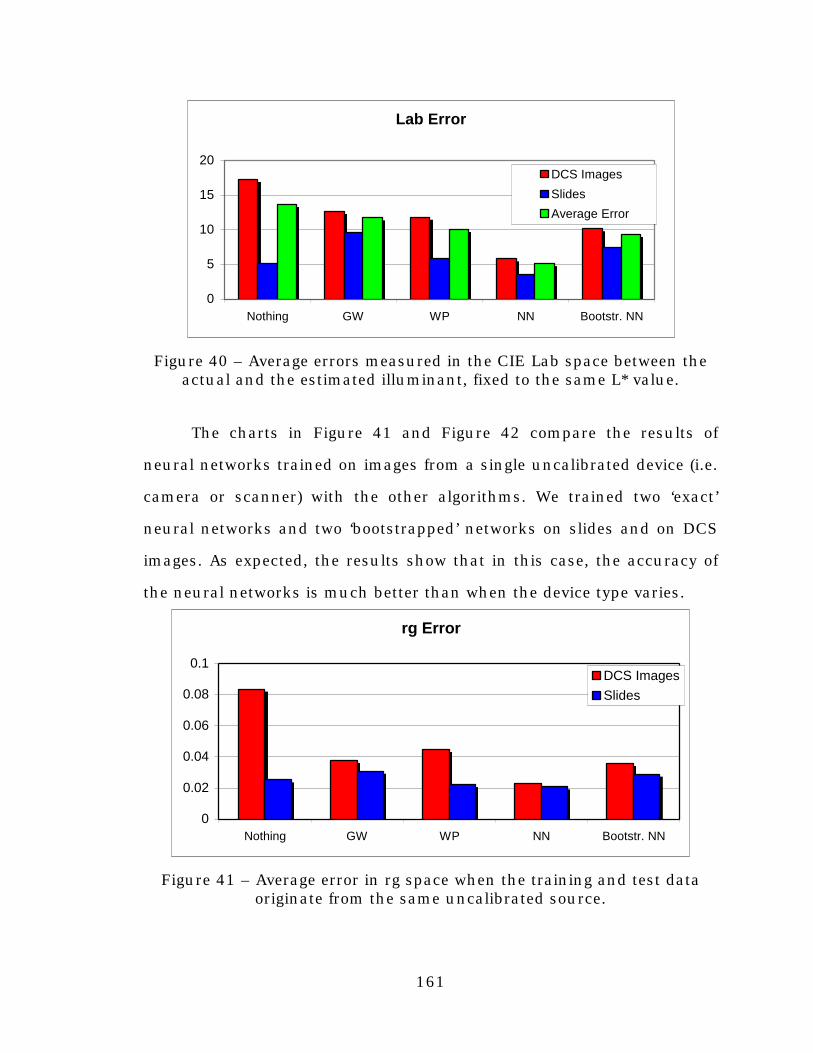
161

Lab Error

0

5

10

15

20

Nothing GW WP NN Bootstr. NN

DCS Images

SlidesAverage Error

Figure 40 – Average errors measured in the CIE Lab space between theactual and the estimated illuminant, fixed to the same L* value.

The charts in Figure 41 and Figure 42 compare the results of

neural networks trained on images from a single uncalibrated device (i.e.

camera or scanner) with the other algorithms. We trained two ‘exact’

neural networks and two ‘bootstrapped’ networks on slides and on DCS

images. As expected, the results show that in this case, the accuracy of

the neural networks is much better than when the device type varies.

rg Error

0

0.02

0.04

0.06

0.08

0.1

Nothing GW WP NN Bootstr. NN

DCS ImagesSlides

Figure 41 – Average error in rg space when the training and test dataoriginate from the same uncalibrated source.

162

Lab Error

0

5

10

15

20

Nothing GW WP NN Bootstr. NN

DCS ImagesSlides

Figure 42 – Average errors measured in the CIE Lab space betweenactual and estimated illuminant fixed to the same L* value when the

training and test data come from the same uncalibrated source.

On this test data, the neural net average error is 5.14∆ELab. We

believe this to be useful for removing colour casts from images of

unknown origin. In the tests with the bootstrapping method of training

the neural network, the ∆ELab error increased to 9.38. Nonetheless, this

is better than either the GW or WP methods. The bootstrapping method

can be applied in situations where accurate measurements of the

illuminant chromaticity are unavailable for training.

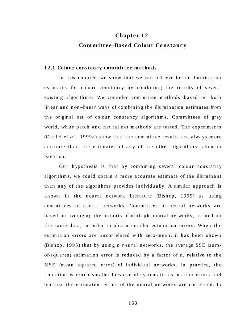
163

Chapter 12

Committee-Based Colour Constancy

12.1 Colour constancy committee methods

In this chapter, we show that we can achieve better illumination

estimates for colour constancy by combining the results of several

existing algorithms. We consider committee methods based on both

linear and non–linear ways of combining the illumination estimates from

the original set of colour constancy algorithms. Committees of grey

world, white patch and neural net methods are tested. The experiments

(Cardei et al., 1999a) show that the committee results are always more

accurate than the estimates of any of the other algorithms taken in

isolation.

Our hypothesis is that by combining several colour constancy

algorithms, we could obtain a more accurate estimate of the illuminant

than any of the algorithms provides individually. A similar approach is

known in the neural network literature (Bishop, 1995) as using

committees of neural networks. Committees of neural networks are

based on averaging the outputs of multiple neural networks, trained on

the same data, in order to obtain smaller estimation errors. When the

estimation errors are uncorrelated with zero-mean, it has been shown

(Bishop, 1995) that by using n neural networks, the average SSE (sum-

of-squares) estimation error is reduced by a factor of n, relative to the

MSE (mean squared error) of individual networks. In practice, the

reduction is much smaller because of systematic estimation errors and

because the estimation errors of the neural networks are correlated. In

164

any case, the average error given by the committee was found to be

smaller than the average of the errors of the individual networks.

In this chapter, we show that a committee of colour constancy

algorithms leads to a better colour constancy. As ‘members’ of the

committee, we used a neural network, similar to those used in our

previous experiments, a version of the white patch algorithm (WP), and

the grey world algorithm (GW).

12.2 Results obtained by colour constancy committees

For our experiments, we used two similar data sets, each

composed of 19,800 illuminant estimates. One, the training set, was

used for optimizing the committees and the other one was used as a test

set for validation. The results reported below are those obtained on the

test set. In a first set of experiments, we compared the individual

performance of the NN, WP and GW algorithms to that of three types of

committees. It should be noted that the NN algorithm has twice the

accuracy of the GW and WP algorithms.

The first type of committee simply averages the outputs of the

three colour constancy algorithms. The individual r and g chromaticity

estimates are averaged, as shown in Equation 98, and the resulting

values rc and gc are compared to the actual illuminant chromaticities.

[ ] [ ]CC

T

WPWPGWGWNNNN grgrgrgr =

⋅

03/103/103/13/103/103/10

(98)

The second type of committee is a weighted average of the outputs

of the individual algorithms. The weights were optimized in the least

mean square (LMS) sense, and were computed from the data available in

165

the training set. The actual values of the weights are shown in Equation

99. It is interesting to notice the cross talk between the red and green

channels (i.e. the influence of the green estimates on those of the red).

[ ] [ ]CC

T

WPWPGWGWNNNN grgrgrgr =

−−−

⋅060.260.0045.041.0113.0675.0150.0015.0040.0018.807.0002.0

(99)

The first two types of committees are linear. It is possible that

there could be some higher-order correlation involved between the

different estimates that are not captured by the linear models. Neural

networks are good at modelling such non-linear statistical properties, so

we experimented with a third type of committee— a neural network (a

multi-layer Perceptron) trained to estimate the illuminant, based on

estimates provided by the other three colour constancy algorithms.

We tried various network architectures and trained each network a

number of times starting from different random initial weights. The

network with the smallest average error over the training set has six

inputs to the neural network, six nodes in a hidden layer and two

outputs nodes. The six input nodes encode the illuminant estimates from

the three algorithms, while the output nodes encode the new

chromaticity estimate. The network was trained on the training set for

50,000 epochs.

166

0.01

0

0.01

5

0.02

0

0.02

5

0.03

0

0.03

5

0.04

0

NN

GW

WP

Mean Average

Simple Committee

LMS Committee

Non-Linear Committee

Figure 43 – The average RMS error of the 3 raw algorithms and thevarious committees.

The average RMS error for each of the original algorithms as well

as the three committees is plotted in Figure 43 where it can be seen that

all three committees result in smaller average errors than the mean error

of the raw colour constancy algorithms (NN, GW and WP) working alone.

The LMS committee provides an 8% improvement over the raw neural

network. Despite the generality of the neural network’s architecture, this

shows that the GW and WP methods still have something additional to

offer when their results are combined with the neural network’s in an

appropriate way. It is interesting to note that the non-linear committee

does not perform as well as the linear LMS committee. This leads to the

hypothesis that there are no higher-order statistical relationships

between the estimates of the raw colour constancy algorithms. Of course,

our failure to find a non-linear network architecture with better

performance does not prove this hypothesis.

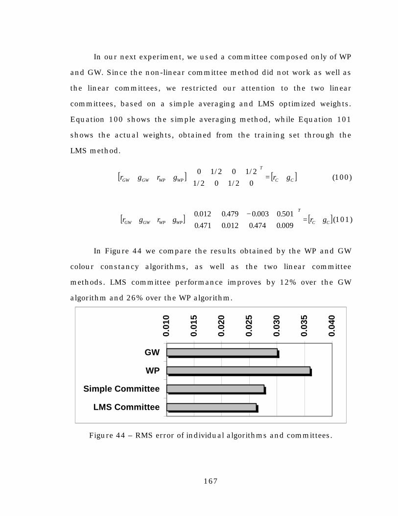
167

In our next experiment, we used a committee composed only of WP

and GW. Since the non-linear committee method did not work as well as

the linear committees, we restricted our attention to the two linear

committees, based on a simple averaging and LMS optimized weights.

Equation 100 shows the simple averaging method, while Equation 101

shows the actual weights, obtained from the training set through the

LMS method.

[ ] [ ]CC

T

WPWPGWGW grgrgr =

⋅

02/102/12/102/10

(100)

[ ] [ ]CC

T

WPWPGWGW grgrgr =

−

⋅009.0474.0012.0471.0501.0003.0479.0012.0

(101)

In Figure 44 we compare the results obtained by the WP and GW

colour constancy algorithms, as well as the two linear committee

methods. LMS committee performance improves by 12% over the GW

algorithm and 26% over the WP algorithm.

0.01

0

0.01

5

0.02

0

0.02

5

0.03

0

0.03

5

0.04

0

GW

WP

Simple Committee

LMS Committee

Figure 44 – RMS error of individual algorithms and committees.

168

Systematic errors in the raw algorithms could adversely affect

committee performance. In particular, GW is prone to systematic errors if

the colours in the test images do not average to the database average

used to compensate for the deviation from grey. To test the effect of

systematic error on the committees, we introduced a systematic shift into

the data set by assuming that the red component of the RGB values of

the surfaces in the test set is 10% higher than its actual value.

This systematically biases the illuminant estimates to be too red.

The actual amount by which the red chromaticity is increased is a

function of pixel brightness and is not necessarily 10%. The new r

chromaticity is given by:

( )BGRRr ++⋅⋅= 1.11.1 (102)

Since the purpose of this test is to test if committees can eliminate

systematic errors, we assumed that WP algorithm is not affected by this

colour shift. Figure 45 shows the performance of two committees, one

employing a simple average and one using a LMS weighted average.

0.01

0

0.01

5

0.02

0

0.02

5

0.03

0

0.03

5

0.04

0

GW

WP

Simple Committee

LMS Committee

Figure 45 – RMS error of individual algorithms and committees. Thesystematic errors introduced in the GW algorithm do not affect the

performance of the LMS committee.

169

The estimation errors of the GW algorithm are larger due to the

systematic estimation error induced by the colour shift described above.

However, the LMS model compensates for the systematic error and yields

the same performance as the model shown in Figure 44.

We have shown that committee models, which combine the results

of two or more colour constancy methods, can significantly improve

overall colour constancy performance. The implementation of these

models is simple and the computational overhead is very small. Thus,

committees provide a useful tool for improved colour constancy.

170

Conclusions

The colour of a surface in an image is determined in part by its

surface reflectance, in part by the spectral power distribution of the light

illuminating it and in part by the camera sensors. Therefore, a variation

in the scene illumination changes the colour of the surface as it appears

in an image. On the other hand, humans exhibit a relatively high degree

of colour constancy and therefore will perceive only a small change, if

any, in the surface colour. Moreover, the colours perceived by human

observers are also influenced by the viewing context and other cognitive

factors. Complex, non-linear colour appearance models emulate most

aspects related to human vision. However, they assume that the colour of

the image illuminant, considered to be uniform in the whole image, is

known.

From a computational perspective, colour constancy algorithms try

to solve this problem and accurately estimate the illumination colour.

This is an underdetermined problem, and in order to solve it, additional

constraints must be added. We have described the most important

classes of colour constancy in Chapter 5 and discussed their advantages

and limitations.

In this thesis we presented a novel approach to colour constancy: a

neural network is used to estimate the chromaticity of the illuminant in a

scene, based only on chromaticities ‘seen’ in that scene by a digital

camera or by other imaging device. We have shown that the neural

network is able to learn colour constancy from synthesised or real data.

We used a neural network instead of a well-defined mathematical

model as an alternative way for solving the colour constancy problem

171

because it is flexible and allows for a dynamic adaptation to a changing

environment. The bootstrapping method shows that a complex colour

constancy algorithm, such as a neural network, can be trained by using

a simple, biologically plausible method, such as grey world. Please note

that we do not claim that the human vision system uses grey world as a

first step to learning colour constancy, nor that the neural network used

for bootstrapping inherits any biological plausibility from the grey world

algorithm.

After an initial series of tests, performed with a ‘standard’

multilayer neural network, we developed and implemented a series of

improvements. Since the gamut of the chromaticities encountered during

training and testing is much smaller than the whole (theoretical)

chromaticity space, we modified the neural network’s architecture, such

that it will receive input only from the active nodes (the input nodes that

were activated at least once). Moreover, due to the fact that the sizes of

the layers are so different, different learning rates were used for each

layer, proportional to the fan-in of the neurons in that layer. These

improvements shortened the training time and increased the estimation

accuracy at the same time.

The neural networks were trained on artificially generated scenes.

Each scene is composed of a variable number of patches seen under one

illuminant, randomly chosen from a database of illuminants. The

patches correspond to matte reflectances, selected at random from a

database of surface reflectances. Therefore each patch has only one rg-

chromaticity, derived from its RGB, which is computed by multiplying a

randomly selected surface reflectance with the spectral distribution of an

illuminant and with the spectral sensitivities of camera sensors.

172

Tests were performed on synthesised scenes as well as on natural

images, taken with a digital camera. Although the performance of the

network was very good when tested on synthetic scenes, the results were

worse on real data. We improved the network’s accuracy by modelling

specular reflections and noise in the training set,

The next step was to train the network on data derived directly

from real images. This approach led to even better results. Although the

networks trained on real images are capable of making accurate

estimates of the scene’s illuminant, the actual illuminant in the images

used to compute the training set must be known with accuracy.

Therefore, the illuminant must be measured for every image used for the

training set.

To overcome this problem, a novel self-supervised training

algorithm, called ‘bootstrapping’, was developed. Grey world illuminant

estimates were used instead of the exact illuminant values for the

training data. Surprisingly, the final performance of the neural network

is better than the performance of the grey world algorithm that was

originally used to train it.

Up to this point, we assumed that we dealt with linear images,

taken with a carefully calibrated camera. The last part of the thesis deals

with the issue of colour correcting images of unknown origin. These are

images taken with unknown cameras or other imaging devices, such as

scanners. Moreover, these images might have been gamma corrected.

This very general aspect of colour constancy encompasses two aspects.

The first aspect is related to the theoretical aspect of colour correction. In

what conditions is it possible to colour correct an image? We have shown

that colour correction (defined as scaling each colour channel by some

173

factor) is possible even for non-linear images, under certain conditions.

The second aspect is related to the problem of determining the illuminant

under which the images were taken. Since the sensor sensitivity

functions and camera balance are unknown, the problem is much more

complicated than in the context were the camera is calibrated. The

experiments we presented prove that a neural network is able to learn

colour constancy even in this very general case.

Using a neural network to estimate the chromaticity of the scene

illumination improved upon existing colour constancy algorithms by an

increase in both accuracy and stability. Subsequent improvements in the

neural network algorithm, such as training on data sets with

specularities, training on real data, bootstrapping the colour constancy

training algorithm, and colour correcting uncalibrated images further

increased the performance of the illuminant estimation.

174

References

M. Anderson, R. Motta, S. Chandrasekar and M. Stokes, “Proposal for aStandard Default Color Space for the Internet – sRGB,” Proc.Fourth Color Imaging Conf., 238-246, 1996.

K. Barnard, “Practical Colour Constancy”, Ph.D. Thesis, Simon FraserUniversity, 1999.

K. Barnard and B. Funt, “Camera calibration for color vision research,”Proc. Human Vision and Electronic Imaging IV, SPIE Conferenceon Electronic Imaging, 576-585, 1999.

K. Barnard, G. Finlayson, and B. Funt, “Color Constancy for scenes withvarying illumination,” Computer Vision and Image Understanding,65(2), 311-321, 1997.

C.M. Bishop, Neural Networks for Pattern Recognition, Clarendon Press,Oxford, 1995.

D. H. Brainard, W. A. Brunt and J. M.. Speigle, “Color constancy in thenearly natural image. 1. Asymmetric matches.” J. Opt. Soc. Am. A,14(9), 2091-2110, 1997.

D.H. Brainard and W.T. Freeman, “Bayesian Color Constancy,” J. Opt.Soc. Am. A, 14(7), 1393-1411, 1997.

D.H. Brainard and B.A. Wandell, “Asymmetric color matching: How colorappearance depends on the illuminant,” J. Opt. Soc. Am. A 9,1433-1448, 1992.

D.H. Brainard and B.A. Wandell, “Analysis of the retinex theory of colorvision,” J. Opt. Soc. Am. A 3, 1651-1661, 1986.

G. Buchsbaum, “A Spatial Processor Model for Object Color Perception,”J. Franklin Institute, 310 (1), 1-26, 1980.

V.C. Cardei and B. Funt, “Color Correcting Uncalibrated Digital Images,”J. of Imaging Science and Technology, Invited Paper. (In Press)

V.C. Cardei and B. Funt, “Committee-based Color Constancy,” Proc.Seventh Color Imaging Conf., Scottsdale, 311-313, 1999a.

V.C. Cardei, B. Funt and K. Barnard, “White Point Estimation forUncalibrated Images,” Proc Seventh Color Imaging Conf.,Scottsdale, 97-100, 1999b.

V.C. Cardei, B. Funt and M. Brockington, “Issues in Color CorrectingDigital Images of Unknown Origin”, CSCS’12, Bucharest, 1999c.

175

V.C. Cardei, B. Funt and K. Barnard, “Adaptive Illuminant EstimationUsing Neural Networks,” ICANN’98, Skövde, Sweden, 749-754,1998.

V.C. Cardei , B. Funt and K. Barnard, “Modeling Color Constancy withNeural Networks,” Proc. Int. Conf. on Vision, Recognition, andAction: Neural Models of Mind and Machine, Boston, 1997.

S. Courtney, L.H. Finkel and G. Buchsbaum, “Network Simulations ofRetinal and Cortical Contributions to Color Constancy,” VisionRes., Vol. 35, No.3, 413-434, 1995.

S. Courtney, L.H. Finkel and G. Buchsbaum, “A Multistage NeuralNetwork for Color Constancy and Color Induction,” IEEE Trans. onNeural Networks, Vol.6, No.4, July 1995a.

A Cowey and C.A. Heywood, “There’s more to color than meets the eye,”Behavioural Brain Research, Vol. 71, 89-100, 1995.

J. Davidoff, Cognition Through Color, MIT Press, Cambridge, Mass.,1991.

S. Dörr and C. Neumayer, "The Goldfish – A Color-Constant Animal,”Perception, Vol. 25, 243-250, 1996.

M.D. Fairchild, Color Appearance Models, Addison-Wesley, 1997.

G. Finlayson, P.M. Hubel and S. Hordley, “Color by Correlation,” Proc.Fifth Color Imaging Conference, 6-11, 1997.

G. Finlayson and S. Hordley, “Selection for Gamut Mapping ColorConstancy,” British Machine Vision Conference, 630-639, Sept.1997.

G. Finlayson, “Color in Perspective,” IEEE Trans. PAMI 18 (10), 1034-1038, 1996.

G. Finlayson, “Color Constancy in Diagonal Chromaticity Space,” IEEEProc. Fifth Intl. Conf. on Comp. Vision, June 20-23, 1995.

G. Finlayson, M. Drew and B. Funt, “Color Constancy: GeneralizedDiagonal Transforms Suffice,” J. Opt. Soc. Am. A, 11(11), 3011-3020, 1994.

G. Finlayson, M. Drew and B. Funt, “Spectral Sharpening: SensorTransformations for Improved Color Constancy,” J. Opt. Soc. Am.A, 11(5), 1553-1563, 1994a.

D.A. Forsyth, “A Novel Algorithm for Color Constancy,” Intl. Journal ofComputer Vision, 5:1, 5-36, 1990.

B. Funt and V.C. Cardei, “Bootstrapping Color Constancy,” Proc. SPIEVol. 3644, Human Vision and electronic Imaging IV, Eds. B.E.Rogowitz and T.N. Pappas, 421-428, 1999.

176

B. Funt, V.C. Cardei and K. Barnard, “Method of Estimating theIlluminant Chromaticity Using Neural Networks,” U.S. Patent5,907,629.

B. Funt, K. Barnard and L. Martin, “Is color constancy good enough?,”5th European Conf. on Computer Vision, 445-459, 1998.

B. Funt, K. Barnard, M. Brockington and V. Cardei, “Luminance-BasedMulti-Scale Retinex,” Proc. AIC Color 97, Vol. I, 330-333, Kyoto,Japan, May 1997.

B. Funt, V.C. Cardei and K. Barnard, “Neural Network Color Constancyand Specularly Reflecting Surfaces,” Proc. AIC Color 97, Vol. II,523-526, Kyoto, Japan, May 1997.

B. Funt, V.C. Cardei and K. Barnard, “Learning Color Constancy,” Proc.Fourth Color Imaging Conf., 58-60, Scottsdale, 1996.

R. Gershon, A.D. Jepson, and J.K. Tsotsos, ”From [R,G,B] to SurfaceReflectance: Computing Color Constant Descriptors in Images,”Perception, 755-758, 1988

J. Hertz, A. Krogh and R.G. Palmer, Introduction to the Theory of NeuralComputation, Addison-Wesley Publishing Company, 1991.

D.H. Hubel and M.S. Livingstone, “Segregation of form, color, andstereopsis in primate area 18,” J. Neuroscience, 7(11), 3378-3415,1987.

D.H. Hubel and T.N. Wiesel , “ Brain Mechanisms of Vision,” ScientificAmerican, Vol. 243, No. 3, 150-162, 1979.

A.C. Hurlbert, “Neural Network Approaches to Color Vision,” NeuralNetworks for Perception. Vol. 1: Human and Machine Perception,266-284, edited by H. Wechsler, Academic Press Inc., 1991.

A.C. Hurlbert and T.A. Poggio, “Synthesizing a Color Algorithm fromExamples,” Science, Vol. 239, 482-485, 1988.

D.J. Jobson, Z. Rahman and G.A. Woodell, “Retinex Image Processing:Improved Fidelity to Direct Visual Observation,” Proc. IS&T/SIDFourth Color Imaging Conference: Color Science, Systems andApplications, 124-126, Scottsdale, Arizona, November 1996.

D.B. Judd, D.C. MacAdam and G Wyszecki, “Spectral Distribution OfTypical Daylight As A Function Of Correlated Color Temperature,”J. Opt. Soc. of Am. A, 54, 1031-1040, 1964.

E.L. Krinov, “Spectral Reflectance Properties of Natural Formations,”Technical Translation TT-439, National Research Council ofCanada, 1947.

E.H. Land, “Recent Advances in Retinex Theory,” Vision Res., 26, 7-22,1986.

177

E.H. Land, “The Retinex Theory of Color Vision,” Scientific American,108-129, 1977.

H. Lee, “Method for computing the scene-illuminant chromaticity fromspecular highlights,” J. Opt. Soc. of Am. A, Vol. 3(10), 1694-1699,1986.

C. Li, M.R. Luo, and R.W.G. Hunt, “The CAM97s2 Model,” Proc. SeventhColor Imaging Conf., Scottsdale, 262-263, 1999.

M.R. Luo and R.W.G. Hunt, “The Structures of the CIE 1997 ColourAppearance Model (CIECAM97s), Color Res. Appl., 23, 138-146,1998.

D.L. MacAdam, Sources of Color Science, MIT Press, Cambridge, Mass.,1970.

L. Maloney and B. Wandell, “Color constancy: a method for recoveringsurface spectral reflectance,” J. Opt. Soc. Am. A, Vol.3, No.1, 29-33, 1986.

R.H. Masland, “Unscrambling Color Vision”, Science, Vol. 271, 616-617,2 Feb. 1996.

J.J. McCann, “Magnitude of Color Shifts from Average-Quanta CatchAdaptation,” Proc. IS&T/SID Fifth Color Imaging Conference: ColorScience, Systems and Applications, 17-22, Scottsdale, 1997.

P.L. Meyer, Introductory Probability and Statistical Applications,Addison-Wesley Publishing Company, 1965

A. Moore, J. Allman and R.M. Goodman, “A Real-Time Neural System forColor Constancy,” IEEE Transactions on Neural Networks, 237-247, Vol. 2, No. 2, March, 1991.

J. Morovic and M.R. Luo, “Gamut Mapping Algorithms Based onPsychophysical Experiment,” Proc. IS&T/SID Fifth Color ImagingConference: Color Science, Systems and Applications, 44-49,Scottsdale, 1997.

A.P. Petrov, “Surface Color and Color Constancy,” Color Res. and Appl.,Vol. 18, No.4, 236-240, August 1993.

D. Plaut, S. Nowlan, and G. Hinton, “Experiments on Learning by BackPropagation,” Technical report, CMU-CS-86-126, Carnegie-MellonUniversity, Pittsburgh, USA, 1986.

C. Poynton, “The Rehabilitation of Gamma,” B.E. Rogowitz and T.N.Pappas (eds.), Proc. of SPIE 3299, 232-249, 1998.

R.D. Reed, R.J. Marks II, Neural Smithing. Supervised learning infeedforward artificial neural networks, MIT Press, Cambridge,1999.

178

D.E. Rumelhart, G.E. Hinton and R.J. Williams, “Learning InternalRepresentations by Error Propagation”, Parallel DistributedProcessing: Explorations in the Microstructure of Cognition.Volume I: Foundations, Eds. D.E. Rumelhart, J.L. McClelland andthe PDP Research Group, 318-362, MIT Press, Cambridge, MA,1986.

S.A. Shafer, “Using color to separate reflection components,” Color Res.Appl., Vol.10, No. 4, 210-218, 1985.

M. Swain and D. Ballard, “Color Indexing,” Int. J. of Computer Vision,7:1, 11-32, 1991.

S. Tominaga, “Surface Reflectance Estimation by the DichromaticModel,” Color Res. Appl., 21, 104-114, 1996.

S. Tominaga, “Separation of Reflection Components from a Color Image,”Proc. Fifth Color Imaging Conf., Scottsdale, 254-257, 1997.

S. Usui, S. Nakauchi and Y. Miyamoto, “A neural network model for colorconstancy based on the minimally redundant colorrepresentation,” Proc. IJCNN (Beijin), vol.2, 696-701, 1992.

J. von Kries, “Chromatic Adaptation,” Festschrift der Albrecht-Ludwig-Universität, Firbourg, 1902. [in D.L. MacAdam, 1970]

J. Walraven and J.W. Alferdinck, “Color Displays for the Color Blind,”Proc. IS&T/SID Fifth Color Imaging Conference: Color Science,Systems and Applications, 17-22, Scottsdale, 1997.

B.A. Wandell, “The Synthesis and Analysis of Color Images,” IEEE Trans.PAMI 9 (1), 2-13, 1987.

B.A. Wandell, Foundations of Vision, Sinauer Associates, Inc., 1995.

B.A. Wandell, H. Baseler, A.B. Poirson, G.M. Boynton and S. Engel,“Computational Neuroimaging: Color Tuning in Two HumanCortical Areas Measured Using fMRI.,” in Color Vision: FromMolecular Genetics to Perception, Eds. K. Gegenfurtner and L. T.Sharpe, Cambridge University Press. (In Press)

J.A. Worthey and M.H. Brill, “Heuristic Analysis of von Kries colorconstancy,” J. Opt. Soc. of Am. A, Vol. 3(10), 1709-1712, 1986.

S.M. Zeki, “The Representation of Colors in the Cerebral Cortex,” Nature,284, 412-418, 1980.

S.M. Zeki, “Color Coding in the Cerebral Cortex. The reaction of Cells inMonkey Visual Cortex to Wavelengths and Colors,” Neuroscience,9, 741-765, 1993.