A Network of Portable, Low-Cost, X-Band Radars

7

A Network of Portable, Low-Cost, X-Band Radars

Marco Gabella1,2, Riccardo Notarpietro2, Silvano Bertoldo3, Andrea Prato2, Claudio Lucianaz3, Oscar Rorato3, Marco Allegretti3 and Giovanni Perona3

1Meteoswiss 2Politecnico di Torino – Electronics Department,

3Consorzio Interuniversitario per la Fisica delle Atmosfere (CINFAI) – Sede di Torino 1Switzerland

2,3Italy

1. Introduction

1.1 Excellent qualitative overview of the weather in space and time

Radar is a unique tool to get an overview on the weather situation, given its high spatio-temporal resolution. Over 60 years, researchers have been investigating ways for obtaining the best use of radar. As a result we often find assurances on how much radar is a useful tool, and it is! After this initial statement, however, regularly comes a long list on how to increase the accuracy of radar or in what direction to move for improving it. Perhaps we should rather ask: is the resulting data good enough for our application? The answers are often more complicated than desired. At first, some people expect miracles. Then, when their wishes are disappointed, they discard radar as a tool: both attitudes are wrong; radar is a unique tool to obtain an excellent overview on what is happening: when and where it is happening. At short ranges, we may even get good quantitative data. But at longer ranges it may be impossible to obtain the desired precision, e.g. the precision needed to alert people living in small catchments in mountainous terrain. We would have to set the critical limit for an alert so low that this limit would lead to an unacceptable rate of false alarms.

1.2 Range dependence of the results (range degradation)

Perhaps accurate quantitative precipitation estimation (QPE) can only be achieved at short ranges from the radar. This is not because we miss careful investigations, but simply, because radar can only see the hydrometeors aloft, while we would need to know what is arriving at ground level. Obstacles as well as earth curvature lead to a limited horizon, allowing us to see precipitation at variable height, often too far from the ground. All these difficulties increase rapidly with range from the radar location. The situation becomes obviously much more difficult in mountainous terrain, where weather echoes can only be detected at high altitudes because of beam shielding by relieves: there, terrain blockage combined with the shallow depth of precipitation during cold seasons and low melting levels causes inadequate radar coverage to support QPE, especially in narrow valleys.

www.intechopen.com

Doppler Radar Observations – Weather Radar, Wind Profiler, Ionospheric Radar, and Other Advanced Applications

176

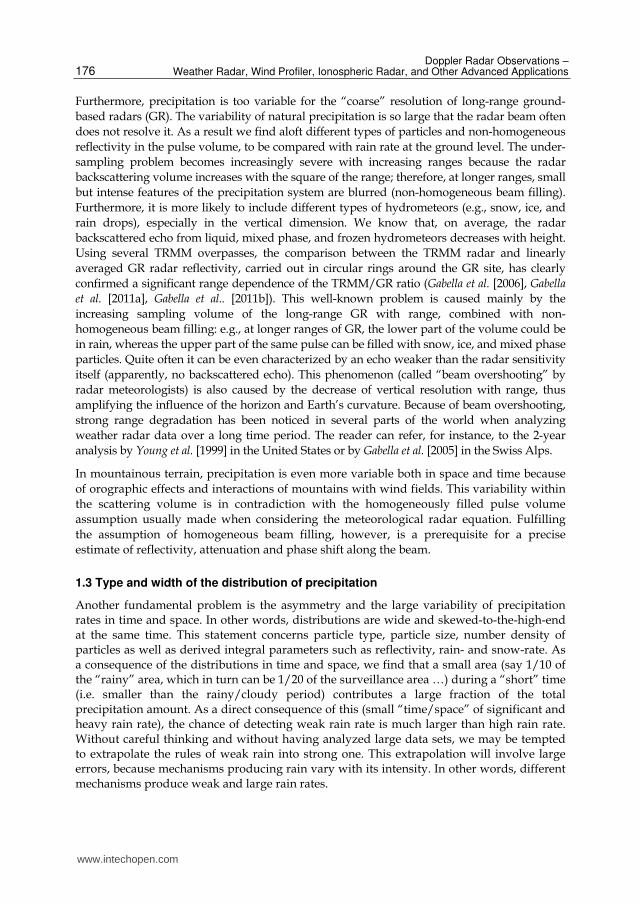
Furthermore, precipitation is too variable for the “coarse” resolution of long-range ground-

based radars (GR). The variability of natural precipitation is so large that the radar beam often

does not resolve it. As a result we find aloft different types of particles and non-homogeneous

reflectivity in the pulse volume, to be compared with rain rate at the ground level. The under-

sampling problem becomes increasingly severe with increasing ranges because the radar

backscattering volume increases with the square of the range; therefore, at longer ranges, small

but intense features of the precipitation system are blurred (non-homogeneous beam filling).

Furthermore, it is more likely to include different types of hydrometeors (e.g., snow, ice, and

rain drops), especially in the vertical dimension. We know that, on average, the radar

backscattered echo from liquid, mixed phase, and frozen hydrometeors decreases with height.

Using several TRMM overpasses, the comparison between the TRMM radar and linearly

averaged GR radar reflectivity, carried out in circular rings around the GR site, has clearly

confirmed a significant range dependence of the TRMM/GR ratio (Gabella et al. [2006], Gabella

et al. [2011a], Gabella et al.. [2011b]). This well-known problem is caused mainly by the

increasing sampling volume of the long-range GR with range, combined with non-

homogeneous beam filling: e.g., at longer ranges of GR, the lower part of the volume could be

in rain, whereas the upper part of the same pulse can be filled with snow, ice, and mixed phase

particles. Quite often it can be even characterized by an echo weaker than the radar sensitivity

itself (apparently, no backscattered echo). This phenomenon (called “beam overshooting” by

radar meteorologists) is also caused by the decrease of vertical resolution with range, thus

amplifying the influence of the horizon and Earth’s curvature. Because of beam overshooting,

strong range degradation has been noticed in several parts of the world when analyzing

weather radar data over a long time period. The reader can refer, for instance, to the 2-year

analysis by Young et al. [1999] in the United States or by Gabella et al. [2005] in the Swiss Alps.

In mountainous terrain, precipitation is even more variable both in space and time because

of orographic effects and interactions of mountains with wind fields. This variability within

the scattering volume is in contradiction with the homogeneously filled pulse volume

assumption usually made when considering the meteorological radar equation. Fulfilling

the assumption of homogeneous beam filling, however, is a prerequisite for a precise

estimate of reflectivity, attenuation and phase shift along the beam.

1.3 Type and width of the distribution of precipitation

Another fundamental problem is the asymmetry and the large variability of precipitation rates in time and space. In other words, distributions are wide and skewed-to-the-high-end at the same time. This statement concerns particle type, particle size, number density of particles as well as derived integral parameters such as reflectivity, rain- and snow-rate. As a consequence of the distributions in time and space, we find that a small area (say 1/10 of the “rainy” area, which in turn can be 1/20 of the surveillance area …) during a “short” time (i.e. smaller than the rainy/cloudy period) contributes a large fraction of the total precipitation amount. As a direct consequence of this (small “time/space” of significant and heavy rain rate), the chance of detecting weak rain rate is much larger than high rain rate. Without careful thinking and without having analyzed large data sets, we may be tempted to extrapolate the rules of weak rain into strong one. This extrapolation will involve large errors, because mechanisms producing rain vary with its intensity. In other words, different mechanisms produce weak and large rain rates.

www.intechopen.com


177

1.4 Difficulties with conventional long-range radar: Inability to observe the lower part of the troposphere combined with non-homogeneous beam filling

We may wonder: why is it so difficult to grasp a realistic precision out of “long-range” (say

two hundred kilometers) weather radar? Perhaps, the main reason can be found in the

difficulty of reproducing the results verified with large effort at close ranges. We cannot

extrapolate them to the full range displayed by our operational, meteorological radars. At

short ranges problems caused by shielding, inhomogeneous beam filling, attenuation and

vertical profile may be dealt with. This is not possible at longer ranges. This statement does

not exclude the use for weather forecasting in full range of our radars. The radar tells us

where and when something is coming; radar data are helpful to validate the forecasts of the

Numerical Weather Prediction models. Here, combining the information of many radars

into a network may help a lot. The combination of data from many radars may also mitigate

the effects caused by the range-dependence of each single radar.

Long-range radar networks remain an essential part of the weather forecasting and warning

infrastructures used by many nations worldwide. Despite significant capability and

continuous improvement, one fundamental limitation of today’s weather radar networks is

the inability to observe the lower part of the atmosphere and detect fine-scale weather

features. Designed for long-range coverage through precipitation, these radars must operate

at radar wavelengths not subject to attenuation. This implies the use of large antennas (to

achieve narrow beam width) and high-power transmitters (to meet sensitivity requirements

at long ranges); up to now, such large antennas are mechanically scanned, hence requiring

dedicated land, towers and other support infrastructures. Consequently, the installation and

acquisition cost of each site is usually much larger than the cost of the sensor itself.

1.5 Proposed solution: Distributed networks of many, inexpensive, redundant, low-cost, high temporal resolution, short-range, small radars

How to tackle the emerging need for improved low-altitude coverage, high temporal-

resolution meteorological radars? Many low-cost, fast-scanning, short-range X-band radars

for rain monitoring can be a valid solution for complementing long-range radars. Long

range radars have proved to be useful for weather forecasting and qualitative surveillance.

As already discussed in Sec. 1.2, the results, verified with large effort at close ranges, cannot

be generalized. Because of range degradation (non uniform beam filling and overshooting,

see Sec. 1.2), it seems impossible to reproduce the results easily obtained close to the radar

for quantitative applications at far ranges. This is especially true in mountainous terrain.

Therefore, an interesting solution could be to combine the data of many, small, low-cost and

short-range X-band radar for rain estimates within valleys.

2. The potential for distributed networks of small low-cost weather radars

2.1 The work of the remote sensing group at the Politecnico di Torino

The European INTERREG IIIB Alpine Space Programme started in 2004 the FORALPS Project (“Meteo-hydrological Forecast and Observations for improved water Resource management in the ALPS”). One of the aims of FORALPS was the design and development of a portable, low-cost, small radar for weather monitoring. The Remote Sensing Group at

www.intechopen.com


178

the Politecnico di Torino was involved in the development activities of this new network starting from its early ideation stages (Notarpietro et al. [2005]).

The first designed scenario was specifically intended to cover narrow valleys within the Alps. This was initially achieved by adopting a non-conventional vertical plane scanning strategy with a fan beam slot waveguide antenna (1° beam width in the vertical plane, 25° beam width along the valley). The initial implementation was simply designed to collect two low elevation acquisitions with opposite directions along the valley plus a vertical sounding to evaluate the vertical reflectivity profile (Gabella et al. [2008]). Then, this initial approach was extended to collect radar sounding coming from the entire vertical plane. This kind of small low-cost radar has been patented and is now sold with the name “wind-mill” mini-radar.

In a second stage, the more conventional horizontal scanning strategy was implemented to cover wide planar areas with very high temporal resolution at a fixed, optimized elevation. This suggested combining a number of short-range, low-cost radars into a network concept, to obtain a set of similar small unattended units, tightly connected within a unified environment. The result of the above approaches and suggestions is an unmaned, low-consumption, network of low-cost, small, X-band radars. Adding up, the first prototypes, running since October 2006, were installed on the Politecnico di Torino roof, sensing either the horizontal or the vertical planes. During these years several progresses and modifications were made, leading to a network of mini radars: one operated by the Aosta Valley Civil Protection (since March 2007) and a vertical scanner unit (wind-mill) installed next to the glide path of the “Sandro Pertini” Turin International Airport. Recently (autumn 2010), four horizontal scanners units were installed in different areas of Sicily (see the web site http://meteoradar.polito.it/). At present, seven small radars have been installed on the Italian territory and are successfully running. In our approach, such network is capable of mapping storms with temporal resolution better than 1 min and focusing on the low-troposphere “gap” region. Such network has the potential to complement the long-range radar networks in use today. In Chapters 3 and 4 the deployment of small, low-cost, X-band radars will be presented for the following environments:

heavily populated areas (e.g. Palermo town and harbor, see Sec. 3.2 and 4.2; Turin town, see Sec. 4.4);

specific dry and semi-arid regions where it is crucial to improve observation of low-level meteorological phenomena (e.g. western Sicily, Sec 4.3)

deep valleys surrounded by high mountais region (e.g. Valle d’Aosta, see Sec. 3.1).

2.2 X-band, “short” wavelength technology for short-range monitoring

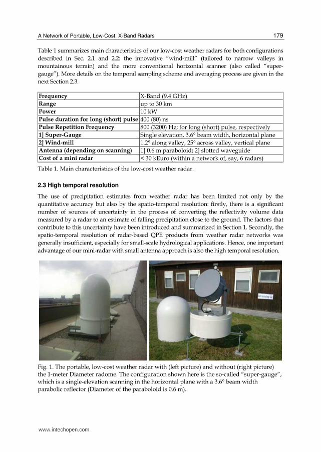
Cost, radiation safety issues and aesthetic issues motivate the use of small antennas and low-power transmitters that could be installed on either low-cost towers or existing infrastructures such as rooftops of existing buildings or telecommunication poles. This requires that the radars are physically small and that the radiated power levels are low enough so as not to pose an actual or perceived radiation safety hazard. We have opted for a very small parabolic antenna (D = 0.6 m) which corresponds to a 3 dB cross-range spatial resolution of 1 km at 20 km range (two third of the used range, which is 30 km). The antenna is hidden below a 1 m diameter radome (Fig. 1, left picture) and rotates at ~120° per second using a single elevation.

One precipitation map is made available every minute by averaging 16 rotations (out of the 22 available) 9 consecutive rays and 2 range-bins, hence resulting in a total of 144 samples.

www.intechopen.com


179

Table 1 summarizes main characteristics of our low-cost weather radars for both configurations

described in Sec. 2.1 and 2.2: the innovative “wind-mill” (tailored to narrow valleys in

mountainous terrain) and the more conventional horizontal scanner (also called “super-

gauge”). More details on the temporal sampling scheme and averaging process are given in the

next Section 2.3.

Frequency X-Band (9.4 GHz)

Range up to 30 km

Power 10 kW

Pulse duration for long (short) pulse 400 (80) ns

Pulse Repetition Frequency 800 (3200) Hz; for long (short) pulse, respectively

1] Super-Gauge Single elevation, 3.6° beam width, horizontal plane

2] Wind-mill 1.2° along valley, 25° across valley, vertical plane

Antenna (depending on scanning) 1] 0.6 m paraboloid; 2] slotted waveguide

Cost of a mini radar < 30 kEuro (within a network of, say, 6 radars)

Table 1. Main characteristics of the low-cost weather radar.

2.3 High temporal resolution

The use of precipitation estimates from weather radar has been limited not only by the

quantitative accuracy but also by the spatio-temporal resolution: firstly, there is a significant

number of sources of uncertainty in the process of converting the reflectivity volume data

measured by a radar to an estimate of falling precipitation close to the ground. The factors that

contribute to this uncertainty have been introduced and summarized in Section 1. Secondly, the

spatio-temporal resolution of radar-based QPE products from weather radar networks was

generally insufficient, especially for small-scale hydrological applications. Hence, one important

advantage of our mini-radar with small antenna approach is also the high temporal resolution.

Fig. 1. The portable, low-cost weather radar with (left picture) and without (right picture) the 1-meter Diameter radome. The configuration shown here is the so-called “super-gauge”, which is a single-elevation scanning in the horizontal plane with a 3.6° beam width parabolic reflector (Diameter of the paraboloid is 0.6 m).

www.intechopen.com


180

As described in Sec. 2.2, both kinds of mini radar, the “wind-mill” (vertical plane scanning

along valley) and the “super-gauge” (which implements the traditional horizontal scan)

currently deliver an image of precipitation every minute; furthermore, the temporal

resolution can easily be reduced to 30 or even 15 s.

We here describe in more details how the time-averaged (1-minute-sampled) radar

reflectivity measurements are acquired. For each of the 9 consecutive shots, 2 contiguous

pulses have been acquired: the 2 contiguous pulses are separated by the pulse width,

which is 400 ns; the 9 consecutive shots are separated by the pulse repetition interval,

which is 1.25 ms. Every minute, the antenna performs 22 revolutions; however only data

from the first 16 revolutions (out of 22) were averaged on a linear power scale (algebraic

average: dBm values are antilog transformed, then averaged, then again transformed on a

decibel logarithmic scale). This means a total of 288 (18 times 16) samples; among them, at

least 216 are independent, if we assume a decorrelation time of ~10 ms (Fig. 1.14,

Sauvageot [1992]): sample #1 and # 9 of the 9 consecutive rays are in fact separated by

9×1.25 = 11.25 ms.

3. A few qualitative examples

3.1 An hostile environment: Detecting precipitation even inside a narrow valley

At the beginning of November 2011 (from 3 to 9 November around noon) six days of

continuous, wide-spread precipitation hit the north-western part of Italy (see Fig. 2). In the

south-western Alps and in the surrounding flatlands and hills, in fact, autumn is the season

in which the longest and heaviest rainfalls occur. This fact has long been known: a

description of these “late-summer” Mediterranean storms can already be found in the works

by the old-Roman author, Plinius. It can been explained in simple terms as follows: in

autumn the Mediterranean Sea surface temperature is still high, while cold air is already

forming over the central-northern part of Europe. This has two effects: first of all, the

thermal contrast facilitates the deepening of pressure low over the north-western part of the

Mediterranean Sea; secondly, the warm air that arrives from the south, flowing over the

Mediterranean, provides a ready source of moisture.

The enforced rising of this warm-humid convectively unstable air, thanks to the Alpine

barrier, causes extensive and heavy rainfall. One has the impression of being subject to a

long storm, but, in reality, it is the continuous formation of stormy cells over the same

place.

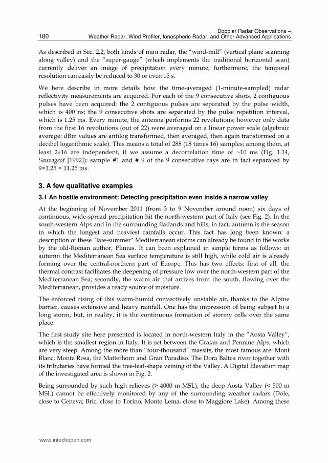
The first study site here presented is located in north-western Italy in the “Aosta Valley”,

which is the smallest region in Italy. It is set between the Graian and Pennine Alps, which

are very steep. Among the more than “four-thousand” massifs, the most famous are: Mont

Blanc, Monte Rosa, the Matterhorn and Gran Paradiso. The Dora Baltea river together with

its tributaries have formed the tree-leaf-shape veining of the Valley. A Digital Elevation map

of the investigated area is shown in Fig. 2.

Being surrounded by such high relieves (> 4000 m MSL), the deep Aosta Valley (< 500 m

MSL) cannot be effectively monitored by any of the surrounding weather radars (Dole,

close to Geneva; Bric, close to Torino; Monte Lema, close to Maggiore Lake). Among these

www.intechopen.com


181

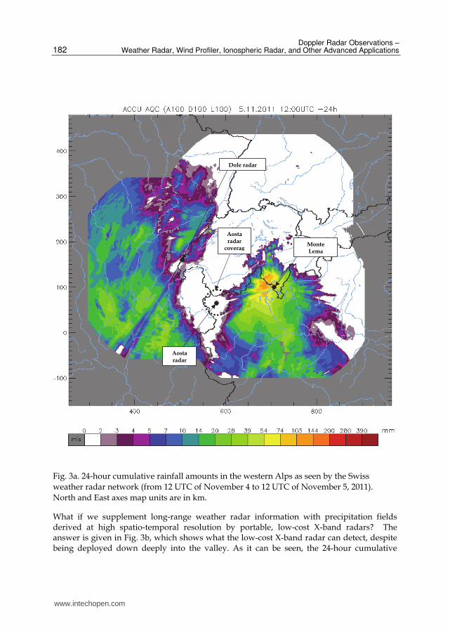
three radars, the one with “less worse” visibility is certainly Monte Lema, which was the

only one able to detect some weak echoes during the 24-hour period shown in Fig. 3a (from

12 UTC of November 4 to 12 UTC of November 5). However, because of beam shielding by

relieves combined with overshooting, the 24-hour radar-derived rainfall amounts above the

central-western part of the Aosta Valley are heavily underestimated: for instance, above

Aosta town, the Swiss weather radar network (see Fig. 3a) shows amounts smaller than 2

mm in 24 hours.

Fig. 2. Digital Elevation map of the north-western part of Italy.

www.intechopen.com


182

Fig. 3a. 24-hour cumulative rainfall amounts in the western Alps as seen by the Swiss

weather radar network (from 12 UTC of November 4 to 12 UTC of November 5, 2011).

North and East axes map units are in km.

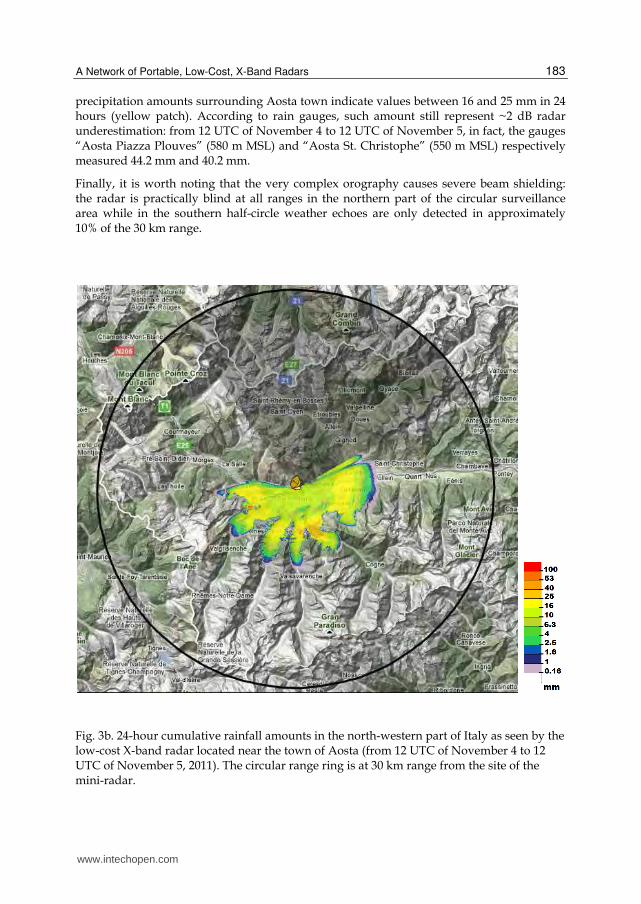
What if we supplement long-range weather radar information with precipitation fields derived at high spatio-temporal resolution by portable, low-cost X-band radars? The answer is given in Fig. 3b, which shows what the low-cost X-band radar can detect, despite being deployed down deeply into the valley. As it can be seen, the 24-hour cumulative

www.intechopen.com


183

precipitation amounts surrounding Aosta town indicate values between 16 and 25 mm in 24 hours (yellow patch). According to rain gauges, such amount still represent ~2 dB radar underestimation: from 12 UTC of November 4 to 12 UTC of November 5, in fact, the gauges “Aosta Piazza Plouves” (580 m MSL) and “Aosta St. Christophe” (550 m MSL) respectively measured 44.2 mm and 40.2 mm.

Finally, it is worth noting that the very complex orography causes severe beam shielding: the radar is practically blind at all ranges in the northern part of the circular surveillance area while in the southern half-circle weather echoes are only detected in approximately 10% of the 30 km range.

Fig. 3b. 24-hour cumulative rainfall amounts in the north-western part of Italy as seen by the low-cost X-band radar located near the town of Aosta (from 12 UTC of November 4 to 12 UTC of November 5, 2011). The circular range ring is at 30 km range from the site of the mini-radar.

www.intechopen.com


184

3.2 The extreme spatio-temporal variability of the precipitation field in semi-arid regions

In this section, a typical Mediterranean thunderstorm hitting the Palermo town in Sicily is

presented. More details are given in the caption of Fig. 4 below, while QPE performances of

the Palermo mini radar are thoroughly discussed in Sec. 4.2.1 and 4.2.2.

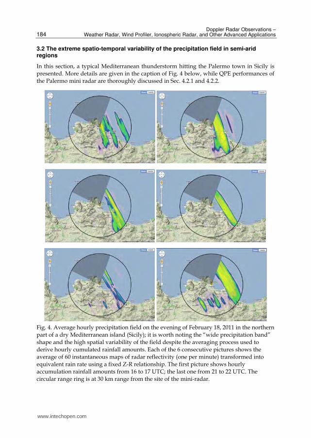
Fig. 4. Average hourly precipitation field on the evening of February 18, 2011 in the northern

part of a dry Mediterranean island (Sicily); it is worth noting the “wide precipitation band”

shape and the high spatial variability of the field despite the averaging process used to

derive hourly cumulated rainfall amounts. Each of the 6 consecutive pictures shows the

average of 60 instantaneous maps of radar reflectivity (one per minute) transformed into

equivalent rain rate using a fixed Z-R relationship. The first picture shows hourly

accumulation rainfall amounts from 16 to 17 UTC; the last one from 21 to 22 UTC. The

circular range ring is at 30 km range from the site of the mini-radar.

www.intechopen.com


185

4. Some quantitative examples in Sicily and Piedmont

4.1 Quantitative precipitation estimation (QPE)

While Section 3 dealt with qualitative examples, in the present Section 4 we will present hourly radar-derived precipitation amounts as obtained from weather echoes aloft to be compared with point rainfall measurements acquired at the ground by rain gauges.

4.1.1 From instantaneous radar reflectivity to hourly rain rate amounts

We have seen in Sec. 2.3 that the mini-radar finally provides an instantaneous radar reflectivity value once per minute for each radar bin of 3° by 120 m. This value is in turn the average of 288 samples (among them, at least 32 samples are independent, see Sec. 2.3).

It is well known that the backscattered power caused by rain drops is, unfortunately, only indirectly linked to the rain rate, R ([R] = mm/h). The backscattered power caused by the hydrometeors and detected by the radar is, in fact, directly proportional to the radar reflectivity factor, Z. A fundamental quantity for precise assessment of both Z and R is the drop size distribution (DSD), N(D), which is defined as the number of rain drops per unit

volume in the diameter interval D, i.e. between the diameter D and D+D. The radar reflectivity factor, Z, is defined as the 6th moment of the DSD, namely:

6

0( )Z N D D dD

. (1)

In radar meteorology, it is common to use the dimensions of mm for drop diameter, D, and to consider the summation (integral) to take place over a unit volume of 1 m3. Therefore, the conventional unit of Z is in mm6/m3. For the assessment of rain rate, another fundamental

quantity is needed: the terminal drops fall velocity as a function of the diameter, (D). Since

it is common to use [] = m/s, then the relationship is

4 3

06 10 ( ) ( )R D D v D dD . (2)

If precipitating hydrometeors in the radar backscattering volume were all spherical raindrops (which is almost never the case!) and the DSD could be described to a good approximation by an exponential DSD, then a simple power-law would relate Z to R. The first ever exponential DSD presented in a peer-reviewed paper and probably the most quoted is the Marshall-Palmer (M-P) distribution. The power law derived using the exponential fit proposed in Eq. (1)

and (3) of the famous paper by Marshall and Palmer [1948] is Z=296R1.47.

Here we have used the following Z-R relationship Z = 316R1.5 to derive the variable of interest, R, from the geophysical observable, Z, which is detected by the meteorological radar. Such values have been retrieved by Doelling et al. [1998] using seven years of measurements in central Europe. It is also worth noting that for the 2 radars in Sicily prior to any processing, the radar reflectivity values were increased by 4 dB to compensate system losses not properly compensated in the ‘‘traditional’’ radar equation.

For each radar bin, a maximum of 60 clutter-free radar reflectivity values are then

transformed into R using 2/3( / 316)R Z and then averaged to derive the corresponding

hourly rain rate used in this study.

www.intechopen.com


186

4.1.2 QPE evaluation based on the comparison between hourly radar and gauge rainfall amounts

The evaluation is based by looking at the average value and the dispersion of the errors (we call error the disagreement between radar and gauge amounts). For such characterization,

we define the two following parameters:

1. Bias (in dB). The bias in dB is defined as the ratio between radar and gauge total

precipitation amounts on a logarithmic (decibel) scale. It describes the overall agreement between radar estimates and ground point measurements. It is averaged

over the whole space–time window of the sample. A positive (negative) bias in dB denotes an overall radar overestimation (underestimation).

2. Scatter (in dB). The definition of scatter is strictly connected to the selected error distribution from a hydrological (end-user) and radar-meteorological (operational

remotely sensed samples of the spatio-temporal variability of the precipitation field) perspective. The error distribution is expressed as the cumulative contribution to

total rainfall (hydrologist point of view, y axis) as a function of the radar–gauge ratio (radar-meteorologist point of view, x axis). Most of the sources of error in radar

precipitation estimates, in fact, have a multiplicative (rather than an additive) nature. An example of the error distribution is shown in Fig. 2 and 3 of Germann et

al. [2004]. The scatter is defined as half the distance between the 16% and 84% percentiles of the error distribution. The scatter refers to the spread of radar–gauge

ratios when pooling together all volumetric radar estimates aloft and point measurements at the ground.

From our radar-meteorological point of view the multiplicative nature of the error prevails with respect to the additive one. For example, water on the radome, a wrong calibration

radar constant, or a bad estimate of the profile all result in a multiplicative error (i.e. a factor) rather than an additive error (i.e. a difference). This is why bias, error distribution

and scatter are expressed as ratios in dB. A 3 dB scatter, for instance, means that radar–gauge ratios vary by a factor of 2. If bias is zero, it is interpreted as follows: the radar-

derived estimate lies within a factor of 2 of the gauge estimate for 68% of rainfall while for the remaining 32% the uncertainty is larger. The scatter as defined above is a robust measure

of the spread. It is insensitive to outliers for two reasons. First, each radar–gauge pair is weighted by its contribution to total rainfall (y axis of the cumulative error distribution). An

ill-defined large ratio that results from two small values, e.g. 0.4 mm/2 mm ~ −7 dB, describes an irrelevant event from a hydrological point of view, and only gets little weight.

Second, by taking the distance between the 16% and the 84% percentiles, the tails of the error distribution are not overrated. Another important advantage of the spread measure is

that it is unaffected by the bias error, hence providing a complementary view of the error in the estimates. The above definition of the scatter is thus a better measure of the spread than

the less resilient standard deviation.

4.2 Quantitative precipitation estimation for the Palermo radar

The Palermo radar is located on a small hill next to the harbor of the capital of Sicily (blue triangle, Fig. 5): its latitude is 38°.1139; its longitude is 13°.358; its altitude is 45 m above Mean Sea Level (MSL). The radar has been installed in autumn 2010.

www.intechopen.com


187

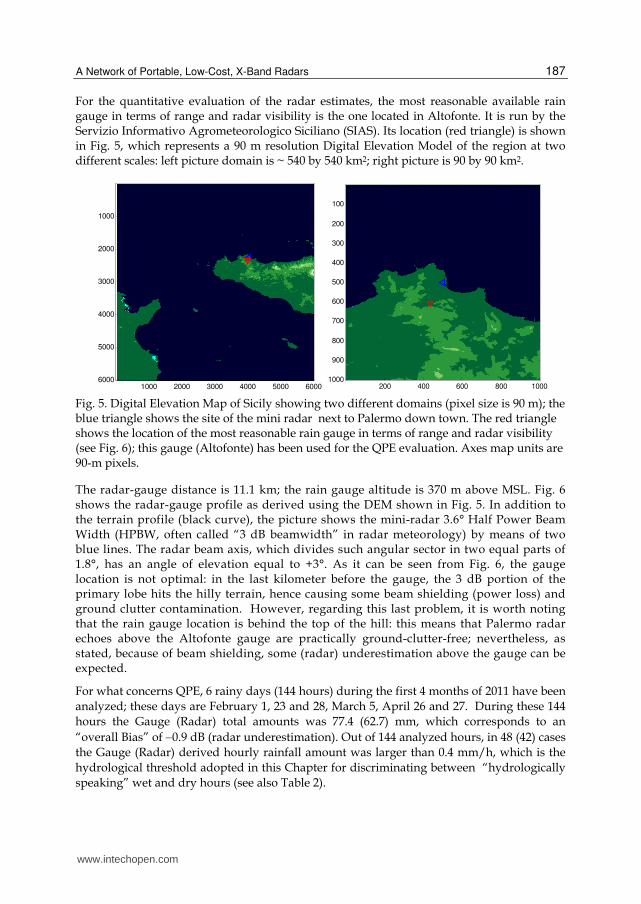
For the quantitative evaluation of the radar estimates, the most reasonable available rain gauge in terms of range and radar visibility is the one located in Altofonte. It is run by the Servizio Informativo Agrometeorologico Siciliano (SIAS). Its location (red triangle) is shown in Fig. 5, which represents a 90 m resolution Digital Elevation Model of the region at two different scales: left picture domain is ~ 540 by 540 km2; right picture is 90 by 90 km2.

1000 2000 3000 4000 5000 6000

1000

2000

3000

4000

5000

6000 200 400 600 800 1000

100

200

300

400

500

600

700

800

900

1000

Fig. 5. Digital Elevation Map of Sicily showing two different domains (pixel size is 90 m); the blue triangle shows the site of the mini radar next to Palermo down town. The red triangle shows the location of the most reasonable rain gauge in terms of range and radar visibility (see Fig. 6); this gauge (Altofonte) has been used for the QPE evaluation. Axes map units are 90-m pixels.

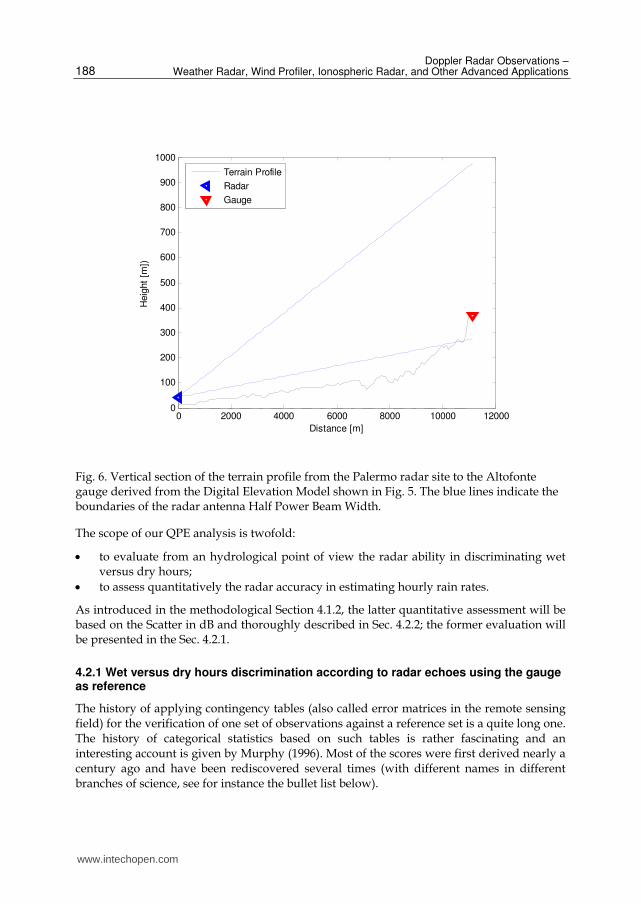
The radar-gauge distance is 11.1 km; the rain gauge altitude is 370 m above MSL. Fig. 6 shows the radar-gauge profile as derived using the DEM shown in Fig. 5. In addition to the terrain profile (black curve), the picture shows the mini-radar 3.6° Half Power Beam Width (HPBW, often called “3 dB beamwidth” in radar meteorology) by means of two blue lines. The radar beam axis, which divides such angular sector in two equal parts of 1.8°, has an angle of elevation equal to +3°. As it can be seen from Fig. 6, the gauge location is not optimal: in the last kilometer before the gauge, the 3 dB portion of the primary lobe hits the hilly terrain, hence causing some beam shielding (power loss) and ground clutter contamination. However, regarding this last problem, it is worth noting that the rain gauge location is behind the top of the hill: this means that Palermo radar echoes above the Altofonte gauge are practically ground-clutter-free; nevertheless, as stated, because of beam shielding, some (radar) underestimation above the gauge can be expected.

For what concerns QPE, 6 rainy days (144 hours) during the first 4 months of 2011 have been

analyzed; these days are February 1, 23 and 28, March 5, April 26 and 27. During these 144

hours the Gauge (Radar) total amounts was 77.4 (62.7) mm, which corresponds to an

“overall Bias” of 0.9 dB (radar underestimation). Out of 144 analyzed hours, in 48 (42) cases

the Gauge (Radar) derived hourly rainfall amount was larger than 0.4 mm/h, which is the

hydrological threshold adopted in this Chapter for discriminating between “hydrologically

speaking” wet and dry hours (see also Table 2).

www.intechopen.com


188

0 2000 4000 6000 8000 10000 120000

100

200

300

400

500

600

700

800

900

1000

Distance [m]

Heig

ht

[m])

Terrain Profile

Radar

Gauge

Fig. 6. Vertical section of the terrain profile from the Palermo radar site to the Altofonte gauge derived from the Digital Elevation Model shown in Fig. 5. The blue lines indicate the boundaries of the radar antenna Half Power Beam Width.

The scope of our QPE analysis is twofold:

to evaluate from an hydrological point of view the radar ability in discriminating wet versus dry hours;

to assess quantitatively the radar accuracy in estimating hourly rain rates.

As introduced in the methodological Section 4.1.2, the latter quantitative assessment will be based on the Scatter in dB and thoroughly described in Sec. 4.2.2; the former evaluation will be presented in the Sec. 4.2.1.

4.2.1 Wet versus dry hours discrimination according to radar echoes using the gauge as reference

The history of applying contingency tables (also called error matrices in the remote sensing field) for the verification of one set of observations against a reference set is a quite long one. The history of categorical statistics based on such tables is rather fascinating and an interesting account is given by Murphy (1996). Most of the scores were first derived nearly a century ago and have been rediscovered several times (with different names in different branches of science, see for instance the bullet list below).

www.intechopen.com


189

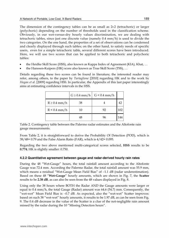
The dimension of the contingency tables can be as small as 22 (tetrachoric) or larger (polychoric) depending on the number of thresholds used in the classification scheme. Obviously, in our wet-versus-dry hourly values discrimination, we are dealing with tetrachoric tables, since just one discrete value (namely 0.4 mm/h) is used to divide the two categories. On the one hand, the properties of a set of observations can be condensed and clearly displayed through such tables; on the other hand, to satisfy needs of specific users, even for a simple tetrachoric table, several different scores have been introduced. Here, we will use two scores that can be applied to both tetrachoric and polychoric tables:

the Heidke Skill Score (HSS), also known as Kappa Index of Agreement (KIA), Khat, …

the Hanssen-Kuipers (HK) score also known as True Skill Score (TSS), …

Details regarding these two scores can be found in literature; the interested reader may refer, among others, to the paper by Tartaglione [2010] regarding HK and to the work by Hogan et al. [2009] regarding HSS. In particular, the Appendix of this last paper interestingly aims at estimating confidence intervals in the HSS.

G 0.4 mm/h G < 0.4 mm/h

R 0.4 mm/h 38 4 42

R < 0.4 mm/h 10 92 102

48 96 144

Table 2. Contingency table between the Palermo radar estimates and the Altofonte rain gauge measurements.

From Table 2, it is straightforward to derive the Probability Of Detection (POD), which is 38/48= 0.79 and the False Alarm Ratio (FAR), which is 4/42= 0.095.

Regarding the two above mentioned multi-categorical scores selected, HSS results to be 0.774; HK is slightly smaller: 0.750.

4.2.2 Quantitative agreement between gauge and radar-derived hourly rain rates

During the 48 “Wet-Gauge” hours, the total rainfall amount according to the Altofonte Gauge was 72.4 mm. According the Palermo Radar, the total rainfall amount was 55.9 mm,

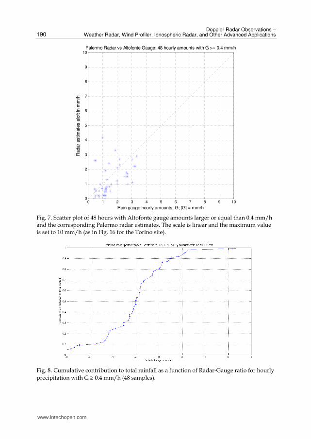
which means a residual “Wet-Gauge Mean Field Bias” of 1.1 dB (radar underestimation). Based on these 48 “Wet-Gauge” hourly amounts, which are shown in Fig. 7, the Scatter results to be 2.38 dB, as can also be seen from the 48 values displayed in Fig. 8.

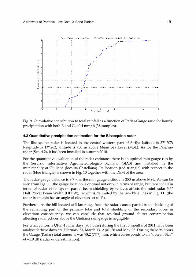
Using only the 38 hours where BOTH the Radar AND the Gauge amounts were larger or equal to 0.4 mm/h, the total Gauge (Radar) amount was 64.6 (54.7) mm. Consequently, the

“wet-wet” Mean Field Bias is 0.7 dB. As expected, also the “wet-wet” Scatter improves: based on such 38 “wet-wet” hourly amounts, it results to be 1.97 dB, as can be seen from Fig. 9. The 0.4 dB decrease in the value of the Scatter is a clue of the not-negligible rain amount missed by the radar during the 10 “Missing Detection hours”.

www.intechopen.com


190

0 1 2 3 4 5 6 7 8 9 100

1

2

3

4

5

6

7

8

9

10

Rain gauge hourly amounts, G; [G] = mm/h

Radar

estim

ate

s a

loft in

mm

/h

Palermo Radar vs Altofonte Gauge: 48 hourly amounts with G >= 0.4 mm/h

Fig. 7. Scatter plot of 48 hours with Altofonte gauge amounts larger or equal than 0.4 mm/h and the corresponding Palermo radar estimates. The scale is linear and the maximum value is set to 10 mm/h (as in Fig. 16 for the Torino site).

Fig. 8. Cumulative contribution to total rainfall as a function of Radar-Gauge ratio for hourly

precipitation with G 0.4 mm/h (48 samples).

www.intechopen.com


191

Fig. 9. Cumulative contribution to total rainfall as a function of Radar-Gauge ratio for hourly

precipitation with both R and G 0.4 mm/h (38 samples).

4.3 Quantitative precipitation estimation for the Bisacquino radar

The Bisacquino radar is located in the central-western part of Sicily: latitude is 37°.707; longitude is 13°.262; altitude is 780 m above Mean Sea Level (MSL). As for the Palermo radar (Sec. 4.2), it has been installed in autumn 2010.

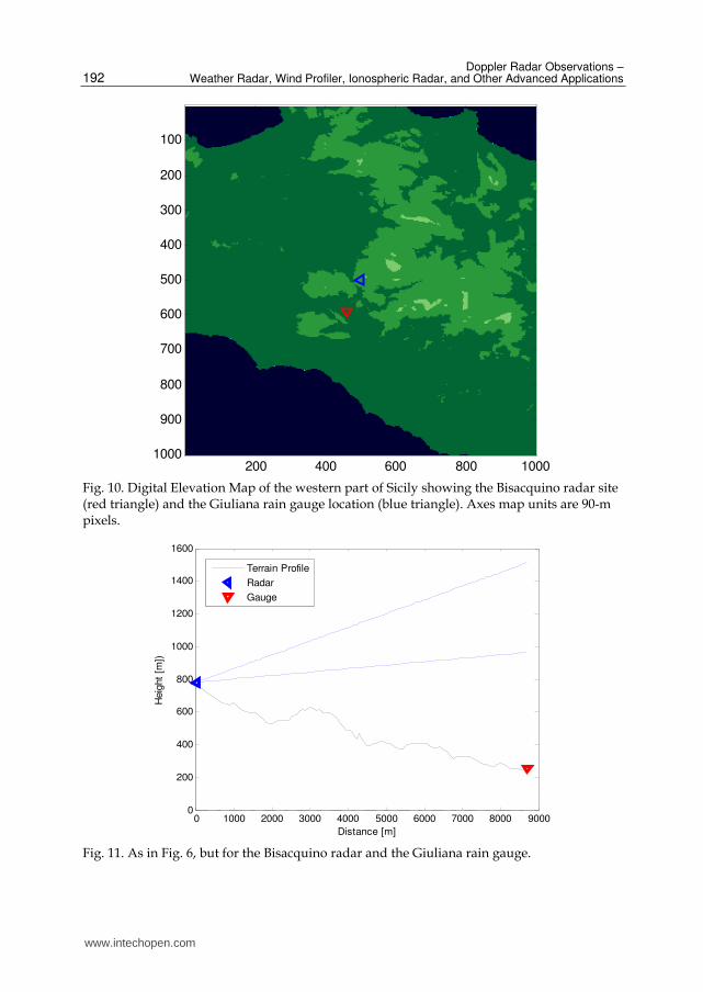
For the quantitative evaluation of the radar estimates there is an optimal rain gauge run by the Servizio Informativo Agrometeorologico Siciliano (SIAS) and installed in the municipality of Giuliana (località Castellana). Its location (red triangle) with respect to the radar (blue triangle) is shown in Fig. 10 together with the DEM of the area.

The radar-gauge distance is 8.7 km; the rain gauge altitude is 250 m above MSL. As can be seen from Fig. 11, the gauge location is optimal not only in terms of range, but most of all in terms of radar visibility: no partial beam shielding by relieves affects the mini radar 3.6° Half Power Beam Width (HPBW), which is delimited by the two blue lines in Fig. 11 (the radar beam axis has an angle of elevation set to 1°).

Furthermore, the hill located at 3 km range from the radar, causes partial beam shielding of the remaining part of the primary lobe and total shielding of the secondary lobes in elevation; consequently, we can conclude that residual ground clutter contamination affecting radar echoes above the Giuliana rain gauge is negligible.

For what concerns QPE, 4 rainy days (96 hours) during the first 5 months of 2011 have been analyzed; these days are February 23, March 13, April 26 and May 22. During these 96 hours the Gauge (Radar) total amounts was 98.2 (77.7) mm, which corresponds to an “overall Bias”

of 1.0 dB (radar underestimation).

www.intechopen.com


192

200 400 600 800 1000

100

200

300

400

500

600

700

800

900

1000

Fig. 10. Digital Elevation Map of the western part of Sicily showing the Bisacquino radar site (red triangle) and the Giuliana rain gauge location (blue triangle). Axes map units are 90-m pixels.

0 1000 2000 3000 4000 5000 6000 7000 8000 90000

200

400

600

800

1000

1200

1400

1600

Distance [m]

Heig

ht

[m])

Terrain Profile

Radar

Gauge

Fig. 11. As in Fig. 6, but for the Bisacquino radar and the Giuliana rain gauge.

www.intechopen.com


193

Out of 96 analyzed hours, in 37 (34) cases the Gauge (Radar) derived hourly rainfall amount was larger than 0.4 mm/h (see the next Sec. 4.3.1 and Table 3 for more details).

4.3.1 Wet versus dry hours discrimination

From Table 3, it is easy to see that in this case the POD is (29/37) 0.78 while the FAR is relatively high: (5/34) 0.15. If we consider scores that deal with all the elements of the table, then HSS results to be 0.710 while HK is quite similar: 0.699.

G 0.4 mm/h

G < 0.4 mm/h

R 0.4 mm/h 29 5 34

R < 0.4 mm/h 8 54 62

37 59 96

Table 3. Contingency table between the Bisacquino radar observations and the Giuliana rain gauge measurements during the 96-hour observation period.


During the 37 “Wet-Gauge hours”, the total rainfall amount according to the Giuliana Gauge was 97.4 mm. According to the Palermo Radar, the total rainfall amount was 74.6

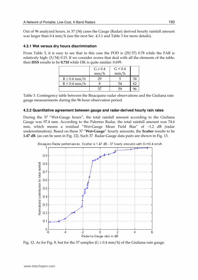
mm, which means a residual “Wet-Gauge Mean Field Bias” of 1.2 dB (radar underestimation). Based on these 37 “Wet-Gauge” hourly amounts, the Scatter results to be 1.47 dB. (as can be seen in Fig. 12). Such 37 Radar-Gauge data pairs are shown in Fig. 13.

Fig. 12. As for Fig. 8, but for the 37 samples (G 0.4 mm/h) of the Giuliana rain gauge.

www.intechopen.com


194

0 2 4 6 8 10 12 14 16 18 200

2

4

6

8

10

12

14

16

18

20


Radar

estim

ate

s a

loft in

mm

/h

Bisaquino Radar vs Giuliana Gauge: 37 hourly amounts with G >= 0.4 mm/h

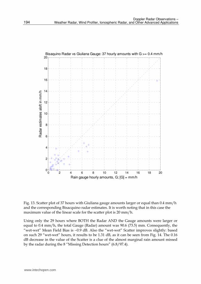
Fig. 13. Scatter plot of 37 hours with Giuliana gauge amounts larger or equal than 0.4 mm/h and the corresponding Bisacquino radar estimates. It is worth noting that in this case the maximum value of the linear scale for the scatter plot is 20 mm/h.

Using only the 29 hours where BOTH the Radar AND the Gauge amounts were larger or equal to 0.4 mm/h, the total Gauge (Radar) amount was 90.6 (73.5) mm. Consequently, the

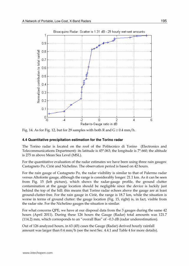
“wet-wet” Mean Field Bias is 0.9 dB. Also the “wet-wet” Scatter improves slightly: based on such 29 “wet-wet” hours, it results to be 1.31 dB, as it can be seen from Fig. 14. The 0.16 dB decrease in the value of the Scatter is a clue of the almost marginal rain amount missed by the radar during the 8 “Missing Detection hours” (6.8/97.4).

www.intechopen.com


195

Fig. 14. As for Fig. 12, but for 29 samples with both R and G 0.4 mm/h.

4.4 Quantitative precipitation estimation for the Torino radar

The Torino radar is located on the roof of the Politecnico di Torino (Electronics and Telecommunications Department): its latitude is 45°.063; the longitude is 7°.660; the altitude is 275 m above Mean Sea Level (MSL).

For the quantitative evaluation of the radar estimates we have been using three rain gauges: Castagneto Po, Ciriè and Nichelino. The observation period is based on 42 hours.

For the rain gauge of Castagneto Po, the radar visibility is similar to that of Palermo radar versus Altofonte gauge, although the range is considerably longer: 21.1 km. As it can be seen from Fig. 15 (left picture), which shows the radar-gauge profile, the ground clutter contamination at the gauge location should be negligible since the device is luckily just behind the top of the hill: this means that Torino radar echoes above the gauge are at least ground-clutter-free. For the rain gauge in Ciriè, the range is 18.7 km, while the situation is worse in terms of ground clutter: the gauge location (Fig. 15, right) is, in fact, visible from the radar site. For the Nichelino gauges the situation is similar.

For what concerns QPE, we have at our disposal data from the 3 gauges during the same 42 hours (April 2011). During these 126 hours the Gauge (Radar) total amounts was 121.7

(114.2) mm, which corresponds to an “overall Bias” of 0.3 dB (radar underestimation).

Out of 126 analyzed hours, in 63 (45) cases the Gauge (Radar) derived hourly rainfall amount was larger than 0.4 mm/h (see the next Sec. 4.4.1 and Table 4 for more details).

www.intechopen.com


196

4.4.1 Wet versus dry hours discrimination

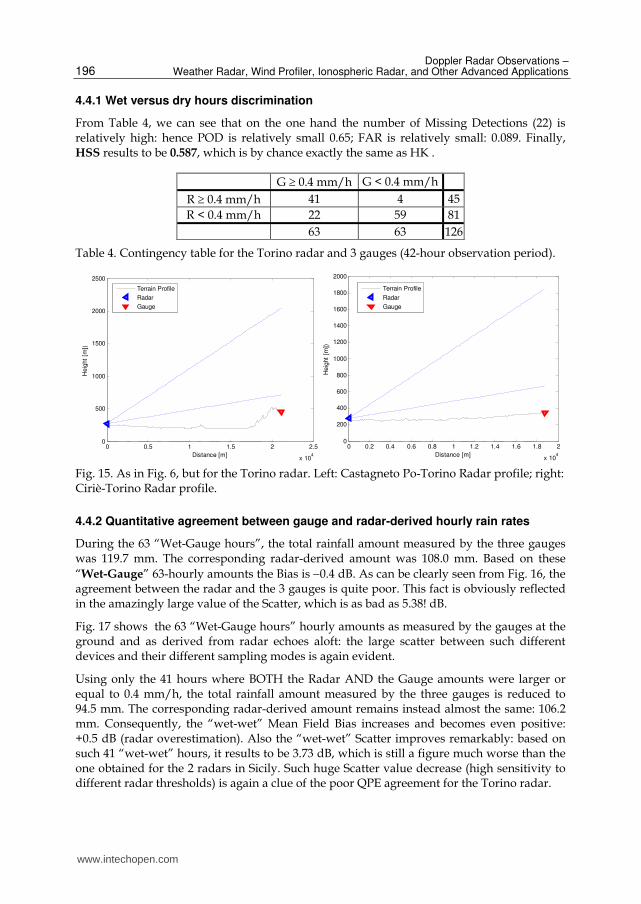
From Table 4, we can see that on the one hand the number of Missing Detections (22) is relatively high: hence POD is relatively small 0.65; FAR is relatively small: 0.089. Finally, HSS results to be 0.587, which is by chance exactly the same as HK .

G 0.4 mm/h G < 0.4 mm/h

R 0.4 mm/h 41 4 45

R < 0.4 mm/h 22 59 81

63 63 126

Table 4. Contingency table for the Torino radar and 3 gauges (42-hour observation period).

0 0.5 1 1.5 2 2.5

x 104

0

500

1000

1500

2000

2500

Distance [m]

Heig

ht

[m])

Terrain Profile

Radar

Gauge

0 0.2 0.4 0.6 0.8 1 1.2 1.4 1.6 1.8 2

x 104

0

200

400

600

800

1000

1200

1400

1600

1800

2000

Distance [m]

Heig

ht

[m])

Terrain Profile

Radar

Gauge

Fig. 15. As in Fig. 6, but for the Torino radar. Left: Castagneto Po-Torino Radar profile; right: Ciriè-Torino Radar profile.


During the 63 “Wet-Gauge hours”, the total rainfall amount measured by the three gauges was 119.7 mm. The corresponding radar-derived amount was 108.0 mm. Based on these

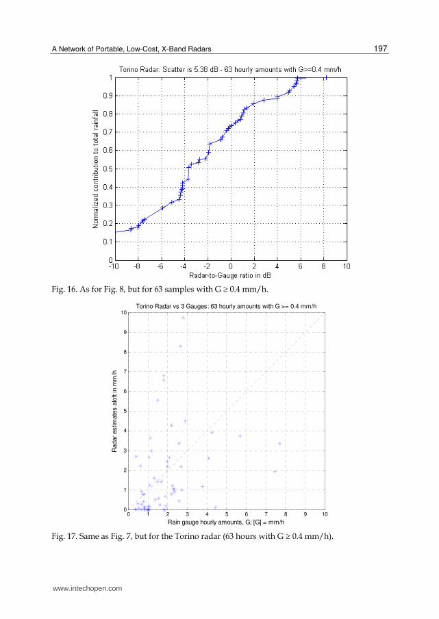
“Wet-Gauge” 63-hourly amounts the Bias is 0.4 dB. As can be clearly seen from Fig. 16, the agreement between the radar and the 3 gauges is quite poor. This fact is obviously reflected in the amazingly large value of the Scatter, which is as bad as 5.38! dB.

Fig. 17 shows the 63 “Wet-Gauge hours” hourly amounts as measured by the gauges at the ground and as derived from radar echoes aloft: the large scatter between such different devices and their different sampling modes is again evident.

Using only the 41 hours where BOTH the Radar AND the Gauge amounts were larger or equal to 0.4 mm/h, the total rainfall amount measured by the three gauges is reduced to 94.5 mm. The corresponding radar-derived amount remains instead almost the same: 106.2 mm. Consequently, the “wet-wet” Mean Field Bias increases and becomes even positive: +0.5 dB (radar overestimation). Also the “wet-wet” Scatter improves remarkably: based on such 41 “wet-wet” hours, it results to be 3.73 dB, which is still a figure much worse than the one obtained for the 2 radars in Sicily. Such huge Scatter value decrease (high sensitivity to different radar thresholds) is again a clue of the poor QPE agreement for the Torino radar.

www.intechopen.com


197

Fig. 16. As for Fig. 8, but for 63 samples with G 0.4 mm/h.

0 1 2 3 4 5 6 7 8 9 100

1

2

3

4

5

6

7

8

9

10


Radar

estim

ate

s a

loft in

mm

/h

Torino Radar vs 3 Gauges: 63 hourly amounts with G >= 0.4 mm/h

Fig. 17. Same as Fig. 7, but for the Torino radar (63 hours with G 0.4 mm/h).

www.intechopen.com


198

4.5 QPE Summary in terms of bias and scatter in dB

For the three mini-radar sites discussed in the previous paragraphs, Table 5 provides a summary of the QPE evaluation in terms of Bias in dB (as a function of the number of considered hours). When all the wet and dry hours are considered, we have the so-called “overall” Bias: it includes False Alarm events (mainly caused by ground clutter contamination) and Missing Detection (caused by beam overshooting, see Sec. 1.2 and, in some cases, attenuation) events; it is certainly the most resistant and complete definition of Bias. It is obviously a measure of the mean error and says nothing about the error dispersion around the mean. For this purpose, there is the Scatter, which will be presented in the Table 6.

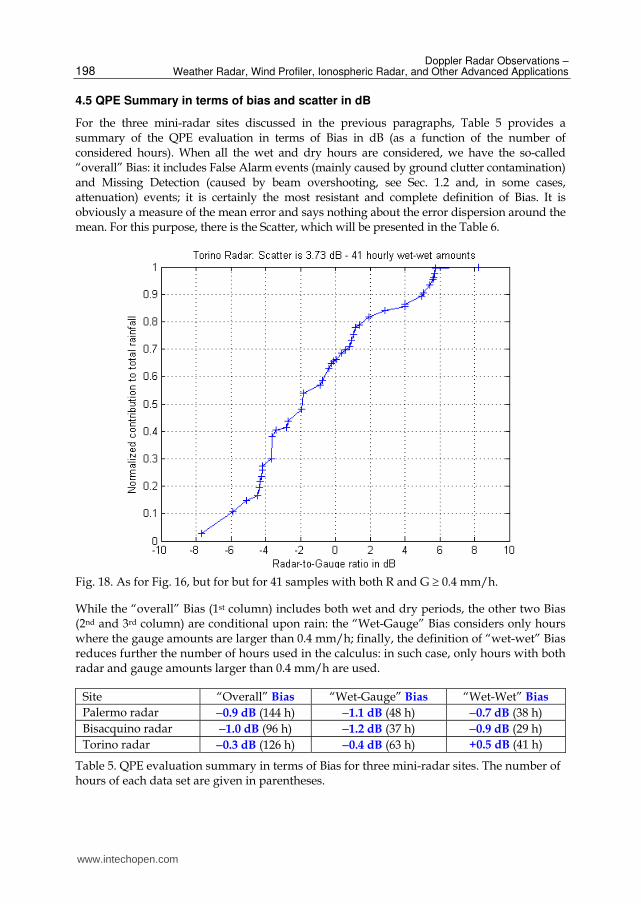
Fig. 18. As for Fig. 16, but for but for 41 samples with both R and G 0.4 mm/h.

While the “overall” Bias (1st column) includes both wet and dry periods, the other two Bias (2nd and 3rd column) are conditional upon rain: the “Wet-Gauge” Bias considers only hours where the gauge amounts are larger than 0.4 mm/h; finally, the definition of “wet-wet” Bias reduces further the number of hours used in the calculus: in such case, only hours with both radar and gauge amounts larger than 0.4 mm/h are used.

Site “Overall” Bias “Wet-Gauge” Bias “Wet-Wet” Bias

Palermo radar 0.9 dB (144 h) 1.1 dB (48 h) 0.7 dB (38 h)

Bisacquino radar 1.0 dB (96 h) 1.2 dB (37 h) 0.9 dB (29 h)

Torino radar 0.3 dB (126 h) 0.4 dB (63 h) +0.5 dB (41 h)

Table 5. QPE evaluation summary in terms of Bias for three mini-radar sites. The number of hours of each data set are given in parentheses.

www.intechopen.com


199

Table 6 summarizes the dispersion of the radar-gauge errors using the hydrological-oriented score called Scatter (see Sec. 4.1.2). Since, as discussed previously, in the radar detection process (see for instance the “multiplicative” nature of the meteorological radar equation derived by Probert-Jones [1962]), the multiplicative nature of error prevails, the Scatter is defined as a ratio between the Radar (the device under test) and the Gauge (the reference). Hence, dry hours cannot be considered in evaluating the Scatter (unless using some trick, like for instance adding a negligible amount…) Consequently, only “Wet-Gauge” hours or “wet-wet” hours are considered in Table 6.

It can be concluded that the three-presented X-band radars are less reliable at low rain rates. By limiting the observations to hours with both Radar and Gauge amounts larger than 0.4 mm/h, the agreement improves not only in terms of Bias, but most of all in terms of Scatter. Finally, in the interpretation of these values of Bias and Scatter, it is important to bear in mind the large intrinsically different sampling modes as well as mismatches in time of the radar and gauge devices (e.g. Zawadzki [1975]).

Site “Wet-Gauge” Scatter “Wet-Wet” Scatter

Palermo radar 2.38 dB (48 h) 1.97 dB (38 h)

Bisacquino radar 1.47 dB (37 h) 1.31 dB (29 h)

Torino radar 5.38 dB (63 h) 3.73 dB (41 h)

Table 6. QPE evaluation summary in terms of Scatter for three mini-radar sites. The number of hours of each data set are given in parentheses.

5. Open issues and limitations

Short-wavelength (X-band) radar has the benefit of attaining high spatial resolution with a

smaller antenna. However, there is a clear disadvantage compared to longer wavelengths: an

increased attenuation in the presence of precipitation. Imagine three 2-km convective cells with

instantaneous rain rate of 20, 40 and 100 mm/h respectively: at X-band frequencies these cells

would cause two-way attenuation in radar reflectivity values of approximately 1.5, 3.6! and 11!!

dB. Such figures preclude not only the use of X-band radar for long-range monitoring but also

an accurate QPE, even at short-range. A partial remedy could be the use of polarimetric

information, but this would remarkably increase the cost of the system: in the interesting work

by Mc Laughlin et. al [2009], the cost of a Doppler, fully Polarimetric advanced X-band system

developed within the framework of the CASA project is estimated in approximately 180 kEuro,

which is almost 8 dB more expensive than our low-cost, semi-quantitative approach.

6. Summary: Filling the gap, which is observing the lowest part of the troposphere at short-range with portable, low-cost radars

Radar sampling volume increases with the square of the range (beam broadening) therefore, at longer ranges, small but intense features of the precipitation system are blurred (non-homogeneous beam filling). Furthermore, it is more likely to include different types of hydrometeors (e.g. snow, ice, rain drops), especially in the vertical dimension. At long-range, because of the decreased vertical resolution, the lower part of the sampling volume can be in rain whereas the upper part can be even characterized by an echo weaker than the radar sensitivity itself (beam overshooting).

www.intechopen.com


200

By the term “range degradation” we mean several important sources of uncertainty

regarding radar-based estimates of rainfall: beam broadening, non-homogeneous beam

filling, partial beam occultation, overshooting and, depending on the operating frequency,

attenuation. Such sources of uncertainty in general increase with increasing range. Current

approaches to operational weather observation are based on the use of physically large,

high-power, long-range radars, which are blocked from viewing the lower part of the

troposphere by the Earth’s curvature combined with orography. Hence, range degradation

is one of the main problems in QPE and certainly a key factor in the underestimation of

rainfall accumulation at far ranges with conventional long-range radars (e.g. Kitchen and

Jackson [1993], Smith et al. [1996], Meischner et al. [1997], Seo et al. [2000], Gabella et al. [2000],

Chumechean et al. [2004], Joss et al. [2006]).

This Chapter describes an alternate approach based on networks of large number of small,

low-cost, X-band radars. Spacing these radars twenty kilometers apart defeats the Earth’s

curvature problem and enables the sampling of the lowest part of the troposphere using

small antennas and low-power transmitters. Such networks can provide observing

capabilities which supplement the operational state of the art radar network satisfying at the

same time the needs of multiple users. Improved capabilities associated with this

technology include low-altitude coverage and high temporal resolution. This technology has

the potential to supplement the widely spaced networks of physically large high-power

radars in use today.

Indeed, short-wavelength low-cost radar is able to fill a remarkable gap in observational

meteorology: small, low-cost, radars can be used to supplement conventional, long-range

radar networks in complex orography regions (e.g. the Alps and the Apennines), in highly

populated areas (improving urban hydrology in major towns), in sensitive regions (areas

prone to hydro-geological hazards) and along technological networks (e.g. highways, gas

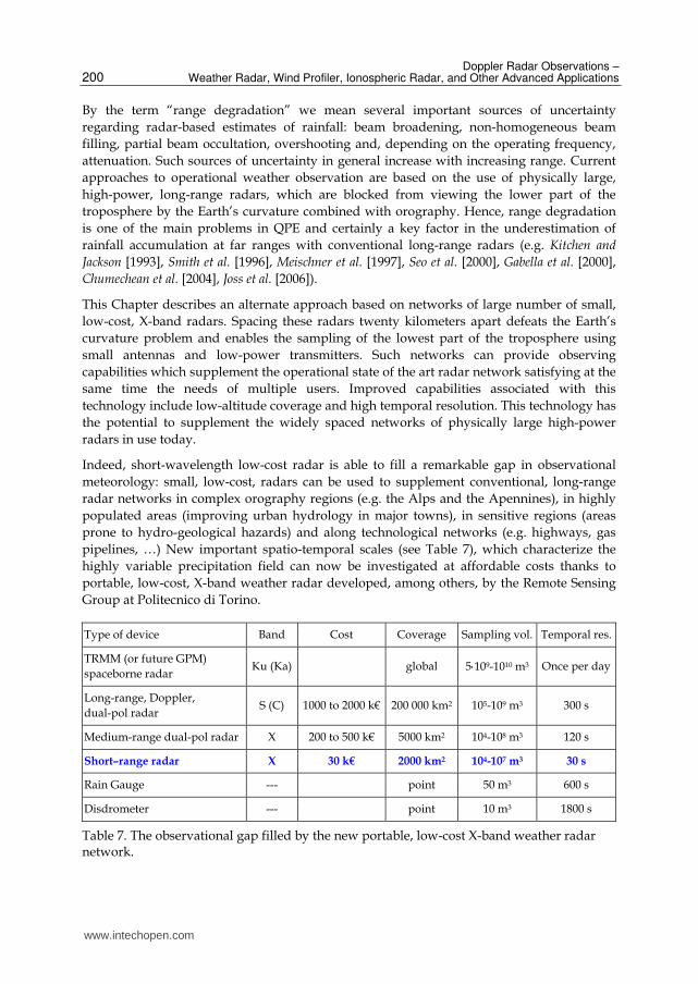
pipelines, …) New important spatio-temporal scales (see Table 7), which characterize the

highly variable precipitation field can now be investigated at affordable costs thanks to

portable, low-cost, X-band weather radar developed, among others, by the Remote Sensing

Group at Politecnico di Torino.

Type of device Band Cost Coverage Sampling vol. Temporal res.

TRMM (or future GPM)

spaceborne radar Ku (Ka) global 5109-1010 m3 Once per day

Long-range, Doppler,

dual-pol radar S (C) 1000 to 2000 k€ 200 000 km2 105-109 m3 300 s

Medium-range dual-pol radar X 200 to 500 k€ 5000 km2 104-108 m3 120 s

Short–range radar X 30 k€ 2000 km2 104-107 m3 30 s

Rain Gauge --- point 50 m3 600 s

Disdrometer --- point 10 m3 1800 s

Table 7. The observational gap filled by the new portable, low-cost X-band weather radar network.

www.intechopen.com


201

7. Acknowledgements

Gauge data were provided by the Regione Autonoma Valle d’Aosta – Ufficio Meteorologico della Protezione Civile, the Servizio Informativo Agrometeorologico Siciliano and Weather Underground. The mini radar development was possible thanks to the financial and technical support by Consorzio Interuniversitario per le Fisiche della Atmosfera (CINFAI).

8. References

Chumchean, S., Seed, A., and A. Sharma, 2004: Application of scaling in radar reflectivity for correcting range dependent bias in climatological radar rainfall estimates, J. Atmos. Ocean. Technol., 21, 1545-1556.

Doelling, I. G., J. Joss, and J. Riedl, Systematic variations of Z-R relationships from drop size distributions measured in Northern Germany during seven years, Atmos. Res., 48, 635-649, 1998.

Gabella, M., M. Bolliger, U. Germann, and G. Perona, 2005: Large sample evaluation of cumulative rainfall amounts in the Alps using a network of three radars, Atmos. Res., 77, 256-268.

Gabella, M., J. Joss, and G. Perona, 2000: Optimizing quantitative precipitation estimates using a non-coherent and a coherent radar operating on the same area, J. Geophys. Res., 105, 2237-2245.

Gabella M., Joss J., Michaelides S., Perona G., 2006: Range adjustment for Ground-based Radar, derived with the spaceborne TRMM Precipitation Radar, IEEE Trans. on Geosci. Rem. Sens., 44, 126-133, doi: 10.1109/ TGRS.2005.858436

Gabella M., Orione F., Zambotto M., Turso S., 2008: A Portable Low-Cost X-Band Radar For Rainfall Estimation In Alpine Valleys – Analysis of radar reflectivities and comparison between remotely sensed and in situ measurements, FORALPS Final Meeting Report, ISBN 978-88-8443-235-3, pp. 39.

Gabella M., Morin E., Notarpietro R., 2011a: Using TRMM spaceborne radar as a reference for compensating ground-based radar range degradation: Methodology verification based on rain gauges in Israel, J. Geophys. Res., 116, D02114, doi: 10.1029/2010JD014496

Gabella M., Morin E., Notarpietro R., Michaelides S., 2011b: Precipitation field in the Southeastern Mediterranean area as seen by the Ku-band spaceborne weather radar and two C-band ground-based radars, Atmos. Res., doi: 10.1016/j.atmosres2011.06.001.

Germann U., Galli G., Boscacci M., Bolliger M., Gabella M., 2004: Quantitative precipitation estimation in the Alps: where do we stand?, Third European Conference on Radar meteorology ERAD2004, Visby, Sweden, 2-6.

Hogan, R. J., O’Connor E. J. and A. J. Illingworth 2009: Verification of cloud-fraction forecasts, Q. J. Royal Meteorol. Soc., 135, 1494-1511.

Joss J., Gabella M., Michaelides S., and G. Perona, 2006: Variation of weather radar sensitivity at ground level and from space: case studies and possible causes, Meteorol. Z., 15, 485-496, doi: 10.1127/0941-2948/2006/0150.

Kitchen, M., and P.M. Jackson, 1993: Weather radar performance at long range simulated and observed, J. Appl. Meteor., 32, 975-985.

www.intechopen.com


202

Marshall, J. S. and W. M. Palmer, 1948: The distribution of raindrops with size, J. Meteor., 5, 165-166.

Mc Laughin and other 28 coauthors, 2009: Short-wavelength technology and the potential for distributed networks of small radar systems, Bull. Am. Meteorol. Soc., 90, 1797-1817.

Meischner, P., Collier, C., Illingworth, A., Joss J., and W. Randeu, 1997: Advanced weather radar systems in Europe: the COST 75 action, Bull. Am. Meteorol. Soc., 78, 1411–1430.

Murphy, A. H., 1996: The Finley affair: A signal event in the history of forecast verification,Weather Forecast., 11, 3–20.

Notarpietro R., Zambotto M., Gabella M., Turso S., Perona G., 2005: The radar-ombrometer: a portable, low-cost, short-range X-band radar for rain estimation within valleys, VOLTAIRE final conference joint with the 7th European Conference on Applications of Meteorology (ECAM7) and the European Meteorological Society meeting (EMS05), September 12-16, Utrecht, The Netherlands, 19.

Probert-Jones, J. R., 1962: The radar equation in meteorology, Quart. J. Royal Meteorol. Soc., 88, 485-495.

Seo, D. J., Breidenbach J., Fulton R., Miller D., and T. O’Bannon, 2000: Real-time adjustment of range-dependent biases in WSR-88D rainfall estimates due to non-uniform vertical profile of reflectivity. J. Hydrometeorol, 1, 222–240.

Smith, J. A., Seo D. J., Baeck M. L., Hudlow M. D., 1996: An inter-comparison study of NEXRAD precipitation estimates, Water Resour. Res., 32, 2035-2045.

Tartaglione N., 2010: Relationship between precipitation forecast errors and skill scores of dichotomous forecasts, Weath. Forec., 25, 355-364.

Young C. B., Nelson B. R., Bradley A. A., Smith J.A., Peters-Lidard C. D., Kruger A., Baeck M. L., 1999: An evaluation of NEXRAD precipitation estimates in complex terrain, J. Geophys. Res. Atmos., 104, 19691-19703.

Sauvageot, H., 1992: Radar Meteorology, Boston, Artech House. Zawadzki I., 1975: On radar-raingage comparison, J. Appl. Meteorol., 14, 1430-1436.

www.intechopen.com

Doppler Radar Observations - Weather Radar, Wind Profiler,Ionospheric Radar, and Other Advanced ApplicationsEdited by Dr. Joan Bech

ISBN 978-953-51-0496-4Hard cover, 470 pagesPublisher InTechPublished online 05, April, 2012Published in print edition April, 2012

InTech EuropeUniversity Campus STeP Ri Slavka Krautzeka 83/A 51000 Rijeka, Croatia Phone: +385 (51) 770 447 Fax: +385 (51) 686 166www.intechopen.com

InTech ChinaUnit 405, Office Block, Hotel Equatorial Shanghai No.65, Yan An Road (West), Shanghai, 200040, China

Phone: +86-21-62489820 Fax: +86-21-62489821

Doppler radar systems have been instrumental to improve our understanding and monitoring capabilities ofphenomena taking place in the low, middle, and upper atmosphere. Weather radars, wind profilers, andincoherent and coherent scatter radars implementing Doppler techniques are now used routinely both inresearch and operational applications by scientists and practitioners. This book brings together a collection ofeighteen essays by international leading authors devoted to different applications of ground based Dopplerradars. Topics covered include, among others, severe weather surveillance, precipitation estimation andnowcasting, wind and turbulence retrievals, ionospheric radar and volcanological applications of Doppler radar.The book is ideally suited for graduate students looking for an introduction to the field or professionalsintending to refresh or update their knowledge on Doppler radar applications.

How to referenceIn order to correctly reference this scholarly work, feel free to copy and paste the following:

Marco Gabella, Riccardo Notarpietro, Silvano Bertoldo, Andrea Prato, Claudio Lucianaz, Oscar Rorato, MarcoAllegretti and Giovanni Perona (2012). A Network of Portable, Low-Cost, X-Band Radars, Doppler RadarObservations - Weather Radar, Wind Profiler, Ionospheric Radar, and Other Advanced Applications, Dr. JoanBech (Ed.), ISBN: 978-953-51-0496-4, InTech, Available from: http://www.intechopen.com/books/doppler-radar-observations-weather-radar-wind-profiler-ionospheric-radar-and-other-advanced-applications/a-network-of-portable-low-cost-x-band-radars

© 2012 The Author(s). Licensee IntechOpen. This is an open access articledistributed under the terms of the Creative Commons Attribution 3.0License, which permits unrestricted use, distribution, and reproduction inany medium, provided the original work is properly cited.

http://creativecommons.org/licenses/by/3.0

A Network of Portable, Low-Cost, X-Band Radars

Documents

Transcript of A Network of Portable, Low-Cost, X-Band Radars