A Need for Speed

A Need for Speed? Rural Internet Connectivity and the No access / Dial-up / High-speed Decision

Brian E. Whitacre Visiting Assistant Professor

[email protected]

Bradford F. Mills Associate Professor

[email protected]

Department of Agricultural and Applied Economics Virginia Polytechnic Institute and State University

Selected Paper prepared for presentation at the American Agricultural Economics Association Annual Meeting, Long Beach, California, July 23 – 26, 2006.

Copyright 2006 by Brian E. Whitacre and Bradford F. Mills. All rights reserved. Readers may make verbatim copies of this document for non-commercial purposes by any means, provided that this copyright notice appears on all such copies.

mailto:[email protected]

mailto:[email protected]

Introduction

The rise of residential Internet access during the late 1990s and early 2000s has been

well-documented (e.g. NTIA, 2002; Horrigan, 2005), but persistent geographical

disparities in access remains a source of concern for rural communities. Several studies

have indicated that this “digital divide” could exacerbate existing inequalities in rural and

urban household economic well-being (Drabenstott, 2001; Forestier, 2002). This concern

is heightened by the recent shift to high-speed access, which has come to dominate the

rural – urban digital divide (Figure 1).1 In 2000, rural households lagged their urban

counterparts in terms of general residential Internet access by 14 percentage points, and

the majority of the gap (11 of the 14 percentage points) was due to lower rates of dial-up

access. By 2003, rural America still lagged behind urban areas in terms of general access

by around 13 percentage points, but dial-up access rates were approximately equal to

those in urban areas. Residential rates of high-speed access were, on the other hand, 14

percentage points lower in rural areas in 2003. Hence, in a brief four year span, the rural

– urban digital divide rapidly transformed into a divide in high-speed access.

The Internet adoption decision has been linked to a number of factors, including

household characteristics, place-based characteristics, and the availability of

infrastructure. Individual characteristics such as education and income levels, age, race,

marital status, and the presence of children have all been associated with the likelihood of

Internet adoption (McConnaughy and Lader 1998; Rose, 2003; Cooper and Kimmelman

1 High-speed access, also called Broadband or advanced service, is defined as 200 Kilobits per second (Kbps) (or 200,000 bits per second) of data throughput. This is about 4 times faster than most dial-up access, which is typically provided at 56 Kbps.

2

1999). The importance of place in the adoption decision has also been documented in

studies detailing the diffusion of information from centralized areas to outlying regions

(Townsend, 2003). Additionally, given the fact that many on-line communities consist

of local users (Horrigan, 2001), the value of the Internet to a household in a particular

region may increase as the share of other connected households in the region increases.

This notion of a “network externality” is another important aspect of place (Graham and

Aurigi, 1997). The presence of infrastructure has also been linked to the Internet

adoption decision, with the availability of digital communication technology (DCT)

infrastructure typically viewed as a necessary condition for high-speed access (Grubesic

and Murray, 2004).

Identifying the roles of people, place, and infrastructure in the current rural – urban

digital divide requires a deeper understanding of the interrelated dial-up and high-speed

household Internet access decisions. However, research to date has primarily focused on

the determinants of the general access gap (e.g. Mills and Whitacre, 2003; Malecki,

2003), and ignores the more complex choice faced by the household with the emerging

option for high-speed access that offers users quicker download times and other benefits.

This paper augments the existing knowledge base on the digital divide by (1) estimating a

nested multinomial logit model of the no-access, dial-up, high-speed residential Internet

choice and (2) using the results to decompose the dial-up and high-speed divides into

underlying rural – urban differences in people, place, and infrastructure.

3

Data and Descriptive Statistics

The paper employs several sources of empirical data. Household characteristics and local

rates of access (which serve as a proxy for network externalities) are obtained from

Current Population Survey Supplemental Questionnaires on Household Computer and

Internet Use. These nationally representative surveys of roughly 50,000 households

collect basic household member demographic and employment information on a monthly

basis, while the supplement focuses specifically on residential computer and Internet use

for a single month in 2000, 2001, and 2003. Residential Internet access is defined by a

positive response to the question, "Does anyone in the household connect to the Internet

from home?" Additionally, the survey identifies whether the household connects via a

dial-up modem or a higher-speed connection.2 The primary drawback of this data is that

the lowest level of geographic information available on a household is rural or urban

status within a state. Hence, “local” rates of access cannot be calculated at the zip code

or even county level. Rather, they are average access rates for all rural (urban)

households in the state.

Table 1 displays descriptive statistics for households with different modes of Internet

access. Several patterns persist across all years in the study. If high-speed access, dial-

up access, and no access is viewed as a continuum of intensity of access, then households

with higher levels of Internet access have, on average, higher levels of education and

income. Furthermore, households with some type of Internet access are less likely to

have Black or Hispanic household heads, and are more likely to be headed by a single

2 The 2000 CPS questionnaire only differentiates between dial-up and higher speed connections. The 2001 and 2003 questionnaires include categories for DSL, cable, satellite, and wireless (all of which are considered high-speed for the purposes of this paper).

4

individual. Households with higher levels of Internet access are also more likely to be

headed by a male, and typically have younger household heads. Intensity of residential

access is also positively associated with the frequency of Internet access at work

(netatwork).

Measures of DCT infrastructure are constructed from two separate data sources.3

Information on county-level cable Internet capacity is documented in the Television and

Cable Factbooks for 2000, 2001, and 2003. These factbooks list every cable TV system

in the U.S. (approximately 9,700 in 2003), the counties they serve, and whether or not

they provide high-speed Internet. The Tariff #4 dataset available from the National

Exchange Carriers Association (NECA) provides similar information on the city served

and the DSL capability of every central office switch in the U.S (approximately 38,000 in

2003). This data is also available for 2000, 2001, and 2003. A DCT infrastructure index

is then created for every county (or city) by weighting the capability of various

technologies in that county (or city) by the population level.4 In order to mesh this index

with household data from the CPS, it is further aggregated within each state as the

percentage of the population living in rural and in urban areas that have DCT

infrastructure (either DSL or cable) available to them, or DCT infrastructure capacity. A

national summary of the share of the rural and urban populations with DSL and cable

Internet capacity in their counties for the period 2000 to 2003 is presented in Table 2.

The results highlight the dramatic increases in the percentage of both rural and urban

3 Because cable Internet and Digital Subscriber Link (DSL) have accounted for over 99 percent of the high-speed market every year from 1998 to 2003 (FCC, 2003), only data on these two types of high-speed connections are used. Satellite and wireless connections account for the other 1 percent (FCC, 2003). 4 Data on city / county population levels is taken from the 2000 census, provided by the Bureau of Labor Statistics.

5

populations with cable and DSL high-speed infrastructure capacity. But on aggregate,

rural areas still lag behind urban areas in both cable and DSL infrastructure.

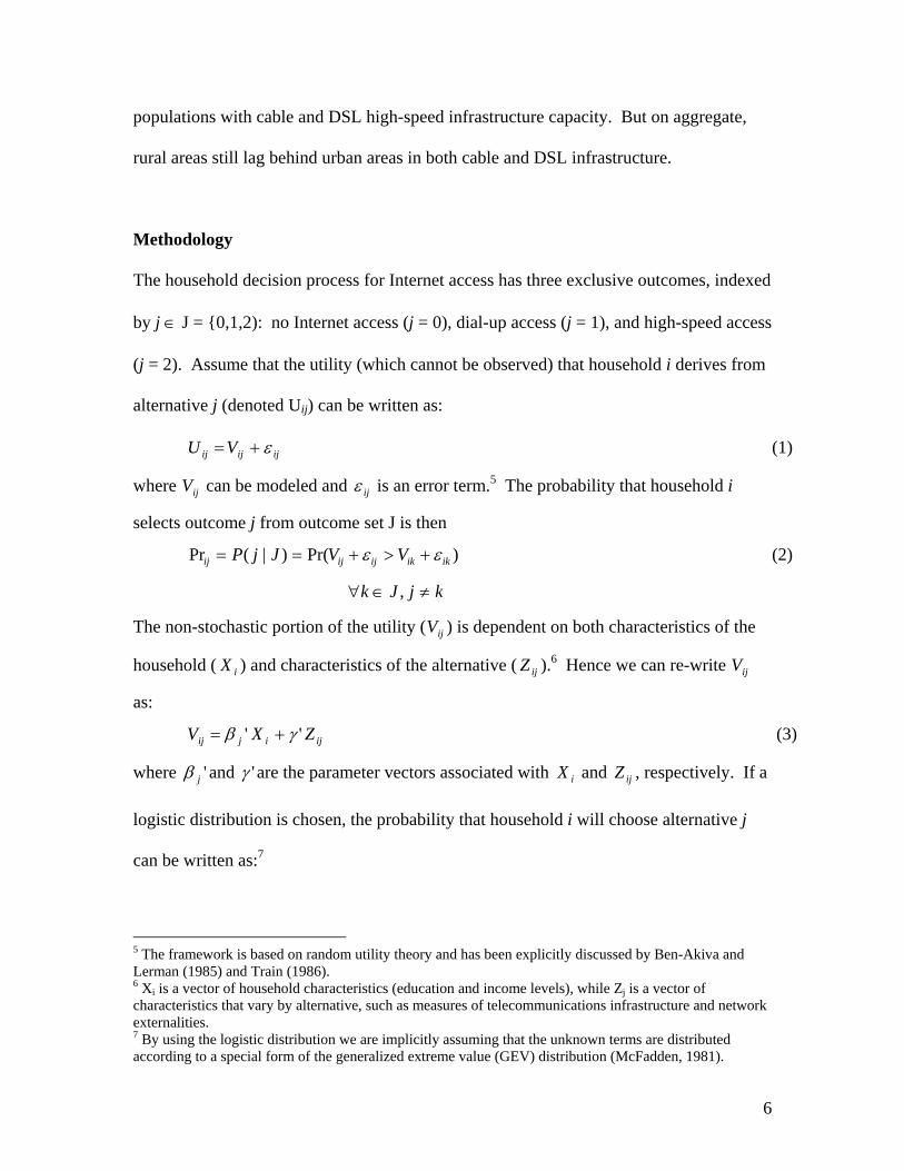
Methodology

The household decision process for Internet access has three exclusive outcomes, indexed

by j ∈ J = {0,1,2): no Internet access (j = 0), dial-up access (j = 1), and high-speed access

(j = 2). Assume that the utility (which cannot be observed) that household i derives from

alternative j (denoted Uij) can be written as:

ijijij VU ε+= (1)

where can be modeled and ijV ijε is an error term.5 The probability that household i

selects outcome j from outcome set J is then

)Pr()|(Pr ikikijijij VVJjP εε +>+== (2)

kjJk ≠∈∀ ,

The non-stochastic portion of the utility ( ) is dependent on both characteristics of the

household ( ) and characteristics of the alternative ( ).

ijV

iX ijZ 6 Hence we can re-write

as:

ijV

ijijij ZXV '' γβ += (3)

where 'jβ and 'γ are the parameter vectors associated with and , respectively. If a

logistic distribution is chosen, the probability that household i will choose alternative j

can be written as:

iX ijZ

7

5 The framework is based on random utility theory and has been explicitly discussed by Ben-Akiva and Lerman (1985) and Train (1986). 6 Xi is a vector of household characteristics (education and income levels), while Zj is a vector of characteristics that vary by alternative, such as measures of telecommunications infrastructure and network externalities. 7 By using the logistic distribution we are implicitly assuming that the unknown terms are distributed according to a special form of the generalized extreme value (GEV) distribution (McFadden, 1981).

6

( )∑∈

=

Jkik

ijij V

VP

exp)exp(

for all j ∈ J (4)

The probabilities shown in equation (4) are those for the multinomial logit model. The

distinctive characteristic of the multinomial logit model is that it assumes the

independence of irrelevant alternatives (IIA). Simply stated, IIA implies that if only two

choices existed (say, no access or dial-up access), then the addition of a third choice

(high-speed access) would not change the ratios of probabilities of the first two choices.

Put another way, the pool of high-speed users would be drawn equally from those with no

access and dial-up access. The nested logit model, however, allows the IIA restriction to

be relaxed and permits dial-up and high-speed access to be modeled as closer substitutes

with each other than with the no access decision.

The two-level nested decision depicted in Figure 2 entails a slightly more complicated

specification of the probability of household i selecting access type j. The joint

probability of a household selecting branch k and twig j is:

Pr [branch k, twig j] ( )( )kkjkj PPP |== . (5)

The conditional probability is defined as

,)exp(

1exp

| ∑∈

⎟⎟⎠

⎞⎜⎜⎝

⎛

=

kJll

jk

kj V

VP

τ (6)

where kτ represents the degree of similarity between the alternatives in branch k. The

marginal probability of selecting branch k is equal to

7

( )( ) .

expexp

∑∈

=

Kkkk

kkk IV

IVP

ττ

(7)

For the kth branch, ,)1exp(ln ∑∈

=kJj

jk

k VIVτ

(8)

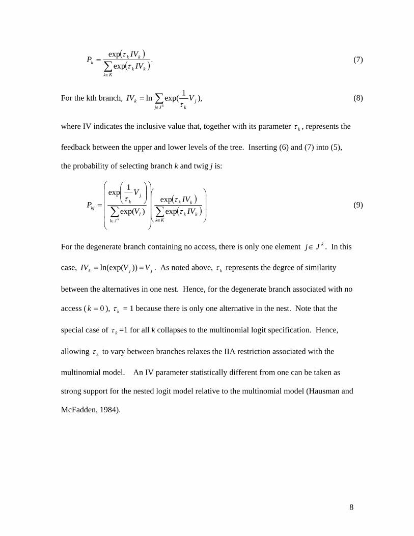
where IV indicates the inclusive value that, together with its parameter kτ , represents the

feedback between the upper and lower levels of the tree. Inserting (6) and (7) into (5),

the probability of selecting branch k and twig j is:

( )( )⎟

⎟⎟

⎠

⎞

⎜⎜⎜

⎝

⎛

⎟⎟⎟⎟⎟

⎠

⎞

⎜⎜⎜⎜⎜

⎝

⎛⎟⎟⎠

⎞⎜⎜⎝

⎛

=∑∑∈∈ Kk

kk

kk

Jll

jk

kj IVIV

V

VP

k

τττ

expexp

)exp(

1exp (9)

For the degenerate branch containing no access, there is only one element . In this

case, . As noted above,

kJj ∈

jjk VVIV == ))ln(exp( kτ represents the degree of similarity

between the alternatives in one nest. Hence, for the degenerate branch associated with no

access ( ), 0=k kτ = 1 because there is only one alternative in the nest. Note that the

special case of kτ =1 for all k collapses to the multinomial logit specification. Hence,

allowing kτ to vary between branches relaxes the IIA restriction associated with the

multinomial model. An IV parameter statistically different from one can be taken as

strong support for the nested logit model relative to the multinomial model (Hausman and

McFadden, 1984).

8

Results

Nested logit model parameter estimates from 2003 are presented in Table 3. Results for

2000 and 2001 are also included in appendix tables A.1 and A.2. Due to the similarity of

the results across all three years, the following discussion will focus only on 2003 (Table

3). Interpretation of nested logit results requires that one potential outcome is selected as

the “default” (McFadden, 1973). With dial-up access arbitrarily selected as this default

category, all coefficients for a characteristic group should be interpreted as relative to a

"default household" – that is, one with the default characteristic value and dial-up

access. The “default household” can be construed from the base characteristics: the

household head did not finish high-school; the household income is less than $5,000; the

head is white and non-Hispanic; is female, single, has no children, and is not retired.

Columns two and three of the table present coefficient estimates for urban households

dealing with the probability of having no access and high-speed access relative to no

access, respectively. Hence, the resulting parameters can be interpreted as the change in

likelihood of either no access or high-speed access relative to dial-up when a

characteristic changes. The fourth and fifth columns present parameter estimates on

interaction terms for rural dummy variables with each characteristic. These coefficients

can be interpreted as rural shifts in the probabilities of no access and high-speed access

relative to dial-up access, respectively.

Model results for 2003 are now discussed with respect to the household characteristic,

place-base characteristic, and infrastructure variable groupings.

9

Household characteristics

Higher levels of education and income decrease the probability of no access relative to

dial-up access. At the same time, higher levels of education and income increase the

probability of high-speed access relative to dial-up, but only at relatively high levels of

education (coll and collplus) and the highest level of income (faminc13). These results

are not surprising given the relationships observed in Table 1. None of the rural

interaction terms for education or income are significant, indicating that the influence of

these characteristics on access is similar in rural and urban areas. Internet access at work

(netatwork) is a significant influence on both no access and high-speed access, with its

presence decreasing the probability of no access and increasing the probability of high-

speed access relative to dial-up access. Furthermore, the interaction of the rural dummy

variable and netatwork is one of the few (weakly) significant interaction terms, with the

positive sign indicating that the presence of Internet access at work is associated with a

higher increase in the propensity for households in rural areas to have high-speed access

than for households in urban areas.

The presence of a Black or Hispanic household head increases the probability of no

access and decreases the probability of high-speed access relative to dial-up, implying

that even after controlling for a multitude of other characteristics race and ethnicity still

play a role in residential Internet access decisions. The presence of a married household

head and between one and three children in the household decreases the probability of no

access relative to dial-up access, but interestingly has no significant effect on high-speed

access. This result is somewhat surprising due to the high-speed nature of many on-line

10

activities for children under 18, such as gaming and music downloading (Horrigan,

2005). Similarly, a retired household head is related to a lower propensity to have no

access relative to dial-up, but has no significant impact on the relative probability of

high-speed access.

Place-based characteristics

Coefficients on local access rates (rate) are strongly significant, implying network

externalities may play an important role in household access decisions. Thus, higher

rates of a distinct type of access in an area (whether it is no access, dial-up, or high-

speed) increase the probability of an individual household obtaining that particular type

of access. Further, the rural interaction terms indicate that the effects of local access rates

are amplified in rural areas.

Digital Communications Technology Infrastructure

The parameter estimates for DCT infrastructure (both DSL and cable) are not

significantly related to any of the relative probabilities of technology use. This is

particularly noteworthy for high-speed access, due to the hypothesized importance of

DCT infrastructure to the high-speed access decision.

It is also worth noting that the IV parameter estimate is significantly different from unity

in all three years, implying the nested logit model is more appropriate than the

multinomial specification.

11

Model Decomposition

A generalized extension of Nielson's (1998) decomposition technique is implemented to

isolate the impact of rural-urban parameter estimate differences, and directly test the

contributions of various characteristics to the rural – urban high-speed digital divides. To

generate the decomposition, equation (9) dealing with the nested logit probability of

choosing alternative j is rewritten as:

],,[)exp(

)exp()exp(

1expτβ

τττ

XFIV

IVV

VP j

Kkkk

kk

Jll

jk

kj

k

=⎟⎟⎟

⎠

⎞

⎜⎜⎜

⎝

⎛

⎟⎟⎟⎟⎟

⎠

⎞

⎜⎜⎜⎜⎜

⎝

⎛⎟⎟⎠

⎞⎜⎜⎝

⎛

=∑∑∈∈

(10)

since utility (Vj) is expressed in terms of X and β. The associated log-likelihood function

then becomes:

]),(,[ln],,[ln)ln(1 2,1,01 2,1,0

τδβτβ ++= ∑ ∑∑ ∑= == =

Rij

N

i jij

Uij

N

i jij XFSXFSL

RU

(11)

where Sij = 1 when household i chooses alternative j, and is 0 otherwise. The superscript

G=(U,R) represents the metropolitan status of household i, is the total number of

households having status G, is a vector of characteristics for household i with status

G., and

GN

GiX

δ is a shift to the parameter β that occurs only for rural households. In order to

assess the roles that the various characteristics play, the following three probabilities are

simulated:

U

N

i

Uij

uj N

XFP

U

∑== 1

]ˆ,ˆ,[ˆ

τβ (12)

12

R

N

i

Rij

rj N

XFP

R

∑=

+= 1

]ˆ),ˆˆ(,[ˆ

τδβ (13)

R

N

i

Rij

rj N

XFP

R

∑== 10

]ˆ,ˆ,[ˆ

τβ (14)

ujP̂ and are the average probabilities of having Internet access equal to type j for urban

and rural households, and will yield the access averages displayed in Figure 1 for rural

and urban areas of the U.S. has no empirical counterpart, and is a simulated

probability in the decomposition technique. is the average probability of having

Internet access equal to type j for rural households with the parameter vector associated

with urban households. This simulated probability allows us to split the total difference

between rural and urban Internet access for type j into two distinct components:

rjP̂

0ˆrjP

0ˆrjP

)ˆˆ()ˆˆ(ˆˆ 00rjrjrjujrjuj PPPPPP −+−=− . (15)

Equations (12) and (13) indicate that the first term on the right-hand side of equation (15)

uses urban parameters for both rural and urban households, and hence isolates differences

in attributes (or characteristics) between households in rural and urban areas. Similarly,

equations (13) and (14) indicate that the second term isolates differences in

underlying parameters between the rural and urban groups.

)ˆˆ( 0rjrj PP −

By changing the vectors and to include different factors associated with the

digital divide, the importance associated with each factor can be assessed in the term

. The initial decomposition will use = = 1, so that no household

UiX R

iX

)ˆˆ( 0rjuj PP − U

iX RiX

13

characteristics are included – thus, with no differences in characteristics, will equal

. Equation (15) then simplifies to and the parameter will account for all

rural – urban differences in the various types of access. Next, models will include a

factor (for instance, education levels of all households), so that does not equal .

Hence, when is calculated, the education characteristics of rural households are used,

along with the parameter vector associated with urban households. Thus, the term

will indicate how much of the divide for type j is due to differences in

education levels between the two areas. The "leftover" portion of the divide still

associated with the parameter vector should become smaller if the rural – urban

differences in explanatory variables are an important factor in the divide. Table 4

displays this sequential decomposition of the nested logit model in tabular form.

ujP̂

0ˆrjP )ˆˆ( 0

rjrj PP − δ̂

UiX R

iX

0ˆrjP

)ˆˆ( 0rjuj PP −

δ̂

One issue with this decomposition technique is the sensitivity of the results to the

ordering in which the dependent variables enter the analysis (due to the non-linearity of

the nested logit functional form). To account for this, several re-orderings of

specifications (2) through (6) in Table 4 will be performed, and the resulting

decompositions will be compared.

Decomposition results for the years 2003, 2001, and 2000 are shown in Table 5. The first

two lines indicate the urban ( ) and rural ( ) average rates of type j access for the

given year, with the third line showing the “digital divide” for the relevant type of access.

One group of explanatory variables is introduced at a time, starting with education levels.

ujP̂ rjP̂

14

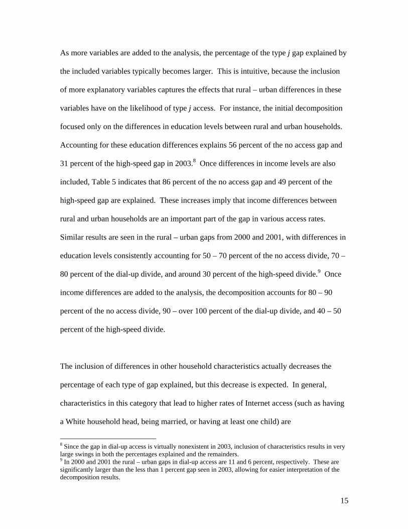
As more variables are added to the analysis, the percentage of the type j gap explained by

the included variables typically becomes larger. This is intuitive, because the inclusion

of more explanatory variables captures the effects that rural – urban differences in these

variables have on the likelihood of type j access. For instance, the initial decomposition

focused only on the differences in education levels between rural and urban households.

Accounting for these education differences explains 56 percent of the no access gap and

31 percent of the high-speed gap in 2003.8 Once differences in income levels are also

included, Table 5 indicates that 86 percent of the no access gap and 49 percent of the

high-speed gap are explained. These increases imply that income differences between

rural and urban households are an important part of the gap in various access rates.

Similar results are seen in the rural – urban gaps from 2000 and 2001, with differences in

education levels consistently accounting for 50 – 70 percent of the no access divide, 70 –

80 percent of the dial-up divide, and around 30 percent of the high-speed divide.9 Once

income differences are added to the analysis, the decomposition accounts for 80 – 90

percent of the no access divide, 90 – over 100 percent of the dial-up divide, and 40 – 50

percent of the high-speed divide.

The inclusion of differences in other household characteristics actually decreases the

percentage of each type of gap explained, but this decrease is expected. In general,

characteristics in this category that lead to higher rates of Internet access (such as having

a White household head, being married, or having at least one child) are

8 Since the gap in dial-up access is virtually nonexistent in 2003, inclusion of characteristics results in very large swings in both the percentages explained and the remainders. 9 In 2000 and 2001 the rural – urban gaps in dial-up access are 11 and 6 percent, respectively. These are significantly larger than the less than 1 percent gap seen in 2003, allowing for easier interpretation of the decomposition results.

15

disproportionately found in rural households. Hence, including these characteristics will

tend to increase the synthetic rates ( ), which in turn will shrink the amount of the rural

– urban gap explained.

0r̂jP

A dramatic increase in the percentage of the rural – urban gap explained for each type of

access occurs when the measures of network externalities are included. In each year, the

percentage of each type of access explained increases by approximately 30 – 50

percentage points after the inclusion of network externalities. This dramatic increase

provides additional evidence that the likelihood of type j access for an individual

household is affected by regional variations in access rates. On the other hand, the

inclusion of differences in DCT infrastructure increases the percentage of the high-speed

gap explained by less than 12 percentage points in each of the three years included in the

analysis. This increase is small compared to other changes (such as the inclusion of

education or network externalities). It is also worth noting that parameter estimates

underlying the decomposition are not statistically significant.

Due to the non-linear nature of the nested logit model, the order in which the variables

were introduced may influence the results. Table 6 accounts for this by reversing the

order in which the variables enter the analysis. Changing the order that the

characteristics enter the analysis does have an effect on the magnitude of the resulting

percentages of the rural – urban gap explained. This "ordering effect" is particularly

notable in the reduced role of education differences and the increased role of DCT

infrastructure differences (for 2000 and 2001) under the reordering. The reordering also

16

has little effect on the increase in the percentage of the gap explained when income and

network externalities were introduced into the analysis. Accounting for income and

network externality differences between rural and urban areas consistently has large

impacts on both dial-up and high-speed rural – urban divides regardless of the order of

the decomposition. This result is highlighted in Table 7, where the impact of introducing

each variable group separately is reported. Under this experiment, the impact of rural –

urban differences in DCT infrastructure remains small for all years of the analysis, never

explaining more than 8 percent of any type of divide. The impact of network

externalities becomes larger, however, explaining over 57 percent of the high-speed

divide and over 86 percent of the no-access divide in any year.

Discussion and Policy Implications

As the nation trends towards Internet connections with higher speeds, concerns continue

to exist that communities with low levels of participation in the information revolution

will lag behind their more connected counterparts, in terms of both economic well-being

and in access to economic opportunities. Historically, the primary course of action of the

federal, state, and local governments to address this concern has been to provide DCT

infrastructure subsidies in low-density regions (Leighton, 2001; Kruger, 2005).

However, decomposition results for the nested logit model of dial-up and high-speed

access suggests that rural – urban differences in income levels and aggregate regional

high-speed access rates are the driving forces behind the high-speed divide, while rural –

urban differences in DCT infrastructure levels are relatively unimportant. These results

(particularly the weak contribution of DCT infrastructure to the divide) imply that efforts

17

to close the emerging rural – urban divide in high-speed access must recognize the rural –

urban income and education gaps that are important underlying factors in the divide,

rather than focusing solely on increasing initiatives for DCT infrastructure investments in

rural areas.

From a policy standpoint, the ultimate rationale for government intervention is to

coordinate positive externalities that would not result from individual household choices.

The estimated existence of strong network externalities suggests such a coordinating role

does exist, as market forces alone may not provide the optimal levels of service.

Consumers are more likely to demand residential access if there are more people to

interact with or ways to use the technology. In turn, suppliers are more likely to provide

infrastructure if there are more users. This is particularly true for high-speed access due

to the expenses involved in providing infrastructure and the multitude of on-line

experiences available to high-speed users. In this light the best policies to reach

households with lower access rates (for the purposes of this study, those in rural areas)

should focus on inducing demand, potentially by subsidizing access and promoting

community networks. Further research may need to identify the "tipping point" where

the impact of such subsidies is largest.

The minimal contribution of differences in DCT infrastructure between rural and urban

areas does not mean that future policies should completely forsake promoting

infrastructure in rural areas. It simply implies that other factors – namely, differences in

18

levels of income and network externalities – are potentially more important in

determining high-speed access rates and need to be included in the policy portfolio.

19

References

Ben-Akiva, M. and S. Lerman. 1985. Discrete Choice Analysis: Theory and Application to Travel Demand. Cambridge, MA: MIT Press.

Cooper, M and G. Kimmelman. 1999. “The Digital Divide Confronts the

Telecommunications Act of 1996.” Consumer Federation of America: Washington D.C.

Drabenstott, M. 2001. “New Policies for a New Rural America.” International

Regional Science Review. 24, 1:3-15. Federal Communications Commission – Industry Analysis and Technology Division.

2003. High Speed Services for Internet Access: Status as of June 30, 2003. Available at http://www.fcc.gov/wcb/iatd/comp.html

Forestier, E., J. Grace, and C. Kenney. 2002. “Can information and communication

technologies be pro-poor?” Telecommunications Policy. 26: 623-646. Graham, S. and A. Aurigi. 1997. “Virtual Cities, Social Polarization, and the Crisis in

Urban Public Space.” Journal of Urban Technology 4:19-52. Grubesic, T. and A. Murray. 2004. “Waiting for Broadband: Local Competition and the

Spatial Distribution of Advanced Telecommunication Services in the United States.” Growth and Change. 35: 2, 139-165.

Hausman, J. and D. McFadden. 1984. "Specification Tests for the Multinomial Logit

Model." Econometrica. 52,5: 1219 – 1240. Hensher, D. and W. Greene. 2000. "Specification and Estimation of the Nested Logit

Model: Alternative Normalizations." Mimeo, New York University. Horrigan, J.B. 2001. Online Communities: Networks that Nurture Long-Distance

Relationships and Local Ties. Pew Internet & American Life Project. http://pewinternet.org/

Horrigan, J.B. 2005. Broadband Adoption at Home in the United States: Growing but

Slowing. Pew Internet & American Life Project. http://pewinternet.org/ Kruger, L. 2005. "Broadband Internet Access and the Digital Divide: Federal

Assistance Programs." Congressional Research Service – The Library of Congress.

Leighton, W.A. 2001. “Broadband Deployment and the Digital Divide.” Cato Policy

Analysis No. 410. August 7.

20

http://www.fcc.gov/wcb/iatd/comp.html

http://pewinternet.org/

http://pewinternet.org/

21

Malecki, E.J. 2003. "Digital Development in rural areas: potentials and pitfalls." Journal of Rural Studies 19: 201-214.

McConnaughey, J., and W. Lader. 1998. Falling Through the Net II: New Data on the

Digital Divide. National Telecommunications and Information Administration, http://www.ntia.doc.gov/ntiahome/net2/falling.html

McFadden, D. 1973. "Conditional Logit Analysis of Qualitative Choice Behavior," in P.

Zarembka, ed., Frontiers in Econometrics. Academic Press: New York McFadden, D. 1981. Econometric Models of Probabilistic Choice. In Structural

Analysis of Discrete Data and Econometric Applications, eds. C.F. Manski and D.L. McFadden, 198-272. Cambridge, MA: MIT Press.

Mills, B.F. and B. Whitacre. 2003. "Understanding the Non-Metropolitan – Metropolitan

Digital Divide." Growth and Change. 34,2: 219-243. National Telecommunications and Information Administration and Economics Statistics

Administration. 2002. How Americans Are Expanding Their Use of the Internet. U.S. Department of Commerce: Washington, D.C.

Nielson, H.S. 1998. "Discrimination and Detailed Decomposition in a Logit Model."

Economics Letters. 61: 115-120. Rose, R. 2003. Oxford Internet Survey Results. The Oxford Internet Institute: The

University of Oxford, UK. Townsend, A. 2001. "The Internet and the Rise of the New Network Cities, 1969 -

1999." Environment and Planning B: Planning and Design, 28: 39-58. Train, K. 1986. Qualitative Choice Analysis. Cambridge, MA: MIT Press.

http://www.ntia.doc.gov/ntiahome/net2/falling.html

22

0

10

20

30

40

50

60

70

Per

cent

of H

ouse

hold

s

Rural - High-speedRural - Dial-upUrban - High-speedUrban - Dial-up

2000 2001 20030

10

20

30

40

50

60

70

Per

cent

of H

ouse

hold

s

Rural - High-speedRural - Dial-upUrban - High-speedUrban - Dial-up

2000 2001 2003

Figure 1. The Shifting Rural - Urban Digital Divide

Figure 2. Nested Logit Tree Structure

Branches

Twig

k ∈ {0,1}

j ∈ {0,1,2}No access Dial-up High-speed

k = 0

j = 1 j = 2j = 0

k = 1 Branches

Twig

k ∈ {0,1}

j ∈ {0,1,2}No access Dial-up High-speed

k = 0

j = 1 j = 2j = 0

k = 1

23

Table 1. Household Characteristics by Type of Internet Access

No Access Dial-up Access High-Speed Access

2000 2001 2003 2000 2001 2003 2000 2001 2003Income

< $25,000 0.463 0.510 0.510 0.124 0.136 0.162 0.089 0.101 0.113$25,001 - $50,000 0.425 0.421 0.423 0.322 0.339 0.368 0.265 0.247 0.250> $50,001 0.214 0.179 0.170 0.595 0.574 0.522 0.675 0.681 0.669

EducationNo High School 0.233 0.253 0.257 0.037 0.049 0.054 0.034 0.030 0.031High School 0.354 0.365 0.373 0.208 0.230 0.251 0.158 0.170 0.171Some College 0.242 0.242 0.235 0.312 0.316 0.321 0.292 0.304 0.290College or More 0.171 0.141 0.135 0.444 0.404 0.375 0.515 0.496 0.508

Race / EthnicityWhite 0.797 0.793 0.780 0.884 0.873 0.865 0.888 0.870 0.859Black 0.166 0.174 0.169 0.066 0.079 0.082 0.060 0.066 0.067Other 0.037 0.033 0.051 0.050 0.048 0.053 0.052 0.064 0.074Hispanic 0.118 0.126 0.149 0.050 0.058 0.073 0.045 0.051 0.062

HH CompositionMarried 0.450 0.401 0.394 0.678 0.667 0.641 0.670 0.660 0.660Male 0.511 0.487 0.489 0.610 0.582 0.559 0.648 0.623 0.603Age of Head 50.5 51.7 51.3 44.1 44.7 46.3 42.9 42.9 43.6# Children 0.477 0.470 0.467 0.475 0.772 0.711 0.487 0.774 0.761

EmploymentEmployed 0.600 0.549 0.529 0.805 0.793 0.744 0.825 0.801 0.797Net at work 0.122 0.137 0.117 0.292 0.415 0.349 0.379 0.505 0.464

Sources: CPS Computer and Internet Use Supplements, 2000, 2001, and 2003.

24

Table 2. Percent of Rural / Urban Population with DCT Infrastructure Capacity

2000 2001 2003Cable

Rural 4.66 5.47 44.10Urban 25.08 27.68 75.75

DSLRural 3.43 6.39 29.55Urban 21.61 32.05 42.39

Sources: Cable Television Factbook, NECA Tariff #4 Data for 2000, 2001, and 2003.

This table assumes that if the infrastructure exists within a rural or urban county (or city), the population of that county (or city) has infrastructure capacity.

25

Table 3. Nested Logit Results (2003) Variables Urban Rural

None Highspeed None Highspeedconstant 1.0559 ** -1.1814 0.0771 -0.7472hs -0.6386 *** 0.0526 0.0503 0.0050scoll -1.3375 *** 0.2028 0.1515 0.1731coll -1.6842 *** 0.3871 * 0.1335 -0.0376collplus -1.8546 *** 0.4027 ** 0.1853 0.1080faminc1 0.2913 -0.3959 -0.3608 1.0742faminc2 0.4053 -0.4137 -0.3092 0.5577faminc3 0.2085 -0.4363 -0.3117 0.8844faminc4 0.2256 -0.5061 -0.4576 1.0108faminc5 0.0957 -0.4796 -0.4391 1.0317faminc6 -0.1136 -0.3570 -0.3463 0.6927faminc7 -0.1795 -0.2086 -0.4451 0.4246faminc8 -0.3407 *** -0.3615 -0.4537 0.7753faminc9 -0.4997 *** -0.5148 -0.6360 1.3911faminc10 -0.8418 *** -0.2525 -0.2627 0.6280faminc11 -0.9836 *** -0.1142 -0.5125 0.6383faminc12 -1.3348 *** -0.0872 -0.1925 0.8989faminc13 -1.7958 *** 0.3647 ** -0.0634 0.6222netatwork -0.5698 *** 0.1357 ** -0.0558 0.0088 *black 0.7308 *** -0.1901 * -0.1170 0.3095othrace 0.1435 0.0680 0.0162 0.6222hisp 0.7381 *** -0.1386 * -0.2782 -0.0619peage -0.0538 ** -0.0043 * -0.0149 -0.0187age2 0.0008 -0.0001 0.0002 0.0003sex -0.0882 0.1855 0.1726 -0.2229married -0.5024 ** -0.0349 -0.0991 -0.1952chld1 -0.2558 *** -0.0279 -0.0107 0.3900chld2 -0.3010 *** -0.0305 -0.0167 0.3049chld3 -0.1757 ** -0.1397 0.0225 0.4133chld4 -0.2211 -0.2889 0.5778 0.2635chld5 -0.1249 -0.2058 -0.0894 -0.2093retired -0.1223 *** -0.0789 -0.3006 0.3487rate 2.7352 *** 2.2806 *** 0.5027 * 2.8191 **dslaccess -0.1544 0.2099 0.0402 -0.1538cableaccess -0.2525 0.4210 0.3713 -0.5937

IV - no 1IV - yes 0.8920 ***

Log-likelihood -17632.0Note: *, ***, and *** indicate statistically significant differences from zero at the p = 0.10, 0.05, and 0.01 levels, respectively. For the inclusive value (IV), they indicate a statistically significant difference from one.

26

27

Table 4. Decomposition of Nested Logit Specification

Specification Explanatory VariablesVariables

AddedDifferences in

AttributesDifferences in

Parameters(1) Constant term 0 rural intercept (δ)(2) (1) + Education Levels XE XE rural intercept (δ)(3) (2) + Income Levels XI XE + XI rural intercept (δ)(4) (3) + Other Household Characteristics XO XE + XI + XO rural intercept (δ)(5) (4) + Network Externalities XN XE + XI + XO + XN rural intercept (δ)(6) (5) + DCT Infrastructure XT XE + XI + XO + XN + XT rural intercept (δ)

Hypotheses: δ(1) > δ(2) > δ(3) > δ(4) > δ(5) > δ(6) for dial-up and high-speed accesspeed access > Importance of XT for dial-up access

Ri

Ui XX = )ˆˆ( 0

rjuj PP − )ˆˆ( 0rjrj PP −

)ˆˆ( rjuj PP −

Importance of XT for high-s

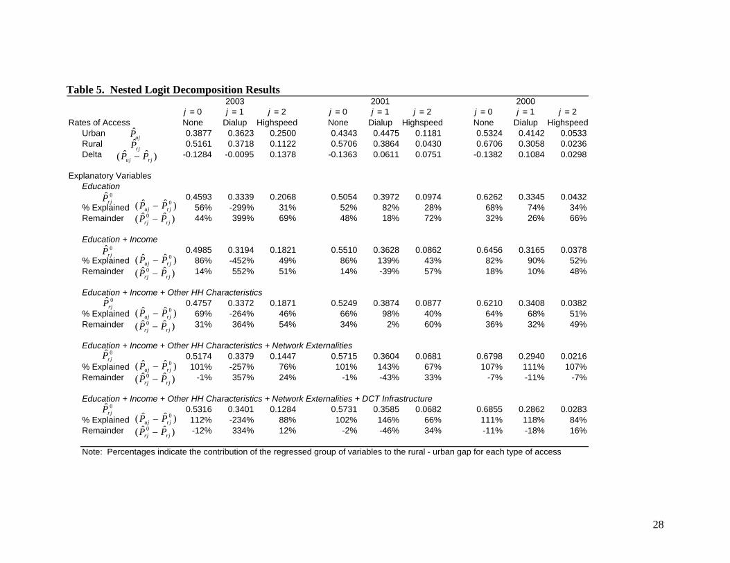
Table 5. Nested Logit Decomposition Results 2003 2001 2000

j = 0 j = 1 j = 2 j = 0 j = 1 j = 2 j = 0 j = 1 j = 2Rates of Access None Dialup Highspeed None Dialup Highspeed None Dialup Highspeed

Urban 0.3877 0.3623 0.2500 0.4343 0.4475 0.1181 0.5324 0.4142 0.0533Rural 0.5161 0.3718 0.1122 0.5706 0.3864 0.0430 0.6706 0.3058 0.0236Delta -0.1284 -0.0095 0.1378 -0.1363 0.0611 0.0751 -0.1382 0.1084 0.0298

Explanatory VariablesEducation

0.4593 0.3339 0.2068 0.5054 0.3972 0.0974 0.6262 0.3345 0.0432% Explained 56% -299% 31% 52% 82% 28% 68% 74% 34%Remainder 44% 399% 69% 48% 18% 72% 32% 26% 66%

Education + Income0.4985 0.3194 0.1821 0.5510 0.3628 0.0862 0.6456 0.3165 0.0378

% Explained 86% -452% 49% 86% 139% 43% 82% 90% 52%Remainder 14% 552% 51% 14% -39% 57% 18% 10% 48%

Education + Income + Other HH Characteristics0.4757 0.3372 0.1871 0.5249 0.3874 0.0877 0.6210 0.3408 0.0382

% Explained 69% -264% 46% 66% 98% 40% 64% 68% 51%Remainder 31% 364% 54% 34% 2% 60% 36% 32% 49%

Education + Income + Other HH Characteristics + Network Externalities0.5174 0.3379 0.1447 0.5715 0.3604 0.0681 0.6798 0.2940 0.0216

% Explained 101% -257% 76% 101% 143% 67% 107% 111% 107%Remainder -1% 357% 24% -1% -43% 33% -7% -11% -7%

Education + Income + Other HH Characteristics + Network Externalities + DCT Infrastructure0.5316 0.3401 0.1284 0.5731 0.3585 0.0682 0.6855 0.2862 0.0283

% Explained 112% -234% 88% 102% 146% 66% 111% 118% 84%Remainder -12% 334% 12% -2% -46% 34% -11% -18% 16%

Note: Percentages indicate the contribution of the regressed group of variables to the rural - urban gap for each type of access

ujP̂rjP̂

)ˆˆ( rjuj PP −

0ˆrjP

)ˆˆ( 0rjuj PP −

)ˆˆ( 0rjrj PP −

0ˆrjP

0ˆrjP

0ˆrjP

0ˆrjP

)ˆˆ( 0rjuj PP −

)ˆˆ( 0rjrj PP −

)ˆˆ( 0rjuj PP −

)ˆˆ( 0rjrj PP −

)ˆˆ( 0rjuj PP −)ˆˆ( 0

rjrj PP −

)ˆˆ( 0rjuj PP −

)ˆˆ( 0rjrj PP −

28

Table 6. Nested Logit Decomposition Results (Order Reversed) 2003 2001 2000



Explanatory VariablesDCT Infrastructure

0.3985 0.3999 0.2417 0.4405 0.4447 0.1148 0.5434 0.4058 0.0508% Explained 8% 396% 6% 5% 5% 4% 8% 8% 8%Remainder 92% -296% 94% 95% 95% 96% 92% 92% 92%

DCT Infrastructure + Network Externalities0.4585 0.3331 0.1875 0.4850 0.4018 0.0752 0.6004 0.3459 0.0428


DCT Infrastructure + Network Externalities + Other HH Characteristics0.4492 0.3405 0.1957 0.4805 0.4106 0.0852 0.5924 0.3511 0.0435


DCT Infrastructure + Network Externalities + Other HH Characteristics + Income0.5014 0.3383 0.1502 0.5685 0.3785 0.0724 0.6739 0.2988 0.0285

% Explained 89% -253% 72% 98% 113% 61% 102% 106% 83%Remainder 11% 353% 28% 2% -13% 39% -2% -6% 17%

DCT Infrastructure + Network Externalities + Other HH Characteristics + Income + Education0.5316 0.3401 0.1284 0.5731 0.3585 0.0682 0.6855 0.2862 0.0283

% Explained 112% -234% 88% 102% 146% 66% 111% 118% 84%Remainder -12% 334% 12% -2% -46% 34% -11% -18% 16%


ujP̂rjP̂

)ˆˆ( rjuj PP −

0ˆrjP

)ˆˆ( 0rjuj PP −

)ˆˆ( 0rjrj PP −

0ˆrjP

0ˆrjP

0ˆrjP

0ˆrjP

)ˆˆ( 0rjuj PP −

)ˆˆ( 0rjrj PP −

)ˆˆ( 0rjuj PP −

)ˆˆ( 0rjrj PP −

)ˆˆ( 0rjuj PP −)ˆˆ( 0

rjrj PP −

)ˆˆ( 0rjuj PP −

)ˆˆ( 0rjrj PP −

)ˆˆ( 0rjuj PP −

)ˆˆ( 0rjuj PP − )ˆˆ( 0rjuj PP −

29

30

Table 7. Nested Logit Decomposition Results (Single Explanatory Variables) 2003 2001 2000



Explanatory VariablesEducation

0.4593 0.3339 0.2068 0.5054 0.3972 0.0974 0.6262 0.3345 0.0432% Explained 56% -299% 31% 52% 82% 28% 68% 74% 34%Remainder 44% 399% 69% 48% 18% 72% 32% 26% 66%

Income0.4792 0.3271 0.1937 0.5337 0.3764 0.0899 0.6031 0.3536 0.0432


Other HH Characteristics0.3999 0.3642 0.2359 0.4502 0.4384 0.1113 0.5370 0.4123 0.0507

% Explained 10% 20% 10% 12% 15% 9% 3% 2% 9%Remainder 90% 80% 90% 88% 85% 91% 97% 98% 91%

Network Externalities0.4987 0.3213 0.1589 0.5598 0.3810 0.0751 0.6638 0.3055 0.0306


DCT Infrastructure 0.3985 0.3999 0.2417 0.4405 0.4447 0.1148 0.5434 0.4058 0.0508

% Explained 8% 396% 6% 5% 5% 4% 8% 8% 8%Remainder 92% -296% 94% 95% 95% 96% 92% 92% 92%


ujP̂rjP̂

)ˆˆ( rjuj PP −

0ˆrjP

)ˆˆ( 0rjuj PP −

)ˆˆ( 0rjrj PP −

0ˆrjP

0ˆrjP

0ˆrjP

0ˆrjP

)ˆˆ( 0rjuj PP −

)ˆˆ( 0rjrj PP −

)ˆˆ( 0rjuj PP −

)ˆˆ( 0rjrj PP −

)ˆˆ( 0rjuj PP −

)ˆˆ( 0rjrj PP −

)ˆˆ( 0rjuj PP −

)ˆˆ( 0rjrj PP −

)ˆˆ( 0rjuj PP −

)ˆˆ( 0rjuj PP − )ˆˆ( 0rjuj PP −

Appendix A.1 – Nested Logit Results (2000) Variables Urban Rural

None Highspeed None Highspeedconstant 0.1260 *** -1.9091 *** 0.5125 -0.6490 *hs -0.5362 *** -0.3194 -0.2175 0.6751scoll -1.1582 *** -0.1760 -0.4571 0.8483coll -1.4914 *** 0.0697 -0.4524 0.5560collplus -1.6087 *** 0.1718 ** -0.4938 1.0592faminc1 0.2509 -0.0881 0.4216 -3.0757faminc2 0.2470 -0.1239 0.1711 -1.7583faminc3 0.1378 -0.2198 0.3059 -0.1288faminc4 -0.1648 -0.0878 0.0903 -1.3618faminc5 -0.0154 -0.6346 -0.2994 0.5055faminc6 -0.1920 -0.1627 0.0355 -0.2920faminc7 -0.5420 ** 0.1353 0.2438 -0.8961faminc8 -0.7451 *** 0.1630 0.1296 -0.9369faminc9 -0.6096 *** -0.2381 -0.0758 0.0505faminc10 -0.9662 *** 0.0334 -0.0389 -0.1034faminc11 -1.1606 *** 0.1810 0.1348 -0.8307faminc12 -1.4247 *** 0.1661 ** 0.1841 -0.6850faminc13 -1.9408 *** 0.4329 *** 0.1434 -0.3838netatwork -0.1984 *** 0.2505 ** 0.2269 -0.0660black 0.9197 *** -0.2478 * -0.1509 0.1654othrace 0.1407 -0.1198 0.5257 -1.2931hisp 0.7761 *** -0.1058 ** 0.0749 -0.0633peage -0.0329 ** -0.0145 -0.0179 -0.0248age2 0.0006 0.0001 0.0001 0.0004sex -0.0525 0.1002 * 0.0288 0.3372married -0.3799 ** -0.1381 -0.1113 -0.3665chld1 0.0410 0.1461 -0.0055 -0.3612chld2 -0.0260 0.1127 0.0678 -0.0338chld3 0.1391 0.0641 -0.0833 -0.2163chld4 -0.2051 -0.0784 -0.2254 0.4692chld5 -0.0633 0.3247 0.7138 -4.9407retired -0.0907 *** 0.1535 0.2295 -0.3023rate 3.0846 *** 5.1862 ** 0.5410 * 6.2007dslaccess -0.1811 0.1400 0.1388 0.3283cableaccess 0.0556 -0.1913 -0.7822 * 0.9272

IV - no 1IV - yes 0.9302 **

Log-likelihood: -22,905Note: *, **, and *** indicate statistically significant differences from zero at the p = 0.10, 0.05, and 0.01 levels, respectively. For the inclusive value (IV), theyindicate a statistically significant difference from one.

31

Appendix A.2 – Nested Logit Results (2001)

Variables Urban RuralNone Highspeed None Highspeed

constant 0.9714 *** -1.1705 ** 0.7362 -1.5876 *hs -0.6216 *** 0.0907 0.0040 0.0657scoll -1.1609 *** 0.2458 -0.0080 -0.1385coll -1.4678 *** 0.3243 0.1291 -0.0090collplus -1.5454 *** 0.2218 ** -0.1759 0.0162faminc1 0.2609 -0.6960 0.0352 -1.1593faminc2 0.3295 -0.2356 -0.4138 -0.7735faminc3 0.0644 -0.0669 -0.4968 0.2149faminc4 0.0886 -0.2932 -0.1041 0.6921faminc5 -0.0163 -0.5568 -0.0948 1.1272faminc6 -0.1948 -0.5249 -0.2424 0.1533faminc7 -0.3813 ** -0.4621 -0.1588 0.7051faminc8 -0.6412 *** -0.3996 -0.1982 0.6744faminc9 -0.6943 *** -0.4100 0.0102 0.5392faminc10 -0.8996 *** -0.2938 -0.1582 0.3182faminc11 -1.1025 *** -0.3602 -0.1485 0.8044faminc12 -1.3692 *** -0.1564 -0.0726 0.8517faminc13 -1.8157 *** 0.1291 ** 0.0106 0.5704netatwork -0.4794 *** 0.1548 ** -0.1144 -0.1120black 0.7903 *** -0.1878 ** -0.3079 0.2319othrace -0.0875 0.0345 0.4239 0.5828hisp 0.7048 *** -0.1202 * -0.1332 0.4554peage -0.0377 ** -0.0202 -0.0247 -0.0172age2 0.0006 0.0001 0.0002 0.0003sex 0.0077 0.1770 0.0116 -0.1502married -0.5325 ** -0.1286 -0.1983 0.0135chld1 -0.1893 -0.0081 -0.1385 0.2683chld2 -0.3210 0.0050 -0.1383 -0.3462chld3 -0.2902 0.0575 0.0789 -0.9515chld4 -0.1242 0.0452 -0.1546 -0.2112chld5 -0.2163 -0.0392 0.4633 -0.1191retired -0.0449 *** 0.1479 -0.1235 -0.3828rate 2.3405 *** 3.4180 ** 0.5711 ** 8.2573dslaccess -0.0665 0.1578 -0.2219 -0.4152cableaccess 0.1164 -0.2998 -0.1022 -0.6213

IV - no 1IV - yes 0.8504 ***

Log-likelihood: -29,876Note: *, **, and *** indicate statistically significant differences from zero at the p = 0.10, 0.05, and 0.01 levels, respectively. For the inclusive value (IV), theyindicate a statistically significant difference from one.

32

A Need for Speed

Documents

Transcript of A Need for Speed