A near -global eddy -resolving OGCM for climate studies€¦ · other modelling groups who are...

1

5

A near-global eddy-resolving OGCM for climate studies

X. Zhang1, P. R. Oke1, M. Feng2, M. A. Chamberlain1, J. A. Church1, D. Monselesan1, C. Sun2, R. J.

Matear1, A. Schiller1 and R. Fiedler1

1CSIRO Oceans and Atmosphere, Hobart, TAS, 7001, Australia 10 2CSIRO Oceans and Atmosphere, Floreat, Western Australia, 6014, Australia

Correspondence to: Xuebin Zhang ([email protected])

15

20

25

30

Geosci. Model Dev. Discuss., doi:10.5194/gmd-2016-17, 2016Manuscript under review for journal Geosci. Model Dev.Published: 15 February 2016c© Author(s) 2016. CC-BY 3.0 License.

2

Abstract. Eddy-resolving global ocean models are highly desired for spatially-improved climate studies, but this is challenging

because they require careful configuration and substantial computational resources. Model drift, partially related to insufficient

model spin-up, imperfect model physics or bias in surface forcing, can be problematic, leading to contamination of climate

change signals. In this study, we adapt a near-global eddy-resolving ocean general circulation model, originally developed for

short-range ocean forecasting, for climate studies. The Ocean Forecasting Australia Model version 3 (OFAM3) is spun up for 5

20 years, with repeated year 1979 forcing and adaptive relaxation (Newtonian nudging) of temperature and salinity in the deep

ocean to an observation-based climatology. In addition, surface heat fluxes from the JRA-55 atmospheric reanalysis are

adjusted during the spin-up experiment to minimise excessive net heat uptake in the ocean. In the historical experiment,

spanning 1979-2014, a non-adaptive relaxation is applied by repeating the same relaxation rates derived from the last five

years of the spin-up experiment, and the surface heat flux adjustment diagnosed during the spinup experiment is also 10

maintained. We demonstrate that the historical experiment driven by the JRA-55 reanalysis does not have significant drifts

(e.g., as shown by simulated global ocean heat content), and also provides an eddy-resolving simulation of the global ocean

circulation over the period 1979-2014. Decadal changes, such as the strengthening of the subtropical gyre circulation, are also

reasonably simulated. A biogeochemical model is coupled with OFAM3 to produce patterns of primary productivity and

carbon fluxes that are consistent with observations. Experiences gained from our numerical experiments will be helpful to 15

other modelling groups who are interested in running global eddy-resolving OGCMs for climate studies.

1 Introduction

Global climate models provide useful information about large-scale climate change and variability in both the past and the

future, as shown in the Fifth Assessment Report of IPCC (2013). With relatively coarse resolution (e.g., 1° in the ocean

component) global climate models are primarily designed to study large-scale climate change and variability over decades to 20

centuries under different climate scenarios. As a result, mesoscale features in the ocean are often absent in global climate

models, however, they are important for studying climate-related variability of ocean boundary currents, eddies, continental

shelf and biogeochemical processes. Mesoscale eddies in the ocean play significant roles in heat transport and exchange

(Griffies et al. 2015), the ocean kinetic energy budget (Ferrari and Wunch 2008; Schiller et al. 2008), and the supply of nutrients

to the upper ocean (McGillicuddy et al. 1998). 25

Noting that the first baroclinic Rossby radius of deformation in the ocean is in the range of 20~200 km, with smaller values

in high latitudes and larger values in low latitudes (e.g., Chelton et al. 1998), the ocean general circulation models (OGCMs),

either as stand-alone ocean models or as ocean components in the coupled climate models, need to have a horizontal resolution

of ¼° to permit mesoscale eddies, and a higher resolution (1/10o or finer) to resolve them. There have been growing efforts to

develop global eddy-permitting and eddy-resolving OGCMs in the past 1-2 decades (e.g., Masumoto et al. 2004; Maltrud and 30

McClean, 2005; Chassignet et al. 2007; Sasaki et al., 2008; Yu et al. 2012; Oke et al. 2013a; Sérazin et al. 2015), often based


3

on experiences gained from setting-up high-resolution basin-scale experiments, e.g., in the North Atlantic (Smith et al. 2000;

McClean 2002).

Despite significant increase of computational power, running a global eddy-resolving model over long periods (e.g., > 50

years), is still a major undertaking. In fact, it’s quite common that global eddy-resolving models are integrated over 1~2

decades only (e.g., Maltrud and McClean 2005; Yu et al. 2012), with a few pioneering efforts to run global eddy-resolving 5

models over several decades (Sasaki et al. 2008; Sérazin et al. 2015; Griffies et al. 2015). However, the integration time needed

for an OGCM to reach thermodynamic equilibrium is much longer (e.g., McWilliams 1996; Griffies et al. 2014). Model drift

is a long-standing problem, not only in ocean-only models, but also in coupled climate models, often caused by insufficient

model spin-up (e.g., Sen Gupta et al. 2012, 2013; Griffies et al. 2014; Hobbs et al. 2016). For example, in the suite of

Coordinated Ocean-ice Reference Experiments - Phase II (CORE-II) models, with typical grid resolution of 1° (Griffies et al. 10

2014), drifts can persist in some of models even after 300 years of integration. The changes induced by model drift – a model

artefact, can be comparable to or ever larger than the real climate changes signals under investigation. The model drift therefore

needs to be appropriately understood and quantified (e.g., Sen Gupta et al. 2012, 2013).

In this study, we modify a near-global eddy-resolving OGCM – the Ocean Forecasting Australian Model, Version 3

(OFAM3, Oke et al. 2013a) for climate change applications. OFAM3 and its previous versions (OFAM 1 and OFAM2) were 15

primarily developed for upper-ocean, short-range operational forecasting (Oke et al. 2005; Schiller et al. 2008; Oke et al.

2013b). We implement several practical strategies (e.g., new ways of implementing temperature and salinity relaxation in the

deep ocean, and adjusting surface heat fluxes) to run OFAM3 such that after twenty years of spin up from rest OFAM3 does

not show significant drifts. Moreover, we show that the new configuration realistically simulates the ocean variability over the

period 1979-2014. 20

Including a biogeochemical (BGC) model in OFAM3 enables a simulation of primary productivity (PP), nutrient and carbon

cycling in the ocean. Ocean productivity is expected to decrease with climate change as increasing stratification of the upper

ocean reduces the supply of nutrients (Saramiento et al. 2004). By contrast, previous ocean downscaling of climate projections,

have indicated that productivity can increase locally, due to changes in mesoscale variability (Matear et al. 2013). The

mesoscale resolution of OFAM3 allows us to investigate the interaction of the BGC fields with the ocean physics across the 25

near-global model domain.

The paper is organized as follows. In section 2, OFAM3 (Oke et al. 2013a) is briefly introduced, and details of the innovations

in the new configuration are explained. The spin-up experiment, forced by repeating year 1979 forcing for two decades, is

discussed in Section 3. The historical experiment, over 1979-2014, is described in Section 4. Finally, a discussion and

conclusions are presented in Section 5. 30


4

2 Model setup

As a baseline for this study, we use the most recent OFAM version – OFAM3, described in detail in Oke et al. (2013). In this

section, we provide a short description of the model, and focus on the innovations of the new configuration that are motivated

to make the model more suitable for climate studies.

OFAM3, based on version 4p1d of the Geophysical fluid Dynamics Laboratory Modular Ocean Model (Griffies, 2009), is 5

configured to have 0.1o grid spacing for all longitudes and between 75°S and 75°N (~ 8-11 km x 11 km), comprising 3600x1500

horizontal grid points (Fig. 1). It has 51 vertical layers, with 14 layers between the surface and 100 m depth, 19 layers between

100 and 500 m depth, 6 layers between 500 and 1000 m depth, and 12 layers below 1000 m. A partial cell technique (Adcroft

et al. 1997) is employed to better represent bottom topography.

Horizontal mixing, dependent on model state and grid size, is provided by the biharmonic Smagorinsky viscosity scheme 10

(Griffies and Hallberg 2000), while vertical mixing is provided by K-profile parameterization (KPP, Large et al. 1994), rather

than the scheme by Chen et al. (1994) adopted in a previous OFAM3 configuration. The effect of barotropic tidal mixing is

parameterized by the tidal frictional turbulence, which is combined with the vertical mixing from the KPP (Lee et al. 2006).

The model is forced by 3-hourly Japanese 55-year Reanalysis (JRA-55; Kobayashi et al. 2015). Previous versions of OFAM

used surface fluxes of heat and momentum, derived directly from an atmospheric reanalysis (e.g., Oke et al. 2013a). The new 15

configuration uses bulk formula (Large and Yeager 2004) for wind stress, turbulent sensible and latent fluxes, and evaporation.

Total precipitation is based on the JRA-55 reanalysis, while monthly climatologies of river run-offs are from Dai and

Trenberth (2002) and Dai et al. (2009). The net global freshwater flux (i.e., sum of evaporation, precipitation and river run-

offs) is balanced at each model time step to ensure consistency with the Boussinesq approximation (Gill 1982). Consequently,

the model global ocean volume is conserved and the global mean sea level is always zero (e.g., Griffies et al. 2000). 20

Model drift in ocean properties in forced experiments is common (e.g., Griffies et al. 2014), as a result of missing interactions

with the atmosphere and sea ice, biases in surface forcing, imperfection of model parameterization (e.g., mixing scheme),

inaccurate initial conditions, and long-term adjustment processes such as those associated with the thermohaline circulation.

As a result, relaxation of temperature and salinity to a climatology, particularly in the deep ocean, is often used to reduce drifts

in deep-water properties and to keep the model fields closer to reality. For example, in previous OFAM3 experiments (Oke et 25

al. 2013a), temperature and salinity in the deep ocean (below 2000 m) are weakly relaxed to climatology from the CSIRO

Atlas for Regional Seas (CARS 2009 release; Ridgway and Dunn 2003) with a time-scale of one year.

Relaxation is typically added as an extra forcing term to the temperature or salinity equation in the form of Newtonian

nudging to prevent the model fields from diverging too much from the observed climatology. Such relaxation is adaptive, and

thus depends on the difference between the model state and climatology, with stronger relaxation when differences are larger. 30

Adaptive relaxation represents a time-dependent source or sink of the heat and salt, often obscuring the “true” climate change

signals that are of primary interest. However, due to model shortcomings, relaxation is often a common technique used in

global eddy resolving OGCMs, including previous OFAM experiments (e.g., Oke et al. 2013a). Here we use a new design by


5

applying an appropriate non-adaptive relaxation that will minimise model drift, while also allowing the model to simulate deep

variability. To achieve this, we apply an adaptive relaxation for temperature and salinity during the 20-year spin-up experiment

with repeated year 1979 forcing. We then diagnose a seasonal climatology of it and then repeatedly apply the seasonal

relaxation in a non-adaptive manner (i.e., relaxation doesn’t depend on model state anymore) throughout the historical

experiment. We find that this combination of adaptive relaxation during the spin-up experiment, and non-adaptive relaxation 5

during the historical experiment keeps the deep-ocean close to the observed climatology but allows the climate changes signals

to penetrate to the deep ocean.

In addition to the deep ocean relaxation, temperature and salinity are also relaxed to the CARS climatology from the top to

the bottom within a 5° buffer zone from the northern boundary in the Northern Atlantic to reduce the impacts from a missing

Arctic ocean. Within the boundary buffer zone, the relaxation timescale linearly increases from 30 days at the boundary to 365 10

days in the interior. Sea surface salinity is also weakly restored to monthly CARS climatology with a time-scale of 180 days.

In reality, the ocean areas that are under ice don’t “feel” the atmosphere. However, because OFAM3 does not include a sea-

ice model, the naive application of bulk surface fluxes can lead to problems, e.g., significant heat loss at the surface that triggers

massive convection. A solution to this involves the use of the JRA-55 sea ice coverage field to mask the applied atmospheric

forcing fields. The sea ice coverage field, ranging from 0 (ice-free) to 1 (full-ice), is typically either near 0 or near 1, without 15

extensive intermediate values. Specifically, when the ice cover fraction (a) is greater than 0.1, the air temperature is set to -

1.8 oC – the freezing point of sea water. Additionally, wind speed, downward shortwave radiation, and downward longwave

radiation are scaled by the ice-free fraction (1-a) to give a transition from unmodified atmospheric fields in ice-free conditions,

to zero under complete ice cover. Blackbody radiation at the freezing point is also scaled by ice cover (a*307.4 W m-2). Finally,

the ocean temperature in the model occasionally falls below the freezing point of sea water (-1.8 oC). If this occurs, the 20

temperature is reset to -1.8 oC, a quite common practice for ocean models without an explicit sea ice component (e.g., Yu et

al. 2012).

In addition to the physics, OFAM3 includes the World Ocean Model of Biology and Trophic dynamics (WOMBAT; Oke

et al. 2013a). WOMBAT is based on a simple nutrient, phytoplankton, zooplankton and detritus model, with the addition of

an oxygen and carbon cycle. We include WOMBAT in our climate simulations to enable the investigation into how climate 25

changes impact PP and nutrient and carbon cycling. Oke et al. (2013a) includes a detailed description of WOMBAT. In the

experiment presented here, the BGC parameters used with WOMBAT are based on Oschlies and Schartau (2005), with extra

parameters for the carbon cycle (Law et al. 2015). For the carbon, we include two separate dissolved inorganic tracers: 1)

forced with rising atmospheric CO2 levels (anthropogenic carbon tracer) and 2) forced with atmospheric CO2 of 280ppm

(natural carbon tracer). These parameters differ from the implementation of Oke et al. (2013a), and are intended to improve 30

the BGC behaviour in oligotrophic waters. The model BGC fields are initialised with observations. Specifically, the World

Ocean Atlas is used to initialise nutrients (phosphorus) and oxygen (Garcia et al 2006a; Garcia et al. 2006b). The Global

Ocean Data Analysis Project (GLODAP) product is used to initialise alkalinity and dissolved carbon (Sabine et al. 2004; Key

et al. 2004). Phytoplankton is initialised with SeaWIFS observation (NASA, 2014) and zooplankton is initialised as a fraction


6

of phytoplankton (0.05). We also include a restoring term to the deep-water BGC fields below 2000 m, which is employed to

ensure the deep-water BGC fields remain realistic. These deep fields (nutrients, oxygen, alkalinity, and carbon) are adaptively

relaxed to observations with the same time scale (i.e., one year) and over the same spatial extent as the temperature and salinity

fields (see above) in the spin-up experiment. Inclusion of the BGC component of the system is computationally expensive.

The BGC fields are therefore spun up for only 15-years – followed by integration in the historical run between 1992 and 2014. 5

This duration spans the era of relevant satellite sea-colour observations.

3 Spin-up experiment

The correct spin-up of OGCMs is critical for ocean climate applications, and it is important to provide a realistic initial

condition (IC) for historical experiments. Only over the most recent decade, the global upper ocean (above 2000 m) has been

regularly observed, mainly because of the global Argo float program (Roemmich and Owens 2000), and as a result it became 10

feasible to initialize a model based on in-situ observations. Before the Argo program, it is not a trivial task to get a dynamically

consistent IC for hindcast experiments (e.g., McWilliams 1996).

Considering the needs to spin-up the model and to ensure a reasonable IC for the subsequent climate change simulations,

we start the model from rest with the initial temperature and salinity fields from CARS climatology (2009 release; Ridgway

and Dunn 2003), then apply a repeating normal-year type forcing over a long enough period for the model ocean (at least the 15

upper to middle depths) to stabilize. The year 1979 corresponds to the start year of the historical run, and is also chosen as the

‘normal year’ for the spin-up experiment, because both Pacific Decadal Oscillation (PDO, Mantua and Hare, 2002) and El

Niño Southern Oscillation (ENSO, McPhaden et al., 2006) phases are close to near-neutral. The idea of applying normal-year

forcing was previously used in the CORE-Phase I (CORE-I) experiment (Griffies et al. 2009).

Three-hourly forcing from JRA-55 reanalysis for 1979 is applied repeatedly to spin the ocean up. In the spin-up simulation 20

(referred to as “OFAM3-JRA55-spinup” experiment), the ocean rapidly adjusts in the first couple of years, as indicated by the

evolution of the global mean kinetic energy (Fig. 2) and global mean ocean heat content (OHC) (Fig. 3). The upper ocean

takes only several months for its kinetic energy to reach around ~200 cm2 s-2, and a clear seasonal cycle can be seen from Year

2 of the spin-up experiment (Fig. 2b). In contrast, it takes about two years for the deep layer to reach ~8 cm2 s-2 and stay at a

similar level afterwards (Fig. 2c). The evolution of volume-averaged kinetic energy over the full depth is similar to that of 25

bottom layer, with slightly higher values around 20 cm2 s-2 (Fig. 2a).

In the first two years of the simulation the ocean gains heat at a rate of 17.8 W m-2 and 7.73 W m-2 in Year 1 and Year 2,

respectively (Table 1). If we continue without any heat flux correction, the model ocean state in most regions would develop

a warm bias relative to the CARS climatology. To avoid that, in Year 3 the annual mean net surface heat flux from Year 2

(7.73 W m-2) is removed from the downward longwave radiation. With this heat flux correction, the annual mean net flux in 30

Year 3 is 3.12 W m-2, smaller but non-zero. In Year 4, the sum of the mean net heat flux from both Year 2 (7.73 W m-2) and

Year 3 (3.12 W m-2) is removed from the downward longwave radiation, which leads to a net heat flux of 2.48 W m-2. Repeating


7

this approach each year until Year 7, the net heat flux converges to a smaller value of about 1 W m-2. From Year 8 to Year 20,

the same heat flux correction (-16.925 W m-2) is applied, which resulted in gradually reduced net surface heat flux to below

0.5 W m-2 from Year 15 to Year 20. This value is close to the net surface heat flux (0.4-0.6 W m-2) inferred from Argo

measurements over the 2006-2014 period (Roemmich et al. 2015).

The -16.925 W m-2 heat flux correction is quite large, but is comparable to the large uncertainty and discrepancy of net heat 5

flux from the different atmospheric reanalysis products. For example, the Objectively Analyzed air-sea Fluxes (OAFlux, Yu

and Weller 2007) product which objectively blended several popular atmospheric reanalysis products has a mean net heat flux

of 30 W m-2 over 1983-2009, which is much larger than the <1.0 W m-2 based on observed ocean heat content change in the

past several decades (e.g., Rhein et al. 2013). Moreover, air-sea feedback mechanisms through the bulk formulas affect the net

heat flux. For example, less heat input from downward longwave radiation initially leads to cooler sea surface temperature 10

(SST), which in turn leads to less heat loss from the ocean through turbulent heat fluxes and upward long-wave radiation. So

this -16.925 W m-2 correction does not necessarily imply a net heat flux correction of the same magnitude.

Global OHCs at different depths experience initial shocks in the first several years (Fig. 3). The OHC in the upper 100 m

layer stabilizes and repeats its seasonal cycle staring from Year 3, though other upper layers between 100 m and 500 m takes

longer time to adjust and stabilize (Fig. 3b). The deep layer below 2000 m experiences an initial cooling in the first couple of 15

years, and then stays virtually unchanged, which implies that the adaptive relaxation is efficient at keeping the deep ocean

stabilizing (Fig. 3c). There are some small slow adjustments of OHC in 500-1000 m and 1000-2000 m layers. The rate of

change of Global OHC, equivalent of net surface heat flux, tends to have a well-repeated seasonal cycle after Year 10 (Fig.

3d). The mean net heat gain during the last five years of spin-up experiment is equivalent to about 0.3 W m-2 net surface heat

flux. 20

With an average 17.8 W m-2 heat uptake during the first year, the global mean temperature increases slightly more than 1

oC in the upper 100 m (Figs. 3b, 4a). The changes of global mean temperature over Year 2 and 3 are much reduced, with peak

value of ~0.2 oC around 150 m over Year 3 (Fig. 4a). Below 500 m, changes have a typical magnitudes of 0.02 oC over Year

1 (Fig. 4b) and are subsequently about an order of magnitude smaller. Global average salinity also shows larger year-to-year

changes in the first few years (Fig. 4c). Unlike surface heat flux, the freshwater flux is not corrected, but a weak surface salinity 25

relaxation (time scale of 180 days) helps to keep upper ocean salinity from deviating too much from its observed climatology.

Salinity shows little adjustments (<0.001 psu) below 500 m after Year 3 (Fig. 4d).

The other purpose of the spin-up experiment is to derive a monthly climatology of relaxation of temperature and salinity in

the deep ocean and northern boundary, which will be then applied to the historical experiment. Using temperature as an

example, the integrated temperature or OHC changes (equivalent surface heat flux in W m-2) is the sum of the surface heat 30

flux and relaxation to CARS climatology (Fig. 5). Note that except in the beginning several years the seasonal cycle of surface

heat flux calculated by the bulk formulas agrees well with that derived from the OAFlux – an objectively blended dataset of

several atmospheric reanalysis products (Yu and Weller 2007) (see solid black curve and dashed green curve in Fig. 4a).

Globally, the deep and northern boundary relaxation term (equivalent surface heat flux) has a cooling effect of about -4 W m-


8

2 during Year 1, and then gradually reduces and oscillates around zero (Fig. 5b). From Year 6 onwards, it repeats itself year

after year, with the seasonal cycle mainly originating from the northern boundary relaxation. The annual mean of all

temperature relaxation including both the deep ocean below 2000 m and the buffer zone near the northern boundary has a

small cooling residual (about -0.1 W m-2, cyan curve in Fig. 5b).

Adjustment timescales in BGC tracers are long and we do not have sufficient computational resources for either an extended 5

BGC spin up or multiple experiments to tune the BGC parameters to the circulation of the OFAM3 experiment. Hence, the

objective in this spin-up is to integrate BGC fields past the initial shock and run long enough to reduce the long-term changes

in the BGC fields to be less than interannual variability in the historical experiment, and ultimately less than the response to

climate change in the future climate projection experiment. The BGC spin-up was done in two parts, a spin-up run of 10 years

with repeated year 1979 forcing experiment (i.e., Year 11 to Year 20 in the OFAM3-JRA55-spinup run) followed by another 10

5 years with historical forcing (1979-1984). Fig. 6 shows the time series of simulated PP and natural carbon fluxes from the

spin-up. Global PP undergoes an initial rapid change to reach stable value by Year 3 of ~42 PgC yr-1 (Fig. 5). Separated into

different latitude bands (see Fig. 6 for definition), primary productivity displays a similar rapid change that is mostly stable by

the end of the simulation. There is a small decreasing trend in the global PP (~0.2 PgC yr-1) in the spin-up simulation arising

from the Northern and Southern sub-tropics (Fig. 6). The global net air-sea natural carbon fluxes undergo a rapid transition 15

over the spin-up simulation as the ocean outgasses. The adjustment time of the global net air-sea flux is longer than that

associated with the PP. Separated into latitudes, all latitudes except the north oceans show outgassing that reduces in amplitude

over the spin-up. Most latitude bands are stabilising at the end of the experiment. However, the trend in the total carbon flux

is affected by interannual variability in the second phase of the spin-up that arises from the tropics and makes it difficult to

determine whether the carbon fluxes have stabilized. 20

4 Historical experiment over 1979-2014

The historical experiment is initialized from the final state of the spin-up experiment, and is forced by bulk fluxes using

atmospheric fields from the JRA-55 reanalysis for the period 1979-2014 (referred to as “OFAM3-JRA55” run). To keep the

impacts of climatological relaxation of temperature and salinity, we repeat monthly values of temperature and salinity

relaxation derived from the last five years of the spin-up experiment, in both the deep ocean below 2000 m and the buffer zone 25

near the northern boundary in the North Atlantic. The constant heat flux correction of -16.925 W m-2, derived from the spin-

up experiments, is also applied (Section 3).

BGC tracers are integrated over 1992-2014 and are initialised from the final state of the spin-up experiment (refer to Section

3 for BGC spin-up information). BGC tracers were only included for part of the historical experiment because of limited

computational resources and to align with the period of high-quality remotely sensed ocean colour observations which began 30

in 1997.


9

In this section, the performance of this historical experiment over the past 36 years is examined from the following aspects:

mean states, seasonal and interannual variations, meso-scale variability and trends.

4.1 Mean States

4.1.1 SST

The modelled long-term-mean (1979-2014) SST patterns from the OFAM3-JRA55 experiment closely match the observed 5

patterns from the NOAA 1/4o Optimum Interpolation Sea Surface Temperature (OISST) product (Reynolds et al., 2007) (Fig.

7). These two fields are highly correlated with a spatial correlation coefficient of almost one (0.99). The root mean square

(RMS) difference between these two fields is 0.55oC. The model has a mean warm bias of 0.64 oC, with warm biases being

located near several major boundary currents (e.g., Gulf Stream, Kuroshio, Benguela Current, Peru Current, Canary Current),

in the Labrador Sea, and to a lesser degree, along the equator and in the Antarctic Circumpolar Current (ACC). Regions of 10

cool SST bias include the Brazil-Malvinas confluence region, and to a lesser extent, very high northern latitudes and some

isolated locations. The cold bias in the Brazil-Malvinas confluence region suggests that the model may be too efficient at

advecting cold ACC waters northward after the ACC flows through the Drake Passage. It may also be related to that models

tend to have difficulty to simulate the Zapiola Anticyclone (e.g., de Miranda et al. 1999)

The model-data SST difference fields in all of the major western boundary current (WBC) regions show a narrow band of 15

warm SST bias (Fig. 7c). This bias extends into the Gulf Stream Extension, the Kuroshio Extension, and the Tasman Front,

and also into the ACC associated with the Agulhas Extension, in the South Indian Ocean. The narrow warm SST bias in each

WBC runs parallel to the coastline until the point where each WBC separates from the coast. This systematic difference could

indicates that either the model WBCs transport too much heat poleward (or that the model WBCs transport more heat near the

surface) or that the sharp SST gradients in the WBCs are better represented in our model simulation than the coarse-resolution 20

OISST observations (compare Fig. 7a, b).

As noted above, several regions known for producing strong and persistent upwelling, including the Benguela Current, Peru

Current, the Canary Current, and the equatorial eastern Pacific, are characterised by a warm bias. This systematic difference

may be explained by the relatively coarse (1.25o) resolution of the surface wind forcing from JRA-55. At this resolution, the

spatial variability of coastal winds is not fully resolved and may explain the modelled bias in regions of strong upwelling. 25

4.1.2 Sea level

The model represents long-term mean sea level very well (Fig. 8), matching the 1/2o observational dataset by Maximenko et

al. (2009), which is based on satellite altimeter, in-situ measurements and a geoid model. The RMS difference between model

and observations is 0.089 m and the spatial correlation is 0.99 globally. Their global means are almost the same, with model

being -0.002 m lower than observations (averaged over the overlapping domain). Mean sea level from model and observations 30

reflect the upper ocean circulation (Fig. 8). There is a strong negative zonal sea level gradient along the equator in the Pacific,


10

with higher sea levels west of the Date Line, and lower sea levels in the vicinity of the equatorial cold tongue and the coastal

region off the South American Continent. This gradient is balanced by the equatorial easterlies. High sea level is found in the

centre of each subtropical gyre, with relatively weak (strong) zonal gradient in the east (west), which is geostrophically

balanced with strong and narrow poleward WBCs, and slow and broad equatorward return flow in the interior of each basin

(see Figs. 9, 10). 5

The model exhibits a weak high sea level bias in tropics in all three ocean basins (Fig. 8c). High sea level bias is also found in

the subpolar North Pacific, with a stronger zonal band of high sea level bias in the Kuroshio Extension region, indicating that

the mean Kuroshio Extension position in the model is slightly different from observations (Fig. 8a, b). High sea level bias can

also be found in the interior of North Atlantic subpolar gyre. Weak low sea level bias can be found in the middle-latitudes in

the South Hemisphere. 10

4.1.3 Mean Kinetic energy (MKE)

The MKE (see appendix for its definition) in the surface layer delineates the surface circulation patterns in the world oceans

in a very detailed way (Fig. 9a). There is good correspondence between high surface MKE between the model and the

observations from near-surface drifter buoys (Maximenko et al. 2009; Lumpkin and Johnson 2013) (Fig. 9b). The high surface

MKE areas typically match the prominent large-scale current systems, such as the WBCs and their extensions, the equatorial 15

current systems, and the multi-jet structure of the ACC. The relatively narrow eastern current systems such as the Leeuwin

Current off the west coast of Australia and the Alaska Current off the coast of North America are also well captured in the

model as local MKE maxima. Comparing to coarse-resolution OGCMs and observations, our model resolves the boundary

currents and their high MKE features well. Low MKE regions are mostly located in the interiors of the subtropical gyres.

4.1.4 Horizontal gyre circulation and volume transports 20

The ocean circulation associated with the tropical, subtropical and subpolar gyres, and the ACC are well captured in the model

(Fig. 10). The horizontal stream function derived directly from ocean currents (Fig. 10a) is generally consistent with that

derived from the Sverdrup Balance and the Island Rule (Sverdrup 1947; Godfrey 1989; Fig. 10b), using the wind stress

calculated through the bulk formulas, though wind-derived values tend to be slightly lower (Fig. 10a, b). Such consistency

indicates that wind-driven large-scale circulation is a good first-order approximation for horizontal gyre circulation (e.g., 25

Hautala 1994; Wunch 2011).

Mean volume transports of all major currents from the OFAM3-JRA-55 experiment are very close to those derived from

previous OFAM3 simulation driven by ECMWF Interim flux forcing (Table 2). Therefore we do not repeat the detailed

comparison between model-derived transports with observations, which are detailed in Oke et al. (2013a). Note that the

transport variability is generally smaller in the OFAM3-JRA55 run than in previous OFAM3 run, which may be partially 30

explained by weaker wind stress calculated through the bulk formulas based on JRA-55 reanalysis than directly applied wind

stress from ECMWF Interim Reanalysis used in previous OFAM3 run (not shown).


11

4.1.5 Meridional overturning circulation

The mean zonally averaged meridional overturning circulation (MOC) from the OFAM3-JRA55 experiment is also consistent

with the previous OFAM3 run (Oke et al. 2013a; Fig. 11a). A correct representation of MOC is critical for realistic meridional

heat transport (e.g., Klinger and Marotzke 2000). The Indo-Pacific shallow overturning cells, i.e., subtropical cells (STCs),

have a maximum strength of about 30 Sv (1 Sv = 106 m3 s-1) in the Southern Hemisphere and the maximum strength of about 5

15 Sv in the Northern Hemisphere, with surface poleward Ekman flows and equatorward return flows between 50 m and 300

m, consistent with previous model simulations and observations (Schott et al. 2002; McPhaden and Zhang 2002; Fig. 11c).

The Atlantic meridional overturning circulation has the maximum strength of about 18 Sv (Fig. 11b) around 30oN, agreeing

with direct observations by the Rapid Climate Change – Meridional Overturning Circulation and Heat flux Array (RAPID–

MOCHA) located at 26.5oN (Johns et al. 2011). The Deacon cell averaged over the Southern Ocean has a maximum strength 10

of above 24 Sv.

4.1.6 Subsurface currents

In addition to the good agreement between the modelled and observed surface currents (refer to section 4.1.3 and Fig. 9), the

modelled subsurface currents are also in good agreement with observations. Using the equatorial Pacific as an example, we

compare modelled and observed (Johnson et al. 2002) zonal velocity in the upper 400 m (Fig. 11). There is the westward South 15

Equatorial Current (SEC) at the surface and the eastward Equatorial Undercurrent (EUC) between 50 m and 300 m, with an

eastward-shoaling EUC core (Fig. 12a, b). The model EUC core velocity, on the order of 1 m s-1, is slightly weaker than the

observations. The eastward Subsurface Counter Currents (SCCs), also referred to as Tsuchiya Jets (Tsuchiya 1975), which are

often absent from coarse-resolution OGCMs, are evident between 200 and 400 m at about 4°N/°S, consistent with observations

(Fig. 12c, d). 20

Feng et al. (2016) analysed major boundary currents around Australia in detail, including the EAC, the Leeuwin Current,

the Indonesian Through-Flow, the South Australian Current and the Flinders Current from the historical experiment, and they

found that the vertical structures and the volume transports of the ocean boundary current systems from the model are consistent

with existing observations.

4.1.7 BGC fields 25

The BGC fields we present here are the simulated PP and natural air-sea flux of CO2 (the carbon tracer that exchanges with a

pre-industrial atmospheric value of CO2, 280 ppm). The mean of the simulated PP is similar to observations (Fig. 13a, b). The

observation-based products used here are derived from satellite ocean colour observations, using a conversion from colour to

productivity according to the Eppley version of the Vertically Generalized Production Model (Behrenfeld and Falkowski 1997;

Eppley 1972). In the simulation, the highest productivity occurs in the tropics with minimum production in the oligotrophic 30


12

gyres consistent with the observations. The model overestimates the PP in the tropics and underestimates it in the high latitudes

compared with the observation-derived estimate.

The annual mean air-sea fluxes of natural carbon are compared to the observed present day carbon fluxes (Takahashi et al.

2009) (Fig. 14a, b). While the model simulated natural carbon fluxes, which do not include the additional component due to

rising atmospheric CO2 and thus are not the same as the observed fluxes, the additional anthropogenic flux component is small 5

(~ 10 to 20 mgC m-2 day-1) compared to the observed carbon flux. Therefore, we can use the spatial structure of observations

to assess the simulated fluxes. Like the observations, the model has a prominent outgassing in the tropics with ingassing in the

mid-latitudes of the Northern and Southern Hemispheres.

4.2 Seasonal variation 10

Clear seasonal variations are present in many variables in the OFAM3-JRA55 experiment. Here we use the SST and sea level

as examples to assess how well the model represents seasonality.

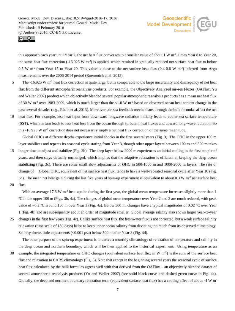
The ranges of seasonal variations of SST are realistically simulated, with the differences between the maximum and

minimum values of SST closely resembling those of OISST (Fig. 15a, b). Large seasonal variations of SST are mainly located

in the Northern Hemisphere, especially in the northwest Pacific and along the U.S. east coast. Compared to observations, the 15

modelled SST variations tend to be lower in the tropical oceans and Southern Ocean, and higher in the subtropical gyres. The

model also captures the phase of SST seasonal cycles, with Northern (Southern) Hemisphere reaching peak SST in boreal

Summer/Autumn (Winter/Spring). The complex phase patterns in the tropical Pacific are also correctly simulated in the model

(Fig. 15c, d).

The OFAM3-JRA55 run also simulates the sea level seasonal variations, consistent with 1/4° satellite altimeter observations 20

from the Archiving, Validation and Interpretation of Satellite Oceanographic data (AVISO; Ducet et al. 2000) (Fig. 16a, b).

Large seasonal variations of sea level can be mainly found in shallow marginal seas, Kuroshio Extension, Gulf Stream

Extension, and tropical regions. The Southern Ocean, south Pacific and Atlantic have very small seasonal variations (<2 cm).

The model also captures the phase of sea level seasonal cycles (Fig. 16c, d), though the phase patterns of sea level are more

complicated than those of SST, possibly because sea level variations reflect the integral of variability from the surface to the 25

ocean floor, and thus are determined by changes in the ocean interior. The amplitude and phase of the modelled sea level

seasonal cycle are very similar to reports from Vinogradov et al. (2008), based on results from the Estimating the Circulation

and Climate of the Ocean (ECCO) version 2 product over 1992-2004 (see their Fig. 3). The inter-hemisphere contrast is due

to the annual cycle of surface heating and cooling, whereas the westward propagation in the tropical oceans is related to the

annual Rossby waves. 30

4.3 ENSO-related Interannual variation

As the dominant mode of climate variability on interannual time scale, ENSO can have signatures in the ocean and atmosphere,

both inside and outside of its source region in the tropical Pacific (e.g., Alexander et al. 2002; McPhaden 2006; Roemmich


13

and Gilson 2011). Therefore, correctly representing interannual variations associated with ENSO events is another measure of

model performance. Here we examine SST and sea level evolution on interannual time scale in the tropical Pacific, since these

two variables have strong interannual variability there and their variability mechanisms have been extensively examined before

(e.g., Jin et al. 2006; Zhang and McPhaden 2006; Landerer et al., 2008; Zhang and Church 2012). We will also examine ENSO-

related variability in BGC fields. 5

4.3.1 SST and sea level anomalies

The temporal evolution of the equatorial SST and sea level anomalies averaged over 2°N-2°S from OFAM3-JRA55 run agrees

well with their respective observations, showing correct longitude-time evolution of SST and sea level that align with ENSO

events (Fig. 17). Warm (cold) SST anomalies and high (low) sea level anomalies usually appear in the central and eastern

equatorial Pacific during El Niño (La Niña) events. Starting from the beginning of the 21st century, central Pacific-type El 10

Niño events have been occurring more frequently, with maximum SST and sea level anomalies being located in the central or

central-eastern equatorial Pacific rather than eastern equatorial Pacific (e.g., Kao and Yu 2009; McPhaden et al. 2011).

We also compare major Niño SST indices with those from the OISST (Fig. 18). All major El Niño and La Niña events are

captured well, including the very strong El Niño events in 1982-83 and 1997-98, and a strong El Niño in 1987-88, and strong

La Niña events in 1988-89, 1999-2000, and 2010-11. The timing of the onset and decline of these events, the magnitudes of 15

the four indices, and their phases of the evolution, agree well between the model and observations, as indicated by high (>0.90)

correlation coefficients for all four Niño indices (correlation coefficients are shown in Fig. 18). The RMS differences between

modelled and observed Niño indices are quite small, slightly increasing from west to east (Niño-4 to Niño-1.2). Higher RMS

difference in Niño-1.2 index (0.46 oC) may be associated with warm bias in the mean SST there (Fig. 7c).

4.3.2 Biogeochemical fields 20

The largest interannual variability of PP occurs in the tropical Pacific, which is consistent with the observations (Fig. 13c, d).

This variability is mainly associated with ENSO and also produces large variability in the air-sea fluxes of CO2 (Fig. 14c). The

simulated pattern of PP interannual variability (Fig. 13c) is comparable to the estimate derived from remotely sensed ocean

colour (Fig. 13d) but the simulated magnitude is larger. The greater magnitude of variability is particularly apparent in the

Western Pacific and along the boundary of the oligotrophic gyres. Part of the difference may be related to the sub-surface 25

phytoplankton maxima that can occur in regions like the Western Pacific (LeBorgne et al. 2011). These regions contribute to

the simulated productivity but have minimal surface expression, so are not detected by remote sensing.

For the simulated interannual variability in the natural air-sea carbon fluxes the tropics are again the regions with the greatest

variability (Fig. 14c). There is also elevated variability in the Southern Ocean and North Pacific. This spatial pattern of high

variability in the Equatorial Pacific and Southern Ocean is consistent with our present interpretation of the observations (Feely 30

et al., 1999; Lenton et al., 2013), but existing data are too sparse to directly assess the simulated magnitude with observations


14

(Wanninkhof et al., 2013). However, the simulated global interannual variability (0.3 PgC yr-1) is comparable to recent

synthesis of model and observations (0.2- 0.4 PgC yr-1) (Wanninkhof et al., 2013).

Overall the OFAM3-JRA55 experiment realistically represents ENSO-related variability in productivity and carbon fluxes,

SST and sea level.

5

4.4 Non-seasonal and mesoscale variability

4.4.1 SST anomaly

The standard deviation of monthly SST anomaly (seasonal cycle removed) shows a similar pattern between the OFAM3-

JRA55 experiment and OISST (Fig. 19). Spatial correlation and RMS difference between modelled and observed fields is 0.70

and 0.15 oC, respectively. Note that the model SST demonstrates slightly lower variability around the tropics and higher 10

variability in the extra-tropical regions, especially around the major WBCs (in particular, the Gulf Stream and the Kuroshio)

and the ACC. This could be due to the fact that OFAM3 is capable of simulating higher SST variability which results from

eddy activity, since OFAM3 has an eddy-resolving resolution (1/10o), while the OISST has a coarser resolution (1/4o). In other

words, it’s possible that the 1/10o-resolution model may capture the SST variability more than the 1/4o-resolution observational

product. 15

A close inspection of the maps in Fig. 19 shows good agreement between the observed and modelled fields in many areas.

For example, the standard deviation of SST anomaly in the Kuroshio Extension region shows two zonal tongues of high

variability extending from the coast of Japan into the central Pacific. This feature is evident in both the model and observations.

Both modelled and observed SST variability display similar characteristics in the Gulf Stream extension, the Aghulas

retroflection region, and the Brazil Malvinas confluence region. In the tropics, the zonal extent of the high SST variability 20

along the equator, between about 150oE and South America, is well reproduced in the model.

The standard deviation of the SST anomaly in regions of coastal upwelling (e.g., Benguela Current, Peru Current, Canary

Current) is well reproduced in the model – with relatively high variability extending from the coast towards the interior of the

respective ocean basins. However, we note that the precise locations of these local maxima in the model are not always co-

located with the corresponding maxima in the observations. For example, the modelled maxima for the Benguela Current is 25

farther south than in the observations, and the modelled maxima in the Peru Current system does not extend into the basin

interior as pronounced as it does in the observations.

The regions where the model SST variability is less than the observations appear to be in the central South Pacific basin,

the central South Atlantic basin, and in the central South Indian basin. In those regions, either the model variability is too

quiescent, or the variability in the mapped observations is too “noisy”. We note that the signal to noise ratio in the observations 30

is small in those regions, so the relative accuracy of the SST maps are likely to be poorer than elsewhere. The model SST tends

to be constrained by the atmospheric forcing through the bulk formulas, which could be another source of errors.


15

4.4.2 Sea level anomaly

The standard deviation of monthly sea level anomaly (SLA) from the model compares well with that derived from satellite

altimeter observations from AVISO. Spatial correlation and RMS difference between model and observations is 0.85 and 0.02

m, respectively (Fig. 20). As found in previous OFAM3 run (Oke et al. 2013a), high SLA standard deviations can be found

along the ACC, in the WBCs and their extension regions (namely, Kuroshio, Gulf Stream, Agulhas Current, East Australian 5

Current and Brazil Current), where mesoscale eddy activity is prevalent (Fig. 21). The standard deviation of modelled SLA in

the tropics tends to be slightly less than in the observations, though it has the right spatial structure in the tropical Pacific, i.e.,

one peak on the equator in the east, and two peaks off the equator in the west (e.g., Zhang et al. 2012). As noted for the transport

variability, this smaller SLA standard deviation may be associated with weaker wind stress calculated through the bulk

formulas rather than directly applied wind stress available from the JRA55 reanalysis (not shown). 10

4.4.3 Eddy Kinetic Energy

The spatial distribution of the eddy kinetic energy (EKE, see appendix for definition and derivation of EKE) outside of the

equatorial region is consistent with that derived from satellite altimeter data (Pascual et al. 2006) and surface drifter data

(Lumpkin and Johnson 2013). There is good agreement of EKE distribution between modelled and observed fields for the

long-term mean (Fig. 21a, b), and spatio-temporal distribution as indicated by the monthly snapshot (Fig. 21c, d). The ACC, 15

WBCs and their extension regions have the highest EKE. Among the eastern boundary current systems, the poleward-flowing

Leeuwin Current displays the highest EKE, consistent with observations (Feng et al. 2005). The model also shows high EKE

in the equatorial region that is associated with the ocean’s response to strong coupled intraseasonal and tropical instability

waves.

20

4.5 Historical trends and changes

We have attempted to set-up the model described here for climate-change studies. In this sub-section, we examine several

fields in terms of linear trends, or changes over two 18-year periods: 1979-1996 and 1997-2014.

4.5.1 OHC

Global OHC, integrating variations of the ocean temperature from the surface to the bottom, is an important component for 25

energy budget in our climate system, since the majority (93%) of heat uptake is in the climate system is stored in the ocean

(e.g., Rhein et al. 2013).

The time series of model global OHC is within the envelope of three benchmark ocean reanalysis products: Simple Ocean

Data Assimilation (SODA, v2.2.4, Carton and Giese, 2008), German ECCO (GECCO, v2, Köhl, 2015), and ECMWF ORAS4

(Balmaseda et al. 2013), as well as the historical reconstruction for the upper 700 m only by Domingue et al. (2008, v3.1) (Fig. 30

22a). The global OHC also compares well with two Argo-based datasets (0-2000 m only) since 2006: one is based on optimal


16

interpolation (OI) by Roemmich and Gilson (2009), and the other is based on reduced space optimal interpolation (RSOI)

developed by the CSIRO sea level group (Roemmich et al. 2015). This is a good indication that the model represents change

and variability of OHC realistically, despite the fact that no observational data are assimilated in our historical experiment. We

regard such good representation as a significant achievement for a nearly free OGCM run – indicating that the careful

configuration of the model has resulted in a reliable and realistic simulation. We also note that the total OHC change over the 5

36-year historical experiment is only about half of that over 20-year spinup experiment (compare Figs. 3a and 22a), which

suggests the critical importance of proper spin-up before any meaningful simulation of OHC.

There is a clear seasonal cycle in global OHC, with maximum in austral summer and minimum in austral winter (Fig. 22a).

Additionally, climate variability in particular ENSO and natural forcing such as volcanic eruption also affect global OHC

evolution, for example the reduction of OHC associated with Mt Pinatubo volcanic eruption in 1991, consistent with Church 10

et al. (2013) and Gregory et al. (2013). Removing these variations from seasonal to interannual time scales, one can see a

gradually increase of OHC over 1979-2014. The global OHC increase, equivalently expressed in surface heat flux, has a mean

value of 0.42 W m-2 over 36 years, which is within the range of 0.4~0.6 W m-2 derived from Argo measurements in the past

decade by Roemmich et al. (2015).

The seasonal cycle is most obvious in the OHC globally integrated over the upper 100 m. Ocean heat uptake begins to 15

dominate from 200-300 m, with very similar rates in 300-400 m and 400-500 m, with a small decrease of OHC in the upper

100 m (Fig. 22b). Most of the uptake occurs in the upper 1000 m, with the upper 500 m contributing more than 500-1000 m

(Fig. 22c). OHC increase in 1000-2000 m is weak, about 2x1022 Joule over 36 years. The OHC below 2000 m decreases

slightly with its magnitude being ~9 % of total OHC gain over full depths, which indicates that non-adaptive temperature

relaxation in the deep ocean keeps the deep-ocean from drifting far from the initial conditions. 20

4.5.2 Trends of SST and sea level

Linear trends of SST and sea level over 1993-2014 from the model match those derived from observations (Figs. 23, 24). A

negative PDO-like pattern (Mantua and Hare 2002), i.e., negative trends in the eastern Pacific and positive trends in the western

Pacific, can be found in both simulated and observed SST and sea level trend maps, which should be mainly related to the

PDO’s transition from positive phase in early 1990s to negative phase in recent years (e.g., Zhang and Church, 2012; 25

Meyssignac et al. 2012; England et al. 2014). Therefore, it is challenging to identify robust SST and sea level signatures of

externally driven climate change during the last two decades, over which internal climate variability can easily dominate

(Solomon et al. 2011; Chepurin et al. 2014; Lyu et al. 2015). Warming SST trends and rising sea level trends can be found in

the south Indian Ocean, which may be partially associated the PDO phase transition, since the Indo-Pacific does experience

coherent variations associated with large-scale climate variability such as ENSO and PDO through planetary wave propagation 30

(Feng et al. 2010; Han et al. 2014).


17

4.5.3 Changes in horizontal and meridional overturning circulation

Horizontal gyre circulations and meridional overturning circulations are derived from two 18-year periods: 1979-1996 and

1997-2014, to examine decadal changes between them in the OFAM3-JRA55 experiment (Figs. 10c, d and 11d-f).

Differences of horizontal gyre circulation between two periods can be found globally, which have more regional features than

its long-term mean over 1979-2014 (Fig. 10a, c). Changes of volume transport in key straits and passages between two sub 5

periods (Table 2) are generally small (less than 2 Sv). Transport changes derived from wind stress based on the Sverdrup

Balance and Island Rule, are a good approximation for explaining changes of horizontal gyre circulation, especially in the

Indian and Pacific Ocean basins (Fig. 10d). Large changes around New Zealand are associated with the strengthening of the

subtropical gyre circulation in the South Pacific Ocean (Roemmich et al. 2007). Both the tropical and subtropical gyre

circulations appear to have strengthened in the more recent period. A more detailed examination of decadal trends of the ocean 10

boundary currents around Australia from the OFAM3-JRA55 simulation is presented in a separate study (Feng et al. 2016).

For the meridional overturning circulation, changes in the Pacific are apparent in the upper ocean (Fig. 11f), with enhanced

STCs (+2 Sv in the North Pacific, -4 Sv in the South Pacific) driven by strengthened trade winds due to the phase shift of the

PDO or Interdecadal Pacific Oscillation (IPO; Feng et al. 2010). In the Atlantic, the MOC is weakened by 1.5~2 Sv (Fig. 11e).

We note that there has been a declining trend of the strength of the Atlantic MOC in the past decade (Srokosz and Bryden 15

2015). The global MOC changes are approximately the sum of MOC changes in the Indo-Pacific and Atlantic oceans (Fig.

11d), with slightly enhanced STCs in the tropics and the Deacon Cell in the Southern Ocean (Katsumata and Masuda 2013),

and weakened MOC shown in the northern mid- and high latitudes.

4.5.4 BGC

The trends of PP are small – but there is a noticeable decline in the global value over the historical simulation (Fig. 6a). The 20

simulated decline is largely related to declines in the Southern and Northern sub-tropical zones (see Fig. 6 for the definition of

zones). For the Northern sub-tropical zone the decline appears to continue from the simulated decline in the spin-up simulation.

Hence, we cannot confidently attribute it to the changes in response to historical forcings. For the Southern sub-tropics zone,

there is no decline in the spin-up simulation, which suggests that the decline reflects the influence of the historical forcing on

PP. In the other latitude bands the historical simulation shows no clear trends in PP. 25

The historical trends in the natural air-sea CO2 flux in the various zonal bands are much weaker than in the spin-up simulation

(Fig. 6b). As the upper ocean approach equilibration with the atmosphere the trends approach zero. Given the large trends in

the spin-up simulation and the corresponding weak trends in the historical simulation, we are unable to confidently attribute

trends in the historical simulation to climate forcing. The temporal behaviour of the spin-up simulation will also hinder our

ability to attribute trends in natural air-sea CO2 in the future simulation to climate change. However, year-to-year variability 30

is much greater than trends (Fig. 14c, d), indicating that the simulation has reasonable responses in carbon flux to interannual

variability in forcing.


18

5 Discussion and Summary

In this study, we modified a near-global eddy-resolving ocean general circulation model for climate applications, especially

focusing on reducing unrealistic model drift that could contaminate the climate signals of interest. We first spin-up the model

with repeated year 1979 forcing for two decades, with temperature and salinity in the deep ocean relaxed to their observed

monthly climatological values. Then the diagnosed monthly temperature and salinity relaxation from the last five years of the 5

spin-up experiment is applied to the historical experiment (1979-2014). The model’s performance over the 36-year historical

period is compared to various observational datasets. We found the model realistically reproduces the mean states, seasonal

and interannual variations, mesoscale variability, and trends in the ocean. As an example of our model’s performance, the

modelled global OHC change over the past 36 years compares well with three ocean reanalysis products, two Argo-based

datasets and one historical reconstruction dataset. 10

Despite quite good model performance, our model experiment, by no means, does not have any caveats. For example, our

model simulation still has some biases in representing features in major WBCs and their extensions, e.g., Agulhas ring

generation and pathways, location of Brazil-Malvinas Confluence, some of which may be long-existing challenges, associated

with inefficiency in our current modelling capacity. Thus advances in model development, such as better advection scheme,

may help to improve model’s performance (e.g., Bernard et al. 2006; Backeberg et al. 2009). Detailed discussion on these 15

caveats and possible solution from further model development is beyond the scope of this paper.

The design of combing adaptive relaxation of temperature and salinity during the spin-up and non-adaptive relaxation during

historical experiment is novel, though its underlying idea has been known to the modelling community, mostly applied to air-

sea fluxes. For example, surface flux correction was once a common practice for coupled climate models (e.g., Sausen et al.

1988), e.g., helped to represent ENSO variability better (Roeckner et al. 1996), but it became less common in recent years. 20

Nonetheless, Vecchi et al. (2014) recently rejuvenated such method to correct systematic ocean biases through flux correction

and achieved better performance in tropical cyclones forecasting.

We are currently continuing to run this model to downscale future climate changes in the ocean in the 21st century by using

the same configuration as the historical run. The future run, initialized at the start of 2006 from the historical run, is driven by

merged atmospheric forcing with the high-frequency component coming from current-day JRA55 reanalysis and long-term 25

climate changes derived from the ensemble mean of 17 Coupled Model Intercomparison Project Phase 5 (CMIP5) models

(Taylor et al. 2012). Preliminary examination of model output from this future experiment indicates that our strategy to mitigate

model drift is reasonable and can be successfully applied to eddy-resolving OGCM experiments spanning several decades to

a century.

The problem of model drift in climate models is well known and makes analysing and understanding of climate variability 30

and change difficult. Despite the prevalence of this problem, no popular and satisfactory solutions to this problem have been

previously described. In this study, we describe a novel approach to reduce model drift. We show that our approach works

reasonably well: the simulated variability in the model is realistic; the simulated trends agree well with observations; and the


19

artificial drifts that usually contaminate the signals of interest are small. We recommend that the climate modelling community

can consider adopting the approach described in this study as an efficient short-term solution, at the same time also develop

more sophisticated methods to address this important problem of model drift.

Appendix:

Information about Mean Kinetic Energy (MKE) and Eddy Kinetic Energy (EKE) calculations 5

Here is the detailed procedure to calculate MKE and EKE from model zonal and meridional velocity fields (u, v):

1. derive the long-term average velocity (um, vm) from the daily velocity (u, v) from the model run;

2. MKE is defined as 0.5×(um2+vm2)

3. calculate the velocity anomalies u' = u – um, and v' = v – vm

4. Filter the velocity anomalies to get high-passed components (u'', v'') with cut-off period of 270 days. 10

5. Daily EKE is defined as 0.5×(u''2 + v''2), and monthly EKE is defined as the monthly mean of daily EKE.

Similarly, weekly altimeter sea level over 1993-2014 at 1/4o horizontal resolution from AVISO is used to derive surface

current based on geostrophic balance. Then EKE from altimeter is derived from surface current in the same manner as the

EKE from model.

15

Acknowledgements. This work is supported by the Ocean Downscaling Strategic Project, funded by CSIRO Oceans and

Atmosphere, with close collaboration with the Bluelink team (http://wp.csiro.au/bluelink/global/). All modelling experiments

have been carried out at the Australian National Computing Infrastructure (NCI, http://nci.org.au/). Merged satellite altimetry

dataset is provided by AVISO (http://www.aviso.altimetry.fr/en/home.html). Japanese 55-year Reanalysis (JRA-55) product

is provided by the Japan Meteorological Agency (http://jra.kishou.go.jp/JRA-55/index_en.html). We also wish to acknowledge 20

use of Ferret program (http://ferret.pmel.noaa.gov/Ferret/) for the most of analysis and graphics in this paper, which makes it

possible to analyze large-size datasets. We thank Melissa Bowen, Clothilde Langlais and Tatiana Rykova for critically reading

the earlier versions of the manuscript.

References

Adcroft, A., Hill, C., and Marshall, L.: Representation of topography by shaved cells in a height coordinate ocean model, Mon. 25

Weather Rev., 125, 2293–2315, 1997.

Alexander, M. A., Bladé, I., Newman, M., Lanzante, J. R., Lau, N.-C., and Scott, J. D.: The atmospheric bridge: The influence

of ENSO teleconnections on air–sea interaction over the global oceans. J. Climate, 15, 2205–2231, 2002.

Backeberg, B. C., Bertino, L., and Johannessen, J. A.: Evaluating two numerical advection schemes in HYCOM for eddy-

resolving modelling of the Agulhas Current, Ocean Sci., 5, 173-190, 2009. 30

Balmaseda, M. A., Mogensen, K., and Weaver, A. T.: Evaluation of the ECMWF ocean reanalysis system ORAS4. Q. J. R.

Meteorol. Soc. 139: 1132–1161. DOI:10.1002/qj.2063, 2013.


20

Barnier, B., Madec, G., Penduff, T., Molines, J., Treguier, A., Sommer, J. L., Beckmann, A., Biastoch, A., Böning, C., Dengg,

J., Derval, C., Durand, E., Gulev, S., Remy, E., Talandier, C., Theetten, S., Maltrud, M., McClean, J., and Cuevas, B. D.:

Impact of partial steps and momentum advection schemes in a global ocean circulation model at eddy permitting resolution,

Ocean Dyn., 56, 543–567, 2006.

Behrenfeld, M. J. and Falkowski, P. G.: Photosynthetic rates derived from satellite-based chlorophyll concentration, 5

Limnology and Oceanography, 42, 1-20, 1997.

Carton, J. A. and Giese, B. S.: A Reanalysis of Ocean Climate Using Simple Ocean Data Assimilation (SODA). Mon. Wea.

Rev., 136, 2999–3017. doi: http://dx.doi.org/10.1175/2007MWR1978.1, 2008.

Chassignet, E. P., Hurlburt, H. E., Smedstad, O. M., Halliwell, G. R., Hogan, P. J., Wallcraft, A. J., Baraille, R., and Bleck,

R.: The HYCOM (HYbrid Coordinate Ocean Model) data assimilative system, J. Mar. Syst., 65 (2007), pp. 60–83, 2007. 10

Chelton, D. B., deSzoeke, R. A., Schlax, M. G., El Naggar, K. and Siwertz, N.: Geographical variability of the first-baroclinic

Rossby radius of deformation. J. Phys. Oceanogr., 28, 433-460, 1998.

Chen, D., Rothstein, L., and Busalacchi, A.: A hybrid vertical mixing scheme and its application to tropical ocean models, J.

Phys. Oceanogr., 24, 2156–2179, 1994.

Chepurin, G. A., Carton, J. A., and Leuliette, E.: Sea level in ocean reanalyses and tide gauges, J. Geophys. Res. Oceans, 119, 15

147–155, doi:10.1002/2013JC009365, 2014.

Church, J. A., Monselesan, D., Gregory, J. M., and Marzeion, B.: Evaluating the ability of process based models to project

sea-level change, Environ. Res. Lett. 8, 014051, doi:10.1088/1748-9326/8/1/014051, 2013.

Dai, A. and Trenberth, K. E.: Estimates of freshwater discharge from continents: Latitudinal and seasonal variations, J.

Hydrometeor., 3, 660–687, 2002. 20

Dai, A., Qian, T., Trenberth, K. E., and Milliman, J. D.: Changes in continental freshwater discharge from 1948–2004, J.

Climate, 22, 2773–2791, 2009.

de Miranda, A. P., Barnier, B., and Dewa, W.: On the dynamics of the Zapiola Anticyclone, J. Geophys. Res., 104, 21,137–

21,149, 1999.

Domingues, C. M., Church, J. A., White, N. J., Gleckler, P. J., Wijffels, S. E., Barker, P. M., and Dunn, J. R.: Improved 25

estimates of upper-ocean warming and multi-decadal sea-level rise, Nature, 453, 1090–1094, doi:10.1038/nature07080,

2008.

Ducet, N., Le Traon, P. Y., and Reverdin, G.: Global high-resolution mapping of ocean circulation from TOPEX/POSEIDON

and ERS-1 and-2, J. Geophys. Res., 105, 19477–19498, 2000.

England, M. H., et al.: Recent intensification of wind-driven circulation in the Pacific and the ongoing warming hiatus, Nat. 30

Clim. Change, 4, 222–227, doi:10.1038/nclimate2106, 2014.

Eppley, R. W.: Temperature and phytoplankton growth in the sea, Fishery Bulletin, 70, 1063-1085, 1972.

Feely, R. A., Wanninkhof, R., Takahashi, T., and Tans, P.: Influence of El Niño on the equatorial Pacific contribution to

atmospheric CO2 accumulation, Nature, 398, 597–601, 1999.


21

Feng, M., Wijffels, S. E., Godfrey, S. and Meyers, G.: Do Eddies Play a Role in the Momentum Balance of the Leeuwin

Current?. J. Phys. Oceanogr., 35, 964–975. doi: http://dx.doi.org/10.1175/JPO2730.1, 2005.

Feng, M., McPhaden, M. J., and Lee, T.: Decadal variability of the Pacific subtropical cells and their influence on the southeast

Indian Ocean, Geophys. Res. Lett., 37, L09606, doi:10.1029/2010GL042796, 2010.

Feng, M., Schiller, A., Zhang, X., Oke, P., Monselesan, D., Chamberlain, M., and Matear, R.: Energizing ocean boundary 5

current systems around Australia over the past 36 years – as simulated in a near-global eddy-resolving ocean model,

submitted to J. Geophys. Res., 2016.

Ferrari, F. and Wunch, C.: Ocean circulation kinetic energy: reservoirs, sources, and sinks. Annu. Rev. Fluid Mech, 41, 253–

82, 2009.

Garcia, H., Locarnini, R., and Boyer, T.: World Ocean Atlas 2005, Volume 3: Dissolved Oxygen, Apparent Oxygen 10

Utilization,, in: NOAA Atlas NESDIS 63, edited by Levitus, S., p. 342, US Gov. Print. Off., U.S. Government Printing

Office, Washington, D.C., 2006a.

Garcia, H., Locarnini, R., Boyer, T., and Antonov, J.: World Ocean Atlas 2005, Volume 4: Nutrients (phosphate, nitrate,

silicate), in: NOAA Atlas NESDIS 63, edited by Levitus, S., p. 396, US Gov. Print. Off., U.S. Government Printing Office,

Washington, D.C., 2006b. 15

Gill, A. E.: Atmosphere-Ocean Dynamics. London and New York: Academic Press, 1982.

Godfrey, J. S.: A Sverdrup model of the depth-integrated flow for the world ocean allowing for island circulations. Geophys.

Astrophys. Fluid Dyn., 45, 89-112, 1989.

Gregory, J. M., White, N. J., Church, J. A., Bierkens, M. F. P., Box, J. E., van den Broeke, M. R., Cogley, J. G., Fettweis, X.,

Hanna, E., Huybrechts, P., Konikow, L. F., Leclercq, P. W., Marzeion, B., Oerlemans, J., Tamisiea, M. E., Wada, Y., 20

Wake, L. M., and van de Wal, R. S. W.: Twentieth-Century Global-Mean Sea Level Rise: Is the Whole Greater than the

Sum of the Parts?. J. Climate, 26, 4476–4499. doi: http://dx.doi.org/10.1175/JCLI-D-12-00319.1, 2013.

Griffies, S. M.: Elements of MOM4p1, GFDL Ocean Group Technical Report 6, Tech. rep., NOAA/Geophysical Fluid

Dynamics Laboratory, 2009.

Griffies, S. M. and Hallberg, R. W.: Biharmonic friction with a Smagorinsky-like viscosity for use in large-scale eddy 25

permitting ocean models, Mon. Weather Rev., 128, 2935–2946, 2000.

Griffies, S. M., Boning, C., Bryan, F. O., Chassignet, E. P., Gerdes, R., Hasumi, H., Hirst, A., Treguier, A.-M., and Webb, D.:

Development in ocean climate modeling. Ocean Model. 2, 123–192, 2000.

Griffies, S. M., et al.: and Co-authors: Coordinated Ocean-ice Reference Experiments (COREs). Ocean Modelling, 26, 1–46,

2009. 30

Griffies, S. M., et al.: An assessment of global and regional sea level for years 1993–2007 in a suite of interannual CORE-II

simulations, Ocean Modelling, 78, 35-89. Doi: http://dx.doi.org/10.1016/j.ocemod.2014.03.004, 2014.

Griffies, S. M., et al.: Impacts on ocean heat from transient mesoscale eddies in a hierarchy of climate models. J. Climate, 28,

952–977, 2015.


22

Han, W., Vialard, J., McPhaden, M. J., Lee, T., Masumoto, Y., Feng, M., and de Ruijter, W. P. M.: Indian Ocean Decadal

Variability: A Review. Bull. Amer. Meteor. Soc., 95, 1679–1703. doi: http://dx.doi.org/10.1175/BAMS-D-13-00028.1,

2014.

Hautala, S. L., Roemmich, D., and Schmitz, W. J.: Is the North Pacific in Sverdrup balance along 24oN? J. Geophys. Res., 99,

16041–16052, 1994. 5

Hopps, W., Palmer, M. and Monselesan, D.: An Energy Conservation Analysis of Ocean Drift in the CMIP5 Global Coupled

Models, J. Climate, doi:10.1175/JCLI-D-15-0477.1, 2016.

Jin, F.-F., Kim, S. T., and Bejarano, L.: A coupled-stability index for ENSO, Geophys. Res. Lett., 33, L23708,

doi:10.1029/2006GL027221, 2006.

Johns, W. E., Baringer, M. O., Beal, L. M., Cunningham, S. A., Kanzow, T., Bryden, H. L., Hirschi, J. J. M., Marotzke, J., 10

Meinen, C. S., Shaw, B., and Curry, R.: Continuous, Array-Based Estimates of Atlantic Ocean Heat Transport at 26.5°N.

J. Climate, 24, 2429–2449. doi: http://dx.doi.org/10.1175/2010JCLI3997.1, 2011.

Johnson, G. C., Sloyan. B. M., Kessler, W. S., and McTaggart, K. E.: Direct measurements of upper ocean currents and water

properties across the tropical Pacific Ocean during the 1990's. Prog. Oceanogr., 52, 31–61, 2002.

IPCC, 2013: Climate Change: The Physical Science Basis. Contribution of Working Group I to the Fifth Assessment Report 15

of the Intergovernmental Panel on Climate Change [Stocker, T.F., Qin, D., Plattner, G.-K., Tignor, M., Allen, S. K.,

Boschung, J., Nauels, A., Xia, Y., Bex, V. and Midgley, P. M. (eds.)]. Cambridge University Press, Cambridge, United

Kingdom and New York, NY, USA, 1535 pp, doi:10.1017/CBO9781107415324, 2013.

Kao, H.-Y. and Yu, J.-Y.: Contrasting Eastern-Pacific and Central-Pacific Types of ENSO. J. Climate, 22, 615–632. doi:

http://dx.doi.org/10.1175/2008JCLI2309.1, 2009. 20

Katsumata, K. and Masuda, S.: Variability in Southern Hemisphere Ocean Circulation from the 1980s to the 2000s. J. Phys.

Oceanogr., 43, 1981–2007. doi: http://dx.doi.org/10.1175/JPO-D-12-0209.1, 2013.

Key, R. M., Kozyr, A., Sabine, C. L., Lee, K., Wanninkhof, R., Bullister, J. L., Feely, R. A., Millero, F. J., Mordy, C., and

Peng, T. H.: A global ocean carbon climatology: Results from Global Data Analysis Project (GLODAP), Global

Biogeochemical Cycles, 18, GB4031, 2004. 25

Klinger, B. A. and Marotzke, J.: Meridional heat transport by the subtropical cell. J. Phys. Oceanogr., 30, 696– 705, 2000.

Kobayashi, S., Ota, Y., Harada, Y., Ebita, A., Moriya, M., Onoda, H., Onogi, K., Kamahori, H., Kobayashi, C., Endo, H.,

Miyaoka, K., and Takahashi, K.: The JRA-55 Reanalysis: General Specifications and Basic Characteristics. J. Meteor. Soc.

Japan, 93, 5-48, doi:10.2151/jmsj.2015-001, 2015.

Köhl, A.: Evaluation of the GECCO2 Ocean Synthesis: Transports of Volume, Heat and Freshwater in the Atlantic, Q. J. R. 30

Met. Soc., 141(686), 166-181, doi: 10.1002/qj.2347, 2015.

Landerer, F. W., Jungclaus, J. H. and Marotzke, J.: El Niño–Southern Oscillation signals in sea level, surface mass

redistribution, and degree two geoid coefficients, J. Geophys. Res., 113, C08014, doi:10.1029/2008JC004767, 2008.


23

Large, W. G. and Yeager, S. G.: Diurnal to decadal global forcing for ocean and sea-ice models: the data sets and flux

climatologies, NCAR Technical Note, TN-460, Boulder Colorado, USA, 2004.

Large W. G., McWilliams, J. C., and Doney, S. C.: Oceanic vertical mixing: A review and a model with a non-local boundary

layer parametrization. Rev. Geophys., 32, 363-403, 1994.

Law, R. M., Ziehn, T., Matear, R. J., Lenton, A., Chamberlain, M. A., Stevens, L., Wang, Y.-P., Bi, D., and Yan, H.: The 5

carbon cycle in the Australian Climate and Earth System Simulator (ACCESS-ESM1). 1. Model description and pre-

industrial simulation. Geosci. Model Dev. Discussion, 8, 8063-8116, doi:10.5194/gmdd-8-8063-2015, 2015.

Lee, H.-C., Rosati, A., and Spelman, M.: Barotropic tidal mixing effects in a coupled climate model: ocean conditions in the

northern Atlantic, Ocean Model., 11, 464–470, 2006.

Lenton, A., et al.: Sea–air CO2 fluxes in the Southern Ocean for the period 1990-2009. Biogeosciences, 10, 4037–4054, 2013. 10

Lumpkin, R. and Johnson, G. C.: Global ocean surface velocities from drifters: Mean, variance, El Niño–Southern Oscillation

response, and seasonal cycle, J. Geophys. Res. Oceans, 118, 2992–3006, doi:10.1002/jgrc.20210, 2013.

Lyu, K., Zhang, X., Church, J. A., and Hu, J.: Quantifying internally-generated and externally-forced climate signals at regional

scales in CMIP5 models, Geophys. Res. Lett., 42, Doi:10.1002/2015GL065508, 2015.

Maltrud, M. E. and McClean, J. L.: An eddy resolving global 1/10o ocean simulation. Ocean modelling, 8, 31-54. 15

Doi:10.1016/j.ocemod.2003.12.001, 2005.

Mantua, N. J. and Hare, S. R.: The Pacific Decadal Oscillation, J. Oceanogr., 58, 35–44, doi:10.1023/A:1015820616384, 2002.

Masumoto, Y., Sasaki, H., Kagimoto, T., Komori, N., Ishida, A., Sasai, Y., Miyama, T., Motoi, T., Mitsudera, H., Takahashi,

K, Sakuma, H., and Yamagata, T.: A fifty-year eddy-resolving simulation of the world ocean—Preliminary outcomes of

OFES (OGCM for the Earth Simulator). J. Earth Simulator, 1, 35–56, 2004. 20

Matear, R. J., Chamberlain, M. A., Sun, C. and Feng, M.: Climate change projection of the Tasman Sea from and eddy-

resolving ocean model. J. Geophys. Res. Oceans, 118, 2961-2976. doi:10.1002/jgrc.20202, 2013.

Maximenko, N., Niiler, P., Centurioni, L., Rio, M.-H., Melnichenko, O., Chambers, D., Zlotnicki, V., and Galperin, B.: Mean

Dynamic Topography of the Ocean Derived from Satellite and Drifting Buoy Data Using Three Different Techniques. J.

Atmos. Oceanic Technol., 26, 1910–1919, 2009. 25

McClean, J. L., Poulain, P.-M., Pelton, J. W., and Maltrud, M. E.: Eulerian and Lagrangian Statistics from Surface Drifters

and a High-Resolution POP Simulation in the North Atlantic. J. Phys. Oceanogr., 32, 2472–2491, 2002.

McGillicuddy, D. J., Jr., Robinson, A. R., Siegel, D. A., Jannasch, H. W., Johnson, R., Dickey, T. D., McNeil, J., Michaels,

A. F. and Knap, A. H., Influence of mesoscale eddies on new production in the Sargasso Sea, Nature, 394, 263 – 265, 1998.

McPhaden, M. J. and Zhang, D.: Slowdown of the meridional overturning circulation in the upper Pacific Ocean, Nature, 415, 30

603-608. doi:10.1038/415603a, 2002.

McPhaden, M. J., Zebiak, S. E., and Glantz, M. H.: ENSO as an integrating concept in Earth science, Science, 314, 1740–

1745, doi:10.1126/science.1132588, 2006.

McWilliams, J. C.: Modeling the oceanic general circulation, Annu. Rev. Fluid. Mech., 28, 215-248, 1996.


24

Meyssignac, B., Salas y Melia, D., Becker, M., Llovel, W., and Cazenave, A.: Tropical Pacific spatial trend patterns in observed

sea level: internal variability and/or anthropogenic signature?, Clim. Past, 8, 349–389, doi:10.5194/cpd-8-349-2012, 2012.

NASA Goddard Space Flight Center, Ocean Ecology Laboratory, Ocean Biology Processing Group, SeaWiFS Ocean Color

Data. doi:10.5067/ORBVIEW-2/SEAWIFS_OC.2014.0, 2014.

Oke, P. R., Schiller, A., Griffin, D. A., and Brassington, G. B.: Ensemble data assimilation for an eddy-resolving ocean model 5

of the Australian Region, Q. J. R. Meteorol. Soc., 131, 3301– 3311, 2005.

Oke, P. R, Griffin, D. A., Schiller, A., Matear, R. J., Fiedler, R., Mansbridge, J., Lenton, A., Cahill, M., Chamberlain, M. A.,

and Ridgway, K.: Evaluation of a near-global eddy-resolving ocean model, Geosci. Model Dev., 6, 591–615.

doi:10.5194/gmd-6-591-2013, 2013a.

Oke, P. R., Sakov, V., Cahill, M. L., Dunn, J. R., Fiedler, R., Griffin, D. A., Mansbridge, J. V., Ridgway, K. R., and Schiller, 10

A.: Towards a dynamically balanced eddy-resolving ocean reanalysis: BRAN3, Ocean Modelling, 67, 52-

70,10.1016/j.ocemod.2013.03.008, 2013b.

Oschlies, A. and Schartau, M.: Basin-scale performance of a locally optimized marine ecosystem model, J. Marine Research,

63, 335-358, 2005.

Pascual, A., Fauge`re, Y., Larnicol, G., and Le Traon, P.-Y.: Improved description of the ocean mesoscale variability by 15

combining four satellite altimeters, Geophys. Res. Lett., 33, L02611, doi:10.1029/2005GL024633, 2006.

Reynolds, R. W., Smith, T. M., Liu, C., Chelton, D. B., Casey, K. S., and Schlax, M. G.: Daily high-resolution-blended analyses

for sea surface temperature. J. Climate, 20, 5473–5496, doi:10.1175/2007JCLI1824.1, 2007.

Rhein, M., Rintoul, S. R., Aoki, S., Campos, E., Chambers, D., Feely, R. A., Gulev, S., Johnson, G. C., Josey, S. A., Kostianoy,

A., Mauritzen, C., Roemmich, D., Talley, L. D., and Wang, F.: Observations: Ocean. In: Climate Change 2013: The 20

Physical Science Basis. Contribution of Working Group I to the Fifth Assessment Report of the Intergovernmental Panel

on Climate Change [Stocker, T.F., D. Qin, G.-K. Plattner, M. Tignor, S.K. Allen, J. Boschung, A. Nauels, Y. Xia, V. Bex

and P.M. Midgley (eds.)]. Cambridge University Press, Cambridge, United Kingdom and New York, NY, USA, 2013.

Ridgway, K. R. and Dunn, J. R.: Mesoscale structure of the mean East Australian Current System and its relationship with

topography, Progress Oceanogr., 56, 189–222, 2003. 25

Roeckner, E., Oberhuber, J. M., Bacher, A., Christoph, M., and Kirchner, I.: ENSO variability and atmospheric response in a

global coupled atmosphere-ocean GCM, Clim. Dyn., 12, 737-754, 1996.

Roemmich, D. and Gilson, J.: The 2004–2008 mean and annual cycle of temperature, salinity, and steric height in the global

ocean from the Argo Program, Progress in Oceanography, 82, 81-100, 2009.

Roemmich, D. and Gilson, J.: The global ocean imprint of ENSO, Geophys. Res. Lett., 38, L13606, 30

doi:10.1029/2011GL047992, 2011.

Roemmich, D. and Owens, W. B.: The Argo Project: global ocean observations for the understanding and prediction of climate

variability, Oceanography, 13(2), 45-50, 2000.


25

Roemmich, D., Gilson, J., Davis, R., Sutton, P., Wijffels, S., and Riser, S.: Decadal Spinup of the South Pacific Subtropical

Gyre. J Phys. Oceanogr., 37, 162–173, 2007.

Roemmich, D., Church, J., Gilson, J., Monselesan, D., Sutton, P., and Wijffels, S.: Unabated planetary warming and its ocean

structure since 2006, Nature Climate Change 5, 240-245, doi:10.1038/nclimate2513, 2015.

Sabine, C. L., Feely, R. A., Gruber, N., Key, R. M., Lee, K., Bullister, J. L., Wanninkhof, R., Wong, C. S., Wallace, D. W. 5

R., Tilbrook, B., Peng, T.-H., Kozyr, A., Ono, T., and Rios, A. F.: The oceanic sink for anthropogenic CO2, Science, 305,

367–371, 2004.

Sarmiento, J. L., et al.: Response of ocean ecosystems to climate warming, Global Biogeochem. Cycles, 18, GB3003,

doi:10.1029/2003GB002134, 2004.

Sasaki, H., Nonaka, M., Masumoto, Y., Sasai, Y., Uehara, H., and Sakuma, H.: An eddy-resolving hindcast simulation of the 10

quasiglobal ocean from 1950 to 2003 on the Earth Simulator. In High Resolution Numerical Modelling of the Atmosphere

and Ocean, Hamilton, K. and Ohfuchi W. (eds.), chapter 10, pp. 157–185, Springer, New York, 2008.

Sausen, R., Barthel, K., and Hasselmann, K.: Coupled ocean-atmosphere models with flux correction, Clim. Dyn., 2, 145-163,

1988.

Schiller, A., Oke, P. R., Brassington, G., Entel, M., Fiedler, R., Griffin, D. A., and Mansbridge, J. V.: Eddy-resolving ocean 15

circulation in the Asian–Australian region inferred from an ocean reanalysis effort, Progress in Oceanography, 76, 334-

365, 2008.

Schott, F., Dengler, M., and Schoenefeldt, R.: The shallow thermohaline circulation of the Indian Ocean, Prog. Oceanogr., 53,

57–103, 2002.

Sen Gupta, A., Muir, L. C., Brown, J. N., Phipps, S. J., Durack, P. J., Monselesan, D., and Sijffels, S. E.: Climate Drift in the 20

CMIP3 Models. J. Climate, 25, 4621–4640. doi: http://dx.doi.org/10.1175/JCLI-D-11-00312.1, 2012.

Sen Gupta, A., Jourdain, N. C., Brown, J. N., and Monselesan, D.: Climate Drift in the CMIP5 Models. J. Climate, 25, 8597-

8615. doi: http://dx.doi.org/10.1175/JCLI-D-12-00521.1, 2013.

Sérazin, G., Penduff, T., Grégorio, S., Barnier, B., Molines, J.-M., and Terray, L.: Intrinsic Variability of Sea Level from

Global Ocean Simulations: Spatiotemporal Scales. J. Climate, 28, 4279–4292. doi: http://dx.doi.org/10.1175/JCLI-D-14-25

00554.1, 2015.

Smith, R. D., Maltrud, M. E., Bryan, F. O., and Hecht, M. W.: Numerical Simulation of the North Atlantic Ocean at 1/10°. J.

Phys. Oceanogr., 30, 1532–1561, 2000.

Solomon, A., Goddard, L., Kumar, A., Carton, J., Deser, C., Fukumori, I., Greene, A. M., Hegerl, G., Kirtman, B., Kushnir,

Y., Newman, M., Smith, D., Vimont, D., Delworth, T., Meehl, G. A., and Stockdale, T.,: Distinguishing the Roles of 30

Natural and Anthropogenically Forced Decadal Climate Variability, Bull. Amer. Meteor. Soc., 92, 141–156, 2011

Srokosz, M. A. and Bryden, H. L.: Observing the Atlantic Meridional Overturning Circulation yields a decade of inevitable

surprises. Science, 348, 1255575. DOI: 10.1126/science.aac9225, 2015.


26

Sverdrup H. U.: Wind-driven currents in a baroclinic ocean: with application to the equatorial currents in the eastern Pacific.

Proc. Nat. Acad. Sci., 33, 318–326, 1947.

Takahashi, T., Sutherland, S.C., Wanninkhof, R., Sweeney, C., Feely, R. A., Chipman, D. W., Hales, B., Friederich, G.,

Chavez, F., Watson, A., Bakker, D. C. E., Schuster, U., Metzl, N., Yoshikawa-Inoue, H., Ishii, M., Midorikawa, T., Nojiri,

Y., Sabine, C., Olafsson, J., Arnarson, T. S., Tilbrook, B., Johannessen, T., Olsen, A., Bellerby, R., Körtzinger, A., 5

Steinhoff, T., Hoppema, M., de Baar, H. J. W., Wong, C. S., Delille, B., and Bates, N. R.: Climatological mean and decadal

changes in surface ocean pCO2, and net sea-air CO2 flux over the global oceans, Deep-Sea Research II, 56, 554–577, 2009

Taylor, K. E., Stouffer, R. J., and Meehl, G. A.: An overview of CMIP5 and the experiment design. Bull. Am. Meteorol. Soc.

93: 485–498, doi: 10.1175/BAMS-D-11-00094.1, 2012.

Tsuchiya, M.: Subsurface countercurrents in the eastern equatorial Pacific ocean. J. Mar. Res., 33, 145-175, 1975. 10

Vecchi, G. A., Delworth, T., Gudgel, R., Kapnick, S., Rosati, A., Wittenberg, A. T., Zeng, F., Anderson, W., Balaji, V., Dixon,

K., Jia, L., Kim, H.-S., Krishnamurthy, L., Msadek, R., Stern, W. F., Underwood, S. D., Villarini, G., Yang, X., and Zhang,

S.: On the Seasonal Forecasting of Regional Tropical Cyclone Activity. J. Climate, 27, 7994–8016, 2014.

Vinogradov, S. V., Ponte, R. M., Heimbach, P., and Wunsch, C.: The mean seasonal cycle in sea level estimated from a data-

constrained general circulation model, J. Geophys. Res., 113, C03032, doi:10.1029/2007JC004496, 2008. 15

Wanninkhof, R., Park, G. H., Takahashi, T., Sweeney, C., Feely, R., Nojiri, Y., Gruber, N., Doney, S. C., McKinley, G. A.,

Lenton, A., Le Quéré. C., Heinze, C., Schwinger, J., Graven, H., and Khatiwala, S.: Global ocean carbon uptake: magnitude,

variability and trends, Biogeosciences, 10, 1983–2000, 2013.

Wunch, C.: The decadal mean ocean circulation and Sverdrup balance, Journal of Marine Research, 69, 417-434, 2011.

Yu, Y., Liu, H., and Lin, P.: A quasi-global 1/10 eddy-resolving ocean general circulation model and its preliminary results. 20

Chin. Sci. Bull., doi:10.1007/s11434-012-5234-8, 2012.

Yu, L. and Weller, R. A.: Objectively Analyzed air-sea heat Fluxes for the global oce-free oceans (1981–2005). Bull. Ameri.

Meteor. Soc., 88, 527–539, 2007

Zhang, X. and Church, J. A.: Sea level trends, interannual and decadal variability in the Pacific Ocean, Geophys. Res. Lett.,

39, L21701, doi:10.1029/2012GL053240, 2012. 25

Zhang, X. and McPhaden, M. J.: Wind stress variations and interannual sea surface temperature anomalies in the eastern

equatorial Pacific. J. Climate, 19, 226–241, 2006.

Zhang, X., Cornuelle, B., and Roemmich, D.: Sensitivity of Western Boundary Transport at the Mean North Equatorial Current

Bifurcation Latitude to Wind Forcing, J. Phys. Oceanogr., 42, 2056–2072, 2012.

30


27

Table 1. Heat flux correction and annul mean net heat flux during the OFAM3-JRA55-spinup experiment.

5

10

15

20

25

30

35

Model

Year

Heat flux

correction

(W/m2)

Net mean heat

flux

(W/m2)

1 0.0 17.8

2 0.0 7.731

3 -7.731 3.122

4 -10.853 2.481

5 -13.334 1.794

6 -15.128 1.394

7 -16.925 0.842

8 -16.925 1.048

9 -16.925 0.927

10 -16.925 0.789

11 -16.925 0.715

12 -16.925 0.659

13 -16.925 0.576

14 -16.925 0.580

15 -16.925 0.480

16 -16.925 0.409

17 -16.925 0.398

18 -16.925 0.398

19 -16.925 0.364

20 -16.925 0.431


28

Table 2. Mean volume transports (Sverdrup) in key straits and passages from previous OFAM3 run (Oke et al., 2013a) over

1993-2012 and the OFAM3-JRA55 run over 1979-2014. The standard deviations are derived from monthly mean transport

values. Transport sections can be found in Fig. 1.

5

10

Straits and Passages

OFAM3

(Oke et al.

2013)

1993-2012

OFAM3-JRA55

1979-2014 1979-1996 1997-2014 1997-2014

minus

1979-1996

1 ACC Drake

Passage

151.9 ± 7.5 148.7 ± 2.9 148.4 ± 3.1 149.0 ± 2.7 0.5

2 ACC South

Africa

152.6 ± 8.1 149.6 ± 2.9 149.4 ± 3.1 149.8 ± 3.5 0.4

3 ACC Tasmania 167.8 ± 8.3 164.2 ± 3.6 163.7 ± 3.6 164.8 ± 3.5 1.1

4 Mozambique

Channel

-19.1 ± 8.0 -19.2 ± 3.9 -19.1 ± 3.8 -19.2 ± 4.1 -0.1

5 Agulhas -67.1 ± 16.5 -55.3 ± 8.1 -55.0 ± 7.8 -55.5 ± 8.3 -0.5

6 Agulhas return 5.3 ± 33.1 14.1 ± 20.4 13.9 ± 20.2 14.4 ± 20.6 0.5

7 Tasman

Leakage East

9.5 ± 6.5 12.3 ± 3.5 12.2 ± 3.4 12.3 ± 3.6 0.1

8 Tasman

Leakage West

13.9 ± 8.1 8.1 ± 5.1 8.0 ± 4.3 8.2 ± 5.9 0.1

9 East Australian

current

-17.6 ± 15.2 -15.3 ± 7.7 -15.6 ± 8.2 -14.9 ± 7.2 0.7

10 ITF Timor

Passage

-7.6 ± 1.7 -7.3 ± 1.0 -7.1 ± 0.9 -7.5 ± 0.9 -0.4

11 ITF Lombok

Strait

-1.9 ± 1.4 -1.8 ± 0.8 -1.8 ± 0.7 -1.9 ± 0.8 -0.1

12 ITF Sape Strait -0.6 ± 0.7 -0.6 ± 0.4 -0.5 ± 0.4 -0.6 ± 0.5 -0.1

13 ITF Ombai

Strait

-3.4 ± 1.9 -4.0 ± 0.8 -3.9 ± 0.8 -4.0 ± 0.9 -0.1

14 Florida current 23.8 ± 2.2 21.7 ± 1.7 22.3 ± 1.5 21.0 ± 1.5 -1.4


29

Figure 1. Model domain with blue shading indicating valid ocean grids. Horizontal transport sections are also plotted with

numerical labels corresponding to Table 2. 5


30

Figure 2. Volume-averaged kinetic energy (cm2 s-2) during the spin-up experiment as a function of model time in (a) full

depth, (b) surface model layer and (c) bottom model layer only.

5


31

Figure 3. Ocean heat content change (1023 Joule) during the spin-up experiment as a function of model time in (a) full depth,

(b) different depth ranges in the upper 500 m, and (c) different depth ranges in 500-5500 m. (d) Equivalent surface heat flux

(wm-2), showing different averages (daily, monthly and yearly).

5


32

Figure 4. Vertical profile of global average changes of (a, b) temperature and (c, d) salinity over a single model year during

the spin-up experiment. Only changes over odd model years are shown. Note different scales for left and right panels, with

much smaller scales in right panels to show details in the deep ocean. 5

10


33

Figure 5. (a) The rate of global ocean heat content change ( equivalent surface heat flux in W m-2, red curve) can be explained

by the sum of surface heat flux (black curve) and relaxation to CARS climatology (equivalent surface heat flux, blue curve), 5

during the spin-up experiment. All above curves are monthly averages. The monthly climatology of net surface heat flux from

the OAFlux (green dashed curve) is plotted over the last several years as a reference. (b) The relaxation contribution term (blue

curve) and its yearly average (cyan curve) are replotted to show more details.

10


34

Figure 6. Time series of primary productivity (top) and air-sea flux of CO2 (bottom) in the years when BGC was simulated in

the spin-up (left) and historical (right) experiments. Seasonal cycles are removed with a 12-month running-mean filter. The

latitude bands are: south oceans (SO) < 40oS; south sub-tropical (SSubT) 40oS to 10oS; Tropics 10oS to 10oN; south sub-5

tropical (NSubT) 10oN to 40oN; north oceans (NO) > 40oN.

10


35

Figure 7. Mean sea surface temperature (oC) from (a) the historical experiment and (b) NOAA 1/4° Optimum Interpolation

Sea Surface Temperature (OISST) product, and (c) differences between them. 5


36

Figure 8. Mean sea level (m) from (a) the historical experiment and (b) observation-based product (Maximenko et al. 2009),

and (c) differences between them.


37

Figure 9. (a) Mean Kinetic Energy (MKE) in the surface model layer derived from the historical experiment. MKE is 5

calculated from long-term mean of ocean current over 1979-2014. (b) MKE based on 1/2° near-surface current observations

from the satellite-tracked drifters of the Global Drifter Program.


38

Figure 10. Mean stream function (Sv =106 m3 s-1) over 1979-2014: (a) directly calculated from mean current field during the 5

historical experiment, and (b) derived from the wind stress based on the Sverdrup Balance and the Island Rule. (c) and (d),

same as (a) and (b), but show stream function differences between 1979-1996 and 1997-2014.

10

15


39

Figure 11. Mean zonally averaged meridional overturning circulation (Sv =106 m3 s-1) for the (a) entire globe, (b) Atlantic 5

basin and (c) Indo-Pacific basin. (d-f), same as (a-c), but show meridional overturning circulation differences between 1979-

1996 and 1997-2014.

10


40

5

Figure 12. Mean zonal velocity (cm s-1) on the equator (a) from the historical experiment (b) observation based on Johnson et

al. (2002). (c) and (d), same as (a) and (b), but along 140oW section.

10

15


41

5

Figure 13. Mean primary productivity from (a) the historical experiment with BGC and (b) observations, and interannual

variability as standard deviation in annual averages from (c) the historical experiment and (d) observations.

10


42

5

Figure 14. Mean air-sea flux of CO2 from (a) the historical experiment and (b) observations. (c) Interannual variability as

standard deviation in annual averages and (d) trend in the air-sea flux of CO2 from the historical experiment.

10


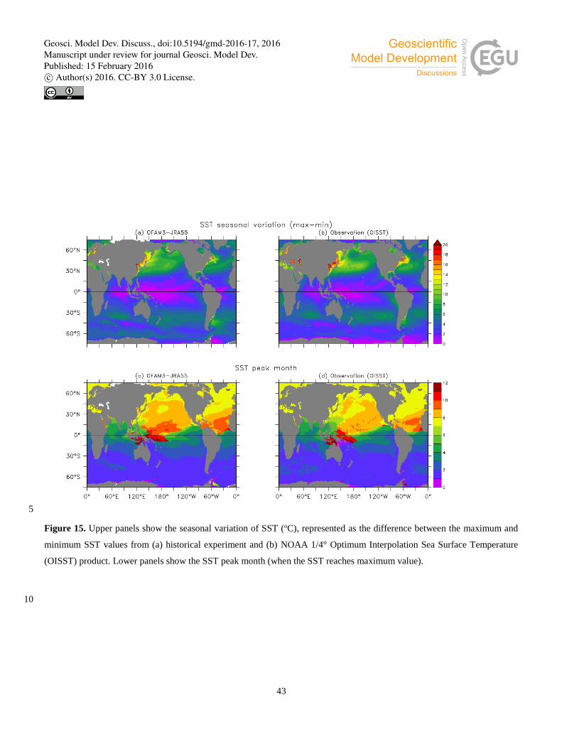
43

5

Figure 15. Upper panels show the seasonal variation of SST (oC), represented as the difference between the maximum and

minimum SST values from (a) historical experiment and (b) NOAA 1/4° Optimum Interpolation Sea Surface Temperature

(OISST) product. Lower panels show the SST peak month (when the SST reaches maximum value).

10


44

5

Figure 16. Upper panels show the seasonal variation of sea level (m), represented as the difference between the maximum and

minimum sea level values from (a) historical experiment and (b) AVISO 1/4° altimeter product. Lower panels show the sea

level peak month (when the sea level reaches maximum value).

10


45

5

Figure 17. Time–longitude diagram of interannual anomalies along the equator for sea surface temperature (oC) from (a) the

historical experiment and (b) NOAA 1/4° Optimum Interpolation Sea Surface Temperature (OISST) product, and for sea level

(m) from (c) the historical experiment and (d) AVISO 1/4° altimeter product. All data have been smoothed with a 5-month 10

running-mean filter to focus on interannual variations.

15


46

Figure 18. Comparison of Niño anomalies (oC) between the historical experiment and observation (NOAA OISST) for (a)

Niño-1.2 (90-80oW, 10-0oS), (b) Niño-3 (150-90oW, 5oS -5oN), (c) Niño-3.4 (170-120oW, 5oS -5oN), and (d) Niño-4 (160oE -5

150oW, 5oS -5oN) regions. Correlation coefficient and root mean square (RMS) difference can be found in the upper right

corner of each panel.

10


47

Figure 19. Standard deviation of monthly sea surface temperature anomalies (oC) over 1981-2014 from (a) the historical

experiment and (b) NOAA 1/4° Optimum Interpolation Sea Surface Temperature (OISST) product. 5


48

Figure 20. Standard deviation of monthly sea level anomalies (m) over 1993-2014 from (a) the historical experiment and (b)

AVISO 1/4° altimeter product. 5


49

5

Figure 21. Long-term mean Eddy Kinetic Energy (EKE) from (a) the historical experiment over 1979-2014 and (b) AVISO

1/4° altimeter product over 1993-2014. Monthly mean EKE in July 2014 from (c) the historical experiment and (d) AVISO

1/4° altimeter product. EKE is calculated based on high-passed (cut-off 270 days) ocean current anomalies with reference to

their long-term mean (EKE definition can be found in the appendix).

10


50

Figure 22. (a) Changes of ocean heat content (1023 Joule) over the full depth relative to the annual mean value in 1979 during

the historical experiment in comparison with three ocean reanalysis products (SODA, GECCO2 and ORAS4), two Argo-based 5

products (0-2000 m) and one reconstruction product (0-700 m) by Domingue et al. (2008). Ocean heat content changes in

different depth ranges are shown in (b) upper 500 m and (c) 0-5500 m.


51

Figure 23. Sea surface temperature trend (oC decade-1) over 1993-2014 from (a) the historical experiment and (b) NOAA 1/4°

Optimum Interpolation Sea Surface Temperature (OISST) product. 5


52

Figure 24. Sea level trend (mm yr-1) over 1993-2014 from (a) the historical experiment and (b) AVISO 1/4° altimeter product.

5


A near -global eddy -resolving OGCM for climate studies€¦ · other modelling groups who are...

Documents

Transcript of A near -global eddy -resolving OGCM for climate studies€¦ · other modelling groups who are...