
A N -G SIGNATURE G S F INFLATION -...
109
A SPECTS OF N ON -G AUSSIAN S IGNATURE G ENERATION IN S CALAR F IELD I NFLATION Ph.D. Dissertation au AARHUS UNIVERSITY FACULTY OF SCIENCE DEPARTMENT OF PHYSICS AND ASTRONOMY Philip Roland Jarnhus Supervisor: Steen Hannestad Co-Supervisor: Martin S. Sloth
-
Upload
nguyencong -
Category
Documents
-
view
217 -
download
4
Transcript of A N -G SIGNATURE G S F INFLATION -...
ASPECTS OF NON-GAUSSIAN SIGNATUREGENERATION IN SCALAR FIELD INFLATION
Ph.D. Dissertation
au
AARHUS UNIVERSITY FACULTY OF SCIENCE
DEPARTMENT OF PHYSICS AND ASTRONOMY
Philip Roland Jarnhus
Supervisor: Steen Hannestad
Co-Supervisor: Martin S. Sloth


Aspects of Non-Gaussian SignatureGeneration in Scalar Field Inflation
A DissertationPresented to the Faculty of Science
of Aarhus Universityin Partial Fulfilment of the Requirements for the
Ph.D. Degree
byPhilip Roland Jarnhus
July 30, 2010


ABSTRACT
This thesis compiles the results of three works on the subject of non-Gaussianities in scalarfield inflation, as well as an introduction to the needed background knowledge.
We present a numerical study of the axion monodromy model. We find several allowedparameter sets that produce fNL ∼ O(5) which should be detectable with the Plancksatellite.
Furthermore the fourth order action of scalar perturbations in the uniform densitygauge is derived, along with the related gauge transformations. A discussion on the slowroll dependence of the higher order actions is also included.
Finally a work in progress is included. This work is on the determination of an observedbispectrum from a primordial one. A recursive scheme for calculating the integral over theproduct of the three spherical Bessel functions is written down and analysed for squeezedand folded triangles, giving limits that do not diverge.
Philip Roland JarnhusJuly 30, 2010
Department of Physics and Astronomy, Aarhus University


TABLE OF CONTENTS
Notations and Conventions iii
Summary v
Dansk resumé vii
1 – Cosmological Background 11.1 Content of the Universe . . . . . . . . . . . . . . . . . . . . . . . . . . . . . 11.2 Cosmological Principle and the FRW Metric . . . . . . . . . . . . . . . . . . 31.3 Basics of Measurements . . . . . . . . . . . . . . . . . . . . . . . . . . . . . 61.4 Measuring the Geometry of the Universe . . . . . . . . . . . . . . . . . . . . 71.5 Measuring the Expansion of the Universe . . . . . . . . . . . . . . . . . . . . 81.6 Recapping the Universe . . . . . . . . . . . . . . . . . . . . . . . . . . . . . 10
2 – Issues with the Big Bang Scenario 132.1 The Flatness Problem . . . . . . . . . . . . . . . . . . . . . . . . . . . . . . 132.2 The Horizon Problem . . . . . . . . . . . . . . . . . . . . . . . . . . . . . . . 132.3 A Possible Solution to Both Problems . . . . . . . . . . . . . . . . . . . . . 142.4 Inflation at a Glance . . . . . . . . . . . . . . . . . . . . . . . . . . . . . . . 16
3 – Statistics and Perturbation Theory 213.1 Metric Perturbations . . . . . . . . . . . . . . . . . . . . . . . . . . . . . . . 213.2 Perturbing the FRW Metric . . . . . . . . . . . . . . . . . . . . . . . . . . . 223.3 Perturbations in Single Field Inflation . . . . . . . . . . . . . . . . . . . . . 233.4 Statistics in Expanding Spacetime . . . . . . . . . . . . . . . . . . . . . . . . 25
4 – Single Field Inflation 314.1 Basic Properties of Single Field Inflation . . . . . . . . . . . . . . . . . . . . 314.2 Power Spectrum of the Field Fluctuations . . . . . . . . . . . . . . . . . . . 324.3 First Order Perturbations . . . . . . . . . . . . . . . . . . . . . . . . . . . . 334.4 Non-Gaussian Signals . . . . . . . . . . . . . . . . . . . . . . . . . . . . . . . 36
5 – Axion Monodromy Model 395.1 Axion Monodromy Potential . . . . . . . . . . . . . . . . . . . . . . . . . . . 395.2 Isosceles Limit Estimates of the Bispectrum . . . . . . . . . . . . . . . . . . 405.3 Semiclassical Estimates of the Trispectrum . . . . . . . . . . . . . . . . . . . 43

ii Table of Contents
5.4 Numerical Computations . . . . . . . . . . . . . . . . . . . . . . . . . . . . . 445.5 Numerical Results . . . . . . . . . . . . . . . . . . . . . . . . . . . . . . . . 47
6 – Observing CMB Power Spectra 536.1 Angular Power Spectrum . . . . . . . . . . . . . . . . . . . . . . . . . . . . . 536.2 Polarisation . . . . . . . . . . . . . . . . . . . . . . . . . . . . . . . . . . . . 556.3 Observational Bounds and Future Potential . . . . . . . . . . . . . . . . . . 58
7 – The Observational Bispectrum 617.1 Bispectra in the CMB . . . . . . . . . . . . . . . . . . . . . . . . . . . . . . 617.2 Delta Function Integral . . . . . . . . . . . . . . . . . . . . . . . . . . . . . . 627.3 Spherical Coordinates in the 1-norm and the Shape Function . . . . . . . . . 68
8 – Beyond the Bispectrum 718.1 The Action to Fourth Order in Uniform Density Gauge . . . . . . . . . . . . 718.2 Gauge Transformation . . . . . . . . . . . . . . . . . . . . . . . . . . . . . . 738.3 The de Sitter Limit . . . . . . . . . . . . . . . . . . . . . . . . . . . . . . . . 768.4 Challenges of Numerical Computation . . . . . . . . . . . . . . . . . . . . . 79
9 – Concluding Remarks 81
Acknowledgements 85
Bibliography 87
A – Appendix 95

NOTATIONS AND CONVENTIONS
The sign convention of the metric is throughout this work chosen to be (− + ++).Lowered indices represent covariant quantities, while raised indices represent contravariantquantities. Greek indices run from 0 to 3 with 0 being the time coordinate, while romanindices only run over the spatial components (1 to 3). Summation over repeated indicesis implied.
Every equation is presented in natural units, i.e. c = ~ = 1. To further ease notationthe reduced Planck mass M−2
pl = 8πG is set to 1. The partial derivative ∂µ is defined as
∂µ ≡∂
∂xµ.
From this the LaPlacian is defined as
∂2 = ∂µ∂µ = gµν
∂
∂xµ∂
∂xν
and along with it, the inverse LaPlacian (∂−2) is defined as
∂−2∂2 = 1 .
A dot (x) indicates as derivative with respect to physical time, while a prime x′ is contextspecific and can mean one of three things:
1. A prime on the potential means a derivative with respect to the field: V ′(φ) = ∂V∂φ
2. A prime on a conformal time variable τ simply indicates a new variable τ ′. This isprimarily used as an integration variable.
3. A prime on all other quantities is a derivative with respect to conformal time (τ):z′ = ∂z
∂τ
The Fourier transform is defined as
f(x) =
∫d3kf(k)e−ik·x ,
with the inverse transformation
f(k) =
∫d3x
(2π)3f(x)eik·x .

iv Notations and Conventions

SUMMARY
This thesis presents my work on single field inflation theory.The current standard model of cosmology, the ΛCDM model, provides a good fit to
data, but is, on its own, insufficient as it lacks an explanation for the flat, homogeneousand isotropic universe we observe. At present cosmological inflation seems to be the bestcandidate for a dynamical scenario, that provides the needed initial conditions. Thoughinflation is understood on a basic level, one still needs to work out the details and determinethe exact mechanism that creates the near exponential expansion of the Universe.
By studying the statistical properties of the perturbations arising during inflation, onecan discriminate between the proposed models through prediction of observations fromtheory and inference from data. Such measurements give a unique opportunity to studyphysics at the Planck scale.
This work reviews single field inflation (chapter 4) and cosmological perturbation theory(chapter 3). The present constraints from observations are discussed in chapter 6, wheremention is also given to why present observations favour inflation over other scenarios.
Chapter 5 is focussed on calculating the bispectrum for a specific model. The axionmonodromy model is derived from string theory and have a very distinct bispectrum. Fur-thermore this model is especially interesting as it produces a signal in the bispectrum, thatis strong enough to be detected within the next few years. The trispectrum is estimatedtheoretically in special limits.
Based on the result of chapter 5, it is described how one computes the observed bispec-trum in chapter 7. One of this chapter’s main results is a recursive scheme for calculatinga numerically difficult integral over a product of three spherical Bessel function. Finally atriple integral is written down, that can be computed numerically. This still needs to bedone and is, at the time of writing, a work in progress.
Finally the fourth order action in the uniform density gauge is calculated in chapter 8,along with the third order gauge transformation. The chapter includes a discussion of theslow roll properties of higher order actions in the isocurvature gauge and the uniform den-sity gauge. Concluding the chapter is a discussion of the challenges involved in calculatingthe trispectrum numerically
Concluding remarks are found in chapter 9.

vi Summary

DANSK RESUMÉ
Denne afhandling er en præsentation af mit arbejde med enkeltfeltsinflation.Den nuværende beskrivelse af universet, kaldet ΛCDM modellen, giver i sig selv en
glimrende beskrivelse af de observerede data, men den har dog stadig mangler. Modellenkan ikke redegøre for, hvorfor universet skal være geometrisk fladt, homogent og isotropt.Med vores nuværende viden om universet tyder alt på, at kosmologisk inflation er detbedste bud på et dynamisk scenarie, der kan producere de begyndelsesbetingelser, der skaltil for at kunne reproducere det univers, som vi ser i dag. Selv om inflation er rimelig godtforstået på det mest basale niveau, er det stadig nødvendigt at udarbejde detaljerne ogbestemme præcist hvilken mekanisme, der ligger til grund for den nærmest eksponentielleudvidelse af universet.
Ved at studere de statistiske egenskaber for de perturbationer, der opstår under in-flation, er det muligt at skelne mellem modellerne ud fra teoretiske forudsigelser af ob-servationer, samt ved at bruge observationer til at sætte generelle begrænsninger på deparametre, der beskriver den statistik, som perturbationerne adlyder. Sådanne målingervil give en helt unik mulighed for at studere fysikken, som den tager sig ud ved Planck-skalaen.
Dette værk indeholder en opsummering af enkeltfeltsinflation (kapitel 4) og kosmologiskperturbationsteori (kapitel 3), samt en diskussion af hvad vi kan udlede fra observationer(kapitel 6). Diskussionen berører desuden hvorfor inflation er det foretrukne scenarie fremfor andre modeller for the tidlige univers.
I kapitel 5 fokuseres der på at udregne bispektret for en bestemt model. Axion mon-odromy modellen er udledt fra strengteori og producerer et let genkendeligt bispektrum.Modellen er især interessant i og med, at den kan resultere i signaturer i bispektret, der kanobserveres inden for de næste par år. Ud over bispektret estimeres trispektret i bestemtegrænsetilfælde.
På baggrund af resultaterne i kapitel 5 beskriver kapitel 7 hvordan det observeredebispektrum beregnes. Et af hovedresultaterne i kapitlet er et sæt af rekursive ligninger,der gør det muligt at beregne et numerisk svært integral over et produkt af tre sfæriskeBesselfunktioner. Slutteligt opstilles et tredobbelt integral, der kan beregnes numerisk.Dette er, i skrivende stund, endnu ikke fuldført.
Endelig beregnes det fjerde ordens virkningsintegral og den tredje ordens gaugetransfor-mation for uniform density gauge. Kapitlet afsluttes med en diskussion af de udfordringer,som skal løses for at kunne udregne trispektret numerisk.
Et konkluderende sammendrag findes i kapitel 9.

viii Dansk resumé

1 COSMOLOGICAL BACKGROUND
Astronomy has undergone an amazing development through the ages. Starting from amerely descriptive science, which involved observing and cataloguing the celestial objectsvisible to the naked eye, probing ever deeper as telescopes became more advanced, untilthe field emerged as the multi branched science of modern astrophysics it is today.
One branch that has gained increasing attention over the last decades is cosmology;the study of the Universe on large scales of time and distance. Concerning itself withthe structure, content and evolution of the Universe, cosmology draws inspiration andknowledge from many branches of physics, ranging from particle physics and statisticalphysics to large scale gravitational physics.
The new developments of methods and instruments have provided an improved preci-sion of the data, that forms the basis of all cosmological theory. This makes cosmology anexcellent test bed for physics beyond the standard model and possible expansions of thefundamental theories, which form the basis of most of our current knowledge of nature.
In order to truly understand the scenario that provides the background for most of thework done in astrophysics and cosmology, one needs to revisit the initial observations andassumptions that lead to the currently accepted model, the ΛCDM-universe. This chapterpresents a summary of the standard textbook material on the ΛCDM-model, see e.g. [1, 2].
1.1 CONTENT OF THE UNIVERSE
When one attempts to unravel the properties of the Universe, one encounters problemsin situations which, in everyday life, seem trivial. A first complication is the lack of depthperception. This comes mainly from the inability to accurately determine distance in away that is completely free of assumption. This is, in fact, only possible on very shortlength scales, i.e., at most the scale of our galaxy, where the determination is done usingparallax techniques.
The second complication, which often give theorists considerable free rein, is thatvery few fundamental parameters can be observed directly. That is to say that most ofour deductions are derived through model specific assumptions, impeding certainty in ourconclusions. We will therefore begin our description based firmly on what can be observed.
Finally we are limited by having only one universe, which we view from only one point.This complicates matters as we analyse data, as the statistics are often limited to very fewdata points.
2 Cosmological Background
BARYONIC MATTER AND RADIATION
When we first observe, we see the world around us. A good measure of baryonic matterlumped together in greater or smaller masses, ranging from interstellar dust of molecularsize to planets and stars. Though we see a vast difference between a mote of dust, a humanbeing and a star, they can, on a cosmological scale, be considered as a low density gas ofnon-relativistic massive particles. We can therefore describe the baryonic content as anideal gas with pressure
P =ρ
µkBT , (1.1)
where µ is the mean mass of the particles. As the gas is non-relativistic, ρ is roughly theenergy density (in c = 1 units). Expressing the temperature in terms of the mean squareof the thermal velocity (3kBT = µ 〈v2〉), one can write the pressure as
P =〈v2〉
3ρ . (1.2)
From this one can conclude that normal baryonic matter can, in cosmological contexts, bedescribed as being dominated by its energy density and having almost zero pressure.
From observing the world around us we can deduce one additional fact; as we are ableto see things around us, the Universe must contain photons. They have a pressure ofone-third the energy density:
P =ρ
3. (1.3)
COLD DARK MATTER
To discover the next component of the Universe one has to look beyond the immediatesurroundings. Dark matter is a species of matter that does not interact with standardmodel particles to any strong degree, but only affects the visible universe through gravi-tational interactions. This makes direct detection of dark matter extremely difficult andso far most of our knowledge about dark matter is inferred from observations of galacticdynamics.
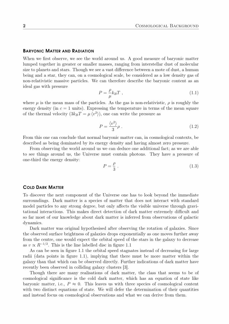
Dark matter was original hypothesised after observing the rotation of galaxies. Sincethe observed surface brightness of galaxies drops exponentially as one moves further awayfrom the centre, one would expect the orbital speed of the stars in the galaxy to decreaseas v ∝ R−1/2. This is the line labelled disc in figure 1.1
As can be seen in figure 1.1 the orbital speed stagnates instead of decreasing for largeradii (data points in figure 1.1), implying that there must be more matter within thegalaxy than that which can be observed directly. Further indications of dark matter haverecently been observed in colliding galaxy clusters [3].
Though there are many realisations of dark matter, the class that seems to be ofcosmological significance is the cold dark matter, which has an equation of state likebaryonic matter, i.e., P ≈ 0. This leaves us with three species of cosmological contentwith two distinct equations of state. We will defer the determination of their quantitiesand instead focus on cosmological observations and what we can derive from them.
Cosmological Principle and the FRW Metric 3
Figure 1.1: Rotation curve data from NGC3198 along with fits for dark matter profile.Taken from [4]
Part of the dark matter comes from neutrinos, which are, in the ΛCDM model, treatedas ultra-relativistic particles. They will therefore contribute to the radiation term.
1.2 COSMOLOGICAL PRINCIPLE AND THE FRW METRIC
Having observed the matter and radiation of the Universe, we can apply these initialobservations to paint the characteristics of the Universe with a broad brush. Doing a fullsky survey of the radiation, one finds first of all that there is a microwave background,which exhibits a remarkably perfect black body spectrum with a peak at a temperatureof about 2.73K (see figure 1.2 on the following page).

4 Cosmological Background
Figure 1.2: Black body spectrum of the CMB by the COBE satellite. From [5]
Comparing this result with a map of how the temperature varies over the sky (seefigure 1.3. Note that the variations are of the order of 0.1 mK), one notices that theobserved radiation is astoundingly isotropic.
Figure 1.3: Full sky map by the WMAP satellite after subtraction of galactic foreground,mean temperature and dipole contribution. From [6]

Cosmological Principle and the FRW Metric 5
If one furthermore maps out the matter distribution on large scales, it emerges that onlarge scales the distribution of galaxies can be seen to be both isotropic like the CosmicMicrowave Background (CMB), as well as homogeneous. These observations support whatis known as the cosmological principle; that the Universe can, on scales larger than roughly100 Mpc, be regarded as homogeneous and isotropic.
COSMOLOGICAL DYNAMICS
At these length scales gravitation dominates the other fundamental forces, making it pos-sible to describe the dynamics of the Universe on cosmological scales by the general theoryof relativity. Invoking general relativity one can write down the Friedmann-Robertson-Walker (FRW) metric as the most general metric, which obeys the cosmological principle:
ds2 = −dt2 + a(t)2[dr2 + Sκ(r)
2(dθ2 + sin2(θ)dφ2
)](1.4)
with
Sκ(r) =
R0 sin(r/R0) κ = 1 (Closed universe/positive curvature)r κ = 0 (Flat universe)R0 sinh(r/R0) κ = −1 (Open universe/negative curvature)
. (1.5)
Here R0 is the curvature radius of the Universe. Inserting the FRWmetric into the Einsteinequation one finds the Friedmann equation from the 00-component, which connects theevolution of the scale factor a(t) to the content of the Universe and its curvature:
H2 ≡(a
a
)2
=ρ
3− κ
R20a(t)2
. (1.6)
This serves as a definition of the Hubble parameter, H, which quantifies the relativeexpansion rate of the Universe, while ρ denotes the total energy density of the Universe.Solving the Friedmann equation in conjunction with the continuity equation
ρ+ 3H(ρ+ P ) = 0 , (1.7)
one can find the evolution of the scale factor as a function of the physical time. For thetwo components (we will from now on regard baryonic matter and cold dark matter asparts of the same component, i.e., cold matter which exerts negligible pressure) introducedearlier, one can solve eq. 1.7 to find
ρ(a) = ρ(a0)
(a0
a
)3 cold matter(a0
a
)4 radiation. (1.8)
One could easily have argued that the energy densities should depend on the scale factorin this fashion. Both components are diluted as the Universe expands giving an a−3
dependence. The extra factor a−1 for the radiation comes from the red shifting of thephotons as they travel through an expanding space.
In addition to the two components already introduced there is a third component,which will play a key role throughout this work. That is a component with a constantenergy density. Assuming this, one finds from eq. 1.7 that such a component exerts

6 Cosmological Background
negative pressure: P = −ρ. Sometimes named a cosmological constant or dark energy, aflat universe dominated by this will have a constant Hubble parameter and will thereforeexpand exponentially. Such a universe, called a de Sitter space, will play an integral rolein the following chapters.
Defining the critical density of the Universe (ρc,0) as the one needed for making a flatuniverse (κ = 0), one can express the present day value as
ρc,0 = 3H20 , (1.9)
where H0 is the present value of the Hubble parameter. Collecting the results derived thusfar, one can write the Hubble parameter as
H2 = H20
[Ωr,0
a4+
Ωm,0
a3+ ΩΛ,0 +
1− Ω0
a2
]. (1.10)
In the above and for the rest we have set a0 = 1 as the present day value of the scale factorand written the energy densities as fractions of the critical energy density today:
Ωi,0 ≡ρi,0ρc,0
, Ω0 ≡∑i
Ωi,0 . (1.11)
The four terms in eq. 1.10 are radiation, cold matter, cosmological constant and curvature,respectively. We have anticipated events slightly by adding the cosmological constant term,even though it has not, at this point, been argued to be part of our universe. One shouldbear in mind that there is so far no physical explanation for this term, and it acts merely asa placeholder needed to describe the observations. One can find many possible realisationsthat fulfil the observed properties (see [7] and references within).
To determine the evolution of the Universe, one now needs to fix the parameters byobservation.
1.3 BASICS OF MEASUREMENTS
Starting from the little we know at present, we utilise the fact that most of the photonsin the Universe are part of the CMB, which has a black body spectrum (see figure 1.2on page 4). One can therefore estimate the energy density of radiation from Stefan-Boltzmann’s law and find
Ωγ,0 = 2.469× 10⁻⁵h−2 , h ≡ H0
100km/s/Mpc. (1.12)
The notation Ωγ,0 denotes purely the photon contribution. The total contribution to theradiation energy density also includes neutrinos, which will not be discussed in detail inthis work.
This result is fairly independent of the model assumptions as opposed to the other cos-mological parameters. One should therefore start with reviewing the methods of observa-tion and the notion of scales that is employed, when one fixes the cosmological parameters.
As observers of the Universe we are limited by the fact, that we can only observelight and particles that come to us. This results in a set of data that not only has theimprint of the original source, but also holds information about anything that is passed

Measuring the Geometry of the Universe 7
on the way from the source to the observer. To complicate matters further, one cannotrely on the measurement of a well-defined physical distance (the coordinate distance ofthe FRW-metric), as this is prohibited by causality in an expanding universe.
To establish a distance measure one defines the luminosity distance in terms of themeasured flux, f , and luminosity of a source, L, which can usually be inferred by someother methods:
dL ≡(
L
4πf
)1/2
. (1.13)
One should note that this quantity only corresponds to the physical distance in a static,Euclidian, three dimensional space.
In a universe with a FRW metric of general curvature the geometry and expansionmanipulates the perceived flux from a source. This is caused by three different effects onthe photons emitted from the source. Firstly the area over which the photons are spread,given by
Aκ(r) = 4πSκ(r)2 (1.14)
changes with the curvature of the Universe. Secondly the photons are redshifted, dimin-ishing the energy of the photon by a factor of of (1 + z)−1, where z is the redshift ofthe source. Lastly, two photons emitted a time ∆t apart will arrive with an interval of∆t(1 + z) due to the expansion, contributing another factor of (1 + z)−1 to the flux:
f =L
4πSκ(r)2(1 + z)2. (1.15)
This leads to a luminosity distance of
dL = (1 + z)Sκ(r) . (1.16)
1.4 MEASURING THE GEOMETRY OF THE UNIVERSE
As the curvature of the Universe plays such an immense role in our perception of distance,it should be one of the first parameters we attempt to determine. Though it cannot bedone in a completely model independent way, it can be found almost independent of theother cosmological parameters.
Measuring the anisotropies of the CMB and fitting the measured power spectrum1 toa theoretical one, will not only allow us to infer Ω0, but also give us an estimation ofthe other cosmological parameters. There are, however, still a fairly large solution spaceallowed from the CMB data alone. One therefore needs further data to pin down thecorrect values of the cosmological parameters. This will be illuminated in the followingsection.
Exploiting the information in the CMB anisotropies requires a little knowledge of thehistory of the Universe. Based on repeated observations of objects on the cosmologicalscales it is concluded that the Universe is expanding. This implies that the Universemust at some point have started from a hot, dense state. As the Universe expanded, theequilibrium between baryons, leptons and photons shifted until atoms started forming inthe recombination epoch, making the Universe electrically neutral. This was followed by
1A more thorough definition of the power spectrum will be presented in chapter 3 on page 21
8 Cosmological Background
the photon decoupling epoch, which occurred when the expansion of the Universe came todominate the photon-electron scattering rate. Shortly after this the mean free path of thephotons grew to make them free stream, marking the last scattering surface which we nowobserve as the CMB. One of the more notable things about the last scattering surface,is that the redshift at which it takes place, 1 + zls ≈ 1100, is nearly independent of thecosmological parameters. This makes it ideal for observing the curvature of Universe.
If one observes two fluctuations in the CMB that were a physical distance l apart onthe last scattering surface, one would observe them to have an angular distance of
∆φ =l
a(tls)Sκ(r)=l(1 + zls)
2
dL. (1.17)
Whereas the numerator is largely independent of the chosen cosmology, the denominatordepends on the geometry of the Universe as dL becomes smaller in a closed universe andlarger in an open. Thus
∆φopen < ∆φflat < ∆φclosed . (1.18)
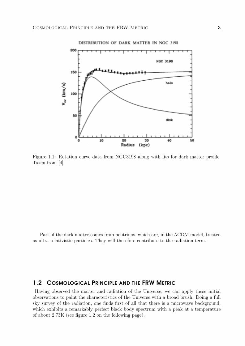
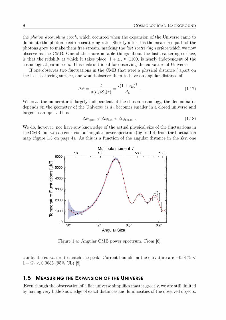
We do, however, not have any knowledge of the actual physical size of the fluctuations inthe CMB, but we can construct an angular power spectrum (figure 1.4) from the fluctuationmap (figure 1.3 on page 4). As this is a function of the angular distance in the sky, one
Figure 1.4: Angular CMB power spectrum. From [6]
can fit the curvature to match the peak. Current bounds on the curvature are −0.0175 <1− Ω0 < 0.0085 (95% CL) [8].
1.5 MEASURING THE EXPANSION OF THE UNIVERSE
Even though the observation of a flat universe simplifies matter greatly, we are still limitedby having very little knowledge of exact distances and luminosities of the observed objects.

Measuring the Expansion of the Universe 9
One way to resolve this problem is to look for standard candles. These are objects thatall have the same luminosity independent of the redshift at which they are observed.
The preferred standard candle of cosmology is the type Ia supernova, which is extremelyluminous and have adequately known properties. Originating from a binary system wherea white dwarf accretes matter from a companion star, the white dwarf will collapse whenits mass exceeds the Chandrasekhar limit of 1.4 M. Though the luminosities of thesesupernovae vary slightly (around (3− 5)× 109L), they have been found to obey redder-dimmer and wider-brighter relations, which makes it possible to find the luminosity of thesupernova. See figure 1.5 from [9] and further references therein for details. To relate the
Figure 1.5: Observed magnitudes and model for eight supernovae [9]
luminosities and the measured redshift to the expansion of the Universe, one comparesobservations to a model universe and perform a complete statistical analysis. We willdemonstrate the principles here by limiting the analysis to observations of the recent past,i.e., very low redshifts.
Expanding the scale factor to the second order around present day (t0), one finds
a(t)
a(t0)≈ 1 +H0(t− t0)− q0
2H2
0 (t− t0)2 (1.19)
where we have defined the deceleration parameter
q0 = −1−
(H
H2
)t=t0
= Ωr,0 +Ωm,0
2− ΩΛ,0 . (1.20)

10 Cosmological Background
Measuring this parameter gives us the means to determine Ωm,0 and ΩΛ,0 in combinationwith the CMB anisotropy data. In order to couple redshift and luminosity distance, weuse the fact that the Universe is approximately flat at the distances we consider, making
dL(t0) = (1 + z)dp(t0) = (1 + z)
∫ t0
te
dt
a(t)≈ (1 + z)
[(t0 − te) +
H0
2(t0 − te)2
](1.21)
to the second order in t0− te. Here dp(t0) is the physical distance a photon, emitted at te,has travelled at the time t0. Inverting 1
a(t)= 1 + z one finds
dL(z) ≈ z
H0
(1 +
1− q0
2z
)(1.22)
to the second order in z. Expressing the observations in distance modulus
m−M = 5 log10
(dL
1Mpc
)+ 25 , (1.23)
one finds a simple relation between the distance modulus and the redshift:
m−M ≈ 45.33− 5 log10
(H0
70km/s/Mpc
)+ 5 log10(z) + 1.086(1− q0)z , (1.24)
under the assumption that 1−q02z 1. Using this relation in conjunction with the CMB
data, one can fit the cosmological parameters. Figure 1.6 on the next page shows the resultfrom a full analysis. The difference in the theoretical curve in the figure and the relationfor low redshifts comes from plotting a corrected version of the distance modulus, whichtakes systematic errors and light absorption from dust between source and observer, andother effects as well into account(see [9] for details).
1.6 RECAPPING THE UNIVERSE
Combining the discussed observations with observation of Baryon Acoustic Oscillations(BAO), one can tightly constrain the cosmological parameters and give a reasonable de-scription of the history of the Universe. The BAO are the result of temperature fluctua-tions in the primordial plasma, making the photon-baryon gas expand and thus sendingan acoustic wave through the plasma. This creates a spherical sound wave through thebaryons and photons, leaving the dark matter untouched. This happens at every overden-sity resulting in a wave pattern, which can be observed in the distribution of galaxies. Thegrowth of these sound horizons stops at the time of photon decoupling as the interactionsbetween photons and baryons stops, relieving the pressure of the system. As the soundwaves imprints themselves on the structure formation, this makes for a standard ruler thatis approximately 150 Mpc today [10].
From the three measurements (drawn in figure 1.7 on page 12) one can compile a bestfit to the cosmological model of eq. 1.10 on page 6 with [8]:
Ωr,0 = Ωγ(1 + 0.2271Neff) = 8.49× 10⁻⁵
Ωm,0 = Ωb,0 + Ωc,0 , Ωb,0 = 0.0462± 0.0015 , Ωc,0 = 0.233± 0.013
ΩΛ,0 = 0.721± 0.015
H0 = 70.1± 1.3km/s/Mpc
(1.25)

Recapping the Universe 11
Figure 1.6: Binned Hubble diagram from [9]. Bottom shows residuals from best fit
One should note that the effects of neutrinos are taken into account in the radiation termwith Neff = 3.04 as the standard value.
One can thus summarise the history of the Universe: Starting from a hot dense state,the Universe expanded and cooled. After a time the plasma had cooled enough for atomsto form. This recombination epoch was followed by the photon decoupling epoch whenscattering rate for photon-electron scattering becomes lower than the Hubble parameter.

12 Cosmological Background
Figure 1.7: Plot of Ωm,0 vs. ΩΛ,0 with 1σ, 2σ and 3σ confidence intervals. From [9]
Shortly after this decoupling the mean free path of the photons became so large, that thephotons could free stream from the time of the last scattering surface. As the expansioncontinued matter began to cluster and form the structures we observe today in our flat,homogeneous and isotropic Universe.
Though this is a nice scenario, there are still some issues in the hot Big Bang scenario,that needs to be addressed. This will be done in the following chapter.

2 ISSUES WITH THE BIG BANG SCENARIO
Though the ΛCDM-model provides a good explanation of the data (see figures 1.4and 1.7), certain aspects of it may be slightly disturbing. These will need to be addressed,if one is to accept the ΛCDM-model. The following paragraphs are based on [1, 2, 11, 12].
2.1 THE FLATNESS PROBLEM
Fits to data show that the Universe is flat (Ω0 = 1) to within a few per cent. One wouldnot usually take a fine tuning to within a few per cent to be a major concern, but oneshould bear in mind that the deviation from a flat universe should be extremely small atthe time of Big Bang Nucleosynthesis (BBN) in order to give an Ω0 so close to 1 today.
If one regards the total relative energy density (Ω0) as a function of the scale factor
Ω0(a) =ρ
3H2= 1 +
κ
(aH)2R20
, (2.1)
one sees that |Ω(a)− 1| grows through matter (w = 0) and radiation (w = 13) dominated
epochs as (aH)2 ∝ a−1 and (aH)2 ∝ a−2, respectively. Taking matter-radiation equality tobe around redshift of 1 + zeq ∼ 3600 and BBN around redshift 1 + zBBN ∼ 1010, one findsΩ(aBBN)− 1 ∼ 10−18 at the time of BBN in order to meet the observational constraints.
This seems highly unlikely and requires a great deal of fine-tuning of the initial param-eters. Hence he Flatness Problem arises as a fine-tuning problem. An illustration of thecurvature is provided in figure 2.1 on the following page.
2.2 THE HORIZON PROBLEM
If one further regards the fundamental assumption for the FRW universe, one encountersa second problem with the hot Big Bang model described previously. This fundamen-tal assumption, the cosmological principle, states that the Universe is, on large scales,homogenous and isotropic, which does indeed seem to be in agreement with the measure-ments. The observations of the CMB have, in fact, limited the relative variations in theCMB temperature to be of the order 10−5. This is particularly remarkable when one com-pares the distance a light signal could travel before decoupling to the size of the horizon.Assuming, for the sake of simplicity that recombination and the generation of the lastscattering surface coincides, one can find the travelled distance to be
L = arec
∫ trec
0
dt
a(t)= 2trec = H−1
rec = H−10 (1 + zrec)
−3/2, (2.2)

14 Issues with the Big Bang Scenario
Figure 2.1: Sketch of the evolution of the curvature term through a radiation and a matterdominated period
where the last equality assumes a matter dominated universe from recombination untilpresent day.
This should be compared to the size of the last scattering surface at the time of recom-bination (assuming a flat geometry):
D =areca0
a0
∫ t0
trec
dt
a(t)= (1 + zrec)
−1 2
H0
[1− (1 + zrec)
−1/2]. (2.3)
Comparing the two results, one finds that the maximum angular distance between twocorrelated points in the sky to be
θ =L
D' 1
2(1 + zrec)
−1/2 ≈ 1 . (2.4)
That is to say, any two photons coming from more than 1 apart have never been causallyconnected, making it quite remarkable that the CMB is so homogeneous. The HorizonProblem is illustrated in figure 2.2 on the next page. The diagram shows clearly thattwo points on the last scattering surface have past light cones that never overlap. Theycan therefore not have been in casual connection with one another prior to the photondecoupling epoch.
2.3 A POSSIBLE SOLUTION TO BOTH PROBLEMS
Alan H. Guth pointed out in 1981 [14] that one could solve both problems by introducingan epoch of accelerated, or inflationary, expansion in the early universe. Though this ideais remarkably simple from a conceptual point of view, it solves the Flatness Problem andthe Horizon Problem quite effectively, provided that it goes on for a long enough time.

A Possible Solution to Both Problems 15
Figure 2.2: Spacetime diagram of the evolution of the Universe with past light cones oftwo points marked in yellow. Last scattering surface is marked with a blue line. Takenfrom [13]
In the case of the Flatness Problem the inflationary expansion needs to provide Ω(aBBN)−1 ∼ 10−18 at the time of BBN. Since nuclei start to form at around a temperature ofTBBN ∼ 1 MeV, one can estimate the required time for solving the Flatness Problem byestimating the energy scale of the end of inflation to be around TI ∼ 1015 GeV and as-suming a radiation dominated universe from the end of inflation to the time of BBN, onegets
Ω0(aI)− 1 ∼ (Ω0(aBBN)− 1)
[aI
aBBN
]2
(2.5)
from eq. 2.1 on page 13. As T ∝ a−1 one can rewrite this to
Ω0(aI)− 1 ∼ 10−54
[1015 GeV
TI
]2
. (2.6)
Though an initial condition of 10−54 may seem impossibly small, this is easily manageableby assuming a nearly exponential growth factor, i.e., an approximate de Sitter solution.In this case the Hubble parameter is nearly constant and one can write
(aH)f(aH)i
' afai
= e∆N , (2.7)
where the number of e-folds ∆N has been introduced. In this case one only needs
∆N =1
2ln(1054) ' 62 (2.8)
to provide a sufficiently flat initial condition to meet the current observational bounds (cf.eq. 2.1 on page 13).
For the Horizon Problem the issue was that any two points more than a degree apartin the sky could not be causally connected. Recasting this problem to one of length scalesit means that the physical length L = a(t)l has been larger than the Hubble length H−1
previous to recombination. For the largest scales we can observe today (l ∼ (aH)−10 ), this

16 Issues with the Big Bang Scenario
means that the ratio between the physical length scale and the Hubble length at the timeof BBN was
LBBN
H−1BBN
= l(aH)BBN =(aH)BBN(aH)eq
(aH)eq(aH)0
. (2.9)
Again assuming a universe dominated by radiation from the time of BBN to the the timeof matter-radiation-equality and matter dominated from then till present day, one gets
LBBN
H−1BBN
∼ 108 . (2.10)
As aH grows during the inflationary epoch, a sufficient period of inflation will ensurethat all observable length scales have at one point been smaller than the Hubble length.Requiring that the largest length scales today have at one point been the size of the Hubblelength (a∗l = H−1
∗ ), one finds
1 =(aH)0
(aH)∗=
(aH)end(aH)∗
(aH)eq(aH)end
(aH)0
(aH)eq(2.11)
with the assumption of an instant transition from the end of inflation to BBN. Here thesubscript end marks the end of inflation. If the matter-radiation-equality occurs at atemperature of Teq ∼ 3 eV, one can estimate
(aH)eq(aH)end
=aendaeq
=TeqTI
= 3× 10⁻²⁴ 1015 GeV
TI. (2.12)
Making the same assumption of a nearly exponential growth during inflation, one can findthe required number of e-folds, such that the largest observable length scales must havebeen equal to the Hubble length to be
∆N ∼ 58 + ln
(TI
1015 GeV
). (2.13)
Sketching the curvature term as in figure 2.3 on the facing page one can see, how infla-tion solves the Flatness Problem and the Horizon Problem. By extending the inflationaryepoch, one can achieve the initial curvature needed to match the present observationalbounds.
2.4 INFLATION AT A GLANCE
To achieve and sustain inflation long enough to solve the Flatness Problem and theHorizon Problem, one needs to set up a scenario in which the Universe accelerates andcontinues to do so for the required number of e-folds. One can parameterize this accelera-tion and its stability through the slow-roll parameters, which can be defined by regardingthe acceleration requirement
0 <a
a= H +H2 ⇔ ε ≡ − H
H2< 1 , (2.14)
i.e., one has an accelerated expansion as long as the first slow-roll parameter ε is sufficientlysmall. In order to sustain inflation ε should remain small, i.e., the relative change in ε

Inflation at a Glance 17
Figure 2.3: Sketch of the evolution of the curvature term through a radiation and a matterdominated period, preceded by a period of inflation
should mostly be small compared to the expansion rate, which yields the definition of thesecond slow-roll parameter:
η ≡ ε
Hε 1 . (2.15)
One can estimate an upper bound on the slow-roll parameters, which should be obeyed toachieve the desired number of e-folds:
ε = − H
H2= −HN
H, (2.16)
where the index N denotes a derivative with respect to the number of e-folds. One canapproximate this as HN ∼ ∆H
∆N, where the change of the Hubble parameter −∆H < H.
This gives
ε < ∆N−1 ∼ 1
60. (2.17)
The same argument can be applied to η to find the same bound on the second slow-rollparameter.
Achieving the low values of the slow-roll parameters in the first place is no simple feat,and is highly dependent on the chosen model. In many toy models this reintroduces a levelof fine-tuning, and even in more elaborate high energy theories, e.g. string theory, it is notgeneric that the slow-roll parameters are small. This is sometimes known as the η-problemin string theory, in which suppressed corrections to the model lead to contributions to ηof order 1, thus hindering sustained inflation.
The numerical calculations in this work will always assume that both slow-roll param-eters are initially small.

18 Issues with the Big Bang Scenario
Expressing the slow roll condition in terms of the fields involved, it means that thefields driving the cosmological expansion should have a negligible kinetic energy, i.e., theirpotential should be nearly flat.
At some point inflation ends by breaking slow-roll, i.e. the fields reaches a segmentwhere the kinetic energy of the inflaton becomes comparable to its potential energy.Shortly after that, the inflaton field begins to oscillate around a minimum in the po-tential. At this point the energy density should be transferred from the inflaton to thematter fields we observe today, a scheme generally referred to as reheating.
This can be achieved in many ways, but is in general described as a two stage process,where the first step (called pre-heating) is an explosive depletion of the energy density ofthe inflaton to produce an intermediary field χ, followed by a decay of the χ particles tostandard model particles and a subsequent or simultaneous thermalisation of the particleproducts. The original example [15], which will be shortly reviewed here assumes that theinflaton, φ, couples to a bosonic field χ and a fermionic field ψ through
Lint = −1
2g2φ2χ2 − hψψφ , (2.18)
where h, g 1. The further details of pre-heating depend on the potential for the inflaton,but in general it is the oscillations of the inflaton fields around the minimum, that excitesthe bosonic field. In the case of a decay purely to fermionic particles, reheating completeswhen the decay rate is comparable to the Hubble parameter.
As reheating ends and the radiation dominated period initiates, the last effect of in-flation kicks in. The fluctuations of the inflaton field have embedded themselves in thespacetime and afterwards been carried outside the Hubble horizon, due to the expansionof the Universe. As the acceleration stops the horizon starts to expand faster than theUniverse, making the fluctuation reappear inside the horizon. These fluctuations acts asperturbation seeds in the self-gravitating fluid, which exists in the Universe.
Expressing the density contrast δρMρM
in terms of its Fourier transform
δρMρM
=
∫d3kδk(t)e−ik·x , (2.19)
one can write down the evolution of the density contrasts by a Newtonian equation:
δk + 2Hδk +
(∂p
∂ρM
)2k2
a2δk = 4πGρMδk . (2.20)
Solving this for the radiation and matter dominated epochs, one finds δk ∝ ln(a) andδk ∝ a, respectively. Thus one will only see a real growth in overdensities during thematter dominated epoch.

Inflation at a Glance 19
Figure 2.4: Observations of the galactic distribution from 2dFGRS [16] and the SDSS [17],compared to N -body simulation. Figure from [18]
Once the overdensities becomes of order unity, they decouple from the expansion,becoming their own self-gravitating system and begin the process of virial relaxation.These will eventually make up the structure, that we see in our Universe today (see figure2.4 for a comparison between observation and simulation of large scale structure). This,however, leaves the question of the origin and properties of the initial fluctuations; thescope of this thesis.

20 Issues with the Big Bang Scenario

3 STATISTICS AND PERTURBATION THEORY
To drive the Universe through an inflationary stage, one usually needs to invoke a highenergy quantum field theory or a theory of quantum gravity. As such quantum fluctuationsarise as a natural part of inflation.
One therefore needs a framework to understand the effects of these fluctuations on theunderlying metric, as well as a definition of the suitable statistics needed to describe theperturbations of the metric and how these statistics are linked to the chosen theory ofinflation.
This chapter is dedicated to a review of the necessary statistics and first order per-turbation theory. Higher order perturbation theory is deferred to chapter 8. Most of thederivations are inspired by [11].
3.1 METRIC PERTURBATIONS
Though it might not be evident from the beginning that the quantum fluctuations inthe fields driving inflation are tightly linked to the perturbations of the metric, one canconstruct a simple argument to illustrate this connection qualitatively.
A fluctuating set of fields will, through their contributions to the energy-momentumtensor, introduce a perturbation of the same tensor δTµν . This couples to the metric tensorthrough the Einstein equation:
δTµν = δ
(Rµν −
1
2gµνR + Λgµν
)∝ δgµν . (3.1)
The reverse effect can also be seen as the metric tensor enters in the equation of motiongoverning the fields of the theory, e.g., the Dirac or Klein-Gordon equation. Thus aperturbation of the metric tensor will invariably translate into a fluctuation of the fields.
Writing the metric as sum of an unperturbed background and a general perturbation
gµν = g(0)µν + δgµν , (3.2)
one usually chooses the background to be the FRW metric (c.f. 1.4 on page 5). Theperturbation can be broken down to a combination of scalar modes, vector (or vorticity)modes and tensor (or gravitational wave) modes. The latter occur as a physical degreeof freedom in the sense that they can exist independently of the content of the Universe,and even exist in vacuum. The scalar and vector modes will only arise in conjunction withfluctuations of the fields in the Universe.

22 Statistics and Perturbation Theory
It can be instructive to commence the discussion about metric perturbation by in-ventorying the degrees of freedom (DOF) available within each type of mode in a n + 1dimensional metric. As the metric must be symmetric, one is left with 1
2(n + 2)(n + 1)
DOF in δgµν (n+1 from the diagonal and 12n(n+1) from the off diagonal triangle, picture
(a) in figure 3.1). One can now eliminate n + 1 of these by coordinate transformationsand write the remaining as a scalar, a n dimensional vector and a n× n symmetric tensor(picture (b) in figure 3.1).
Figure 3.1: Graphical representation of decomposing the metric perturbations
By Helmholtz’s theorem one can decompose the vector into a scalar and a divergencefree vector (ui = ∂iv + vi), leaving n− 1 vector degrees of freedom due to the divergencecondition.
Regarding the tensor modes, one can repeat the above argument to find that the sym-metry requirement constrains the DOF to 1
2n(n+ 1). Imposing the additional constraints
of the tensor modes being traceless and transverse (∇iδgij = 0) removes n + 1 DOF; onefrom being traceless and n from requiring it to be transverse. This leaves 1
2(n− 2)(n+ 1)
tensor DOF.From this it is now possible to find the total number of scalar DOF to be
1
2(n+ 2)(n+ 1)︸ ︷︷ ︸
Total DOF
− (n+ 1)︸ ︷︷ ︸Coordinate transformations
− (n− 1)︸ ︷︷ ︸Vector DOF
− 1
2(n− 2)(n+ 1)︸ ︷︷ ︸
Tensor DOF
= 2 . (3.3)
The next section will be dedicated to writing down the specific perturbations for the FRWmetric.
3.2 PERTURBING THE FRW METRIC
Considering the 3 + 1 dimensional flat Friedmann-Robertson-Walker metric
ds2 = −dt2 + a(t)2ηijdxidxj , (3.4)
it is possible to introduce perturbations, by following the classic paper [19]. We limitourselves to a flat space with only scalar perturbations in the following. The most general

Perturbations in Single Field Inflation 23
first order scalar perturbation of eq. 3.4 one can write down is
ds2 = −(1 + 2A)dt2 + 2∂iBdtdxi + a(t)2((1 + 2ψ)ηij +DijE)dxidxj (3.5)
withDij = ∂i∂j −
1
3ηij∂
2 . (3.6)
These perturbations cannot, however, be independent as it was shown above that thetotal number of scalar degrees of freedom in the system is 2. The two physically relevantperturbations are known as Bardeen’s potentials (introduced in [20, 21]). To derive theseone can perform a gauge transformation (again regarding solely the scalar contribution)
t→ t+ ξ , xi → xi + ∂iβ , (3.7)
and require that the line element, truncated to the first order in this case, is invariant undercoordinate transformation. Denoting the perturbation parameters after the coordinatetransformation with a tilde, one get
ds2 →− (1 + 2(A+ ξ))dt2 + 2∂i(B − ξ + a2β)dtdxi
+ a(t)2
[(1 + 2(ψ +Hξ +
1
3∂2β))ηij +Dij(E + 2β)
]dxidxj .
(3.8)
From this one can deduce from eq. 3.5 that
A =A− ξ (3.9)
B =B + ξ − a2β (3.10)
ψ =ψ −Hξ − 1
3∂2β (3.11)
E =E − 2β . (3.12)
From these transformations one can now construct the two Bardeen’s potentials (Φ andΨ):
Φ =A+d
dt
(B − Ea2
2
)(3.13)
Ψ =ψ +∂2E
6+H
(B − Ea2
2
)(3.14)
The exact expressions for these gauge invariant perturbations are highly dependent onthe choice of time coordinate, as different choices correspond to different hypersurfaces ofconstant time (time slices).
3.3 PERTURBATIONS IN SINGLE FIELD INFLATION
Limiting the discussion for a moment to model with a single scalar field, we introducethree standard gauge choices: The isocurvature gauge, the comoving curvature gauge andthe uniform curvature gauge. Each hold its own virtues and will be briefly reviewed.

24 Statistics and Perturbation Theory
The discussion requires a knowledge of transformation laws for perturbed scalar quan-tities. We follow the pedagogical derivation from [11]:
Transforming the coordinate system from xµ → xµ = xµ + δxµ, one transforms theperturbation of a scalar quantity f as δf(xµ)→ δf(xµ). As
δf(xµ) = f(xµ)− f0(xµ) , (3.15)
where f0 is the background quantity, we can rewrite this as
δf(xµ) = f(xµ)− f0(xµ) , (3.16)
since f(xµ) is a physical scalar, i.e. it is independent of the choice of coordinate system.Expanding f(xµ) around xµ yields
δf(xµ) = f(xµ)− f0(xµ)− ∂f
∂xµδxµ = δf(xµ)− ∂f
∂xµ xµ=xµδxµ . (3.17)
The curvature referred to in the names of the perturbation choices is the perturbationparameter ψ. This is simply due to, that the intrinsic curvature scalar for the spatial partof the metric is given by
R3 = − 4
a2∇2ψ (3.18)
ISOCURVATURE GAUGE
The isocurvature perturbation distinguishes itself from the other two by having the pertur-bations solely in the field fluctuations, providing a scheme with nice features for performingslow roll computations, i.e., computations when ε, η 1.
Requiring the spatial perturbations to vanish, we perform a time translation as wasdone in eq. 3.7 on the preceding page:
ψ = ψ −Hξ = 0⇒ ξ =ψ
H. (3.19)
Performing the same time translation on the field fluctuation, gives rise to the Mukhanov-Sasaki variable
Q = δφ− φ
Hψ , (3.20)
which is gauge invariant and identical to δφ, when the spatial perturbations go to zero.
COMOVING CURVATURE GAUGE
Observers in the comoving picture will see themselves as free falling, making the expansionseem isotropic, meaning that they do not measure any energy flux (Ti0 = 0). For thecanonical single field case, one gets
Ti0 ∝ φ∇iδφ , (3.21)
meaning that the time translation should take δφ→ 0. That is
δφ→ δφ− φξ = 0 (3.22)

Statistics in Expanding Spacetime 25
for the time translation t→ t+ ξ, meaning that ξ = δφ
φ. This transformation gives
ψ → R ≡ ψ −Hδφ
φ, (3.23)
which is gauge invariant. This quantity R is the comoving curvature perturbation, whichis equal to the gravitational potential, when one transform to hypersurfaces where δφ = 0.
UNIFORM DENSITY GAUGE
In single field inflation the choice of δφ = 0 implies both comoving curvature perturbationsand uniform density perturbations, the definition of the two are however different. For theuniform density perturbations one does a time translation t → t + ξ, such that δρ → 0,i.e.,
δρ→ δρ− ρξ = 0 . (3.24)
This transformation brings ψ to
ψuni = ψ −Hξ = ψ −Hδρ
ρ≡ ζ . (3.25)
As we are dealing with a single field, one can write
δρ = φ ˙δφ+ V ′(φ)δφ . (3.26)
For the general single field slow roll scenario, one can, on superhorizon scales (k H),reduce the equation of motion to
3Hφ+ V ′ ' 0 , (3.27)
giving the first order expression
˙δφ ∝ (slow roll parameters)Hδφ , (3.28)
which reduces δρ toδρ ' V ′δφ . (3.29)
One can now use the fluid equation (eq. 1.7 on page 5) to rewrite
ρ = −3H(ρ+ p) = −3Hφ2 ' V ′φ . (3.30)
This totals toζ ' ψ −Hδφ
φ= R . (3.31)
One sees that on superhorizon scales the comoving curvature perturbations and the uniformdensity perturbations reduce to the same quantity.
3.4 STATISTICS IN EXPANDING SPACETIME
As one does not observe the perturbations directly, but more the statistical properties of

26 Statistics and Perturbation Theory
the perturbations, one should define the general statistical tools needed to describe theperturbations.
The pivotal ingredient for discussing the properties of a perturbation is the n-pointcorrelation function, written as 〈Ξn〉 for a stochastic variable Ξ, where the brackets denotethe vacuum expectation value. This n-point correlation function can in some cases bewritten in a simple way. In inflation, however, one keeps things simple by distinguishingbetween such a simple case (Gaussian) and a deviation from this case (non-Gaussian). Forthe Gaussian case one can write
〈Ξn〉 =
n!
2n/2(n2 )!〈Ξ2〉n/2 for n even
0 for n odd. (3.32)
That there is a one-to-one correspondence between following a Gaussian distribution andobeying eq. 3.32 come from the fact that any distribution is uniquely determined by itsmoments, i.e., its n-point correlation functions.
One can thus determine if an operator is non-Gaussian by measuring a deviation fromeq. 3.32. In the coming we will concern ourselves mainly with the three-point function andthe four-point function.
In calculating the n-point function in an expanding spacetime, one is faced with certaindifficulties as the vacuum state is not well defined. To work around this issue one formulatesthe problem in the Heisenberg picture and evolves the vacuum state from a known initialcondition. Thus:
〈Ξn〉 =⟨
Ω eR
d4x′HI(x′)ΞnI e−
Rd4x′HI(x′) Ω
⟩' 〈Ω Ξn
I Ω〉
− i∫
d4x′ 〈Ω [ΞnI ,HI(x
′)] Ω〉 .
(3.33)
Thus one has a direct influence of the model, through the interaction Hamiltonian, onthe n-point correlation function. This makes it possible to compare the observed spectraand theoretical calculations via the relevant correlation functions.
Most of the time, however, one expresses the calculated correlation functions in termsof spectra. First introduced in the field of signal processing, the concept applies nicely tothe perturbations that occurs during inflation.
SPECTRA
Starting from the two-point function one defines the power spectrum as the autocorrela-tion function of the stochastic operator (operators are denoted with capitals, while modefunctions are denoted with small case):⟨
Ξ2⟩
=
∫d3kd3k′ 〈Ξ(k)Ξ(k′)〉 e−i(k+k′)·x
= (2π)3
∫d3k|ξk|2
= 4π(2π)3
∫dkk2|ξk|2
≡ (2π)6
∫dk
kPΞ(k) .
(3.34)

Statistics in Expanding Spacetime 27
Here we have used the decomposition of the operator into raising and lowering operators
Ξ(k) = ξkak + ξ−ka†−k (3.35)
with the normalisation
[ak, ak′ ] = [a†k, a†k′ ] = 0 , [ak, a
†k′ ] = (2π)3δ(3)(k − k′) , (3.36)
This gives an equivalent, and for the purposes in this work, more useful definition:
PΞ(k) =k3
2π2|ξk|2 . (3.37)
As will be shown in eq. 4.22 on page 33, the power spectrum of single field inflation isnearly scale invariant, i.e. independent of k.
0 2 4 6 8 10 12 14
0.4
0.5
0.6
0.7
0.8
0.9
1.0
|x-y|
Correlation
Figure 3.2: Cartoon of correlation function with the ”data set” (the arrows) displayedbelow
From figure 3.2 one can get an impression of the information stored in a two-pointcorrelation function, and through that in the power spectrum. The correlation functionin the top frame is drawn as a correlation function of the direction of the arrows in the

28 Statistics and Perturbation Theory
bottom frame of figure 3.2. One sees that the correlation function assumes a high valueat distances between arrows, where the arrows are in unison, and drops far down whenthe arrows are out of synchronisation. One can thus use the spectra to probe the scales atwhich the underlying data shows a recurrence.
Drawing inspiration from the definition eq. 3.34, which can be rewritten as
〈Ξ(k)Ξ(k′)〉 = (2π)3δ(3)(k + k′)2π2
k3PΞ(k) , (3.38)
one can define the analogue for the three-point function, the bispectrum as
〈Ξ(k1)Ξ(k2)Ξ(k3)〉 = (2π)3δ(3)
(3∑i=1
ki
)BΞ(k1,k2,k3) . (3.39)
As one can see things become slightly more complicated with the bispectrum as opposed tothe power spectrum. The solution is no longer limited to only depending on the scale of themomenta, but now the shape of the momentum triangle also plays a role. The bispectrumis still independent of the rotation of the momentum triangle due to the cosmologicalprinciple. Though the entire range of triangle shapes are interesting, the literature havenamed three special cases (see figure 3.3 for the labelling of the sides in the triangle):
• Squeezed: k3 k1, k2
• Equilateral: k1 = k2 = k3
• Flattened/Folded: k1 ≈ 2k2 ≈ 2k3
Figure 3.3: Momentum triangle
This principle can of course be expanded to any order of the correlation function, itwill suffice for the present to merely define the trispectrum
〈Ξ(k1)Ξ(k2)Ξ(k3)Ξ(k4)〉 = (2π)3δ(3)
(4∑i=1
ki
)TΞ(k1,k2,k3,k4) . (3.40)
This discussion of the added complications of the dependence of the momentum vector isslightly more intricate for the trispectrum, and we will defer that to chapter 8. We will

Statistics in Expanding Spacetime 29
instead turn the attention to quantifying the deviation from a Gaussian distribution.
NON-LINEARITY PARAMETERS
The spectra are, overall, an elegant description of the properties of the perturbation statis-tics, but they are not directly a quantification of the level of non-Gaussianities as the evenorder correlation functions will still have contributions from a Gaussian distribution.
To get a more practical quantification of the deviation from the Gaussian distribution,one tends to expand the stochastic variable around a Gaussian stochastic variable withthe same mean [22]:
ζ = ζg −3
5fNLζ
2g . (3.41)
We here focus on the perturbation parameter in the uniform density gauge (eq. 3.25 onpage 25) as the numerical factor depends on the gauge transformation to the chosenvariable.
Inserting the expansion into the three point function of ζ, one can relate the non-linearity parameter fNL to the bispectrum as
Bζ(k1,k2,k3) =6
5fNL
[(2π2
k31
Pζ(k1)
)(2π2
k32
Pζ(k2)
)+ 2 perm.
]. (3.42)
Through this definition one can translate a measured bispectrum to a value of fNL andthus test a given model of inflation by comparing the observed fNL to the theoretical. Suchtests benefits from an ever increasing constraint on the non-linearity parameter (−10 .f localNL . 70 at 95% CL [8, 23, 24, 25, 26]).
In a similar fashion one can define τNL as the trispectrum equivalent to fNL as [27, 28,29, 30]
Tζ(k1,k2,k3,k4) =1
2τNL
[(2π2)3
k31k
32k
314
Pζ(k1)Pζ(k2)Pζ(k14) + 23 perms.]
(3.43)
with kij = |ki + kj|. This non-linearity parameter is, at present, virtually unconstrained.The outlook, however, is still positive as the upcoming Planck data [31, 32] should constrainfNL ∼ O(5) and put an initial bound on τNL.
For the most part of this work, we will focus on fNL as this is the most promisingquantity for detecting possible deviations from a Gaussian distribution in the near future,when one considers measurements of the CMB anisotropies.

30 Statistics and Perturbation Theory

4 SINGLE FIELD INFLATION
For the remainder of this work, we will constrain ourselves to models with a singlescalar field. This is by far the simplest class of models, and the most studied, and thoughit may seem contrived to have a model with only a single scalar field, these models pro-vide an insight into the multifield cases, where one field is profoundly dominating. It cantherefore be helpful to study these models to gain a grasp on the properties of inflation.
4.1 BASIC PROPERTIES OF SINGLE FIELD INFLATION
The properties of single field inflation is, for the most part, defined simply through thechoice of action. A large class of actions can be written in the form [33, 34, 35, 36, 37, 38]
S =1
2
∫d4x√−g [R + 2P (X,φ)] , (4.1)
where P (X,φ) is a polynomial with
X = −1
2∇µφ∇µφ . (4.2)
This definition encompasses both the well known canonical models (P = X − V (φ)),as well as more exotic models such as Dirac-Born-Infeld (DBI) inflation and k-inflation.Employing the principle of least action, one can derive an equation of motion for the fieldto be
∇µPX∇µφ+ PX∇2φ+ PX∇µ√−g√−g
∇µφ+ Pφ = 0 . (4.3)
Here the index indicates a derivative, i.e., PX = ∂P∂X
. Assuming a flat FRW universe
ds2 = −dt2 + a(t)2ηijdxidxj , (4.4)
the energy-momentum tensor reduces to that of a perfect fluid
T νµ = diag(−ρ, p, p, p) . (4.5)
From the variational definition of the energy-momentum tensor2
T µν =2√−g
δ(√−gLM)
δgµν, (4.6)
2See for instance [39]

32 Single Field Inflation
one can now derive the energy-momentum tensor for the system:
T µν = −PX∇µφ∇νφ+ gµνP. (4.7)
This results in a system with
ρ = PX φ2 − P , p = P , (4.8)
as the assumption of the metric forces the scalar field to be homogeneous. For the canonicalcase this reduces to
ρ =1
2φ2 + V (φ) , p =
1
2φ2 − V (φ) . (4.9)
Plugging the result from eq. 4.8 into the Friedmann equation (eq. 1.6 on page 5 with κ = 0)
H2 =1
3(PX φ
2 − P ) , (4.10)
one can find the evolution of the background metric.As one starts to include fluctuations, driving the metric away from the simple, flat
FRW-metric, things do, however, become more cumbersome, and we will therefore restrictthis discussion to the single field canonical case.
4.2 POWER SPECTRUM OF THE FIELD FLUCTUATIONS
To get a sense of the properties of field fluctuations, we commence with studying thefluctuations of a single, massive scalar field in the isocurvature gauge. Perturbing theequation of motion (eq. 4.3) for this kind of model and truncating it to the first order, oneis left with
¨δφk + 3H ˙δφk +k2
a2δφk + V ′′(φ)δφk = 0 , (4.11)
where we have introduced the Fourier transform of δφ:
δφk(t) =
∫d3x
(2π)3δφ(x, t)eik·x . (4.12)
Introducing the field transformation
δφk =δχk
a(4.13)
and switching to conformal time dτ = a−1dt, one can write the equation of motion for thefield as
δχ′′k +
[k2 − τ−2
(ν2 − 1
4
)]δχk = 0 . (4.14)
Rewriting the equation of motion to this form is done under the assumption that thebackground is a pure de Sitter space. Though this can never be achieved exactly for aspacetime with a scalar field, the onset of slow roll makes the approximation reasonable.The assumption gives that one can write the conformal time as
τ = − 1
aH. (4.15)

First Order Perturbations 33
We have denoted a derivative with respect to this quantity with a prime and defined
ν2 =9
4−m2φ
H2, (4.16)
where the mass squared of the field is defined as the usual
m2φ = V ′′(φ) . (4.17)
The solution to eq. 4.14 can be written in terms of the Hankel functions of the first andsecond kind (H(1)
ν and H(2)ν respectively) as
δχk =√−τ[c1(k)H(1)
ν (−kτ) + c2(k)H(2)ν (−kτ)
]. (4.18)
In order to determine the coefficients one can regard the solution in the ultraviolet limit(−kτ 1). In this limit the Hankel functions reduce to
H(1)ν (−kτ) ∼
√−2
πkτe−i(kτ+π
2ν+π
4) , H(2)
ν (−kτ) ∼√−2
πkτei(kτ+π
2ν+π
4) for −kτ 1, (4.19)
which should match the solution of the equation of motion in the same limit:
δχk =e−ikτ√
2k. (4.20)
This is achieved withc1(k) =
√π
2ei(ν+ 1
2)π2 , c2(k) = 0 . (4.21)
Recasting the result to the δφ field, one obtain
|δφk|2 =H2
2k3
(k
aH
)3−2ν
. (4.22)
Expanding the exponent in terms of slow roll parameters, one finds to the first order
3− 2ν ' 4ε− η , (4.23)
leading to the prediction that slow roll inflation produces a nearly scale invariant spectrum.This can be seen from eq. 3.37 on page 27.
This is by no mean surprising, but merely a statement of what inflation was designedto do. The nearly scale invariant spectrum indicates that the fluctuation, that form theseed for structure formation is isotropic and homogeneous, i.e., obeys the cosmologicalprinciple.
4.3 FIRST ORDER PERTURBATIONS
One can now rewrite the line element in the Arnowitt-Deser-Misner (ADM) form [40]:
ds2 = −N2dt2 + hij(dxi +N idt)(dxj +N jdt) (4.24)
where N is the lapse function and N i is the shift vector, which expresses the differencebetween to two constant time slices.

34 Single Field Inflation
Ignoring tensor contributions, we can write the spatial metric as
hij = a2e2ζηij , (4.25)
which gives an intrinsic curvature scalar of
R3 = −4∂2ζ − 2(∂ζ)2 . (4.26)
In the ADM formalism the Einstein-Hilbert action (eq. 4.1 on page 31) takes the form
S =1
2
∫dtd3x
√h[NR3 − 2NV (φ) +N−1(EijE
ij − E2) +N−1(φ−N i∇iφ)2
−Nhij∇iφ∇jφ].
(4.27)
The tensor Eij is defined as a linear combination of the time derivative of hij and thecovariant derivative of the shift vector
Eij =1
2(hij −∇iNj −∇jNi) , (4.28)
and E ≡ Eii is the trace of the tensor Eij.
One is thus left with four scalar degrees of freedom (N,N i, δφ, ζ), two of which can beexpressed as a function of the others, as it was shown earlier (eq. 3.3 on page 22) that thesystem in question only has two true scalar degrees of freedom. It is thereafter possible toreduce the number of degrees of freedom to a single by choosing a gauge.
By varying the action with respect to N and N i, one can write down the equations ofmotion for the two parameters as
∇i
[N−1(Ei
j − δijE)]
= N−1(φ−N i∇iφ)∇jφ (4.29)
for N i, and
R3 − 2V −N−2(EijEij − E2)−N−2(φ−N i∂iφ)2 − hij∂iφ∂jφ = 0 (4.30)
for N .Concerning ourselves with only the first order perturbations, we expand N and N i as
N = 1 + α , N i = ∂iχ+ βi , ∂iβi = 0 , (4.31)
and choose a gauge.
UNIFORM DENSITY GAUGE
For the gauge choice of zero field fluctuations, one finds a scenario where all the pertur-bations are in the metric tensor. We will for this discussion ignore tensor perturbations,leaving as diagonal metric of the form
ds2 = −dt2 + a(t)2e2ζηijdxidxj . (4.32)
In this gauge the solution of eq. 4.29 and eq. 4.30 [22]:
α = H−1ζ , χ = − ζ
H+ ξ , ∂2ξ = εζ , βi = 0 , (4.33)

First Order Perturbations 35
where ε is the first slow roll parameter. Inserting this result into the action, one can writedown the third order action for the comoving curvature gauge [22]:
S =
∫dtd3xa3
−H−1ζ(∂ζ)2 − 2H−1ζζ∂2ζ − ζ(∂ζ)2 − ζ2∂2ζ + 3εζζ2 − εH−1ζ3
− ζ
2H(∂i∂jχ∂
i∂jχ− ∂2χ∂2χ)− 2∂jχ∂iζ∂2χ
+3
2ζ(∂i∂jχ∂
i∂jχ− ∂2χ∂2χ
.
(4.34)
Though it would at first appear, that this action, an action of an observable quantity, is notsuppressed by the slow roll parameters, meaning that the three-point function of ζ couldeasily be large, i.e., an easily detectable non-Gaussian feature, it can be shown throughpartial integrations, that the action is indeed suppressed by slow roll parameters [22]:
S =
∫dtd3xa3
ε2[ζ2ζ + ζ(∂ζ)2]− 2εζ∂iξ∂
iζ − ε3
2ζ2ζ + 2εηζζ2 +
ε
2ζ∂i∂jξ∂
i∂jξ
(4.35)
As ξ is proportional to the first slow roll parameter, it can be seen that the action issuppressed to the second order in the slow roll parameters.
ISOCURVATURE GAUGE
Choosing the gauge where the spatial curvature is zero, we can write the line element asa FRW model:
ds2 = −dt2 + a(t)2ηijdxidxj (4.36)
where the tensor modes have been set to zero. In this gauge the field is expanded as abackground field and a scalar perturbation
φ(x, t) = φc(t) + δφ(x, t) . (4.37)
Under these choices one can solve eq. 4.29 and eq. 4.30 for α, β and χ to get [22]
α =φc2H
δφ , χ = −∂−2
[φ2c
2H2
d
dt
(H
φδφ
)], βi = 0 , (4.38)
giving an action of the form [22]
Sδφ3 =
∫d3xdta3
− φc
4Hδφ ˙δφ
2 − φc4H
δφ(∂δφ)2 − ˙δφ∂iχ∂iδφ
+3φ3
c
8Hδφ3 − 5φ5
c
16H3δφ3 − φcV
′′
4Hδφ3 − V ′′′
6δφ3 +
φ3c
4H2δφ2 ˙δφ
+φ2c
4Hδφ2∂2χ+
φc4H
(−δφ∂i∂jχ∂i∂jχ+ δφ∂2χ∂2χ)
.
(4.39)
36 Single Field Inflation
4.4 NON-GAUSSIAN SIGNALS
At first glance it would appear, that the three point correlation function should nearlyvanish, as the third order Hamiltonian is heavily suppressed by slow roll parameters. It ishowever still possible to produce a large non-Gaussian signal by breaking at least one ofthe following conditions [41]
1. Single Field models are by far the simplest implementation of an inflationary sce-nario. Holding few degrees of freedom single field models leave little possibility forgenerating large non-Gaussian features through this channel. Adding extra fieldsto the model can lead to isocurvature perturbations [42, 43, 44]. This mechanismleads to the possibility of generating perturbations without necessarily having thegenerating field limited by the slow roll criteria, as the generating field can be madeto be a light scalar field, which is not the inflaton [45]. One of the more studiedmulti field models is the curvaton scenario [46, 47, 48, 49].
2. Slow Roll requires, in the strictest sense, that all the slow roll parameters (seeeq. 2.14 on page 16 and 2.15 on page 17) are close to zero. As can be seen from theaction of the comoving curvature perturbations (eq. 4.35 on the preceding page), theslow roll parameters and their derivatives act as coupling constants in the action.A strict requirement of slow roll will therefore heavily constrain the produced non-Gaussian signal. One can however soften the slow roll requirement to only encompassε, which is the criteria for ongoing inflation. One can in this scenario increase thevalue of η over a short time period, which will produce a large contribution fromselected terms in the action. Especially term εη will gain from the rapid change ofη. This is achieved in the types of model that includes kinks, bumps and oscillationsin the potential or its derivatives [50, 51, 52, 53].
3. Canonical Kinetic Term has been the predominant description in quantum fieldtheory since the its inception. With the introduction of string theory and branes thechoice of kinetic term has become increasingly murky. A choice of a more complicatedkinetic term (see amongst other [35, 36]) leads to a sound speed less than the speedof light, as opposed to the case of a canonical kinetic term where the two speedsare identical. This non-canonical kinetic term will also give contributions to theinteraction Hamiltonian, which contribute to the generation of non-Gaussianities.
4. Initial Vacuum State is normally assumed to be the Bunch-Davies vacuum [54],which is to say that the quantum field was in the preferred adiabatic vacuum statewhen the perturbations where generated. This statement is equivalent to saying thatthe Universe has no memory of any events prior to the generation of perturbations.This can be seen as the Bunch-Davies vacuum assumes that the states are invariantunder the de Sitter group, i.e. invariant under the coordinate transformation t →t + δt,x → e−Hδtx. As the Universe is assumed to be homogeneous and isotropicthis translates into a inability to distinguish between two times, thus removing thepossibility of any memory in the system. Choosing a different vacuum state translateto introducing a surface term in the governing action and thus and added effect tothe non-Gaussian signal [55, 56, 57].
Non-Gaussian Signals 37
As mentioned in [41] a violation of one of the four conditions will result in unique signaturesfor specific triangle shapes (see chapter 3 for the definitions of the triangle shapes). Whereas a multi-field model gives a strong signal in a squeezed triangle, a model with a non-conformal kinetic term give a strong signal with a equilateral triangle. Starting inflationfrom an excited state, i.e. different initial conditions than the Bunch-Davies vacuum willbe evident in a flattened/folded triangle. Lastly breaking slow roll will show through morecomplex triangle configurations. Breaking more than one of the conditions will give riseto a linear combination of the shapes (see e.g. [42, 47, 51, 58, 59, 60, 61]). In the followingwe will focus a type of model that generates a non-Gaussian signal by breaking slow roll.

38 Single Field Inflation

5 AXION MONODROMY MODEL
As mentioned in the previous chapter one can envision many ways of realising an in-flationary model. The motivation and underlying theory may differ vastly, as the modelsregarded can be anything from a simple toy model to a realisation of a high energy theory.In this chapter we will concern ourselves with the axion monodromy model [52, 62], whichis an effective field theory based on a particular type of string compactification. Thischapter is based on [63].
5.1 AXION MONODROMY POTENTIAL
Regarding a string theoretical realization with a D5-brane or a NS5-brane on a two-cycle,we have a potential of the general form [62]
V (φa) ∝√l4 + k2φ2
a , (5.1)
where l is related to the size of the cycle. In the large field limit, which is valid duringinflation, this yield a linear potential for the axion φa and an axion action of the the form
Sφa =
∫d4x√g
(1
2(∂φa)
2 − µ3aφa
)+ corrections . (5.2)
One can show that in order to obtain 60 e-folds of inflation with the right level of curvatureperturbations, one should have [62]
φa ∼ 11Mpl (5.3)µa ∼ 6 · 10−4Mpl (5.4)
as initial conditions. Though the brane-induced inflaton potential described above is theleading effect for breaking shift symmetries in the class of models considered here, thereare other effect present as well. Among the more important is production of instantons,which, in this case, give rise to periodic corrections to the potential. One can thereforewrite down the effective potential containing these two contributions as
Veff = µ3aφa(1 + α1 cos(φ/2πfa)) + α2M
4s cos(φ/2πfa) , (5.5)
where Ms is the string scale and αi are dimensionless parameters which are expectedto be much smaller than one, αi 1, depending on the details of the string theorycompactifications.

40 Axion Monodromy Model
We will study the two case α1 α2 and α1 α2, leading to the two limiting potentials
V(1)eff = µ3
aφa(1 + α1 cos(φ/2πfa)) (5.5 , α1 α2)
where we will assume α1 ∼ 0.01, such that effect on the power spectrum is at the percentlevel and not yet excluded by data. The other case is
V(2)eff = µ3
aφa + Λ4 cos(φ/2πfa) (5.5 , α1 α2)
where we will assume Λ4 = α2M4s is such that the effect on the power spectrum is at the
percent level.The scalar power spectrum for the potential in the second model was computed ana-
lytically in [64]. We will return to this point later in eq. 5.19 on page 42.
5.2 ISOSCELES LIMIT ESTIMATES OF THE BISPECTRUM
As discussed in chapter 3, one can write fNL as a combination of the three point functionof ζk (the Fourier transform of ζ) and the power spectra of the curvature perturbations:
fNL = −10
3
(k1k2k3)3
P(k1)P(k2)k33 + 2 perms.
〈ζk1ζk2ζk3〉(2π)7δ(3) (k1 + k2 + k3)
, (5.6)
where ki is the magnitude of the momentum ki. For the case of our models the fluctuationsin the power spectrum is of the order one per cent. However if one should concern oneselfwith models with larger fluctuations in the power spectrum, one may benefit from usinga similar definition, given by
fNL = −10
3
(k1k2k3)3
P2(k31 + k3
2 + k33)
〈ζk1ζk2ζk3〉(2π)7δ(3) (k1 + k2 + k3)
, (5.7)
where P is approximately the amplitude of the power spectrum at the k’s considered. Itshould be noted that this definition reduces to the G
k1k2k3presented in [50] in the equilateral
limit, but differs in the squeezed limit, where Gk1k2k3
grows as k1k3
for triangles of the typek1 = k2 k3.
We proceed to find an estimate for the case k1 = k2 ≥ k3. Though such an estimatedoes not exist in general, we can obtain one by interpolating between the equilateral limit(k1 = k2 = k3) and the squeezed limit (k1 = k2 k3).
EQUILATERAL LIMIT
The model is essentially a linear slow-roll potential with a small oscillating perturbation.We can therefore follow the approach of Chen, Easther and Lim [50] and calculate thefirst order effect of the small oscillating term as a small correction. In this way one hasε = ε0 + εosc, η = η0 + ηosc. As the background solution (subscript 0), one can start from
3Hφ+ µ3 = 0 (5.8)
to obtainφ0 =
1
22/3(−√
3µ3/2t+ 2φ3/2i )2/3 (5.9)

Isosceles Limit Estimates of the Bispectrum 41
andε0 =
1
2φ20
, η0 =2
φ20
. (5.10)
As argued in [50] one can estimate fNL in the equilateral limit by
f(eq)NL ∼ −f
(eq)A sin
(lnK
φf+ phase
)(5.11)
in the equilateral limit. Here K = k1 + k2 + k3. The factor 2 missing, compared to [50],is due to the underlying linear potential here, as opposed to a quadratic in [50]. Theresonance amplitude can be estimated as
f(eq)A ∼ 10
9
ηA
H√fφ
, (5.12)
where ηA is the amplitude of ηosc, which can be found from
εosc =Hosc
H0
ε0 =
−3Λ4
µ31φ0
cos(φ0
f
)Λ4 model
−3α cos(φ0
f
)α model
(5.13)
ηosc =εoscε0η0 =
−6 Λ4
µ3fsin(φ0
f
)Λ4 model
−6αφ0
fsin(φ0
f
)α model
. (5.14)
We therefore find the resonance amplitude to be
f(eq)A ∼
109
Λ4
φµ31
f5/2φ1/2 Λ4 model109α 1f5/2φ1/2 α model
. (5.15)
SQUEEZED LIMIT
Let us now consider the different limit k1 = k2 k3 (for simplicity we define k1 = k2 =k and k3 = m). In this limit the long wavelength mode of ζk3 , will act as a constant rescal-ing of the background of the two shorter wavelength modes. As shown by Maldacena [22],one can thus calculate the three point correlation function in this limit by calculating thecorrelation of the long wavelength mode with the variation of the two-point function ofthe short wavelength modes on the background of the long wavelength mode [22, 65]
limk3→0〈ζk1ζk2ζk3〉 = 〈ζk3 〈ζk1ζk2〉B〉 . (5.16)
Then by a Taylor expansion of 〈ζk1ζk2〉B on the unperturbed background, and using∂/∂ζ → k∂/∂k (since the effect of ζ is to take k → k − kζ), one finds [22, 65]
limk3→0〈ζk1ζk2ζk3〉 = −(2π)3δ3(k1 + k2 + k3)Pζ(m)
2π2
k3
d
d ln(k)Pζ(k)
= −(ns − 1)(2π)3δ3(k1 + k2 + k3)Pζ(m)Pζ(k)
(5.17)

42 Axion Monodromy Model
withP (k) ≡ 2π2
k3Pζ(k) . (5.18)
This can be compared to eq. 3.42 on page 29, and one can read off f (sq)NL = (5/12)(ns − 1).
Here ns is the spectral index.As it was shown in [64] the scalar power spectrum for the potential in the second model
can be written in the form
Pζ(k) = Pζ(k∗)(k
k∗
)ns−1 [1 + δns cos
(φkf
)]. (5.19)
with the short hand notation of [64]:
δns =
12Λ4
fµ3
qπ8
coth( π2fφ∗ )fφ∗√
1+(3fφ∗)2Λ4 model
12αφ∗f
qπ8
coth( π2fφ∗ )fφ∗√
1+(3fφ∗)2α model
. (5.20)
The φk is the field value, when the momentum k crosses the horizon.
φk =
√φ2∗ − 2 ln
(k
k∗
)' φ∗ −
ln(kk∗
)φ∗
. (5.21)
The starred quantities are merely an arbitrarily chosen fix point, where k∗ is the momentumthat crosses the horizon at φ = φ∗. Though complicated, the expression for δns reduces to
δns ≈
6
√π2
Λ4φ1/2∗
f1/2µ3 Λ4 model
6
√π2αφ
3/2∗
f1/2 α model(5.22)
for f 1.As δns 1 we find
ns − 1 = ns − 1 +δnsfφ∗
sin
(φkf
)(5.23)
to the first order in δns. With this one can find an expression for fNL in the squeezedlimit:
f(sq)NL ∼ f
(sq)A sin
(φkf
), f
(sq)A ≡ 5
12
δnsfφ∗
(5.24)
to the first order in δns for k1 = k2 k3.This result can now be combined with eq. 5.11 to form a general estimate for isosceles
momentum triangles (k1 = k2 ≥ k3):
fNL ∼5
12(ns − 1) +
[f
(sq)A + (f
(eq)A − f (sq)
A )m
k
]sin
(lnK
φf+ phase
), (5.25)
where for completeness we have included the slow roll contribution from the underlyinglinear potential, as the first term.

Semiclassical Estimates of the Trispectrum 43
5.3 SEMICLASSICAL ESTIMATES OF THE TRISPECTRUM
If the bispectrum can become large in a given model, one might be interested in the sizeof higher order correlation functions as well. While it is beyond the scope of this paper tostudy the trispectrum in details, we can still make some generic semiclassical estimates incertain limits. Most obviously we can study the trispectrum in the squeezed limit [27, 66],but it is also possible to estimate a particular contribution to the non-Gassianity in thecounter-collinear limit [67].
SQUEEZED LIMIT
One can imagine to make a definition of τNL analogous to the definition of fNL in eq. 5.6,relating it to the four-point function as
τNL ∼1
P3(2π)9
(k1k2k3k4)3∑i k
3i
〈ζ(k1)ζ(k2)ζ(k3)ζ(k4)〉δ(3) (
∑i kj)
(5.26)
By repeating the above calculation for k ≡ k1 = k2 = k3 k4 under the same assumptions,one can get an estimate of the behaviour of the trispectrum in the squeezed limit
limk4→0〈ζk1ζk2ζk3ζk4〉 = −(2π)3δ3(k1 + k2 + k3 + k4)Pζ(k4)
1
k6
d
d ln(k)
(k6Bζ(k)
). (5.27)
In order to evaluate this expression approximately, we can insert the estimate for theequilateral bispectrum obtained in eq. 5.11 to find
τNL ∼3
20f
(eq)NLP(k)2P(k4)
P3
2(ns − 1) +tan(
ln(3k)fφ∗
+ Φ)
fφ∗
. (5.28)
However, we can obtain an even simpler estimate of the size of the trispectrum in specificconfigurations, by considering the double squeezed limit, where k ≡ k1 = k2 >> k3 >> k4.Iteratively, we then obtain
limk3,k4→0
〈ζk1ζk2ζk3ζk4〉 ∼ (ns − 1)2(2π)3δ3(k1 + k2 + k3 + k4)Pζ(k3)Pζ(k4)Pζ(k) . (5.29)
This implies that in this limit τNL ∼(f
(sq)NL
)2
.
COUNTER-COLLINEAR LIMIT
Let us consider the contribution to the four-point function from the exchange of a scalarmode between two pairs of external scalar modes. In the counter collinear limit wherethe momentum of the exchanged mode goes to zero k1 + k2 → 0, the contribution to thefour-point function from the exchange process can be expressed as the correlation of a pairof two-point functions 〈ζk1ζk2〉, 〈ζk3ζk4〉 due to the presence of the long wavelength scalarmode [67]

44 Axion Monodromy Model
limk1+k2→0
〈ζk1ζk2ζk3ζk4〉 = 〈〈ζk1ζk2〉B 〈ζk3ζk4〉B〉
= (ns − 1)2(2π)3δ3(k1 + k2 + k3 + k4)Pζ(k12)Pζ(k1)Pζ(k3) ,
(5.30)
with k12 ≡ |k1 + k2|.Again from this contribution clearly τNL ∼
(f
(sq)NL
)2
. Thus if f (sq)NL ∼ 50, the find that
there are large contributions to the trispectrum of order τNL ∼ 2500, which are also in aninteresting range for Planck, that should be sensitive to a τNL & 560 [68].
5.4 NUMERICAL COMPUTATIONS
For the actual matter of numerical calculations, the ζ variable is actually less thanoptimal. Using it blatantly would produce spurious effects, if one does not take surfaceterms of the action (eq. 4.35 on page 35) into account. Instead one tends to use a quantityrelated closer to the field fluctuation in the isocurvature gauge than the metric perturbationin the uniform density curvature gauge. This quantity, ζn, is, however, still identical tothe metric perturbation to the lowest order.
To derive ζn one does a time translation to change from the isocurvature gauge to theuniform density gauge:
φ(t+ T ) ' φ(t) + φT = φc ⇒ T = −δφφ. (5.31)
Applying the same transformation to the spatial metric, one finds to the first order:
ζ = −Hδφ
φ≡ ζn . (5.32)
One can now proceed to calculate the interaction Hamiltonian
HI(τ) = −∫
d3x
aε2ζnζ
′2n + aε2ζn∂iζn∂iζn − 2εζ ′n∂iζn∂iχ+ a
εη′
2ζ2nζ′n
+ε
2a∂iζn∂iχ∂j∂jχ+
ε
4a∂i∂iζn∂jχ∂jχ
,
(5.33)
where we have switched to conformal time and written the partial derivatives out ascovariant vectors. A sum over repeated indices is still implied. Under these transformationsthe perturbation parameter for the shift vector becomes χ = aε∂−2ζn, where ∂−2∂i∂i =∂i∂i∂
−2 = 1.Calculating the three-point function from a well-defined vacuum state at τ0
〈ζn(k1)ζn(k2)ζn(k3)〉 = −i∫ τ
τ0
dτ a⟨[ζIn(k1)ζIn(k2)ζIn(k3), HI(τ)]
⟩, (5.34)
one expands ζn in a linear combination of raising and lowering operators:
ζIn(k) = ukak + u∗−ka†−k . (5.35)

Numerical Computations 45
The operators are normalised such that
[ak, ak′ ] = [a†k, a†k′ ] = 0 , [ak, a
†k′ ] = (2π)3δ(3)(k − k′) , (5.36)
which yield six integrals, which must be calculated to find the three-point function for ζn:
I1 = 2i(2π)3
(3∏i=1
uki(τe)
)δ(3)(k1 + k2 + k3) (5.37)
×∫ τe
τ0
dτa2ε2(u∗k1(τ)u∗k2′(τ)u∗k3
′(τ) + 2 perm.) + c.c.
I2 =− 2i(2π)3
(3∏i=1
uki(τe)
)δ(3)(k1 + k2 + k3) (5.38)
×∫ τe
τ0
dτa2ε23∏i=1
u∗ki(k1 · k2 + 2 perm.) + c.c.
I3 =− 2i(2π)3
(3∏i=1
uki(τe)
)δ(3)(k1 + k2 + k3) (5.39)
×∫ τe
τ0
dτa2ε2(u∗k1(τ)u∗k2
′(τ)u∗k3′(τ)
k1 · k2
k22
+ 5 perm.)
+ c.c.
I4 = i(2π)3
(3∏i=1
uki(τe)
)δ(3)(k1 + k2 + k3) (5.40)
×∫ τe
τ0
dτa2εη′(u∗k1(τ)u∗k2(τ)u∗k3′(τ) + 2 perm.) + c.c.
I5 =i
2(2π)3
(3∏i=1
uki(τe)
)δ(3)(k1 + k2 + k3) (5.41)
×∫ τe
τ0
dτa2ε3(u∗k1(τ)u∗k2
′(τ)u∗k3′(τ)
k1 · k2
k22
+ 5 perm.)
+ c.c.
I6 =i
2(2π)3
(3∏i=1
uki(τe)
)δ(3)(k1 + k2 + k3) (5.42)
×∫ τe
τ0
dτa2ε3(u∗k1(τ)u∗k2
′(τ)u∗k3′(τ)k2
1
k2 · k3
k22k
23
+ 2 perm.)
+ c.c.
Carrying out the actual integration, one needs to take great care as the mode functionsuk tend to oscillate heavily inside the horizon (−kτ 1). To resolve this we follow theapproach of [50].
Definingvk = zuk , z = a
√2ε , (5.43)
which has the equation of motion given by
v′′k + k2vk −z′′
zvk = 0 , (5.44)
one can split the integration range into two subsections [τ0, τs] and [τs, τe], where τs ischosen to be a time, when all three modes are well inside the horizon. As τ0 → −∞ the

46 Axion Monodromy Model
integral over the second interval remains fairly easy to calculate, while the integral overthe first interval becomes increasingly difficult. To remedy this one approximate vk by theWKB approximation:
vk '1√
2α(k)exp
[i
∫α(k)dτ
]+ c.c. , α(k)2 = k2 +
z′′
z. (5.45)
As τs are chosen such that the modes are deep inside the horizon, one can approximateα ∼ k. This reduces the first part of the integrals to the form
Is =
∫ τs
−∞dτ
θ(τ)√8k1k2k3
eiK(τ−τs) , (5.46)
where θ(τ) is a function of the slow roll parameters and momenta, and K = k1 + k2 + k3.As this function is proportional with a2
z3, it will potentially diverge as τ → −∞. In the
limit of an approximate de Sitter space, this fraction is linear in τ . It would thereforemake sense to perform two partial integrations of Is to eliminate the divergence:
Is =
[−iKθ(τ)−
(−iK
)2 dθdτ
]eiK(τ−τs)
√8k1k2k3
τs
−∞+
∫ τs
−∞dτ
d2θ
dτ 2
(−iK
)2eiK(τ−τs)√
8k1k2k3
. (5.47)
One could continue to perform several partial integrations, but with the present the inte-grand should remain finite for the entire integration range. That the constant term is finitecan be seen by performing a Wick rotation, by which the contribution from evaluation ofthe lower limit goes to zero, leaving
Is = [8k1k2k3]−1/2
[−iKθ(τs)−
(−iK
)2dθ
dτ τ=τs
]+
∫ τs
−∞dτ
d2θ
dτ 2
(−iK
)2eiK(τ−τs)√
8k1k2k3
. (5.48)
With the integrals under control, one can now proceed to evaluate the three-point functionby first solving the background equations to find the evolution of the scale factor and theinflaton field, then evolve the mode functions (uk) and calculate the integrals.
Upon calculating the three-point function for ζn, one can find the three-point functionfor ζ from
〈ζk1ζk2ζk3〉 = 〈ζn(k1)ζn(k2)ζn(k3)〉+η
2(2π)3
|uk2|2|uk3|2 + sym.
. (5.49)
The additional term comes from the truncating the full second order gauge transformationto the hold only the terms, which are relevant on superhorizon scales, i.e., terms withoutderivatives of ζ [22]:
ζ ' ζn +η
4ζ2n . (5.50)
Evaluating the four-point function, which arise from this second term, involves applyingthe inverse Fourier transform, invoking the Wick theorem and finally transforming backto momentum space. One should note, that in doing this a delta function over a singlek-mode will appear. Such terms will not contribute to the overall result as a mode withzero momentum is not physically viable.

Numerical Results 47
5.5 NUMERICAL RESULTS
To compare the estimates to the numerical solution in a relevant part of the parameterspace, we have chosen parameters that neither are ruled out by observations, nor bytheoretical considerations, but still generates an interesting signal. As can be seen ineqs. 5.11 and 5.19, this model has the remarkable property that even though it is a singlefield model of inflation, it can generate a feature that is readily seen in the bispectrum,but not even with Planck, can be detected in the power spectrum.
In Flauger et al [64] different observational and microphysical bounds of the modelhave been explored. They find that the non-detection of wiggles in the WMAP data limitsΛ4/µ3 ≈ αφ < 10−4, and that it is difficult to create realistic microphysical models thathave f < 10−4. We have therefore chosen a range of models, specified in table 5, that arecharacterised by having a currently non-observable wiggle amplitude power spectrum, butan fNL > 5. For the background potential we use µ ∼ 6× 10⁻⁴Mpl and the initial value ofφ ∼ 11Mpl found in [62], that gives the correct overall amplitude in the power spectrum,and corresponds to approximately 60 e-folds before the end of inflation in the model.
name k-config kmin kmax f α Λ fA δnsα1 equilateral 1 2 3× 10⁻³ 1× 10⁻⁵ 0 6.50 5.63× 10⁻²
α2 equilateral 1 2 1× 10⁻³ 7× 10⁻⁷ 0 7.16 6.64× 10⁻³
α3 equilateral 1 2 5× 10⁻⁴ 1× 10⁻⁷ 0 5.82 1.29× 10⁻³
α4 equilateral 1 2 1× 10⁻³ 1× 10⁻⁷ 0 1.02 9.60× 10⁻⁴
α5 equilateral 1 2 2× 10⁻³ 4× 10⁻⁶ 0 7.15 2.72× 10⁻²
α6 equilateral 1 1.1 1× 10⁻⁴ 1× 10⁻⁷ 0 326 2.94× 10⁻³
Λ1 equilateral 1 2 3× 10⁻³ 0 4× 10⁻⁴ 6.91 5.95× 10⁻²
Λ2 equilateral 1 2 1× 10⁻³ 0 2× 10⁻⁴ 6.73 6.20× 10⁻³
Λ3 equilateral 1 2 5× 10⁻⁴ 0 1× 10⁻⁴ 2.38 5.25× 10⁻⁴
Λ4 equilateral 1 2 1× 10⁻³ 0 1× 10⁻⁴ 0.421 3.69× 10⁻⁴
Λ5 equilateral 1 2 2× 10⁻³ 0 3× 10⁻⁴ 5.99 2.26× 10⁻²
Λ6 equilateral 1 1.1 1× 10⁻⁴ 0 1× 10⁻⁴ 131 1.18× 10⁻³
αs-model squeezed with m = 1 1 25 3× 10⁻³ 1× 10⁻⁵ 0 − 5.63× 10⁻²
Λs-model squeezed with m = 1 1 25 3× 10⁻³ 0 4× 10⁻⁴ − 5.95× 10⁻²
αg general model 0.1 1 3× 10⁻³ 1× 10⁻⁵ 0 − 5.63× 10⁻²
Table 5.1: Numerically evaluated models. All models have µ ∼ 6 × 10⁻⁴Mpl, and thecomoving wave numbers k are measured in units of (aH)0 = (aH)φ=11Mpl
.

48 Axion Monodromy Model
1.0 1.2 1.4 1.6 1.8 2.0k / k0
2.3•10-9
2.4•10-9
2.5•10-9
2.6•10-9P
ower
spec
trum
Λ1 modelα1 modelα2 modelα3 model
Figure 5.1: The power spectra for the models in table
1.0 1.2 1.4 1.6 1.8 2.0k / k0
-10
-5
0
5
10
f NL
Λ1 modelα1 modelα2 modelα3 model
Figure 5.2: The bispectra for the models in table

Numerical Results 49
Figure 5.3: The shape function x21x
22F (x1, x2) as defined in eq. 5.52 for the general αg
model. Note that by definition F is normalised to one for the equilateral form x1 = x2 =x3 = 1, and that we only plot unique triangles, i.e. triangles with x1 > x2 have beensuppressed in the figure for clarity.
The power spectra of some of the models is shown in figure 5.1, and it can be seenthat for the given values the oscillations in Pk are at the per cent to per mill level. Forsome of the models the wiggles will not even be detected by the Planck satellite [69],while at the same time (see figure 5.2) they have a significant amount of non-gaussianity.Ref. [69] studied the detectability of ripples due to trans-Planckian effects with Planckor a future cosmic variance limited experiment. In order for ripples to be unambiguouslydetected their frequency must lie within a range such that there is a number of oscillationsin the observable k-range and their frequency must be lower than the effective width of theexperimental window function. With the frequency, ω, defined such that P (k) ∝ sin(ω ln k)[69] estimates that 1 . w . 50 for it to be detectable. Even if it falls within this range theamplitude must of course also be sufficiently high. At approximately 1σ the amplitude,A, should be larger than 0.0024 for Planck. Translating to our case we can make theidentification ω ∼ φ∗f and A ∼ δns. To take an example with the α-models: α3, α4, α6
have too small amplitude to be detected in P (k). α1 and α2 may be detectable, but α5
has ω ∼ 50 and may have too fast oscillations for a detection. In conclusion, a number ofthe models with a measurably large non-Gaussianity would not have measurable wigglesin the power spectrum.
We have used our code to probe a rather large range of parameter space, and infigure 5.5 we show how the analytic estimates for the power spectrum and the bispectrumin the equilateral limit are in excellent agreement with the numerical results. Furthermore,we have also numerically evaluated squeezed triangles (see figure 5.4), and found a simplefunctional form eq. 5.25 for general isosceles triangles, which agrees at the 5%-level withthe numerical result. This result was later calculated analytically by [70] to be

50 Axion Monodromy Model
fNL = −5
4
√2πΛ4
f 5/2φ3/2∗
k1k2k3P(K)
P(k1)P(k2)k33 + 2 perms.
×
[sin
(ln(K/k∗)
fφ∗
)+ fφ∗
∑i
K
kicos
(ln(K/k∗)
fφ∗
)+O((fφ∗)
2)
].
(5.51)
As one can see this has the same functional form as the estimate (eq. 5.25 on page 42).Here the second term dominates for squeezed triangles, while it is suppressed for equilateraltriangles by fφ∗.
Given that the bispectrum in this model is nearly scale invariant, it makes sense tocharacterise the signal in terms of the shape function [58]
F (x1 =k1
k3
, x2 =k2
k3
, 1) = fNL(k1, k2, k3)/fNL(k3, k3, k3) (5.52)
which measures the relative importance of different geometrical configurations comparedto the equilateral configuration.
1 10k / m
-6
-4
-2
0
2
4
6
f NL[
m,k
,k]
Asymptotic squeezed triangle limitAnalytic estimate
fNL in the αs modelfNL in the Λs model
Figure 5.4: The bispectrum for isosceles triangles for the αs and Λs models as a functionof side ratio k/m together with the analytic model
In figure 5.3 it can be seen how the squeezed configurations are suppressed comparedto the equilateral configuration. This is also observed in higher derivative models, and is in

Numerical Results 51
contrast to local type non-gaussianity from e.g. slow roll inflation, where the squeezed limitis dominating the shape function [58]. But compared to other models in the literature,this models has the distinct feature of oscillations in fNL with an oscillation frequency∼ lnK/φf set by the internal parameters of the theory.
1 10 100 1000Λ4 / (µ3 f 5/2) , α / f 5/2
0.1
1.0
10.0
100.0
f A
α estimateΛ4 estimate
α dataΛ4 data
Figure 5.5: Comparison of the analytic estimates of the amplitudes fA of fNL to thenumerical results.

52 Axion Monodromy Model

6 OBSERVING CMB POWER SPECTRA
Up to this point the main emphasis has been on the primordial properties of inflation.This is with good reason a highly theoretical discussion as we cannot observe inflation di-rectly. It is, however, still essential to understand how one compares the predictions withobservations, and how one infers the parameters describing the primordial spectra. In thischapter we will shortly review what can be learned from observations at present. Thefollowing discussions are inspired by [71].
6.1 ANGULAR POWER SPECTRUM
To couple the observed spectra with the primordial ones, one needs to work out a rela-tion between the two. In order to do this, we commence with mapping the temperaturefluctuation onto a sphere by decomposing them into spherical harmonics Ylm:
∆T
T(n) =
∑lm
almYlm(n) . (6.1)
From the orthonormal relation for the spherical harmonics∫dnYlm(n)Y ∗l′m′(n) = δll′δmm′ , (6.2)
one can invert the decomposition to find
alm =
∫dn
∆T
T(n)Y ∗lm(n) . (6.3)
One can further expand temperature fluctuations in a series of Legendre polynomials Pl(µ):
∆T
T(n) =
∫d3k
(2π)3
∞∑l=0
(−i)l(2l + 1)R(k)∆l(k)Pl(k · n) . (6.4)
Here we have introduced the primordial perturbation, R(k) (see chapter 3 for furtherdetails), and the radiation transfer function (∆l(k)). Using the spherical harmonic additiontheorem
Pl(k · n) =4π
2l + 1
l∑m=−l
Y ∗lm(k)Ylm(n) , (6.5)

54 Observing CMB Power Spectra
one can writealm = 4π(−i)l
∫d3k
(2π)3R(k)∆l(k)Y ∗lm(k) (6.6)
by employing the orthonormality of the spherical harmonics.From this we can define the rotationally-invariant angular power spectrum as
CTTl =
1
2l + 1
∑m
〈a∗lmalm〉 . (6.7)
This has long been the workhorse for inferring constraints on inflation. This is with goodreason as it, even at the lowest order, relates the basic properties of the primordial powerspectrum.
Combining eqs. 6.6 and 6.7, one can write
CTTl =
2
π
∫k2dk
(2π2
k3P(k)
)∆l(k)2 (6.8)
by carrying out the integral over the delta function (see eq. 3.38 on page 28 for details).This is, in general, not a task for analytical computations as the transfer function (∆l(k))cannot be computed analytically (see [72] for details).
LARGE SCALES
One can, however, simplify matters by only considering large scales (low l-modes). Onthese scales the perturbations are still well outside the horizon at the time of recombi-nation. This means, first of all, that the perturbations are independent of subhorizonevolution. Secondly the transfer function is, in this regime, approximately a sphericalBessel function [73], reducing the angular power spectrum to
CTTl ' 2
9π
∫k2dk
(2π2
k3P(k)
)jl(k[τ0 − τrex])2 . (6.9)
Here τ0 is the conformal time today and τrec is the conformal time at recombination. Thespherical Bessel function peaks around k[τ0 − τrec] ∼ l. One can therefore write
CTTl ∝ P(k)k∼l/(τ0−τrec)
∫d ln(x)jl(x)2 . (6.10)
As the integral is proportional to [l(l + 1)]−1, one has
P(k)k∼l/(τ0−τrec) ∝ l(l + 1)CTTl . (6.11)
To compare observations with theory, one needs to quantify the primordial power spectrumin terms of measurable parameters. Drawing inspiration from the slow roll calculation thatled to 4.22 on page 33 and through that
P(k) ∝(k
aH
)4ε−η
, (6.12)
one expands the primordial power spectrum in terms of a spectral tilt ns and a running ofthe spectral tilt αs:
P(k) ≈ P(k∗)
(k
k∗
)ns−1+ 12αs ln(k/k∗)
, (6.13)

Polarisation 55
where k∗ is an arbitrarily chosen normalisation scale. We use the definitions
ns ≡d ln(P)
d ln(k), αs ≡
d ln(ns)
d ln(k). (6.14)
Here the spectral tilt signifies the overall size of the slow roll parameters, while the runningpoints to their evolution.
Figure 6.1: Angular CMB power spectrum. From [74]
The spectral tilt is at the same time the underlying tilt of the power spectrum (seefigure 6.1).
6.2 POLARISATION
Besides measuring the spectral tilt and its running, the polarisation of the CMB [75] willyield a great additional amount of information when measured accurately. The polarisationis expected to be created through Thomson scattering, due to the velocities of the electronand protons on scales shorter than the photon diffusion scale. When a photon, carryinga quadrupole moment, interacts with an electron, it will receive a net linear polarisation.This mechanism is sensitive to the primordial anisotropies as they are responsible for thevelocity field of the particles.
POWER SPECTRA OF SCALAR PERTURBATIONS
Unlike the calculation in the previous section, things become slightly more involved hereas the polarisation is a spin-2 field, and not a scalar as was the case for the temperatureanisotropies. One therefore defines a 2× 2 intensity tensor Iij(n) for a direction n in thesky, and decompose it into orthonormal vectors e1 and e2 orthogonal to n.

56 Observing CMB Power Spectra
Figure 6.2: Illustration of the formation of linear polarisation from quadrupole momentsthrough Thomson scattering. Taken from [75]
Describing the linear polarisation in terms of the Stokes parameters
Q =1
4(I11 − I22) (6.15)
U =1
2I12 , (6.16)
one expands Q± iU in tensor spherical harmonics [76, 77]:
(Q± iU)(n) =∑l,m
a±2,lm ±2Ylm(n) , (6.17)
and define the E and B modes as
E(n) =∑l,m
aE,lmYlm(n) (6.18)
B(n) =∑l,m
aB,lmYlm(n) (6.19)
with
aE,lm ≡−1
2(a2,lm + a−2,lm) (6.20)
aB,lm ≡−1
2i(a2,lm − a−2,lm) . (6.21)
One should note that E(n) and B(n) transforms as scalars, making them simpler tomanipulate than the spin-2 construction Q± iU . With the addition of these to scalars to
Polarisation 57
the temperature fluctuations (T -mode), one can now construct four two-point correlationfunctions, that is the three auto-correlation functions (TT , EE and BB) along with thecross-correlation TE. The remaining modes vanish due to symmetries. From this one cangeneralise the definition of the angular power spectrum to encompass all four correlationfunctions:
CXYl =
1
2l + 1
∑m
⟨a∗X,lmaY,lm
⟩, X, Y = T,E,B . (6.22)
TENSOR MODES
Though we have not touched upon tensor perturbations in this work so far, they still playan integral part in testing inflationary models. As was mentioned in chapter 3 tensormodes are physical modes and should therefore receive attention, as one can use them toexpand the total body of knowledge about inflation. They are particularly interesting asit turns out that different models of inflation produce different amounts of gravitationalwaves (tensor modes).
Including them in the perturbed metric, one can write the ADM line element
ds2 = −N2dt2 + hij(dxi +N idt)(dxj +N jdt) (6.23)
with a change in the spatial metric to include tensor perturbations [22]:
hij = a2((1 + 2ζ)ηij + γij) . (6.24)
Here γij is a first order tensor perturbation. One can now decompose this in terms ofpolarisation tensors [22]:
γij =
∫d3k
∑s=±
εsij(k)γsk(t)e−ik·x (6.25)
In a similar fashion to what was done for the scalar perturbations, one can now define theprimordial tensor power spectrum as⟨
γskγs′
k′
⟩= (2π)3δss′δ
(3)(k + k′)
(2π2
k3Pt(k)
), (6.26)
where δss′ is the Kroenecker-delta.Neither power spectrum’s amplitude is interesting alone, as they are both subject to
normalisation conventions. The ratio between the two, however, is a valuable quantityas it determines the amount of primordial gravitational waves, that is produced duringinflation. One usually quantifies this through the tensor-to-scalar ratio:
r ≡ Pt(k)
P(k)(6.27)
This quantity is particularly interesting from an observational point of view as the B-modepower spectrum only receives contributions from vector and tensor modes, i.e., a detectionof CBB
l with a primordial origin would constrict the bounds on the tensor-to-scalar ratioand thus the allowed models of inflation. A detection of tensor modes is often quoted a the

58 Observing CMB Power Spectra
smoking gun of inflation, as alternatives to inflation seldom produce a detectable amountof tensor modes. Generation of tensor modes from cosmic strings [78, 79, 80] and globalphase transitions [81] is possible, but in these cases the signal is usually dominated by thevector modes. In the case of inflation, vector modes are negligible as they decay with theexpansion of the Universe.
For single field inflationary models one has a nice consistency relation [82]:
nt = −r8
(6.28)
where the spectral tilt of the primordial tensor power spectrum is defined as
Pt(k) = Pt(k∗)(k
k∗
)nt. (6.29)
6.3 OBSERVATIONAL BOUNDS AND FUTURE POTENTIAL
From the discussion so far we have a total of three parameters describing the primordialpower spectrum: ns, αs, r; the spectral tilt, the running and the tensor-to-scalar ratio,respectively.
Constraining the parameters solely from the WMAP observations is by no means sim-ple. Though WMAP can give a good constrain on the spectral tilt (on the level of a fewper cent), it can only put an upper bound on the tensor-to-scalar ratio. Table 6.1 showsthe best fit values of the WMAP 5-year data in combination with the BAO and supernovaedata, while confidence intervals for the spectral tilt vs. the tensor-to-scalar ratio is shownin figure 6.3 on the next page
Model Parameter Best fitPower law ns 0.960+0.014
−0.013
Running ns 1.022+0.043−0.042
αs −0.032+0.021−0.020
Tensor ns 0.968± 0.015r <0.20 (95% CL)
Running+Tensor ns 1.093+0.068−0.069
αs −0.055+0.027−0.028
r <0.54 (95% CL)
Table 6.1: Best fit of the primordial power spectrum with error bounds. Definitions ineq. 6.14 on page 55 and eq. 6.27 on the previous page. Table taken from [8]
Though most of the talk is of the TT power spectrum from WMAP, it has been possibleto measure other spectra as well, albeit not with the same precision. The measurementsof the TE spectrum, however, do deserve mentioning. Showing an anti-correlation (seefigure 6.4 on the facing page) at l = 50−200 (1−5), it testifies to one of the fundamentalpredictions of inflation; that there should be adiabatic fluctuations present on superhorizonscales at the time of decoupling [83, 84].
To move towards a better determination of the primordial dynamics, one should focuson two directions. The first being to strive to observe the remaining spectra (EE and BB)

Observational Bounds and Future Potential 59
Figure 6.3: Confidence intervals for spectral tilt (ns) vs. tensor-to-scalar ratio (r). From [8]
Figure 6.4: TE power spectrum showing anti-correlation at around l = 50−200. From [74]
to pin down the tensor-to-scalar ratio, and in that way hopefully exclude a vast amount ofinflationary models. It has been estimated that the Planck satellite may be able to detect

60 Observing CMB Power Spectra
a tensor-to-scalar ratio, if it is not too far below the present upper bound. If not detectedwith Planck a next generation CMB polarisation experiment should be able to detect orseverely constrain the tensor-to-scalar ratio [85] (see figure 6.5 for the estimated sensitivityfor WMAP, Planck and EPIC).
Figure 6.5: Estimated sensitivity for measuring E and B modes for different CMB probes.From [85]
A non-detection of the tensor-to-scalar ratio would favour the single field slow rollscenario as [22]
r = 16ε (6.30)
in this scenario. Here ε is the first slow roll parameter.The second direction one should follow is observing the higher order spectra. The next
chapter will focus on computing the observational bispectrum for the axion monodromymodel, that was introduced in chapter 5.
7 THE OBSERVATIONAL BISPECTRUM
There is still a long way from the calculated primordial spectra to the observed ones.The primordial perturbations merely provides the initial perturbations of the wavelengthsof the CMB photons, they still have to propagate through the Universe as it evolves towardthe universe we observe today. During this propagation the content of the Universe willaffect the photons and alter the spectra.
This chapter will focus on calculating the observed bispectrum for the axion-monodomymodel and remains a work in progress.
7.1 BISPECTRA IN THE CMBFollowing [86, 87] as the three-point correlation function of alm, one can insert the ex-pression from eq. 6.6 on page 54 to find
Bm1,m2,m3
l1,l2,l3= 〈al1m1al2m2al3m3〉
= (4π)3(−i)l1+l2+l3
∫d3k1
(2π)3
d3k2
(2π)3
d3k3
(2π)3〈R(k1)R(k2)R(k3)〉 (7.1)
×∆l1(k1)∆l2(k2)∆l3(k3)Y ∗l1m1(k1)Y ∗l2m2
(k2)Y ∗l3m3(k3) .
We can now proceed to write the primordial bispectrum (〈R(k1)R(k2)R(k3)〉) in termsof the primordial shape function F (k1, k2, k3), which is defined as
〈R(k1)R(k2)R(k3)〉 = (2π)3δ(3)(k1 + k2 + k3)F (k1, k2, k3). (7.2)
Writing the delta function as an integral over the exponential function
δ(k) =
∫d3x
(2π)3eik·x (7.3)
and replacing the exponential by the Rayleigh expansion
eik·x = 4π∑l
iljl(kx)∑m
Ylm(k)Y ∗lm(x) , (7.4)
one can use the orthonormality of the spherical harmonics to integrate out the angularpart of the momentum integrals. If one further introduces the Gaunt integral
Gm1m2m3l1l2l3
=
∫dΩYl1m1(x)Yl2m2(x)Yl3m3(x) (7.5)
=
√(2l1 + 1)(2l2 + 1)(2l3 + 1)
4π
(l1 l2 l30 0 0
)(l1 l2 l3m1 m2 m3
), (7.6)

62 The Observational Bispectrum
one can write eq. (refeq:initbispec as
Bm1,m2,m3
l1,l2,l3=
(2
π
)3
Gm1m2m3l1l2l3
∫x2dxk2
1dk1k22dk2k
23dk3F (k1, k2, k3) (7.7)
×∆l1(k1)∆l2(k2)∆l3(k3)jl1(k1x)jl2(k2x)jl3(k3x) . (7.8)
Assuming statistical isotropy we focus on the angle averaged bispectrum
Bl1l2l3 =∑
m1m2m3
(l1 l2 l3m1 m2 m3
)Bm1m2m3l1l2l3
, (7.9)
instead of the one calculated above.As ∑
m1m2m3
(l1 l2 l3m1 m2 m3
)2
= 1 , (7.10)
we are left with
Bl1l2l3 =
(2
π
)3√
(2l1 + 1)(2l2 + 1)(2l3 + 1)
4π
(l1 l2 l30 0 0
)×∫x2dxk2
1dk1k22dk2k
23dk3F (k1, k2, k3) (7.11)
×∆l1(k1)∆l2(k2)∆l3(k3)jl1(k1x)jl2(k2x)jl3(k3x) .
Two important properties of Wigner-3j function in the frontfactor are, that the l-modesmust obey the triangle inequality and the sum of the modes must be equal.
7.2 DELTA FUNCTION INTEGRAL
In order to tackle the integral, we begin with singling out the integral over x:
k1k2k3
∫ ∞0
x2dxjl1(k1x)jl2(k2x)jl3(k3x) , (7.12)
which is scale invariant. This is an inherently difficult numerical integral, as the sphericalBessel functions not only oscillate, but also decrease slowly. It is, however, possible toachieve a semianalytical solution through a recursive scheme. Introducing the function
Jn(z) = zn+1jn(z) , (7.13)
we define the integral, which will be central to the scheme:
I(l1,l2,l3)(k1, k2, k3) = k−l11 k−l22 k−l33
∫ ∞0
dxJl1(k1x)Jl2(k2x)Jl3(k3x)
xl1+l2+l3+1. (7.14)
This integral is equivalent to the one in eq. 7.12.

Delta Function Integral 63
RECURSIVE EXPRESSION
From the recursive definition of the spherical Bessel function (see e.g. [88] p. 438)
jn(z) = fn(z) sin(z) + (−1)n+1f−n−1(z) cos(z) , (7.15)
where fn is defined as
fn−1(z) + fn+1(z) = (2n+ 1)z−1fn(z) , f0(z) = z−1 , f1(z) = z−2 , (7.16)
one can write down a recursion formula for Fn(z):
Jn(z) = (2n− 1)Jn−1(z)− z2Jn−2(z)
J0(z) = sin(z) , J1(z) = sin(z)− z cos(z) . (7.17)
Due to the Wigner-3j function we are thus left with the following possibilities: The specialcases I(0, 0, 0) and permutations of I(0, 1, 1), as well as the general integral I(l1, l2, l3),where l1, l2, l3 ≥ 1 and max(l1, l2, l3) ≥ 2.
We now proceed, for the general case, to expand the largest l-mode of the integralI(l1, l2, l3) in terms of the recursion formula above. For the case of l3 ≥ l1, l2, one get
I(l1, l2, l3) = (2l3 − 1)k1−l1k−l22 k−l33
∫ ∞0
dxJl1(k1x)Jl2(k2x)Jl3−1(k3x)
xl1+l2+l3+1
−I(l1, l2, l3 − 2) . (7.18)
Performing a partial integration of the integral in the first line, one gets∫ ∞0
dxJl1(k1x)Jl2(k2x)Jl3−1(k3x)
xl1+l2+l3+1=−Jl1(k1x)Jl2(k2x)Jl3−1(k3x)
(l1 + l2 + l3)xl1+l2+l3
∞
0
+1
l1 + l2 + l3
∫ ∞0
dxd
dx[Jl1(k1x)Jl2(k2x)Jl3−1(k3x)]
xl1+l2+l3+1. (7.19)
The constant term vanishes as
limz→0Jn(z) ∝ z2n+1 , lim
z→∞Jn(z) ∝ zn . (7.20)
To evaluate the remaining integral, we distinguish between the cases of l1, l2, l3 ≥ 1 andthe squeezed triangle case with one l-mode being 0.
In the first case we use the relationd
dzJn(z) = zJn−1(z) , n ≥ 1 (7.21)
to obtain
I(l1,l2,l3)(k1, k2, k3) =2l3 − 1
l1 + l2 + l3
k1
k3
I(l1−1,l2,l3−1)(k1, k2, k3)
+2l3 − 1
l1 + l2 + l3
k2
k3
I(l1,l2−1,l3−1)(k1, k2, k3) (7.22)
+
(2l3 − 1
l1 + l2 + l3− 1
)I(l1,l2,l3−2)(k1, k2, k3) .

64 The Observational Bispectrum
It should be noted at this point, that if (l1, l2, l3) , l1, l2, l3 ∈ N forms a triangle withl1, l2 ≤ l3 and l3 ≥ 2, then (l1 − 1, l2, l3 − 1), (l1, l2 − 1, l3 − 1) and (l1, l2, l3 − 2) will allform triangles as well. This can be seen from the following.
As l3 ≥ l1, l2 and l1, l2 ≥ 1 then
l1, l2 <l1 + l2 + l3
2(7.23)
from the triangle inequality. Equivalently this means that
l1, l2 ≤l1 + l2 + l3
2− 1 , (7.24)
which gives that (l1−1, l2, l3−1) and (l1, l2−1, l3−1) obey the triangle inequality as well.The last case holds trivially as triangle inequality gives
l3 ≤l1 + l2 + l3
2. (7.25)
For the case of one l-mode being 0, the triangles reduce to the form (0, l, l) with l ≥ 2. Inthis case we use the special case
d
dzJ0(z) = z−1 [J0(z)− J1(z)] . (7.26)
This gives
I(0,l,l)(k1, k2, k3) = −k1
k3
I(1,l,l−1)(k1, k2, k3) +k2
k3
I(0,l−1,l−1)(k1, k2, k3) . (7.27)
It is easily seen, that if (0, l, l) forms a triangle, then (1, l, l − 1) and (0, l − 1, l − 1) mustsurely also form triangles.
We are thus left with calculating the two special cases, which can be done analytically:
I(0,0,0)(k1, k2, k3) =π
4(7.28)
I(0,1,1)(k1, k2, k3) =π
8
(k2
k3
+k3
k2
− k21
k2k3
). (7.29)
From the special cases, as well as the the recursive schemes (eqs. 7.22 and 7.27), one infertwo important point concerning the solution. The first being that any solution must be ofthe form
I(l1,l2,l3)(k1, k2, k3) =∑
c1+c2+c3=0
ac1,c2,c3k−c11 k−c22 k−c33 . (7.30)
The second is that the powers are bounded by
ci ≤ li , i = 1, 2, 3 . (7.31)

Delta Function Integral 65
ANGULAR PARAMETERIZATION
Defining the angles of the momentum triangle as given in fig. 7.1, we rewrite the recursionscheme for l3 ≥ l1, l2 as
I(l1,l2,l3)(θ1, θ2, θ3) =2l3 − 1
l1 + l2 + l3
sin θ1
sin θ3
I(l1−1,l2,l3−1)(θ1, θ2, θ3)
+2l3 − 1
l1 + l2 + l3
sin θ2
sin θ3
I(l1,l2−1,l3−1)(θ1, θ2, θ3) (7.32)
+
(2l3 − 1
l1 + l2 + l3− 1
)I(l1,l2,l3−2)(θ1, θ2, θ3)
I(0,l,l)(θ1, θ2, θ3) = −sin θ1
sin θ3
I1,l,l−1(θ1, θ2, θ3) +sin θ2
sin θ3
I(0,l−1,l−1)(θ1, θ2, θ3) (7.33)
I(0,0,0)(θ1, θ2, θ3) =π
4(7.34)
I(0,1,1)(θ1, θ2, θ3) =π
4cos θ1 (7.35)
Figure 7.1: Momentum triangle
From the recursive scheme we now compute the first two non-trivial integrals andcompute their limits for squeezed and folded triangles. For the triangle l1 = l2 = 1, l3 = 2one gets
I(1,1,2)(θ1, θ2, θ3) =π
32
3 sin(2θ1) + 3 sin(2θ2)− sin(2θ3)
sin(θ3). (7.36)
This result can still prove tricky numerically in the cases where sin(θ3) → 0. UsingL’Hôpital’s rule with the identity
dθ1
dθ3
+dθ2
dθ3
+ 1 = 0 , (7.37)
one can find the limit to be
limθ3→0
I(1,1,2)(θ1, θ2, θ3) = − π
16[1 + 3 cos(2θ1)] . (7.38)

66 The Observational Bispectrum
One might be concerned with the seemingly lack of symmetry between θ1 and θ2. Howeverin the limit θ3 → 0, one has θ2 → π − θ1, making the result the same whether one insertsθ1 or θ2.
The same technique is applicable for the limit θ3 → π. As both θ1 and θ2 approachzero in this limit, one can evaluate the limit to find
limθ3→π
I(1,1,2)(θ1, θ2, θ3) =π
4. (7.39)
The sign difference between the two limits come from the denominator, when L’Hôpital’srule is applied. The remaining limits are trivially found to be
limθ1→0
I(1,1,2)(θ1, θ2, θ3) = limθ2→0
I(1,1,2)(θ1, θ2, θ3) = −π4
cos(θ3) . (7.40)
From this result one can now compute the I(0,2,2)-integral:
I(0,2,2)(θ1, θ2, θ3) =− π
32
3 sin(2θ1) + sin(2θ2) + sin(2θ3)
sin(θ2) sin(θ3)sin(θ1)
+π
8
sin2(θ2) + sin2(θ3)
sin(θ2) sin(θ3)cos(θ1) .
(7.41)
Employing the same principles one can determine the limits for the squeezed triangles forthe I(0,2,2):
limθ1→0
I(0,2,2) =π
4. (7.42)
Regarding the recursion relations, one can show that this limit is quiet general in the sensethat
limθ1→0
I(0,l,l) =π
4. (7.43)
To see this one needs to show, one regards eq. 7.33 on the previous page in the limitθ1 → 0. As one has sin(θ2)
sin(θ3)= 1 for θ1 → 0, one only needs to show that I(1,l,l−1) is finite in
this limit to obtainI(0,l,l)(θ1, θ2, θ3) = I(0,l−1,l−1)(θ1, θ2, θ3) . (7.44)
This can be shown recursively by writing the recursive relation eq. 7.32 with l2 as thelargest l-mode. Taking limit θ1 → 0 and assuming limθ1→0 I(1,l−1,l−2) < ∞, and therebylimθ1→0 I(1,l−2,l−1) < ∞ due to the symmetry in θ2 and θ3 in the θ1 → 0 limit, andI(0,l−1,l−1) = π
4, one gets
limθ1→0
I(1,l,l−1)(θ1, θ2, θ3) =2l2 − 1
l1 + l2 + l3limθ1→0
I(1,l−1,l−2)(θ1, θ2, θ3)v
+
(2l2 − 1
l1 + l2 + l3− 1
)limθ1→0
I(1,l−2,l−1)(θ1, θ2, θ3)
<∞ .
(7.45)
As the basic case (l = 2) has already been shown, this concludes the proof by recursion.For the limit of θ3 → 0, or equivalently θ2 → 0, one finds, after some arithmetic and
use of trigonometric relations, that
limθ3→0
I(0,2,2)(θ1, θ2, θ3) =π
16
(2
sin(2θ1)
tan(θ1)+ 2 cos(2θ1)− 2
). (7.46)

Delta Function Integral 67
To find this solution we used that θ1(θ3) must be a continuous, bounded function, and itmust therefore have a finite first derivative.
The integrals are plotted in figures 7.2 and 7.3, testifying the derived limits.
Figure 7.2: The I(1,1,2) integral (eq. 7.36) plotted as a function of θ1 and θ3
Figure 7.3: The I(1,1,2) integral (eq. 7.41) plotted as a function of θ1 and θ3

68 The Observational Bispectrum
7.3 SPHERICAL COORDINATES IN THE 1-NORM AND THE SHAPE FUNCTION
For the case of the axion monodromy model, one can find the shape function (eq. 7.2):
F (k1, k2, k3) = (2π)4 3√
2πΛ4
8φ3/2∗ f 5/2µ3
P2(K)
k21k
22k
23
×
[sin
(ln(K/k∗)
fφ∗
)+ fφ∗
∑i
K
kicos
(ln(K/k∗)
fφ∗
)](7.47)
with K = k1 + k2 + k3. Here the power spectrum is given by [64]
P(k) = P(k∗)
(k
k∗
)ns−1 [1 + δns cos
(φkf
)], (7.48)
where
δns =12Λ4
µ3f
√√√√ π8
coth(
π2fφ∗
)fφ∗
1 + (3fφ∗)2(7.49)
φk =√φ2∗ − 2 ln(k/k∗) . (7.50)
Inserting this yields a bispectrum of the form
Bl1l2l3 =24πΛ4
φ3/2∗ f 5/2µ3
√2(2l1 + 1)(2l2 + 1)(2l3 + 1)
(l1 l2 l30 0 0
)×∫
dk1dk2dk3
k1k2k3
P2(K)∆l1(k1)∆l2(k2)∆l3(k3)I(l1,l2,l3)(k1, k2, k3) (7.51)
×
[sin
(ln(K/k∗)
fφ∗
)+ fφ∗
∑i
K
kicos
(ln(K/k∗)
fφ∗
)].
Performing a transformation from (k1, k2, k3) to (K,∆), where ∆ is a two dimensionalshape parameter for the triangle, one can schematically write
dk1dk2dk3
k1k2k3
=f(∆)
KdKd2∆ . (7.52)
Dividing the area of integration for ∆ into three regions, each defined by having one ofthe sides in the triangle with unit perimeter being smaller than the other two, we define
ks ≤ k+, k− , ks + k+ + k− = K (7.53)
for each of the three regions. Expressing the new variables in terms of the two parameters(s, t), such that
ks = Ks (7.54)k+ = K(1− s)a+ (7.55)k− = K(1− s)a− (7.56)

Spherical Coordinates in the 1-norm and the Shape Function 69
with a+ + a− = 1. From the triangle inequality one finds 0 ≤ s ≤ 12and
0 ≤ (1− s)a+ ≤ 1
2(7.57)
0 ≤ (1− s)a− ≤1
2, (7.58)
which translates into a bound on a+:
1− 2s
2(1− s)≤ a+ ≤
1
2(1− s). (7.59)
Introducing the second parameter t ∈ [−12, 1
2], one gets
ks = Ks (7.60)
k+ = K
[1− s
2+ st
](7.61)
k− = K
[1− s
2− st
](7.62)
One can now determine the area of integration from eq. 7.53 and write the angular averagedbispectrum as
Bl1l2l3 =24πΛ4
φ3/2∗ f 5/2µ3
√2(2l1 + 1)(2l2 + 1)(2l3 + 1)
(l1 l2 l30 0 0
)×∫ 1
3
0
ds
∫ min( 1−3s2s
, 12)
max( 3s−12s
,− 12)
dt[1−s
2
]2 − s2t2
∫ ∞0
dK
KP2(K)
×
[sin
(ln(K/k∗)
fφ∗
)+ fφ∗
∑i
K
kicos
(ln(K/k∗)
fφ∗
)](7.63)
×[∆l1(ks)∆l2(k+)∆l3(k−)I(l1,l2,l3)(s, t)
+∆l2(ks)∆l1(k+)∆l3(k−)I(l2,l1,l3)(s, t)
+∆l3(ks)∆l2(k+)∆l1(k−)I(l3,l2,l1)(s, t)].
In the above we used that a permutation of two momenta ki ↔ kj translates into apermutation in the l-modes li ↔ lj, as well as the symmetry of the integration over t,which makes the labelling of k+ and k− indifferent. We have furthermore introduced theshorthand notation
I(l1,l2,l3)(s, t) ≡ I(l1,l2,l3)(ks, k+, k−) . (7.64)
At the time of writing a code is being developed for computing this integral. It is howeveryet to be fully operational. The integral in eq. 7.63 should be finite over the entire inte-gration volume, as the transfer functions should go to zero faster than linearly in k as kgoes to 0. This conjecture is motivated by the discussion from chapter 6, where we used
∆l(k) ≈ 1
3jl(k) (7.65)
for small l, and jl(k) ∝ k2l for k → 0.

70 The Observational Bispectrum

8 BEYOND THE BISPECTRUM
It might seem slightly esoteric to consider calculating higher order correlation func-tions, when we are still waiting for an accurate measurement. There are still valuablethings to learn from going beyond the bispectrum, as the computation will not only makeit possible to calculate the trispectrum, but also loop corrections to the power spectrum.The fact remains that the quality of measurements improve, tightening the bounds on thespectra, and thus makes it necessary to go beyond the lowest order. Finally some modelsof inflation may give a large trispectrum without having a particularly large contributionto the bispectrum. This chapter is based on [89].
8.1 THE ACTION TO FOURTH ORDER IN UNIFORM DENSITY GAUGE
Continuing along the line of chapter 4, we write down the Einstein-Hilbert action in theADM form (c.f. 4.27 on page 34):
S =1
2
∫dtd3x
√h[NR3 − 2NV (φ) +N−1(EijE
ij − E2) +N−1(φ−N i∇iφ)2
−Nhij∇iφ∇jφ].
(8.1)
Working in the comoving curvature gauge:
φ = φc(t) hij = a(t)2(e2ζ(x,t)δij + γij) , γii = 0 ∂iγij = 0 , (8.2)
we proceed to expand the perturbation parameters N and N i to the second order, whileneglecting any tensor perturbatinos
N = 1 + (α(1) + α(2)) Ni = ∂i(χ(1) + χ(2)) + (βi
(1) + βi(2)) (8.3)
with the constraint (cf. Helmholtz theorem)
∂iβi = 0 . (8.4)
It is now possible to solve the equations of motion for N i and N , eq. 4.29 and eq. 4.30 onpage 34, respectively, order by order for all three perturbation parameters. As it will turnout, we only need to calculate the first and second order perturbation parameters. Thefourth order terms only appears in the action multiplied by the equation of motion for thebackground field, φc, while the third order terms cancel one another. From eq. 4.29, bytaking the divergence and employing eq. 8.4, one solve for α. Inserting this result back
72 Beyond the Bispectrum
into eq. 4.29 one can solve for βi.
PERTURBATION PARAMETERS
Recounting the results of chapter 4, the first order parameters are
α(1) = H−1ζ . (8.5)
andβi
(1) = 0 . (8.6)
Utilising the same techniques for the second order contributions, we get
α(2) =1
2H∂−2∂j(∂jα
(1)∂2χ(1) − ∂iα(1)∂i∂jχ(1))− 2∂i∂j
(∂jχ(1)∂iζ
)+ ∂j
(∂lζ∂
l∂jχ(1))
+ ∂j(∂jζ∂
2χ(1)) (8.7)
for the scalar part, and
βj(2) = 2∂−2
∂jα
(1)∂2χ(1) − ∂iα(1)∂i∂jχ(1) + ∂jζ∂
2χ(1) − 2H∂jα(2)
− ∂i(∂jχ
(1)∂iζ + ∂iχ(1)∂jζ)
+ ∂lζ∂l∂jχ
(1)
(8.8)
for the vector perturbation. In the equations above χ(1) is the first order part of the thirdperturbation parameter, which will be addressed in a moment. From this we see, that αto the lowest order only describe how the metric changes in time, as could be expectedfrom its role in the metric.
Similarly we can solve eq. 4.30 for the χ parameters, whereby one gets
χ(1) = − ζ
H+ ξ , ∂2ξ =
H−2
2φ2ζ (8.9)
to the first order [22]. Likewise to the second order in χ, we obtain (for readability werefrain from inserting the values of the α and β)
4H∂2χ(2) =− 2 (∂ζ)2 + 2(φ2 − 6H2)α(2) + 4ζ∂2χ(1) + 4φ2α(1)ζ
− 4H∂lχ(1)∂lζ − 3α(1)2φ2 + ∂2χ(1)∂2χ(1) − ∂i∂jχ(1)∂i∂jχ(1)
(8.10)
It is seen, that the β and χ parameters of a given order depends on the α parameterof the same order, as opposed to the α that only depends on parameters of lower orders.This translates into a dependence of the lapse function in the shift parameter, which isreasonable as the lapse function is linked to the thickness of the time-slices, and in thatway affect the size of the shift.
FOURTH ORDER ACTION
Truncating the action at the fourth order and exploiting the equation of motion for thebackground field
φ2 − 6H2 + 2V = 0 , (8.11)

Gauge Transformation 73
we write the action in terms of the perturbation parameters, and simplify it by usingpartial spatial integrations. This gives
S(4) =1
2
∫dtd3xa3
− 1
3ζ3∂2ζ − 2α(1)(ζ∂iζ∂
iζ + ζ2∂2ζ) + φ2cα
(1)2
[9
2ζ2 − 3ζα(1) + α(1)2
][
1
2ζ2 + ζα(1) + α(1)2
] [∂i∂jχ
(1)∂i∂jχ(1) − ∂2χ(1)∂2χ(1)]
+ (6H2 − φ2)α(2)2
− 2[ζ + α(1)][∂i∂jχ
(1)∂i∂jχ(2) − ∂2χ(1)∂2χ(2) − 2∂i∂jχ(1)∂iχ(1)∂jζ
]− 2
[2∂i∂jχ
(2)∂iχ(1)∂jζ + 2∂i∂jχ(1)∂iχ(2)∂jζ − ∂jχ(1)∂iζ∂
iχ(1)∂jζ]
+1
2∂iβj
(2)∂iβj(2) − 2α(1)∂i∂jχ
(1)∂iβj(2)
(8.12)
Though fairly compact in its presentation, it is not clear from this form that the actionin eq. 8.12 does indeed vanish in the slow roll limit. The zeroth order slow-roll terms canhowever be removed by partial integrations. To make this more evident, it is simpler toexpand the gauge transformation (eq. 5.50 on page 46) between the isocurvature gaugeand the present gauge, in order to calculate the action by a gauge transformation of theequivalent action in the uniform curvature gauge.
Furthermore one is faced with the same complications as those discussed in chapter5, if one tries to perform a computation using the version of the action in eq. 8.12. It istherefore prudent to compute the gauge transformation.
8.2 GAUGE TRANSFORMATION
Deriving the gauge transformation in a slightly more rigourous fashion than in chapter5, we perform a translation in the time coordinate in order to transform between theisocurvature gauge and the comoving gauge. Below we follow a procedure, which is similarto the one in ref. [22]. The uniform curvature gauge is given by
φ(t,x) = φc(t) + δφ(t,x) , hij = a(t)2δij , (8.13)
where we have defined the background field φc ≡ 〈φ〉, such that the tadpole condition,〈δφ〉 = 0, is satisfied.
Choosing the time translation given by the vector ξµ = (T, 0, 0, 0), we can write thetransformed field fluctuation [90]
δφ(xµ + ξµ) = δφ(xµ) +∞∑n=1
(ξµ∂µ)n
n!φ(xµ) . (8.14)
The sum is nothing more than the Taylor expansion along a vector. Requirering the timetranslation to bring the coordinates to the comoving gauge, we fix ξµ by δφ(xµ + ξµ) = 0.

74 Beyond the Bispectrum
Evolving order by order we then get for ξ0 = T (1) + T (2) + . . . .
T (1) = −δφφc
(8.15)
T (2) =δφ ˙δφ
φ2c
− 1
2
φc
φ3c
δφ2 (8.16)
T (3) =3
2
φc
φ4c
δφ2 ˙δφ− 1
2
δφ2
φ3c
δφ− δφ ˙δφ2
φ3c
−
(1
2
φc2
φ5c
− 1
6
...φ c
φ4c
)δφ3 (8.17)
As a method for finding the relation between ζ in the comoving gauge and δφ in the uniformcurvature gauge, we perform coordinate transformation above in the metric associatedwith the uniform curvature gauge (g(uc)
µν ) and equate it with metric in the comoving gauge(g(cm)µν ).The spatial part of the metric gives after the time translation (again ignoring tensor
contributions)
h(cm)ij = a2(t+ T )δij −N2∂iT∂jT + ∂iTNj + ∂jTNi , (8.18)
with N and Ni defined as in eq. 8.3. Solving the first order contribution in the aboveequation gives ζ = HT or [22]
ζ = −Hδφ
φc≡ ζn . (8.19)
No spatial reparametrization is needed for the first order. To higher orders one must do atransformation xi → xi + υi, such that
−N2∂iT∂jT + (∂iTNj + ∂jTNi) + ∂iυj + ∂jυi = exp
(2∑n
ιn
)a2(t)ηij (8.20)
with ιn being a parameter of the n’th order. Recalling that ι1 = 0 and writing a(t) = eρ(t)
like in ref. [22], we can write the equation for ζ up to third order
ζ = ρ(t+ T )− ρ(t) + (ι2 + ι3) (8.21)
By taking the trace and ∂i∂j of eq. 8.20, one can solve to second order
4ι2 = 2∂iT (1)∂iχφ(1)−2∂−2∂i∂j(∂iT
(1)∂jχφ(1))−(∂iT
(1)∂iT (1)−∂−2∂i∂j(∂iT(1)∂jT
(1))) (8.22)
as βi(1) = 0. Thereby giving [22]
ζ = ζn − f2(ζn) =ζn +1
2
φc
φcHζ2n +
1
4
φ2c
H2ζ2n +
ζnζnH
+1
2∂iζn∂iχφ
(1) − 1
2∂−2∂i∂j(∂iζn∂jχφ
(1))
− 1
4H2
(∂iζn∂
iζn − ∂−2∂i∂j(∂iζn∂jζn))
(8.23)
where we implicitly defined f2(ζn). We refer to appendix A for the definitions of thefunctions of the type αφ(i), χφ(i), and βφ(i). Computing the third order terms in a similar

Gauge Transformation 75
fashion, we get
2ι3 =∂iT (1)∂iχφ(2) + ∂iT (1)βφi
(2) + ∂iT (2)∂iχφ(1) − ∂−2∂i∂j(∂iT
(1)∂jχφ(2))
− ∂−2∂j(∂i∂jT(1)βφi
(2))− ∂−2∂i∂j(∂iT(2)∂jχφ
(1))
− [∂iT(1)∂iT (2) − ∂−2∂i∂j(∂iT
(1)∂jT(2))]
− αφ(1)[∂iT(1)∂iT (1) − ∂−2∂i∂j(∂iT
(1)∂jT(1))]
(8.24)
Repeating the calculation leading to eq. 8.23, we arrive at
ζ =ζn − f2(ζn)− f3(ζn)
=ζn − f2(ζn)
+5
6
φcφcH3
ζ3n +
1
3
...φ c
φcH2ζ3n +
1
4
φ4c
H4ζ3n +
3
2
φc
φcHζ2nζn +
φ2c
H3ζ2nζn +
ζnζ2n
H2
+1
2
ζ2nζnH2
+1
2H∂iζn∂iχφ
(2) +1
2H∂iζnβφi
(2)
+1
2
[φc
φcH2ζn +H−1ζn +
φ2c
H2ζn
][φ2c
2H2∂iζn∂i∂
−2ζn −H−1∂iζn∂iζn
]
+ζn
2H2
(φ2c
2H2∂iζn∂i∂
−2ζn −H−1∂iζn∂iζn
)− 1
2H∂−2∂i∂j (∂iζn∂jχφ
(2))
− ∂−2∂i∂j
2
[φc
φcH2ζn +H−1ζn +
φ2c
H2ζn
][φ2c
2H2∂iζn∂j∂
−2ζn −H−1∂iζn∂jζn
]
− ∂−2∂i∂j
[ζn
2H2
(φ2c
2H2∂iζn∂j∂
−2ζn −H−1∂iζn∂jζn
)]− 1
2H∂−2∂j(∂i∂jζnβφi
(2))
+φ2cζn
4H4
[∂iζn∂
iζn − ∂−2∂i∂j(∂iζn∂jζn)],
(8.25)
where we have implicitly defined the third order contribution in terms of f3(ζn). Again werefer to appendix A for the definition of functions of the type αφ(i), χφ(i), and βφ(i).
By inverting eq. 8.25 to third order and recalling the definition of ζn from eq. 8.19, weare able to calculate the fourth order action of the metric perturbations in the comovinggauge from the action of the inflaton field fluctuations in the uniform curvature gauge.Since the calculation is trivial but tedious, we will not repeat it here in all details. However,from the calculation, one would obtain an action for ζ which is suppressed by only onepower of the slow-roll parameter. This can be seen from the gauge transformation above,which contains terms in f3 of order ζ3
n, but with no slow-roll suppression. To third orderin the gauge transformation we can just replace ζn with ζ in f3, and applied in the secondorder action for δφ we see immediately that the fourth order action in ζ will receivecontributions, which are only suppressed by one slow-roll order. From this one couldeasily be led to believe, that the trispectrum of the metric perturbation ζ is of the wrongorder in the slow-roll parameter ε.
However, since all the leading order slow-roll terms comes from using f3 in the secondorder action in δφ, by partial integrations they can all be rewritten as terms in the action

76 Beyond the Bispectrum
proportional to the linear equation of motion of perturbations. This complication canbe avoided by choosing the gauge of ζn, then calculate 〈ζ4
n〉, and afterwards obtaining thesuper-horizon value of 〈ζ4〉 by virtue of the super-horizon limit of eq. 8.25, analogous to thecalculation in ref. [22]. Once the terms proportional to the linear perturbation equationof motion have been eliminated by a change of variables ζ → ζn, one obtains an action inζn, which is suppressed by two powers of the slow-roll parameter. The full action in thenew variable ζn has the following form
Sζn =
∫dtd3xa3
− ε2H
6V ′′′′ζ4
n +1
2∂iβφj
(2)∂iβφj (2) + ε3H∂i∂
−2ζn∂j∂−2ζn∂
iζn∂jζn
− 2εH
[−HηHζn + ζn
] [∂iχφ
(2) + βφi(2)]∂iζn
+ αφ(2)
[−6H2 + φ2
c
] [ε2Hζ
2n −
αφ(2)
2
]− ε2Hζn
[( φc3H
V ′′′ + 2H2ηHε2H −H2κHεH + 3H2εH(ηH − εH)
)ζ3n
+ ∂2χφ(2)ζn + εHζn∂iζn∂
iζn − ∂i∂jχφ(2)∂i∂j∂−2ζn
− ∂iβφj(2)∂i∂j∂−2ζn + 2εH(2(εH − ηH)Hζn + ζn)∂iζn∂
i∂−2ζn
],
(8.26)
where we have introduced the slow roll parameters associated with the Hamilton-Jacobiformalism:
εH = 2Mpl
(H′(φ)H(φ)
)2
=1
2Mpl
φ2
H2(8.27)
ηH = 2MplH′′(φ)H(φ)
= − φ
Hφ. (8.28)
We have further more added a second order parameter
κH = 2Mpl2H′′′(φ)H ′(φ)
H(φ)2+ η2
H =
...φ
H2φ. (8.29)
To leading order they are related to the usual slow-roll parameters by εH ≈ ε, ηH ≈ η− ε.
8.3 THE DE SITTER LIMIT
Since the curvature perturbation is a pure gauge mode in de Sitter space, the actionof the comoving curvature perturbation ζ must be slow-roll suppressed to all orders inperturbations and vanish in the de Sitter limit. However, this does not explain why thethird and fourth order action of ζn are actually suppressed by the same power of theslow-roll parameter. If we want to estimate the slow-roll order of the n-point function ofζ, we would overestimate it, if we only assumed that the action of ζ has to be slow-rollsuppressed.

The de Sitter Limit 77
In fact, the slow-roll order of the action is more easily understood in the uniformcurvature gauge. In this gauge, it has been shown that the third order action of the inflatonfield fluctuations, S3(δφ), is suppressed by the square root of the slow-roll parameters [22],while the second, and fourth order actions, S2(δφ), S4(δφ), are unsuppressed [27, 91]. Thus,we may wonder what requires the third order action, S3(δφ), to be slow-roll suppressed,when there is nothing which forces the second and fourth order actions to be slow-rollsuppressed.
However, if there are third order terms of δφ in the action, which are unsuppressed andsurvive in the pure de Sitter limit, they would indicate an instability of the classical deSitter vacuum. As an example, we will study a toy unsuppressed third order term. In thefourth order action there are unsuppressed terms of the type ˙δφ
2∂−2(∂i ˙δφ∂iδφ) etc. Let us
assume for a moment that to third order we have similar unsuppressed terms induced byperturbations of the metric. Then the interaction Hamiltonian for the perturbations willtake the form
HI =
∫d3ya3
[δφ(φc + 3Hφc + V ′) + gO(δφ3) + . . .
], (8.30)
where the unsuppressed O(δφ3) toy term could be any operator of the type δφ3, ˙δφ2δφ,
˙δφ∂−2(∂i ˙δφ∂iδφ), etc. The dots represents any terms to higher order in slow-roll andperturbation theory, and g is a coupling constant.
The term O(δφ3) will give a contribution to the tadpole diagram in figure 8.1, whichwill lead to a one-loop correction to the equation of motion of the classical backgroundfield. The tadpole condition yields
0 = 〈δφ〉 = φc + 3Hφc + V ′ + gΓt , (8.31)
where gΓt denotes the amputated tadpole contribution, and gives the one-loop correctionto the background equation of motion. In the simplest case of a massless scalar field andwith O(δφ3) = Hδφ3, the tadpole contribution would become
gΓt = 3gH⟨δφ2⟩
=3g
4π2H4t . (8.32)
In this case, the time-independent de Sitter solution is destabilized by the tadpole. If thetoy term O(δφ3) has a more complicated form involving derivatives, the infrared divergencywill be absent3, and the tadpole contribution will not grow indefinitely, but rather approacha constant. However, in the case of a massless scaler field in de Sitter, a time-independenttadpole contribution gΓt = const. will give an effective linear contribution to the potentialof the background term, similar to a source term, which will yield the potential of themassless field unbounded from below. In fact, the solution to eq. 8.31, with V ′ = 0 andgΓt = const. at late times is
φc(t) = −gΓt3H
t, (8.33)
3The actual tadpole was calculated to leading order in slow-roll in ref. [92]. Note, that to leading orderin slow-roll, the IR divergent terms are not present. The IR divergent contributions to the tadpole, whichwill dominate the tadpole contribution at late times, appears to higher order in slow-roll, and can befound by taking the appropriate infrared limit in the action as in ref. [91, 93].
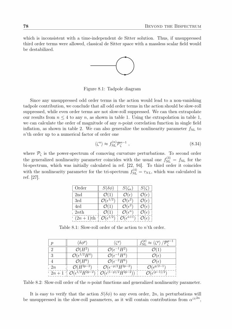
78 Beyond the Bispectrum
which is inconsistent with a time-independent de Sitter solution. Thus, if unsuppressedthird order terms were allowed, classical de Sitter space with a massless scalar field wouldbe destabilized.
Figure 8.1: Tadpole diagram
Since any unsuppressed odd order terms in the action would lead to a non-vanishingtadpole contribution, we conclude that all odd order terms in the action should be slow-rollsuppressed, while even order terms are not slow-roll suppressed. We can then extrapolateour results from n ≤ 4 to any n, as shown in table 1. Using the extrapolation in table 1,we can calculate the order of magnitude of any n-point correlation function in single fieldinflation, as shown in table 2. We can also generalize the nonlinearity parameter fNL ton’th order up to a numerical factor of order one
〈ζn〉 ≈ f(n)NLP
n−1ζ , (8.34)
where Pζ is the power-spectrum of comoving curvature perturbations. To second orderthe generalized nonlinearity parameter coincides with the usual one f (3)
NL = fNL for thebi-spectrum, which was initially calculated in ref. [22, 94]. To third order it coincideswith the nonlinearity parameter for the tri-spectrum f
(4)NL = τNL, which was calculated in
ref. [27].
Order S(δφ) S(ζn) S(ζ)
2nd O(1) O(ε) O(ε)
3rd O(ε1/2) O(ε2) O(ε)4rd O(1) O(ε2) O(ε)2nth O(1) O(εn) O(ε)
(2n+ 1)th O(ε1/2) O(εn+1) O(ε)
Table 8.1: Slow-roll order of the action to n’th order.
p 〈δφp〉 〈ζp〉 f(p)NL ≈ 〈ζp〉 /P
p−1ζ
2 O(H2) O(ε−1H2) O(1)
3 O(ε1/2H4) O(ε−1H4) O(ε)4 O(H6) O(ε−2H6) O(ε)
2n O(H2p−2) O(ε−p/2H2p−2) O(εp/2−1)
2n+ 1 O(ε1/2H2p−2) O(ε(1−p)/2H2p−2)) O(ε(p−1)/2)
Table 8.2: Slow-roll order of the n-point functions and generalized nonlinearity parameter.
It is easy to verify that the action S(δφ) to any even order, 2n, in perturbations willbe unsuppressed in the slow-roll parameters, as it will contain contributions from α(2)2n,

Challenges of Numerical Computation 79
which is unsuppressed in the slow-roll parameters. Similarly, to odd orders α(2) will alwaysappear in combination with some α(n) or χ(n) to odd order, say α(1) which is slow-rollsuppressed.
As an example we predict that the nonlinearity parameter related to the 5- and 6-pointfunction is f (5)
NL = f(6)NL = ε2.
Finally, let us briefly discuss what would be the effect of including gravitational wavemodes in the analysis. For gravitational waves the discussion of the de Sitter limit is a littlemore involved. One can have unsuppressed odd n-terms in the action with gravitationalwaves, γij, of the form ∂iδφ∂jδφγ
ij, since they will not contribute to the tadpole of thescalar field fluctuation. However, terms like δφγij γij have to be slow-roll suppressed,because they will contribute to the tadpole with a graviton circulating in the loop. Thisagrees with the results of ref. [22], where the third order action including gravitationalwaves has been calculated.
8.4 CHALLENGES OF NUMERICAL COMPUTATION
When one tries to repeat the approach of chapter 5 to calculate the trispectrum numer-ically, one is faced with an enormous complication in the sheer number of terms neededto be calculated when computing the four-point function from the action in eq. 8.26 onpage 76. One can certainly do a fair approximation for fast roll models by only extractingthe terms, that contain derivatives of the second slow roll parameter ηH , but this wouldonly be a reasonable description right at the fast roll feature in the potential.
Even if one writes down all the terms for calculation, one has to contemplate the wayone represents the quadrangle formed by the momenta of the four-point function. As itturns out it is no longer sufficient to describe the momenta by their lengths once one gobeyond the bispectrum.
Regarding n vectors in a D-dimensional momentum space, one has, at first glance,Dn degrees of freedom (DOF). The requirement of momentum conservation discards D ofthese DOF. The further requirement of isotropy makes it possible to rotate the structurein a suitable way, removing D − 1 DOF from the first vector, D − 2 from the second andso forth. This leaves
DOF = D(n− 1)− D(D − 1)
2+
max(0, D − n) [max(0, D − n) + 1]
2(8.35)
for n ≥ 2. For four vectors in three dimensions this implies that one needs six parametersto describe the quadrangle.
One realisation of this could be the size of the four momenta, the length of the twodiagonals (α and β). See figure 8.2 on the following page. These additional DOF addsa plethora of signature configurations, extending far beyond the three of the momentumtriangle. Regarding the quadrangle as two triangles, one can apply the ideas of the threetypes of triangles to the quadrangle to get a handle of the types. Some of these werediscussed in chapter 5. Among these are the squeezed limits k1 = k2 = k3 k4 andk1 = k2 k3 k4, as well as the counter-collinear limit. This last can be expressedhaving one of the diagonals going to zero.
Finally one can imagine special cases inspired by definition of τNL (eq. 3.43 on page 29).The equivalent case of the equilateral triangle would be a rhombus twisted in three dimen-sions, defined by k1 = k2 = k3 = k4 = k. Such a configuration reduces the the number of

80 Beyond the Bispectrum
Figure 8.2: Momentum quadrangle parameterized in terms of the lengths and diagonals
terms in the definition of τNL to two as only the diagonals α and β differ. Another optionwould be to keep the diagonals equal (α = β) reducing the number of terms to six. Aconfiguration where the momenta are pair wise orthogonal would reduce the number ofterms in the integral, but besides from that such a configuration would not offer any formof simplification.
The combination of the former two cases with k1 = k2 = k3 = k4 = α = β = k, forminga regular tetrahedron, reduces all the inner product between momenta to
ki · kj = ±kikj2
, (8.36)
reducing complexity of the integrals greatly (see further eq. 8.26 on page 76)It could be interesting to categorise which quadrangle shapes give a large trispectrum,
much like the discussion of triangle shapes and the bispectrum at the end of chapter 4.

9 CONCLUDING REMARKS
As inflation is about to enter its fourth decade as a cosmological theory, it has nes-tled itself firmly as the prominent description of the primordial dynamic of the Universe.Though other scenarios are present [95, 96], inflation is still the preferred choice in theliterature. That is not to say, that inflation is without issues at the moment. One stillneeds to get a detection of a signal that cannot be generated in any other plausible scenariothan inflation. A detection of a tensor-to-scalar ratio, and perhaps a non-Gaussian signal,would firmly settle inflation as a great model for the primordial universe, and might evengive hint of which direction one should take the search for a theory of inflation. At themoment the success of inflation rests on its simplicity and the ability to solve the FlatnessProblem and the Horizon Problem (see chapter 2), as well as producing the nearly scaleinvariant power spectrum in a very generic way (see chapter 4).
Even if one imagines that the Planck satellite do detect a tell tale signal for inflation,many questions concerning the early universe still need to be resolved. One still has tosettle the matters of initiating and ending inflation (discussed towards the end of chapter1). To trigger the onset of inflation, one needs to deplete the inflaton of its kinetic energyand remain in slow roll for the duration of inflation. Secondly the initial patch thatinflates to become our universe may contain initial inhomogeneities that could hinder theaccelerated expansion (see e.g. [71, 97] for a further discussion). The matter of endinginflation seems slightly more concrete as it often happens at energies where the currenttheories are more justified. There is, however, still a large task ahead for anyone trying towork out the exact details of what goes on, when inflation ends. The solution of these twoproblems is essential for gaining a complete understanding of inflation and testing whetheror not it is the correct scenario for the early universe.
Since its emergence in 1981 [14], inflation has matured as a concept. The focus hasshifted from merely achieving and sustaining inflation to investigating the perturbationscreated by the inflaton. Concentrating on creating the required primordial spectrum,models became more elaborate and the body of inflationary models seemed to expandinsatiably [37, 38]. Today many of these models have been investigated beyond lowestorder. Many types have been classified depending on the kind and amount of non-Gaussiansignature they produce.
One such model was investigated in chapter 5. This model, the axion monodromymodel, comes from a certain realisation of string theory. The model produces a distinctoscillation in both the power spectrum and the bispectrum, but where the oscillations inthe power spectrum is below the detection limit, one would clearly see the signature in thefNL with measurements by the Planck satellite. As part of the axion monodromy work, a

82 Concluding Remarks
code was developed by Troels Haugbølle to numerically calculate the three-point functionfor inflationary models with a single scalar field. From the simulations it was seen thatthis model is capable of producing a value of fNL that could be detected with Planck.Furthermore we derived an empirical formula for the shape of fNL for isosceles triangles.This result was later confirmed by the general derivation of the three-point function forthe axion monodromy model in [70].
With the increasing quality of observations one should strive to go beyond simplycomputing the temperature anisotropy bispectrum, and through that fNL, and computeboth the trispectrum and the remaining bispectra. The increasing observational sensitivitytranslates into an added constraint on the power spectrum and trispectrum. To calculatethis in single scalar field models, one needs the fourth order action, which was calculatedand discussed in chapter 8. This action, along with the accompanying gauge transforma-tion, is necessary to distinguish between models once a detection of fNL has been made.It is possible to produce many different models, that will give the same bispectrum (muchlike the degeneracy seen with the power spectrum), but each time one adds new type ofobserved spectrum, the reins are pulled tighter limiting the possibilities within the possiblemodels. Finally it was explained in chapter 8, why one would expect that any even orderof the action for field perturbations is not suppressed by slow roll parameters. This arisesfrom the fact that these terms do not contribute to the tadpole’s expectation value, whichmust vanish in the de Sitter limit.
Comparing a calculated primordial fNL to the observed one is by no means an easyfeat. One could easily have the impression that once the cumbersome task of calculatinga primordial fNL is finished, the process of evolving the result from the end of inflationto present time is straight forward. This is, however, not the case and the computationwill, in fact, involve integrals that are numerically difficult to carry out. This was thetopic of chapter 7, which summarises a work in progress. Here we developed a recursionscheme for calculating the integral over the spherical Bessel functions, and in that wayavoid having to perform a difficult numerical computation. The method was demonstratedon the two triangles with l1 + l2 + l3 = 4. These triangles, (1, 1, 2) and (0, 2, 2), are the firstnon-trivial triangles one encounters when using the recursive scheme. This demonstrationshowed that the calculated integrals were well defined for both the squeezed and flattenedlimits. One would expect that this would hold true for any triangle, but that was onlyshowed, in part, for the triangles of the type (0, l, l). At the time of writing, we still needto completely debug and optimise the code for computing the remaining integrals.
In a time where we are on the verge of obtaining what could be the first positive de-tection of fNL and quite possibly the shape of it, it is alluring to believe, that it is only amatter of time before one finds the correct model of inflation. One should, however, re-member that many models will be able to produce the same signatures, and reconstructingthe potential from observations seems discouraging as the inflaton only tracks a small partof the potential during inflation [98, 99, 100]. Though this complicates matters greatly, itdoes not make the quest futile.
Instead of seeing inflation as the one and only tool for making inference on high energyphysics, it should stand as one test among many that any theory of high energy physicsmust face. In this sense cosmology, and especially inflation, is a great laboratory capableof probing energy ranges that we cannot probe here on Earth. This comes, of course,at the cost of having a considerable less controlled environment and very little to say inthe timing of experiments, but history has showed that with audacious study and great

83
patience these are complications, that we can overcome. Cosmology has emerged as, andwill most likely remain, a prolific source for generating and answering the fundamentalquestions of nature.
There were so many fewer questions,When stars were still just the holes to Heaven
- Jack Johnson

84 Concluding Remarks
ACKNOWLEDGEMENTS
Though these 80-odd pages have been compiled in a few months, they are a the resultof four years of work and many more years of living and dreaming. The thesis from coverto cover holds a road map of the paths my life has taken over the last years, a string ofmemories both good and bad. As one traverses such a landscape of experiences a lot ofgratitude accumulates. Mentioning all that deserves a word would double the length ofthis work, and I will therefore try to limit the specifics.
First of all I would like to thank my supervisor Steen Hannestad, who have guidedme through the last four years with a philosophy, that allowed me the freedom to explorethe ideas, that I found interesting, but at the same time always seemed to be there withcareful advice, when it was called for. Under Steen’s supervision I have certainly learnedto be more independent. This was a lesson he taught me from day one, when he left mein the care of a local television news crew for an afternoon of interviews at selected sitesin Aarhus. The next day his only comment was: "I knew you could handle it, and you didfine".
As my second supervisor Martin S. Sloth still stands as the one, who got me involvedwith inflation and those maddening long equations. This turned out to be an interestingprocess of calculating, recalculating and rethinking, interspersed with trips to Martin’soffice for yet another discussion on the workings of the Universe. Still it produced twoarticles that I feel good about having my name on, and through Martin’s help I learnedmany important lessons on Life, The Universe and Everything.
The last of the collaborators, Troels Haugbølle, has been a guide deeper into numer-ical physics. An always patient sparring partner who could both listen, explain and argue,Troels is the source of much of my understanding of the practicalities of inflation. I amgoing to miss the days of debugging, plotting and writing, followed by late night Thai.
Tina Lund has always been prepared to commit fully to lifting the process and theresult to a higher level. Whether it was the case of physics, relaxation, adventure or simplymy mistreatment of the English language (in this thesis amongst other), Tina has alwaysweighed in with sound suggestions, that often turned out to be the best solution. She hasthe ability to put a smile on my face and tell me to just keep swimming.
It is remarkable when you on those rare occasions meet someone, who possesses a vastknowledge and keen insight into a science, while at the same time is able to communicateit in a thoughtful and logical way, without coming off as superior or intimidating. JanHamann has for me always been such a person. It has been a great joy to discuss withhim and learn from him, all the while enjoying his good-natured approach to life, as wellas sharing his lust for ice cream. The fact that he took the time to comment on this workhas given me great reassurance.

86 Acknowledgements
My first day at University of Aarhus brought more than television cameras. It wasthe same day, that I met a man who would follow me from first to last of this Ph.D.Jacob Brandbyge has been a firm part of my everyday for the last four years and hehas always been ready with a patient ear, when the rambling overtook me. Always calm,knowledgeable and with a eye on the world with all its sports and politics, Jacob has beena great source of inspiration whenever the world drifted from my awareness. I guess it istime to leave this place and buy that BMW.
I have over the years enjoyed many great moments with the entire CAPPA group,both those mentioned above and the rest of the group. Anders Basbøll, Ole Bjælde, AnnaSejersen Riis, Katrine Skovbo and Thomas Tram Bülow have all been part of brighteninganything from a coffee break to a late night at the pub. I will miss looking at themapologetic after a fun evening and say: "I have to catch the next train back home, so....".
A constant through my work on inflation has been the asteroseismology people thatat all times have reminded me, in good spirit, that one should have data to do astrophysics.I am still not quite sure, that I believe them. I suppose the first chapter is partly in theirhonour. It is as close to data as I will ever get!
Finally, life is much more than work and career. Though too many to be mentionedby name, my deepest gratitude belongs to family, friends and loved ones, who havealways been there to hold me close or kick me around, to drag me to safe ground or followme off the deep end, to do what was necessary. Without you I would not have made itthrough these last four years, let alone this far.

BIBLIOGRAPHY
[1] James B. Hartle. Gravity - An Introduction to Einstein’s General Relativity. AddisonWesley, 1. edition, 2003.
[2] Barbara Ryden. Introduction to Cosmology. Addison Wesley, 1. edition, 2003.
[3] Douglas Clowe et al. A direct empirical proof of the existence of dark matter.Astrophys. J., 648:L109–L113, 2006, astro-ph/0608407.
[4] T. S. van Albada, John N. Bahcall, K. Begeman, and R. Sancisi. THE DISTRIBU-TION OF DARK MATTER IN THE SPIRAL GALAXY NGC- 3198. Astrophys.J., 295:305–313, 1985.
[5] D. J. Fixsen et al. The Cosmic Microwave Background Spectrum from the FullCOBE/FIRAS Data Set. Astrophys. J., 473:576, 1996, astro-ph/9605054.
[6] WMAP Homepage. http://map.gsfc.nasa.gov/. July 18, 2010.
[7] P. J. E. Peebles and Bharat Ratra. The cosmological constant and dark energy. Rev.Mod. Phys., 75:559–606, 2003, astro-ph/0207347.
[8] E. Komatsu et al. Five-Year Wilkinson Microwave Anisotropy Probe (WMAP) Ob-servations:Cosmological Interpretation. 2008, 0803.0547.
[9] M. Kowalski et al. Improved Cosmological Constraints from New, Old and CombinedSupernova Datasets. Astrophys. J., 686:749–778, 2008, 0804.4142.
[10] Daniel J. Eisenstein et al. Detection of the Baryon Acoustic Peak in the Large-ScaleCorrelation Function of SDSS Luminous Red Galaxies. Astrophys. J., 633:560–574,2005, astro-ph/0501171.
[11] Antonio Riotto. Inflation and the theory of cosmological perturbations. 2002, hep-ph/0210162.
[12] C. P. Burgess. Lectures on Cosmic Inflation and its Potential Stringy Realizations.PoS, P2GC:008, 2006, 0708.2865.
[13] NedWright’s Cosmological Tutorial. http://www.astro.ucla.edu/∼wright/cosmo_03.htm.July 19, 2010.

88 Bibliography
[14] Alan H. Guth. The Inflationary Universe: A Possible Solution to the Horizon andFlatness Problems. Phys. Rev., D23:347–356, 1981.
[15] Lev Kofman, Andrei D. Linde, and Alexei A. Starobinsky. Reheating after inflation.Phys. Rev. Lett., 73:3195–3198, 1994, hep-th/9405187.
[16] Matthew Colless et al. The 2dF Galaxy Redshift Survey: Spectra and redshifts.Mon. Not. Roy. Astron. Soc., 328:1039, 2001, astro-ph/0106498.
[17] Donald G. York et al. The Sloan Digital Sky Survey: technical summary. Astron.J., 120:1579–1587, 2000, astro-ph/0006396.
[18] Millennium Simulation MPA Garching. http://www.mpa-garching.mpg.de/millennium/. July 16, 2010.
[19] Hideo Kodama and Misao Sasaki. Cosmological Perturbation Theory. Prog. Theor.Phys. Suppl., 78:1–166, 1984.
[20] James M. Bardeen. Gauge Invariant Cosmological Perturbations. Phys. Rev.,D22:1882–1905, 1980.
[21] James M. Bardeen, Paul J. Steinhardt, and Michael S. Turner. Spontaneous Creationof Almost Scale - Free Density Perturbations in an Inflationary Universe. Phys. Rev.,D28:679, 1983.
[22] Juan Martin Maldacena. Non-Gaussian features of primordial fluctuations in singlefield inflationary models. JHEP, 05:013, 2003, astro-ph/0210603.
[23] Amit P. S. Yadav and Benjamin D. Wandelt. Evidence of Primordial Non-Gaussianity (fNL) in the Wilkinson Microwave Anisotropy Probe 3-Year Data at2.8σ. Phys. Rev. Lett., 100:181301, 2008, 0712.1148.
[24] Kendrick M. Smith, Leonardo Senatore, and Matias Zaldarriaga. Optimal limits onf localNL from WMAP 5-year data. JCAP, 0909:006, 2009, 0901.2572.
[25] Oystein Rudjord et al. An Estimate of the Primordial Non-Gaussianity ParameterfNL Using the Needlet Bispectrum from WMAP. Astrophys. J., 701:369–376, 2009,0901.3154.
[26] A. Curto, E. Martinez-Gonzalez, and R. B. Barreiro. Improved constraints on pri-mordial non-Gaussianity for the Wilkinson Microwave Anisotropy Probe 5-yr data.Astrophys. J., 706:399–403, 2009, 0902.1523.
[27] David Seery, James E. Lidsey, and Martin S. Sloth. The inflationary trispectrum.JCAP, 0701:027, 2007, astro-ph/0610210.
[28] Laila Alabidi and David H. Lyth. Inflation models and observation. JCAP, 0605:016,2006, astro-ph/0510441.
[29] Lotfi Boubekeur and David. H. Lyth. Detecting a small perturbation through itsnon- Gaussianity. Phys. Rev., D73:021301, 2006, astro-ph/0504046.

89
[30] David H. Lyth and Yeinzon Rodriguez. The inflationary prediction for primordialnon- gaussianity. Phys. Rev. Lett., 95:121302, 2005, astro-ph/0504045.
[31] Kendrick M. Smith and Matias Zaldarriaga. Algorithms for bispectra: forecasting,optimal analysis, and simulation. 2006, astro-ph/0612571.
[32] Eiichiro Komatsu and David N. Spergel. Acoustic signatures in the primary mi-crowave background bispectrum. Phys. Rev., D63:063002, 2001, astro-ph/0005036.
[33] Nima Arkani-Hamed, Hsin-Chia Cheng, Paolo Creminelli, and Lisa Randall. Ex-tranatural inflation. Phys. Rev. Lett., 90:221302, 2003, hep-th/0301218.
[34] Katherine Freese, Joshua A. Frieman, and Angela V. Olinto. Natural inflation withpseudo - Nambu-Goldstone bosons. Phys. Rev. Lett., 65:3233–3236, 1990.
[35] Jaume Garriga and Viatcheslav F. Mukhanov. Perturbations in k-inflation. Phys.Lett., B458:219–225, 1999, hep-th/9904176.
[36] Mohsen Alishahiha, Eva Silverstein, and David Tong. DBI in the sky. Phys. Rev.,D70:123505, 2004, hep-th/0404084.
[37] David H. Lyth and Antonio Riotto. Particle physics models of inflation and thecosmological density perturbation. Phys. Rept., 314:1–146, 1999, hep-ph/9807278.
[38] Scott Dodelson, William H. Kinney, and Edward W. Kolb. Cosmic microwavebackground measurements can discriminate among inflation models. Phys. Rev.,D56:3207–3215, 1997, astro-ph/9702166.
[39] Hans Stephani. Relativity. Cambridge University Press, 3 edition, 2004.
[40] Richard L. Arnowitt, Stanley Deser, and Charles W. Misner. The dynamics ofgeneral relativity. 1962, gr-qc/0405109.
[41] E. Komatsu et al. Non-Gaussianity as a Probe of the Physics of the PrimordialUniverse and the Astrophysics of the Low Redshift Universe. 2009, 0902.4759.
[42] Andrei D. Linde and Viatcheslav F. Mukhanov. Nongaussian isocurvature pertur-bations from inflation. Phys. Rev., D56:535–539, 1997, astro-ph/9610219.
[43] David Langlois, Filippo Vernizzi, and David Wands. Non-linear isocurvature pertur-bations and non- Gaussianities. JCAP, 0812:004, 2008, 0809.4646.
[44] David Langlois. Correlated adiabatic and isocurvature perturbations from doubleinflation. Phys. Rev., D59:123512, 1999, astro-ph/9906080.
[45] G. I. Rigopoulos, E. P. S. Shellard, and B. J. W. van Tent. Large non-Gaussianityin multiple-field inflation. Phys. Rev., D73:083522, 2006, astro-ph/0506704.
[46] N. Bartolo, S. Matarrese, and A. Riotto. On non-Gaussianity in the curvaton sce-nario. Phys. Rev., D69:043503, 2004, hep-ph/0309033.
[47] David H. Lyth, Carlo Ungarelli, and David Wands. The primordial density pertur-bation in the curvaton scenario. Phys. Rev., D67:023503, 2003, astro-ph/0208055.

90 Bibliography
[48] David H. Lyth and David Wands. Generating the curvature perturbation withoutan inflaton. Phys. Lett., B524:5–14, 2002, hep-ph/0110002.
[49] Martin S. Sloth. Superhorizon curvaton amplitude in inflation and pre-big bangcosmology. Nucl. Phys., B656:239–251, 2003, hep-ph/0208241.
[50] Xingang Chen, Richard Easther, and Eugene A. Lim. Generation and Characteri-zation of Large Non-Gaussianities in Single Field Inflation. JCAP, 0804:010, 2008,0801.3295.
[51] Xingang Chen, Richard Easther, and Eugene A. Lim. Large non-Gaussianities insingle field inflation. JCAP, 0706:023, 2007, astro-ph/0611645.
[52] Eva Silverstein and Alexander Westphal. Monodromy in the CMB: Gravity Wavesand String Inflation. Phys. Rev., D78:106003, 2008, 0803.3085.
[53] Alexei A. Starobinsky. Spectrum of adiabatic perturbations in the universe whenthere are singularities in the inflation potential. JETP Lett., 55:489–494, 1992.
[54] T. S. Bunch and P. C. W. Davies. Quantum Field Theory in de Sitter Space:Renormalization by Point Splitting. Proc. Roy. Soc. Lond., A360:117–134, 1978.
[55] Brian R. Greene, Koenraad Schalm, Gary Shiu, and Jan Pieter van der Schaar.Decoupling in an expanding universe: Backreaction barely constrains short distanceeffects in the CMB. JCAP, 0502:001, 2005, hep-th/0411217.
[56] Koenraad Schalm, Gary Shiu, and Jan Pieter van der Schaar. Decoupling in anexpanding universe: Boundary RG-flow affects initial conditions for inflation. JHEP,04:076, 2004, hep-th/0401164.
[57] F. Nitti, M. Porrati, and J. W. Rombouts. Naturalness in cosmological initial con-ditions. Phys. Rev., D72:063503, 2005, hep-th/0503247.
[58] Daniel Babich, Paolo Creminelli, and Matias Zaldarriaga. The shape of non-Gaussianities. JCAP, 0408:009, 2004, astro-ph/0405356.
[59] Xingang Chen, Min-xin Huang, Shamit Kachru, and Gary Shiu. Observationalsignatures and non-Gaussianities of general single field inflation. JCAP, 0701:002,2007, hep-th/0605045.
[60] R. Holman and Andrew J. Tolley. Enhanced Non-Gaussianity from Excited InitialStates. JCAP, 0805:001, 2008, 0710.1302.
[61] David Langlois, Sebastien Renaux-Petel, Daniele A. Steer, and Takahiro Tanaka.Primordial perturbations and non-Gaussianities in DBI and general multi-field in-flation. Phys. Rev., D78:063523, 2008, 0806.0336.
[62] Liam McAllister, Eva Silverstein, and Alexander Westphal. Gravity Waves andLinear Inflation from Axion Monodromy. 2008, 0808.0706.
[63] Steen Hannestad, Troels Haugbolle, Philip R. Jarnhus, and Martin S. Sloth. Non-Gaussianity from Axion Monodromy Inflation. JCAP, 1006:001, 2010, 0912.3527.

91
[64] Raphael Flauger, Liam McAllister, Enrico Pajer, Alexander Westphal, and GangXu. Oscillations in the CMB from Axion Monodromy Inflation. 2009, 0907.2916.
[65] Paolo Creminelli and Matias Zaldarriaga. Single field consistency relation for the3-point function. JCAP, 0410:006, 2004, astro-ph/0407059.
[66] Xingang Chen, Min-xin Huang, and Gary Shiu. The inflationary trispectrum formodels with large non- Gaussianities. Phys. Rev., D74:121301, 2006, hep-th/0610235.
[67] David Seery, Martin S. Sloth, and Filippo Vernizzi. Inflationary trispectrum fromgraviton exchange. JCAP, 0903:018, 2009, 0811.3934.
[68] Noriyuki Kogo and Eiichiro Komatsu. Angular Trispectrum of CMB TemperatureAnisotropy from Primordial Non-Gaussianity with the Full Radiation Transfer Func-tion. Phys. Rev., D73:083007, 2006, astro-ph/0602099.
[69] Jan Hamann, Steen Hannestad, Martin S. Sloth, and Yvonne Y. Y. Wong. Observingtrans-Planckian ripples in the primordial power spectrum with future large scalestructure probes. JCAP, 0809:015, 2008, 0807.4528.
[70] Raphael Flauger and Enrico Pajer. Resonant Non-Gaussianity. 2010, 1002.0833.
[71] Daniel Baumann. TASI Lectures on Inflation. 2009, 0907.5424.
[72] Chung-Pei Ma and Edmund Bertschinger. Cosmological perturbation theory in thesynchronous and conformal Newtonian gauges. Astrophys. J., 455:7–25, 1995, astro-ph/9506072.
[73] Scott Dodelson. Modern Cosmology. Academic Press, 1 edition, March 2003.
[74] M. R. Nolta et al. Five-Year Wilkinson Microwave Anisotropy Probe (WMAP)Observations: Angular Power Spectra. Astrophys. J. Suppl., 180:296–305, 2009,0803.0593.
[75] Daniel Baumann et al. CMBPol Mission Concept Study: Probing Inflation withCMB Polarization. AIP Conf. Proc., 1141:10–120, 2009, 0811.3919.
[76] Matias Zaldarriaga and Uros Seljak. An All-Sky Analysis of Polarization in theMicrowave Background. Phys. Rev., D55:1830–1840, 1997, astro-ph/9609170.
[77] Marc Kamionkowski, Arthur Kosowsky, and Albert Stebbins. Statistics of Cos-mic Microwave Background Polarization. Phys. Rev., D55:7368–7388, 1997, astro-ph/9611125.
[78] Thibault Damour and Alexander Vilenkin. Gravitational wave bursts from cuspsand kinks on cosmic strings. Phys. Rev., D64:064008, 2001, gr-qc/0104026.
[79] Levon Pogosian, Mark C. Wyman, and Ira Wasserman. Observational constraintson cosmic strings: Bayesian analysis in a three dimensional parameter space. JCAP,0409:008, 2004, astro-ph/0403268.

92 Bibliography
[80] P. Binetruy, A. Bohe, T. Hertog, and Daniele A. Steer. Gravitational WaveBursts from Cosmic Superstrings with Y- junctions. Phys. Rev., D80:123510, 2009,0907.4522.
[81] Katherine Jones-Smith, Lawrence M. Krauss, and Harsh Mathur. A Nearly ScaleInvariant Spectrum of Gravitational Radiation from Global Phase Transitions. Phys.Rev. Lett., 100:131302, 2008, 0712.0778.
[82] Andrew R. Liddle and D. H. Lyth. Cosmological inflation and large-scale structure.ISBN-13-9780521828499.
[83] Scott Dodelson. Coherent phase argument for inflation. AIP Conf. Proc., 689:184–196, 2003, hep-ph/0309057.
[84] David N. Spergel and Matias Zaldarriaga. CMB polarization as a direct test ofinflation. Phys. Rev. Lett., 79:2180–2183, 1997, astro-ph/9705182.
[85] James Bock et al. The Experimental Probe of Inflationary Cosmology (EPIC): AMission Concept Study for NASA’s Einstein Inflation Probe. 2008, 0805.4207.
[86] J. R. Fergusson and Edward P. S. Shellard. Primordial non-Gaussianity and theCMB bispectrum. Phys. Rev., D76:083523, 2007, astro-ph/0612713.
[87] Li-Min Wang and Marc Kamionkowski. The cosmic microwave background bispec-trum and inflation. Phys. Rev., D61:063504, 2000, astro-ph/9907431.
[88] Milton Abramowitz and Irene A. Stegun, editors. Handbook of Mathematical Func-tions With Formulas, Graphs, and Mathematical Tables. National Bureau of Stan-dards, 10 edition, 1973.
[89] Philip R. Jarnhus and Martin S. Sloth. de Sitter limit of inflation and nonlinearperturbation theory. JCAP, 0802:013, 2008, 0709.2708.
[90] Marco Bruni, Sabino Matarrese, Silvia Mollerach, and Sebastiano Sonego. Pertur-bations of spacetime: Gauge transformations and gauge invariance at second orderand beyond. Class. Quant. Grav., 14:2585–2606, 1997, gr-qc/9609040.
[91] Martin S. Sloth. On the one loop corrections to inflation and the CMB anisotropies.Nucl. Phys., B748:149–169, 2006, astro-ph/0604488.
[92] David Seery. One-loop corrections to a scalar field during inflation. JCAP, 0711:025,2007, 0707.3377.
[93] Martin S. Sloth. On the one loop corrections to inflation. II: The consistency relation.Nucl. Phys., B775:78–94, 2007, hep-th/0612138.
[94] Viviana Acquaviva, Nicola Bartolo, Sabino Matarrese, and Antonio Riotto. Second-order cosmological perturbations from inflation. Nucl. Phys., B667:119–148, 2003,astro-ph/0209156.
[95] Jean-Luc Lehners. Ekpyrotic and Cyclic Cosmology. Phys. Rept., 465:223–263, 2008,0806.1245.

93
[96] Justin Khoury, Burt A. Ovrut, Paul J. Steinhardt, and Neil Turok. The ekpy-rotic universe: Colliding branes and the origin of the hot big bang. Phys. Rev.,D64:123522, 2001, hep-th/0103239.
[97] Ram Brustein and Paul J. Steinhardt. Challenges for superstring cosmology. Phys.Lett., B302:196–201, 1993, hep-th/9212049.
[98] Kenji Kadota, Scott Dodelson, Wayne Hu, and Ewan D. Stewart. Precision of infla-ton potential reconstruction from CMB using the general slow-roll approximation.Phys. Rev., D72:023510, 2005, astro-ph/0505158.
[99] James M. Cline and Loison Hoi. Inflationary potential reconstruction for a WMAPrunning power spectrum. JCAP, 0606:007, 2006, astro-ph/0603403.
[100] Richard Easther and William H. Kinney. Monte Carlo reconstruction of the infla-tionary potential. Phys. Rev., D67:043511, 2003, astro-ph/0210345.

94 Bibliography

A APPENDIX
αφ(1) = − φ2
c
2H2ζn (A.1)
χφ(1) =
φ2c
2H2∂−2ζn (A.2)
αφ(2) =
φ4c
8H4ζ2n −
1
2H∂−2
(φcH∂i
[φcH
H2ζn −
φcHζn −
φcHζn
]∂iζn +
φ4c
4H4ζn∂
2ζn
+φcH
[φcH
H2ζn −
φcHζn −
φcHζn
]∂2ζn −
φ4c
4H4∂i∂jζn∂
i∂j∂−2ζn
)(A.3)
4H∂2χφ(2) =− φc
H2∂iζn∂
iζn − V ′′φ2c
H2ζ2n +
φ4c
4H4ζ2n −
φ4c
4H4∂i∂j∂
−2ζn∂i∂j∂−2ζn
− φ4c
H3∂i∂−2ζn∂
iζn −2φ3
c
H2
(φcH
H2− φcH
)ζ2n
− (3φ4
c
4H4ζ2n − 2αφ
(2))(−6H2 + φ2c)−
[φcH
H2ζn −
φcHζn −
φcHζn
]2
(A.4)
1
2βφi
(2) = ∂−2
(2H∂iαφ
(2) − φ4c
H3ζn∂iζn +
φcH
[φcH
H2ζn −
φcHζn −
φcHζn
]∂iζn
+φ4c
2H3ζn∂iζn +
φ4c
4H4ζn∂iζn −
φ4c
4H4∂jζn∂i∂
j∂−2ζn
) (A.5)