A Multimodel Assessment of RKW Theory’s Relevance to ... · RKW theory applies to squall-line...

A Multimodel Assessment of RKW Theory’s Relevance to Squall-Line Characteristics

GEORGE H. BRYAN AND JASON C. KNIEVEL

National Center for Atmospheric Research,* Boulder, Colorado

MATTHEW D. PARKER

Department of Marine, Earth, and Atmospheric Sciences, North Carolina State University, Raleigh, North Carolina

(Manuscript received 7 September 2005, in final form 20 December 2005)

ABSTRACT

The authors evaluate whether the structure and intensity of simulated squall lines can be explained by“RKW theory,” which most specifically addresses how density currents evolve in sheared environments. Incontrast to earlier studies, this study compares output from four numerical models, rather than from justone. All of the authors’ simulations support the qualitative application of RKW theory, whereby squall-linestructure is primarily governed by two effects: the intensity of the squall line’s surface-based cold pool, andthe low- to midlevel environmental vertical wind shear. The simulations using newly developed modelsgenerally support the theory’s quantitative application, whereby an optimal state for system structure alsooptimizes system intensity. However, there are significant systematic differences between the newer nu-merical models and the older model that was originally used to develop RKW theory. Two systematicdifferences are analyzed in detail, and causes for these differences are proposed.

1. Introduction

Many studies of numerically simulated squall linesimplicate the surface-based cold pool and environmen-tal vertical wind shear as critical factors in determininga system’s structure and evolution (e.g., Hane 1973;Thorpe et al. 1982; Nicholls et al. 1988; Fovell andOgura 1989; Szeto and Cho 1994; Fovell and Dailey1995; Robe and Emanuel 2001; Parker and Johnson2004a; James et al. 2005). An ongoing area of researchaddresses why details such as cold pool intensity andshear are important. To this end, in 1988 Rotunno et al.(1988; hereafter referred to as RKW88) and Weisman etal. (1988, hereafter referred to as WKR88) advanced atheory based on numerical simulations, theoretical rea-soning, and an observational review. Their theory—now often called “RKW theory” after the three au-

thors’ names—argues that environmental shear “funda-mentally alters” the circulation associated with adensity current (i.e., cold pool). Specifically, the shearcounteracts the cold pool’s tendency to sweep environ-mental air over the top of the cold pool. An optimalstate exists wherein the shear approximately balancesthe cold pool’s circulation, leading to the deepest liftingof environmental air.

Extending the theory to more complex squall lines,RKW88 argued that lifting at the leading edge of coldpools is an essential element in squall lines, because itgenerates new convective cells. Thus, RKW88 con-cluded that the combination of the relative effects ofcold pool intensity and environmental shear is also animportant mechanism for squall-line strength and evo-lution. The applicability of RKW theory to squall lines,rather than just to density currents in isolation, wasaddressed in a broad series of numerical simulations byRKW88 and WKR88. The authors concluded that therelative balance of cold pool intensity and shear mag-nitude was the “most significant factor” in determiningsquall-line structure, evolution, and intensity.

These conclusions were reassessed recently by Weis-man and Rotunno (2004, hereafter referred to asWR04). Their study had two parts. In the first, their

* The National Center for Atmospheric Research is sponsoredby the National Science Foundation.

Corresponding author address: George H. Bryan, National Cen-ter for Atmospheric Research, 3450 Mitchell Lane, Boulder, CO80301.E-mail: [email protected]

2772 M O N T H L Y W E A T H E R R E V I E W VOLUME 134

© 2006 American Meteorological Society

MWR3226

idealized simulations of cold pools spreading in shearedflow reconfirmed the main element of RKW theory(i.e., that “cold-pool lifting is especially enhanced bylow-level shear”; WR04, p. 363). Their simulationsdemonstrated that deepest lifting occurs when the twoprocesses (cold pool and shear) approximately balance,and when shear is confined to the cold pool depth. Theauthors also addressed a series of papers that investi-gated this problem from a different perspective (e.g.,Xu et al. 1996; Xue et al. 1997; Xue 2000a, 2002), assummarized in the first paragraph in section 2 of thepaper by WR04.

In the second part of their paper, WR04 evaluatedthe degree to which RKW theory’s cold pool–shear in-teraction could explain the structure, evolution, and in-tensity of simulated squall lines in a broad range ofenvironmental shears, including deep layers of shearand elevated layers of shear. The authors also usedlarger domains and higher resolution than were used byWKR88, and they used more quantitative measures ofsystem intensity in their analysis. WR04 concluded thattheir results reconfirmed the findings of RKW88 andWKR88 that the relative effects of the cold pool andshear can explain many aspects of squall-line structureand intensity. However, WR04 concluded (p. 380) thatone aspect of their earlier studies—system longevity—can no longer be considered a part of their argument,because all of their simulated squall lines were longlived (out to 6 h). The cause of the rapid squall-linedemise in the simulations by RKW88 and WKR88was first explained by Fovell and Ogura (1989, theirsection 5a).

From a certain perspective, RKW theory is not atheory for strong, long-lived squall lines, despite thetitles chosen by RKW88 and WR04. Most specifically,the theory addresses and explains the interaction be-tween density currents and environmental shear. Manymeteorologists, however, are interested in how wellRKW theory applies to squall-line characteristics, suchas structure and intensity.

As applied to squall-line structure, RKW theory’srelevance is summarized in conceptual figures such asWR04’s Fig. 2. That is, systems lean upshear when thecold pool is more intense than the low- to midlevelshear, and systems lean downshear when the shear ismore intense than the cold pool. The optimal state isthe condition wherein these two effects roughly bal-ance, and the system’s updrafts are approximately up-right and collocated with the surface gust front (i.e., theleading edge of the cold pool). Therefore, as discussedby WR04 (p. 381), the optimal state for squall-linestructure is simply one point in a continuum, with out-flow-dominated systems on one end, and shear-

dominated systems on the other end. The ability ofsuboptimal squall lines (from the perspective of RKWtheory) to be strong and long lived has been pointedout by many authors since RKW88, including (but notlimited to) WKR88, Fovell and Ogura (1988, 1989),Lafore and Moncrieff (1989), Rotunno et al. (1990),and Coniglio and Stensrud (2001). There is also somedebate about the exact structure of a squall line in theoptimal state, with notable conceptual models beingoffered by Fovell and Ogura (1989, their “solitary, per-sistent updraft”) and by James et al. (2005, their “sla-bular convective line”).

As applied to squall-line intensity, RKW theory’s rel-evance is not immediately obvious, because the inten-sity of lifting at the cold pool edge is not necessarilyrelated to overall system intensity. Therefore, a primarygoal of the squall-line simulations by WR04 was to ad-dress this application of the theory. WR04 showed thatsome measures of system intensity (e.g., total rainfalland surface wind speed) were enhanced in a mannerthat was consistent with RKW theory’s focus on therelative effects of cold pools and shear.

Stensrud et al. (2005) recently questioned whetherthe relative strengths of cold pools and shear have anyrelevance to squall-line structure and intensity, particu-larly in observed systems. They had several specificconcerns. Of particular interest to us, Stensrud et al.noted that some quantitative measures of system inten-sity in WR04’s results were not largest for systems thatwere near the optimal state from the perspective ofRKW theory. The authors contended that if the inten-sity of cold pool lifting is directly relevant to squall-lineintensity, there should be a peak in system intensityapproximately near the optimal state.

However, we question whether this lack of an ex-pected peak in system intensity in WR04’s results is ageneral weakness of RKW theory’s applicability tosquall-line intensity, or whether it is an artifact of thenumerical model used by WR04. That different modelsproduce different results is widely recognized in meso-scale research, and many studies have addressed theissue. For instance, several model comparisons have re-cently been conducted on deep precipitating convection(e.g., Moncrieff et al. 1997; Richardson 1999; Redel-sperger et al. 2000; Xu et al. 2002; Derbyshire et al.2004). Some of these studies used as few as two models,while others used up to eight. One of the main goals ofthese and other such studies is to identify large differ-ences in the output among different numerical models.By doing so, a model comparison can call attention tospecific model components that influence sensitivity,which then guides future model development and aidsinterpretation of output by model users.

OCTOBER 2006 B R Y A N E T A L . 2773

As an example, Redelsperger et al. (2000) analyzedresults from idealized simulations of a tropical squallline using eight numerical models. The authors foundexcellent qualitative agreement among models in termsof overall system structure and evolution. In contrast,some quantitative results such as rainfall rate differedgreatly (by more than a factor of 3). Redelsperger et al.identified three model details that were most respon-sible for differences among their simulations: the mi-crophysics parameterization, the use of two dimensions(i.e., x–z) compared to three, and the lateral boundaryconditions. They recommended that further researchshould focus on improving these aspects of numericalmodel configurations.

As far as we know, there has been no systematicevaluation of RKW theory’s relevance to squall-lineproperties that is based on a model other than that usedby RKW88 and WR04. Therefore, the main goal of ourstudy is to assess whether RKW theory’s relevance tosquall lines is supported by other numerical models.

We base our new simulations on the recent study byWR04, using the same simulation details and analysistechniques. We use three additional numerical models,all of which have been developed more recently thanthe model used by WR04. Our findings provide guid-ance for interpreting previously published results, andhave implications for ongoing model development.

2. Methodology

a. Numerical models

We present results from four numerical models inthis study. All are compressible models that use timesplitting to account for the acoustic modes (e.g., Klempand Wilhelmson 1978; Skamarock and Klemp 1994).All models use the staggered C grid (Arakawa and

Lamb 1977), and all simulations use the same physicalparameterizations, including the Kessler (1969) liquid-only microphysics scheme and the Deardorff (1980)turbulence parameterization based on a prognosticequation for turbulence kinetic energy. For three of themodels, two different model configurations are used inorder to highlight how well the models agree withthemselves in addition to how well they agree with oneanother. Thus, there are seven output members, assummarized in Table 1.

One of the members is the Klemp–Wilhelmson (KW)model. The KW model uses leapfrog-in-time integra-tion with fourth-order derivatives for horizontal advec-tion and second-order derivatives for vertical advection(Klemp and Wilhelmson 1978; Wilhelmson and Chen1982). To remove small-scale numerical noise, fourth-order artificial diffusion is used in the horizontal andsecond-order vertical diffusion acting on perturbationfields is used in the vertical. For this study, we utilizethe results from the KW model reported by WR04.

The second numerical model is version 4.5.2 of theAdvanced Regional Prediction System (ARPS) model(Xue et al. 2000). This model also uses leapfrog-in-timeintegration. For one configuration, referred to asARPS-A, the model setup is similar to that for the KWmodel. Fourth-order advection is used in all directions.Fourth-order diffusion is applied in the horizontal only.The diffusion coefficient is the default value for ARPS4.5.2, which is roughly one-half of that used by WR04.We ran additional simulations with different diffusioncoefficients and they had no influence on the main con-clusions of this paper; therefore, we present only simu-lations using the default diffusion coefficient. A newerversion of the ARPS model has a monotonic limiteravailable for high-order diffusion (Xue 2000b); thisscheme was not used herein, but Bryan (2005, p. 1993)

TABLE 1. Summary of the numerical model configurations. The information under “Advection” and “Diffusion” refers to the orderof the truncation error of the numerical scheme (when specified as second, third, etc.), or to some other detail of the formulation. Theschemes are separated by their formulation in the horizontal and vertical.

ModelAdvection

(horizontal/vertical)Diffusion

(horizontal/vertical) Other details

Comparison members:KW Fourth/second Fourth/secondARPS-A Fourth/fourth Fourth/noneARPS-B Fourth/fourth Fourth/none (u, �, w only) Scalar advection is FCT/FCTWRF-A Fifth/third Implicit, flow dependent Ck � 0.10WRF-B Fifth/third Implicit, flow dependent Ck � 0.15BF-A Fifth/fifth Implicit, flow dependentBF-B Fifth/fifth Implicit, flow dependent Scalar advection is WENO/WENO

Special simulations:BF-C Fifth/fifth Implicit, flow dependent BF-A, but without water conservationBF-D Fifth/fifth Implicit, flow dependent BF-C, but with KW vertical diffusion


found it to have little impact on simulations usingfourth-order diffusion. There is no artificial vertical dif-fusion in the ARPS-A simulations. For the second con-figuration, ARPS-B, the advection of scalars is calcu-lated by a Flux Corrected Transport (FCT) scheme(Zalesak 1979) using a fourth-order term for the high-order flux. This configuration is preferred by manyARPS users (e.g., Xue 2000a, Xue 2002), particularlyfor its ability to prevent artificial negative water values(e.g., Xue et al. 2001). The artificial diffusion of scalarsis turned off for this latter configuration. The ARPSmodel also has a positive definite advection scheme formoisture and turbulence kinetic energy [i.e., the multi-dimensional positive definite centered difference(MPDCD) scheme; Xue et al. 2001, p. 151], but we didnot use this scheme. A high-resolution two-dimensionalsimulation of a squall line that addresses aspects ofmodel design is presented in section 5 of Xue (2002).

The third numerical model is version 2.0.3.1 of theAdvanced Research core of the Weather Research andForecasting (WRF) model (Skamarock et al. 2005).This model utilizes a hydrostatic pressure vertical co-ordinate and is the only model analyzed herein thatdoes not use Cartesian height as the vertical coordinate.This version of the WRF model uses third-orderRunge–Kutta time integration (Wicker and Skamarock2002). The advection formulation for these simulationsis fifth order in the horizontal and third order in thevertical. These odd-ordered schemes are upwind biasedand contain implicit diffusion that is proportional to theadvective wind speed. No additional artificial diffusionterm is used. The two WRF model configurations usedifferent values for Ck, a parameter in the subgrid tur-bulence parameterization that is proportional to theamount of diffusion applied by this scheme (Takemiand Rotunno 2003). One configuration, WRF-A, uses atypical value, Ck � 0.10. The second configuration,WRF-B, uses Ck � 0.15, based on the recommendationof Takemi and Rotunno in their 2005 corrigendum(Takemi and Rotunno 2003).

The fourth numerical model is version 1.8 of the Bry-an–Fritsch (BF) cloud model (Bryan and Fritsch 2002).This model uses the same third-order Runge–Kuttatime integration technique as the WRF model uses. Forthese simulations, the governing equations are slightlydifferent from those in the other models; these equa-tions improve conservation of total mass and total en-ergy compared to traditional cloud model equations(Bryan and Fritsch 2002). For one configuration, BF-A,the advection scheme is fifth order in all directions, withno artificial diffusion. For the other configuration, BF-B, the advection of scalars uses the weighted essentiallynonoscillatory (WENO) scheme of Shu (2001).

In summary, there are six simulation members thatuse the relatively newly developed ARPS, WRF, andBF models. Three of the members are configured withcomparatively low diffusion, and are denoted with“-A.” The other three members, denoted with “-B,”have either increased diffusion or use nonoscillatoryadvection schemes, which are typically more diffusivethan standard, oscillatory schemes. The seventh mem-ber of the simulations is a single configuration of theKW model.

The diversity of the models in our study is rathernarrow: all use finite differences on structured grids, allare compressible and use the same time-splitting inte-gration technique, and all are configured to use thesame liquid-only microphysics scheme (Kessler 1969;Klemp and Wilhelmson 1978). Thus, the scope of theconclusions from this model comparison is limited fromthe perspective of model development. Nonetheless,these models are commonly used to study severestorms, and a comparison of their strengths and weak-nesses has merit.

b. Simulation design

The design of the numerical simulations is generallythe same as that used by WR04. The resolution, physicsschemes, and environmental conditions are constrainedby the choices made by WR04, because our study ad-dresses whether various numerical models support theconclusions of RKW88 and WR04.

One of the few ways in which our setup differs fromthat used by WR04 is the domain dimensions, which are600 km � 80 km � 20 km. The slightly deeper domain(20 km as opposed to 17.5 km used by WR04) is nec-essary to accommodate a Rayleigh damper at the top ofthe domain in the new simulations; an open radiativecondition was used by WR04. The smaller along-linedimension (80 km as opposed to 160 km used byWR04) reduces the cost of our simulations. Based on alimited set of simulations using the BF model, we findthis smaller along-line length to be sufficient for thetypes of qualitative and quantitative conclusions ad-dressed in this paper. As configured by WR04, thelonger horizontal dimension is in the across-line direc-tion, and open conditions are used at the boundaries.The shorter horizontal dimension is in the along-linedirection, and periodic boundary conditions are used.

For all of our simulations, the squall lines are initi-ated with a 1.5-K perturbation in potential temperature(�) at x � 300 km, as specified by WR04. A more in-tense perturbation was required to initiate squall lineswith the KW model in some strong shear cases (WR04,p. 369). This was not necessary with the newer numeri-cal models, with two exceptions. One is the ARPS-B


configuration with the strongest shear used herein,which eventually produces a squall line, but later thanwith all other model configurations. The second is theWRF-B configuration, also with the strongest shear,which does not produce a squall line at all. We decidedto retain these simulations rather than redo them witha stronger perturbation, because one of our goals is toreveal any systematic differences that are inherent incertain model configurations. It is useful to documentthat these two more diffusive, -B, configurations re-quire stronger forcing to initiate convection in someenvironments, as does the KW model.

In all other respects, the simulation details are thesame as those described by WR04. Small-amplitude(�0.1 K) � perturbations are inserted into the line ther-mal to initiate three-dimensional motion. The horizon-tal grid spacing is 1 km. All models use 40 verticallevels. For the height-coordinate models, this means thevertical grid spacing is constant at 500 m. For the WRFmodel, the vertical grid spacing at the initial time variesbetween 485 and 525 m. The initial thermodynamicalenvironment is horizontally homogeneous, using thesame analytic sounding as used by WR04 (Fig. 1). Allsimulations last 6 h.

In this study, we investigate only wind profiles withacross-line shear in the 0–5-km layer. Specifically, lin-ear shear is specified from 0 to 5 km, with a constantwind speed above 5 km. We refer to the simulations bythe amount of wind variation in the 0–5-km layer (�U).The along-line wind is zero.

We focus exclusively on the 0–5-km layer becausemost of WR04’s figures are from simulations with thisshear profile. We do not have access to the output fromtheir simulations, so we rely on the figures available intheir paper. WR04 did find that systems were moreintense when shear was confined to the lowest 2.5 km—the approximate depth of the cold pool—and that bowechoes were more prevalent in shallow shear. We stressthat our study does not address all aspects of RKWtheory and its applicability to squall lines, particularlybecause we focus on a narrow range of conditions.Nonetheless, we show in the next section that shearvariations in the 0–5-km layer can produce a broadrange of squall line structures, which is a key element ofour model comparison.

3. System structure

Using the KW model, WKR88 and WR04 demon-strated that an impressively broad range of systemstructures could be created by changing only low- tomidlevel shear perpendicular to the squall line. For ex-ample, in weak 0–5-km shear, simulated systems were

tilted upshear and contained mainly weak, scatteredupdrafts. In moderate 0–5-km shear, simulated systemswere nearly upright, and updrafts were more continu-ous along the line. In even stronger 0–5-km shear, sys-tems were tilted downshear, with strong, isolated cellsthat sometimes had supercellular characteristics.

These qualitative results hold for all of our simula-tions using the newer models. That is, the trend fromupshear-tilted to downshear-tilted systems with increas-ing 0–5-km shear occurs in all simulations (Figs. 2–4). Inaddition, individual updrafts tend to be weaker andsmaller in the weakly sheared environments (Fig. 5),but stronger and larger in the strongly sheared environ-ments (Fig. 6).

Among model simulations, differences in the overallsystem structure are minor. For example, when �U �10 m s�1, all models produce cold pools that are deep-est within �30 km of the surface gust front, and a cloudextends mostly upshear of the gust front (Fig. 2). When�U � 20 m s�1, the cloud at upper levels is more sym-metric, and the overall system structure is more upright(Fig. 3) than it is in weaker shear. When �U � 30 m s�1,the cloud extends mostly downshear in every case (Fig.4). For any value of �U, overall flow patterns are simi-lar among all models.

One notable difference in our study is the tendencyfor the more diffusive, -B, simulations to have slightly

FIG. 1. The initial thermodynamical sounding.


FIG. 2. Line-averaged vertical cross sections at t � 4 h for �U � 10 m s�1 from (a) ARPS-A, (b) ARPS-B, (c)WRF-A, (d) WRF-B, (e) BF-A, and (f) BF-B. System-relative flow vectors are included every 10 km horizontallyand every 500 m vertically, with a vector length of 10 km representing a vector magnitude of 15 m s�1. The 1 � 10�2

g kg�1 cloud water contour indicates the cloud boundary. Buoyancy is shaded, with light gray representing ��0.01m s�2 and dark gray representing ��0.1 m s�2.


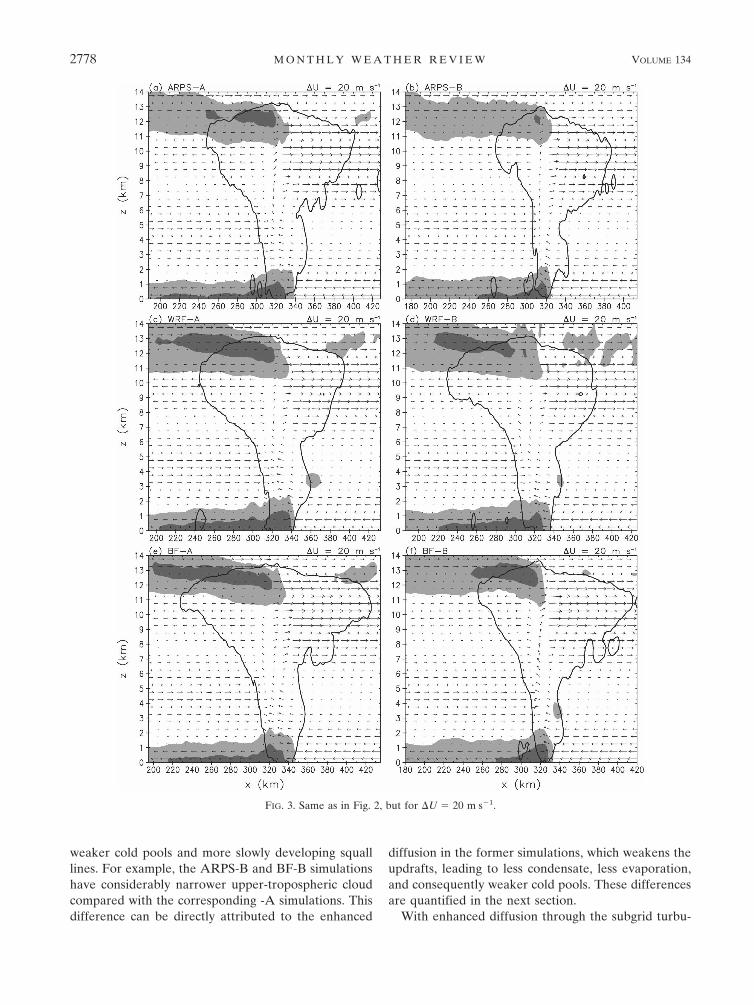
weaker cold pools and more slowly developing squalllines. For example, the ARPS-B and BF-B simulationshave considerably narrower upper-tropospheric cloudcompared with the corresponding -A simulations. Thisdifference can be directly attributed to the enhanced

diffusion in the former simulations, which weakens theupdrafts, leading to less condensate, less evaporation,and consequently weaker cold pools. These differencesare quantified in the next section.

With enhanced diffusion through the subgrid turbu-

FIG. 3. Same as in Fig. 2, but for �U � 20 m s�1.


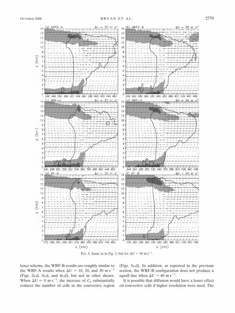
lence scheme, the WRF-B results are roughly similar tothe WRF-A results when �U � 10, 20, and 30 m s�1

(Figs. 2c,d, 3c,d, and 4c,d), but not in other shears.When �U � 0 m s�1, the increase of Ck substantiallyreduces the number of cells in the convective region

(Figs. 5c,d). In addition, as reported in the previoussection, the WRF-B configuration does not produce asquall line when �U � 40 m s�1.

It is possible that diffusion would have a lesser effecton convective cells if higher resolution were used. The

FIG. 4. Same as in Fig. 2, but for �U � 30 m s�1.


FIG. 5. Horizontal cross sections at z � 3 km and t � 4 h for �U � 0 m s�1 from (a) ARPS-A, (b) ARPS-B, (c)WRF-A, (d) WRF-B, (e) BF-A, and (f) BF-B. Positive vertical velocity is contoured every 2 m s�1. Rainwatermixing ratio is shaded, with light gray representing 1 and dark gray representing 4 g kg�1. Line-relative flowvectors are included every 4 km, with a vector length of 4 km indicating a vector magnitude of 20 m s�1. The thickdashed contour is the surface gust front.


FIG. 6. Same as in Fig. 5, but for �U � 20 m s�1. The contour interval for vertical velocity is 3 m s�1.


diffusion schemes in these models act primarily at smallscales (less than �8 times the grid spacing, or 8 kmherein). However, in our simulations the updrafts areroughly 4–8 km wide, so diffusion acts directly on them.Future studies should reevaluate the impact of diffusionand model configuration when using higher resolution,so that diffusion does not act on the scale of the con-vective updrafts.

A second notable difference among models is thetendency for the KW model to produce the deepest andstrongest cold pools. When �U � 10 m s�1, the com-parable figure from WR04 of line-averaged structure(WR04, their Fig. 12b) shows the �0.01 m s�1 buoy-ancy value at a height of 2 km at all locations west ofthe cloud boundary. In contrast, this buoyancy value isbelow 1.5 km, and typically below even 1.25 km, in allsimulations by the newer numerical models (Fig. 2).This tendency of the KW model to produce the strong-est and deepest cold pools is probably the most salientresult from this model comparison. Further details areprovided in later sections of this paper.

A third notable difference is the tendency for someof the weakly diffusive, -A, simulations to be charac-terized by an artificial updraft pattern (e.g., Figs. 5c,e).Specifically, the cells are often poorly resolved andhave a regularly repeating pattern in both the along-line and across-line directions. This pattern is especiallyprevalent when the low-level shear is weak. This is thesame problem studied with an earlier version of theWRF model by Takemi and Rotunno (2003). In a simi-lar study, Bryan (2005) argued that the pattern arisesfrom oscillatory numerics applied to flow through stati-cally unstable layers. Consequently, nonoscillatory nu-merical schemes and strong diffusion at small scalesshould be less likely to produce the pattern.

The KW model simulations produce larger updraftsand do not show evidence of an artificial organization(WR04, their Fig. 13b). We attribute this difference incellular structure to two characteristics of the KW mod-el’s diffusion schemes. First, the fourth-order horizontaldiffusion in the KW model contributes to the creationof larger cells because of the lower effective resolutionallowed by this scheme (Skamarock 2004). TheARPS-A run uses the same diffusion scheme and alsoproduces larger cells than the WRF and BF modelsproduce (e.g., Fig. 5a). The implicit diffusion in theWRF and BF models has a sixth-order form, whichpermits a higher effective resolution when a compa-rable diffusion coefficient is used (i.e., when 2� featuresare diffused at the same rate; Skamarock 2004).

A second significant attribute of the KW model con-figuration is the strong vertical diffusion acting on per-

turbation fields. In their 2005 corrigendum, Takemi andRotunno (2003) reported that vertical diffusion actingon total fields in the WRF model was more diffusiveand resulted in fewer cells, whereas diffusion acting onperturbation fields generated significantly more cellsthat were also stronger. This analysis by Takemi andRotunno (2003) is not directly relevant to the scheme inthe KW model because they addressed the formulationof the subgrid turbulence parameterization, not the sec-ond-order artificial diffusion term. Nevertheless, theirdifferences in results are significant, and may explaindifferences among our simulations, especially consider-ing that the KW model is the only configuration weused that applies vertical diffusion on perturbationfields.

A fourth notable difference among models is the ten-dency for the simulations with higher effective resolu-tion (i.e., the WRF and BF models) to produce elon-gated, plumelike updrafts in the convective region (e.g.,Figs. 5f and 6c). Houze (2004) speculated that suchstructures may be responsible for “cigar-shaped” radarechoes that are sometimes observed in the convectiveregion of mesoscale convective systems. These featureshave been studied in detail with high-resolution (�x �125 m) simulations by Bryan et al. (2006); in their simu-lations, the plumes had an average spacing of �3 km.Thus, they are poorly resolved with the 1-km grid spac-ing we used, and this might explain why they seem to bemore common with model configurations that have ahigher effective resolution.

In summary, there are some minor differences in sys-tem structure among the four models’ simulations, butthe overall qualitative structures are very similar. Thisconclusion seems to be reached in all model compari-son studies of mesoscale convective systems, and alsoholds for model comparisons that use more realisticphysical processes such as ice microphysics, surfacefluxes, and radiation (e.g., Redelsperger et al. 2000;Derbyshire et al. 2004).

Furthermore, for all of our model configurations, thetrend in system structure with increasing shear is thesame as that found by WR04. That is, updraft intensityincreases and cells become larger as low- to midlevelenvironmental shear increases (cf. Figs. 5 and 6). Thetrend from weak, upshear-tilted systems in weak shearto strong, downshear-tilted systems in strong shear isclearly captured in all simulations (Figs. 2–4). This spe-cific aspect of RKW theory’s application to squalllines—that variations in low- to midlevel shear alonecan produce a broad range of system structures, all elsebeing equal—is supported by all four numerical mod-els.


4. The optimal state

A more controversial aspect of RKW theory is theargument for an optimal state, wherein the upshear ac-celeration from the cold pool roughly balances thedownshear acceleration from the environmental shear.When approximate balance occurs, the lifting at theleading edge of the system should be the strongest anddeepest according to the theory (all else being equal).Undoubtedly, a balance can occur; however, some havequestioned whether such balance is relevant to thesquall lines’ overall characteristics.

WR04 evaluated this optimal state quantitatively viaC, a measure of cold pool intensity, and via �U, a mea-sure of shear in low to midlevels. Theoretically, theoptimal state occurs when the ratio C/�U is approxi-mately 1. One of the outstanding questions concerningRKW theory is the following: what effect does this ratiohave on other system properties, such as overall inten-sity?

WR04 showed that the value of C/�U does conformto the overall system structure predicted by the theory.Upshear-tilted structures dominate when C/�U 1,and downshear-tilted structures dominate whenC/�U � 1 (cf. Tables 1a and 1c by WR04). Hence, thereis rather convincing evidence that the ratio C/�U doeshave a strong influence on the overall structure of simu-lated squall lines, at least within the constraints ofWR04’s study.

However, this result does not directly bear on con-cerns about the relevance of the optimal state to systemintensity. To address these concerns, WR04 presentedseveral quantitative measures of system intensity, suchas wind speed at the lowest model level and total rain-fall. They noted that systems tended to be more intensewhen C/�U was close to 1. For example, as shear in lowlevels was increased, C/�U decreased from �2 to �1,and system intensity increased accordingly.

On the other hand, Stensrud et al. (2005) noted thatWR04’s quantitative measures usually did not peakwhen C/�U was about 1. In their statistical analysis ofall simulations in the WR04 study, Stensrud et al. foundthat total rainfall peaked at C/�U � 0.5, maximumupdraft at C/�U � 0.6, and average surface wind atC/�U � 1.8. Only maximum surface wind had a maxi-mum value when C/�U 1.

In this section, we evaluate the relevance of the op-timal state to measures of system intensity with our newsimulations, using the same techniques used by WR04.We do not assess the methodology of WR04, but ratherwe assess whether their conclusions are dependent onthe numerical model used for such a study.

Theoretically, C is the propagation speed of a two-

dimensional density current in an infinitely deep, un-stratified environment (Benjamin 1968),

C2 � 2�0

H

��B� dz, �1�

wherein H is the cold pool depth; B is buoyancy,

B g��

�� 0.61�q� � q�� qc � qr�; �2�

� is potential temperature; overbars indicate the mod-el’s base state, which in these simulations is the initialcondition; and q�, qc, and qr are the mixing ratios ofwater vapor, cloud water, and rainwater, respectively.We calculate C from the model output in the samemanner as WR04 did, except we use hourly output fromt � 3 to 6 h.

We define �U as the wind change in the lowest 5 km,because this is consistent with WR04. In principle, theappropriate layer to consider would be the depth of thecold pool; in fact, the simulations of idealized densitycurrents by WR04 showed that cold pool lifting wasoptimized when shear was confined to this layer. How-ever, WR04 (p. 376) provided several arguments forusing the 0–5-km layer, instead of the layer matchingthe cold pool depth. For example, they showed thatshear above the cold pool can contribute to cell gen-eration, which has also been shown by Fovell and Dai-ley (1995) and Fovell and Tan (1998).

Also following the technique of WR04, we neglectthe potentially important effect of the rear-inflow jet onthe vorticity balance at the leading edge of the system.Weisman (1992) showed how the rear-inflow jet couldbe quantitatively included in the RKW balance rela-tion. The importance of the rear-inflow jet is discussedin his paper, as well as in the papers by Lafore andMoncrieff (1989) and Fovell and Ogura (1989). How-ever, WR04 (p. 376) excluded this contribution to sys-tem structure because the ratio C/�U alone “still pro-vides a useful guide of overall system structure for awide range of shear environments.”

In the overall design of the simulations, �U is theonly parameter that is varied from one run to the next.Studies using this method often cite the �U value thatproduces the optimal condition (C/�U � 1), which werefer to as the optimal shear (�Uoptim). We also analyzethe �U that leads to maxima in certain quantitativevalues (e.g., rainfall, surface winds), which we refer toas �Umax. If �Uoptim and �Umax have similar values, itsupports the relevance of RKW theory to squall lines.

Calculations of C confirm the qualitative conclusionfrom the previous section that the KW model usuallyproduces the deepest, strongest cold pools (Fig. 7a).


FIG. 7. Quantitative output as a function of �U from the seven model configurations: (a) C, (b) C/�U, (c) total rainfall, (d) maximum(upper set of curves) and averaged (lower set) west–east winds at the lowest model level, (e) total condensation, and (f) maximumvertical velocity. The cyan horizontal line in (b) denotes C/�U � 1. In (c) and (e), the values from the ARPS, WRF, and BF modelshave been multiplied by 2 to account for the different domain sizes compared to the simulations with the KW model.


Fig 7 live 4/C

The only exception is in weak shears, for which the KWmodel results are similar to the �A model configura-tions. The average �Umax for C is 14 m s�1 with thenewer models, but is 20 m s�1 with the KW model(Table 2). In fact, there is a sharp increase in C withthe KW model between 15 and 20 m s�1; a similar fea-ture does not occur with any other numerical model(Fig. 7a).

More relevant to RKW theory is the ratio C/�U.When plotted as a function of �U, it is apparent thatthe KW model produces the optimal state (C/�U � 1)at a larger shear than do the other models (Fig. 7b);�Uoptim � 24 m s�1 for the KW model, whereas theaverage �Uoptim for the six other simulations is 19m s�1, which is 20% lower (Table 3). This is a key find-ing: the KW model requires a significantly strongershear to produce the optimal state. This model biasmight explain some differences between conclusionsbased on simulations by the KW model and conclusionsbased on observational studies of severe convectivewindstorms [e.g., section 4b(3) of Coniglio et al. 2004a].

For total rainfall, the KW model is again an outlier instronger shears (Fig. 7c). The KW model produces20%–50% more rainfall than any other model when�U 20 m s�1. Furthermore, the KW model rainfallpeaks at a considerably stronger shear, �Umax � 30m s�1, as opposed to an average �Umax of 18 m s�1 forthe other models (Table 2).

As WR04 did, we use wind speed at the lowest modellevel (z � 250 m) as a proxy for surface winds. (For theWRF model, wind speeds are interpolated to z � 250m). Also following WR04, we compute average surfacewinds uavg associated with each squall line, by calcu-lating the average west–east wind speed u at a loca-tion 10 km behind the surface gust front (defined as�� 1 K). The results (bottom set of curves in Fig. 7d)reveal a tendency for the KW model to produce stron-ger surface winds, especially in strong shear. All of thenewer models agree well with each other, and producesimilar results for both the �A and �B configurations.

The WRF model appears to have a slight tendency toproduce stronger surface winds, but this might be re-lated to the slightly higher vertical resolution near thesurface (�z 475 m). All of the newer models yield�Umax � 15 m s�1 for this variable, while for the KWmodel �Umax � 15 and 20 m s�1 (Table 2).

For maximum surface winds at any location and timeumax, some models produce a pronounced increasewhen �U increases from 35 to 40 m s�1 (Fig. 7d, theupper set of curves). In this highly sheared environ-ment, the simulated cells are supercellular. Technically,RKW theory only applies to quasi-linear convectivesystems, and not to lines of supercells. Accordingly,considering only the 0–30 m s�1 range to exclude thesecases, the newer models yield an average �Umax of 21m s�1 for umax, which is again lower than the result fromthe KW model (�Umax � 25 m s�1; Table 2).

Other quantitative measures analyzed by WR04 aremore ambiguous in their application to RKW theory’srelevance to squall-line intensity. Total condensationhas the most scatter of any variable we analyzed, par-ticularly in weak shear (Fig. 7e). For this variable, theKW model produces among the lowest values in weakshear, but the highest values in strong shear. The great-est differences between the KW model and newer mod-els is in �Umax for total condensation, with �Umax � 25m s�1 for the former, but an average �Umax � 8 m s�1

TABLE 3. The value of �U for which C/�U is 1 (i.e., the optimalshear, �Uoptim), derived by interpolating from data points inFig. 7b.

Model �Uoptim (m s�1)

KW 24ARPS-A 19ARPS-B 19WRF-A 21WRF-B 19BF-A 19BF-B 18Avg (excluding KW) 19

TABLE 2. The value of �U for which measures of system intensity are maximized (�Umax).

Model

�Umax

C Tot rainfall uavg umax Tot condensation wmax

KW 20 30 15 and 20 25 25 30ARPS-A 15 20 15 25 5 20ARPS-B 15 15 15 20 10 35WRF-A 15 20 15 25 5 35WRF-B 10 15 15 20 5 25BF-A 10 20 15 20 10 35BF-B 20 20 15 15 15 40Avg (excluding KW) 14 18 15 21 8 32


for the latter (Table 2). Thus, in terms of RKW theory,total condensation does not support the optimal-stateargument because �Umax for total condensation is farbelow the optimal shear value (excluding the resultsfrom the KW model). We suspect that the variability inweak shears is partly attributable to the spurious up-draft pattern discussed in the previous section. On theother hand, it is possible that the inclusion of ice mi-crophysics would change the expected result. Stronglyupshear-tilted squall lines typically have large strati-form regions, within which significant condensation canoccur, owing to the mesoscale updraft above the melt-ing level (e.g., Smull and Houze 1987); in this context,suboptimal squall lines might be expected to have moretotal condensation than more upright systems. Never-theless, this is one of the reasons why several measuresof system intensity are included in our analysis, and inthe analysis by WR04.

For maximum updraft velocity wmax, there is goodgeneral agreement between all models (Fig. 7f). In fact,wmax is the only variable we analyzed for which the KWmodel was not an outlier. The trend in this variable alsodoes not show an intensity peak near the optimal state,because �Umax is much greater than the optimal shearvalue (Table 2). Presumably, this tendency for maxi-mum updraft to increase with stronger shear is relatedto dynamical effects of updrafts in shear, as discussedby WR04.

Our broad determination is that the newer modelssupport WR04’s conclusions more than the KW modeldoes. That is, some measures of overall system intensityare greatest when the systems are approximately up-right. Furthermore, this upright structure occurs whenC/�U 1 (i.e., when the cold pool intensity approxi-mately balances the magnitude of environmentalshear). This supports WR04’s contention that C/�U hasan influence on overall system intensity.

In contrast, the squall lines simulated with the KWmodel switch from predominantly upshear to downs-hear tilted at a significantly stronger shear (20 m s�1

based on WR04’s Fig. 12, as opposed to �20 m s�1 inthe case of the other models, based on Figs. 2–3 herein).However, peak values of overall system intensity fromthe KW model simulations are not consistent with thevalue of �Uoptim, as indicated in Table 2.

Thus, there is convincing evidence here that some ofthe criticisms of RKW theory’s applicability to squalllines (e.g., Stensrud et al. 2005) are attributable to thenumerical model used by RKW88 and WR04, but notnecessarily to the theory itself. The results from newer,more accurate models with higher effective resolutionshow better consistency between theory and resultsthan the KW model used by RKW88 and WR04.

This result should not be interpreted as definitivesupport for RKW theory’s relevance to squall-linestructure and intensity. We have not addressed the con-cern that changes in squall-line characteristics might bemore attributable to �U than to C/�U (e.g., Stensrud etal. 2005). This ambiguity is a consequence of the ex-perimental design, in which �U is the only parameterthat varies. To address this concern, future studiescould hold shear fixed while systematically changingparameters that affect C (like midlevel equivalent po-tential temperature). All we can say, at this time, is thatthe newer numerical models provide better support forthe arguments of WKR88 and WR04, at least whenapplied within those authors’ constraints. Future stud-ies could also explore possible effects of ice microphys-ics, higher resolution, and variations in upper-levelshear. It is possible that systems should not be expectedto have a peak intensity when C/�U 1, especiallygiven the lack of extensive stratiform regions in theabsence of ice microphysics, and owing to the omissionof the rear-inflow jet in our assessment of the optimalcondition (e.g., Fovell and Ogura 1989; Weisman 1992).We return to these points in the conclusions section ofthis paper.

5. Systematic model differences

For idealized simulations such as these, there is no“truth” solution to compare against. However, by com-paring results from the four models, we have identifiednotable differences that, in some cases, have illumi-nated errors in model code. (These errors were cor-rected for all simulations presented herein.) A similarconclusion on the utility of model comparisons wasdrawn by Redelsperger et al. (2000). In this section, weexplore in detail some of the more notable systematicdifferences. Our goal is to identify a root cause of eachdifference, and thereby to provide guidance to modeldevelopers and users.

a. The BF model’s moisture

Although the difference is rather subtle, we find thatthe BF model tends to produce the lowest quantitativewater budget measures (total rainfall, total rainwaterevaporation, etc.). The BF model is the only model ofthe four that accounts for the specific heats of water inits governing equations. This effect usually produces10%–20% more condensation and rainfall in simula-tions that use traditional cloud model equations (Bryanand Fritsch 2002). Thus, the BF model’s tendency toproduce the least rainfall (Fig. 7c) is unexpected.

We attribute this difference to improved total water


conservation in the BF model compared to most of theother model configurations. For the BF-A configura-tion, the model uses an oscillatory advection scheme.Such schemes produce spurious “undershoots” that canresult in negative water mass. Often, numerical modelsused to simulate severe convective storms simply setnegative water values to zero, without moving waterfrom elsewhere in the domain to conserve total water.This technique, hereafter referred to as the noncon-serving technique, acts as an artificial source of water.Some studies have investigated the quantitative effectsof the nonconserving technique (e.g., Xue et al. 2001, p.154), but many model developers consider this artificialincrease in mass to be minor.

There are several methods to remedy this unphysicalsituation, including, but not necessarily limited to, thefollowing: using a nonoscillatory advection scheme(e.g., Smolarkiewicz and Grabowski 1990; Xue et al.2001); implementing a flux limiter to the advection ofmoisture to prevent the creation of negative values byadvection (e.g., Lafore et al. 1998; Xue et al. 2001);predicting a transformed mass variable that minimizesthe impact of the underprediction (e.g., Ooyama 2001);or applying schemes that borrow water from other partsof the domain to preserve total mass when filling innegative values (e.g., Cohen 2000).

For our simulations, the BF model sets negative wa-ter values to zero by moving water of the same classfrom neighboring grid points. The technique is nearlythe same as that described by Cohen (2000), and isreferred to herein as the forced-conservation tech-nique. The BF-B configuration uses a nonoscillatoryadvection scheme for moisture, which does not requirethe forced-conservation technique. Tests with the BFmodel show that simulations using the nonconservingtechnique can have 25% more condensate in the do-main than simulations that use the forced-conservationtechnique.

With one exception, our configurations of the KW,ARPS, and WRF models use the nonconserving tech-nique. This exception is the ARPS-B configuration,which uses a nonoscillatory advection scheme for mois-ture, and conserves water well. In fact, the ARPS-B hasless rainfall and condensation, on average, than anymodel except the BF model. It should be noted that theWRF model’s dynamical core conserves total water,but its Kessler microphysics code sets negative watervalues to zero.

Overall, we conclude that the water-conservingmodel configurations that we used produce systemati-cally less rainfall compared to the nonconserving con-figurations (e.g., Fig. 7c). For the nonconserving con-figurations, the artificially increased condensate ulti-

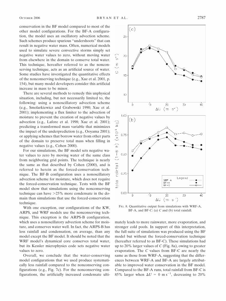
mately leads to more rainwater, more evaporation, andstronger cold pools. In support of this interpretation,the full suite of simulations was produced using the BFmodel but without the forced-conservation technique(hereafter referred to as BF-C). These simulations hadup to 20% larger values of C (Fig. 8a), owing to greaterevaporation. The C values from BF-C are nearly thesame as those from WRF-A, suggesting that the differ-ences between WRF-A and BF-A are largely attribut-able to improved water conservation in the BF model.Compared to the BF-A runs, total rainfall from BF-C is85% larger when �U � 0 m s�1, decreasing to 20%

FIG. 8. Quantitative output from simulations with WRF-A,BF-A, and BF-C: (a) C and (b) total rainfall.


larger in stronger shears (Fig. 8b). Rainfall from BF-Cis greater than that from WRF-A, possibly owing to thedifferent thermodynamical equations in the models. Ingeneral terms, these results are not necessarily surpris-ing; however, the error in total water is larger than weexpected. This highlights the need to conserve water ifquantitative precipitation values are important tomodel users.

On the other hand, as it pertains to the main focus ofthis paper, water conservation has essentially no effecton the assessment of RKW theory. When measures ofsystem intensity are compared to C/�U, the resultsfrom BF-C yield the same answers as those from BF-A.Hence, some model configurations, even though theyare unphysical, have no impact on the assessment ofRKW theory’s relevance to squall lines, at least for thismodeling methodology.

b. The KW model’s cold pools

The most conspicuous systematic difference we findamong the seven model configurations is the tendencyfor the KW model to produce deeper and more intensesurface-based cold pools, especially in stronger shears(e.g., Fig. 7a). After considering several possibilities, wefind that the formulation of the artificial vertical diffu-sion scheme in the KW model is primarily responsible.

In the KW model, artificial vertical diffusion is notapplied at the grid points closest to the bottom and topboundaries. This is equivalent to setting the flux at thesurface equal to the flux at the nearest grid point insidethe domain. Thus, the KW model can have nonzerofluxes at the top and bottom boundaries. Richardson(1999) reached the same conclusion about the verticaldiffusion scheme in a comparison between the KW andARPS models. All other model configurations that wetested have a zero-flux boundary condition at the topand bottom (in the absence of a specified heat flux orsurface drag term, which we did not include).

In the KW model, the effective boundary flux at thesurface Fsfc is

Fsfc � �K��

�z �k�1, �3�

wherein K is the diffusion coefficient, � is the variablebeing diffused, the prime indicates the deviation fromthe model’s base state, and “k � 1” refers to the firstw-level inside the domain (top or bottom) for the stag-gered vertical grid. We focus attention at the bottomboundary for the remaining analysis, because this iswhere the cold pool resides.

In the environment ahead of and far behind thesquall line, conditions near the surface remain approxi-

mately the same as in the initial state; in these locations,�� ≅ 0 and thus Fsfc ≅ 0. However, in the cold pool, thepotential temperature perturbation �� is negative at thelowest model level and approaches zero with height.Hence, ��/�z 0 and Fsfc � 0 for ��. For q�, the per-turbation is usually negative in the cold pool at thesurface and decreases (i.e., becomes more negative)with height, resulting in a positive flux at the lowerboundary. Thus, the cold pool experiences a net cooling(negative flux) and net moistening (positive flux) fromthe vertical diffusion scheme, compared to schemesthat set the flux at the boundaries to zero. In terms ofequivalent potential temperature �e, the cooling andmoistening can offset each other, resulting in approxi-mate �e conservation; for example, at 1000 hPa, �e willbe conserved with cooling of 1 K and moistening of 0.4g kg�1. The same boundary condition acts on horizontalwinds and often increases surface winds in the coldpool.

These surface fluxes from the KW vertical diffusionscheme do not represent a surface heat flux or dragterm. Rather, these effective fluxes are artifacts of theartificial diffusion term and the specific boundary con-dition for this term in the KW model. By eliminatingthe vertical diffusion at the lowest model level, thisimplementation ensures that mean profiles cannot bemodified by diffusion over time (e.g., Durran andKlemp 1983, p. 2344). This boundary condition is alsoconsistent with the assumption of a free-slip lowerboundary. Nevertheless, as formulated, the KW verticaldiffusion scheme can act as a source of mass (through �and q�) and momentum (through u and �).

Moreover, we believe this formulation of the verticaldiffusion term in the KW model is largely responsiblefor its outlying behavior. To evaluate this hypothesis,we ran a set of BF model simulations with the KWvertical diffusion scheme applied to �� and without theforced-conservation technique (BF-D), thus makingthe model more like the KW model. The resultsstrongly support our interpretation. The KW modelvertical diffusion scheme clearly increases a cold pool’sintensity (Fig. 9a), primarily by increasing its depth.Compared to the original BF-A configuration, theBF-D runs yield similar C values in weak shears, butsystematically larger C values in strong shears, muchlike the results from the KW model (Fig. 9a). In addi-tion, the value of �Uoptim from BF-D is 23 m s�1, whichis also similar to the value from the KW model (24m s�1). Furthermore, with BF-D, total rainfall increaseseven when �U �Uoptim, similar to the trend from theKW model (Fig. 9b).

These results suggest that the vertical diffusionscheme is probably responsible for the different physi-


cal response in the KW model when C/�U is less than1. Regardless of the reason, evidence points to a differ-ent numerical configuration in the KW model, and cor-responding anomalous behavior compared with theother models.

6. Conclusions

a. Summary

Several noteworthy results have emerged from thismodel comparison. First, we find model comparisons

such as this to be useful for illuminating significant dif-ferences in model configurations. In some cases, thedifferences have pointed our attention to coding errorsthat were not obvious before this study. In contrast tothe common practice of using one type of simulation,we recommend that model comparisons should explorea broad physical parameter space, such as environmen-tal shear or thermodynamics. Some differences amongthe four models in this study were only apparent whenresults were viewed as a function of shear. For example,anomalous characteristics in the KW model’s cold pooland rainfall are not apparent in weak shears, but be-come obvious when a broad range of shears are simu-lated.

Second, for these idealized simulations, we see gen-eral support for the relevance of RKW theory to squalllines. In terms of system structure, all models lead us tothe same qualitative conclusion about changes in shear,with all else being held constant: simulated squall lineshave smaller, weaker cells and are tilted upshear inweak 0–5-km shear (with C/�U 1), and have larger,stronger cells and are tilted downshear in strong 0–5-km shear (with C/�U � 1). Systems are upright andapproximately symmetric at upper levels when C/�U 1.

Third, our simulations support the argument that sys-tem intensity peaks near the optimal state, at least ac-cording to some variables, such as rainfall and near-surface winds. For our experimental design, only �Uwas varied, and the optimal state occurs when �U isslightly less than 20 m s�1 for all models except for theKW model. More importantly, this is also the approxi-mate shear value that maximizes total rainfall andmaximum surface winds for all models except for theKW model. Thus, system intensity is strongest by somemeasures when C/�U 1.

Finally, we diagnosed some systematic model differ-ences uncovered during our study. Most significantly,the KW model produces the deepest and strongest coldpools, likely owing to the way vertical diffusion is for-mulated near the lower boundary, which provides asource of cooling and moistening in the simulated coldpool. Other model differences, such as artificial updraftpatterns and water conservation, have no perceptibleimpact on the assessment of RKW theory.

b. Discussion

In this paper, we addressed some concerns aboutRKW theory, such as the relevance of the optimal stateto the intensity of simulated squall lines. We found thatthis latter concern is partially attributable to the KWmodel used by WR04, but is not necessarily a short-coming of the theory itself. However, our study doesnot address all concerns expressed in the literature

FIG. 9. Quantitative output from simulations with KW, BF-A,and BF-D: (a) C and (b) total rainfall.


about RKW theory, and should not be interpreted asdefinitive validation of RKW theory’s relevance tosquall lines.

For example, one concern about RKW theory is itsapplicability in broader environmental conditions. Thesimulations of RKW88, WKR88, WR04, and our simu-lations used only one thermodynamical profile, andtherefore they yield a fairly narrow range of C at thesquall lines’ mature state. The simulations of Weisman(1992, 1993) explored a broader range of thermody-namical conditions (e.g., CAPE from 1000 to 4500 Jkg�1), but with a smaller domain and coarser resolu-tion. In principle, RKW theory should be applicable ina wide range of environments because the ratio C/�U isimportant, not the values of C or �U by themselves.

In addition, several recent studies have highlightedhow system structure and intensity can depend on shearabove the cold pool (e.g., Fovell and Dailey 1995;Parker and Johnson 2004a; Coniglio et al. 2004b). Asimilar conclusion was reached in analytical and nu-merical studies of density currents in channels by Xu etal. (1996), Xue et al. (1997), and Xue (2000a, 2002).WR04 addressed this concern by exploring deepershear profiles and elevated shear profiles in their simu-lations of nonsteady cold pools and squall lines. Nev-ertheless, the relative importance of shear at low levelsversus upper levels in determining squall-line intensityremains an active area of research.

Future studies could also test the impacts of othermodel configurations, including the effects of ice micro-physics, radiation, and higher resolution. Of particularimportance, several studies have shown that ice micro-physics are required to produce realistic circulations insimulated convective systems (e.g., Fovell and Ogura1988; Lafore and Moncrieff 1989; Yang and Houze1995; Parker and Johnson 2004b,c). The Kesslerscheme—used herein and in the simulations ofRKW88, WKR88, and WR04—specifies only liquiddrops, which have a large fall velocity (5 m s�1). Con-sequently, all hydrometeors fall close to the convectiveline, thereby preventing the formation of extensivestratiform regions. This may be more problematic instrong shears, because the hydrometeors fall ahead ofthe cold pool and interfere with system inflow (Parkerand Johnson 2004c). There seems to be no systematicevaluation of RKW theory in simulations of squall lineswith extensive stratiform regions, and this is an obviousavenue for research in the near future.

We have followed the techniques of WR04 in ourassessment of squall-line properties, mainly because wewanted to investigate whether the conclusions fromsuch a study depend on the numerical model that isused for the simulations. However, it would be valuable

for future studies to evaluate more rigorously the RKWtheory. As a specific example, a future study couldevaluate the relative role played by the rear-inflow jet,which was identified as an important component of sys-tem structure and evolution by Fovell and Ogura(1989), Lafore and Moncrieff (1989), and Weisman(1992), but which WR04 and our study neglected.

Acknowledgments. We thank Morris Weisman andRichard Rotunno for their advice and insight duringthis project; Stan Trier, Ming Xue, and Robert Fovellfor their reviews; and Yvette Richardson for sharingher comparison of simulations using the Klemp–Wilhelmson and ARPS Models. G. Bryan was sup-ported by the Advanced Study Program at NCAR, andM. Parker was supported by the NSF under GrantATM-0349069. The Mesoscale and Microscale Meteo-rology Division of NCAR provides the version of theWRF model used herein, and the Center for Analysisand Prediction of Storms at the University of Oklaho-ma provides the ARPS model. M. Parker began thisstudy when he was a faculty member at the Universityof Nebraska–Lincoln; the ARPS simulations were per-formed using the Research Computing Facility at UNL.All figures were created with the Grid Analysis andDisplay System (GrADS).

REFERENCES

Arakawa, A., and V. R. Lamb, 1977: Computational design of thebasic dynamical processes of the UCLA general circulationmodel. Methods Comput. Phys., 17, 173–265.

Benjamin, T. B., 1968: Gravity currents and related phenomenon.J. Fluid Mech., 31, 209–248.

Bryan, G. H., 2005: Spurious convective organization in simulatedsquall lines owing to moist absolutely unstable layers. Mon.Wea. Rev., 133, 1978–1997.

——, and J. M. Fritsch, 2002: A benchmark simulation for moistnonhydrostatic numerical models. Mon. Wea. Rev., 130,2917–2928.

——, R. Rotunno, and J. M. Fritsch, 2006: Roll circulations in theconvective region of a simulated squall line. J. Atmos. Sci., inpress.

Cohen, C., 2000: A quantitative investigation of entrainment anddetrainment in numerically simulated cumulonimbus clouds.J. Atmos. Sci., 57, 1657–1674.

Coniglio, M. C., and D. J. Stensrud, 2001: Simulation of a progres-sive derecho using composite initial conditions. Mon. Wea.Rev., 129, 1593–1616.

——, ——, and M. B. Richman, 2004a: An observational study ofderecho-producing convective systems. Wea. Forecasting, 19,320–337.

——, ——, and L. J. Wicker, 2004b: How upper-level shear canpromote organized convective systems. Preprints, 22d Conf.on Severe Local Storms, Hyannis, MA, Amer. Meteor. Soc.,CD-ROM, 10.5.

Deardorff, J. W., 1980: Stratocumulus-capped mixed layer derived


from a three-dimensional model. Bound.-Layer Meteor., 18,495–527.

Derbyshire, S. H., I. Beau, P. Bechtold, J.-Y. Grandpeix, J.-M.Piriou, J.-L. Redelsperger, and P. M. M. Soares, 2004: Sensi-tivity of moist convection to environmental humidity. Quart.J. Roy. Meteor. Soc., 130, 3055–3079.

Durran, D. R., and J. B. Klemp, 1983: A compressible model forthe simulation of moist mountain waves. Mon. Wea. Rev.,111, 2341–2361.

Fovell, R. G., and Y. Ogura, 1988: Numerical simulation of a mid-latitude squall line in two dimensions. J. Atmos. Sci., 45,3846–3879.

——, and ——, 1989: Effect of vertical wind shear on numericallysimulated multicell storm structure. J. Atmos. Sci., 46, 3144–3176.

——, and P. S. Dailey, 1995: The temporal behavior of numeri-cally simulated multicell-type storms. Part I: Modes of behav-ior. J. Atmos. Sci., 52, 2073–2095.

——, and P.-H. Tan, 1998: The temporal behavior of numericallysimulated multicell-type storms. Part II: The convective celllife cycle and cell regeneration. Mon. Wea. Rev., 126, 551–577.

Hane, C. E., 1973: The squall line thunderstorm: Numerical ex-perimentation. J. Atmos. Sci., 30, 1672–1690.

Houze, R. A., Jr., 2004: Mesoscale convective systems. Rev. Geo-phys., 42, RG4003, doi:10.1029/2004RG000150.

James, R. P., J. M. Fritsch, and P. M. Markowski, 2005: Environ-mental distinctions between cellular and slabular convectivelines. Mon. Wea. Rev., 133, 2669–2691.

Kessler, E., 1969: On the Distribution and Continuity of WaterSubstance in Atmospheric Circulation. Meteor. Monogr., No.32, Amer. Meteor. Soc., 84 pp.

Klemp, J. B., and R. B. Wilhelmson, 1978: The simulation ofthree-dimensional convective storm dynamics. J. Atmos. Sci.,35, 1070–1096.

Lafore, J.-P., and M. W. Moncrieff, 1989: A numerical investiga-tion of the organization and interaction of the convective andstratiform regions of tropical squall lines. J. Atmos. Sci., 46,521–544.

——, and Coauthors, 1998: The Meso-NH atmospheric simulationsystem. Part I: Adiabatic formulation and control simula-tions. Ann. Geophys., 16, 90–109.

Moncrieff, M. W., S. K. Krueger, D. Gregory, J.-L. Redelsperger,and W.-K. Tao, 1997: GEWEX Cloud System Study (GCSS)Working Group 4: Precipitating convective cloud systems.Bull. Amer. Meteor. Soc., 78, 831–845.

Nicholls, M. E., R. H. Johnson, and W. R. Cotton, 1988: The sen-sitivity of two-dimensional simulations of tropical squall linesto environmental profiles. J. Atmos. Sci., 45, 3625–3649.

Ooyama, K. V., 2001: A dynamic and thermodynamic foundationfor modeling the moist atmosphere with parameterized mi-crophysics. J. Atmos. Sci., 58, 2073–2102.

Parker, M. D., and R. H. Johnson, 2004a: Structures and dynamicsof quasi-2D mesoscale convective systems. J. Atmos. Sci., 61,545–567.

——, and ——, 2004b: Simulated convective lines with leadingprecipitation. Part I: Governing dynamics. J. Atmos. Sci., 61,1637–1655.

——, and ——, 2004c: Simulated convective lines with leadingprecipitation. Part II: Evolution and maintenance. J. Atmos.Sci., 61, 1656–1673.

Redelsperger, J.-L., and Coauthors, 2000: A GCSS model inter-comparison for a tropical squall line observed during TOGA-

COARE. I: Cloud-resolving models. Quart. J. Roy. Meteor.Soc., 126, 823–863.

Richardson, Y., 1999: The influence of horizontal variations invertical shear and low-level moisture on numerically simu-lated convective storms. Ph.D. dissertation, University ofOklahoma, 236 pp. [Available from School of Meteorology,University of Oklahoma, 100 E. Boyd, Norman, OK 73019.]

Robe, F. R., and K. A. Emanuel, 2001: The effect of vertical windshear on radiative–convective equilibrium states. J. Atmos.Sci., 58, 1427–1445.

Rotunno, R., J. B. Klemp, and M. L. Weisman, 1988: A theory forstrong, long-lived squall lines. J. Atmos. Sci., 45, 463–485.

——, ——, and ——, 1990: Comments on “A numerical investi-gation of the organization and interaction of the convectiveand stratiform regions of tropical squall lines.” J. Atmos. Sci.,47, 1031–1033.

Shu, C.-W., 2001: High order finite difference and finite volumeWENO schemes and discontinuous Galerkin methods forCFD. ICASE Rep. 2001-11, 16 pp. [Available from NASALangley Research Center, Hampton, VA 23681-2199.]

Skamarock, W. C., 2004: Evaluating mesoscale NWP models us-ing kinetic energy spectra. Mon. Wea. Rev., 132, 3019–3032.

——, and J. B. Klemp, 1994: Efficiency and accuracy of theKlemp-Wilhelmson time-splitting technique. Mon. Wea.Rev., 122, 2623–2630.

——, ——, J. Dudhia, D. O. Gill, D. M. Barker, W. Wang, and J. G.Powers, 2005: A description of the Advanced Research WRFversion 2. NCAR Tech. Note NCAR/TN-468�STR, 88 pp.

Smolarkiewicz, P. K., and W. W. Grabowski, 1990: The multidi-mensional positive definite advection transport algorithm:Nonoscillatory option. J. Comput. Phys., 86, 355–375.

Smull, B. F., and R. A. Houze Jr., 1987: Dual-Doppler radaranalysis of a midlatitude squall line with a trailing region ofstratiform rain. J. Atmos. Sci., 44, 2128–2148.

Stensrud, D. J., M. C. Coniglio, R. P. Davies-Jones, and J. S.Evans, 2005: Comments on “ ‘A theory for strong long-livedsquall lines’ revisited.” J. Atmos. Sci., 62, 2989–2996.

Szeto, K. K., and H.-R. Cho, 1994: A numerical investigation ofsquall lines. Part II: The mechanics of evolution. J. Atmos.Sci., 51, 425–433.

Takemi, T., and R. Rotunno, 2003: The effects of subgrid modelmixing and numerical filtering in simulations of mesoscalecloud systems. Mon. Wea. Rev., 131, 2085–2101; Corrigen-dum, 133, 339–341.

Thorpe, A. J., M. J. Miller, and M. W. Moncrieff, 1982: Two-di-mensional convection in non-constant shear: A model of mid-latitude squall lines. Quart. J. Roy. Meteor. Soc., 108, 739–762.

Weisman, M. L., 1992: The role of convectively generated rear-inflow jets in the evolution of long-lived mesoconvective sys-tems. J. Atmos. Sci., 49, 1826–1847.

——, 1993: The genesis of severe, long-lived bow echoes. J. At-mos. Sci., 50, 645–670.

——, and R. Rotunno, 2004: “A theory for strong long-livedsquall lines” revisited. J. Atmos. Sci., 61, 361–382.

——, J. B. Klemp, and R. Rotunno, 1988: Structure and evolutionof numerically simulated squall lines. J. Atmos. Sci., 45, 1990–2013.

Wicker, L. J., and W. C. Skamarock, 2002: Time splitting methodsfor elastic models using forward time schemes. Mon. Wea.Rev., 130, 2088–2097.

Wilhelmson, R. B., and C. S. Chen, 1982: A simulation of thedevelopment of successive cells along a cold outflow bound-ary. J. Atmos. Sci., 39, 1466–1483.


Xu, K.-M., and Coauthors, 2002: An intercomparison of cloud-resolving models with the Atmospheric Radiation Measure-ment summer 1997 Intensive Observation Period data. Quart.J. Roy. Meteor. Soc., 128, 593–624.

Xu, Q., M. Xue, and K. K. Droegemeier, 1996: Numerical simu-lations of density currents in shear environments within avertically confined channel. J. Atmos. Sci., 53, 770–786.

Xue, M., 2000a: Density currents in two-layer shear flows. Quart.J. Roy. Meteor. Soc., 126, 1301–1320.

——, 2000b: High-order monotonic numerical diffusion andsmoothing. Mon. Wea. Rev., 128, 2853–2864.

——, 2002: Density currents in shear flows: Effects of rigid lid andcold-pool internal circulation, and application to squall linedynamics. Quart. J. Roy. Meteor. Soc., 128, 47–73.

——, Q. Xu, and K. K. Droegemeier, 1997: A theoretical and

numerical study of density currents in nonconstant shearflows. J. Atmos. Sci., 54, 1998–2019.

——, K. K. Droegemeier, and V. Wong, 2000: The Advanced Re-gional Prediction System (ARPS)—A multiscale nonhydro-static atmospheric simulation and prediction model. Part I:Model dynamics and verification. Meteor. Atmos. Phys., 75,161–193.

——, and Coauthors, 2001: The Advanced Regional PredictionSystem (ARPS)—A multiscale nonhydrostatic atmosphericsimulation and prediction model. Part II: Model physics andapplications. Meteor. Atmos. Phys., 76, 143–165.

Yang, M.-J., and R. A. Houze Jr., 1995: Sensitivity of squall-linerear inflow to ice microphysics and environmental humidity.Mon. Wea. Rev., 123, 3175–3193.

Zalesak, S. T., 1979: Fully multidimensional flux-corrected trans-port algorithms for fluids. J. Comput. Phys., 31, 335–362.


A Multimodel Assessment of RKW Theory’s Relevance to ... · RKW theory applies to squall-line...

Documents

Transcript of A Multimodel Assessment of RKW Theory’s Relevance to ... · RKW theory applies to squall-line...