A Multi-Scale Topological Shape Model for Single and ...
33
This is an Open Access document downloaded from ORCA, Cardiff University's institutional repository: https://orca.cardiff.ac.uk/126132/ This is the author’s version of a work that was submitted to / accepted for publication. Citation for final published version: Corcoran, Padraig, Zunic, Jovisa and Rosin, Paul 2019. A multi-scale topological shape model for single and multiple component shapes. Journal of Visual Communication and Image Representation 64 , 102617. 10.1016/j.jvcir.2019.102617 file Publishers page: http://dx.doi.org/10.1016/j.jvcir.2019.102617 <http://dx.doi.org/10.1016/j.jvcir.2019.102617> Please note: Changes made as a result of publishing processes such as copy-editing, formatting and page numbers may not be reflected in this version. For the definitive version of this publication, please refer to the published source. You are advised to consult the publisher’s version if you wish to cite this paper. This version is being made available in accordance with publisher policies. See http://orca.cf.ac.uk/policies.html for usage policies. Copyright and moral rights for publications made available in ORCA are retained by the copyright holders.
Transcript of A Multi-Scale Topological Shape Model for Single and ...

This is a n Op e n Acces s doc u m e n t dow nloa d e d fro m ORCA, Ca r diff U nive r si ty 's
ins ti t u tion al r e posi to ry: h t t p s://o rc a.c a r diff.ac.uk/126 1 3 2/
This is t h e a u t ho r’s ve r sion of a wo rk t h a t w as s u b mi t t e d to / a c c e p t e d for
p u blica tion.
Cit a tion for final p u blish e d ve r sion:
Corco r a n , Pad r aig, Zunic, Jovisa a n d Rosin, Paul 2 0 1 9. A m ul ti-sc ale
topological s h a p e m o d el for single a n d m ul tiple co m po n e n t s h a p e s . Jour n al of
Visual Co m m u nic a tion a n d Im a g e Re p r e s e n t a tion 6 4 , 1 0 2 6 1 7.
1 0.10 1 6/j.jvcir.20 19.1 0 2 6 1 7 file
P u blish e r s p a g e: h t t p://dx.doi.or g/10.10 1 6/j.jvcir.201 9.10 2 6 1 7
< h t t p://dx.doi.o rg/10.10 1 6/j.jvcir.201 9.10 2 6 1 7 >
Ple a s e no t e:
Ch a n g e s m a d e a s a r e s ul t of p u blishing p roc e s s e s s uc h a s copy-e di ting,
for m a t ting a n d p a g e n u m b e r s m ay no t b e r eflec t e d in t his ve r sion. For t h e
d efini tive ve r sion of t his p u blica tion, ple a s e r ef e r to t h e p u blish e d sou rc e. You
a r e a dvise d to cons ul t t h e p u blish e r’s ve r sion if you wish to ci t e t his p a p er.
This ve r sion is b ein g m a d e av ailable in a cco r d a n c e wit h p u blish e r policie s.
S e e
h t t p://o rc a .cf.ac.uk/policies.h t ml for u s a g e policies. Copyrigh t a n d m o r al r i gh t s
for p u blica tions m a d e available in ORCA a r e r e t ain e d by t h e copyrig h t
hold e r s .

A Multi-Scale Topological Shape Model for Single and
Multiple Component Shapes
Padraig Corcoran
School of Computer Science & Informatics
Cardiff University, Wales, UK.
Jovisa Zunic
Mathematical Institute, Serbian Academy of Sciences, Serbia.
Paul L. Rosin
School of Computer Science & Informatics
Cardiff University, Wales, UK.
Abstract
A novel shape model of multi-scale topological features is proposed which consid-
ers those features relating to connected components and holes. This is achieved
by considering the persistent homology of a pair of sublevel set functions cor-
responding to a pair of distance functions defined on the ambient space. The
model is applicable to both single and multiple component shapes and, to the
authors knowledge, is the first shape model to consider multi-scale topological
features of multiple component shapes. It is demonstrated, both qualitatively
and quantitatively, that the proposed model models useful multi-scale topologi-
cal features and outperforms a commonly used benchmark models with respect
to the task of multiple component shape retrieval.
Keywords: Multiple Component Shapes, Topology, Multi-Scale, Persistent
Homology
Email address: [email protected] (Padraig Corcoran)
Preprint submitted to Journal of Visual Communication and Image RepresentationOctober 18, 2019

1. INTRODUCTION
Shape modelling is a fundamental research problem with many applications
including modelling the shape of a human skull toward performing facial recon-
struction [1], modelling the shape of the right proximal femur toward predicting
the risk factor for incident hip fracture [2] and modelling the shape of objects
in a warehouse toward performing warehouse automation [3].
There exist some general shape models that can produce an arbitrarily large
number of descriptors, and the two main instances are Fourier descriptors and
moments. Each of these have spawned many alternative developments, e.g. El-
liptic Fourier descriptors [4], UNL-Fourier descriptors [5] for the former, and ge-
ometric moments, Zernike moments, Legendre moments, Chebyshev moments,
etc. [6, 7] for the latter. On the other hand, there exist many specific shape
models which attempt to model only a specific feature of shape. Such features
include convexity [8], ellipticity, rectangularity, and triangularity [9]. In addi-
tion, there are also many shape representations that provide generic signatures.
While their interpretation is not as intuitive as the simple global descriptors
such as convexity, etc., they are convenient for matching although their repre-
sentation is often not compact. Examples include shape context [10], curvature
scale space [11], axis-based features [12], autoregressive model [13], chord length
distributions [14].
In this paper we propose a novel shape model which models multiscale topo-
logical features. Modelling topological features has many applications such as
modelling articulated objects in a manner which is invariant to changes in ob-
ject pose. Although scale is not a topological concept, different topological
features can appear and disappear at different scales and therefore a multi-scale
approach to modelling is required. To illustrate this requirement consider the
three shapes displayed in Figure 1. The shape in Figure 1(a) consists of two
larger scale connected components connected by a smaller scale path. On the
other hand, the shape in Figure 1(b) consists of a single larger scale connected
component. Therefore, from a multi-scale perspective the topological features
2

(a) (b) (c)
Figure 1: Three single component shapes with distinct multi-scale topological features are
displayed in (a), (b) and (c).
of these shapes can be considered distinct. The shape in Figure 1(c) consists
of a single connected component which surrounds a larger scale region. There-
fore, from a multi-scale perspective the topological features of this shape can be
considered distinct from the previous two shapes. If a multi-scale perspective is
not considered then the above shape distinctions cannot be made, and instead
all shapes will be considered to have identical topological features. That is,
from a non multi-scale perspective all three shapes consist of a single connected
component.
Modelling multiple component shapes, which consist of one or more con-
nected components, is an emerging field of research with many applications
such as modelling textures consisting of multiple repeating elements [15]. The
shape model proposed in this paper is applicable to both single and multiple
component shapes. To illustrate the requirement for a multi-scale approach to
modelling topological features of multiple component shapes consider the three
shapes displayed in Figure 2. The shape in Figure 2(a) consists of two larger
scale connected components which slightly overlap to form a single connected
component. The shape in Figure 2(b) consists of two larger scale connected
components which are spatially close but do not overlap. Therefore, from a
multi-scale perspective the topological features of these shapes can be consid-
ered similar. The shape in Figure 2(c) consists of two larger scale path-connected
components which are spatially far apart. Therefore, from a multi-scale perspec-
tive the topological features of this shape can be considered distinct from the
3

(a) (b) (c)
Figure 2: Three multiple component shapes with distinct multi-scale topological features are
displayed in (a), (b) and (c).
previous two shapes. If a multi-scale perspective is not considered the above
shape distinctions cannot be made. Instead the shapes in Figures 2(b) and
2(c) will be considered to have identical topological features while the shape in
Figure 2(a) will be considered to have distinct topological features.
There exist a number of classes of topological features one could consider
when attempting to model single and multiple component shapes such as the
Euler characteristic and Homotopy groups. However, these features do not pro-
vide any means of modelling multi-scale topological features. The shape model
proposed in this paper employs a set of topological features known as persis-
tent homology which does provide a means of modelling multi-scale topological
features [16]. A consequence of this fact is that the proposed shape model is
capable of making the multi-scale distinctions between the shapes illustrated in
Figures 1 and 2.
Before computing the persistent homology of a given shape one must first
compute a filtration which is a sequence of representations of the shape indexed
by a scale parameter. Given a filtration the corresponding persistent homology
determines the topological features which exist in the filtration plus the corre-
sponding scales at which each appeared and subsequently disappeared. This
information is most commonly represented as a persistence diagram which is
a multiset of points in the plane where each point (i, j) indicates that a par-
ticular topological feature appeared and subsequently disappeared at scales i
and j respectively. The shape model proposed in this paper employs a novel
4

approach to constructing a pair of filtrations such that the corresponding per-
sistent homology models useful multi-scale topological features. The model is
distinct from existing shape models which employ persistent homology in the
sense that filtrations are defined with respect to a triangulation of the ambient
space. Using this approach features relating to distance in the ambient space,
such as the distance between two components, can be modelled.
The layout of the remainder of this paper is as follows. Section 2 reviews the
different classes of topological features one could consider when attempting to
model the topological features of shape. Existing shape models which consider
topological features are also reviewed in this section. Section 3 describes the
proposed shape model. Section 4 presents a qualitative and quantitative eval-
uation of the proposed model with respect to single and multiple component
shapes. Finally, section 5 draws conclusions from this work and presents some
possible directions for future work.
2. Related Works
As discussed in the introduction to this article, there exist a number of
classes of topological features one could consider when attempting to model
single and multiple component shapes. Note that, in mathematical literature
topological features are commonly referred to as topological invariants. The
Euler characteristic is a topological feature equaling the alternating sum of the
number of connected components and holes of different dimensions [17]. How-
ever this is a weak feature in the sense that it cannot discriminate between
shapes with very distinct topological features. Furthermore, the Euler charac-
teristic does not provide any means of modelling multi-scale topological features.
The Homotopy groups are topological features which model information relat-
ing to connected components and holes of different dimensions. However these
features do not provide any means of modelling multi-scale topological features.
Neither the Euler characteristic or the Homotopy groups are capable of making
the multi-scale distinctions between the shapes illustrated in Figures 1 and 2.
5

The Homology groups also model information relating to connected com-
ponents and holes of different dimensions but in a slightly weaker sense than
the Homotopy groups. However, these features can be generalised to provide
a means of modelling multi-scale topological features. This generalisation is
known as persistent homology and is employed by the shape model proposed in
this paper. This model is capable of making the multi-scale distinctions between
the shapes illustrated in Figures 1 and 2.
In the remainder of this section we review existing shape models which at-
tempt to model topological features and focus particularly on those models
which employ persistent homology. The shape model proposed in this paper is
distinct from these in the sense that it defines filtrations on the ambient space
as opposed to the shape itself [18]. Furthermore, the proposed model is appli-
cable to both single and multiple component shapes. Although some existing
models have the potential to be applied to multiple component shapes, their
performance with respect to such shapes has not previously been considered.
Turner et al. [19] propose a shape model known as the persistent homol-
ogy transform. This model computes a set of persistence diagrams where each
corresponds to a filtration defined on the shape with respect to distance in a
specified direction. The authors demonstrate the utility of their model with re-
spect to modelling two dimensional shapes corresponding to generic objects and
three dimensional shapes corresponding to animal bones. Curry et al. [20] later
extended this model to determine the number of directions required to fully
model the topological features of a given shape. Di Fabio et al. [21] propose a
shape model capable of comparing shapes based on partial similarity that can
compare partially occluded shapes. This model computes a persistence diagram
corresponding to a filtration defined on the shape which considers the negative
distance from a central point. The authors demonstrate the utility of their model
with respect to modelling two and three dimensional shapes corresponding to
generic objects. Di Fabio et al. [22] propose a shape model which employs two
different filtrations defined on the shape. One filtration considers the distance
to a vector pointing in a principle direction and passing through the mean point.
6

The other considers the distance to a plane orthogonal to this vector and passing
through the mean point. The authors propose three different transformations
of the persistence diagram to complex polynomials which allow similarly to be
computed efficiently. The authors demonstrate the utility of their model with
respect to modelling three dimensional shapes corresponding to generic objects.
Zeppelzauer et al. [23] propose a shape model for three dimensional surfaces by
first creating a depth map representation of the surface and then constructing
a filtration defined on the surface. Cerri et al. [24] propose a method for ap-
proximating the distance between persistence diagrams in the context of shape
analysis. The authors use three different filtrations considering distance to a
principle line, distance to a principle plane and distance to a central point.
3. Topological Shape Model
This section describes the proposed shape model which is based on persistent
homology and models multi-scale topological features. The model first computes
a pair of filtrations corresponding to positive and negative distance functions
which are in turn used to compute a pair of persistence diagrams. These per-
sistence diagrams model the multi-scale topological features of a given shape.
The layout of this section is as follows. Section 3.1 briefly introduces back-
ground material on filtrations and persistent homology. Section 3.2 presents
the formulation of the proposed shape model. Section 3.3 describes how the
proposed model is implemented in the context of two dimensional image shape
analysis.
3.1. Filtrations and Persistent Homology
This section briefly introduces background material on the filtrations and
persistent homology. A more detailed introduction to these topics can be found
in [25, 26].
An (abstract) simplicial complex K is a finite collection of sets such that
for each σ ∈ K all subsets of σ are also contained in K. Each element σ ∈ K
7

is called a k-simplex where k = |σ| − 1 is the corresponding dimension of the
simplex. The faces of a simplex σ correspond to all simplices τ where τ ⊂ σ.
The dimension of a simplicial complex K is the largest dimension of any simplex
σ ∈ K. Given a simplicial complex K, the formal sum c defined by Equation 1
is called a p-chain where each σi ∈ K is a p-simplex and each λi is an element
of a given field. For the purposes of this work we consider the field Z2 [27].
c =∑
λiσi (1)
The vector space of all p-chains is denoted Cp(K). The boundary map
∂p : Cp(K) → Cp−1(K) is the homomorphism defined by Equation 2 where
vi indicates the deletion of vi from the sequence. The boundary of a p-simplex
σ = [v0, . . . , vp] is equal to the sum of its (p− 1)-dimensional faces.
∂pσ =
p∑
i=0
(−1)i[v1, . . . , vi, . . . , vp] (2)
The kernel of ∂p is called the vector space of p-cycles and is denoted Zp(K).
The image of ∂p is called the vector space of p-boundaries and is denoted Bp(K).
The fact that ∂p+1∂p = 0 implies that Bp(K) ⊆ Zk(K). The quotient space
Hp(K) = Zp(K)/Bp(K) is called the p-homology group of K. Intuitively an
element of the p-homology group corresponds to a p-dimensional hole in K.
That is, an element of the 0-homology group corresponds to a path-connected
component in K while an element of the 1-homology group corresponds to a one
dimensional hole in K. The rank of Hp(K) is called the p-th Betti number and
is denoted βp(K).
Given a simplicial complex K containing m simplices, consider a function
f : K → R such that f(τ) ≤ f(σ) whenever τ is a face of σ. For all a ∈ R,
the sublevel set K(a) = f−1(−∞, a] is a subcomplex of K. The ordering of the
simplices of K with respect to the values of f induces a filtration on the set of
subcomplexes corresponding to sublevel sets defined in Equation 3.
∅ = K0 ⊂ · · · ⊂ Km−1 ⊂ Km = K (3)
8

Given a filtration K0, . . . ,Km−1,Km of a simplicial complex K, for every
i ≤ j there exists an inclusion map from Ki to Kj and in turn an induced
homomorphism from Hp(Ki) to Hp(Kj) for each dimension p. An element of
the p-homology group is born at Ki+1 if it exists in Hp(Ki+1) but does not exist
in Hp(Ki). An element of the p-homology group dies at Ki+1 if it exists in
Hp(Ki) but does not exist in Hp(Ki+1). If an element of a p-homology group
never dies, its death is determined to be at a simplicial complex K∞.
An element of the p-homology group which is born at Ki and dies at Kj can
be represented as a point (i, j) in the space {(i, j) ∈ R2, i ≤ j} with correspond-
ing persistence value of j − i. If the filtration is indexed by a scale parameter,
the magnitude of j − i is a measure of the scale of the topological feature in
question. For a given simplicial complex K, the multiset of points correspond-
ing to a p-homology group is called a p-dimensional persistence diagram and is
denoted Persp(K) [28].
As discussed above, in this work we consider the problem of modelling two
dimensional shapes. In this context, one only needs to consider persistence
diagrams corresponding to the 0- and 1-homology groups; that is, Pers0(K)
and Pers1(K). All higher dimensional homology groups will equal the null set.
This is a consequence to the fact that a two dimensional shape can only contain
path-connected components and one dimensional holes; higher dimensional holes
cannot exist.
In many situations it is necessary to compute a distance between a pair
of persistence diagrams. A commonly employed distance is the q-Wasserstein
distance which is defined as follows. Let U and V be two persistence diagrams
for which we wish to compute the corresponding q-Wasserstein distance. To
make the persistence diagrams stable, each (i, i) on the diagonal is counted
with infinite multiplicity. The q-Wasserstein distance Wq(U ,V) is then defined
by Equation 4 where η ranges over all bijections and ‖u− v‖∞ = max{|u|, |v|}.
The task of computing Wq(U ,V) can be reduced to bipartite graph matching
9

problem [29].
Wq(U ,V) =
[
infη:U→V
∑
u∈U
‖u− η(u)‖q∞
]1q
(4)
3.2. Shape Model Formulation
This section presents the formulation of the proposed shape model. Let
X be a compact subset in Rd for which we wish to model the corresponding
multi-scale topological features. In the case of two dimensional shape modelling
considered in this paper, the dimension d is equal to 2. The unsigned distance
function U : Rd → R with respect to X is defined by Equation 5.
U(y) = infx∈X
‖x− y‖ (5)
Let LUt = {x : U ≤ t} denote the corresponding sublevel set function and
Persp(LUt ) denote the persistence diagrams of a filtration which models this
function. If X is a finite set of points in Rd, such a filtration may be constructed
by considering the Cech complex which equals the nerve of the set of balls of
increasing radius centred at each point. Persp(LUt ) is a commonly employed
model of multi-scale topological features [30]. As will be illustrated in the
results section of this article, in many cases this model does not represent an
accurate model of multi-scale topological features.
In this paper, we propose to overcome the above limitation by considering
two distance functions S+ : Rd → R and S− : Rd → R. These functions are
defined in Equations 6 and 7 respectively where Xc denotes the complement of
X.
S+(y) = infx∈X
‖x− y‖ (6)
S−(y) = infx∈Xc
‖x− y‖ (7)
We refer to these functions as positive and negative distance functions respec-
tively. Note that, the positive distance function is equivalent to the unsigned
10

distance function. Let LS+
t = {x : S+ ≤ t} and LS−
t = {x : S− ≤ t} denote
the sublevel set functions of S+ and S− respectively. In this work we model
multi-scale topological features of X by considering the persistence diagrams of
filtrations which model these functions. We denote these persistence diagrams
as Persp(LS+
t ) and Persp(LS−
t ) respectively.
The persistence diagrams Persp(LS+
t ) and Persp(LS−
t ) corresponding to the
shape of Figure 1(a) are displayed in Figures 3(a) and 3(b) respectively. The
persistence diagrams Persp(LS+
t ) and Persp(LS−
t ) corresponding to the shape
of Figure 1(b) are displayed in Figures 3(c) and 3(d) respectively. Note that
these persistence diagrams discriminate between the shapes in question. That
is, although the persistence diagrams Persp(LS+
t ) corresponding to both shapes
are equal, the persistence diagrams Persp(LS−
t ) corresponding to both shapes
are distinct. Specifically, Persp(LS−
t ) in Figure 3(b) indicates the existence of
a single element of the 0-homology group and two elements of the 1-homology
group with significant persistence. On the other hand, Persp(LS−
t ) in Figure
3(d) indicates the existence of a single element of the 0-homology group and a
single element of the 1-homology group with significant persistence. The two
elements of the 1-homology group with significant persistence in Figure 3(b)
are a consequence of the fact that shape in question consists of two larger scale
path-connected components connected by a smaller scale path.
3.3. Image Shape Model
In this section we describe how the proposed shape model is implemented
in the context of two dimensional images of shapes. We assume the images
in question are binary where pixel values of 0 and 1 correspond to foreground
object and background respectively. Three such images are displayed in Figure
1.
For a given binary image I, the following approach was employed to construct
filtrations which model the positive and negative distance functions. First a
simplicial complex representation K of the image is constructed as follows. For
each image pixel p ∈ I a corresponding 0-simplex is included in K. For each
11

(a) (b)
(c) (d)
Figure 3: The persistence diagrams Persp(LS+
t ) and Persp(LS−
t ) corresponding to the shape
of Figure 1(a) are displayed in (a) and (b) respectively. The persistence diagrams Persp(LS+
t )
and Persp(LS−
t ) corresponding to the shape of Figure 1(b) are displayed in (c) and (d) re-
spectively. In each figure elements of Pers0(.) and Pers1(.) are represented using blue circles
and green triangles respectively. Elements of Pers0(.) that appear but do not disappear are
determined to disappear at a value of ∞ and are represented by a blue vertical arrow. Note
that, each persistence diagram Pers0(.) in this figure contains zero elements. Hence, the figure
contains zero blue circles.
(a) (b)
Figure 4: A binary image of size 6 × 6 and corresponding simplicial complex representation
K are displayed in (a) and (b) respectively. In (b) red dots represent 0-simplices, blue lines
represent 1-simplices and green triangles represent 2-simplices.
12

0
1.4 1 1 1 1
1 0 0 0
0 0 0 0
0 0
1
1
1
1 1
1.4
1.4111.4
1.4 1.42.2 2.2
2.2 2.22.8 2.82 2
(a)
1
0
1.4
0 0 0 0 0
1.4
1 1 1
1
11
1
0
0
0
0
0
0
0
0
0 0
0 0
0
0
0
0
0
0
00
(b)
Figure 5: The Euclidean distance transforms d+ : I → R and d− : I → R of the image I
displayed in Figure 4(a) are displayed in (a) and (b) respectively.
pair of 0-simplices which are vertically, horizontally or main diagonal adjacent
with respect to the corresponding image pixels, a corresponding 1-simplex is
included in K. For each triple of 0-simplices where all subsets of pairs are
vertically, horizontally or main diagonally adjacent, a corresponding 2-simplex
is included in K. A small binary image and corresponding simplicial complex
representation K are displayed in Figures 4(a) and 4(b) respectively.
Next, functions f+ : K → R and f− : K → R which induce filtrations mod-
elling the positive and negative distance functions respectively are computed.
Toward this goal the Euclidean distance transforms d+ : I → R and d− : I → R,
which are defined in Equations 8 and 9 respectively, are computed. Here ‖p−q‖
denotes the Euclidean distance between the centroids of pixels p and q, Fore(I)
denotes the set of foreground pixels of I, and Back(I) denotes the set of back-
ground pixels of I [31]. The Euclidean distance transforms d+ : I → R and
d− : I → R of the image I displayed in Figure 4(a) are displayed in Figures 5(a)
and 5(b) respectively.
d+(p) = minq∈Fore(I)
‖p− q‖ (8)
d−(p) = minq∈Back(I)
‖p− q‖ (9)
Given the distance transforms d+ : I → R and d− : I → R, the functions
f+ : K → R and f− : K → R are defined in Equations 10 and 11 respectively.
13

(a) (b)
Figure 6: The 0 sublevel sets of f+ : K → R and f− : K → R corresponding to the simplicial
complex displayed in Figure 4(b) are displayed in (a) and (b) respectively.
These functions assign to each simplex in K the maximum of the functions d+
and d− respectively evaluated on the corresponding 0-simplex faces. These func-
tions induce filtrations which model the positive and negative distance functions
respectively. The 0 sublevel sets of f+ and f− corresponding to the simplicial
complex displayed in Figure 4(b) are displayed in Figures 6(a) and 6(b) respec-
tively.
f+(σ) = maxτ∈σ
d+(τ) (10)
f−(σ) = maxτ∈σ
d−(τ) (11)
Given the filtrations induced by the functions d+ and d− the correspond-
ing persistence diagrams are computed using the method of [28]. Briefly, this
method involves encoding each filtration as a matrix and performing a matrix
reduction. As discussed above, these persistence diagrams model the persistence
diagrams corresponding to the functions LS+
t and LS−
t respectively. That is, the
sublevel sets of the positive and negative distance functions respectively. These
persistence diagrams are denoted Persp(LS+
t ) and Persp(LS−
t ) respectively.
4. Results
In this section we demonstrate the ability of the proposed shape model to
accurately model multi-scale topological features of single and multiple compo-
14

nent shapes. The remainder of this section is structured as follows. Section 4.1
describes the baseline models against which the proposed model is evaluated.
Sections 4.2 and 4.3 present an evaluation of the proposed model with respect
to single and multiple component shapes respectively.
4.1. Baseline Models
To evaluate the model we considered the following three baseline models.
The first baseline model corresponds to the persistent homology of a filtration
which models the sublevel sets of the unsigned distance function U(.) defined
in Equation 5; that is, Persp(LUt ). This is a commonly employed method to
constructing a filtration for a given data and therefore represents a suitable
baseline [30]. As discussed in section 3.2, the unsigned and positive distance
functions are equivalent.
The second baseline model corresponds to the model proposed by Di Fabio
et al. [22]. As described in section 2, this model employs two filtrations defined
on the shape boundary. The first filtration considers the distance to a vector
pointing in a principle direction and passing through the mean point. The
second filtration considers the distance to a plane orthogonal to this vector and
passing through the mean point. This model assumes the shape in question is
represented in terms of its boundary. All shapes used in this work are initially
represented as binary images. We therefore extracted the shape boundaries for
all shapes before applying the model. To illustrate this model consider the shape
in Figure 1(a) for which the corresponding boundary is represented in Figure
7(a). In this example the vector pointing in the principle direction is parallel to
the x-axis while the plane orthogonal to this vector is a vector parallel to the y-
axis. The persistence diagrams corresponding to the first and second filtrations
are displayed in Figures 7(b) and 7(c) respectively.
The third baseline model corresponds to the model proposed by Turner et
al. [19]. As described in section 2, this model computes a set of persistence dia-
grams where each corresponds to a filtration defined on the shape with respect
to distance in a specified direction. In this work we used two directions corre-
15

(a) (b) (c)
Figure 7: The boundary corresponding to the shape of Figure 1(a) is displayed in (a). The
persistence diagrams corresponding to the first and second filtrations in the model by Di
Fabio et al. [22] are displayed in (b) and (c) respectively. Elements of the 0-dimensional
and 1-dimensional persistence diagrams are represented using blue circles and green triangles
respectively. Elements of these persistence diagrams that appear but do not disappear are
determined to disappear at a value of ∞ and are represented by blue and green vertical arrows
respectively.
sponding to the first and second principal components. To illustrate this model
consider again the shape in Figure 1(a) for which the corresponding boundary
is represented in Figure 8(a). In this example the first principal component is
parallel to the x-axis while the second principal component is parallel to the y-
axis. The persistence diagrams corresponding to the first and second principal
components are displayed in Figures 8(b) and 8(c) respectively.
4.2. Single Component Shapes
In many cases the use of a filtration which models the sublevel sets of the
unsigned distance function does not accurately model the multi-scale topolog-
ical features. To illustrate this point with respect to single component shapes
consider the two shapes represented in Figures 1(a) and 1(b). As discussed
in the introduction to this article, from a multi-scale perspective the topolog-
ical features of these shapes can be considered to be distinct. The persistence
diagrams Persp(LUt ) for these shapes are displayed in Figures 9(a) and 9(b) re-
spectively. It is evident that the persistence diagrams corresponding to both
shapes are equal and therefore cannot discriminate between the shapes in ques-
16

(a) (b) (c)
Figure 8: The boundary corresponding to the shape of Figure 1(a) is displayed in (a). The
persistence diagrams corresponding to the first and second principal components in the model
by Turner et al. [19] are displayed in (b) and (c) respectively. Elements of the 0-dimensional
and 1-dimensional persistence diagrams are represented using blue circles and green triangles
respectively. Elements of these persistence diagrams that appear but do not disappear are
determined to disappear at a value of ∞ and are represented by blue and green vertical arrows
respectively.
tion. That is, the persistence diagrams indicate that in the case of both shapes
a single path-connected component appears at a distance of 0 to the data and
does not subsequently disappear. They also indicate that in the case of both
shapes no one-dimensional holes appear. This demonstrates that, in this case,
the persistence diagrams corresponding to an unsigned distance function U(.)
fail to accurately model multi-scale topological features.
The proposed model of multi-scale topological features overcomes the above
limitation by computing a pair of persistence diagrams Persp(LS+
t ) and Persp(LS−
t )
corresponding to the distance functions S+ and S− respectively. Relative to
persistence diagrams corresponding to the unsigned distance function U(.), this
pair models additional multi-scale topological features which facilitate more ac-
curate discrimination. The persistence diagrams Persp(LS+
t ) and Persp(LS−
t )
corresponding to the shapes of Figures 1(a) and 1(b) are displayed in Figure
3. As described in section 3.2, these persistence diagrams discriminate between
the shapes in question.
To evaluate the performance of the proposed shape model with respect to a
larger and more complex set of shapes we considered the MPEG-7 shape dataset
17

(a) (b)
Figure 9: The persistence diagrams Persp(LUt ) for the shapes in Figures 1(a) and 1(b) are
displayed in (a) and (b) respectively. In each figure elements of Pers0(LUt ) and Pers1(LU
t ) are
represented using blue circles and green triangles respectively. Elements of Pers0(LUt ) that
appear but do not disappear are determined to disappear at a value of ∞ and are represented
by a blue vertical arrow.
[32]. This dataset consists of 70 distinct shape categories with 20 individuals
shapes per category to give a total of 1,400 shapes. Two sample shapes in this
data set are displayed in Figures 10(a) and 11(a). In order to reduce the compu-
tation time required to run experiments, we considered a subset of this dataset
corresponding to all 70 shape categories but only 10 individuals shapes per cat-
egory. The high computational complexity results from having to compute the
q-Wasserstein distance a large number of times. Toward making the proposed
and benchmark models robust to differences in object scale, we normalized the
size of each image such that the corresponding number of foreground object
pixels was approximately 4,000.
We evaluated the proposed and baseline models with respect to the task
of shape retrieval on the above dataset. For a given model, we selected the k
closest shapes to each shape in the dataset. The 2-Wasserstein distance was
used to measure distances. For example, Figures 10 and 11 display the 4 most
similar shapes to a given shape as determined by all models. The proposed and
baseline models of Di Fabio et al. [22] and Turner et al. [19] performed equally
well with respect to the retrieval example of Figure 10. On the other hand,
the baseline models of Di Fabio et al. [22] and Turner et al. [19] performed
18

(a)
(b) 2.11-0.0-
54.92-22.38
(c) 4.06-0.0-
42.11-25.23
(d) 5.84-0.0-
40.79-40.75
(e) 6.01-0.0-
32.30-28.14
(f) 14.63-
0.0-163.35-
149.76
(g) 13.38-
0.0-164.84-
148.04
(h) 14.60-
0.0-166.17-
150.18
(i) 19.83-
0.0-152.20-
138.90
(j) 6.20-0.0-
28.81-16.66
(k) 6.01-0.0-
32.30-28.14
(l) 5.84-0.0-
40.79-40.75
(m) 9.54-0.0-
41.32-24.68
(n) 6.20-0.0-
28.81-16.66
(o) 6.01-0.0-
32.30-22.38
(p) 5.84-0.0-
40.79-25.23
(q) 9.54-0.0-
41.32-28.14
Figure 10: For the query shape in (a), the four most similar shapes as determined by the
proposed, unsigned distance, Di Fabio et al. [22] and Turner et al. [19] models are displayed
in rows two, three, four and five respectively. In each row shapes are ordered from most
to least similar from left to right. The caption under each shape gives the respective dash
separated distances to the query shape.
19

(a)
(b) 8.01-3.97-
53.06-34.78
(c) 24.17-8.80-
105.85-112.55
(d) 24.96-9.35-
90.23-110.58
(e) 25.25-9.35-
189.89-167.73
(f) 8.01-3.97-
53.06-34.78
(g) 30.58-7.52-
93.18-87.19
(h) 31.58-8.07-
116.05-155.66
(i) 30.48-8.41-
122.79-158.15
(j) 8.01-3.7-
53.06-34.78
(k) 26.32-9.31-
73.05-73.85
(l) 33.32-9.83-
75.83-74.32
(m) 25.37-9.05-
76.52-64.9
(n) 8.01-3.7-
53.06-34.78
(o) 25.37-9.05-
76.52-64.9
(p) 26.32-9.31-
73.05-73.85
(q) 41.90-11.84-
89.61-79.92
Figure 11: For the query shape in (a), the four most similar shapes as determined by the
proposed, unsigned distance, Di Fabio et al. [22] and Turner et al. [19] models are displayed
in rows two, three, four and five respectively. In each row shapes are ordered from most
to least similar from left to right. The caption under each shape gives the respective dash
separated distances to the query shape.
20

slightly better than the proposed model with respect to the retrieval example
of Figure 11. For both retrieval examples the unsigned distance baseline model
performed the worst. For the example in Figure 10 this can be attributed to the
fact that this model fails to model the fact that the query shape corresponds to
two larger scale connected components connected by a smaller scale path. This
is a defining feature of the shape in question. Instead, the model determines a
large number of shapes as being identical, that is having distance value of zero,
to the query shape. A consequence of this is that an arbitrary subset of these
are determined to be the k closest shapes.
For values of k from 1 to 10, the corresponding precision and recall values for
the four models over the 700 shapes are displayed in Figure 12(a). These values
demonstrate that the model by Di Fabio et al. [22] outperformed all other mod-
els with respect to shape retrieval on this dataset. One explanation for this is
that using the principle direction to control filtration provides some additional
shape specification information that is helpful to the shape retrieval task. How-
ever, as we shall see in the next experiment in section 4.3, this dependence on
the principle direction can become counter-productive.
4.3. Multiple Component Shapes
To illustrate that the proposed shape model is applicable to multiple com-
ponent shapes consider the three shapes displayed in Figure 2. As discussed in
the introduction to this article, from a multi-scale perspective the topological
features of the shapes in Figures 2(a) and 2(b) can be considered similar while
those of the shape in Figure 2(c) can be considered distinct. The persistence
diagrams Persp(LS+
t ) and Persp(LS−
t ) corresponding to the three shapes of Fig-
ure 2 are displayed in Figure 13. Note that, two triangles exists at the location
(0,35) in the persistence diagrams of Figures 13(d) and 13(f). It is evident that
the persistence diagrams corresponding to these shapes accurately model the
corresponding multi-scale topological features. For example, the persistence di-
agrams Persp(LS+
t ) of Figures 13(a) and 13(c) indicate that, from a multi-scale
perspective, the shapes in Figures 2(a) and 2(b) consist of a single significant
21

(a) (b)
Figure 12: The precision and recall values for the single and multiple component retrieval
tasks are displayed in (a) and (b) respectively. Points for the proposed, unsigned distance,
Di Fabio et al. [22] and Turner et al. [19] models are represented by red, blue, green and
magenta points respectively.
path-connected component. That is, Figures 13(a) and 13(c) illustrate that for
both shapes Pers0(LS+
t ) contains a single point with significant persistence. In
both cases this point is represented by a blue arrow in the corresponding fig-
ure. On the other hand, the persistence diagrams Persp(LS+
t ) of Figure 13(e)
indicate that, from a multi-scale perspective, the shape in Figure 2(c) consists
of two significant path-connected components. These points are represented by
a blue circle and blue arrow in the corresponding figure.
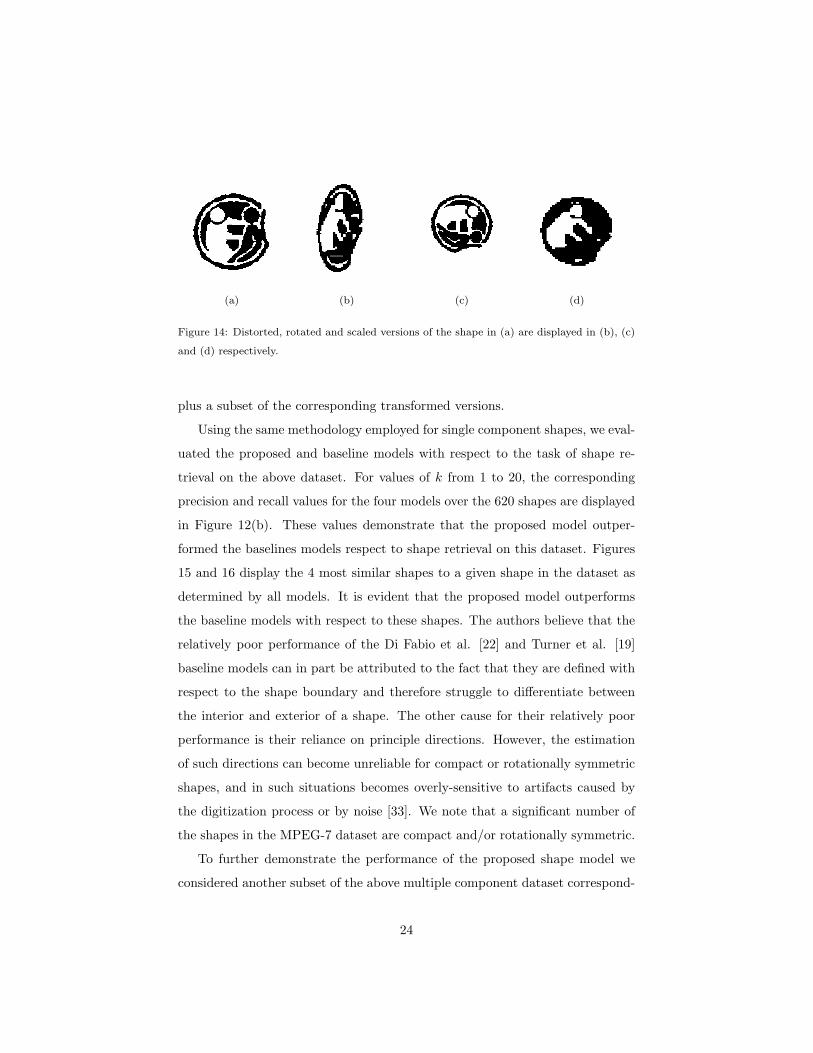
We evaluated the proposed shape model on a multiple component version of
the MPEG-7 shape dataset which contains in total 3,621 shapes [32]. A subset
of 620 shapes in this dataset consists of 31 individual shapes plus 9 distorted, 5
rotated and 5 scaled versions of each shape. A small distortion of a shape, such
as a small affine transformation, can result in topological changes which would
be considered to be very distinct unless a multi-scale perspective is considered.
For example two connected components which are spatially close may form
a single connected component following the application of a small distortion
transformation. Figure 14 displays one of the individual shapes in the dataset
22

(a) (b)
(c) (d)
(e) (f)
Figure 13: The persistence diagrams Persp(LS+
t ) and Persp(LS−
t ) corresponding to the shape
of Figure 2(a) are displayed in (a) and (b) respectively. The persistence diagrams Persp(LS+
t )
and Persp(LS−
t ) corresponding to the shape of Figure 2(b) are displayed in (c) and (d) re-
spectively. The persistence diagrams Persp(LS+
t ) and Persp(LS−
t ) corresponding to the shape
of Figure 2(c) are displayed in (e) and (f) respectively. In each figure elements of Pers0(.)
and Pers1(.) are represented using blue circles and green triangles respectively. Elements of
Pers0(.) that appear but do not disappear are determined to disappear at a value of ∞ and
are represented by a blue vertical arrow. Note that, two triangles exists at the location (0,35)
in the persistence diagrams of (d) and (f).
23
(a) (b) (c) (d)
Figure 14: Distorted, rotated and scaled versions of the shape in (a) are displayed in (b), (c)
and (d) respectively.
plus a subset of the corresponding transformed versions.
Using the same methodology employed for single component shapes, we eval-
uated the proposed and baseline models with respect to the task of shape re-
trieval on the above dataset. For values of k from 1 to 20, the corresponding
precision and recall values for the four models over the 620 shapes are displayed
in Figure 12(b). These values demonstrate that the proposed model outper-
formed the baselines models respect to shape retrieval on this dataset. Figures
15 and 16 display the 4 most similar shapes to a given shape in the dataset as
determined by all models. It is evident that the proposed model outperforms
the baseline models with respect to these shapes. The authors believe that the
relatively poor performance of the Di Fabio et al. [22] and Turner et al. [19]
baseline models can in part be attributed to the fact that they are defined with
respect to the shape boundary and therefore struggle to differentiate between
the interior and exterior of a shape. The other cause for their relatively poor
performance is their reliance on principle directions. However, the estimation
of such directions can become unreliable for compact or rotationally symmetric
shapes, and in such situations becomes overly-sensitive to artifacts caused by
the digitization process or by noise [33]. We note that a significant number of
the shapes in the MPEG-7 dataset are compact and/or rotationally symmetric.
To further demonstrate the performance of the proposed shape model we
considered another subset of the above multiple component dataset correspond-
24

(a)
(b) 5.7-3.2-85.2-74.8 (c) 6.7-3.0-154.6-251.7 (d) 7.0-3.1-86.4-73.2 (e) 7.4-3.7-84.0-71.5
(f) 7.6-2.8-29.1-38.1 (g) 7.8-2.8-74.1-68.5 (h) 8.5-2.9-79.2-66.9 (i) 6.7-3.0-154.6-251.7
(j) 7.6-2.8-29.1-38.1 (k) 27.5-17.1-71.3-79.0 (l) 7.8-2.8-74.1-68.5 (m) 27.8-17.6-75.1-90.4
(n) 7.6-2.8-29.1-38.1 (o) 8.5-2.9-79.2-66.9 (p) 7.6-3.2-77.2-66.9 (q) 35.8-20.8-95.0-68.5
Figure 15: For the query shape in (a), the four most similar shapes as determined by the
proposed, unsigned distance, Di Fabio et al. [22] and Turner et al. [19] models are displayed
in rows two, three, four and five respectively. In each row shapes are ordered from most
to least similar from left to right. The caption under each shape gives the respective dash
separated distances to the query shape.
25

(a)
(b) 6.9-4.1-760.2-
1441.1
(c) 17.4-11.0-923.2-
141.1
(d) 19.9-12.2-885.2-
129.2
(e) 20.8-14.4-1040.6-
706.8
(f) 6.9-4.1-760.2-
1441.1
(g) 17.4-11.0-923.2-
141.1
(h) 19.9-12.2-885.2-
129.2
(i) 57.1-12.3-947.9-
2311.6
(j) 83.3-30.2-657.5-
88.2
(k) 21.4-14.0-739.5-
4102.9
(l) 6.9-4.1-760.2-
1441.1
(m) 97.7-36.6-769.7-
1464.5
(n) 28.7-20.4-1013.8-
128.8
(o) 19.9-12.2-885.2-
129.2
(p) 22.5-15.7-111.3-
134.9
(q) 81.2-48.7-1325.2-
141.7
Figure 16: For the query shape in (a), the four most similar shapes as determined by the
proposed, unsigned distance, Di Fabio et al. [22] and Turner et al. [19] models are displayed
in rows two, three, four and five respectively. In each row shapes are ordered from most
to least similar from left to right. The caption under each shape gives the respective dash
separated distances to the query shape.
26

ing to the first 200 shapes in the dataset. Unlike the previous subset considered,
this subset is not formally structured and instead contains random shapes some
of which have a varying number of distorted versions. On this subset we per-
formed the task of retrieval using the same methodology described above. Figure
17 displays the three most similar shapes to four query shapes as determined
by the proposed model. It is evident that for the three query shapes in Fig-
ures 17(a), 17(e) and 17(i), the model retrieves shapes which are similar to the
query shape. However, for the query shape in Figure 17(m) the model does not
retrieve shapes which are similar to the query shape. This can be attributed to
the fact that although the query shape has distinctive features these features
are not topological in nature.
5. Conclusions
This paper proposes a novel shape model which is demonstrated to accu-
rately model multi-scale topological features. The proposed model is applicable
to both single and multiple component shapes and, to the authors knowledge,
is the first shape model to consider multi-scale topological features of multiple
component shapes.
The proposed model was evaluated both qualitatively and quantitatively
against three suitable baseline models using a number of datasets. This eval-
uation demonstrates that the proposed model fails to outperform one of the
baseline models with respect to the task of modelling single component shapes.
However, it outperforms both baseline models with respect to the task of mod-
elling multiple component shapes. The authors believe there exists scope to
develop a novel shape model which integrates the benefits of both the proposed
and baseline models.
Although in this paper we consider the specific problem of modelling two
dimensional shapes represented as binary images, the proposed model has the
potential to be applied to other problem instances. This includes modelling
three dimensional shapes represented as polygon meshes and modelling arbitrary
27

(a) (b) 17.90 (c) 20.14 (d) 22.86
(e) (f) 28.88 (g) 31.60 (h) 31.87
(i) (j) 0.00 (k) 38.95 (l) 46.36
(m) (n) 18.71 (o) 23.83 (p) 24.12
Figure 17: The first column of each row contains a query shape. The three most similar shapes
from most to least similar as determined by the proposed model are displayed in the second,
third and fourth columns respectively. The caption under each shape gives the corresponding
distance to the query shape as determined by the proposed model rounded to two decimal
places.
28

dimensional shapes represented as point clouds.
References
[1] D. Madsen, M. Luthi, A. Schneider, T. Vetter, Probabilistic joint face-
skull modelling for facial reconstruction, in: IEEE Conference on Computer
Vision and Pattern Recognition, 2018, pp. 5295–5303 (2018).
[2] J. C. Baker-LePain, K. R. Luker, J. A. Lynch, N. Parimi, M. C. Nevitt,
N. E. Lane, Active shape modeling of the hip in the prediction of incident
hip fracture, Journal of Bone and Mineral Research 26 (3) (2011) 468–474
(2011).
[3] N. Correll, K. E. Bekris, D. Berenson, O. Brock, A. Causo, K. Hauser,
K. Okada, A. Rodriguez, J. M. Romano, P. R. Wurman, Analysis and
observations from the first Amazon picking challenge, IEEE Transactions
on Automation Science and Engineering 15 (1) (2018) 172–188 (2018).
[4] F. P. Kuhl, C. R. Giardina, Elliptic fourier features of a closed contour,
Computer Graphics and Image Processing 18 (3) (1982) 236–258 (1982).
[5] T. Rauber, A. Steiger-Garcao, Shape description by UNL Fourier features
– an application to handwritten character recognition, in: International
Conference on Pattern Recognition, 1992, pp. 466–469 (1992).
[6] R. Mukundan, K. Ramakrishnan, Moment Functions in Image Analysis –
Theory and Applications, World Scientific, 1998 (1998).
[7] J. Flusser, B. Zitova, T. Suk, Moments and moment invariants in pattern
recognition, John Wiley & Sons, 2009 (2009).
[8] P. Corcoran, P. Mooney, A. Winstanley, A Convexity Measure for Open
and Closed Contours, in: British Machine Vision Conference, 2011 (2011).
[9] P. L. Rosin, Measuring shape: ellipticity, rectangularity, and triangularity,
Machine Vision and Applications 14 (3) (2003) 172–184 (2003).
29

[10] S. Belongie, J. Malik, J. Puzicha, Shape context: A new descriptor for
shape matching and object recognition, in: Advances in neural information
processing systems, 2001, pp. 831–837 (2001).
[11] F. Mokhtarian, A. K. Mackworth, A theory of multiscale, curvature-based
shape representation for planar curves, IEEE Transactions on Pattern Anal-
ysis & Machine Intelligence (8) (1992) 789–805 (1992).
[12] C. Asian, S. Tari, An axis-based representation for recognition, in: In-
ternational Conference on Computer Vision Volume 1, Vol. 2, 2005, pp.
1339–1346 (2005).
[13] K. B. Eom, Shape recognition using spectral features, Pattern Recognition
Letters 19 (2) (1998) 189 – 195 (1998).
[14] Z. You, A. K. Jain, Performance evaluation of shape matching via chord
length distribution, Computer vision, graphics, and image processing 28 (2)
(1984) 185–198 (1984).
[15] J. Zunic, P. L. Rosin, V. Ilic, Disconnectedness: A new moment invariant
for multi-component shapes, Pattern Recognition 78 (2018) 91–102 (2018).
[16] P. Corcoran, C. B. Jones, Modelling topological features of swarm be-
haviour in space and time with persistence landscapes, IEEE Access 5
(2017) 18534–18544 (2017).
[17] J. Curry, R. Ghrist, M. Robinson, Euler calculus with applications to sig-
nals and sensing, in: Symposia in Applied Mathematics, 2012 (2012).
[18] Z. Zhou, Y. Huang, L. Wang, T. Tan, Exploring generalized shape analysis
by topological representations, Pattern Recognition Letters 87 (2017) 177–
185 (2017).
[19] K. Turner, S. Mukherjee, D. M. Boyer, Persistent homology transform for
modeling shapes and surfaces, Information and Inference: A Journal of the
IMA 3 (4) (2014) 310–344 (2014).
30

[20] J. Curry, S. Mukherjee, K. Turner, How many directions determine a shape
and other sufficiency results for two topological transforms, arXiv preprint
arXiv:1805.09782 (2018).
[21] B. Di Fabio, C. Landi, Persistent homology and partial similarity of shapes,
Pattern Recognition Letters 33 (11) (2012) 1445–1450 (2012).
[22] B. Di Fabio, M. Ferri, Comparing persistence diagrams through complex
vectors, in: International Conference on Image Analysis and Processing,
Springer, 2015, pp. 294–305 (2015).
[23] M. Zeppelzauer, B. Zielinski, M. Juda, M. Seidl, A study on topological
descriptors for the analysis of 3d surface texture, Computer Vision and
Image Understanding 167 (2018) 74–88 (2018).
[24] A. Cerri, B. Di Fabio, F. Medri, Multi-scale approximation of the matching
distance for shape retrieval, in: Computational Topology in Image Context,
Springer, 2012, pp. 128–138 (2012).
[25] J. Munkres, Elements of Algebraic Topology, Westview Press, 1996 (1996).
[26] H. Edelsbrunner, J. Harer, Computational topology: an introduction,
American Mathematical Society, 2010 (2010).
[27] H. Edelsbrunner, J. Harer, Persistent homology – a survey, Contemporary
Mathematics 453 (2008) 257–282 (2008).
[28] A. Zomorodian, G. Carlsson, Computing persistent homology, Discrete &
Computational Geometry 33 (2) (2005) 249–274 (2005).
[29] M. Kerber, D. Morozov, A. Nigmetov, Geometry helps to compare per-
sistence diagrams, Journal of Experimental Algorithmics 22 (2017) 1–4
(2017).
[30] F. Chazal, B. Fasy, F. Lecci, B. Michel, A. Rinaldo, L. Wasserman, Robust
topological inference: Distance to a measure and kernel distance, Journal
of Machine Learning Research 18 (159) (2018) 1–40 (2018).
31

[31] R. Fabbri, L. D. F. Costa, J. C. Torelli, O. M. Bruno, 2D Euclidean distance
transform algorithms: a comparative survey, ACM Computing Surveys
40 (1) (2008) 2 (2008).
[32] M. Bober, MPEG-7 visual shape descriptors, IEEE Transactions on Cir-
cuits and Systems for Video Technology 11 (6) (2001) 716–719 (2001).
[33] J. Zunic, P. L. Rosin, L. Kopanja, On the orientability of shapes, IEEE
Transactions on Image Processing 15 (11) (2006) 3478–3487 (2006).
32