Georgia State UniversityScholarWorks @ Georgia State University

Real Estate Dissertations Department of Real Estate

8-7-2012

A Multi-Factor Probit Analysis of Non-PerformingCommercial Mortgage-Backed Security LoansPhilip SeagravesGeorgia State University

Follow this and additional works at: http://scholarworks.gsu.edu/real_estate_diss

This Dissertation is brought to you for free and open access by the Department of Real Estate at ScholarWorks @ Georgia State University. It has beenaccepted for inclusion in Real Estate Dissertations by an authorized administrator of ScholarWorks @ Georgia State University. For more information,please contact scholarworks@gsu.edu.

Recommended CitationSeagraves, Philip, "A Multi-Factor Probit Analysis of Non-Performing Commercial Mortgage-Backed Security Loans." Dissertation,Georgia State University, 2012.http://scholarworks.gsu.edu/real_estate_diss/13

i

Permission to Borrow

In presenting this dissertation as a partial fulfillment of the requirements for an advanced degree

from Georgia State University, I agree that the Library of the University shall make it available

for inspection and circulation in accordance with its regulations governing materials of this type.

I agree that permission to quote from or to publish this dissertation may be granted by the author

or, in his absence, the professor under whose direction it was written or, in his absence, by

the Dean of the Robinson College of Business. Such quoting, copying, or publishing must be

solely for scholarly purposes and must not involve potential financial gain. It is understood that

any copying from or publication of this dissertation that involves potential gain will not be

allowed without written permission of the author.

Philip Anthony Seagraves

ii

Notice to Borrowers

All dissertations deposited in the Georgia State University Library must be used only in

accordance with the stipulations prescribed by the author in the preceding statement.

The author of this dissertation is:

Philip Anthony Seagraves

35 Broad Street N.W.

Atlanta, GA 30303

The director of this dissertation is:

Dr. Jonathan A. Wiley

Department of Real Estate

Georgia State University

35 Broad Street N.W.

Atlanta, GA 30303

iii

A MULTI-FACTOR PROBIT ANALYSIS OF NON-PERFORMING COMMERCIAL

MORTGAGE-BACKED SECURITY LOANS

BY

PHILIP ANTHONY SEAGRAVES

Dissertation Submitted in Partial Fulfillment of the Requirements for the Degree

of

Doctor of Philosophy

in the Robinson College of Business

of

Georgia State University

GEORGIA STATE UNIVERSITY

ROBINSON COLLEGE OF BUSINESS

2012

iv

Copyright by

Philip Anthony Seagraves

2012

v

ACCEPTANCE

This dissertation was prepared under the direction of Philip Anthony Seagraves’ Dissertation

Committee. It has been approved and accepted by all members of that committee, and it has been

accepted in partial fulfillment of the requirements for the degree of Doctor of Philosophy in

Business Administration in the College of Business Administration of Georgia State University.

H. Fenwick Huss, Dean

College of Business Administration

DISSERTATION COMMITTEE:

Dr. Jonathan A. Wiley, Chair

Dr. Paul G. Gallimore

Dr. Karen M. Gibler

Dr. Alan J. Ziobrowski

Dr. Len V. Zumpano

vi

ABSTRACT

A MULTI-FACTOR PROBIT ANALYSIS OF NON-PERFORMING

COMMERCIAL MORTGAGE-BACKED SECURITY LOANS

By

Philip Anthony Seagraves

July 10, 2012

Committee Chair: Dr. Jonathan A. Wiley

Major Academic Unit: Real Estate

Commercial mortgage underwriters have traditionally relied upon a standard set of criteria for

approving and pricing loans. The increased level of commercial mortgage loan defaults from 1%

vii

at the start of 2009 to 9.32% by the end of 20111 provides motivation for questioning

underwriting standards which previously served the lending industry well. This dissertation

investigates factors that affect the probability of Non-performance among commercial mortgage-

backed security (CMBS) loans, proposes conditions under which the standard ratios may not

apply, and tests additional criteria which may prove useful during economic periods previously

not experienced by commercial mortgage underwriters. In this dissertation, Cap Rate Spread, the

difference between the cap rate of a property and the Coupon Rate of the associated loan, is

introduced to test whether the probability of Non-performance can be better predicted than by

relying on traditional commercial mortgage underwriting criteria such as Loan to Value (LTV)

and Debt Service Coverage Ratio (DSCR). Testing the research hypotheses with a probit model

using a database of 47,883 U.S. CMBS loans from 1993 to 2011, Cap Rate Spread is found to

have a significantly negative relationship with loan Non-performance. That is, as the Cap Rate

Spread falls, the probability of Non-performance rises appreciably.

A numerical model suggests that among loans which would have passed the standard ratio tests

requiring loans to have values of LTV less than .8 and DSCR greater than 1.25, a Cap Rate

Spread criteria requiring loans to have a value greater than 1% would have prevented the

origination of an additional 1,798 CMBS loans reducing the rate of Non-performance from

14.9% with only the LTV and DSCR criteria to just 11.6% by adding the Cap Rate Spread

1 Moody’s Investor Service: U.S. CMBS loan delinquencies rise to 9.32%, Global Credit Research, New York, January 20, 2012.

viii

criteria. Of course, adding additional criteria will also lead to errors of rejecting loans which

would have performed well. Back testing with the same sample of CMBS loans, this Type I error

rate rises from 19% with only the LTV and DSCR criteria to 34% with the addition of the Cap

Rate Spread.

Ultimately, CMBS loan underwriters must individually determine an acceptable level of Non-

performance appropriate to their business model and tolerance for risk. Using intuition,

experience, tools, and rules, each underwriter must choose a balance between the competing

risks of rejecting potentially profitable loans and accepting loans which will fail. This research

result is important because it helps deepen our understanding of the relationships between

property income and loan performance and provides an additional tool that underwriters may

employ in assessing CMBS loan risk.

ix

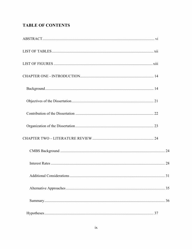
TABLE OF CONTENTS

ABSTRACT ....................................................................................................................... vi 

LIST OF TABLES ............................................................................................................ xii 

LIST OF FIGURES ......................................................................................................... xiii 

CHAPTER ONE - INTRODUCTION.............................................................................. 14 

Background ................................................................................................................... 14 

Objectives of the Dissertation ....................................................................................... 21 

Contribution of the Dissertation ................................................................................... 22 

Organization of the Dissertation ................................................................................... 23 

CHAPTER TWO – LITERATURE REVIEW ................................................................. 24 

CMBS Background ............................................................................................................... 24 

Interest Rates ......................................................................................................................... 28 

Additional Considerations ..................................................................................................... 31 

Alternative Approaches ......................................................................................................... 35 

Summary ................................................................................................................................ 36 

Hypotheses .................................................................................................................... 37 

x

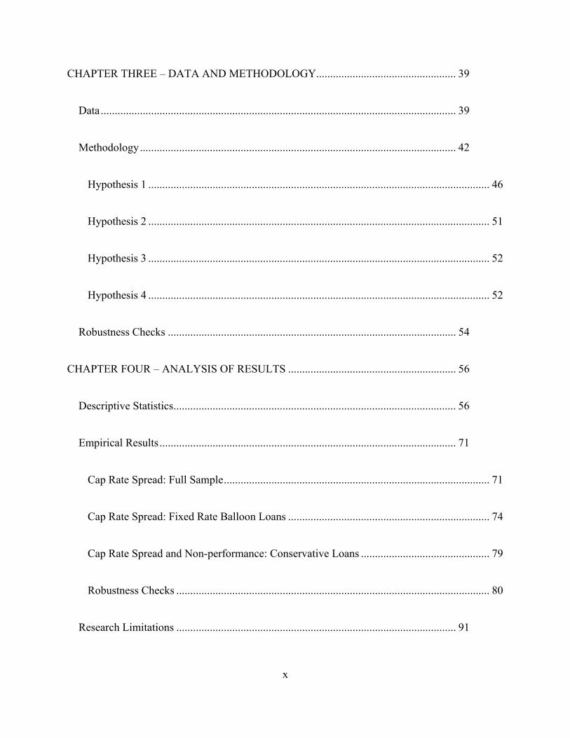
CHAPTER THREE – DATA AND METHODOLOGY .................................................. 39 

Data ............................................................................................................................... 39 

Methodology ................................................................................................................. 42 

Hypothesis 1 .......................................................................................................................... 46 

Hypothesis 2 .......................................................................................................................... 51 

Hypothesis 3 .......................................................................................................................... 52 

Hypothesis 4 .......................................................................................................................... 52 

Robustness Checks ....................................................................................................... 54 

CHAPTER FOUR – ANALYSIS OF RESULTS ............................................................ 56 

Descriptive Statistics ..................................................................................................... 56 

Empirical Results .......................................................................................................... 71 

Cap Rate Spread: Full Sample ............................................................................................... 71 

Cap Rate Spread: Fixed Rate Balloon Loans ........................................................................ 74 

Cap Rate Spread and Non-performance: Conservative Loans .............................................. 79 

Robustness Checks ................................................................................................................ 80 

Research Limitations .................................................................................................... 91 

xi

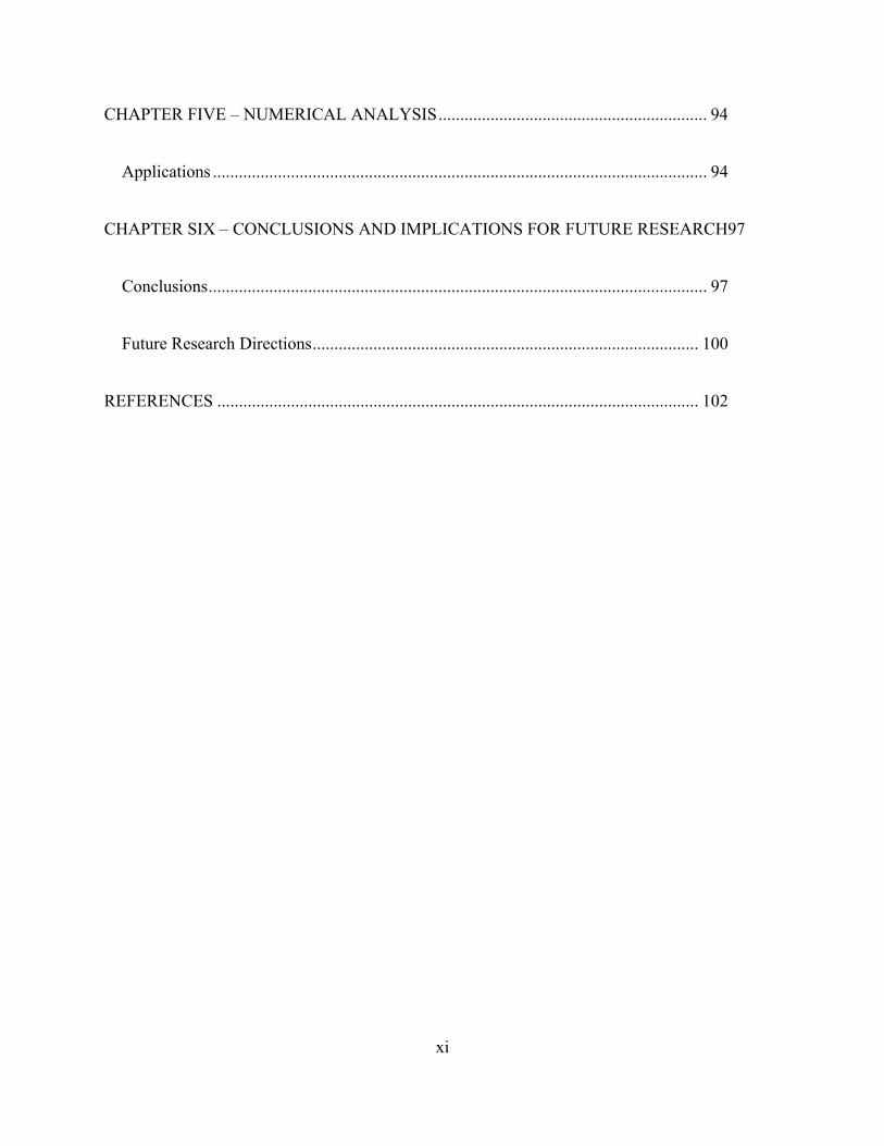
CHAPTER FIVE – NUMERICAL ANALYSIS .............................................................. 94 

Applications .................................................................................................................. 94 

CHAPTER SIX – CONCLUSIONS AND IMPLICATIONS FOR FUTURE RESEARCH97 

Conclusions ................................................................................................................... 97 

Future Research Directions ......................................................................................... 100 

REFERENCES ............................................................................................................... 102 

xii

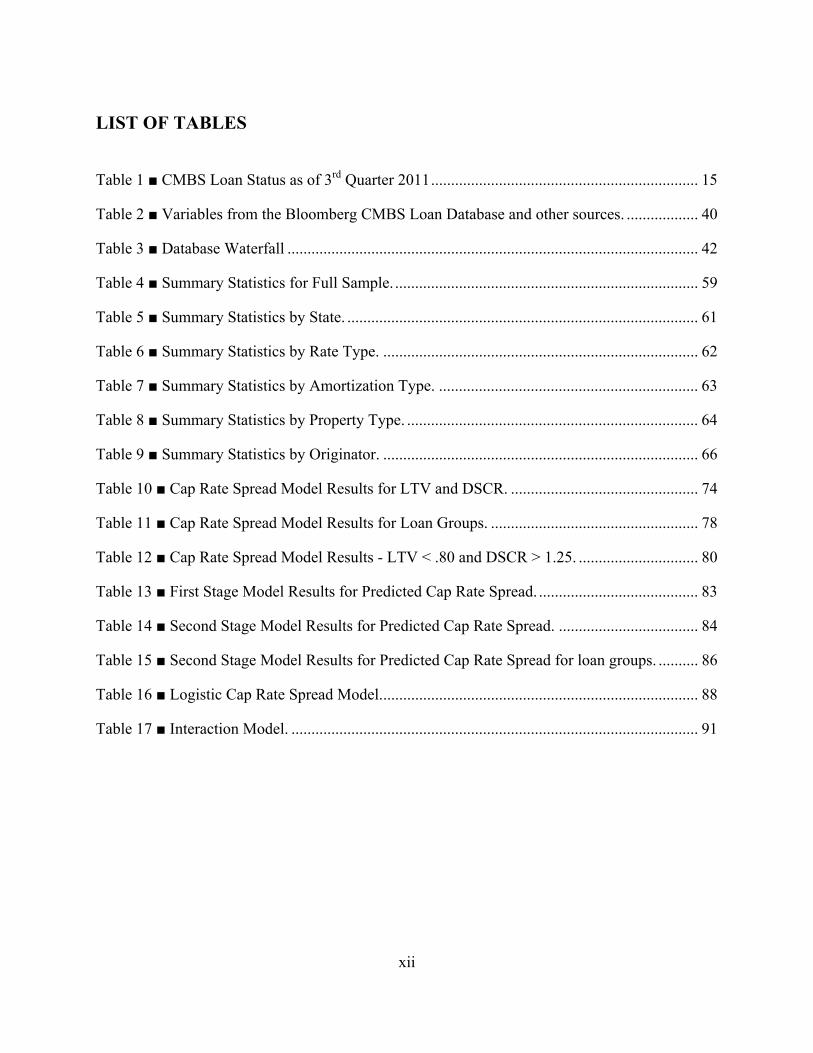
LIST OF TABLES

Table 1 ■ CMBS Loan Status as of 3rd Quarter 2011 ................................................................... 15 

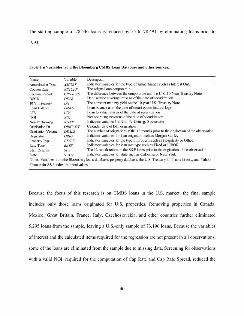
Table 2 ■ Variables from the Bloomberg CMBS Loan Database and other sources. .................. 40 

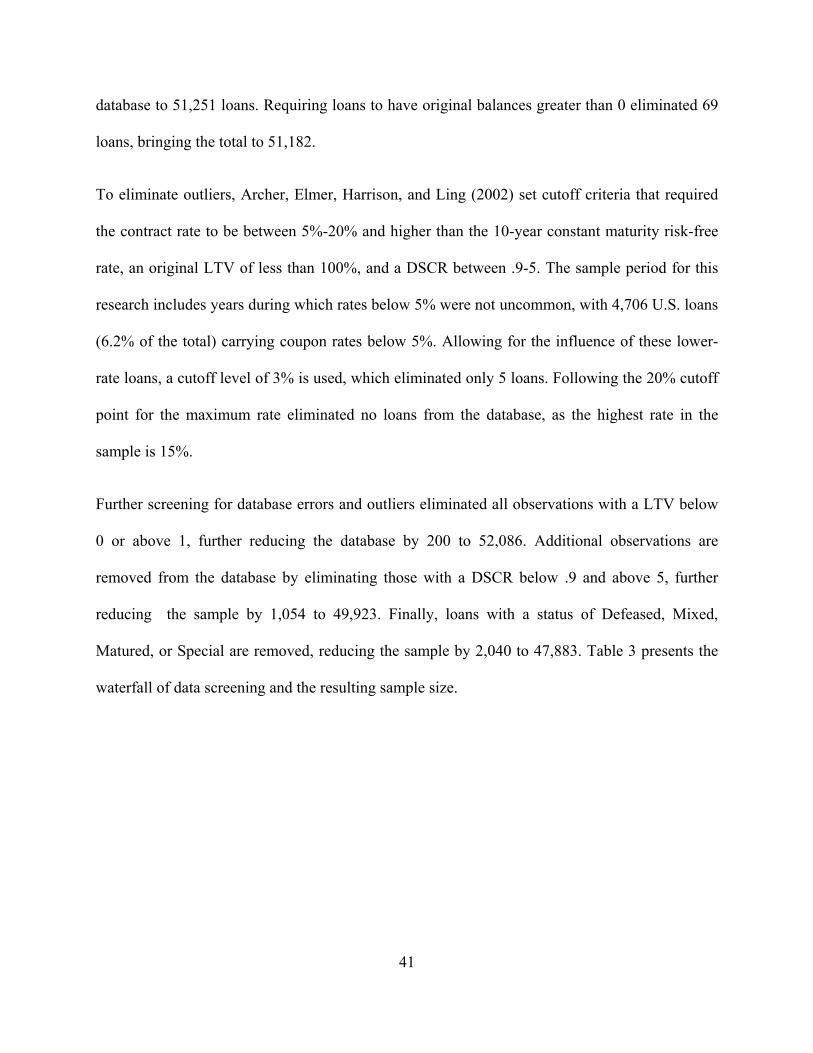
Table 3 ■ Database Waterfall ....................................................................................................... 42 

Table 4 ■ Summary Statistics for Full Sample. ............................................................................ 59 

Table 5 ■ Summary Statistics by State. ........................................................................................ 61 

Table 6 ■ Summary Statistics by Rate Type. ............................................................................... 62 

Table 7 ■ Summary Statistics by Amortization Type. ................................................................. 63 

Table 8 ■ Summary Statistics by Property Type. ......................................................................... 64 

Table 9 ■ Summary Statistics by Originator. ............................................................................... 66 

Table 10 ■ Cap Rate Spread Model Results for LTV and DSCR. ............................................... 74 

Table 11 ■ Cap Rate Spread Model Results for Loan Groups. .................................................... 78 

Table 12 ■ Cap Rate Spread Model Results - LTV < .80 and DSCR > 1.25. .............................. 80 

Table 13 ■ First Stage Model Results for Predicted Cap Rate Spread. ........................................ 83 

Table 14 ■ Second Stage Model Results for Predicted Cap Rate Spread. ................................... 84 

Table 15 ■ Second Stage Model Results for Predicted Cap Rate Spread for loan groups. .......... 86 

Table 16 ■ Logistic Cap Rate Spread Model. ............................................................................... 88 

Table 17 ■ Interaction Model. ...................................................................................................... 91 

xiii

LIST OF FIGURES

Figure 1 ■ CMBS Loan Originations per Year ............................................................................ 16 

Figure 2 ■ Cap Rate Spread and Market Yield on 10-Year Treasuries ........................................ 19 

Figure 3 ■ Loan Performance with LTV/DSCR and Cap Rate Spread Rules .............................. 95 

14

CHAPTER ONE - INTRODUCTION

Background

Standard underwriting models for commercial loans rely upon classic measures such as the size

of the loan relative to the value of the property (Loan to Value Ratio, LTV) and the ratio of net

income from the property to the size of the annual debt payments (Debt Service Coverage Ratio,

DSCR) for approving and pricing debt. LTV and DSCR are presented in equations (1) and (2)

respectively.

Loan to Value LTV = Original Loan Balance (LOAN)

Project Value (VALUE) (1)

DebtServiceCoverageRatio DSCR (2)

LTV is a widely used measure of loan risk and one of the most commonly cited features, along

with interest rates, used to describe individual deals and the general debt environment. As the

loan amount approaches or surpasses the value of the underlying asset, the default risk increases.

This risk is also a function of other factors such as the experience of the borrower, the type of

project, geography, the state of the economy, and competition.

DSCR is also an important criterion used by loan underwriters to determine the riskiness of a

loan. This measure provides a simple indicator of a borrower’s ability to continue making their

debt payments in the face of reduced rental income or increased expenses. As the DSCR rises,

the borrower has a greater cushion against rent pressures, tenant turnover, unexpected expenses,

or the effects of natural disasters for maintaining their debt service obligations. As with LTV, the

15

ability of DSCR to provide a valuable risk screening function may be related to other economic

factors such as market interest rates.

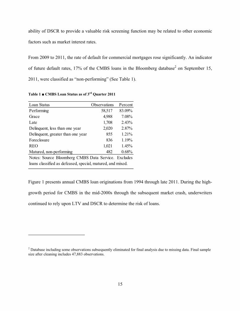
From 2009 to 2011, the rate of default for commercial mortgages rose significantly. An indicator

of future default rates, 17% of the CMBS loans in the Bloomberg database2 on September 15,

2011, were classified as “non-performing” (See Table 1).

Table 1 ■ CMBS Loan Status as of 3rd Quarter 2011

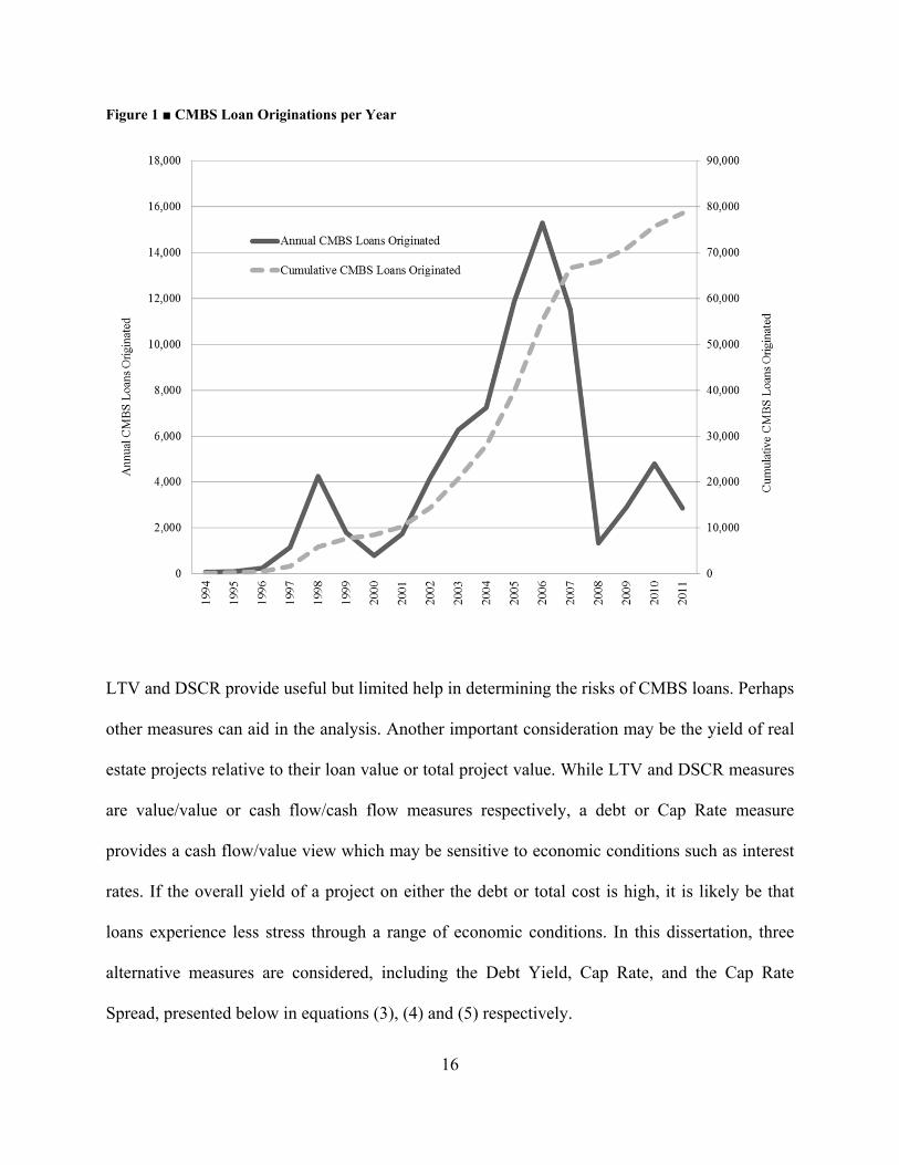
Figure 1 presents annual CMBS loan originations from 1994 through late 2011. During the high-

growth period for CMBS in the mid-2000s through the subsequent market crash, underwriters

continued to rely upon LTV and DSCR to determine the risk of loans.

2 Database including some observations subsequently eliminated for final analysis due to missing data. Final sample size after cleaning includes 47,883 observations.

Loan Status Observations PercentPerforming 58,517 83.09%Grace 4,988 7.08%Late 1,708 2.43%Delinquent, less than one year 2,020 2.87%Delinquent, greater than one year 855 1.21%Foreclosure 836 1.19%REO 1,021 1.45%Matured, non-performing 482 0.68%Notes: Source Bloomberg CMBS Data Service. Excludesloans classified as defeased, special, matured, and mixed.

16

Figure 1 ■ CMBS Loan Originations per Year

LTV and DSCR provide useful but limited help in determining the risks of CMBS loans. Perhaps

other measures can aid in the analysis. Another important consideration may be the yield of real

estate projects relative to their loan value or total project value. While LTV and DSCR measures

are value/value or cash flow/cash flow measures respectively, a debt or Cap Rate measure

provides a cash flow/value view which may be sensitive to economic conditions such as interest

rates. If the overall yield of a project on either the debt or total cost is high, it is likely be that

loans experience less stress through a range of economic conditions. In this dissertation, three

alternative measures are considered, including the Debt Yield, Cap Rate, and the Cap Rate

Spread, presented below in equations (3), (4) and (5) respectively.

17

Debt Yield (DYLD)=Net Operating Income (NOI)

Original Loan Balance (LOAN) (3)

Cap Rate (CAPRT) =Net Operating Income (NOI)

Project Value (VALUE) (4)

Cap Rate Spread (SPREAD) = CAPRT – Coupon, (5)

where Coupon is the net coupon rate on the loan. If LTV and DSCR were limited in their ability

to predict loan default leading up to the recent market crash, perhaps their usefulness declined as

interest rates fell. If so, other measures such as Debt Yield, Cap Rate, and the Cap Rate Spread

may have emerged as important criteria in assessing risk and should be used to complement

other methods and improve overall default prediction reliability. It can be shown that Debt Yield,

as defined above, is simply the Cap Rate divided by the LTV at origination for the loan. A

simple example makes the connection quite clear: a project valued at 100 with a loan of 70 will

have a LTV of .7 and, if the NOI is 10, the Cap Rate will be .1 and the Debt Yield .14 calculated

as either 10/70 or .1/.7. Acknowledging that both Debt Yield and Cap Rate may provide further

insights into the factors related to CMBS loan performance, I focus on the measure Cap Rate

Spread for the remainder of this dissertation.

During the critical phase of CMBS history beginning in the mid-1990s through today, interest

rates have experienced periods of both falling and rising and have dropped to less than half of

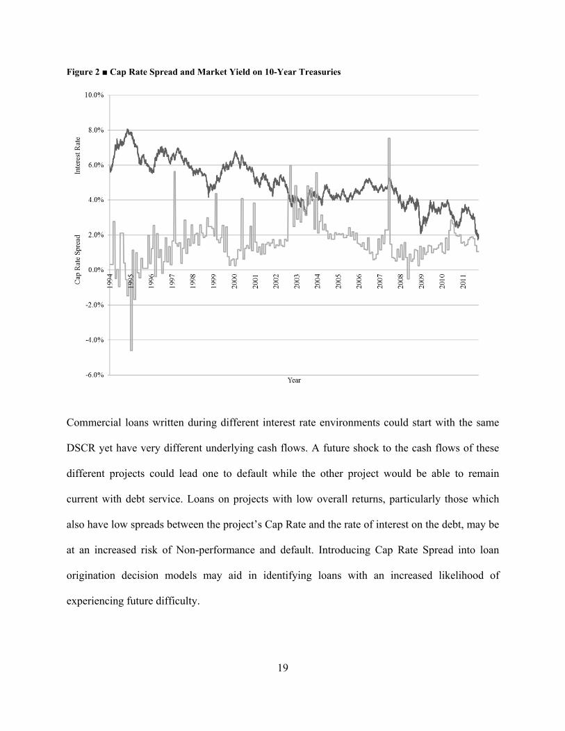
what they were at the beginning of this time period. Figure 2 shows that in the mid-1990s, rates

on 10-Year Treasuries were around 7% and eventually fell below 2% in the fourth quarter of

2011. The second series on Figure 2 (the lighter line) shows the Cap Rate Spread over the course

of the sample period. This series is expected to move in the opposite direction of interest trends

as the Cap Rate Spread is constructed using the coupon rate on the loan.

18

Prior to 2003, the negative relationship appears clear in both direction and magnitude of the rate

swings. However, the period after 2003 appears to have changed somewhat with a period of

relatively stable interest rates coupled with Cap Rate Spreads which fell from 4% in 2003 to 1%

in 2007. Even more noticeable beginning in 2007, the relationship seems to have become

positive with successive periods during which both rates appear to fall or rise together. This

seeming change provides a backdrop and further motivation for this study and may explain an

increased role for Cap Rate Spread in predicting loan Non-performance in the more recent

periods. The relationship between market interest rates and Cap Rate Spread may have changed

during this period and merits further investigation confirming the change and testing hypothetical

causes, if any.

19

Figure 2 ■ Cap Rate Spread and Market Yield on 10-Year Treasuries

Commercial loans written during different interest rate environments could start with the same

DSCR yet have very different underlying cash flows. A future shock to the cash flows of these

different projects could lead one to default while the other project would be able to remain

current with debt service. Loans on projects with low overall returns, particularly those which

also have low spreads between the project’s Cap Rate and the rate of interest on the debt, may be

at an increased risk of Non-performance and default. Introducing Cap Rate Spread into loan

origination decision models may aid in identifying loans with an increased likelihood of

experiencing future difficulty.

20

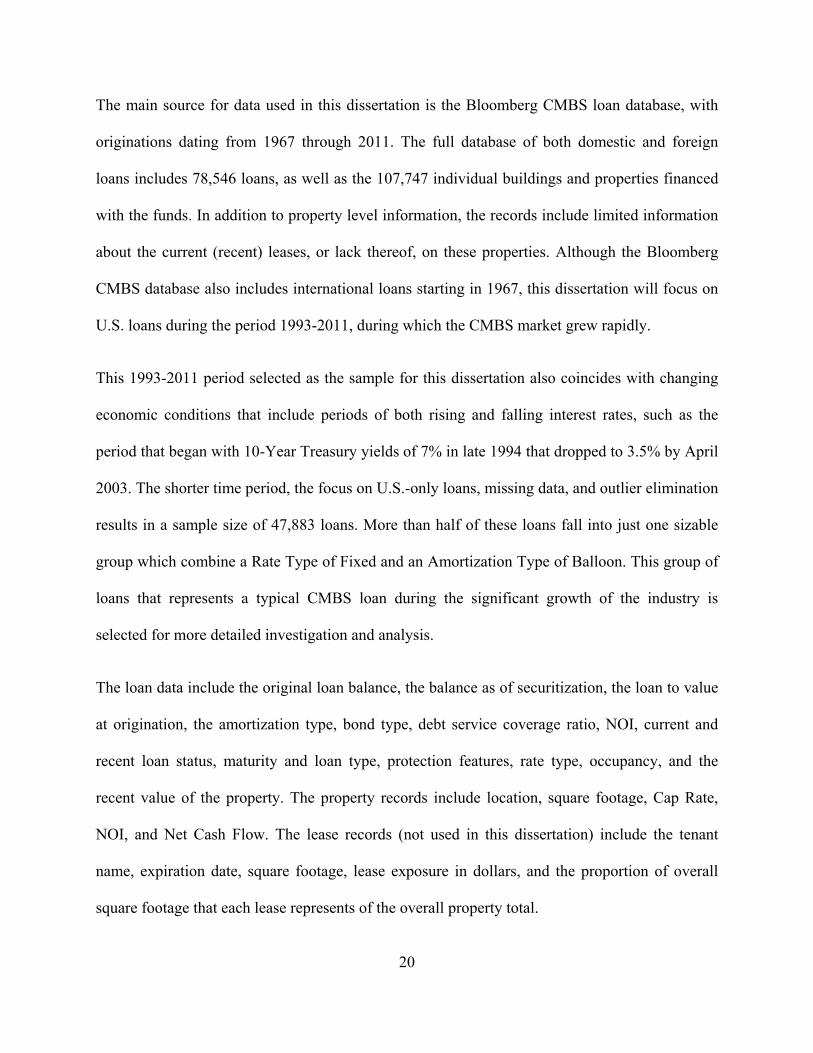
The main source for data used in this dissertation is the Bloomberg CMBS loan database, with

originations dating from 1967 through 2011. The full database of both domestic and foreign

loans includes 78,546 loans, as well as the 107,747 individual buildings and properties financed

with the funds. In addition to property level information, the records include limited information

about the current (recent) leases, or lack thereof, on these properties. Although the Bloomberg

CMBS database also includes international loans starting in 1967, this dissertation will focus on

U.S. loans during the period 1993-2011, during which the CMBS market grew rapidly.

This 1993-2011 period selected as the sample for this dissertation also coincides with changing

economic conditions that include periods of both rising and falling interest rates, such as the

period that began with 10-Year Treasury yields of 7% in late 1994 that dropped to 3.5% by April

2003. The shorter time period, the focus on U.S.-only loans, missing data, and outlier elimination

results in a sample size of 47,883 loans. More than half of these loans fall into just one sizable

group which combine a Rate Type of Fixed and an Amortization Type of Balloon. This group of

loans that represents a typical CMBS loan during the significant growth of the industry is

selected for more detailed investigation and analysis.

The loan data include the original loan balance, the balance as of securitization, the loan to value

at origination, the amortization type, bond type, debt service coverage ratio, NOI, current and

recent loan status, maturity and loan type, protection features, rate type, occupancy, and the

recent value of the property. The property records include location, square footage, Cap Rate,

NOI, and Net Cash Flow. The lease records (not used in this dissertation) include the tenant

name, expiration date, square footage, lease exposure in dollars, and the proportion of overall

square footage that each lease represents of the overall property total.

21

Objectives of the Dissertation

The overall objective for this dissertation is to extend the body of knowledge regarding an

important aspect of the real estate debt market—the performance of loans underwritten for the

CMBS market. The specific questions of interest addressed in this dissertation are as follows:

1. Can measures other than LTV and DSCR, such as Cap Rate Spread, provide additional

information useful in predicting default of CMBS loans?

2. How do the typical Fixed Rate Balloon loans differ from other loans in their relationships

between Non-performance and underwriting ratios such as LTV, DSCR and Cap Rate

Spread?

3. During the recent financial crisis, could reliance on Cap Rate Spread have provided

additional protection against future loan Non-performance?

To answer these questions, the relationships between the probability of Non-performance and the

variables of interest, LTV, DSCR, and Cap Rate Spread are estimated with probit models. In

addition to these variables of interest, the models also include variables which control for interest

rates, recent stock market performance, loan interest rate, recent origination activity, loan size,

and indicators for categorical variables such as rate type, amortization type, originating firm and

property type. To test for sensitivity to the endogeneity between loan coupon rates and the ratios

LTV and DSCR, I estimate the Non-performance relationships with a two-stage model which

first estimates a predicted coupon rate. This predicted coupon rate is used to construct the Cap

Rate Spread variable in the second stage of the model.

22

Sensitivity to the distribution assumption is tested by substituting a logistic model, with a logistic

distribution, for the probit approach, which relies upon a cumulative normal distribution. Using

typical screening criteria for LTV and DSCR, the analysis is performed with a sample of loans

which would meet conservative underwriting standards to determine how Cap Rate Spread

would perform among these presumably safe loans. Finally, a numerical analysis is undertaken

to estimate the quantity of CMBS loans which would have been avoided following the

conservative LTV/DSCR criteria and the additional loans which would have been avoided by

adding a Cap Rate Spread floor. As a part of this numerical analysis, a limited type I error rate-

like approach suggests the quantity of currently performing loans which would have never been

originated had a Cap Rate Spread floor been utilized. One must be cautious in this regard as it

may be that many of these loans predicted by Cap Rate Spread to be in a non-performing state

have simply not entered this state… yet. Understanding the full extent of the Type II error, loans

that are still performing but ultimately doomed to fail, is necessarily a matter of time.

Contribution of the Dissertation

This dissertation extends the real estate finance literature by proposing and testing new

hypotheses about factors important in estimating the risks of commercial mortgages. Industry

practice and the academic literature regard the traditional measures of LTV and DSCR as the

primary criteria in underwriting commercial mortgages. This dissertation builds upon this

foundation by taking into account additional considerations which may aid in predicting the

performance of CMBS loans.

23

This dissertation takes a fresh approach to modeling the probability of CMBS loan default. The

methodology incorporates variables described by past research, such as LTV, DSCR, and

property type, but extends the scope of past work by adding factors such as Cap Rate Spread and

exploring both the theoretical and practical implications of relying upon a Cap Rate Spread

underwriting rule for CMBS loans. Using both single- and two-stage probit regression and

numerical analysis, the expanded set of explanatory variables is incorporated into a model to

estimate the probability of CMBS loan default and provides a hypothetical view of the

consequences of relying on an additional underwriting rule based on the results.

To provide a background and theoretical foundation for the effects of regulatory and market

events, this dissertation also documents and presents a historical perspective on the outside

forces influencing origination decisions and how these decisions may have played a role in

subsequent loan defaults in the CMBS pools. By extending the literature on CMBS loan default

with factors such as recent loan origination activity, Cap Rate Spread, and introducing the

potential effects on originator behavior induced by a changing regulatory environment, this

dissertation adds to the collective knowledge of real estate finance and related disciplines.

Organization of the Dissertation

The balance of this dissertation is organized as follows: Chapter Two presents a background of

past and current literature and the hypotheses tested in this dissertation; Chapter Three describes

the data and methodologies employed in this dissertation; Chapters Four, Five, and Six present

the results, a numerical analysis, and conclusions, respectively. The dissertation concludes with a

list of references.

24

CHAPTER TWO – LITERATURE REVIEW

This chapter begins with a brief background of the CMBS market and a review of the academic

research findings relating LTV and DSCR to CMBS loan performance and default. The literature

on LTV and DSCR helps establish a foundation for this research by providing guidance on

empirical methods, control variables and robustness measures. The next section discusses

research findings which suggest additional factors related to default, alternative methodologies,

related theories, and a broader look at loan default where the intersection between performance

and default theory and methodology overlap with the CMBS market.

CMBS Background

Although the earliest CMBS loans recorded in the Bloomberg database date to the 1960s, the

early-1990s saw an increasing acceptance of residential and commercial mortgage-backed

securities with the mid- to late 1990s marked by the introduction of CMBS holding loans

specifically originated for ultimate securitization. The Financial Institutes Reform, Recovery and

Enforcement Act (FIRREA), and the resulting Resolution Trust Corporation (RTC) provided the

impetus for CMBS growth through their efforts to liquidate the enormous real estate portfolios of

the failed thrifts. The sample period under study also includes a myriad of legislative initiatives

and changes such as SEC Regulation AB, Basel, the Volcker Rule, FDIC Safe Harbor, and

Dodd-Frank, which may impact the incentives and resulting behavior of CMBS loan

underwriters now and into the future.

The emergence of another securitization option in the mid2000s, collateralized debt obligations

(CDOs), may also have influenced the origination standards of CMBS originators. In an

25

environment with fewer restrictions on borrowers, the CDO alternative may have provided a

more attractive option for those wishing to access a capital market hungry for yield and willing

to invest heavily in commercial real estate. This competition for loans may have lead CMBS

underwriters to relax their standards by offering higher LTVs and lower DSCRs to stave off an

erosion of market share in a blossoming CDO market that typically provided floating rate terms

and less onerous prepayment limitations.

Commercial mortgage default, which had a significant impact on insurance companies and

pension funds throughout the 1980s, received a great deal of attention in the academic

community. Since then, subjects such as the factors contributing to default, models of default

probability, the valuation of prepayment and default options, and pricing have regularly appeared

in prominent real estate, finance, and economics journals (Kau, Keenan, Muller III, and

Epperson 1987; Vandell 1984; Vandell 1992). Research as early as the pioneering study by

Vandell (1984) points out that using the models designed for residential default are inadequate

because of the income-producing nature of commercial real estate and the differing economic

sensitivities inherent in these distinct debt instruments. Vandell (1984) also suggests that the

simple ratio tests in use at the time, such as LTV and DSCR, would not provide the intended

information to help keep default risk below some predetermined level. The author contends that

default prediction models should include information about the property such as location.

Vandell (1984) further posits that economic conditions such as interest rates, which change over

time, are also important factors that affect the performance of commercial mortgages. In a

detailed evaluation of the traditional ratio measures, the author also suggests that these ratios are

woefully inadequate because they fail to make the connection between cash flows and the equity

26

in a framework where cash flows and equity are volatile over time and may exhibit varying

volatility between borrowers. This observation provides an important motivation for the

investigation in this dissertation of Cap Rate Spread which makes the connection between cash

flows and equity.

In one of the first works on the growing field of CMBS, Kau, Keenan, Muller, and Epperson

(1987) identify two default scenarios: the first is when the value of the collateral is less than the

outstanding balance of the loan; the second, when the collateral is worth more than the balance

of the loan. The authors point out that for the second type of default to occur, there must be a

large spread between market and contract interest rates during the prepayment lockout period. If

not for the lockout period, prepayment rather than default would be the result when the property

value is greater than the loan balance. This insight suggests that newer loans, which are more

likely to be within the lockout period, are more prone to default with falling interest rates than

loans which are older and more likely to be past the lockout date. Loans originated later in the

sample period, thus more likely to be in the lockout period, and also faced with falling interest

rates may be particularly susceptible to entering a state of Non-performance or default. This

condition, along with the use of interest rate control variables, further motivates the study of

Non-performance and the relationship between interest rate spread measures such as Cap Rate

Spread.

The Kau, Keenan, Muller, and Epperson (1987) model assumed borrowers would exhibit what

they termed “ruthless default,” which means that borrowers would default as soon as their equity

value fell below the mortgage value. Their model also assumed no transaction costs for default.

Vandell (1992) challenged these assumption by testing an alternative theoretical model of

27

rational default in the presence of transaction costs and found that surprisingly few borrowers

defaulted even when LTV exceeded 1.1, a state in which borrowers are significantly “under

water”. Allowing for the possibility that some loans with high LTV were restructured, 75-85% of

loans in this high-LTV category were retained by both borrower and lender, presumably to avoid

the high costs of default.

Although the Vandell (1992) study—which uses quarterly data to relate the incidence of default

to contemporaneous measures of LTV—focuses on contemporaneous measures influencing the

probability of default, several features of the research provide guidance for this dissertation.

Focusing on regions such as the South and the manner in which current interest rates affect the

market value of the loans, the study points out the importance of both geography and interest-rate

trends in predicting commercial mortgage default. In an interesting extension, Vandell (1992)

uses simulation to project, under varying scenarios, the future of mortgage defaults, suggesting

that foreclosure rates would double by 1993.

Following the widespread collapse of savings and loans and the subsequent large-scale

commercial real estate liquidation by the Resolution Trust Corporation, the subject of loan

default moved to the forefront in the eyes of academic researchers in a wide range of business

disciplines including finance, economics, and real estate. In an evaluation of apartment

mortgages and the factors leading to default, Archer, Elmer, Harrison, and Ling (2002) found

that LTV was not related to default. Their conclusion suggests that LTV is a primary factor in

pricing loans with lower-risk borrowers who are offered higher LTV debt structures. As a result,

loan pricing (interest rate) and LTV are jointly determined. This endogeneity hypothesis is

supported by their results, which also found property characteristics such as location and cash

28

flow at the time of origination (DSCR) to be the primary factors in predicting default in their

sample of multifamily mortgages from 1991-1996. The sample of the Archer, Elmer, Harrison,

and Ling (2002) study, comprising 495 loans securitized by the RTC and FDIC, covered only a

brief period of CMBS history and a much smaller number of loans than this dissertation utilizes.

With the benefit of an increased sample size and longer period of time covering a variety of

economic conditions, this dissertation should better detect and interpret the factors related to loan

defaults while carefully considering potential endogeneity issues.

Interest Rates

As the market for CMBS was blossoming, Gallo, Buttimer, Lockwood, and Rutherford (1997)

studied the performance of mutual funds holding mortgage-backed securities (MBS) relative to a

variety of market benchmarks. Using single- and multi-index models, they found that MBS

mutual funds underperformed other mutual funds and provided evidence that this was

attributable to fund expenses, MBS selection, and timing. Gallo, Buttimer, Lockwood, and

Rutherford (1997) also found that the effects were sensitive to periods of rising and falling

interest rates.

When interest rates were rising, the MBS mutual funds underperformed, while no such result

was detected during periods of falling interest rates. The authors also found that performance

was heavily influenced by outlier periods, with performance more than two standard deviations

away from the mean monthly returns. This result suggests that influences on the performance of

MBS may change over time and that a long time series may mask dynamic relationships.

29

Commercial mortgage default and prepayment may also be evaluated in a competing risks

framework wherein the borrower may, in any period, take one of three actions: prepay, default,

or remain current. Ambrose and Sanders (2003) model the prepayment option as a function of

changing interest rates relative to the loan coupon rate while taking into account the effects of

prepayment lockouts and yield maintenance provisions that may be a part of individual loan

agreements. Recognizing that interest rate expectations may affect the prepayment outcome, the

authors also incorporate a yield curve variable into their empirical method: the spread between 1-

Year and 10-Year Treasury rates. Since their analysis views prepayment and default as options, a

measure of volatility is required to appropriately value the option. For interest rates, Ambrose

and Sanders (2003) include a rolling standard deviation of the prior 24 months of the 10-Year

Treasury.

Ambrose and Sanders (2003) find a significant and positive relationship between interest rate

spreads and the loan coupon rates. Significant relationships were also found between default and

both the term spread and interest-rate volatility, with the former being negative and the latter

positive. In contrast to other results described in this dissertation, the authors found no significant

relationship between LTV at the time of origination and default, though they did find that these

higher LTV mortgages were more likely to prepay.

Also using a proportional hazard with competing risks, Ciochetti, Deng, Lee, Shilling, and Yao

(2003) test for factors contributing to default and prepayment. In addition to the typical ratios at

the time of origination, the authors use an estimate of contemporaneous DSCR and LTV on a

quarterly basis using changes in the NCREIF property appreciation and the NCREIF income

yield to approximate what would have happened at a property level if the values and incomes

30

were affected in the same way as the other properties represented by the NCREIF data.

Reasoning that the effects may vary depending upon the size of the loan, the authors also

incorporate dummy variables for small, medium, and large.

Ciochetti and his colleagues found that the contemporaneous DSCR was significant and

negatively related to the probability of default, while the DSCR at origination was insignificant.

Similarly, the authors found that as contemporaneous LTV rose, so did the probability of default,

though in a non-linear fashion. They also found significant increases in default probability

among medium and large loans, balloon loans, and loans with a smaller spread between the

coupon rate and 10-Year Treasury rates. The study used dummy variables for the different

property types but found none to be significantly related to default probability or prepayment. To

eliminate potential originator bias, this study used a weighting technique to make the smaller

sample better fit the population.

The Ciochetti et al. (2003) study uses a sample of 2,043 commercial loans from one large

insurance company with quarterly detail on default and prepayment. Their proportional hazard

model with competing risks takes advantage of the quarterly data and provides a clear picture of

how default and prepayment unfold over time but the larger sample of nearly 50,000 loans

collected and analyzed for this dissertation spans a longer time period and provides additional

insights into the relationships between loan features at origination and subsequent Non-

performance.

In one of the early studies of the CMBS market, Childs, Ott, and Riddiough (1996) refer to

CMBS as “a new and increasingly important class of structured debt.” Their work considers

CMBS loan default risk in the context of CMBS tranche pricing. They employ a two-stage

31

approach that first estimates the points at which borrowers in the pool will default and then uses

Monte Carlo analysis to “follow” the loans through various paths while iterating interest rate and

property price state variables. The findings for the senior tranche indicate that higher rates of

default correlate with low rate outcomes. Finding positive correlation between interest rates and

property values, the authors further suggest that the low rates would be associated with larger

loans and higher probabilities of default. Their findings provide further motivation for evaluating

the relationships between Non-performance and the level of interest rates, the size of loans, and

the spread between Cap Rates and the interest rates on the loans, Cap Rate Spread.

Additional Considerations

Other factors and events such as geography, originators, property types, legislative changes,

industry dynamics, and competition from new investment vehicles may affect performance of

properties or the decision-making process at origination and lead to differences in the probability

of Non-performance or default among commercial mortgages.

While the information available at the time of origination provides valuable insight into the

probability of default of a commercial mortgage, it may also be the case that events that occur

after origination affect the ultimate performance of a loan. A downturn in local economic

conditions surrounding the properties funded by each loan may also put pressure on a borrower’s

ability to repay the debt. Conversely, a strong local economy may provide some measure of

protection against default even for highly leveraged commercial real estate projects. Using a

regional analysis, Archer, Elmer, Harrison, and Ling (2002) incorporate home price appreciation,

wage rates, per capita incomes, and employment levels, and found significant differences among

32

several of the regions identified by the National Council of Real Estate Investment Fiduciaries

(NCREIF).

Using only loan level data may ignore important information in estimating the probability of

default. Characteristics of the property such as type, size, and number of tenants may also

provide insight at origination as to the default probability of CMBS loans. Archer, Elmer,

Harrison, and Ling (2002) incorporate multifamily property level information such as number of

units, price per unit, year the building was completed, and whether the property is located in a

judicial foreclosure state. They found that only the property age was significant in their logistic

model.

When holding out the entire group of property level characteristics, tests for significance (change

in Pseudo R2, and Chi-Square) indicate that, as a group, the property level characteristics are

more important than any other group of variables, including LTV, DSCR, financial institution,

post-origination MSA factors, and location of the collateral. Though the property level factors

dominate, property location significantly affects default probability. These results indicate that

loan underwriters do not fully adjust their origination criteria to account for these property level

and location risks. A sample with far more observations in each geographic cell may provide

further insights into this dimension of loan default outcomes.

Following the Gallo, Buttimer, Lockwood, and Rutherford (1997) study of MBS mutual fund

returns, Xu and Fung (2005) investigated the returns of an important residential MBS index.

Estimating the relationships using a VAR model with data from 1988 through 2001, the authors

found, among other factors, that index returns are related to interest rates, term structures, and

new home sales. Their results were confirmed by using variance decomposition and impulse

33

response techniques. The authors break their sample period into two periods to discern the

effects of the introduction of the Office of Housing Enterprise Oversight (OFHEO) in 1992.

They posit that the introduction of this governmental entity may have altered the risks inherent in

the MBS market. By analyzing the sample during these two regimes, the authors found evidence

of a structural change in the MBS market after which investors recognized that these securities

may be exposed to greater risk than previously assumed. This study suggests that the

introduction of regulatory and statutory events into a set of variables provides important insight

into how the CMBS market has developed over the last twenty years.

Titman and Tsyplakov (2010) studied the characteristics of commercial mortgage originators and

found that loans originated by recent stock price losers tended to default more often than loans of

other firms. They also found that broad financial market performance was an important factor,

with differences greater during significant market downturns. This result provides motivation for

including broad market indicators, such as interest rates, in the new models, as these may also

affect the probability of default for firms originating during these periods and may also affect

individual originators differently.

The authors ascribe the effects to firms choosing short-term profits at the expense of their

reputation. Firms earned short-term profits in the form of origination fees by lowering their

underwriting standards and taking on riskier loans. This hypothesis is supported by evidence that

ratings agencies tend to assign lower scores to pools that contain loans from underwriting firms

whose stock price have seen recent declines, firms more likely to take on riskier underwriting

behavior. See also Deng, Gabriel, and Sanders (2011) and Furfine (2011).

34

Grovenstein, Harding, Sirmans, Thebpanya, and Turnbull (2005) tackle the seeming

inconsistency between the options theoretic prediction of LTV’s impact on default and what is

borne out in other studies by building on the notion that LTV, along with DSCR, is endogenous

to loan pricing. Expanding on the work of Archer, Elmer, Harrison, and Ling (2002), they posit

that, unlike most residential mortgage underwriters, commercial mortgage underwriters

simultaneously adjust LTV and DSCR along with other contract terms of the loans, such as the

interest rate. If, as the authors suggest, these influences are jointly determined, then seemingly

inexplicable relationships between default probability and the standard underwriting ratios make

perfect sense.

Grovenstein et al. (2005) employ a much larger sample of loans (10,547) than prior studies and

predict that there should be no unpriced LTV risk of default in commercial mortgage loans. With

the exception of the multifamily and hospitality sectors, the results support their hypothesis,

finding that LTV at origination is largely insignificant in predicting default. The authors offer

possible reasons for the multifamily and hospitality results, including investor preference for

GSE-backed multifamily properties and the 9/11 terrorist attacks.

In another recent study, Black, Chu, Cohen, and Nichols (2011) found significant differences

between types of originators and suggested that the differences arose from incentive distortions

that vary among different groups of originators, including conduit lenders and balance sheet

lenders such as insurance companies, finance companies, and commercial banks. They found a

greater likelihood of default among conduit lenders that originated all their loans for subsequent

sale to other parties. Although the authors expected adverse selection to dominate, they found

that balance sheet lenders underwrote higher-quality loans. They attributed this to higher-quality

35

underwriting systems and more experienced underwriters because of the quantity of other loans

originated for their own balance sheets.

Using a technique similar to estimating the volatility of a security when the price and option

value are known, Downing, Stanton, and Wallace (2008) use the Titman and Torous (1989)

mortgage-pricing model to arrive at an implied volatility of CMBS loans. Their approach uses a

large sample (more than 14,000 loans originated from 1996-2005) to also simulate the default

rates on CMBS loans and ultimately model the subordination levels required to prevent defaults

on the various tranches, such as BBB securities. The Downing, Stanton, and Wallace (2008)

study provides an early warning of things to come as defaults on CMBS securities began to

balloon. The authors point out that while volatilities remained constant, subordination levels of

securities steadily declined, suggesting a much higher default probability than their credit ratings

indicated.

Additional sources for CMBS and commercial mortgage default research include Christopoulos,

Jarrow and Yildirim (2008), Yildirim (2008), De Leonardis and Rocci (2008), Kau, Keenan, and

Yildirim (2009), Corcoran (2009), Chen and Deng (2010), An, Deng, and Sanders (2010), An

and Sanders (2010), and Seslen and Wheaton (2010).

Alternative Approaches

The majority of research in the commercial mortgage default domain focuses either on equity

(through LTV), or cash flow (through the DSCR of a loan, either at origination or over time as

the loan seasons). Goldberg and Capone (1998; 2002) advanced a theory that these equity and

cash flow measures, if used alone, would provide biased estimates of the probability of default

36

on commercial mortgages. They posited that relying on LTV alone would tend to overestimate

the probability of default for commercial mortgages while reliance on DSCR would tend to

underestimate the probability of default.

Goldberg and Capone (1998; 2002) suggested that their double-trigger model would better

estimate the probability of default than other approaches because the combination of negative

equity and negative cash flow would push borrowers to default even though borrowers facing

only one of these conditions may be unlikely to default. The results of this research combining

equity and cash flows into loan performance predictors in the multifamily sector from 1983-1995

provide motivation to build upon this work with other equity/cash flow measures in a more

extensive sample of commercial mortgages.

Summary

The real estate literature provides ample evidence that LTV and DSCR are important factors in

measuring risk among commercial real estate loans. Beginning with theoretical research into the

default that use hazard models to predict future outcomes, and including more recent studies that

leverage increasing years of historical data, the research has largely been silent regarding yield

measures such as Cap Rate Spread. The recent growth in the CMBS market, the rise in default

rates, and falling interest rates provides motivation to investigate an alternate measure, Cap Rate

Spread, which may help us better understand CMBS loan default risk.

37

Hypotheses

Motivated by empirical results of prior CMBS research, limitations of prior models to predict

CMBS performance in some circumstances, and observations of the increased level of CMBS

loan default in the wake of the recent financial crisis, the following hypotheses are tested in this

dissertation:

H1: There is a significant and negative relationship between the Cap Rate Spread of a CMBS

loan at origination and the probability of Non-performance.

While the empirical evidence is mixed on the adequacy of ratio tests at origination to predict the

likelihood of default, it is reasonable to expect that a hybrid of the typical ratio tests, one that

compares project cash flows to project value would provide additional information that would be

useful in estimating default probability. The subsequent hypotheses are tightly related to

Hypothesis 1.

H2: Among a homogenous sample of typical CMBS loans, Cap Rate Spread will have a

negative and significant relationship with Non-performance.

Hypothesis 2 recognizes that the relationship between Cap Rate Spread and Non-performance, if

any, may vary among loans with differing combinations of rate and amortization type. Due to the

wide range of loan types and borrower characteristics, the expected relationships may not be

detected in the empirical tests for Hypothesis 1. In order to test the theoretical relationship with a

relatively homogenous group of loans, fixed rate balloon loans are selected for a closer

investigation. A negative and even more significant relationship between Cap Rate Spread and

CMBS loan Non-performance CMBS is expected among this group.

38

H3: Among loans which would satisfy typical underwriting ratio tests for LTV and DSCR,

Cap Rate Spread will have a negative and significant relationship with Non-performance.

Hypothesis 3 considers the expected outcome of policies which extend the traditional

underwriting standards to include Cap Rate Spread. In order for an additional CMBS

underwriting ratio test to be of practical value, it must provide information beyond that of the

well-known and accepted standards for LTV and DSCR. It is expected that, when a sample of

loans which would have been considered “safe” by LTV and DSCR standards is employed to

estimate the relationship between Cap Rate Spreads, the coefficient estimates for Cap Rate

Spread will be negative and significant.

H4: A Cap Rate Spread floor underwriting standard would have considerably lowered the

level of CMBS loan Non-performance during the recent financial crisis.

The theory tested under Hypothesis 4 arises from the goal of offering some practical utility as an

outcome of this research. Of course, Hypothesis 4 may be proven by simply choosing a very high

Cap Rate Spread that would eliminate all loans. Therefore, the results of tests for Hypothesis 4

should be viewed as hypothetical and merely designed to demonstrate the results of one choice

for a Cap Rate Spread floor. Although the numerical analysis used to “test” Hypothesis 4 does

not provide statistical evidence in the traditional sense, it should offer some guidance to

participants in the CMBS market seeking alternative or additional underwriting criteria.

39

CHAPTER THREE – DATA AND METHODOLOGY

Data

This dissertation uses detailed information about loans held in CMBS from the Bloomberg

CMBS Loan database. This data source provides loan-level information from the time of

origination, the most recent period, and a record of recent status indicators. A subset of the full

CMBS loans database selected for this research consists of loan records for 47,883 U.S. loans

beginning on 1/1/1993 and ending on 9/15/2011. The second source of data, also from the

Bloomberg CMBS system, is a detailed listing of the CMBS collateral backing up the loans.

These data include the locations, area, and other property-level details. Table 2 describes select

data from the Bloomberg loans and property series. Constant maturity yields of U.S. Treasury

bond rates are provided by the U.S. Department of the Treasury. Using methods similar to

Archer, Elmer, Harrison, and Ling (2002), outliers and extreme cases in ratios such as LTV and

DSCR are eliminated.

In addition to the fields directly gathered from the sources listed above, several variables,

including many key variables of interest, were calculated as described in the introduction of this

dissertation. These variables include Cap Rate Spread, recent S&P returns, recent CMBS

Origination activity, and predicted Coupon Rate used in the first stage of the two-stage models.

Although, the Bloomberg database included CMBS loans beginning in 1967, this dissertation

focuses on the period of great CMBS expansion through the mid-1990s, beginning with 1993.

40

The starting sample of 78,546 loans is reduced by 55 to 78,491 by eliminating loans prior to

1993.

Table 2 ■ Variables from the Bloomberg CMBS Loan Database and other sources.

Because the focus of this research is on CMBS loans in the U.S. market, the final sample

includes only those loans originated for U.S. properties. Removing properties in Canada,

Mexico, Great Britain, France, Italy, Czechoslovakia, and other countries further eliminated

5,295 loans from the sample, leaving a U.S.-only sample of 73,196 loans. Because the variables

of interest and the calculated items required for the regression are not present in all observations,

some of the loans are eliminated from the sample due to missing data. Screening for observations

with a valid NOI, required for the computation of Cap Rate and Cap Rate Spread, reduced the

Name Variable DescriptionAmortization Type AMORT Indicator variables for the type of ammortization such as Interest OnlyCoupon Rate NETCPN The original loan coupon rateCoupon Spread CPNSPRD The difference between the coupon rate and the U.S. 10 Year Treasury NoteDSCR DSCR Debt service coverage ratio as of the date of securitization10 Yr Treasury INT The constant maturity yield on the 10 year U.S. Treasury NoteLoan Balance LnSIZE Loan balance as of the date of securitization (natural log)LTV LTV Loan to value ratio as of the date of securitizationNOI NOI Net operating incomeas of the date of securitizationNon Performing NONP Indicator variable: 1 if Non-Performing, 0 otherwiseOrigination Dt ORIG_DT Calendar date of loan originationOrigination Volume DEALS The number of originations in the 12 months prior to the origination of the observationOriginator ORIG Indicator variables for loan originator such as Morgan StanleyProperty Type PTYPE Indicator variables for the type of property such as Hospitality or OfficeRate Type RATE Indicator variables for loan rate type such as Fixed or LIBORS&P Returns SPY The 12 month return on the S&P index prior to the origination of the observationState STATE Indicator variables for state such as California or New YorkNotes: Variables from the Bloomberg loans database, property database, the U.S. Treasury for T note history, and Yahoo Finance for S&P index historical values.

41

database to 51,251 loans. Requiring loans to have original balances greater than 0 eliminated 69

loans, bringing the total to 51,182.

To eliminate outliers, Archer, Elmer, Harrison, and Ling (2002) set cutoff criteria that required

the contract rate to be between 5%-20% and higher than the 10-year constant maturity risk-free

rate, an original LTV of less than 100%, and a DSCR between .9-5. The sample period for this

research includes years during which rates below 5% were not uncommon, with 4,706 U.S. loans

(6.2% of the total) carrying coupon rates below 5%. Allowing for the influence of these lower-

rate loans, a cutoff level of 3% is used, which eliminated only 5 loans. Following the 20% cutoff

point for the maximum rate eliminated no loans from the database, as the highest rate in the

sample is 15%.

Further screening for database errors and outliers eliminated all observations with a LTV below

0 or above 1, further reducing the database by 200 to 52,086. Additional observations are

removed from the database by eliminating those with a DSCR below .9 and above 5, further

reducing the sample by 1,054 to 49,923. Finally, loans with a status of Defeased, Mixed,

Matured, or Special are removed, reducing the sample by 2,040 to 47,883. Table 3 presents the

waterfall of data screening and the resulting sample size.

42

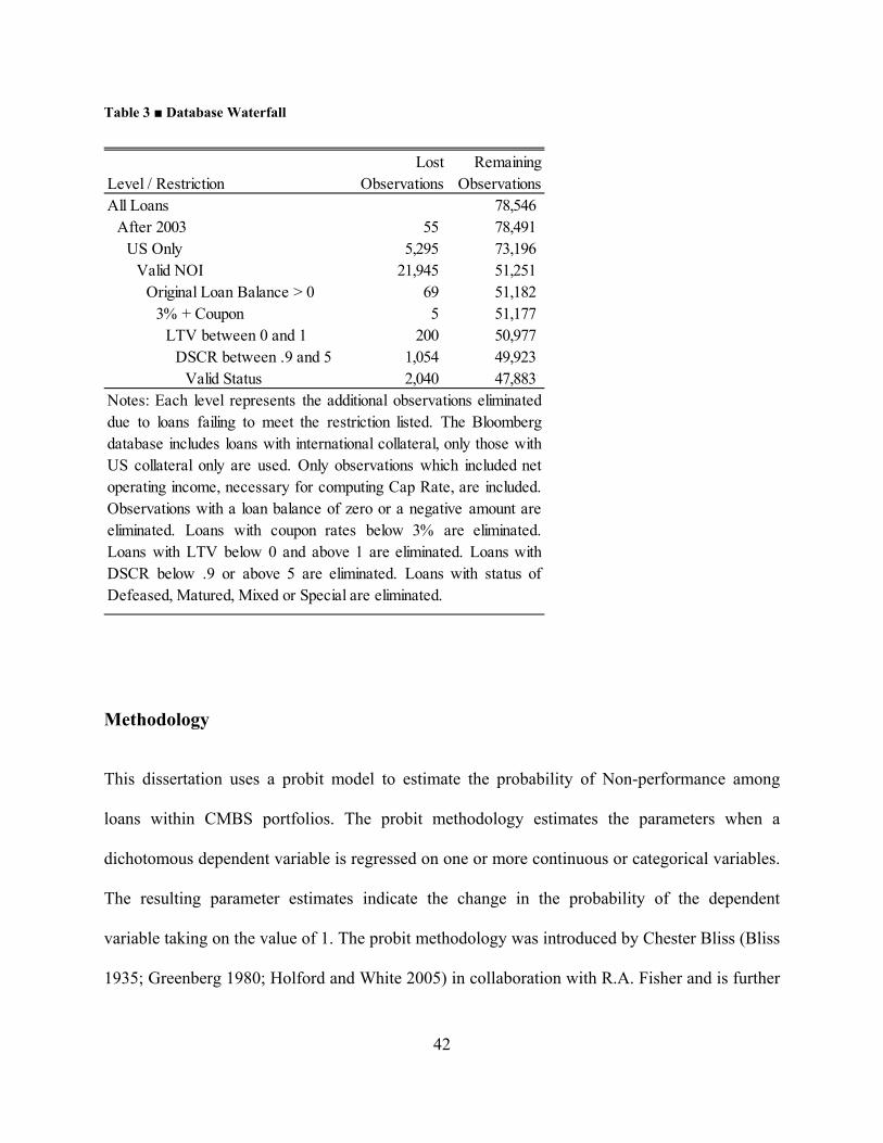
Table 3 ■ Database Waterfall

Methodology

This dissertation uses a probit model to estimate the probability of Non-performance among

loans within CMBS portfolios. The probit methodology estimates the parameters when a

dichotomous dependent variable is regressed on one or more continuous or categorical variables.

The resulting parameter estimates indicate the change in the probability of the dependent

variable taking on the value of 1. The probit methodology was introduced by Chester Bliss (Bliss

1935; Greenberg 1980; Holford and White 2005) in collaboration with R.A. Fisher and is further

Level / RestrictionLost

ObservationsRemaining

ObservationsAll Loans 0 78,546

After 2003 55 78,491 US Only 5,295 73,196

Valid NOI 21,945 51,251 Original Loan Balance > 0 69 51,182

3% + Coupon 5 51,177 LTV between 0 and 1 200 50,977

DSCR between .9 and 5 1,054 49,923 Valid Status 2,040 47,883

Notes: Each level represents the additional observations eliminateddue to loans failing to meet the restriction listed. The Bloombergdatabase includes loans with international collateral, only those withUS collateral only are used. Only observations which included netoperating income, necessary for computing Cap Rate, are included.Observations with a loan balance of zero or a negative amount areeliminated. Loans with coupon rates below 3% are eliminated.Loans with LTV below 0 and above 1 are eliminated. Loans withDSCR below .9 or above 5 are eliminated. Loans with status ofDefeased, Matured, Mixed or Special are eliminated.

43

developed by Finney and Stevens (1948) and Finney (1952). Either the probit or logit approach

may be used in estimating the parameters in such a scenario.

The selection of a particular model, once influenced by computing power, is now typically a

matter of preference (Vincent 2008). Hahn and Sawyer (2005), however, showed that with large

sample sizes and random effects, the probit link function may provide superior results in a

multivariate model than the logit approach, while in the presence of fixed effects or in situations

with extreme values, there may either be no difference or the logit approach may provide better

deviance results. An important assumption in selecting the probit methodology is that the

relationship between the number of CMBS loans defaulting and LTV, DSCR, Debt Yield, and

Cap Rate are normally distributed. To monitor the results for sensitivity to selection of probit

over logit, select tests are also conducted using the logit approach.

The probit methodology was first used for applications such as mortality rates at various

concentrations of drugs in medical studies where a base “mortality correction” must be made if

the mortality in the control group is greater than 10%. For the CMBS loans under study here, no

corollary exists for a no-treatment group, as all loans would have some level of LTV, DSCR,

Debt Yield, and Cap Rate as opposed to a control group in a medical study that may have

received a placebo and thus there would be zero concentration of the drug in question. With this

in mind, there is no need in this study to adjust the base level of mortality (default) as suggested

by Schneider-Orelli (1947).

The probit model takes following form:

Pr (Y = 1 | X) = Φ(X’β), (6)

44

where Pr is the probability and Φ is the cumulative distribution function of the standard normal

distribution. The parameters, denoted by β, are estimated with SAS© 9.2 using the PROBIT

function, which relies on the maximum likelihood procedure.

In the biological sciences, the term LD50 refers to the medial lethal dose of a chemical or a toxic

substance. If one were to consider financial ratios as potentially lethal substances for a CMBS

loan, a certain level of one of these ratios may correspond to a median level of loan default,

controlling for other factors. For example, if the LTV approaches a certain level, one might

expect to see defaults in half of all CMBS loans. Similarly, as the DSCR falls, one would expect

to reach a point where half of all loans default with insufficient cash flow to cover the mortgages.

Centered in the distribution, the formula for LD50, the point at which a financial ratio could be

said to “kill” half of all loans, is the same for both probit and logit models3 (UCLA-ATS 2011).

The formula for LD50 follows the form:

LD50 = - constant/coefficient. (7)

As one moves, however, into the tails of the standard normal and logistic distributions, the probit

and logit values diverge slightly due to differences in the normal and log functions. Substituting

p for the level of the substance (ratio) in question, finding the LD for a probit model requires the

following calculation:

3 For further description of LD50 and LDp calculations with both probit and logit methodologies, see the UCLA Academic Technology Services website at http://www.ats.ucla.edu/stat/mult_pkg/faq/general/ld50.htm

45

Probit LDp = (invnormal (p) - constant)/coefficient. (8)

With the logistic distribution, a logit model uses a different formula to compute the LD levels

with the following formula:

Logit LDp = (log (p/(1-p)) - constant)/coefficient. (9)

The toxic substance metaphor becomes more interesting when one considers medical drug

interactions and how they may lead to increased probability of deadly side effects. Levels of a

substance (ratio in the case of loans) that cause mild reactions among subjects may, when

combined with low levels of another substance (ratio or interest rates), lead to high mortality

rates (loan defaults). For this reason, the models are extended to include interaction terms among

the various loan ratios, and between them and other loan and economic characteristics such as

Cap Rate Spread.

In this research, a probit model measures the impact of the independent variables on the

probability of a CMBS loan having a current status of “Non-performance” as indicated in the

database by the variable “Status.” A new variable labeled “NONP” is created, with all

observations other than those having a Status of Perform or Perform (w)—which indicates that

the loan is performing but has been placed on the servicer’s watch list. Non-performing loans are

assigned a value of 1; Perform and Perform (w) loans are assigned a value of 0.

The equation below provides an example of the approach followed in this dissertation. In this

example, only one of the ratio measures (LTV or DSCR) is included in the model along with the

natural log of loan size, recent S&P index returns, market interest rate, the spread between the

market rate and the loan rate, the spread between the Cap Rate and the loan rate, as well as

46

indicator variables for amortization type, interest rate type, state, loan originator, and property

type. These variables are all described later in the Data and Methodology section. Other models

will incorporate combinations of the ratio measures, as well as two-stage equations, and split

samples with the goal of testing the robustness of the results.

NONP 10

= f (LTV or DSCR, LnSIZE, SPY, INT, CPNSPRD, CAPSPRD, AMORTi , RATEi,

STATEi, ORIGi, PTYPEi) (10)

Hypothesis 1

Hypothesis 1 tests the theory that the spread between the rate of interest on the loan and the Cap

Rate at the time of origination (Cap Rate Spread – CAPSPRD) is negatively related to Non-

performance. This theory would predict that as the cushion between the loan interest rate and the

Cap Rate on the property increases, the incidence of Non-performance would drop. Conversely,

the theory would predict that loans underwritten with a very low margin between the loan

interest rate and the return on the property are at greater risk of Non-performance and ultimately

of default. In testing Hypothesis 1, probit model parameters are estimated with the equation:

Pr (NONP = 1 | X) = Φ(X’β), (11)

where X’ is a vector of one of several combinations of the following covariates:

Loan to Value—this variable (LTV) is the ratio of the original loan balance to the value of the

property. Lenders typically require between .75-.85 for project approval, though it was not

uncommon during the mid-2000s for LTVs to be much higher, often approaching 1.0 and

sometimes moving beyond.

47

Debt Service Coverage Ratio—this variable (DSCR) is the ratio of a borrower’s (project’s)

annual net operating income to the annual debt service requirement including both principal and

interest. Lenders generally require ratios between 1.1-1.25 for project approval.

Loan Size—the natural log of original loan balance in dollars (LnSIZE) for each observation.

This variable is intended to capture loan performance risks and underwriting behavior

differences related to the size of the project and loan amount originated.

Equity Market Returns—the yield on the S&P Index for the prior 3-month period. This variable

is intended to capture the effects of the broad U.S. stock market on CMBS loan underwriting

behavior. Recent gains or losses in the stock markets may differentially affect the underwriting

decisions due to changed demand for CMBS products, return expectations, and sentiment. S&P

Yield (SPY) measures the change in percent of the S&P Index for the three month period

preceding the origination of the observation.

Interest Rate—the rate of the 10-Year constant maturity Treasury at the time of loan origination.

This data series is retrieved from the U.S. Treasury website and is matched with the Bloomberg

loan data using the date of origination for the loan and the date provided in the daily rate file.

Interest Rate (INT) measures the market yield in percent per year on 10-Year constant-maturity

Treasury securities, quoted on investment basis.

Origination Volume—the number of CMBS loans originated in the 12 months prior to the

origination of the observation. This variable is scaled by a factor of .01 in order to aid the

presentation and interpretation of the coefficient estimates. Origination (DEALS) measures the

number of CMBS loan originations in the last 12 months, divided by 100.

48

Coupon Spread (CPNSPRD) – the difference between the coupon interest rate on the loan at

origination (NETCPN) and the market yield on 10-Year Treasuries on the date of loan

origination (INT). In theory, a commercial loan coupon rate should represent the investor’s

required rate of return, i.e., the discount rate utilized in determining the present value of the

loan’s cash flows. The difference between the prevailing interest rates and the coupon rate on a

commercial mortgage should represent the originator’s assessment of default risk for the loan

relative to alternative investments and may serve as a normalized measure of loan risk. As the

LTV on a loan rises and the DSCR on a loan falls, one would expect the coupon spread

(CPNSPRD) to rise accordingly. As a result, multicollinearity is to be expected among these

variables. Assuming, however, that underwriters consider other, perhaps unmeasured, factors in

addition to LTV and DSCR in making origination judgments, the net coupon rate may capture

attempts to price these risks into the loan.

Cap Rate Spread—this variable (CAPSPRD) is the spread between the coupon rate of the loan

and the Cap Rate, the ratio of the net operating income of the property serving as collateral for

the total value of the project. Cap Rate, also called the overall capitalization rate, is used in

evaluating commercial real estate and represents an unleveraged rate of return on the project.

State — The largest group of the CMBS loans were originated for property in the state of

California (10,576) while Vermont saw only 68 loans originated during the sample period. Due

to differing economic conditions, regulatory environments, and business cycles, controlling for

geography is an important consideration when estimating the factors affecting CMBS loan

performance. In order to control for these geographic conditions, indicator variables are created

49

for each state plus Washington, DC. STATEi indicator variables represent the State where the

loan collateral is located.

Rate Type — The CMBS loan underwriters shifted risks to the borrower in varying degrees by

offering different fixed and adjustable rate types. Like the amortization, the type of rate may

reflect a bank’s assessment of the risk and would be an important factor in understanding and

comparing the actual rate set on the loan. For example, a rate of 5% may be at the same time

high for an adjustable loan and low for a fixed rate loan. Example rate types include fixed and

those indexed to LIBOR, EURIBOR, prime, COFI, and U.S. Treasuries. RATEi indicator

variables represent the rate type of the loan.

Amortization Type —All things being equal, the amortization type for a loan may reflect a

bank’s assessment of the risk and would be an important factor in understanding and comparing

the actual rate set on the loan. Example amortization types include fully amortizing, interest

only, balloon amortizing, partial interest only, and mixed. AMORTi indicator variables represent

the amortization type of the loan.

Property Type—the building serving as collateral for each CMBS loan may be in one of several

different property-type categories including office, retail, industrial, and multifamily. Because

each of these property types may be subject to differing sensitivities to the variables of interest in

this study, they are incorporated into the model to control for this possibility. Over the last

twenty years, in addition to periods of increasing and decreasing interest rates, there have also

been periods or cycles of greater CMBS loan activity in different commercial property types.

During some periods, for example, there was a much larger proportion of loan originations in

multifamily dwellings, while other periods saw more activity in office or other property types.

50

Different property types may be more or less sensitive to varying economic conditions and thus

the loans underwritten to fund projects in different property categories may vary in their

probability of default. Further, the likelihood that loans in different property types will default

may vary according to the interest rate environment during which they were originated. One

motivation for this extension is the observation that some periods had originations that were

almost exclusively in one property type while other periods had mixtures of different property

types. Ignoring this important variable may introduce a missing variable bias and lead to

erroneous conclusions regarding other variables that tend to vary over time. PTYPEi indicator

variables represent the predominant property type serving as collateral for the loan.

Originator—the financial institution responsible for underwriting and originating the loan. The

institutions rely upon the various ratios, industry knowledge, proprietary information, and

personal relationships to assess risk and price the loan terms. The real estate literature proposes

other variables such as recent negative stock performance of loan originators, which may prompt

more risky underwriting in order to generate fees. Additionally, the history of the CMBS market

includes large swings in the economy and regulatory changes which may have altered the

behavior of loan originators in ways that precipitated the troubles that followed.

Some CMBS loan underwriters, such as U.S. conduits and foreign entities, have experienced

high levels of mortgage defaults while others, such as insurance companies, have fared better

despite intense economic pressure on the industry as a whole during the recent financial crisis

(Black, Chu, Cohen, and Nichols 2011). Though some firms take a more aggressive approach

with respect to LTV and DSCR standards, their methods may also be influenced by such factors

as firm culture, incentive structures, and governance characteristics. This conjecture provides

51

motivation to test for originating firm variables that go beyond the traditional ratio tests in

predicting CMBS loan default. Therefore, in this dissertation, the analysis is extended by

incorporating indicator variables for each CMBS loan originator. ORIGi indicator variables

represent the firm originating the CMBS loan.

With the full list of variables, the model tested under Hypothesis 1 may be presented as:

NONP 10

= f (LTV or DSCR, LnSIZE, SPY, INT,DEALS, CPNSPRD, CAPSPRD, AMORTi ,

RATEi,STATEi, ORIGi, PTYPEi) (12)

Hypothesis 2

In testing Hypothesis 2, estimates are calculated using the prior probit model parameters with the

sample divided into two distinct groups: Fixed-Rate Balloon loans and all other loans. As with

the prior model, the dependent variable is Non-performance and X’ is a vector of a covariates,

including Cap Rate Spread as the variable of interest. The remaining variables used in the model

to test Hypothesis 2 remain unchanged from the prior model, resulting in the following full

model for Fixed Rate Balloon Loans:

NONP 10

= f (LTV or DSCR, LnSIZE, SPY, INT,DEALS, CPNSPRD, CAPSPRD, RATEi,

STATEi, ORIGi, PTYPEi) (13)

Equation (13) is estimated for Fixed Rate Balloon Loans only. Similarly, the model used to

estimate the relationships for all other loans is specified as follows:

NONP 10

= f (LTV or DSCR, LnSIZE, SPY, INT,DEALS, CPNSPRD, CAPSPRD, AMORTi ,

RATEi,STATEi, ORIGi, PTYPEi) (14)

52

The sample used to estimate Equation (14) excludes all Fixed Rate Balloon Loans.

Hypothesis 3

Hypothesis 3 tests the value of a Cap Rate Spread underwriting standard above and beyond the

result of using LTV and DSCR standards. Using a LTV cutoff of .8 and a DSCR cutoff of 1.25,

only loans which would pass underwriter scrutiny under both of these standards are considered in

using a model to estimate the parameters for Cap Rate Spread and the other covariates.

Consistent with the model under Hypothesis 2, the model used to estimate the relationships

tested under Hypothesis 3 is specified as follows:

NONP 10

= f (LTV or DSCR, LnSIZE, SPY, INT,DEALS, CPNSPRD, CAPSPRD, AMORTi ,

RATEi,STATEi, ORIGi, PTYPEi) (15)

Equation (15) is estimated for only loans with LTV less than .8 and DSCR greater than 1.25 at the

time of origination. As with the results from the prior probit models, the coefficient for Cap Rate

Spread in this model will estimate the z-score or change in probability of Non-performance that

is associated with a one-unit change in Cap Rate Spread. A significant negative relationship

would support Hypothesis 3 indicating that Cap Rate Spread provides additional information

even among loans considered safe by LTV and DSCR standards.

Hypothesis 4

The fourth and final Hypothesis contends that an underwriting standard utilizing Cap Rate

Spread may help reduce the level of non-performing loans. While the selection of a floor beyond

which loans would not be originated is somewhat arbitrary and subject to manipulation, the

53

process illustrates the outcome potential of such an exercise. Underwriters of different firms face

a wide range of investment objectives, loan approval pressures, system sophistication, and other

underwriting standards. Each underwriter may choose to set their standards for LTV, DSCR, and

Cap Rate Spread according to their individual firm’s appetite for risk, the expected proportion of

loans to be held on the company’s own books, or other criteria. For this numerical model, the

“safe” sample used to test Hypothesis 3 is again chosen to test further restrictive criteria for

approving loans: a minimum Cap Rate Spread of 1%. Loans below this floor would not be

approved even though they may have passed the LTV and DSCR requirements previously

described. The outcome of this process will be a new set of loans which would have met all three

standards. The remaining loans are those which would have passed the LTV and DSCR tests but

failed the Cap Rate Spread test.

Evaluating each of these sets provides some interesting, though admittedly limited, insights into

how a Cap Rate Spread-based underwriting rule would have performed through the recent

financial crisis. Among the loans that would have been declined are many which are still

performing today. Similarly, the set of loans which passed all three tests includes many non-

performing loans. These two groups of loans-performing loans which would have never been

originated and non-performing loans which passed all three ratio tests-are similar to the false

positive (Type I) and false negative (Type II) errors reported with other forms of testing and

analysis. It is important to point out that this numerical modeling approach is intended to simply

provide insight into how Cap Rate Spread underwriting criteria may be incorporated into a

comprehensive underwriting process. The error rates associated with the different sets of rules

54

will be reported along with the changes to the quantities of loans originated throughout the

sample period.

Robustness Checks

In addition to the primary methods outlined to test the hypotheses, several robustness checks will

be conducted to test for sensitivity to choices made as part the research design. First, selected

probit model specifications will also be conducted using a two-stage regression methodology

designed to correct for possible endogeneity between the pricing of the loan (NETCPN) and the

traditional ratios LTV and DSCR. If these factors are jointly determined in a process which

trades off values of these against each other, results which assume their independence will be

biased. Because Cap Rate Spread is calculated using Net Coupon Rate, endogeneity with LTV

and/or DSCR would bias the estimated coefficients of the relationships between these right hand

side variables and Non-performance. The first stage of the two-stage model will estimate the Net

Coupon Rate of the loan using some overlapping variables along with a set of instrumental

variables which identify the equation. The first stage of the model is as follows:

NETCPN = f (LTV, DSCR, INT, YQi, STATEi, RATEi, AMORTi, PTYPEi, ORIGi). (12)

The predicted net coupon rate (PREDNETCPN) for each observation is used to calculate a

predicted Cap Rate Spread where:

PREDCAPSPRD = CAPRT- PREDNETCPN. (13)

55

In the second stage of the model, the CAPSPRD used in prior models is replaced by the value

derived from the predicted net coupon rate (PREDNETCPN). The resulting equation is as

follows:

NONP 10

= f (LTV or DSCR, LnSIZE, SPY, INT, DEALS, CPNSPRD, PREDCAPSPRD, AMORTi ,

RATEi,STATEi, ORIGi, PTYPEi) (18)

An additional concern in estimating the models in this dissertation is the assumption that the

binary relationship between the right hand side variables and the incidence of Non-performance

follows a standard normal distribution. It may also be the case that a logit model, which assumes

a logistic distribution, better fits the true relationships. To test this assumption, select models are

modified and estimated using a binary logistic method to test for sensitivity to the distribution

assumption. Parameter estimates, direction and significance are expected to be similar to those

estimated using probit models.

56

CHAPTER FOUR – ANALYSIS OF RESULTS

Descriptive Statistics

In order to provide a broad appreciation for the CMBS loan sample, basic statistical measures are

reported for the variables used in this dissertation including minimum value, maximum value,

mean, and standard deviation. Additionally, tables separating the sample by values for each of

the dummy variables describe the size of each category and the mean values for the other key

variables including LTV, DSCR and Cap Rate. Analyzing the distribution of the sample

categorically reveals likely drivers of heterogeneity within the sample and provides a rationale

for including the respective control variables for factors such as the regional variation captured

by using STATEi indicator variables. The first table of descriptive statistics, Table 4, provides

summary statistics describing the variables of interest for the full date range of the database –

January 1993 to September 2011.

The size of loans underwritten for CMBS distribution varies considerably with an average loan

amount of $12.4 million and a standard deviation of $43.2 million. The sample of loans includes

several very large loans such as the Equity Office Portfolio at $6.87 billion, the Hilton

Worldwide Portfolio at $2.87 billion, the Extended Stay Hotel Portfolio at $2.0 billion,

Rockefeller Center at $1.69 billion, the largest of the Peter Cooper Village/Stuyvesant Town

loans at $1.5 billion, and the La Quinta/Baymont Portfolio at $1.44 billion. Rather than remove

these potential outliers, the log of loan size (LnSIZE) is used to better model the likely

relationship between loan size and Non-performance (NONP).

57

Interest rates (NETCPN) charged on loans in the final sample range from a low of 2.65% to a

high of 15% with a mean of 6.02% and a fairly tight distribution with a standard deviation of

only .88%. The LTV ratios at the securitization cutoff date in the full database (not reported in

Table 4) range from very small (.005) to very large (2.62) with a mean of .670. The database also

included observations with LTVs of 0 despite data on these observations for loan amount and

recent valuations. Observations where LTV is 0 or greater than 1 are eliminated from the sample.

90% of the observations in the sample fall between .39 and .80 with only 1% above .85. After the

elimination of the observations with LTV at or below 0 and the other sample trimming measures,

minimum value for LTV is .02, the maximum is 1.0 and the mean rises to .68 with a standard

deviation of .12.

Debt service coverage ratios at cutoff in the full sample (not reported in Table 4) range from

negative values as low as -.18 to extremely large (topping out at 136) with a mean of 1.63.

Values below .9 and above 5 are eliminated. Ninety percent of the observations have DSCR

between 1.06 and 2.35. 98% fall between 1.02 and 7.23. After eliminating the extreme values,

DSCR for the final sample ranges from a low of .91 to a high of 5.00 with a mean of 1.46 and a

standard deviation of .39. During the sample period the rates on 10-Year U.S. Treasuries ranged

from a high of 7.92% in late 1994 to a low of 2.02% in late 2011. The mean interest rate at the

time of origination for all observations in the sample is 4.49%.

The dependent variable in the empirical analysis is loan Non-performance (NONP). The mean

for this variable across all observations is .21 and is a grouping of loan status indicators which all

relate to a condition of Non-performance. The categories which are grouped in to the Non-

performance category include delinquent, in foreclosure, grace, late, non-performing, and REO.

58

Those loans with a current status of defeased, matured, mixed, or special are not included in the

sample.

The difference between the coupon rate of the loan (NETCPN) and the 10-Year Treasury note at

the time of origination (INT), Coupon Spread (CPNSPRD), ranges from -1.92% to a high of

11.63% with a mean of 1.53% and a standard deviation of .80%. This measure is indicative of

the bank’s relative yield on the loan at the time of origination. The difference between the

property Cap Rate and the coupon rate (NETCPN) is CAPSPRD, ranging from -10% to a high of

392% with a mean of 2% and a standard deviation of 9%. The measure relating to recent stock

market returns is the 12 month change in the S&P index as a percentage. With a large proportion

of values negative, the variable used the empirical tests is increased by 1 yielding all positive

values with a mean of 1.12 (12% increase in the S&P index for the prior 12 months), a minimum

of .47, a maximum of 1.62 and a standard deviation of .15.

A measure of recent CMBS origination activity is also incorporated into the analysis to account

for the possibility that high or low volume may affect the origination decision process as

underwriters are either rushed or have more time for due diligence. Periods of strong origination

activity may lead to increased competition among underwriters attempting to fill bond pools with

loans. The measure used is the number of CMBS loans originated in the period 12 months prior

to the origination date of the observation (DEALS). The value is then scaled by dividing by 100.

The mean value is .73 (73 loans originated in the 12 months prior to the origination date of the

observation), the minimum is 0, the maximum is 5.37 (537 loans) and the standard deviation is

.92 (92 loans).

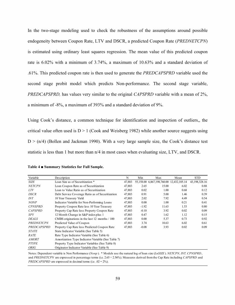
59

In the two-stage modeling used to check the robustness of the assumptions around possible

endogeneity between Coupon Rate, LTV and DSCR, a predicted Coupon Rate (PREDNETCPN)

is estimated using ordinary least squares regression. The mean value of this predicted coupon

rate is 6.02% with a minimum of 3.74%, a maximum of 10.63% and a standard deviation of

.61%. This predicted coupon rate is then used to generate the PREDCAPSPRD variable used the

second stage probit model which predicts Non-performance. The second stage variable,

PREDCAPSPRD, has values very similar to the original CAPSPRD variable with a mean of 2%,

a minimum of -8%, a maximum of 393% and a standard deviation of 9%.

Using Cook’s distance, a common technique for identification and inspection of outliers,, the

critical value often used is D > 1 (Cook and Weisberg 1982) while another source suggests using

D > (n/4) (Bollen and Jackman 1990). With a very large sample size, the Cook’s distance test

statistic is less than 1 but more than n/4 in most cases when evaluating size, LTV, and DSCR.

Table 4 ■ Summary Statistics for Full Sample.

Variable Description N Min Max Mean STDSIZE Loan Size as of Securitization * 47,883 55,158.00 6,867,198,760.00 12,432,105.14 43,198,328.16NETCPN Loan Coupon Rate as of Securitization 47,883 2.65 15.00 6.02 0.88LTV Loan to Value Ratio as of Securitization 47,883 0.02 1.00 0.68 0.12DSCR Debt Service Coverage Ratio as of Securitization 47,883 0.91 5.00 1.46 0.39INT 10 Year Treasury Yield 47,883 2.02 7.92 4.49 0.54NONP Indicator Variable for Non-Performing Loans 47,883 0.00 1.00 0.21 0.41CPNSPRD Property Coupon Rate less 10 Year Treasury 47,883 -1.92 11.63 1.53 0.80CAPSPRD Property Cap Rate less Property Coupon Rate 47,883 -0.10 3.92 0.02 0.09SPY 12 Month Change in S&P index plus 1 47,883 0.47 1.62 1.12 0.15DEALS CMBS originations in the last 12 months / 100 47,883 0.00 5.37 0.73 0.92PREDNETCPN Predicted Value of Coupon 47,883 3.74 10.63 6.02 0.61PREDCAPSPRD Property Cap Rate less Predicted Coupon Rate 47,883 -0.08 3.93 0.02 0.09STATE State Indicator Variable (See Table 5)RATE Rate Type Indicator Variable (See Table 6)AMORT Amortization Type Indicator Variable (See Table 7)PTYPE Property Type Indicator Variables (See Table 8)ORIG Originator Indicator Variable (See Table 9)

Notes: Dependent variable is Non Performance (Nonp ). * Models use the natural log of loan size (LnSIZE ). NETCPN, INT, CPNSPRD , and PREDNETCPN are expressed in percentage terms (i.e. 2.65 = 2.56%). Measures derived from the Cap Rate including CAPSPRD and PREDCAPSPRD are expressed in decimal terms (i.e. .02 = 2%).

60

In order to control for geographic effects, dummy variables for the U.S. State have been included

throughout into the empirical analysis. Several of the variables of interest fluctuate considerably

by State and support the work of prior researchers who considered regional differences when

attempting to understand CMBS loan performance. The state with the largest number of

observations is California with 8,209 loans originated, 17.14% of the sample. For the empirical

analysis, California is the excluded case and thus sets the model baseline. Table 5 presents the

full list of 50 states plus the District of Columbia and the means and standard deviations for each

of the key variables of interest: Non-performance, LTV, DSCR, and Cap Rate. As expected,

states with below average rates of Non-performance appear to be associated with lower LTVs

and higher DSCRs. California, for example has a .17 rate of Non-performance, average LTV is

.63 and the average DSCR is 1.48. This compares to Arizona, 3% of the sample, with a .30 rate

of Non-performance, average LTV is .69 and the average DSCR is 1.42. Incorporating STATEi

dummy variables into the empirical analysis controls for fixed effects attributable to the State

where the property as collateral for the loan is geographically located.

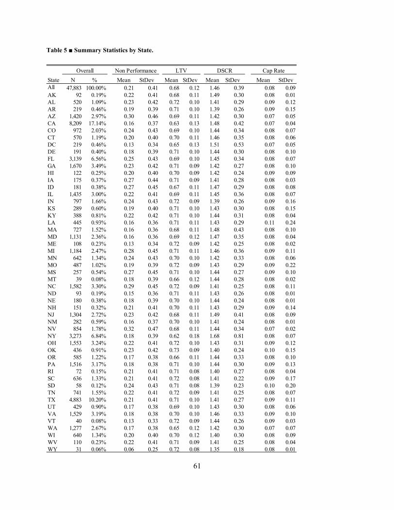
61

Table 5 ■ Summary Statistics by State.

State N % Mean StDev Mean StDev Mean StDev Mean StDevAll 47,883 100.00% 0.21 0.41 0.68 0.12 1.46 0.39 0.08 0.09AK 92 0.19% 0.22 0.41 0.68 0.11 1.49 0.30 0.08 0.01AL 520 1.09% 0.23 0.42 0.72 0.10 1.41 0.29 0.09 0.12AR 219 0.46% 0.19 0.39 0.71 0.10 1.39 0.26 0.09 0.15AZ 1,420 2.97% 0.30 0.46 0.69 0.11 1.42 0.30 0.07 0.05CA 8,209 17.14% 0.16 0.37 0.63 0.13 1.48 0.42 0.07 0.04CO 972 2.03% 0.24 0.43 0.69 0.10 1.44 0.34 0.08 0.07CT 570 1.19% 0.20 0.40 0.70 0.11 1.46 0.35 0.08 0.06DC 219 0.46% 0.13 0.34 0.65 0.13 1.51 0.53 0.07 0.05DE 191 0.40% 0.18 0.39 0.71 0.10 1.44 0.30 0.08 0.10FL 3,139 6.56% 0.25 0.43 0.69 0.10 1.45 0.34 0.08 0.07GA 1,670 3.49% 0.23 0.42 0.71 0.09 1.42 0.27 0.08 0.10HI 122 0.25% 0.20 0.40 0.70 0.09 1.42 0.24 0.09 0.09IA 175 0.37% 0.27 0.44 0.71 0.09 1.41 0.28 0.08 0.03ID 181 0.38% 0.27 0.45 0.67 0.11 1.47 0.29 0.08 0.08IL 1,435 3.00% 0.22 0.41 0.69 0.11 1.45 0.36 0.08 0.07IN 797 1.66% 0.24 0.43 0.72 0.09 1.39 0.26 0.09 0.16KS 289 0.60% 0.19 0.40 0.71 0.10 1.43 0.30 0.08 0.15KY 388 0.81% 0.22 0.42 0.71 0.10 1.44 0.31 0.08 0.04LA 445 0.93% 0.16 0.36 0.71 0.11 1.43 0.29 0.11 0.24MA 727 1.52% 0.16 0.36 0.68 0.11 1.48 0.43 0.08 0.10MD 1,131 2.36% 0.16 0.36 0.69 0.12 1.47 0.35 0.08 0.04ME 108 0.23% 0.13 0.34 0.72 0.09 1.42 0.25 0.08 0.02MI 1,184 2.47% 0.28 0.45 0.71 0.11 1.46 0.36 0.09 0.11MN 642 1.34% 0.24 0.43 0.70 0.10 1.42 0.33 0.08 0.06MO 487 1.02% 0.19 0.39 0.72 0.09 1.43 0.29 0.09 0.22MS 257 0.54% 0.27 0.45 0.71 0.10 1.44 0.27 0.09 0.10MT 39 0.08% 0.18 0.39 0.66 0.12 1.44 0.28 0.08 0.02NC 1,582 3.30% 0.29 0.45 0.72 0.09 1.41 0.25 0.08 0.11ND 93 0.19% 0.15 0.36 0.71 0.11 1.43 0.26 0.08 0.01NE 180 0.38% 0.18 0.39 0.70 0.10 1.44 0.24 0.08 0.01NH 151 0.32% 0.21 0.41 0.70 0.11 1.43 0.29 0.09 0.14NJ 1,304 2.72% 0.23 0.42 0.68 0.11 1.49 0.41 0.08 0.09NM 282 0.59% 0.16 0.37 0.70 0.10 1.41 0.24 0.08 0.01NV 854 1.78% 0.32 0.47 0.68 0.11 1.44 0.34 0.07 0.02NY 3,273 6.84% 0.18 0.39 0.62 0.18 1.68 0.81 0.08 0.07OH 1,553 3.24% 0.22 0.41 0.72 0.10 1.43 0.31 0.09 0.12OK 436 0.91% 0.23 0.42 0.73 0.09 1.40 0.24 0.10 0.15OR 585 1.22% 0.17 0.38 0.66 0.11 1.44 0.33 0.08 0.10PA 1,516 3.17% 0.18 0.38 0.71 0.10 1.44 0.30 0.09 0.13RI 72 0.15% 0.21 0.41 0.71 0.08 1.40 0.27 0.08 0.04SC 636 1.33% 0.21 0.41 0.72 0.08 1.41 0.22 0.09 0.17SD 58 0.12% 0.24 0.43 0.71 0.08 1.39 0.23 0.10 0.20TN 741 1.55% 0.22 0.41 0.72 0.09 1.41 0.25 0.08 0.07TX 4,883 10.20% 0.21 0.41 0.71 0.10 1.41 0.27 0.09 0.11UT 429 0.90% 0.17 0.38 0.69 0.10 1.43 0.30 0.08 0.06VA 1,529 3.19% 0.18 0.38 0.70 0.10 1.46 0.33 0.09 0.10VT 40 0.08% 0.13 0.33 0.72 0.09 1.44 0.26 0.09 0.03WA 1,277 2.67% 0.17 0.38 0.65 0.12 1.42 0.30 0.07 0.07WI 640 1.34% 0.20 0.40 0.70 0.12 1.40 0.30 0.08 0.09WV 110 0.23% 0.22 0.41 0.71 0.09 1.41 0.25 0.08 0.04WY 31 0.06% 0.06 0.25 0.72 0.08 1.35 0.18 0.08 0.01

Overall Cap RateDSCRLTVNon Performance

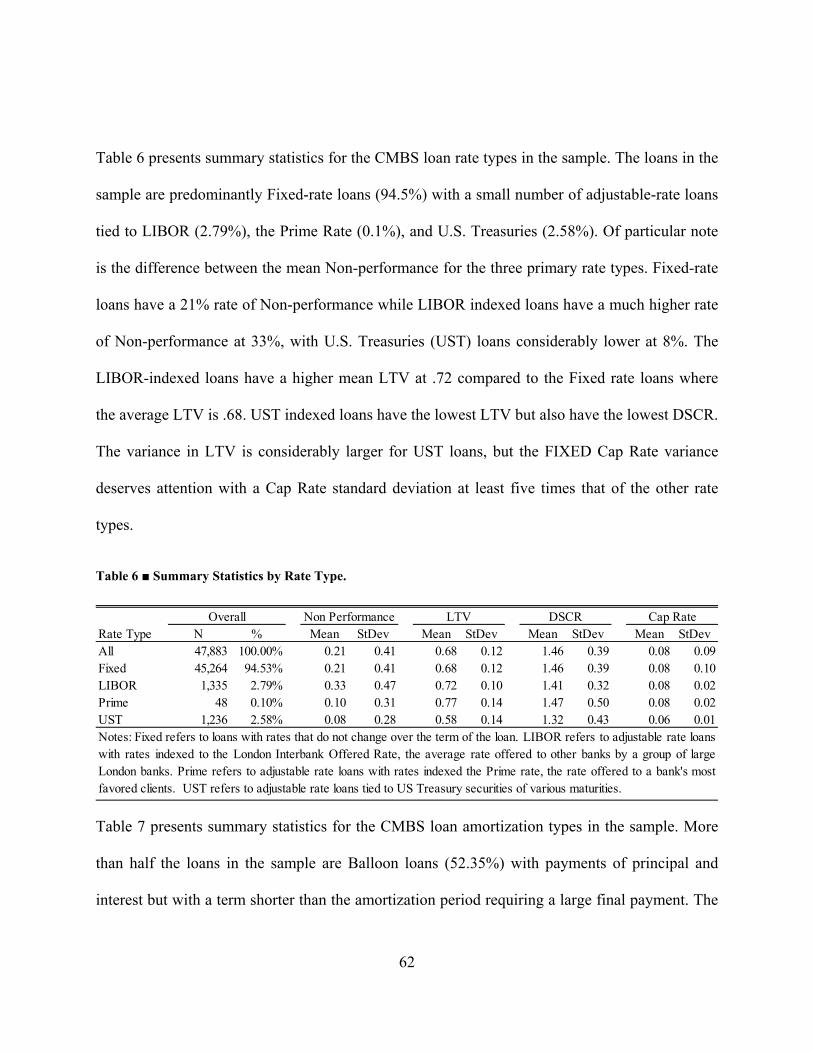
62

Table 6 presents summary statistics for the CMBS loan rate types in the sample. The loans in the

sample are predominantly Fixed-rate loans (94.5%) with a small number of adjustable-rate loans

tied to LIBOR (2.79%), the Prime Rate (0.1%), and U.S. Treasuries (2.58%). Of particular note

is the difference between the mean Non-performance for the three primary rate types. Fixed-rate

loans have a 21% rate of Non-performance while LIBOR indexed loans have a much higher rate

of Non-performance at 33%, with U.S. Treasuries (UST) loans considerably lower at 8%. The

LIBOR-indexed loans have a higher mean LTV at .72 compared to the Fixed rate loans where

the average LTV is .68. UST indexed loans have the lowest LTV but also have the lowest DSCR.

The variance in LTV is considerably larger for UST loans, but the FIXED Cap Rate variance

deserves attention with a Cap Rate standard deviation at least five times that of the other rate

types.

Table 6 ■ Summary Statistics by Rate Type.

Table 7 presents summary statistics for the CMBS loan amortization types in the sample. More

than half the loans in the sample are Balloon loans (52.35%) with payments of principal and

interest but with a term shorter than the amortization period requiring a large final payment. The

Rate Type N % Mean StDev Mean StDev Mean StDev Mean StDevAll 47,883 100.00% 0.21 0.41 0.68 0.12 1.46 0.39 0.08 0.09Fixed 45,264 94.53% 0.21 0.41 0.68 0.12 1.46 0.39 0.08 0.10LIBOR 1,335 2.79% 0.33 0.47 0.72 0.10 1.41 0.32 0.08 0.02Prime 48 0.10% 0.10 0.31 0.77 0.14 1.47 0.50 0.08 0.02UST 1,236 2.58% 0.08 0.28 0.58 0.14 1.32 0.43 0.06 0.01Notes: Fixed refers to loans with rates that do not change over the term of the loan. LIBOR refers to adjustable rate loanswith rates indexed to the London Interbank Offered Rate, the average rate offered to other banks by a group of largeLondon banks. Prime refers to adjustable rate loans with rates indexed the Prime rate, the rate offered to a bank's mostfavored clients. UST refers to adjustable rate loans tied to US Treasury securities of various maturities.

Overall Non Performance LTV DSCR Cap Rate

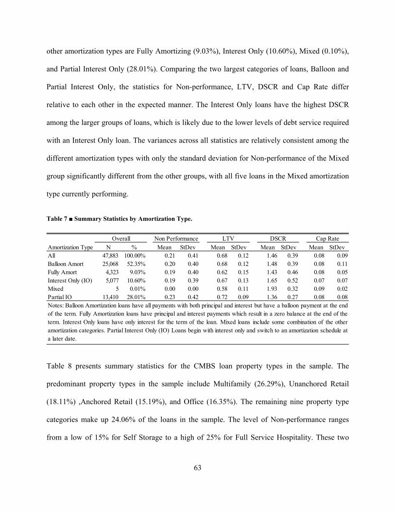
63

other amortization types are Fully Amortizing (9.03%), Interest Only (10.60%), Mixed (0.10%),

and Partial Interest Only (28.01%). Comparing the two largest categories of loans, Balloon and

Partial Interest Only, the statistics for Non-performance, LTV, DSCR and Cap Rate differ

relative to each other in the expected manner. The Interest Only loans have the highest DSCR

among the larger groups of loans, which is likely due to the lower levels of debt service required

with an Interest Only loan. The variances across all statistics are relatively consistent among the

different amortization types with only the standard deviation for Non-performance of the Mixed

group significantly different from the other groups, with all five loans in the Mixed amortization

type currently performing.

Table 7 ■ Summary Statistics by Amortization Type.

Table 8 presents summary statistics for the CMBS loan property types in the sample. The

predominant property types in the sample include Multifamily (26.29%), Unanchored Retail

(18.11%) ,Anchored Retail (15.19%), and Office (16.35%). The remaining nine property type

categories make up 24.06% of the loans in the sample. The level of Non-performance ranges

from a low of 15% for Self Storage to a high of 25% for Full Service Hospitality. These two

Amortization Type N % Mean StDev Mean StDev Mean StDev Mean StDevAll 47,883 100.00% 0.21 0.41 0.68 0.12 1.46 0.39 0.08 0.09Balloon Amort 25,068 52.35% 0.20 0.40 0.68 0.12 1.48 0.39 0.08 0.11Fully Amort 4,323 9.03% 0.19 0.40 0.62 0.15 1.43 0.46 0.08 0.05Interest Only (IO) 5,077 10.60% 0.19 0.39 0.67 0.13 1.65 0.52 0.07 0.07Mixed 5 0.01% 0.00 0.00 0.58 0.11 1.93 0.32 0.09 0.02Partial IO 13,410 28.01% 0.23 0.42 0.72 0.09 1.36 0.27 0.08 0.08Notes: Balloon Amortization loans have all payments with both principal and interest but have a balloon payment at the endof the term. Fully Amortization loans have principal and interest payments which result in a zero balance at the end of theterm. Interest Only loans have only interest for the term of the loan. Mixed loans include some combination of the otheramortization categories. Partial Interest Only (IO) Loans begin with interest only and switch to an amortization schedule ata later date.

Overall Non Performance LTV DSCR Cap Rate

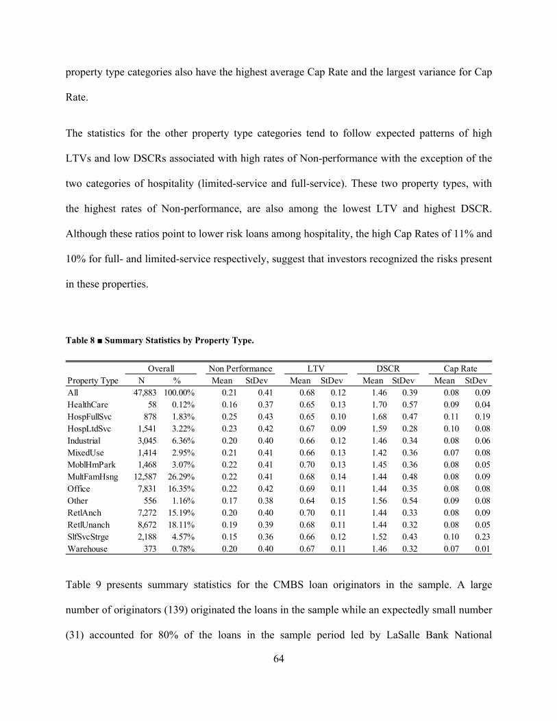
64

property type categories also have the highest average Cap Rate and the largest variance for Cap

Rate.

The statistics for the other property type categories tend to follow expected patterns of high

LTVs and low DSCRs associated with high rates of Non-performance with the exception of the

two categories of hospitality (limited-service and full-service). These two property types, with

the highest rates of Non-performance, are also among the lowest LTV and highest DSCR.

Although these ratios point to lower risk loans among hospitality, the high Cap Rates of 11% and

10% for full- and limited-service respectively, suggest that investors recognized the risks present

in these properties.

Table 8 ■ Summary Statistics by Property Type.

Table 9 presents summary statistics for the CMBS loan originators in the sample. A large

number of originators (139) originated the loans in the sample while an expectedly small number

(31) accounted for 80% of the loans in the sample period led by LaSalle Bank National

Property Type N % Mean StDev Mean StDev Mean StDev Mean StDevAll 47,883 100.00% 0.21 0.41 0.68 0.12 1.46 0.39 0.08 0.09HealthCare 58 0.12% 0.16 0.37 0.65 0.13 1.70 0.57 0.09 0.04HospFullSvc 878 1.83% 0.25 0.43 0.65 0.10 1.68 0.47 0.11 0.19HospLtdSvc 1,541 3.22% 0.23 0.42 0.67 0.09 1.59 0.28 0.10 0.08Industrial 3,045 6.36% 0.20 0.40 0.66 0.12 1.46 0.34 0.08 0.06MixedUse 1,414 2.95% 0.21 0.41 0.66 0.13 1.42 0.36 0.07 0.08MoblHmPark 1,468 3.07% 0.22 0.41 0.70 0.13 1.45 0.36 0.08 0.05MultFamHsng 12,587 26.29% 0.22 0.41 0.68 0.14 1.44 0.48 0.08 0.09Office 7,831 16.35% 0.22 0.42 0.69 0.11 1.44 0.35 0.08 0.08Other 556 1.16% 0.17 0.38 0.64 0.15 1.56 0.54 0.09 0.08RetlAnch 7,272 15.19% 0.20 0.40 0.70 0.11 1.44 0.33 0.08 0.09RetlUnanch 8,672 18.11% 0.19 0.39 0.68 0.11 1.44 0.32 0.08 0.05SlfSvcStrge 2,188 4.57% 0.15 0.36 0.66 0.12 1.52 0.43 0.10 0.23Warehouse 373 0.78% 0.20 0.40 0.67 0.11 1.46 0.32 0.07 0.01

Overall Non Performance LTV DSCR Cap Rate

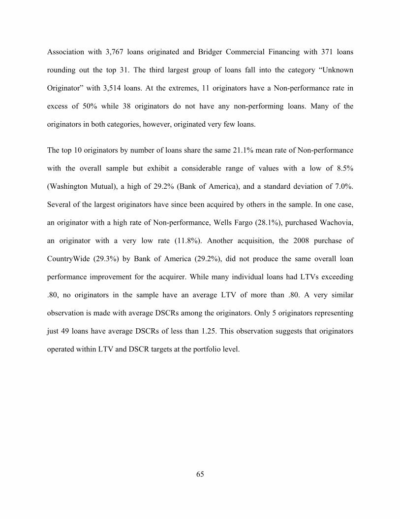
65

Association with 3,767 loans originated and Bridger Commercial Financing with 371 loans

rounding out the top 31. The third largest group of loans fall into the category “Unknown

Originator” with 3,514 loans. At the extremes, 11 originators have a Non-performance rate in

excess of 50% while 38 originators do not have any non-performing loans. Many of the

originators in both categories, however, originated very few loans.

The top 10 originators by number of loans share the same 21.1% mean rate of Non-performance

with the overall sample but exhibit a considerable range of values with a low of 8.5%

(Washington Mutual), a high of 29.2% (Bank of America), and a standard deviation of 7.0%.

Several of the largest originators have since been acquired by others in the sample. In one case,

an originator with a high rate of Non-performance, Wells Fargo (28.1%), purchased Wachovia,

an originator with a very low rate (11.8%). Another acquisition, the 2008 purchase of

CountryWide (29.3%) by Bank of America (29.2%), did not produce the same overall loan

performance improvement for the acquirer. While many individual loans had LTVs exceeding

.80, no originators in the sample have an average LTV of more than .80. A very similar

observation is made with average DSCRs among the originators. Only 5 originators representing

just 49 loans have average DSCRs of less than 1.25. This observation suggests that originators

operated within LTV and DSCR targets at the portfolio level.

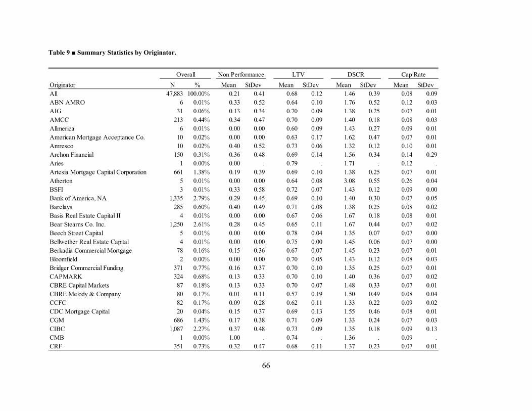
66

Table 9 ■ Summary Statistics by Originator.

Originator N % Mean StDev Mean StDev Mean StDev Mean StDevAll 47,883 100.00% 0.21 0.41 0.68 0.12 1.46 0.39 0.08 0.09ABN AMRO 6 0.01% 0.33 0.52 0.64 0.10 1.76 0.52 0.12 0.03AIG 31 0.06% 0.13 0.34 0.70 0.09 1.38 0.25 0.07 0.01AMCC 213 0.44% 0.34 0.47 0.70 0.09 1.40 0.18 0.08 0.03Allmerica 6 0.01% 0.00 0.00 0.60 0.09 1.43 0.27 0.09 0.01American Mortgage Acceptance Co. 10 0.02% 0.00 0.00 0.63 0.17 1.62 0.47 0.07 0.01Amresco 10 0.02% 0.40 0.52 0.73 0.06 1.32 0.12 0.10 0.01Archon Financial 150 0.31% 0.36 0.48 0.69 0.14 1.56 0.34 0.14 0.29Aries 1 0.00% 0.00 . 0.79 . 1.71 . 0.12 .Artesia Mortgage Capital Corporation 661 1.38% 0.19 0.39 0.69 0.10 1.38 0.25 0.07 0.01Atherton 5 0.01% 0.00 0.00 0.64 0.08 3.08 0.55 0.26 0.04BSFI 3 0.01% 0.33 0.58 0.72 0.07 1.43 0.12 0.09 0.00Bank of America, NA 1,335 2.79% 0.29 0.45 0.69 0.10 1.40 0.30 0.07 0.05Barclays 285 0.60% 0.40 0.49 0.71 0.08 1.38 0.25 0.08 0.02Basis Real Estate Capital II 4 0.01% 0.00 0.00 0.67 0.06 1.67 0.18 0.08 0.01Bear Stearns Co. Inc. 1,250 2.61% 0.28 0.45 0.65 0.11 1.67 0.44 0.07 0.02Beech Street Capital 5 0.01% 0.00 0.00 0.78 0.04 1.35 0.07 0.07 0.00Bellwether Real Estate Capital 4 0.01% 0.00 0.00 0.75 0.00 1.45 0.06 0.07 0.00Berkadia Commercial Mortgage 78 0.16% 0.15 0.36 0.67 0.07 1.45 0.23 0.07 0.01Bloomfield 2 0.00% 0.00 0.00 0.70 0.05 1.43 0.12 0.08 0.03Bridger Commercial Funding 371 0.77% 0.16 0.37 0.70 0.10 1.35 0.25 0.07 0.01CAPMARK 324 0.68% 0.13 0.33 0.70 0.10 1.40 0.36 0.07 0.02CBRE Capital Markets 87 0.18% 0.13 0.33 0.70 0.07 1.48 0.33 0.07 0.01CBRE Melody & Company 80 0.17% 0.01 0.11 0.57 0.19 1.50 0.49 0.08 0.04CCFC 82 0.17% 0.09 0.28 0.62 0.11 1.33 0.22 0.09 0.02CDC Mortgage Capital 20 0.04% 0.15 0.37 0.69 0.13 1.55 0.46 0.08 0.01CGM 686 1.43% 0.17 0.38 0.71 0.09 1.33 0.24 0.07 0.03CIBC 1,087 2.27% 0.37 0.48 0.73 0.09 1.35 0.18 0.09 0.13CMB 1 0.00% 1.00 . 0.74 . 1.36 . 0.09 .CRF 351 0.73% 0.32 0.47 0.68 0.11 1.37 0.23 0.07 0.01

Non Performance LTV DSCR Cap RateOverall

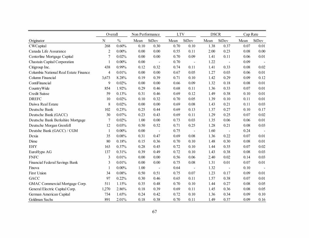
67

Originator N % Mean StDev Mean StDev Mean StDev Mean StDevCWCapital 268 0.60% 0.10 0.30 0.70 0.10 1.38 0.37 0.07 0.01Canada Life Assurance 2 0.00% 0.00 0.00 0.55 0.11 2.00 0.23 0.08 0.00Centerline Mortgage Capital 7 0.02% 0.00 0.00 0.70 0.09 1.41 0.11 0.06 0.01Chastain Capital Corporation 1 0.00% 0.00 - 0.70 - 1.22 - 0.09 -Citigroup Inc. 438 0.99% 0.12 0.32 0.74 0.11 1.41 0.33 0.08 0.02Columbia National Real Estate Finance 4 0.01% 0.00 0.00 0.67 0.05 1.27 0.03 0.06 0.01Column Financial 3,673 8.28% 0.19 0.39 0.71 0.10 1.42 0.29 0.09 0.12ContiFinancial 9 0.02% 0.00 0.00 0.66 0.09 1.32 0.18 0.08 0.01CountryWide 854 1.92% 0.29 0.46 0.68 0.11 1.36 0.33 0.07 0.01Credit Suisse 59 0.13% 0.31 0.46 0.69 0.12 1.49 0.38 0.10 0.01DREFC 10 0.02% 0.10 0.32 0.70 0.05 1.39 0.10 0.11 0.01Daiwa Real Estate 8 0.02% 0.00 0.00 0.69 0.08 1.43 0.21 0.11 0.03Deutsche Bank 102 0.23% 0.25 0.44 0.69 0.13 1.37 0.27 0.10 0.17Deutsche Bank (GACC) 30 0.07% 0.23 0.43 0.69 0.11 1.29 0.25 0.07 0.02Deutsche Bank Berkshire Mortgage 7 0.02% 1.00 0.00 0.73 0.03 1.35 0.06 0.06 0.01Deutsche Morgan Grenfell 12 0.03% 0.50 0.52 0.71 0.25 1.28 0.21 0.08 0.03Deutshe Bank (GACC) / CGM 1 0.00% 0.00 - 0.75 - 1.60 - 0.24 -Dexia 35 0.08% 0.31 0.47 0.69 0.08 1.36 0.22 0.07 0.01Dime 80 0.18% 0.15 0.36 0.70 0.10 1.48 0.30 0.08 0.01EHY 163 0.37% 0.28 0.45 0.72 0.10 1.44 0.35 0.07 0.02EuroHypo AG 137 0.31% 0.39 0.49 0.72 0.10 1.43 0.38 0.08 0.03FNFC 3 0.01% 0.00 0.00 0.56 0.06 2.40 0.02 0.14 0.03Financial Federal Savings Bank 3 0.01% 0.00 0.00 0.75 0.08 1.31 0.01 0.07 0.01Finova 1 0.00% 1.00 - 0.64 - 1.32 - 0.10 -First Union 34 0.08% 0.50 0.51 0.75 0.07 1.23 0.17 0.09 0.01GACC 97 0.22% 0.30 0.46 0.65 0.11 1.57 0.38 0.07 0.01GMAC Commercial Mortgage Corp. 511 1.15% 0.35 0.48 0.70 0.10 1.44 0.27 0.08 0.05General Electric Capital Corp. 1,270 2.86% 0.18 0.39 0.69 0.11 1.45 0.36 0.08 0.05German American Capital 734 1.65% 0.24 0.42 0.72 0.10 1.36 0.34 0.09 0.10Goldman Sachs 891 2.01% 0.18 0.38 0.70 0.11 1.49 0.37 0.09 0.16

Cap RateOverall Non Performance LTV DSCR

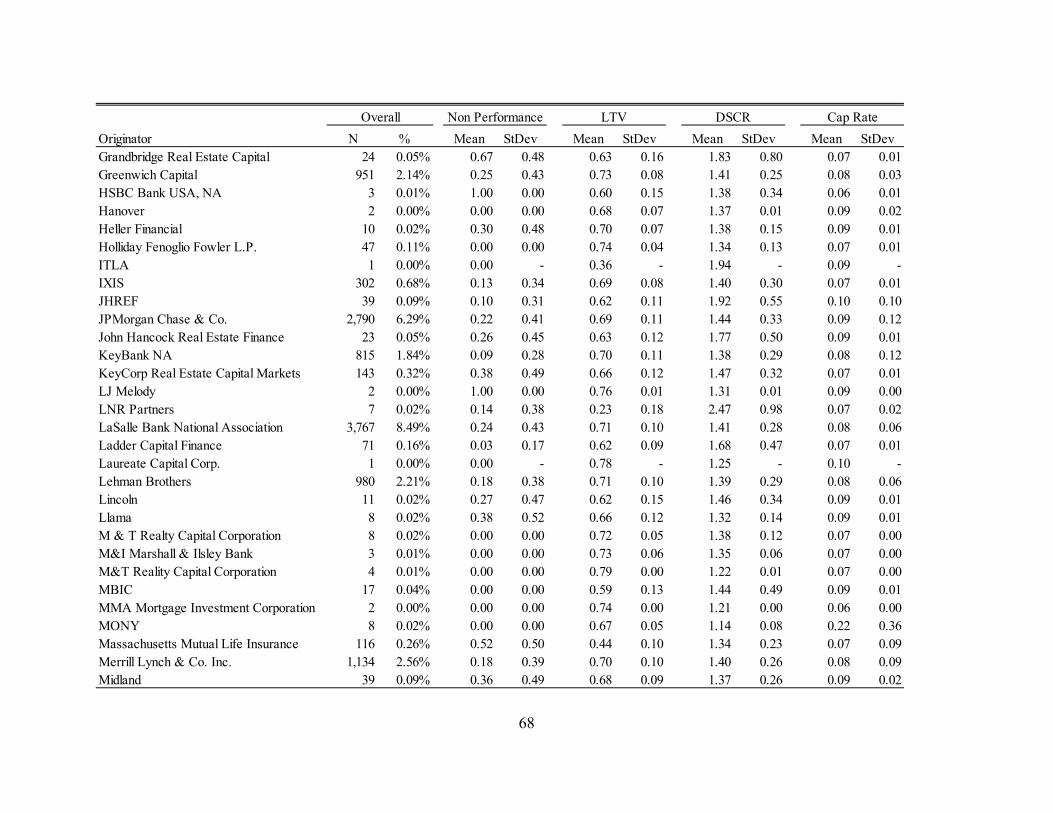
68

Originator N % Mean StDev Mean StDev Mean StDev Mean StDevGrandbridge Real Estate Capital 24 0.05% 0.67 0.48 0.63 0.16 1.83 0.80 0.07 0.01Greenwich Capital 951 2.14% 0.25 0.43 0.73 0.08 1.41 0.25 0.08 0.03HSBC Bank USA, NA 3 0.01% 1.00 0.00 0.60 0.15 1.38 0.34 0.06 0.01Hanover 2 0.00% 0.00 0.00 0.68 0.07 1.37 0.01 0.09 0.02Heller Financial 10 0.02% 0.30 0.48 0.70 0.07 1.38 0.15 0.09 0.01Holliday Fenoglio Fowler L.P. 47 0.11% 0.00 0.00 0.74 0.04 1.34 0.13 0.07 0.01ITLA 1 0.00% 0.00 - 0.36 - 1.94 - 0.09 -IXIS 302 0.68% 0.13 0.34 0.69 0.08 1.40 0.30 0.07 0.01JHREF 39 0.09% 0.10 0.31 0.62 0.11 1.92 0.55 0.10 0.10JPMorgan Chase & Co. 2,790 6.29% 0.22 0.41 0.69 0.11 1.44 0.33 0.09 0.12John Hancock Real Estate Finance 23 0.05% 0.26 0.45 0.63 0.12 1.77 0.50 0.09 0.01KeyBank NA 815 1.84% 0.09 0.28 0.70 0.11 1.38 0.29 0.08 0.12KeyCorp Real Estate Capital Markets 143 0.32% 0.38 0.49 0.66 0.12 1.47 0.32 0.07 0.01LJ Melody 2 0.00% 1.00 0.00 0.76 0.01 1.31 0.01 0.09 0.00LNR Partners 7 0.02% 0.14 0.38 0.23 0.18 2.47 0.98 0.07 0.02LaSalle Bank National Association 3,767 8.49% 0.24 0.43 0.71 0.10 1.41 0.28 0.08 0.06Ladder Capital Finance 71 0.16% 0.03 0.17 0.62 0.09 1.68 0.47 0.07 0.01Laureate Capital Corp. 1 0.00% 0.00 - 0.78 - 1.25 - 0.10 -Lehman Brothers 980 2.21% 0.18 0.38 0.71 0.10 1.39 0.29 0.08 0.06Lincoln 11 0.02% 0.27 0.47 0.62 0.15 1.46 0.34 0.09 0.01Llama 8 0.02% 0.38 0.52 0.66 0.12 1.32 0.14 0.09 0.01M & T Realty Capital Corporation 8 0.02% 0.00 0.00 0.72 0.05 1.38 0.12 0.07 0.00M&I Marshall & Ilsley Bank 3 0.01% 0.00 0.00 0.73 0.06 1.35 0.06 0.07 0.00M&T Reality Capital Corporation 4 0.01% 0.00 0.00 0.79 0.00 1.22 0.01 0.07 0.00MBIC 17 0.04% 0.00 0.00 0.59 0.13 1.44 0.49 0.09 0.01MMA Mortgage Investment Corporation 2 0.00% 0.00 0.00 0.74 0.00 1.21 0.00 0.06 0.00MONY 8 0.02% 0.00 0.00 0.67 0.05 1.14 0.08 0.22 0.36Massachusetts Mutual Life Insurance 116 0.26% 0.52 0.50 0.44 0.10 1.34 0.23 0.07 0.09Merrill Lynch & Co. Inc. 1,134 2.56% 0.18 0.39 0.70 0.10 1.40 0.26 0.08 0.09Midland 39 0.09% 0.36 0.49 0.68 0.09 1.37 0.26 0.09 0.02

Overall Non Performance LTV DSCR Cap Rate

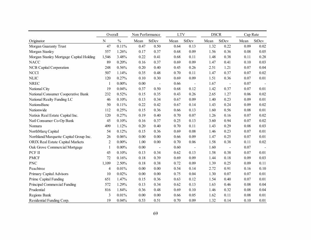
69

Originator N % Mean StDev Mean StDev Mean StDev Mean StDevMorgan Guaranty Trust 47 0.11% 0.47 0.50 0.64 0.13 1.32 0.22 0.09 0.02Morgan Stanley 557 1.26% 0.17 0.37 0.68 0.09 1.56 0.36 0.08 0.05Morgan Stanley Mortgage Capital Holding 1,546 3.48% 0.22 0.41 0.68 0.11 1.48 0.38 0.11 0.28NACC 89 0.20% 0.16 0.37 0.69 0.09 1.47 0.41 0.10 0.03NCB Capital Corporation 248 0.56% 0.20 0.40 0.45 0.26 2.51 1.21 0.07 0.04NCCI 507 1.14% 0.35 0.48 0.70 0.11 1.47 0.37 0.07 0.02NLIC 120 0.27% 0.10 0.30 0.69 0.09 1.51 0.36 0.07 0.01NREC 1 0.00% 0.00 - 0.66 - 1.67 - 0.07 -National City 19 0.04% 0.37 0.50 0.68 0.12 1.42 0.37 0.07 0.01National Consumer Cooperative Bank 232 0.52% 0.15 0.35 0.43 0.26 2.65 1.27 0.06 0.02National Realty Funding LC 46 0.10% 0.13 0.34 0.67 0.09 1.40 0.23 0.09 0.01NationsBanc 50 0.11% 0.22 0.42 0.67 0.14 1.43 0.24 0.09 0.02Nationwide 112 0.25% 0.15 0.36 0.66 0.13 1.60 0.56 0.08 0.01Natixis Real Estate Capital Inc. 120 0.27% 0.19 0.40 0.70 0.07 1.26 0.16 0.07 0.02Natl Consumer Co-Op Bank 45 0.10% 0.16 0.37 0.25 0.13 3.60 0.94 0.07 0.02Nomura 499 1.12% 0.20 0.40 0.70 0.11 1.43 0.29 0.08 0.03NorthMarq Capital 54 0.12% 0.15 0.36 0.69 0.08 1.46 0.23 0.07 0.01Northland/Marquette Capital Group Inc. 26 0.06% 0.00 0.00 0.66 0.09 1.47 0.25 0.07 0.01ORIX Real Estate Capital Markets 2 0.00% 1.00 0.00 0.70 0.06 1.58 0.38 0.11 0.02Oak Grove Commercial Mortgage 1 0.00% 0.00 - 0.60 - 1.60 - 0.07 -PCF II 45 0.10% 0.13 0.34 0.62 0.13 1.58 0.38 0.07 0.01PMCF 72 0.16% 0.18 0.39 0.69 0.09 1.44 0.18 0.09 0.03PNC 1,109 2.50% 0.18 0.38 0.72 0.09 1.39 0.25 0.09 0.11Peachtree 4 0.01% 0.00 0.00 0.54 0.14 2.72 0.91 0.16 0.10Primary Capital Advisors 10 0.02% 0.00 0.00 0.75 0.04 1.30 0.07 0.07 0.01Prime Capital Funding 651 1.47% 0.15 0.36 0.63 0.12 1.54 0.40 0.07 0.01Principal Commercial Funding 572 1.29% 0.13 0.34 0.62 0.13 1.63 0.46 0.08 0.04Prudential 816 1.84% 0.36 0.48 0.69 0.10 1.46 0.32 0.08 0.04Regions Bank 3 0.01% 0.00 0.00 0.66 0.05 1.62 0.11 0.08 0.01Residential Funding Corp. 19 0.04% 0.53 0.51 0.70 0.09 1.32 0.14 0.10 0.01

Non Performance LTV DSCR Cap RateOverall

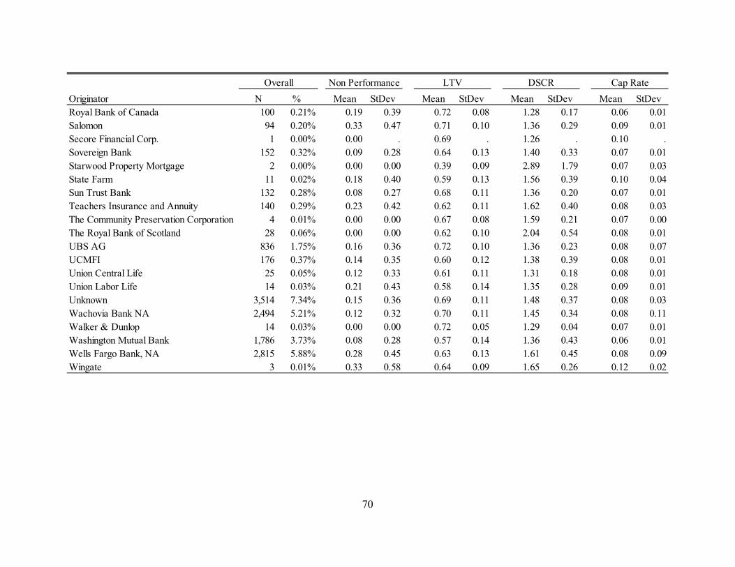
70

Originator N % Mean StDev Mean StDev Mean StDev Mean StDevRoyal Bank of Canada 100 0.21% 0.19 0.39 0.72 0.08 1.28 0.17 0.06 0.01Salomon 94 0.20% 0.33 0.47 0.71 0.10 1.36 0.29 0.09 0.01Secore Financial Corp. 1 0.00% 0.00 . 0.69 . 1.26 . 0.10 .Sovereign Bank 152 0.32% 0.09 0.28 0.64 0.13 1.40 0.33 0.07 0.01Starwood Property Mortgage 2 0.00% 0.00 0.00 0.39 0.09 2.89 1.79 0.07 0.03State Farm 11 0.02% 0.18 0.40 0.59 0.13 1.56 0.39 0.10 0.04Sun Trust Bank 132 0.28% 0.08 0.27 0.68 0.11 1.36 0.20 0.07 0.01Teachers Insurance and Annuity 140 0.29% 0.23 0.42 0.62 0.11 1.62 0.40 0.08 0.03The Community Preservation Corporation 4 0.01% 0.00 0.00 0.67 0.08 1.59 0.21 0.07 0.00The Royal Bank of Scotland 28 0.06% 0.00 0.00 0.62 0.10 2.04 0.54 0.08 0.01UBS AG 836 1.75% 0.16 0.36 0.72 0.10 1.36 0.23 0.08 0.07UCMFI 176 0.37% 0.14 0.35 0.60 0.12 1.38 0.39 0.08 0.01Union Central Life 25 0.05% 0.12 0.33 0.61 0.11 1.31 0.18 0.08 0.01Union Labor Life 14 0.03% 0.21 0.43 0.58 0.14 1.35 0.28 0.09 0.01Unknown 3,514 7.34% 0.15 0.36 0.69 0.11 1.48 0.37 0.08 0.03Wachovia Bank NA 2,494 5.21% 0.12 0.32 0.70 0.11 1.45 0.34 0.08 0.11Walker & Dunlop 14 0.03% 0.00 0.00 0.72 0.05 1.29 0.04 0.07 0.01Washington Mutual Bank 1,786 3.73% 0.08 0.28 0.57 0.14 1.36 0.43 0.06 0.01Wells Fargo Bank, NA 2,815 5.88% 0.28 0.45 0.63 0.13 1.61 0.45 0.08 0.09Wingate 3 0.01% 0.33 0.58 0.64 0.09 1.65 0.26 0.12 0.02

Cap RateOverall Non Performance LTV DSCR

71

Empirical Results

Cap Rate Spread: Full Sample

The first model estimates the relationship between Cap Rate Spread, its covariates, and CMBS

loan Non-performance. The parameters are estimated using two versions of the model with one

including LTV and another with DSCR. The results are presented in Table 10. The LTV

coefficient in the LTV model is positive as expected, estimated to be 1.05 and significant at the

1% level. Due to the shape of the cumulative normal distribution, the effects of the coefficients

are dependent upon the starting point along the curve.

As illustrated by Pampel (2000), the probit coefficients are difficult to interpret in their “raw”

form but may be transformed into more manageable terms. The LTV coefficient of 1.05

represents the change in the probit / z-score for a 1 unit change in LTV. This effect equates to

different changes in probability depending upon the starting point due to the shape of the

cumulative normal distribution. The effect will be greatest where the probability of the

dependent variable is closest to .5 and diminish as probability Non-performance moves in either

direction.

The mean level of Non-performance in the CMBS loan is .21 meaning that 21% of loans have a

status of Non-performance. This value of .21 translates to a z-score of -.81 with a probability

density of .29. Multiplying this coefficient for LTV of 1.05 by the probability density for Non-

performance at its mean (.29) the result is .30 which represents the change in probability for a 1

unit change in LTV. This relationship suggests that an increase in LTV of .05, from .70 to .75

72

would increase the probability of Non-performance by 1.5% (.05 x .30 = .015). The same

approach may be used for the interpretation of the other probit coefficients in this dissertation.

The coefficient for LnSIZE, the natural log of loan size, in the estimation of Equation (12) for the

LTV and DSCR models and all subsequent estimations is positive and significant, suggesting

that as loans increase in size, the probability of Non-performance also increases. The size and

significance of the coefficient for loan size (LnSIZE) in the LTV model of Table 10 is .04 and

less than 1% respectively.

The coefficient for CMBS origination volume (DEALS) is significant and negative, suggesting

that as origination volume increases, the risk of Non-performance decreases. This result seems to

contradict the conventional wisdom that increased deal volume enables lower quality loans to

slip through. An alternative explanation for this finding may be attributed to increased

experience and competence of underwriters who have recently completed more transactions or

underwriting teams who have, in the wake recent origination volume, increased their staffing

levels or implemented standards designed to deal with the surge in origination volume. This

alternative hypothesis suggests the possibility of a negative relation between origination volume

and Non-performance.

The CPNSPRD (Coupon Spread) coefficients in both LTV and DSCR models of Table 10 are

significant and positive with increased gaps between the current 10-Year Treasury note and the

coupon rate on the loan associated with higher levels of Non-performance. A higher Coupon

Spread proxies the pricing of riskier loans at origination and the evidence of increased risk for

Non-performance justifies the pricing.

73

The final variable in the estimation of the LTV and DSCR models reported in Table 10 is

CAPSPRD (Cap Rate Spread). The parameter estimates for CAPSPRD are negative as expected

in both models but only significant in the LTV model. A third model, not reported in Table 10,

includes both LTV and DSCR produces results similar to those of the LTV only model, the

coefficient for DSCR insignificant. Results from Table 10 provide limited support for the

hypothesis that the Cap Rate Spread is related to Non-performance among all CMBS loan types.

The results from the LTV and DSCR models are inconsistent since Cap Rate Spread is not

significant in the DSCR model.

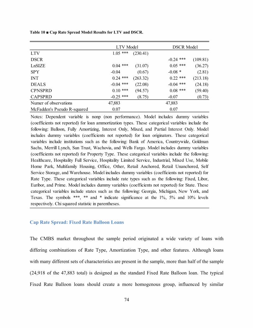
74

Table 10 ■ Cap Rate Spread Model Results for LTV and DSCR.

Cap Rate Spread: Fixed Rate Balloon Loans

The CMBS market throughout the sample period originated a wide variety of loans with

differing combinations of Rate Type, Amortization Type, and other features. Although loans

with many different sets of characteristics are present in the sample, more than half of the sample

(24,918 of the 47,883 total) is designed as the standard Fixed Rate Balloon loan. The typical

Fixed Rate Balloon loans should create a more homogenous group, influenced by similar

LTV 1.05 *** (230.41)DSCR -0.24 *** (109.81)LnSIZE 0.04 *** (31.07) 0.05 *** (36.27)SPY -0.04 (0.67) -0.08 * (2.81)INT 0.24 *** (263.32) 0.22 *** (213.18)DEALS -0.04 *** (22.08) -0.04 *** (24.18)CPNSPRD 0.10 *** (94.57) 0.08 *** (59.40)CAPSPRD -0.25 *** (8.75) -0.07 (0.73)Numer of observations 47,883 47,883 McFadden's Pseudo R-squared 0.07 0.07

Notes: Dependent variable is nonp (non performance). Model includes dummy variables(coefficients not reported) for loan ammortization types. These categorical variables include thefollowing: Balloon, Fully Amortizing, Interest Only, Mixed, and Partial Interest Only. Modelincludes dummy variables (coefficients not reported) for loan originators. These categoricalvariables include institutions such as the following: Bank of America, Countrywide, GoldmanSachs, Merrill Lynch, Sun Trust, Wachovia, and Wells Fargo. Model includes dummy variables(coefficients not reported) for Property Type. These categorical variables include the following:Healthcare, Hospitality Full Service, Hospitality Limited Service, Industrial, Mixed Use, MobileHome Park, Multifamily Housing, Office, Other, Retail Anchored, Retail Unanchored, SelfService Storage, and Warehouse. Model includes dummy variables (coefficients not reported) forRate Type. These categorical variables include rate types such as the following: Fixed, Libor,Euribor, and Prime. Model includes dummy variables (coefficients not reported) for State. Thesecategorical variables include states such as the following: Georgia, Michigan, New York, andTexas. The symbols ***, ** and * indicate significance at the 1%, 5% and 10% levelsrespectively. Chi squared statistic in parentheses.

LTV Model DSCR Model

75

unmeasured risk and underwriting variables. To investigate the Cap Rate Spread relationship

further, the sample is split into two groups: Fixed Rate Balloon loans, and all other loans.

Estimation with LTV: Fixed Rate Balloon Loans Only

The Fixed Rate Balloon loan subset includes only those loans with both characteristics: a Rate

Type of Fixed and an Amortization Type of Balloon. This is the most common type of loan

packaged and sold to the CMBS market. In addition to all other Rate and Amortization Types,

the subset of other loans includes Fixed Rate loans and Balloon loans paired with non-Balloon

Amortization Types and non-Fixed Rate Types respectively. Table 11 presents the results for the

two sample subsets, with the Fixed Rate Balloon loans in Panel A and all other loans in Panel B.

The results for Fixed Rate Balloon loans support a significant role for Cap Rate Spread in both

the models for LTV and DSCR. In the Panel A of Table 11 for the LTV model, the estimated

coefficients for LTV, loan size, interest rates, recent origination volume, Coupon Spread, and

Cap Rate Spread are consistent with the results in both significance and direction to those in

Table 10 for the full sample. With the Fixed Rate Balloon subset, the effect size for Cap Rate

Spread in the LTV model is nearly double that of the full sample (-.25 compared to -.48),

suggesting that the risk of Non-performance attributable to the Cap Rate Spread is considerably

greater for Fixed rate Balloon loans.

Estimation with DSCR: Fixed Rate Balloon Loans Only

The DSCR model in Panel A of Table 11 also presents results that are largely consistent with

those of the full sample in Table 10, with the exception of the finding for the Cap Rate Spread.

For the standard Fixed Rate Balloon loans, CAPSPRD (Cap Rate Spread) has a negative and

76

significant impact on the risk of Non-performance in the DSCR model. This finding suggests

that the Cap Rate Spread is a predictor of Non-performance for Fixed Rate Balloon loans, and

that estimations considering alternative less-standard mortgage structures veil this relationship.

The Panel A model fit statistics reported by the McFadden’s pseudo R-square are the same

between Table 10 and Table 11 at .07 for all specifications.

All Other Amortization Types

Panel B of Table 11 reports the model results for the subset of the database with all other types

of loans that do not combine Fixed Rate and Balloon Amortization. This collection of different

types of loans shares some of the same parameter estimates with the full sample reported in

Table 10 with a few notable exceptions. A relationship between Non-performance and recent

stock market performance is not detected in the LTV model for the full sample and is just barely

significant by standard criteria in the DSCR model of Table 10. In contrast, a Non-performance

relationship with the stock market is significant at the 5% and 1% level in the LTV and DSCR

models, respectively, in Panel B. The relationship between recent stock market returns and Non-

performance is negative, suggesting that as the level of recent stock market returns rises, the

level of CMBS loan Non-performance falls among these other types of loans.

Results describing the stock market relationship reported in Table 11 Panel B provide an

interesting possible direction for future research. The results may be due to stock market

momentum and/or sentiment among underwriters whereby loans originated following periods of

higher stock market returns may only be sold to debt investors who are more discriminating and

thus requiring more stringent underwriting and higher quality loans. Following periods of lower

stock market returns, more investors may flock to the apparent security of bonds, debt and MBS

77

causing a demand driven push to originate marginal, lower quality loans approved by less

stringent underwriters.

In contrast to Panel A, the Cap Rate Spread coefficient of the DSCR model in Panel B is

positive. For this group of non-Fixed Rate Balloon loans, Non-performance rises as the Cap Rate

Spread increases. This result suggests that among this subset of loans, the absolute level of Cap

Rate is binding in the relationship with Non-performance. This finding is consistent with the

conventional wisdom associating high Cap Rates with high risk real estate but is at odds with the

theory that a low Cap Rate Spread increases the probability of Non-performance.

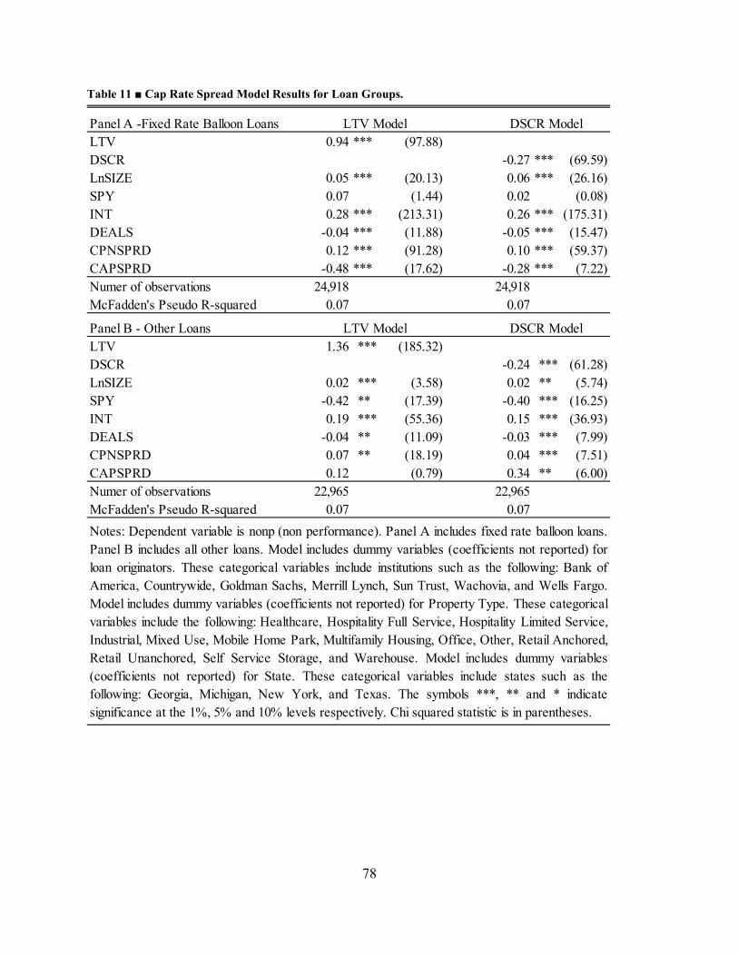
78

Table 11 ■ Cap Rate Spread Model Results for Loan Groups.

Panel A -Fixed Rate Balloon LoansLTV 0.94 *** (97.88)DSCR -0.27 *** (69.59)LnSIZE 0.05 *** (20.13) 0.06 *** (26.16)SPY 0.07 (1.44) 0.02 (0.08)INT 0.28 *** (213.31) 0.26 *** (175.31)DEALS -0.04 *** (11.88) -0.05 *** (15.47)CPNSPRD 0.12 *** (91.28) 0.10 *** (59.37)CAPSPRD -0.48 *** (17.62) -0.28 *** (7.22)Numer of observations 24,918 24,918 McFadden's Pseudo R-squared 0.07 0.07

Panel B - Other LoansLTV 1.36 *** (185.32)DSCR -0.24 *** (61.28)LnSIZE 0.02 *** (3.58) 0.02 ** (5.74)SPY -0.42 ** (17.39) -0.40 *** (16.25)INT 0.19 *** (55.36) 0.15 *** (36.93)DEALS -0.04 ** (11.09) -0.03 *** (7.99)CPNSPRD 0.07 ** (18.19) 0.04 *** (7.51)CAPSPRD 0.12 (0.79) 0.34 ** (6.00)Numer of observations 22,965 22,965 McFadden's Pseudo R-squared 0.07 0.07

LTV Model DSCR Model

Notes: Dependent variable is nonp (non performance). Panel A includes fixed rate balloon loans.Panel B includes all other loans. Model includes dummy variables (coefficients not reported) forloan originators. These categorical variables include institutions such as the following: Bank ofAmerica, Countrywide, Goldman Sachs, Merrill Lynch, Sun Trust, Wachovia, and Wells Fargo.Model includes dummy variables (coefficients not reported) for Property Type. These categoricalvariables include the following: Healthcare, Hospitality Full Service, Hospitality Limited Service,Industrial, Mixed Use, Mobile Home Park, Multifamily Housing, Office, Other, Retail Anchored,Retail Unanchored, Self Service Storage, and Warehouse. Model includes dummy variables(coefficients not reported) for State. These categorical variables include states such as thefollowing: Georgia, Michigan, New York, and Texas. The symbols ***, ** and * indicatesignificance at the 1%, 5% and 10% levels respectively. Chi squared statistic is in parentheses.

LTV Model DSCR Model

79

Cap Rate Spread and Non-performance: Conservative Loans

For Cap Rate Spread to aid in evaluating commercial mortgage risk, it must provide information

beyond the analysis techniques already in use by industry experts and academic researchers.

Conservative underwriting standards relying upon LTV and DSCR will still permit the

origination of some subsequently non-performing loans. Starting with the sample used in Panel

A of Table 11, fixed rate balloon loans, the sample is filtered further, selecting only those loans

which would meet typical underwriter requirements in both areas, LTV and DSCR. Using only

loans which would pass a conservative set of LTV and DSCR criteria, .80 and 1.25 respectively,

the Cap Rate Spread coefficient now provides an indication of the additional information

provided by this measure even among loans normally considered very conservative.

Although the sample includes only loans with LTV less than .8 and DSCR greater than 1.25, the

specifications estimated retain these variables as these variables likely continue to be related to

Non-performance even in these “safe” ranges. Table 12 presents the results of the model with

this sample of presumably safe loans and indicates that Cap Rate Spread is a significantly related

to Non-performance in the direction expected. The effect size of Cap Rate Spread approaches

LTV and even exceeds that of DSCR in this restricted set of loans as expected since these loans

have already been filtered to eliminate those with the most extreme LTV and DSCR values.

The effects are important in this group because this is a group of loans which would escape even

the conservative underwriter’s scrutiny insofar as the LTV and DSCR measures are concerned.

As with the full sample of fixed rate balloon loans, as the Cap Rate Spread falls, the incidence of

Non-performance rises. This result is consistent in scale, direction, and significance to those of

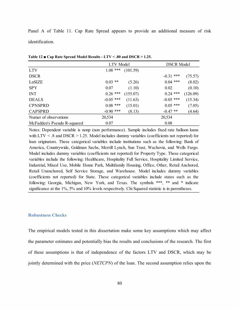
80

Panel A of Table 11. Cap Rate Spread appears to provide an additional measure of risk

identification.

Table 12 ■ Cap Rate Spread Model Results - LTV < .80 and DSCR > 1.25.

Robustness Checks

The empirical models tested in this dissertation make some key assumptions which may affect

the parameter estimates and potentially bias the results and conclusions of the research. The first

of these assumptions is that of independence of the factors LTV and DSCR, which may be

jointly determined with the price (NETCPN) of the loan. The second assumption relies upon the

LTV 1.08 *** (101.59)DSCR -0.31 *** (75.57)LnSIZE 0.03 ** (5.26) 0.04 *** (8.02)SPY 0.07 (1.10) 0.02 (0.10)INT 0.26 *** (155.07) 0.24 *** (126.09)DEALS -0.05 *** (11.63) -0.05 *** (15.34)CPNSPRD 0.08 *** (15.01) 0.05 *** (7.05)CAPSPRD -0.90 *** (8.13) -0.47 ** (4.64)Numer of observations 20,534 20,534 McFadden's Pseudo R-squared 0.07 0.08

Notes: Dependent variable is nonp (non performance). Sample includes fixed rate balloon loanswith LTV < .8 and DSCR > 1.25. Model includes dummy variables (coefficients not reported) forloan originators. These categorical variables include institutions such as the following: Bank ofAmerica, Countrywide, Goldman Sachs, Merrill Lynch, Sun Trust, Wachovia, and Wells Fargo.Model includes dummy variables (coefficients not reported) for Property Type. These categoricalvariables include the following: Healthcare, Hospitality Full Service, Hospitality Limited Service,Industrial, Mixed Use, Mobile Home Park, Multifamily Housing, Office, Other, Retail Anchored,Retail Unanchored, Self Service Storage, and Warehouse. Model includes dummy variables(coefficients not reported) for State. These categorical variables include states such as thefollowing: Georgia, Michigan, New York, and Texas. The symbols ***, ** and * indicatesignificance at the 1%, 5% and 10% levels respectively. Chi Squared statistic is in parentheses.

LTV Model DSCR Model

81

cumulative standard normal distribution to accurately describe the relationship between the

probability of Non-performance and the independent variables in the models used to test the

research hypotheses. Each of these assumptions is challenged in a series of robustness checks,

with results reported in the section below.

Interest Rate Endogeneity

The pricing of commercial mortgages involves a myriad of factors and risk mitigation tools that

range from the interest rate and ratio requirements of the loan to yield-maintenance provisions

and contractual covenants. Among the group of numerical considerations, factors such as the

coupon rate, LTV, and DSCR requirements are likely intertwined in the underwriting decision-

making process. A loan with a higher LTV or lower DSCR may be approved with a higher

interest rate. Conversely, loans with very conservative ratio results may be underwritten with

lower interest rates. This potential endogeneity may introduce bias in estimates of the Cap Rate

Spread in specifications including both the loan coupon rate (or calculated values relying upon it)

and the LTV or DSCR ratios.

The LTV should be related to Coupon Rate through the recognition among underwriters that a

loan with a higher LTV is riskier. As such, it is reasonable to expect that higher LTVs are

associated with higher rates. Borrowers requiring very high loan amounts relative to the value of

the collateral are sure to receive offers from lenders that feature commensurately higher interest

rates. Similarly, borrowers with a target or required level of interest will likely face limits on the

amount they may be borrowed and thus constrain the LTV possible for the deal.

82

The relation between loan interest rates and DSCR is even clearer, as higher interest rates

directly affect the DSCR by increasing the payment required for a given loan amount. A complex

interplay between the Coupon Rate, DSCR, and loan amount may also surface, as attempts by

lenders to compensate for the risk of a low DSCR tend to exacerbate the very ratio of concern.

As a risk-averse lender raises the rates to a low-DSCR borrower, the DSCR is even further

reduced when this outcome is not offset by a lower loan amount. Although the focus of this

analysis is constrained to LTV, DSCR and the Coupon Rate, many other factors may also be

adjusted as underwriters price commercial loans. Factors such as yield-maintenance protections,

rate type, amortization period, and other contractual provisions may also be modified by lenders

to counteract the risks of high LTV or low DSCR when their ability to adjust the loan interest

rate is limited.

To reduce the possibility of bias related to the endogeneity of loan rate and the ratios, a two-stage

model is specified wherein the loan coupon rate is predicted as a function of the ratios LTV and

DSCR, the 10-Year Treasury rate, indicator variables used in the other specifications, and a set

of indicator variables not included in the second-stage of the specification. In order to identify

the first-stage of the two-stage model, indicator variables for the time period are included in the

first-stage of the model. The results of the first-stage of the model are presented in Table 13. All

primary covariates are significant in the first-stage model including DSCR, LTV, and the 10-

Year Treasury rate. Of the 72 quarterly indicator variables, 53 (73.6%) are significant at the 1%

level, 2 (2.8%) are significant at the 5% level, 4 (5.6%) are significant at the 10% level, and the

remaining 13 (18.1%) fail to satisfy a significance test at any of the customary levels. The

second-stage of the specification predicts Non-performance as a function of Cap Rate Spread and

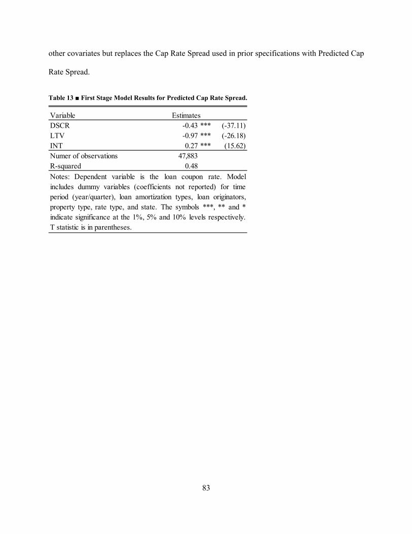
83

other covariates but replaces the Cap Rate Spread used in prior specifications with Predicted Cap

Rate Spread.

Table 13 ■ First Stage Model Results for Predicted Cap Rate Spread.

Variable EstimatesDSCR -0.43 *** (-37.11)LTV -0.97 *** (-26.18)INT 0.27 *** (15.62)Numer of observations 47,883 R-squared 0.48

Notes: Dependent variable is the loan coupon rate. Modelincludes dummy variables (coefficients not reported) for timeperiod (year/quarter), loan amortization types, loan originators,property type, rate type, and state. The symbols ***, ** and *indicate significance at the 1%, 5% and 10% levels respectively.T statistic is in parentheses.

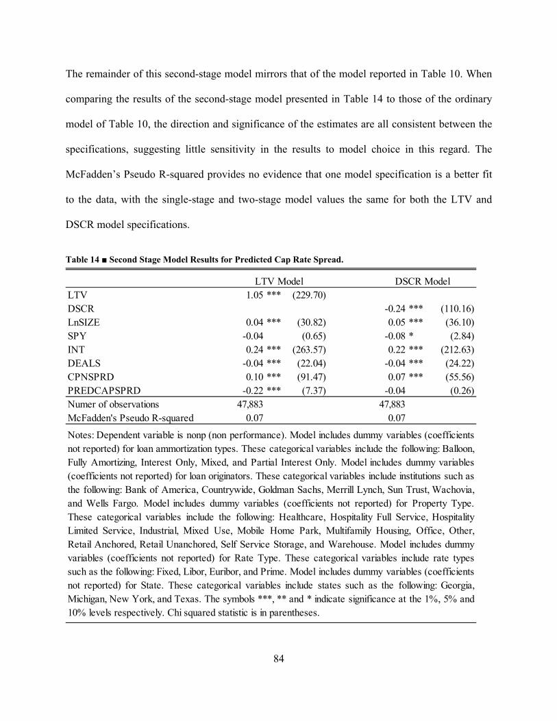
84

The remainder of this second-stage model mirrors that of the model reported in Table 10. When

comparing the results of the second-stage model presented in Table 14 to those of the ordinary

model of Table 10, the direction and significance of the estimates are all consistent between the

specifications, suggesting little sensitivity in the results to model choice in this regard. The

McFadden’s Pseudo R-squared provides no evidence that one model specification is a better fit

to the data, with the single-stage and two-stage model values the same for both the LTV and

DSCR model specifications.

Table 14 ■ Second Stage Model Results for Predicted Cap Rate Spread.

LTV 1.05 *** (229.70)DSCR -0.24 *** (110.16)LnSIZE 0.04 *** (30.82) 0.05 *** (36.10)SPY -0.04 (0.65) -0.08 * (2.84)INT 0.24 *** (263.57) 0.22 *** (212.63)DEALS -0.04 *** (22.04) -0.04 *** (24.22)CPNSPRD 0.10 *** (91.47) 0.07 *** (55.56)PREDCAPSPRD -0.22 *** (7.37) -0.04 (0.26)Numer of observations 47,883 47,883 McFadden's Pseudo R-squared 0.07 0.07

Notes: Dependent variable is nonp (non performance). Model includes dummy variables (coefficientsnot reported) for loan ammortization types. These categorical variables include the following: Balloon,Fully Amortizing, Interest Only, Mixed, and Partial Interest Only. Model includes dummy variables(coefficients not reported) for loan originators. These categorical variables include institutions such asthe following: Bank of America, Countrywide, Goldman Sachs, Merrill Lynch, Sun Trust, Wachovia,and Wells Fargo. Model includes dummy variables (coefficients not reported) for Property Type.These categorical variables include the following: Healthcare, Hospitality Full Service, HospitalityLimited Service, Industrial, Mixed Use, Mobile Home Park, Multifamily Housing, Office, Other,Retail Anchored, Retail Unanchored, Self Service Storage, and Warehouse. Model includes dummyvariables (coefficients not reported) for Rate Type. These categorical variables include rate typessuch as the following: Fixed, Libor, Euribor, and Prime. Model includes dummy variables (coefficientsnot reported) for State. These categorical variables include states such as the following: Georgia,Michigan, New York, and Texas. The symbols ***, ** and * indicate significance at the 1%, 5% and10% levels respectively. Chi squared statistic is in parentheses.

LTV Model DSCR Model

85

To test for model sensitivity among the Fixed Rate Balloon Loan subsample, the two-stage

approach is also applied to the model approach previously reported in Table 11. As with the prior

two-stage specification, the Coupon Rate for the individual loans is predicted in the first-stage.

The predicted loan Coupon Rate (PREDNETCPN) is then used in the construction of the Cap

Rate Spread (PREDCAPSPRD) entered into the second-stage equation. The results of the

second-stage model for specification testing loan groups are presented in Table 15. The estimates

for the group of Fixed Rate Balloon loans are presented in Panel A and are consistent with the

results in Panel A of Table 11. The estimates for other loans are presented in Panel B and are

also consistent with the results in Panel B of Table 11. The results presented in Table 15 provide

additional support with results for Cap Rate Spread that are insensitive to potential endogeneity

between loan rates and the LTV / DSCR ratios.

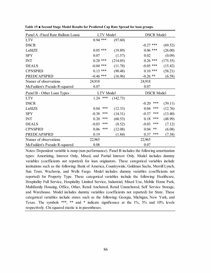
86

Table 15 ■ Second Stage Model Results for Predicted Cap Rate Spread for loan groups.

Panel A -Fixed Rate Balloon LoansLTV 0.94 *** (97.60)DSCR -0.27 *** (69.52)LnSIZE 0.05 *** (19.89) 0.06 *** (26.00)SPY 0.07 (1.57) 0.02 (0.09)INT 0.28 *** (214.05) 0.26 *** (175.55)DEALS -0.04 *** (11.78) -0.05 *** (15.42)CPNSPRD 0.13 *** (90.48) 0.10 *** (58.21)PREDCAPSPRD -0.46 *** (16.96) -0.26 ** (6.58)Numer of observations 24,918 24,918 McFadden's Pseudo R-squared 0.07 0.07

Panel B - Other Loan TypesLTV 1.24 *** (142.73)DSCR -0.20 *** (39.11)LnSIZE 0.04 *** (12.33) 0.04 *** (12.76)SPY -0.38 *** (14.31) -0.37 *** (13.40)INT 0.20 *** (60.53) 0.18 *** (48.99)DEALS -0.03 *** (8.52) -0.03 *** (7.12)CPNSPRD 0.06 *** (12.08) 0.04 ** (6.08)PREDCAPSPRD 0.19 (1.84) 0.37 *** (7.38)Numer of observations 22,965 22,965 McFadden's Pseudo R-squared 0.08 0.07

LTV Model DSCR Model

Notes: Dependent variable is nonp (non performance). Panel B includes the following amortization types: Amortizing, Interest Only, Mixed, and Partial Interest Only. Model includes dummyvariables (coefficients not reported) for loan originators. These categorical variables includeinstitutions such as the following: Bank of America, Countrywide, Goldman Sachs, Merrill Lynch,Sun Trust, Wachovia, and Wells Fargo. Model includes dummy variables (coefficients notreported) for Property Type. These categorical variables include the following: Healthcare,Hospitality Full Service, Hospitality Limited Service, Industrial, Mixed Use, Mobile Home Park,Multifamily Housing, Office, Other, Retail Anchored, Retail Unanchored, Self Service Storage,and Warehouse. Model includes dummy variables (coefficients not reported) for State. Thesecategorical variables include states such as the following: Georgia, Michigan, New York, andTexas. The symbols ***, ** and * indicate significance at the 1%, 5% and 10% levelsrespectively. Chi squared stastic is in parentheses.

LTV Model DSCR Model

87

Normal and Logistic Distributions

The empirical results presented thus far using probit models may be sensitive to the distribution

assumption of this approach. The probit technique assumes that the relationship takes the form of

the cumulative distribution function of the normal distribution. If this assumption is false,

estimates from probit models may suffer from bias and lead to erroneous conclusions. To test for

sensitivity to the distribution function choice, an alternative specification is used for two of the

empirical models. The Cap Rate Spread models with results presented in Table 10 for both LTV

and DSCR are performed again using a logit (logistic regression) model instead of a probit

model.

The results of this process are presented in Table 16. The direction and significance of the

estimates resulting from the logistic model are nearly identical to those resulting from the probit

model in Table 10. The direction, significance, and model fit, as indicated by the McFadden’s

pseudo R-squared, suggest little difference between the probit and logit models with this sample

and primary research question.

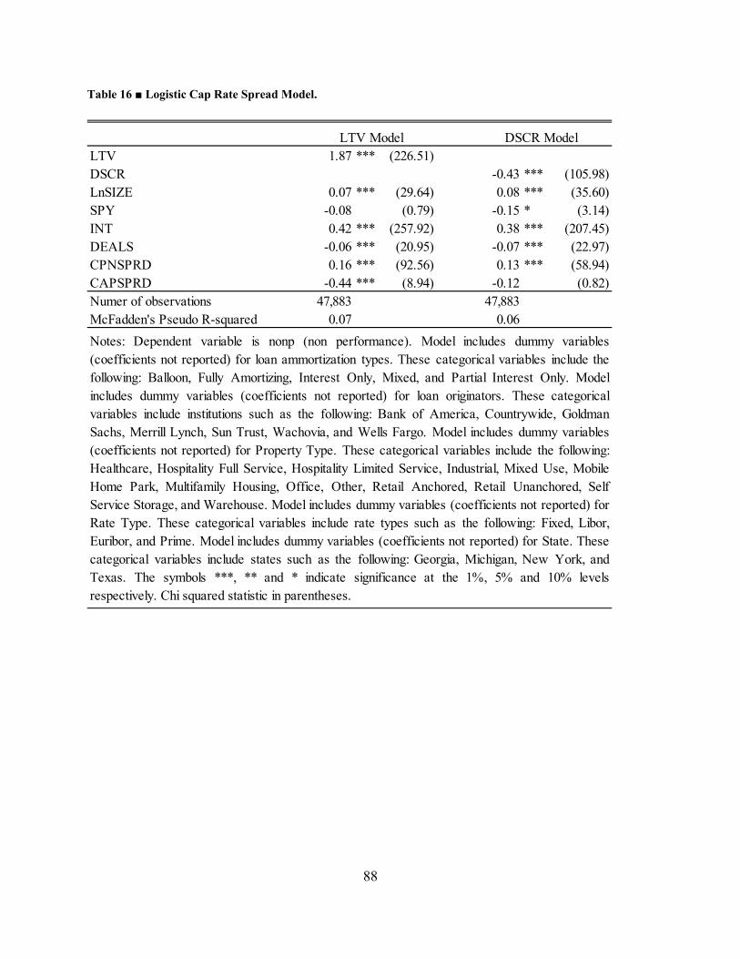
88

Table 16 ■ Logistic Cap Rate Spread Model.

LTV 1.87 *** (226.51)DSCR -0.43 *** (105.98)LnSIZE 0.07 *** (29.64) 0.08 *** (35.60)SPY -0.08 (0.79) -0.15 * (3.14)INT 0.42 *** (257.92) 0.38 *** (207.45)DEALS -0.06 *** (20.95) -0.07 *** (22.97)CPNSPRD 0.16 *** (92.56) 0.13 *** (58.94)CAPSPRD -0.44 *** (8.94) -0.12 (0.82)Numer of observations 47,883 47,883 McFadden's Pseudo R-squared 0.07 0.06

Notes: Dependent variable is nonp (non performance). Model includes dummy variables(coefficients not reported) for loan ammortization types. These categorical variables include thefollowing: Balloon, Fully Amortizing, Interest Only, Mixed, and Partial Interest Only. Modelincludes dummy variables (coefficients not reported) for loan originators. These categoricalvariables include institutions such as the following: Bank of America, Countrywide, GoldmanSachs, Merrill Lynch, Sun Trust, Wachovia, and Wells Fargo. Model includes dummy variables(coefficients not reported) for Property Type. These categorical variables include the following:Healthcare, Hospitality Full Service, Hospitality Limited Service, Industrial, Mixed Use, MobileHome Park, Multifamily Housing, Office, Other, Retail Anchored, Retail Unanchored, SelfService Storage, and Warehouse. Model includes dummy variables (coefficients not reported) forRate Type. These categorical variables include rate types such as the following: Fixed, Libor,Euribor, and Prime. Model includes dummy variables (coefficients not reported) for State. Thesecategorical variables include states such as the following: Georgia, Michigan, New York, andTexas. The symbols ***, ** and * indicate significance at the 1%, 5% and 10% levelsrespectively. Chi squared statistic in parentheses.

LTV Model DSCR Model

89

Although LTV and DSCR are correlated as expected, these variables are not the primary

variables of interest and thus may be included together in the empirical tests in order to further

improve the explanatory possibilities of the model. In addition to the robustness checks for

endogeneity of coupon rates with LTV / DSCR and the distribution assumption, select models

were modified to introduce interaction effects between LTV, DSCR, Cap Rate Spread, and

market interest rates. The result of this process provided evidence of a significant interaction

between Cap Rate Spread, and DSCR. Three models are estimated and presented with DSCR,

LTV and both in the models reported in Table 17. The interaction terms included in the models

are as follows: Cap Rate Spread with LTV, Cap Rate Spread with DSCR, LTV with DSCR, and

Cap Rate Spread with Int (10-Year Treasury yield).

In the first model with only LTV, the interaction terms for Cap Rate Spread with DSCR and

LTV with DSCR are significant. The second model which replaces LTV with DSCR, has similar

results with the same interaction terms significant yet the LTV with DSCR interaction term

reverses sign. This is likely due to the change from including LTV to including DSCR in the

model. The third model includes both LTV and DSCR and again has a significant positive result

for the Cap Rate Spread with DSCR interaction term. The LTV with DSCR term remains

significant at the 10% level and again returns to a negative sign. In this final model with LTV,

DSCR and the Cap Rate Spread with DSCR interaction term, DSCR is insignificant. Of

particular note is the result for Cap Rate Spread. This variable, the focus of other models

throughout this dissertation is insignificant in all cases when the Cap Rate Spread with DSCR

variable is included in the model. DSCR is significant at the 1% level, Cap Rate Spread is

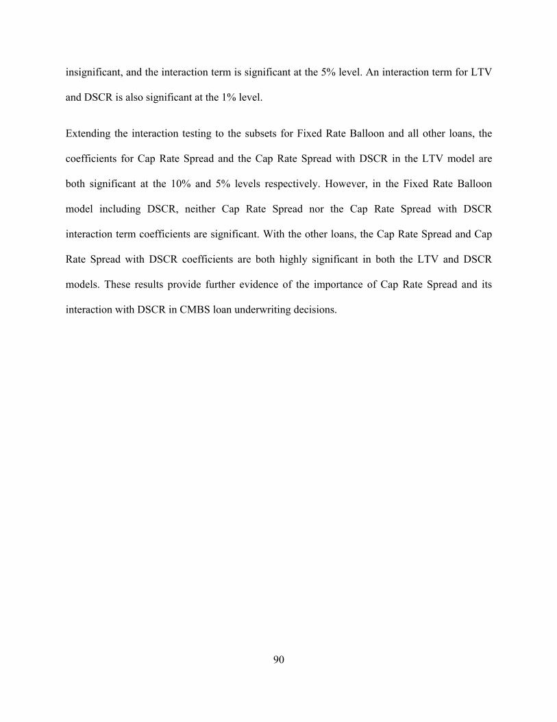
90

insignificant, and the interaction term is significant at the 5% level. An interaction term for LTV

and DSCR is also significant at the 1% level.

Extending the interaction testing to the subsets for Fixed Rate Balloon and all other loans, the

coefficients for Cap Rate Spread and the Cap Rate Spread with DSCR in the LTV model are

both significant at the 10% and 5% levels respectively. However, in the Fixed Rate Balloon

model including DSCR, neither Cap Rate Spread nor the Cap Rate Spread with DSCR

interaction term coefficients are significant. With the other loans, the Cap Rate Spread and Cap

Rate Spread with DSCR coefficients are both highly significant in both the LTV and DSCR

models. These results provide further evidence of the importance of Cap Rate Spread and its

interaction with DSCR in CMBS loan underwriting decisions.

91

Table 17 ■ Interaction Model.

Research Limitations

The study by Archer, Elmer, Harrison, and Ling (2002) discusses survivor bias, a common

problem with loan performance databases. The authors methodically present the issues of both

left- and right-censoring of their data. Left-censoring can happen when loans are paid off early or

when loans default and the property is sold prior to the observation point. As a result, these

loans, which were originated alongside other loans in the final sample, are not included in the

final sample. Similarly, databases provided by banks, insurance companies, and regulatory

LTV 1.19 *** (223.99) 1.25 *** (49.92)DSCR -0.33 *** (163.86) 0.02 (0.17)LnSIZE 0.04 *** (24.85) 0.04 *** (28.53) 0.04 *** (24.89)SPY -0.05 (.85) -0.04 (0.74) -0.05 (0.85)INT 0.24 *** (229.41) 0.25 *** (250.05) 0.24 *** (228.35)DEALS -0.04 *** (23.12) -0.04 *** (21.55) -0.04 *** (23.13)SPNSPRD 0.09 *** (79.46) 0.09 *** (77.21) 0.09 *** (79.61)CAPSPRD -0.89 (.41) -0.44 (0.10) -0.91 (0.42)CAPSPRD x LTV 0.15 (.02) 0.14 (0.01) 0.16 (0.02)CAPSPRD x DSCR 1.08 *** (12.03) 0.78 ** (6.47) 1.08 *** (12.15)LTV x DSCR -0.17 *** (7.87) 0.48 *** (75.22) -0.20 * (3.50)CAPSPRD x INT -0.20 (1.52) -0.20 (1.57) -0.19 (1.51)Numer of observations 47,883 47,883 47,883 McFadden's Pseudo R-squared 0.07 0.07 0.07

LTV and DSCR Model

Notes: Dependent variable is nonp (non performance). Model includes dummy variables (coefficients not reported) forloan originators. These categorical variables include institutions such as the following: Bank of America, Countrywide,Goldman Sachs, Merrill Lynch, Sun Trust, Wachovia, and Wells Fargo. Model includes dummy variables (coefficients notreported) for Property Type. These categorical variables include the following: Healthcare, Hospitality Full Service,Hospitality Limited Service, Industrial, Mixed Use, Mobile Home Park, Multifamily Housing, Office, Other, RetailAnchored, Retail Unanchored, Self Service Storage, and Warehouse. Model includes dummy variables (coefficients notreported) for State. These categorical variables include states such as the following: Georgia, Michigan, New York, andTexas. The symbols ***, ** and * indicate significance at the 1%, 5% and 10% levels respectively. Chi Squared statistic isin parentheses.

LTV Model DSCR Model

92

agencies are also prone to right-censoring of the data. The problem with right censoring is not

missing loans, but rather loans that are present in the sample but have not yet defaulted. These

limitations plague empirical studies in many domains that rely upon secondary data gathered and

maintained primarily for the purposes of operating an ongoing business or governmental

concern.

To reduce the effects of left-censoring, Archer, Elmer, Harrison, and Ling (2002) removed loans

from their sample that had seasoned for more than 24 months prior to securitization by the RTC

or FDIC. The authors point out that the problems of left censoring may be mitigated in the case

of a multivariate analysis since, as they postulate, the marginal effects of the default factors

likely influence the censored and uncensored loans equally.

Another typical issue with this type of data is accuracy. As a screen for the accuracy of key

variables such as LTV and DSCR, values may be assessed to identify those which may be

considered unreasonable. For example, outliers that fall far from industry standards may be

eliminated from the sample on the grounds that they are either mistakes or represent atypical

arrangements at the time of origination. For their sample, Archer, Elmer, Harrison, and Ling

(2002) set cutoff criteria for the loan contract rate, original LTV, and DSCR to eliminate the

potential effects of outliers. Although a similar process was used with this research to deal with

outliers, the nature of CMBS loans and databases which provide the sources for secondary data

research are prone to lack data and contain errors.

In one example of the potential for bias related to uncertainty in the data, the validity of

parameter estimates in models including LTV rely upon the assumption that each property is

encumbered by only one loan. If, however, some loans in the CMBS loan database are second

93

mortgages these loans may experience more stress than other loans with the same LTV where the

loan reported for the observation is the only loan for the property.

Another potential bias in the research is due to missing data. The most notable example is due to

missing or invalid values for net operating income (NOI), a variable needed to compute Cap Rate

and thus Cap Rate Spread. NOI is missing in 21,945, roughly 30% of the original sample of

73,196 U.S. loans originated starting in 1993. If this large number of loans differs from the

remaining sample in a non-random manner in characteristics related to the measured

relationships, the final results of this research may be severely biased. One possible extension of

this research would be to supplement the Bloomberg data with additional sources which would

fill in the NOI gaps and add other loan and originator data elements which may further add to the

research possibilities herein.

94

CHAPTER FIVE – NUMERICAL ANALYSIS

Applications

In practice, underwriters may be advised to select a decision rule or screening criteria related to

Cap Rate Spread that is utilized alongside LTV and DSCR when making approval and/or pricing

decisions on commercial mortgage loans. While the level selected by individual underwriters

will vary according to the business model and risk tolerance of each firm, it may be illustrative to

select a cutoff point and demonstrate the effect this prescription may have had on the rate of loan

Non-performance for past loans. For demonstration purposes, a level of 1% is selected as a

minimum Cap Rate Spread required for loans which would be approved for origination.

To ensure that the Cap Rate Spread is evaluated for its additional power to reduce loan Non-

performance, the conservative LTV and DSCR rules are first applied. To visually present the

result of increasingly restrictive underwriting criteria, a chart is constructed beginning with the

rate of Non-performance for all loans, proceeding to the level of Non-performance with the

conservative LTV and DSCR rules, and ending with the level of Non-performance by adding the

Cap Rate Spread rule. The chart displays the much reported rise in Non-performance for those

loans originated throughout the 2000s with the peak occurring in early-2007.

By introducing the LTV and DSCR criteria, the risk of Non-performance follows the same

pattern but at levels markedly lower than what actually happened. The lowest line, for the

addition of the Cap Rate Spread rule, is lower still and also demonstrates a slightly different

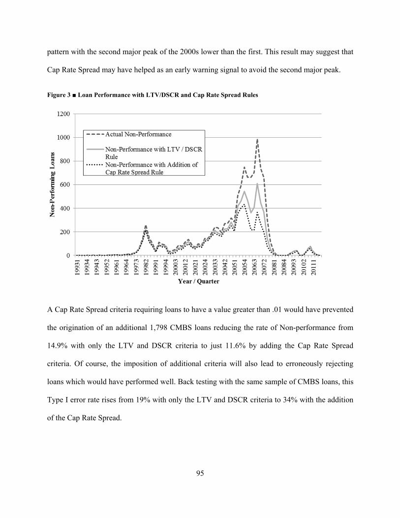
95

pattern with the second major peak of the 2000s lower than the first. This result may suggest that

Cap Rate Spread may have helped as an early warning signal to avoid the second major peak.

Figure 3 ■ Loan Performance with LTV/DSCR and Cap Rate Spread Rules

A Cap Rate Spread criteria requiring loans to have a value greater than .01 would have prevented

the origination of an additional 1,798 CMBS loans reducing the rate of Non-performance from

14.9% with only the LTV and DSCR criteria to just 11.6% by adding the Cap Rate Spread

criteria. Of course, the imposition of additional criteria will also lead to erroneously rejecting

loans which would have performed well. Back testing with the same sample of CMBS loans, this

Type I error rate rises from 19% with only the LTV and DSCR criteria to 34% with the addition

of the Cap Rate Spread.

96

Ultimately, CMBS loan underwriters must individually determine an acceptable level of Non-

performance appropriate to their business model and tolerance for risk. Using intuition,

experience, tools, and rules, each underwriter must choose a balance between the competing

risks of rejecting potentially profitable loans and accepting loans which will fail. This research

result is important because it helps deepen our understanding of the relationships between

property income and loan performance and provides an additional tool that underwriters may

employ in assessing CMBS loan risk.

97

CHAPTER SIX – CONCLUSIONS AND IMPLICATIONS FOR FUTURE

RESEARCH

Conclusions

Standard measures such as LTV and DSCR are the mainstay of commercial mortgage

underwriting risk assessment. Despite the continued reliance upon these trusted measures,

commercial mortgage Non-performance and ultimate default rose significantly during the

financial crisis of the late 2000s. This rise in defaults, coupled with a boom in the securitization

of commercial mortgages, provides motivation for studying loan and origination factors known

at origination and their relationships with future Non-performance. In this dissertation, an

additional factor is proposed that appears to have a relation to Non-performance: the Cap Rate

Spread. This spread between the unlevered rate of return on the building and the coupon rate of

the loan provides an indication of how profitable a project is to the mortgagee and how insulated

they are against shocks to their NOI. A borrower with a high Cap Rate Spread has a greater

ability to make continued loan payments during an economic downturn. Although Cap Rate

Spread and DSCR are expected to rise together in most circumstances, periods of especially low

interest rates may lead to loans with high DSCR and low Cap Rate Spread. These loans

originated during low interest rate periods may be a particular risk of Non-performance.

The use of Cap Rate Spread is demonstrated as an additional underwriting standard on those

loans which would have passed conservative criteria based on LTV and DSCR. These “safe”

loans should provide fertile ground for exploring the marginal benefit of a Cap Rate Spread

underwriting policy. Back-testing with the sample of CMBS loans originated in the 1993 – 2011

98

time period will show the quantity of loans which, though meeting the LTV and DSCR criteria,

would have been rejected on a Cap Rate Spread basis, as well as the rate of error in rejecting

loans that would have continued performing though the sample period.

The research relies primarily upon a probit methodology to estimate the parameters related to the

probability of Non-performance in a sample of 47,883 individual loans that ultimately were

packaged into CMBS. The evidence revealed through empirical testing suggests that Cap Rate

Spread does provide significant additional information beyond that of the traditional ratios of

LTV and DSCR. With the full database, results for models including LTV contained

significantly negative coefficients for Cap Rate Spread suggesting that as Cap Rate Spread

widens, the risk of Non-performance falls. When DSCR is included in the model, however, the

Cap Rate Spread coefficient is no longer significant.

With the sample split into two groups, a homogenous group of the most common loans, Fixed

Rate Balloon, and all other loans, the results for the Fixed Rate Balloon loans are consistent for

both the LTV and DSCR models. With the group of Fixed Rate Balloon loans, the coefficient for

Cap Rate Spread is negative and significant in all specifications including a two-stage model

with a Cap Rate Spread measure based on a predicted Coupon Rate. The results are also robust to

changing the distribution assumption from normal to logistic by modeling with the logit

approach rather than probit. For the group of other loans, the coefficient for Cap Rate Spread is

positive and significant in the DSCR model but is insignificant in the LTV model suggesting that

Cap Rate Spread adds no additional information beyond LTV or that the set of variables in the

model do not adequately represent the Non-performance process.

99

The final aim of this dissertation is to suggest and model the outcome of using a Cap Rate Spread

underwriting standard when evaluating and approving commercial mortgage loans. Modeling the

potential outcome of an underwriting tool such as Cap Rate Spread, an arbitrary cutoff point is

set at 1% and analyzed for the effect on originations during the sample period of requiring a

value greater than the cutoff in order for a loan to be approved. To better understand the marginal

effects of such a policy, only loans which would have also passed conservative LTV and DSCR

tests are considered. Loans that meet tests requiring LTV less than .8 and DSCR greater than

1.25 are further restricted with a Cap Rate Spread criteria that require loans to have a value

greater than 1%. Such a policy would have prevented the origination of an additional 1,798

CMBS loans reducing the rate of Non-performance from 14.9% with only the LTV and DSCR

criteria to just 11.6% by adding the Cap Rate Spread criteria.

If the null hypothesis with respect to loan performance is that loans will perform, a false positive

(Type I) error would be the equivalent of blocking the origination of a loan which would have

performed through the sample period. Back testing with the same sample of CMBS loans, this

Type I error rate rises from 19%, with only the LTV and DSCR criteria, to 34% with the addition

of the Cap Rate Spread. This prescription must be used with caution because the performance of

the loans is only known through the end of the observation period. This truncated sample period

does not include future Non-performance of the currently performing loans and thus may be

biased by loans originated in later periods which did not experience economic conditions which

may likely lead to Non-performance.

The appropriate Cap Rate Spread floor for use as an underwriting standard will necessarily vary

according to the risk-tolerance and profitability of the individual originators or the investors

100

purchasing the pools of mortgages through their CMBS shares. Loans or CMBS pools using a

Cap Rate Spread floor policy that is otherwise similar to other loans or pools may provide an

additional measure of protection against subsequent Non-performance or default. While no one

Cap Rate Spread floor would be appropriate for all originators, all originators should consider

incorporating this simple criteria into their broader program of underwriting tools.

Future Research Directions

Are there some situations where LTV, DSCR, or Cap Rate Spread is the binding constraint or the

decision rule that would override in situations where the other rules disagree as to the approval of

a loan? For example, there may be some situations when, even though the ratios LTV and DSCR

suggest a loan is too risky for origination, the loan’s Cap Rate Spread would support a favorable

origination decision. The presentation in Figure 3 shows the possibility of the reverse, loans

which would be approved on the basis of their LTV and DSCR ratios but may be declined due to

a low Cap Rate Spread. The economic conditions and loan characteristics which determine the

binding constraint from among LTV, DSCR and Cap Rate Spread is an area for further

investigation. Visual inspection of the trends in levels seems to indicate that the relationship

between interest rates and Cap Rate Spread changed after 2007. This potential structural break

warrants further study to understand whether this apparent change is significant and to test

theories which may explain the change, if any, to this relationship.

As pointed out previously, a simple rule to block the origination of loans likely to experience

trouble in the future must be combined with information needed to balance the potential profits

of lending with the potential losses of loan defaults. Any decision rule is likely to reject loans

101

which would have performed well and accept loans which will later default. Research combining

the profitability of particular loans or general loan characteristics with the institutional costs of

default may help illuminate this interesting but unexplored aspect of loan performance and

default. Extending this research to include additional information about the loan originators such

as type of firm, extent to which originators retain an equity stake in target CMBS, and depth and

experience of underwriting organizations may further demonstrate the importance of Cap Rate

Spread in predicting CMBS loan performance.

102

REFERENCES

Ambrose, BW, and AB Sanders. 2003. Commercial Mortgage-Backed Securities: Prepayment and Default. The Journal of Real Estate Finance and Economics 26: 179-196.

An, X, Y Deng, and AB Sanders. 2010. Default Risk of CMBS Loans: What Explains the Regional Variations? Working Paper.

An, X, and AB Sanders. 2010. Default of Commercial Mortgage Loans during the Financial Crisis. 2010 AREUEA Mid-Year Conference.

Archer, WR, PJ Elmer, DM Harrison, and DC Ling. 2002. Determinants of Multifamily Mortgage Default. Real Estate Economics 30: 445-473.

Black, LK, CS Chu, AM Cohen, and J Nichols. 2011. Differences Across Originators in CMBS Loan Underwriting. Finance and Economics Discussion Series, Federal Reserve Board: Washington DC.

Bliss, CI. 1935. The Calculation of the Dosage-Mortality Curve. Annals of Applied Biology 22: 134-167.

Bollen, KA, and R Jackman. 1990. Regression diagnostics: An expository treatment of outliers and influential cases. JFJS Long, editor Modern Methods of Data Analysis, Sage: Newbury Park.

Chen, J, and Y Deng. 2010. Commercial Mortgage Workout Strategy and Conditional Default Probability: Evidence from Special Serviced CMBS Loans. NUS Institute of Real Estate Studies Working Paper, National University of Singapore.

Childs, PD, SH Ott, and TJ Riddiough. 1996. The Pricing of Multiclass Commercial Mortgage-Backed Securities. The Journal of Financial and Quantitative Analysis Vol. 31: 581-603.

Christopoulos, AD, RA Jarrow, and Y Yildirim. 2008. Commercial Mortgage-Backed Securities (CMBS) and Market Efficiency with Respect to Costly Information. Real Estate Economics 36: 441-498.

Ciochetti, BA, Y Deng, G Lee, JD Shilling, and R Yao. 2003. A Proportional Hazards Model of Commercial Mortgage Default with Originator Bias. The Journal of Real Estate Finance and Economics 27: 5-23.

Cook, RD, and S Weisberg. 1982. Residuals and influence in regression. Chapman & Hall: New York.

Corcoran, PJ. 2009. Commercial Mortgage Default and Refinancing Risk: A Primer The Journal of Portfolio Management Vol. 35: 70-79.

103

De Leonardis, D, and R Rocci. 2008. Assessing the default risk by means of a discrete-time survival analysis approach. Applied Stochastic Models in Business and Industry 24: 291-306.

Deng, Y, SA Gabriel, and AB Sanders. 2011. CDO market implosion and the pricing of subprime mortgage-backed securities. Journal of Housing Economics 20: 68-80.

Downing, C, R Stanton, and N Wallace. 2008. Volatility, Mortgage Default, and CMBS Subordination. Working Paper.

Finney, DJ. 1952. Probit Analysis. Cambridge University Press: Cambridge, England.

Finney, DJ, and WL Stevens. 1948. A table for the calculation of working probits and weights in probit analysis. Biometrika 35: 191-201.

Furfine, C. 2011. Deal Complexity, Loan Performance, and the Pricing of Commercial Mortgage Backed Securities. Working Paper.

Gallo, JG, RJ Buttimer, LJ Lockwood, and RC Rutherford. 1997. Determinants of Performance for Mortgage-Backed Securities Funds. Real Estate Economics 25: 657-681.

Goldberg, L, and CA Capone, Jr. 1998. Multifamily Mortgage Credit Risk: Lessons From Recent History. Cityscape 4.

Goldberg, L, and CA Capone, Jr. 2002. A Dynamic Double-Trigger Model of Multifamily Mortgage Default. Real Estate Economics 30: 85-113.

Greenberg, BG. 1980. Chester I. Bliss, 1899-1979. International Statistical Review / Revue Internationale de Statistique 8: 135-136.

Grovenstein, RA, JP Harding, CF Sirmans, S Thebpanya, and GK Turnbull. 2005. Commercial mortgage underwriting: How well do lenders manage the risks? Journal of Housing Economics 14: 355-383.

Hahn, ED, and R Soyer. 2005. Probit and Logit Models: Differences in a Multivariate Realm. Working Paper, Retrieved Oct 17, 2011 from http://home.gwu.edu/~soyer/mv1h.pdf.

Holford, TR, and C White. 2005. Bliss, Chester Ittner. Encyclopedia of Biostatistics, John Wiley & Sons, Ltd.

Kau, J, D Keenan, and Y Yildirim. 2009. Estimating Default Probabilities Implicit in Commercial Mortgage Backed Securities (CMBS). The Journal of Real Estate Finance and Economics 39: 107-117.

Kau, JB, DC Keenan, WJ Muller III, and JF Epperson. 1987. The Valuation and Securitization of Commercial and Multifamily Mortgages. Journal of Banking & Finance 11: 525-546.

Pampel, FC. 2000. Logisitc Regression, A Primer. Sage.

104

Schneider-Orelli, O. 1947. Entomologisches Pratikum. HR Sauerländer and Co: Aarau.

Seslen, T, and WC Wheaton. 2010. Contemporaneous Loan Stress and Termination Risk in the CMBS Pool: How “Ruthless” is Default? Real Estate Economics 38: 225-255.

Titman, S, and W Torous. 1989. Valuing commercial mortgages: An empirical investigation of the contingent claims approach to pricing risky debt. Journal of Finance 44: 345-373.

Titman, S, and S Tsyplakov. 2010. Originator Performance, CMBS Structures, and the Risk of Commercial Mortgages. Review of Financial Studies 23: 3558-3594.

UCLA-ATS. 2011. Statistical Computing - Frequently Asked Questions. Accessed on December 19, 2011. http://www.ats.ucla.edu/stat/mult_pkg/faq/general/citingats.htm UCLA: Academic Technology Services, Statistical Consulting Group.

Vandell, KD. 1984. On the Assessment of Default Risk in Commercial Mortgage Lending. AREUEA Journal: Journal of the American Real Estate & Urban Economics Association 12: 270-296.

—. 1992. Predicting Commercial Mortgage Foreclosure Experience. Real Estate Economics 20: 55-88.

Vincent, K. 2008. Probit Analysis. Accessed on February 2, 2012. http://userwww.sfsu.edu/~efc/classes/biol710/probit/ProbitAnalysis.pdf.

Xu, XE, and H-G Fung. 2005. What Moves the Mortgage-Backed Securities Market? Real Estate Economics 33: 397-426.

Yildirim, Y. 2008. Estimating Default Probabilities of CMBS Loans with Clustering and Heavy Censoring. The Journal of Real Estate Finance and Economics 37: 93-111.