
A Multi-Agent Design for Smart Distribution Automation ...
170
Graduate Theses, Dissertations, and Problem Reports 2017 A Multi-Agent Design for Smart Distribution Automation System A Multi-Agent Design for Smart Distribution Automation System with Distributed Energy Resources and Microgrids with Distributed Energy Resources and Microgrids Sridhar Chouhan Follow this and additional works at: https://researchrepository.wvu.edu/etd Recommended Citation Recommended Citation Chouhan, Sridhar, "A Multi-Agent Design for Smart Distribution Automation System with Distributed Energy Resources and Microgrids" (2017). Graduate Theses, Dissertations, and Problem Reports. 5363. https://researchrepository.wvu.edu/etd/5363 This Dissertation is protected by copyright and/or related rights. It has been brought to you by the The Research Repository @ WVU with permission from the rights-holder(s). You are free to use this Dissertation in any way that is permitted by the copyright and related rights legislation that applies to your use. For other uses you must obtain permission from the rights-holder(s) directly, unless additional rights are indicated by a Creative Commons license in the record and/ or on the work itself. This Dissertation has been accepted for inclusion in WVU Graduate Theses, Dissertations, and Problem Reports collection by an authorized administrator of The Research Repository @ WVU. For more information, please contact [email protected].
Transcript of A Multi-Agent Design for Smart Distribution Automation ...

Graduate Theses, Dissertations, and Problem Reports
2017
A Multi-Agent Design for Smart Distribution Automation System A Multi-Agent Design for Smart Distribution Automation System
with Distributed Energy Resources and Microgrids with Distributed Energy Resources and Microgrids
Sridhar Chouhan
Follow this and additional works at: https://researchrepository.wvu.edu/etd
Recommended Citation Recommended Citation Chouhan, Sridhar, "A Multi-Agent Design for Smart Distribution Automation System with Distributed Energy Resources and Microgrids" (2017). Graduate Theses, Dissertations, and Problem Reports. 5363. https://researchrepository.wvu.edu/etd/5363
This Dissertation is protected by copyright and/or related rights. It has been brought to you by the The Research Repository @ WVU with permission from the rights-holder(s). You are free to use this Dissertation in any way that is permitted by the copyright and related rights legislation that applies to your use. For other uses you must obtain permission from the rights-holder(s) directly, unless additional rights are indicated by a Creative Commons license in the record and/ or on the work itself. This Dissertation has been accepted for inclusion in WVU Graduate Theses, Dissertations, and Problem Reports collection by an authorized administrator of The Research Repository @ WVU. For more information, please contact [email protected].
A Multi-Agent Design for Smart Distribution
Automation System with Distributed Energy
Resources and Microgrids
Sridhar Chouhan
Dissertation submitted to the
Benjamin M. Statler College of Engineering and Mineral Resources
at West Virginia University
in partial fulfillment of the requirements for the degree of
Doctor of Philosophy in Electrical Engineering
Ali Feliachi, Ph.D., Chair
M. A. Choudhry, Ph.D.
Sarika Khushalani Solanki, Ph.D.
Powsiri Klinkhachorn, Ph.D.
Daryl S Reynolds, Ph.D.
Hong-Jian Lai, Ph.D.
Lane Department of Computer Science and Electrical Engineering
Morgantown, West Virginia
2017
Keywords: Multi-Agent System, Distribution Automation, Fault Location and Isolation,
Service Restoration, Distributed Energy Resources, Microgrids, Reinforcement Learning,
Switch Optimization
Copyright 2017 Sridhar Chouhan

ABSTRACT
A Multi-Agent Design for Smart Distribution Automation System
with Distributed Energy Resources and Microgrids
Sridhar Chouhan
The proliferation of Smart Grid technologies such as distributed energy resources (DER) and microgrids
has resulted in new opportunities and challenges to existing Distribution Automation (DA) solutions. A
novel hybrid Multi-Agent System (MAS) Fault Location, Isolation, and Restoration (FLIR) solution is
proposed for electric distribution systems with different types of distributed generation (DG) resources and
microgrids. The main goal of the MAS is to locate and isolate the fault and then to automatically reenergize
fault-free portions of the network to restore power to as many customers as possible while maintaining
system constraints like voltage and thermal capacity limits.
Determination of the optimum number and placement of automated switches is an important and a daunting
task in the economic feasibility process of any DA project. An innovative algorithm based on relative
reduction in the normalized customer interruption costs is presented for the switch optimization problem.
The proposed approach isolates the impacts of varying switch investment and customer interruption costs
that are usually based on outdated surveys.
A distributed Fault Detection algorithm is presented to support sectionalizing switch agents (SSA) to
autonomously detect the fault condition and type of the fault by using the local data such as voltage and
current phasor measurements. Fault characteristics of various DG systems including inverter based DG,
synchronous generator, and induction generator are considered in the proposed algorithm. Fault isolation
and service restoration functionalities are achieved through coordinated communications among the agents
using both centralized and decentralized control strategies. Feeder Agent (FA) uses the proposed “Tie-
Switch Ranking Algorithm” and “Zone Priority Algorithm” to solve the service restoration problem. A new
reinforcement agent learning mechanism based on Q-learning is introduced to support FAs with service
restoration task.
The proposed MAS is designed to be demonstrated on Mon Power, a FirstEnergy company, distribution
system as part of the DOE project, West Virginia Super Circuit (WVSC). The actual distribution network
is simulated using CYME®, Matlab®/Simpower®, and PSCAD® software, whereas the MAS and its
communications are simulated using Matlab® S-functions. The switch optimization results show that the
proposed iterative algorithm can drastically reduce the search space, and can find optimal number and
placement of the switches with minimum computational effort. The FLIR simulation results show
promising advantages of using the proposed MAS solution with the agent learning capabilities for fault
location and service restoration tasks.

iii
The only living gods on earth are,
‘Parents’

iv
Acknowledgements
After several years of my PhD program, I have learned one thing – I could never have completed
my dissertation, without the support and encouragement of many people around me. First of all, I
would like to thank my esteemed mentor and advisor, Dr. Ali Feliachi. He has given me a chance
to continue my work in the field of power systems to pursue my passion. It was a blessing to be
one of his students and be able to conduct research with him. I would also like to thank rest of my
committee, Dr. Muhammad A. Choudhry, Dr. Sarika Khushalani Solanki, Dr. Powsiri
Klinkhachorn, Dr. Daryl S Reynolds, and Dr. Hong-Jian Lai for their constructive comments. My
sincere thanks go to Dr. Kevin Milans for his feedback. Their guidance helped me immensely to
shape and improve my research as well as my dissertation document.
I would like to extend my thanks to Mon Power, a FirstEnergy Company, especially to Mr. Harley
Mayfield, for providing the distribution system data to help with my research work.
I would like to thank my family and in-laws for their unending support and love. Without their
support, I couldn’t have made it through this process. My sincere gratitude goes to my cousin for
helping and motivating me. I can never thank enough to my loving wife for all her support and
understanding, she sacrificed countless weekends to help me get this degree. My humble pranam
goes to the almighty god for being always with me as a guiding light.
Lastly, Grand Pa, I miss you so much!!!
v
Contents
ABSTRACT ................................................................................................................................... ii
Acknowledgements ...................................................................................................................... iv
Contents ......................................................................................................................................... v
List of Figures ............................................................................................................................... ix
List of Tables ............................................................................................................................... xii
Nomenclature ............................................................................................................................. xiii
Symbols ....................................................................................................................................... xiv
Chapter 1 Introduction ............................................................................................................... 1
1.1 Problem Statement ........................................................................................................................... 3
1.2 Approach .......................................................................................................................................... 6
1.3 Contributions ................................................................................................................................... 8
1.4 Dissertation Outline ......................................................................................................................... 9
1.5 Publications .................................................................................................................................... 10
Chapter 2 Literature Review ................................................................................................... 11
2.1 Multi-Agent Systems ..................................................................................................................... 11
2.2 Switch Optimization ...................................................................................................................... 12
2.3 Fault Location and Isolation .......................................................................................................... 14
2.4 Service Restoration ........................................................................................................................ 16
2.4.1 Expert Systems and Heuristics ............................................................................................ 17
2.4.2 Mathematical Programming ................................................................................................ 17
2.4.3 Multi-Agent System technology ......................................................................................... 18
2.5 Agent Learning .............................................................................................................................. 20
2.6 Existing FLIR Systems .................................................................................................................. 21
2.6.1 IntelliTeam SG .................................................................................................................... 22
2.6.2 IntelliTeam Working Principle ........................................................................................... 22
2.6.3 FLIR & IntelliTeam ............................................................................................................ 25

vi
Chapter 3 Multi-Agent Systems .............................................................................................. 26
3.1 Agent Communication ................................................................................................................... 30
3.1.1 FIPA-ACL ........................................................................................................................... 31
3.1.2 KQML ................................................................................................................................. 33
Chapter 4 MAS FLIR System Design ..................................................................................... 35
4.1 Proposed MAS Architecture .......................................................................................................... 35
4.1.1 Agents ................................................................................................................................. 36
4.1.1.1 Substation Agent (SA) ................................................................................................ 37
4.1.1.2 Feeder Agent (FA) ...................................................................................................... 37
4.1.1.3 Sectionalizing Switch Agent (SSA) ............................................................................ 38
4.1.1.4 Tie Switch Agent (TSA) ............................................................................................. 38
4.1.1.5 PCC Agent (PA) .......................................................................................................... 38
4.2 WVSC MAS Design ...................................................................................................................... 41
4.3 Agent State Transition ................................................................................................................... 42
4.4 Proposed FLIR Process Flow ......................................................................................................... 43
Chapter 5 Switch Optimization ............................................................................................... 45
5.1 Mathematical Problem Formulation .............................................................................................. 46
5.2 Iterative Algorithm for Optimal Switch Number and Placement .................................................. 47
5.3 Test System and Results ................................................................................................................ 49
5.3.1 Test System (IEEE 34-Bus System) ................................................................................... 49
5.3.2 Test System (IEEE 123-Bus System) ................................................................................. 51
5.3.3 Test System (WVSC Distribution System) ......................................................................... 51
5.3.4 Data Assumptions ............................................................................................................... 55
5.3.5 Results ................................................................................................................................. 55
Chapter 6 DG Fault Characteristics ........................................................................................ 59
6.1 Short Circuit Analysis .................................................................................................................... 60
6.2 Synchronous Machine Fault Response .......................................................................................... 61
6.3 Induction Machine Fault Response ................................................................................................ 62
6.4 Inverter based DG Fault Response ................................................................................................ 63
6.4.1 Inverter based DG ............................................................................................................... 63
6.4.2 Inverter Control ................................................................................................................... 64
6.4.2.1 Inverter Voltage-mode Control ................................................................................... 64
6.4.2.2 Inverter Current-mode Control ................................................................................... 65
6.4.3 Fault Characteristics and Model of Inverter ........................................................................ 68
Chapter 7 MAS Fault Location & Isolation ........................................................................... 71

vii
7.1 Fault Detection Algorithm ............................................................................................................. 73
7.1.1 Loss of Voltage (LOV) Detection ....................................................................................... 74
7.1.2 Zone Over Current (ZC) Detection ..................................................................................... 74
7.1.3 Over Current Fault Detection .............................................................................................. 76
7.1.4 Permanent Fault Determination .......................................................................................... 77
7.2 Test System and Modeling ............................................................................................................. 77
7.2.1 West Virginia Super Circuit (Base Case)............................................................................ 78
7.2.1.1 Automated Switches ................................................................................................... 79
7.2.1.2 Substation Reclosers ................................................................................................... 79
7.2.1.3 Communication Architecture ...................................................................................... 80
7.2.2 West Virginia Super Circuit (FLI Test Case) ..................................................................... 81
7.2.3 PSCAD Detailed Modeling ................................................................................................. 82
7.2.3.1 PV Inverter Model ...................................................................................................... 83
7.2.3.2 Synchronous Generator Model ................................................................................... 84
7.2.3.3 Induction Generator Model ......................................................................................... 85
7.3 Fault Location & Isolation Results ................................................................................................ 86
7.3.1 Case I - Three Phase Fault in Zone-2 .................................................................................. 86
7.3.2 Case II - Line to Ground (LG-A) Fault in Zone-1 .............................................................. 93
7.3.3 Miscellaneous Faults ......................................................................................................... 100
Chapter 8 MAS Service Restoration ..................................................................................... 102
8.1 Restoration Formulation .............................................................................................................. 104
8.2 TSW Ranking Algorithm (TRA) ................................................................................................. 109
8.3 Zone Priority Algorithm (ZPA) ................................................................................................... 111
8.4 Multi-agent Logic for Return to Normal...................................................................................... 113
Chapter 9 Reinforcement Agent Learning ........................................................................... 115
9.1 Q-Learning ................................................................................................................................... 116
9.1.1 Learning ............................................................................................................................ 117
9.1.2 Exploration ........................................................................................................................ 117
9.2 Learning Methodology for Service Restoration ........................................................................... 118
9.2.1 Reinforcement Reward Function ...................................................................................... 118
9.2.2 Q-Value Matrix ................................................................................................................. 120
9.2.3 Q-Update Rule .................................................................................................................. 121
9.2.4 Action Selection Strategy .................................................................................................. 121
9.2.5 Q-Learning Process Flow .................................................................................................. 122
Chapter 10 Service Restoration Results ............................................................................... 124

viii
10.1 WVSC System (Base Case) ..................................................................................................... 124
10.2 WVSC System (Service Restoration Case) ............................................................................. 125
10.3 Power System Model ............................................................................................................... 126
10.4 MAS Model ............................................................................................................................. 128
10.5 Service Restoration Results ..................................................................................................... 128
10.5.1 Case I - Fault in Zone-0 .................................................................................................... 128
10.5.1.1 Optimization Approach ............................................................................................. 128
10.5.1.2 Agent Learning Approach ......................................................................................... 131
10.5.2 Case II - Fault in Zone-2 ................................................................................................... 133
10.6 Performance Evaluation .......................................................................................................... 135
10.6.1 Agent Communications ..................................................................................................... 135
10.6.2 Load Power Restoration .................................................................................................... 137
10.6.3 Tie-switch Operations ....................................................................................................... 138
10.6.4 Line Losses ....................................................................................................................... 139
10.6.5 Voltage Drop ..................................................................................................................... 140
Chapter 11 Conclusions and Future Work .......................................................................... 142
11.1 Conclusions ............................................................................................................................. 142
11.2 Future Work ............................................................................................................................. 146
Bibliography .............................................................................................................................. 148

ix
List of Figures
Figure 1-1: Outage Restoration without and with Distribution Automation ................................................ 3
Figure 2-1: An Example of IntelliTEAM Implementation ......................................................................... 23
Figure 3-1: Multi-Agent System for Electric Distribution System ............................................................. 27
Figure 3-2: FIPA ACL Message [66] ......................................................................................................... 32
Figure 3-3: KQML Communication Protocol [13] ..................................................................................... 34
Figure 4-1: Proposed Hybrid MAS Architecture ........................................................................................ 36
Figure 4-2: Agent Functionality Diagram ................................................................................................... 39
Figure 4-3: Agent Placement for WVSC Distribution System ................................................................... 41
Figure 4-4: Agent State Transition.............................................................................................................. 42
Figure 4-5: Proposed FLIR Process Flow ................................................................................................... 44
Figure 5-1: Typical Radial Distribution Feeder .......................................................................................... 47
Figure 5-2: Iterative Algorithm for Optimal Switch Number and Placement ............................................. 48
Figure 5-3: IEEE 34-Bus Test Feeder ......................................................................................................... 50
Figure 5-4: IEEE 123-Bus Test Feeder ....................................................................................................... 51
Figure 5-5: Geographic View of WVSC Feeders ....................................................................................... 52
Figure 5-6. WR#3 and WR#4 Distribution Transformer Data ................................................................... 53
Figure 5-7: Customer Damage Functions ................................................................................................... 55
Figure 5-8: Calculated Indices for IEEE 34-Bus, IEEE-123 Bus, WR#3, and WR#4 Feeders .................. 56
Figure 5-9: Comparison of CIC Calculations between Traditional [67] and Proposed Approaches .......... 58
Figure 6-1: Circuit Model for Asymmetrical Fault Current ........................................................................ 60
Figure 6-2: Short Circuit Asymmetrical Current [70]................................................................................. 61
Figure 6-3: Synchronous Machine Response to Three Phase Fault ............................................................ 62
Figure 6-4: Induction Machine Response to Three Phase Fault ................................................................. 63
Figure 6-5: Inverter based DG .................................................................................................................... 64
Figure 6-6: Grid-connected Inverter Voltage-mode Control ...................................................................... 65
Figure 6-7: Grid-connected Inverter Current-mode Control ....................................................................... 66

x
Figure 6-8: Power Controller Implementation ............................................................................................ 67
Figure 6-9: Fault Response of an Inverter under Current-mode Control .................................................... 69
Figure 6-10: Equivalent Circuit of Grid-connected Inverter with Current Limiting .................................. 70
Figure 6-11: Equivalent Sequence Network of Grid-connected Inverter ................................................... 70
Figure 7-1: Agent Communication for Fault Location and Isolation.......................................................... 72
Figure 7-2: Fault Detection Algorithm Blocks ........................................................................................... 73
Figure 7-3: Fault Detection Algorithm – Voltage and Zone Current Change Waveforms ......................... 76
Figure 7-4: AND Gate Implementation of Over Current Fault Detection .................................................. 77
Figure 7-5: Single Line Diagram of WVSC Project 12.5 kV Circuits ........................................................ 78
Figure 7-6: Pole-top Load Break Switch .................................................................................................... 79
Figure 7-7: Recloser with Cooper Form-6 Controller at WestRun Substation ........................................... 80
Figure 7-8: Simplified One Line Diagram of WVSC Feeders for MAS FLI ............................................. 82
Figure 7-9: WVSC Distribution Feeder WR#3 PSCAD Model ................................................................. 83
Figure 7-10: PSCAD Model of PV Inverter ............................................................................................... 84
Figure 7-11: Synchronous Generator PSCAD Model ................................................................................. 85
Figure 7-12: Induction Generator PSCAD Model ...................................................................................... 86
Figure 7-13: DG Real and Reactive Power Outputs ................................................................................... 89
Figure 7-14: DG Instantaneous Fault Contributions ................................................................................... 90
Figure 7-15: SSW3 Measurements (Voltages, Zone Current Change, Fault Flag, and Permanent Fault
Flag) ............................................................................................................................................................ 91
Figure 7-16: Instantaneous Voltages at the Substation and SSW locations ................................................ 92
Figure 7-17: Agent Communications for Fault Location and Isolation for LLL Fault in Zone-2 .............. 93
Figure 7-18: DG Real and Reactive Power Outputs ................................................................................... 96
Figure 7-19: DG Instantaneous Fault Contributions ................................................................................... 97
Figure 7-20: SSW1 Measurements (Voltages, Zone Current Change, Fault Flag, and Permanent Fault
Flag) ............................................................................................................................................................ 98
Figure 7-21: Instantaneous Voltages at the Substation and SSW locations ................................................ 99
Figure 7-22: Agent Communications for Fault Location and Isolation for LG-A Fault in Zone-1 .......... 100
Figure 8-1: Typical Radial Distribution Feeder with Super Zones ........................................................... 103
Figure 8-2: Service Restoration of Super Zone-A .................................................................................... 104
Figure 8-3: Service Restoration of Super Zone-B .................................................................................... 108
Figure 8-4: Typical Configuration of Distribution System ....................................................................... 109
Figure 8-5: Zone Energizing Sequence using Zone Priority Algorithm. .................................................. 112
Figure 8-6: MAS Logic for Return to Normal .......................................................................................... 114

xi
Figure 9-1: Q-Learning Process Flow for Service Restoration ................................................................. 123
Figure 10-1: Simplified One Line Diagram of WVSC Feeders for MAS Service Restoration ................ 126
Figure 10-2: CYME® and Matlab® Model for WVSC Project Feeders .................................................... 127
Figure 10-3: Agent Communications for Service Restoration for Zone-0 Fault ...................................... 131
Figure 10-4: Service Restorations for Case I and Case II ......................................................................... 134

xii
List of Tables
Table 2-1: SWOT Matrix for Current Agent Applications to Power Systems [14] .................................... 12
Table 3-1: FIPA ACL Message Parameters [66] ........................................................................................ 32
Table 4-1: Agent Knowledge/Capabilities and Behaviors .......................................................................... 39
Table 5-1: IEEE 34-Bus and 123-Bus Test Feeder SS Data ....................................................................... 50
Table 5-2. Reliability Indices of WVSC Circuits (Major Events Included) ............................................... 53
Table 5-3: WR#3 and WR#4 Feeder SS Data ............................................................................................. 54
Table 5-4: Calculated Indices for IEEE 34-Bus, IEEE-123 Bus, WR#3, and WR#4 Feeders .................... 57
Table 7-1: Recloser Settings ....................................................................................................................... 80
Table 7-2: Interconnection System Response to Abnormal Voltages (rms Voltage) ................................. 84
Table 7-3: Interconnection System Response to Abnormal Frequencies ................................................... 84
Table 7-4: DG Output Power and Fault Contribution ................................................................................. 88
Table 7-5: Fault Counter Value and Permanent Fault Flag Status for LLL Fault in Zone-2 ...................... 88
Table 7-6: DG Output Power and Fault Contribution ................................................................................. 95
Table 7-7: Fault Counter Value and Permanent Fault Flag Status for LG-A fault in Zone-1..................... 95
Table 7-8: Fault Location Results for Miscellaneous Faults .................................................................... 101
Table 10-1: Peak Load Data of WVSC Feeders ....................................................................................... 125
Table 10-2: Zone Pre-fault Loadings and Generation Values in CYME® ................................................ 129
Table 10-3: TSW Ranking Based on TRA ............................................................................................... 129
Table 10-4: Number of Agent Communications ....................................................................................... 137
Table 10-5: Amount of Load Power Restoration ...................................................................................... 138
Table 10-6: Tie-switch Operations ........................................................................................................... 139
Table 10-7: Line Losses ............................................................................................................................ 140
Table 10-8: Voltage Drop ......................................................................................................................... 141

xiii
Nomenclature
ACL Agent Communication Language
CAIDI Customer Average Interruption Duration Index
CB Circuit Breaker
CC Current Change
CIC Customer Interruption Cost
CMI Customer Minute Interruptions
DA Distribution Automation
DOE Department of Energy
DG Distributed Generation
EDS Electric Distribution System
FA Feeder Agent
FLI Fault Location, Isolation
FLIR Fault Location, Isolation & Restoration
KQML Knowledge Query and Manipulation Language
LOV Loss of Voltage
MAS Multi Agent System
NETL National Energy Technology Laboratory
NEZ Non-Energized Zone
OC Over-Current
OLTC On-Load Tap Changers
PA PCC Agent
PCC Point of Common Coupling
SA Substation Agent
SAIDI System Average Interruption Duration Index
SAIFI System Average Interruption Frequency Index
SCADA Supervisory Control and Data Acquisition
SSA Sectionalizing Switch Agent
SSW Sectionalizing Switch
TCC Time Current Characteristic
TSA Tie Switch Agent
TSW Tie Switch
TRA Tie-Switch Ranking Algorithm
WVSC West Virginia Super Circuit
ZPA Zone Priority Algorithm

xiv
Symbols
𝑉 voltage V (Volt)
𝐼 current A (Ampere)
𝑃 active power W (J/s)
𝑄 reactive power var
𝑡 time s (second)
𝜉 failure rate failures/mile-year
𝑓 frequency Hz
𝛽 load priority
𝑋′ transient reactance Ω (Ohms)
𝑋′′ sub-transient reactance Ω (Ohms)
𝑎 action
𝑠 state
𝛼 learning rate
𝑅 reward function

1
Chapter 1
Introduction
According to the U.S. Department of Energy (DOE), the “Smart grid” generally refers to a class
of technology that brings utility electricity delivery systems into the 21st century, using computer-
based remote control and automation [1]. The National Energy Technology Laboratory (NETL) in
the United States has presented seven principle characteristics of a smart grid [2]. The smart grid
should be able to heal itself after a power system event; it should enable active customer
participation, resist attacks, provide power quality for the 21st century needs, accommodate all
generation and storage options, enable markets, and optimize asset utilization and operate
efficiently. Among them "Self-healing" is the key characteristic. "Self-healing" in the literature
was also interpreted as a technology that enables the faulty part of a system to be isolated and,
ideally, restored to normal operation with little or no human intervention.
Supplying reliable and high quality electric power to customers is the highest priority of electric
utilities. Electric utilities employ smart technologies and advanced communications to monitor
and control the transmission and generation facilities, whereas the distribution systems are still
catching up with that level of sophistication. This was mainly due to the un-justified economics of
deploying automation technologies on the Electric Distribution System (EDS).
According to the DOE, more than 80% of outages are directly related to distribution systems which
cost the nation more than 80 billion dollars annually [3]. Utility companies are concerned about
distribution outages and its impact on their customers. Distribution system automation
technologies, especially the automated Fault Location, Isolation, and Restoration (FLIR) systems

Chapter 1. Introduction 2
can help to improve the overall system reliability and operational efficiency by minimizing the
duration and frequency of outages.
Although manual methods of fault restoration have been used for years to provide certain levels
of reliability in the EDS, automated FLIR systems can provide increased levels of reliability. Even
in today’s advanced world, most of the electric utilities still depend on customer calls to find out
outages in their systems. The field crews are dispatched to patrol the faulted lines to find out the
exact fault location and fix the fault. This is a manual intensive process and takes hours together
for fault location and isolation activities as crews sometimes have to travel tens of miles and that
to in inclement weather conditions most of the times. This is a poor way of handling fault situations
and field crews. These inefficient manual operations can cause increased outage durations and
number of outages, which can significantly hinder the system reliability.
The automated FLIR systems that exist today can locate and isolate the fault, and reconfigure the
un-faulty portion of the circuits within a couple of minutes. These FLIR systems can totally be
automated and do not require any human intervention to run. This will significantly improve the
system reliability and the relevant reliability indices (SAIFI, SAIDI, and CAIDI). Figure 1-1
illustrates how a typical outage restoration scenario might progress both with and without
advanced distribution automation [4]. The times shown will be extended even further during storm
conditions when dispatchers are juggling multiple outage investigations. Feeder automation is the
essential requirement of automated FLIR systems. The major components of feeder automation
are Supervisory Control and Data Acquisition (SCADA), automated Sectionalizing Switches
(SSW) and Tie Switches (TSW), reclosers, and advanced communications.

Chapter 1. Introduction 3
Figure 1-1: Outage Restoration without and with Distribution Automation
1.1 Problem Statement
Distribution self-healing through FLIR systems is not a new concept, but previous system designs
must be re-evaluated to ensure proper operation with the new technologies on the distribution
systems such as distributed energy resources including microgrid systems, intelligent demand
control, and Volt/VAr control systems. These new technologies pose new challenges and offer
new opportunities for improved performance of FLIR systems during emergencies.
Electric distribution facilities are routinely loaded to more than 50 percent of rated capacity, and
sufficient capacity may not be available through adjacent feeders when needed. Hence, the recent
generation of FLIR systems commonly includes a logic for dealing with these issues. Many
systems of the past decade will automatically block any load transfer that would overload adjacent
feeders. There is a clear need for more advanced FLIR systems that can divide the load into smaller
Chapter 1. Introduction 4
pieces and can be supplied by multiple adjacent feeders without violating any voltage and capacity
constraints and preferably in an optimal manner.
Some electric utilities have experienced problems with the FLIR systems that have operated
successfully for years. Often these problems are the result of increased Distributed Generation
(DG) penetration on the feeder. The fault contribution from the DG units can impact the existing
protection and coordination of the system. As a result, the protection system might locate the fault
incorrectly, and restoration switching activities may re-energize the fault and possibly lock out
multiple feeders. This problem can be addressed by using “directional” fault location logic that
identify the direction of current flow or by using centralized modeling approaches that account for
short circuit contributions from distributed generators.
Another challenge resulting from the presence of distributed generators is what is referred to herein
as the “net load” problem [5]. Present FLIR systems continuously monitor the power flowing into
and out of each feeder section to determine the load that may need to be transferred if a fault event
subsequently occurs. The problem arises when the DG unit trips off line when a fault occurs. Since
the DG unit is not allowed to reconnect until approximately five minutes following restoration of
normal primary voltage on the electric utility lines, the amount of load to transfer may exceed the
amount measured just prior to the fault, potentially overloading the adjacent feeder. Also, the
presence of microgrids on the feeders that need restoration of fault-free zones can cause similar
issues. A possible solution is to monitor DG contributions at all times and account for the
generation dropping off line when an outage occurs. But this solution requires extensive
communication capabilities and may only be practical for larger, utility scale, DG units. In case of
microgrids systems, they can stay islanded during the restoration process and help to bring
additional segments of the system restored. One advantage with microgrid systems and utility scale
DG units is that the required communication infrastructure would be already in-place as opposed
to small DG units.
Volt/VAr control is another pressing issue in the context of FLIR systems as these systems need
to be coordinated to ensure proposer operation of the system in normal as well as contingency
conditions. Voltage regulation in traditional distribution grids is relatively simple and typically

Chapter 1. Introduction 5
involves On-Load Tap Changers (OLTC), switched shunt capacitor banks, and line regulators
acting on local control commands. However, due to increasing DG penetration in the distribution
systems the DG units can contribute to voltage regulation at the Point of Common Coupling (PCC)
and help mitigate the negative effects caused by its own penetration. The voltage regulation during
the restoration process of the fault-free portions of the network needs to be coordinated and control
parameters of various controllers or regulators may be updated subject to the completion of service
restoration. The upcoming FLIR systems shall make use of dynamic voltage regulation support
from Distributed Energy Resources (DER) and existing regulation equipment such as shunt
capacitors and voltage regulators in the restoration logic.
The FLIR systems available today falls into two major categories, one that works based on
centralized control approaches and the other with de-centralized/distributed control approach. Both
the control strategies have their own merits and demerits. The centralized control approaches have
the advantage of having access to all network data and are able to find the optimal solution. But,
they tend to be inadequate since they are highly sensitive to system failures and should deal with
large amounts of data which need powerful processing capabilities. Furthermore, since distribution
systems are complex networks and constantly expanding, high communication capabilities are
required in centralized control strategies which are costly.
Distributed control strategies can overcome some of the centralized approach shortcomings. In
distributed control strategies there are more than one decision making units and the data processing
can be done in parallel which makes it faster and requires less processing capabilities. Less
communication capabilities are required in distributed control methods since there is no single
central unit which is responsible for all communications. Multi-Agent Systems (MAS) are one of
the most popular distributed control strategies which are used in power system applications
because of their distributed nature and adaptability with dynamic environment of electric
distribution systems. MAS is composed of a number of autonomous agents which work together
to achieve a common goal.
Developing a business case that shows that the benefits accrued by the automated FLIR systems
outweigh the costs is a daunting task. This is an important task in the economic feasibility process
Chapter 1. Introduction 6
of Distribution Automation (DA) projects and one has to consider the trade-off between reliability
and economics to arrive at the answer. FLIR functionalities on a distribution circuit require remote
switching capabilities. The circuit to be automated is divided into zones by utilizing automated
sectionalizing switches, so that the faulted area can be isolated from the fault-free portion of the
network. Obviously, the more zones created, the more reliability improvements can be achieved
due to confinement of fault to a smaller area, and more customers will be restored in fault-free
sections of the feeder. However, investment costs also increase with the increase in number of
zones and number of automated switches.
It makes the determination of optimal switch number and placement problem more challenging,
and traditionally a trade-off between switch investments and reliability benefits are considered to
solve the problem. Savings derived by the customers who experience fewer and shorter duration
outages due to automated FLIR systems can be very significant. However, the use of customer
outage cost savings is not accepted as cost justification in many jurisdictions in the US. Therefore,
there is a need for a new economic approach to determine optimum number and placement of
automated sectionalizing switches for DA projects.
1.2 Approach
A novel MAS DA design with agent learning capability is presented for electric distribution
systems that works on a hybrid control philosophy to overcome the demerits of centralized and
decentralized technologies. The proposed design addresses issues faced by the traditional FLIR
systems due to increased penetration of distributed generation and microgrids. Moreover the
proposed approach includes these components in the solution for improved FLIR performance
during emergencies.
A new economic model is proposed based on relative reduction in the normalized customer
interruption costs for the optimal switch number and placement problem. An iterative algorithm is
constructed which minimizes the total interruption costs at each step of the analysis to arrive at the
solution. The proposed approach isolates the impacts of varying switch investment and customer
interruption costs that are usually based on outdated utility surveys.

Chapter 1. Introduction 7
The MAS Fault Location and Isolation (FLI) approach accounts for fault characteristics of
different types of DG resources that include synchronous, induction, and inverter-based resources.
It is important to note that fault contribution from inverter-based resources is largely different from
traditional rotating based resources, and it is imperative that FLI framework correctly model the
fault behaviors of these resources for fault detection. Fault detection is achieved using the “Fault
Detection Algorithm” in an autonomous fashion relying only on the local data measurements. Fault
isolation activities are handled by coordinated communications among the agents.
Once the fault has been located and isolated, the service restoration takes place to restore power to
as many un-faulted zones as possible while satisfying system constraints such as thermal loading
and voltage. Service restoration problem is formulated as a combinatorial multi-objective
optimization to maximize amount of load restored with minimal number of tie-switch operations
while maximizing available microgrids in the system. Two algorithms, “Tie-Switch Ranking
Algorithm” and “Zone Priority Algorithm”, are introduced for service restoration tasks.
Although agents in MAS can solve the optimization techniques to find the near optimal
configuration, it is also necessary that they learn new behaviors online, such that the performance
of the agents and MAS gradually improves. Therefore, a learning methodology (Q-Learning) with
a modified reward function based on restoration performance is used to teach agents to use their
experiences, and prevent them from doing the time consuming optimization process each time a
fault happens.
The proposed MAS is designed to be demonstrated on Mon Power, a FirstEnergy company,
distribution system as part of the DOE project, West Virginia Super Circuit (WVSC). Therefore,
the proposed MAS DA design is tested through simulation studies of the actual distribution
network of WVSC project. The distribution network is simulated using CYME®,
Matlab®/Simpower®, and PSCAD® software, whereas the MAS and its communications are
simulated using Matlab® S-functions.

Chapter 1. Introduction 8
1.3 Contributions
The main contributions of this work can be summarized as follows,
1. Hybrid MAS Architecture: A novel hybrid MAS architecture for FLIR is proposed that
is flexible and scalable. The proposed MAS architecture includes dedicated agents for
distributed generators and microgrids to include these components into the FLIR solution.
The MAS framework is introduced in Chapter 4.
2. Switch Optimization: A new economic model is proposed for the optimal switch number
and placement problem based on relative reduction in the normalized customer interruption
costs. The iterative algorithm for switch optimization is discussed in Chapter 5.
3. Fault Location and Isolation: A distributed fault location and isolation approach is
presented which uses the proposed “Fault Detection Algorithm” to determine the fault
condition in an autonomous fashion relying only on the local data measurements. The
proposed approach considers fault characteristics of different types of DG resources
including synchronous, induction, and inverter-based resources. The fault isolation is
achieved by coordinated communications among the agents. The proposed algorithm
works for radial distribution system with any level of DG penetration. The FLI algorithm
is described in Chapter 7.
4. Service Restoration: A new set of algorithms, “Tie-Switch Ranking Algorithm” and
“Zone Priority Algorithm”, are proposed to solve the service restoration problem
efficiently. The problem is formulated as a combinatorial multi-objective optimization to
maximize amount of load restored with minimal number of tie-switch operations while
maximizing available microgrids in the system. The proposed approach accounts for and
makes use of available distributed generation and microgrids in the restoration solution.
The service restoration approach is discussed in Chapter 8.

Chapter 1. Introduction 9
5. Reinforcement Agent Learning: A reinforcement agent learning algorithm based on Q-
learning is developed to support agents with service restoration problem. Agents learn from
their restoration experiences and use the learning knowledge for future restorations.
Restoration problem formulation and learning approach are presented in Chapters 9.
1.4 Dissertation Outline
The outline of the remaining chapters is given in this chapter. In Chapter 2, we are giving a
literature overview of the most significant research work in the area of FLIR and multi-agents
system applications in electric distribution systems. The agent technology basics and agent
communication standards are discussed in Chapter 3. Chapter 4 presents the proposed MAS
architecture along with individual agent details in regards to their capabilities and embedded
behaviors. It also presents the state transition mechanism the agents follow to achieve the
organizational goals of FLIR, and the proposed FLIR process flow.
Determination of the optimum number and placement of automated switches for DA project is a
complex task. Chapter 5 presents an innovative economic model based on relative reduction in the
normalized customer interruption costs for the optimal switch number and placement problem.
This chapter also presents switch optimization results for WVSC test system along with IEEE 34-
bus and 123-bus test feeders.
Chapter 6 presents fault characteristics and mathematical models of different DG resources
including inverter based DG, synchronous generator, and induction generator. In Chapter 7 the
proposed Fault Location and Isolation approach and the “Fault Detection Algorithm” are
explained. The WVSC distribution network is presented which is used to demonstrate the proposed
MAS FLIR solution. This chapter also presents detailed models developed for the WVSC
distribution system using PSCAD software, and presents simulation results for different fault cases
with varying levels of DG penetration.
In Chapter 8 the proposed MAS service restoration approach which includes “Tie-Switch Ranking
Algorithm” and “Zone Priority Algorithm” is presented. The multi-objective optimization problem
Chapter 1. Introduction 10
is discussed with defined objective functions and system constraints. This chapter also presents
the Multi-agent logic to return to normal configuration, which is implemented after the fault
condition is repaired. In Chapter 9 the basic idea of reinforcement learning based on Q-Learning
method is explained and the modified Q-Learning approach for restoration decision making is
described.
In Chapter 10, steady state modeling of the WVSC distribution system using CYME® and
Matlab®/Simpower® software is presented. Simulation results for service restoration with the
proposed optimization approach and Q-learning methodology are presented at the end of the
chapter.
Finally, conclusions and future works are detailed in Chapter 11.
1.5 Publications
References [6, 7, 8, 9, 10, 11, 12] are the works published or submitted from this research.

11
Chapter 2
Literature Review
2.1 Multi-Agent Systems
A Multi-Agent System is a computational system in which several agents cooperate and coordinate
with each other to achieve some objectives. Multi-Agent Systems have the capability to solve
problems which are difficult or sometimes impossible to solve by an individual agent. Multi-Agent
Systems are a branch of Distributed Artificial Intelligence (DAI). As a social community the agents
are able to evolve, self-produce, learn, cooperate, and adapt. According to [13] the Multi-Agent
System environment has the following characteristics,
Multi-agent environment provides an infrastructure specifying communication and
interaction protocols.
Multi-agent environments are highly decentralized structures.
Multi-agent environments contain agents that are autonomous and distributed, and may
be self-interested and cooperative.
Research on Multi-Agent Systems is still an ongoing process. Although Multi-Agent Systems have
shown good results, these technologies are yet to make a significant impact in the power system
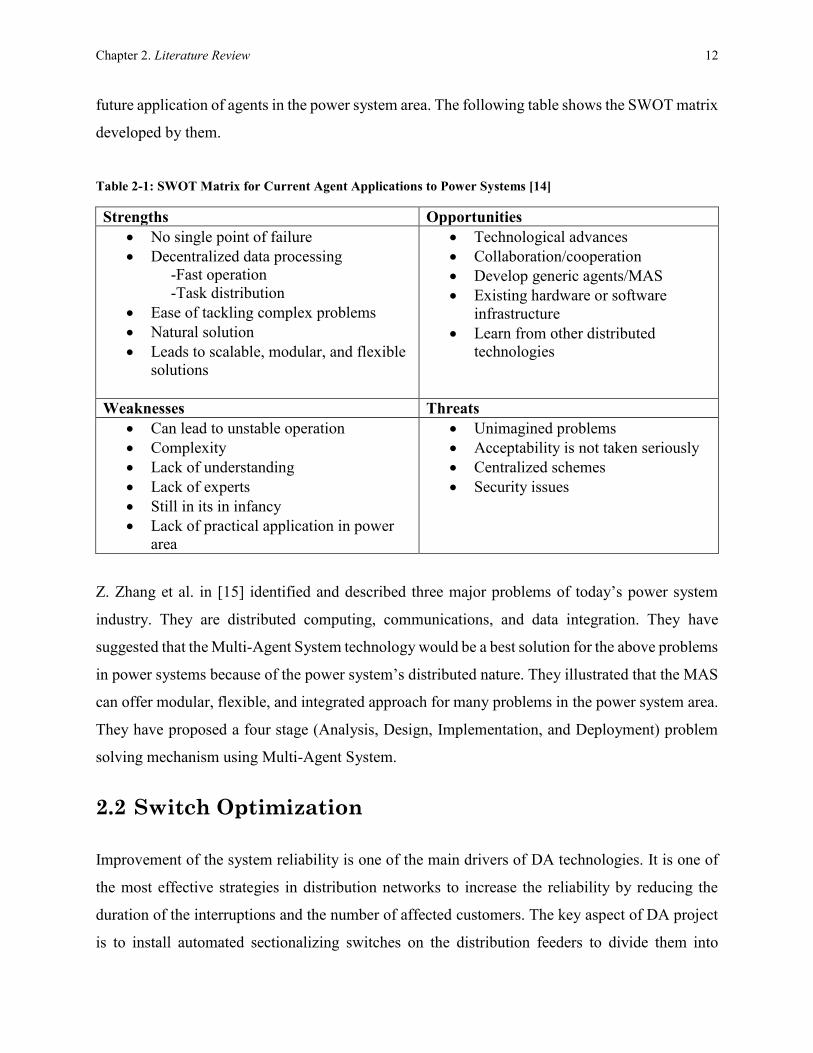
area. The authors in [14] have analyzed agent based technologies under the Strengths Weaknesses
Opportunities Threat (SWOT) framework. Based on the SWOT analysis they have envisaged the
Chapter 2. Literature Review 12
future application of agents in the power system area. The following table shows the SWOT matrix
developed by them.
Table 2-1: SWOT Matrix for Current Agent Applications to Power Systems [14]
Strengths Opportunities
No single point of failure
Decentralized data processing
-Fast operation
-Task distribution
Ease of tackling complex problems
Natural solution
Leads to scalable, modular, and flexible
solutions
Technological advances
Collaboration/cooperation
Develop generic agents/MAS
Existing hardware or software
infrastructure
Learn from other distributed
technologies
Weaknesses Threats
Can lead to unstable operation
Complexity
Lack of understanding
Lack of experts
Still in its in infancy
Lack of practical application in power
area
Unimagined problems
Acceptability is not taken seriously
Centralized schemes
Security issues
Z. Zhang et al. in [15] identified and described three major problems of today’s power system
industry. They are distributed computing, communications, and data integration. They have
suggested that the Multi-Agent System technology would be a best solution for the above problems
in power systems because of the power system’s distributed nature. They illustrated that the MAS
can offer modular, flexible, and integrated approach for many problems in the power system area.
They have proposed a four stage (Analysis, Design, Implementation, and Deployment) problem
solving mechanism using Multi-Agent System.
2.2 Switch Optimization
Improvement of the system reliability is one of the main drivers of DA technologies. It is one of
the most effective strategies in distribution networks to increase the reliability by reducing the
duration of the interruptions and the number of affected customers. The key aspect of DA project
is to install automated sectionalizing switches on the distribution feeders to divide them into

Chapter 2. Literature Review 13
multiple zones. The sectionalization of the feeder helps improving the reliability by isolating the
faulted zone, and serving the un-faulted zones by adjacent feeders. The first step in any DA
project’s economic feasibility is the determination of number and placement of sectionalizing
switches.
The problem of determining optimal number and placement switches has been studied by several
authors with different approaches. Many works in literature formulated the problem as an
optimization problem with objective functions such as reliability improvement and minimization
of investment cost of switches. The reliability improvement is modeled as minimization of
interruption costs. These methods are heavily reliant on the data pertaining to interruption costs
and switch investment costs. The main problem with such data is the fact that it is not openly
available, and even if it is available, seldom the data represent the present market conditions.
Therefore, implementation of switch optimization problem using the actual values of interruption
costs and investment costs might not always result in correct answer.
Authors in [16] proposed a Genetic Algorithm (GA) based approach to determine the best number
of switches and their placement. A binary representation model and reliability measure SAIDI
calculated from the annual non-supplied energy were used in the approach. Authors in [16] also
proposed a solution to optimally allocate switches, reclosers, and fuses. The device allocation
problem was modeled with non-linear integer programming and reliability index SAIFI was used
as the objective function.
A Simulated Annealing approach is proposed in [17] which considered the investment,
maintenance, and outage costs in a single global cost function to determine the optimal number
and location of switches. A decomposition approach is presented in [18] and the solution is
represented as a binary array of the possible locations for sectionalizing switches. The problem
complexity was reduced by using a polynomial-time partitioning algorithm to decompose the
problem into a set of convex independent sub-problems to be solved independently.
Authors in [19] proposed an immune algorithm to solve the problem of optimal allocation of
switches. The solution was to minimize the objective function which is sum of the customer

Chapter 2. Literature Review 14
interruption cost and the investment cost of installing switches. The immune algorithm based
solution was used to design the DA system for a real distribution system in Taiwan Power
Company. The work in [20] uses a reactive tabu search to find the optimal device allocation. The
objective function was a sum of estimated interruption costs.
Authors in [21] proposed the solution based on cost/worth approach and the best locations of
switches are determined by Simulated Annealing algorithm. A trade off analysis between
sectionalizing switch cost to the reliability worth was used in the solution. A Particle Swarm
optimization approach was proposed in [22] to determine the optimum number and locations of
two types of switches, sectionalizer and breakers, in radial distribution systems. Authors in [23]
proposed an Ant Colony optimization based method using fuzzy multi-objective formulation for
finding the number and location of sectionalizing switches in distribution networks including DG.
2.3 Fault Location and Isolation
Fault location in distribution systems is an important function for outage management and service
restoration. It directly impacts feeder reliability and quality of the electricity supply for the
customer. Fault location is a more challenging task in distribution systems than transmission
systems. This is due to the nature of the distribution systems such as heterogeneity of the lines,
presence of laterals, load taps, presence of distributed generation, and comparatively a lower
degree of instrumentation [24]. The methods aimed at transmission level usually use data from
Power Quality (PQ) monitors and protection devices. At distribution level, the data is usually more
limited with inadequate communication infrastructure.
The existing fault location methods in the literature can be mainly classified into three categories:
1. Impedance based methods
2. Wavelet based methods
3. Intelligent methods such as Artificial Neural Networks (ANNs), Expert Systems, and
MAS.

Chapter 2. Literature Review 15
Impedance based methods usually calculate the apparent impedance using the voltage and current
phasor measurements from field devices. The apparent impedance is used to estimate the potential
fault locations in the system based on specific algorithms. These methods can successfully locate
the faults for distribution systems that have fairly simple structures without many lateral taps. The
common drawback is that the fault location results in multiple fault location estimations due to
their reliance solely on measured voltage and current signals at the substation. A detailed review
of the existing impedance methods is presented in [25].
Recently some methods have been developed and adopted by utilities for fault location based on
the Impedance approach. In [26], an approach is introduced to compute apparent reactance by
using fundamental voltage and current phasors and estimated fault location based on the computed
reactance. At distribution level, the performance of this method suffers due to load effects. In [27],
Santoso et al. utilized load changes to identify the line sections where the fault may have occurred.
In [28], a current and impedance change method has been adopted to estimate the location of the
fault in the distribution system with distributed generation.
In [29] [12] the authors used the data from PQ monitors and compared the data with simulation
data for better fault location. In [30], Saha et al. adopts a similar approach and proposes to use the
data from the existing microprocessor relays. To overcome the line model dependency problem,
in [31] an ANN based estimator was proposed to estimate fault locations. In [32], after the
candidate sections are found, the feeder topologies and load current change were considered to
further rank candidate fault locations.
Some fault location methods have been developed that uses wavelet analysis of fault current
waveforms using Fourier Transform. These methods are less reliable because of variety of load
characteristics and fault causes in distribution systems. Authors in [33] introduced a wavelet based
method for the detection of High-Impedance Ground Faults (HIF) in distribution systems. The
ground faults are detected by the estimation of phase displacements between zero-sequence
voltage currents in the feeders. It is shown that the analysis of transients in zero-sequence currents
and voltages in wavelet domain leads to fast and reliable HIF detection and localization of the

Chapter 2. Literature Review 16
faulted feeder. The proposed algorithm remains stable for any network changes, and is independent
of the network neutral-point grounding mode.
Fault location methods based on intelligent systems such as neural networks and fuzzy logic are
proposed in [34], [35]. The major limitation of intelligent methods with learning is the fact that
they require retraining with huge amount of data sets subsequent to every change in system
topology. In [34], faulted area is detected by training an Adaptive Neuro-Fuzzy Inference System
(ANFIS) net with extracted features based on knowledge about protective device settings. In [35]
using the Learning Algorithm for Multivariable Data Analysis (LAMDA) classification technique,
multiple fault location estimation solution is obviated.
2.4 Service Restoration
The service restoration is a combinatorial problem since it involves many combinations of
switching operations to restore power to customers during emergencies. Presently, service
restoration problem is solved using various approaches such as Heuristics [36] , Expert Systems
[37], Meta-Heuristics [38, 39, 40], and Mathematical Programming [41] [42]. Some of the Meta-
Heuristic techniques like Genetic Algorithm (GA), Particle Swarm Optimization (PSO), Simulated
Annealing (SA), and Tabu Search (TS) have been used extensively for the restoration problem.
Artificial Neural Network (ANN), Dynamic Programming, and Ant Immune System - Ant Colony
Optimization (AIS-ACO) are also studied for restoration problem.
A key disadvantage of most of the techniques for service restoration problem mentioned above is
the fact that they all work in a centralized fashion to solve the problem. All of these techniques
require a powerful central computing facility with high communication requirements to haul huge
amounts of data with minimal latency. This dependency can lead to a single-point-of-failure
defeating the key purpose of DA systems to improve system reliability.

Chapter 2. Literature Review 17
2.4.1 Expert Systems and Heuristics
Expert Systems and Heuristic methods use some rule-based programming logic based on
operator’s knowledge and experience. This reduces the search space of the combinatorial
restoration problem and the solution is achieved in less time with minimal computational burden.
The main drawbacks of Heuristic methods are, optimal solution is not guaranteed, and the software
that handles the rule-set can become complex as the system size grows. Morelato and Monticelli
[36] have presented a Heuristic search approach for distribution system restoration which uses a
knowledge guided search strategy to reach the solution. Liu et al. in [37] designed an Expert
System algorithm for restoration and loss reduction of distribution systems. The authors
constructed a knowledge base which contains rules that implement a solution approach that system
operators can use for service restoration.
2.4.2 Mathematical Programming
The Mathematical Programming approach determines the target configuration for restoration often
by formulating the problem as a Mixed Integer Non-Linear Problem (MINLP). In the formulation
each switch status is denoted with a binary value “1” if the switch status is close and “0” if the
switch status is open. Other parameters such as voltage and thermal capacity are modeled as
continuous variables to specify the constraints for the optimization problem. The mathematical
programming can find optimal target reconfiguration, however, the main drawback of this
technique is computational intensity and it might not be a practical solution for large distribution
systems.
Nagata et al. in [43] proposed a two-stage algorithm which decomposes the restoration problem
into two sub-problems, one to maximize available power to the de-energized area, and two to
minimize the amount of unserved energy. The algorithm was tested on dc models which does not
take into account the reactive power as well as voltage variations. Authors in [42], presented a
Dynamic Programming approach with state reduction for service restoration in radial distribution
system. The timing and selection of feeders to be energized are represented as states in a Dynamic
Programming formulation. The proposed Dynamic Programming method reduces the number of

Chapter 2. Literature Review 18
states by grouping states that are close to each other and selecting the best state. S. Das et al. in
[41] presented a restoration methodology based on reinforcement learning for ship-board power
system. The proposed approach not only determines the optimal target configuration but also the
correct order in which the switches are to be changed.
2.4.3 Multi-Agent System technology
Multi-Agent System technology emerges as an application of distributed intelligence that deals
with concentrating the intelligence on a component level. MAS is a computational system in which
several agents cooperate and coordinate with each other to achieve organizational objectives in a
decentralized fashion [44]. This technology is superior to centralized schemes mentioned above as
even though a part of the system fails rest of the system still continues to work. MAS can be
considered as the platform of distributed processing, parallel operation, and autonomous solving.
Further, it can be much faster in solving discrete and nonlinear problems. Therefore, MAS as a
distributed restoration algorithm represents an interesting candidate for restoration and control of
the distribution system to realize the self-healing operation. In the past, several authors have
worked on MAS technology for solving service restoration problem in power systems.
J. M. Solanki et al. in [45] introduced a totally decentralized MAS solution for the service
restoration in distribution systems. The Multi-agent platform is developed in Java Agent
Development Framework (JADE) and the power system test case is developed in Virtual Test Bed
(VTB). In their work they proposed three new agents named Switch Agents (SAs), Load Agents
(LAs), and Generator Agents (GAs). The agents communicate only to their neighboring agents
and act locally, making the restoration scheme decentralized. The restoration algorithm has certain
objectives and constraints like, limit on generation, priority of loads, and transfer capacity of lines.
Nagata et al. in [46, 47] have proposed a Multi-agent architecture for power system restoration
problem. This architecture was fully decentralized one, in which the agents communicate and
negotiate only with their neighboring agents. In this work authors have used two types of agents
named Bus Agents (BAGs) and Facilitator Agent (FAG). BAG is a bus agent situated at each and
every bus in the network, whereas, FAG is a Facilitator Agent situated on top of all BAGs for the

Chapter 2. Literature Review 19
decision making purpose. BAGs communicate with their neighboring agents to find out the sub-
optimal target configurations, whereas, FAG acts as a manager for decision process. Knowledge
Query and Manipulation Language (KQML) is used as an agent communication language.
In [48], authors have proposed a more complicated four layered agent architecture for the bulk
power system restoration. A single Independent System Operator Agent (ISOAG) which controls
the timing of the simulation process forms the higher level in the agent architecture. The second
level consist several Local Area Management Agents (LAMs) for the local area management of
the restoration. Third level of architecture has several Load Facilitator Agents (LFAGs), Generator
Facilitator Agents (GFAGs), and Remote Facilitator Agents (RFAGs). These agents will facilitate
with the agents situated in the fourth layer of architecture, which include Load Agents (LAGs) and
Generator agents (GAGs). The authors have applied the proposed MAS to bulk power system and
the simulation results are very promising.
Authors in [49] have also contributed in the field of Multi-Agent System for bulk power system
restoration. The method employed in this work makes use of both centralized and decentralized
schemes to obtain the restoration solution. The agent architecture has two hierarchical agents
called, Management Agents (MGAGs) and agents representing practical power system
components (PCAGs). Each PCAG monitors several agents related to a subsystem named
Generator Agents (GAGs), Substation Agent (SAGs), and Load Agents (LAGs). One MGAG is
generated in charge of the subsystem and provides negotiations and communications between
PCAGs and with other subsystems.
Authors in [6] proposed a hybrid MAS solution for fault detection and service restoration problem.
The proposed approach in [6] reconfigures the system in a way to supply all the critical loads.
When there are multiple solutions available for reconfiguration, the one with good voltage profile
and less power loss is selected as the solution. The proposed algorithm makes use of shunt
compensation and priority based load shedding in order to control the voltage across the network.
Authors in [50] have used artificial immune system algorithm for the fault restoration problem. In
[51] the author demonstrated a practical implementation of MAS for FLIR in which agents are
implemented in microprocessors and the distribution system is simulated using a power systems
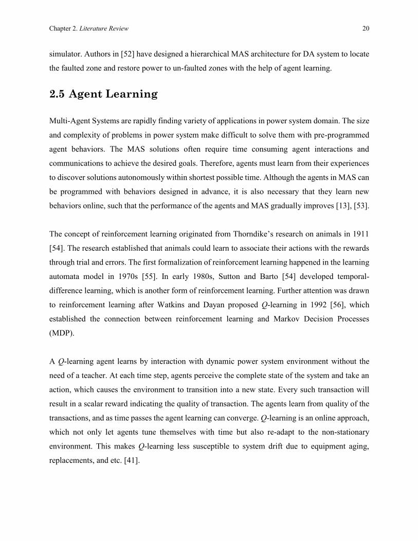
Chapter 2. Literature Review 20
simulator. Authors in [52] have designed a hierarchical MAS architecture for DA system to locate
the faulted zone and restore power to un-faulted zones with the help of agent learning.
2.5 Agent Learning
Multi-Agent Systems are rapidly finding variety of applications in power system domain. The size
and complexity of problems in power system make difficult to solve them with pre-programmed
agent behaviors. The MAS solutions often require time consuming agent interactions and
communications to achieve the desired goals. Therefore, agents must learn from their experiences
to discover solutions autonomously within shortest possible time. Although the agents in MAS can
be programmed with behaviors designed in advance, it is also necessary that they learn new
behaviors online, such that the performance of the agents and MAS gradually improves [13], [53].
The concept of reinforcement learning originated from Thorndike’s research on animals in 1911
[54]. The research established that animals could learn to associate their actions with the rewards
through trial and errors. The first formalization of reinforcement learning happened in the learning
automata model in 1970s [55]. In early 1980s, Sutton and Barto [54] developed temporal-
difference learning, which is another form of reinforcement learning. Further attention was drawn
to reinforcement learning after Watkins and Dayan proposed Q-learning in 1992 [56], which
established the connection between reinforcement learning and Markov Decision Processes
(MDP).
A Q-learning agent learns by interaction with dynamic power system environment without the
need of a teacher. At each time step, agents perceive the complete state of the system and take an
action, which causes the environment to transition into a new state. Every such transaction will
result in a scalar reward indicating the quality of transaction. The agents learn from quality of the
transactions, and as time passes the agent learning can converge. Q-learning is an online approach,
which not only let agents tune themselves with time but also re-adapt to the non-stationary
environment. This makes Q-learning less susceptible to system drift due to equipment aging,
replacements, and etc. [41].

Chapter 2. Literature Review 21
In this dissertation, a MAS concept for self-healing power distribution grids with agent learning
capability is proposed. The main note-worthy contribution of this research is the modified Q-
Learning approach to solve service restoration problem in power distribution systems with
distributed energy resources. The learning methodology is used to teach agents to use their
experiences and update their knowledge as the system is operational. The Q-Learning technique
introduced in this dissertation uses Q-matrix and switch combination matrix as the repositories for
all the information learned through previous restoration experiences. Agents can utilize the
learning for service restoration instead of performing time consuming optimization, if there is
sufficient learning from restoration experiences.
Q-learning has been extensively used to solve the strategy control and learning problems of
autonomous agents. Sanjoy Das et al. in [41] used Q-Learning for dynamic reconfiguration of
shipboard power systems. The problem of service restoration is formulated as an optimization
problem with an objective to maximize the weighted sum of the power delivered to the loads. The
prosed approach is a dynamic technique that produces not only the final reconfiguration, but also
the correct order in which the switches are to be changed. In [57] Q-Learning is used for power
system restoration following catastrophic disturbances involving loss of generators. The proposed
Q-learning restorative framework supports agents to make accurate decision in a timely manner to
restore the system without requiring a global reward signal. Jung et al. in [58] presented a Multi-
agent framework to avoid catastrophic failures of a power system by introducing an adaptive agent
learning method for load shedding based on Temporal Difference (TD) method, which is one of
the forms of Reinforcement Learning (RL).
2.6 Existing FLIR Systems
Until the 1990s, technological breakthroughs in the automation of electric distribution systems
were slow to materialize. Early SCADA systems promised to improve reliability. But many of the
early systems were little more than an extension of SCADA beyond the substation fence. With
their relatively low computational and communication capabilities, these early systems required a
high degree of human intervention and offered little in the way of true automation. As a result,
expectations were not always met, leading to the termination or scaling back of many projects.

Chapter 2. Literature Review 22
Nevertheless, many lessons were learned and technology has advanced, especially through the
1990s and to the present. More advanced automation applications have been developed that are far
more practical and manageable for utilities to implement. Some tools for feeder automation have
been available for many years. Below we presented the S&C Electric Company product
(IntelliTEAM-SG) which is a patented and commercialized product and compare it to the proposed
FLIR system presented in this dissertation [4, 59].
2.6.1 IntelliTeam SG
In 2003, the IntelliTEAM Automatic Restoration System was introduced by S&C Electric
Company. IntelliTEAM II is a patented automatic power restoration system that uses distributed
intelligence and peer-to-peer communication to switch and isolate the faulted line section and
restore power to un-faulted line sections.
IntelliTEAM utilizes ties to multiple circuits, enabling a wide variety of circuit configurations to
maximize the restoration potential. Distributed intelligence prevents line overloads. IntelliTEAM
can automate parts of a circuit in need of attention or an entire distribution system consisting of
open-loop feeders with multiple tie points to other feeders. It can be used both tactically and
strategically, based on the reliability problems the utility needs to solve.
2.6.2 IntelliTeam Working Principle
IntelliTEAM dynamically tracks system conditions on overhead and underground distribution
systems and provides fully automatic fault isolation and service restoration. “Team" and “Coach"
metaphors help to describe IntelliTEAM operation. Each team is defined as a line segment
bounded by two to eight automated switches, each of which can represent a different power source.
Each team has a software coach. If an outage or line fault occurs, local control logic determines if
a switch should open. The coach of each affected team then uses real-time data, including voltage
and current data gathered prior to the system event to develop a restoration strategy for un-faulted
sections. The coaches of adjacent teams then work together through shared controls to implement
strategies that will maximize restoration of the circuit within the prioritization rules defined by the
user.

Chapter 2. Literature Review 23
Breakers and reclosers can also be incorporated as team members with the addition of a module
that interfaces to the electronic relay or control that operates the breaker or recloser. Figure 2-1
illustrates the team concept. The coach distributes data and coordinates the operation of automated
switches, reclosers, and breakers. Coach travels to each team member within a prescribed time
period. Coaches are responsible for restoration decision makings and they move to each switch
that has the capability for restoration and ask the neighboring team coach to move to the same
switch to make restoration decisions. When a coach moves to a team member to investigate the
restoration possibility, it searches for the neighboring coach from the adjacent teams.
In the event of a loss of communication, service restoration may be inhibited, but an automated
switch, recloser, or breaker can still isolate a fault based on local fault detection and isolation
software logic.
Figure 2-1: An Example of IntelliTEAM Implementation
At the beginning of a fault or outage event, any team member detecting the event will communicate
to all the other team members and the coach, reporting the time, type of event, report identification,

Chapter 2. Literature Review 24
and so on. The coach also monitors the status of each device, ensuring that all are in the right open
or closed position to allow progress to the next restoration step.
In order to close a switch, the coaches of adjacent teams must grant permission based on circuit
conditions, location of fault, and an evaluation of loading conditions. When all appropriate
conditions are met, the switch can be closed to restore service to a feeder segment. This process is
repeated for each segment in turn. As switches close, the IntelliTEAM system updates available
capacity on the feeders used to restore service, ensuring maximum service restoration even at
maximum peak load.
Following a reconfiguration event, and subsequent repair and restoration of the faulted line section,
team members can return to their normal state. Once the “return to normal" is initiated, the coaches
begin the process of returning each team to its normal configuration. The return-to-normal process
begins at the team closest to the normal source and works outward, using either an open or closed
transition approach as defined by the user.
To support the distributed control architecture of IntelliTEAM, a peer-to-peer wide-area
communication network is essential. There are only a few commercially available wide-area
communication systems that readily support such a network. Typically, communication for the
IntelliTEAM system is provided by 900-MHz UtiliNet spread- spectrum radios. The UtiliNet radio
system transports data using a connectionless mesh architecture. This architecture allows each
radio in the network to act as both a repeater radio and a data transceiver for an automated switch.
The radio network is highly scalable and obviates the need to invest in the tall master radio towers
prevalent in point-to multi point radio networks.
Fiber-optic networks have also been utilized for high speed peer-to-peer communication, typically
in underground applications where fiber is installed along with the underground cable
infrastructure.

Chapter 2. Literature Review 25
2.6.3 FLIR & IntelliTeam
In IntelliTEAM the local control logic determines if a switch should open after a loss of voltage,
and/or fault current event. A team member would open to isolate the fault after sensing the fault
currents and two times loss of voltage (because of recloser operations). Also, if a switch does not
sense the fault current it opens after two times loss of voltage. The fault location can be determined
based on the location of switches that sensed the fault current. This FLI method has the following
disadvantages:
It does not support the DG penetration: In case there are DG's in the power system and two
way power ow exists, proposed FLI system might not be able to locate the fault.
It requires threshold settings for fault currents which is challenging and should be modified
after any change in the system configuration.
For restoration, the coach of each affected team uses the real-time data, plus voltage and current
data gathered prior to the system event, to develop a restoration strategy for un-faulted sections.
The coaches work together to implement strategies that will maximize restoration within the
prioritization rules defined by the user. A coach moves from the switch to switch based on the
predefined source priorities and checks the restoration possibility through that switch and by
negotiating with the neighboring coaches.

26
Chapter 3
Multi-Agent Systems
Agent based technologies have been the subject of extensive research and investigation for several
years, but it is recently that MAS have been seen significant degree of exploitation in commercial
applications. Multi-Agent Systems have been used in vivid applications ranging from small
systems to most intrinsic systems. Some of the fields where these Multi-Agent Systems have been
fruitfully employed include process control, system diagnostics, manufacturing, transportation
logistics, and network management [44].
Before understanding the Multi-Agent Systems, one has to understand the concepts behind the
single agent. Many people have defined the word “agent” in their own ways since the starting of
agent technologies. Out of many definitions available a couple of relevant definitions are given
below,
“An agent is an autonomous computational entity such as a software program that can be viewed
as perceiving its environment through sensors and acting upon this environment through its
effectors” – Weiss [13].
“An agent is a computer system that is situated in some environment, and that is capable of
autonomous action in this environment in order to meet its design objectives” – Wooldridge and
Jennings [60].

Chapter 3. Multi-Agent Systems 27
The above two definitions are much suitable for this dissertation work. Multi-Agent Systems
received greater attention in the recent past in many intelligent and distributed systems to model
the theories of interactivity in human societies. Humans interact in various ways and at different
levels. For an instance, humans observe and model one another, they request and provide
information, they negotiate and discuss, they develop shared views of their environment, they
detect and resolve conflicts, and they form organizational structures such as teams, committees,
and economies.
In this dissertation the term agent means, a software entity which perceives its environmental
changes and acts on it diligently to achieve its organizational objectives. A Multi-Agent System
means the collection of such agents which communicate and coordinate to solve a particular
problem according to their objectives. The Multi-Agent System approach for electric distribution
system is shown in Figure 3-1,
Electric Distribution System (EDS)
Agent
SenseAct
Figure 3-1: Multi-Agent System for Electric Distribution System
The main problem facing by an agent is deciding which of its actions it should perform in order to
best satisfy its organizational objectives. The type of decision selected always depends upon the

Chapter 3. Multi-Agent Systems 28
type of environment. Russell and Norvig [61] proposed following classification of environment
properties,
Accessible vs Inaccessible.
An accessible environment is one in which all the states of the environment are easily
accessible. But, most of today’s complex networks, such as every day physical world and
Internet, are inaccessible.
Deterministic vs Non-deterministic
In deterministic environment the actions will have certain effects on the environment. In
non-deterministic environments it is difficult to anticipate the effects of particular action
on the environment. Non-deterministic environments will have greater difficulty in
designing.
Episodic vs Non-episodic
In an episodic environment, the performance of an agent is dependent on a number of
episodes, such as mail sorting system.
Static vs Dynamic
A static environment is one that can be assumed to be unchanged except for the actions by
agent. In contrast to the static environment the real world systems are dynamic systems
which change from time to time, hence, difficult to control.
Discrete vs Continuous
An environment is said to be discrete, if it has discrete number of actions and percepts in
it. The best example for a discrete environment is the chess game and for a continuous
environment is car driving.
Comparing the agents to the present world computer systems, every action a computer performs
is anticipated, planned for, and coded by a programmer. When a computer encounters a new sort
of problem, which is not anticipated, then the system will crash. This is because the computer
systems do not have intelligence embedded in it. Unlike the computer systems the agents are
intelligent enough to take up the flexible autonomous actions to satisfy their objectives [60]. Here
the flexibility means three things,

Chapter 3. Multi-Agent Systems 29
Reactivity:
Agents are able to perceive their environment, and respond in a timely fashion to changes
that occur in it, in order to satisfy their objectives.
Pro-activeness:
Intelligent agents are able to exhibit goal oriented behavior by taking the initiative in order
to satisfy their objectives.
Social-ability:
Intelligent agents are able to communicate and cooperate with other agents available in
Multi-Agent Systems in order to satisfy their objectives.
Out of the above three characteristics the social-ability is the more complex one. In real world
daily millions of computers exchange the information with both humans and other computers. But,
the ability to exchange the bit stream is not really the social ability. Consider the human world
where humans achieve their goals by negotiation and cooperation [13]. The same way intelligent
agents cooperate and negotiate with each other to achieve the common goal of the Multi-Agent
System. The communication between the agents in MAS has certain standards defined by
Foundation for Intelligent Physical Agents (FIPA).
There is always been a great amount confusion between agents, objects, and expert systems. The
main distinctions between traditional view of an object and an agent is listed below [13],
Agent embody a strong notion of autonomy than objects, they decide on themselves
whether or not to perform an action on request from other agents.
Agents are capable of flexible (reactive, pro-active, social) behavior. Where, objects have
no such behaviors.
A MAS is inherently multi-threaded where each agent has at least one thread of control.
Expert Systems are the most important Artificial Intelligence (AI) technology of 1980s [62]. An
Expert System is one that is capable of solving problems or giving advice in some knowledge rich
domain [13] [63]. The main difference between Expert Systems and Agent technologies is that, an
Expert System cannot sense its environment directly. Instead, it needs a middle man to input the

Chapter 3. Multi-Agent Systems 30
data. In the same way an Expert System cannot act directly on its environment. It just gives certain
instructions to the operator.
3.1 Agent Communication
It has been seen in the earlier section that agents communicate to coordinate and negotiate on
particular tasks to achieve its organizational objectives. The communication ability of agents is
part perception (the receiving of messages) and part action (the sending of messages). There are
generally two message types in agent communication, Assertion and Queries. Every agent whether
active or passive, must have the capability to accept the information. In order to assume a passive
role in a dialogue, an agent must be able to 1) accept a query from an external source and 2) send
a reply to the source by making an assertion. In order to assume an active role in a dialogue, an
agent must have the capability to send queries and make assertions [13].
Communication protocols are very important in any communication systems. The Multi-agent
communication is specified by a data structure with the following five fields,
Sender.
Receiver(s).
Language in protocol.
Encoding and Decoding functions.
Action to be taken by the receiver(s).
Speech Act Theory helps in defining the message send by sender. So, the receiver has no doubts
regarding the received message [64]. In order to understand communication messages precisely,
all the agents in MAS has to follow the same ontology. Two agents following the same ontology
means, those two agents know the meaning of messages during the communication. Hence,
ontology results in perfect operation of communication. In technical terms the name ontology is
defined as follows,

Chapter 3. Multi-Agent Systems 31
“Ontology is a formal definition of a body of knowledge. The most typical type of ontology used
in building agents involves a structural component. Essentially a taxonomy of class and subclass
relations coupled with definitions of the relationships between these things” – Jim Hendler [13]
The most common languages followed for the agent communication are,
Agent Communication Language (ACL)
Knowledge Query and Manipulation Language (KQML)
3.1.1 FIPA-ACL
Foundation for Intelligent Physical Agents (FIPA) is an IEEE Computer Society Standards
organization that promotes agent-based technology and the interoperability of its standards with
other technologies. FIPA was originally formed as a Swiss based organization in 1996 to produce
software standards for heterogeneous and interacting agents and agent based systems [65].
FIPA has developed a certain number of standards for heterogeneous agent communications. FIPA
Agent Communication specifications deal with Agent Communication Language messages,
message exchange interaction protocols, speech act theory based communicative acts, and content
language representations.
Agent Communication Language developed by FIPA is based on speech act theory. Here the
messages are actions or communicative acts, as they are intended to perform some action by virtue
of being sent. The FIPA ACL specifications consist of a set of message types and the description
of their pragmatics, which is the effect on the mental attitudes of sender and receiver agents. A
sample FIPA ACL message is shown below,
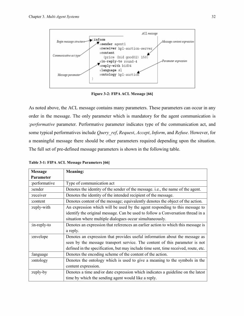
Chapter 3. Multi-Agent Systems 32
Figure 3-2: FIPA ACL Message [66]
As noted above, the ACL message contains many parameters. These parameters can occur in any
order in the message. The only parameter which is mandatory for the agent communication is
:performative parameter. Performative parameter indicates type of the communication act, and
some typical performatives include Query_ref, Request, Accept, Inform, and Refuse. However, for
a meaningful message there should be other parameters required depending upon the situation.
The full set of pre-defined message parameters is shown in the following table.
Table 3-1: FIPA ACL Message Parameters [66]
Message
Parameter
Meaning:
:performative Type of communication act
:sender Denotes the identity of the sender of the message. i.e., the name of the agent.
:receiver Denotes the identity of the intended recipient of the message.
:content Denotes content of the message; equivalently denotes the object of the action.
:reply-with An expression which will be used by the agent responding to this message to
identify the original message. Can be used to follow a Conversation thread in a
situation where multiple dialogues occur simultaneously.
:in-reply-to Denotes an expression that references an earlier action to which this message is
a reply.
:envelope Denotes an expression that provides useful information about the message as
seen by the message transport service. The content of this parameter is not
defined in the specification, but may include time sent, time received, route, etc.
:language Denotes the encoding scheme of the content of the action.
:ontology Denotes the ontology which is used to give a meaning to the symbols in the
content expression.
:reply-by Denotes a time and/or date expression which indicates a guideline on the latest
time by which the sending agent would like a reply.

Chapter 3. Multi-Agent Systems 33
:protocol Introduces an identifier which denotes the protocol which the sending agent is
employing. The protocol serves to give additional context for the interpretation
of the message.
:conversation-id Introduces an expression which is used to identify an ongoing sequence of
communicative acts which together form a conversation. A Conversation may
be used by an agent to manage its communication strategies and activities.
The Java Agent Development Environment (JADE) developed by Telecom-Italia makes use of
ACL protocol for agent communication.
3.1.2 KQML
Knowledge Query and Manipulation Language (KQML) is older than the FIPA ACL language.
KQML is a protocol for exchanging information and knowledge. The advantage of KQML
language is that, all information for understanding the content of the message is included in the
message pattern itself [13]. The basic protocol for the KQML language is defined by the following
structure,
(KQML-performative
: sender <word>
: receiver <word>
: language <word>
: ontology <word>
: content <expression>
…)
The KQML protocol for communications between agents and application program is illustrated in
Figure 3-3,

Chapter 3. Multi-Agent Systems 34
Figure 3-3: KQML Communication Protocol [13]
Most of today’s agent based platforms have migrated to FIPA ACL language for the agent
communications.

35
Chapter 4
MAS FLIR System Design
4.1 Proposed MAS Architecture
The proposed hybrid MAS has five types of agents namely Substation Agent (SA), Feeder Agent
(FA), SSW Agent (SSA), TSW Agent (TSA), and PCC Agent (PA) distributed in three hierarchical
layers as shown in Figure 4-1. As the name indicates these agents are situated at the respective
hardware points in the real field. The total number of agents for a self-healing FLIR system
depends on total number of substations, feeder reclosers/breakers, SSW, TSW, and PCC switches
present in the targeted distribution system.
Each layer has a set of agents that can communicate with other agents in the same layer and with
the agents that they are associated in the downward layer. FA can communicate with its
neighboring FAs in the same layer, and with its children SSAs, TSAs, and PAs in the downward
layer. This makes the MAS architecture hierarchical. However, the supervisory agents, FA and
SA, also exploit peer to peer communications with the lower level switch agents to reduce number
of communications to speed up the FLIR processes. The decision making happens at the
supervisory level, at the FA or SA level, as these agents have the complete view of the system to
achieve the optimal solution.
Each agent knows limited local information and if it needs information outside its boundaries it
communicates with respective agents to gather that information. For e.g., if a SSA wants to know
about the available feed capacity of a particular TSA, then it communicates with that respective

Chapter 4. MAS FLIR System Design 36
TSA to gather the required information. This arrangement makes the MAS architecture to be
modular and decentralized.
PCC Agent
FA Feeder Agent SSA SSW Agent TSA TSW Agent
PA
FAn
FA3
FA1
FA2
SSAn
SSA3
SSA1
SSA2
Communication
Layer-2
Layer-3
SAn
SA3
SA1
SA2
Layer-1
SASubstation
Agent
TSAn
TSA3
TSA1
TSA2 PAn
PA3
PA1
PA2
Figure 4-1: Proposed Hybrid MAS Architecture
4.1.1 Agents
The agents are intelligent units that have problem solving capabilities and can communicate,
resolve, coordinate with other agents to achieve specific FLIR goals. The agents are
accommodated in ruggedized computers with required computing power and memory which are
powered by Uninterrupted Power Supply (UPS). A typical agent platform has the operating system

Chapter 4. MAS FLIR System Design 37
and needed software for communications and protocol conversions. Agent platforms support the
following associated functions:
Execution of advanced FLIR algorithms housed in the agents
Collection of data in the distribution field and at substations to support modeling, agent
learning, and system operations
Interpretation of data encoded using various protocols including DNP 3.0, Modbus, and
IEC-61850
Translation of data from one message protocol to another to support integration of
components utilizing multiple formats and protocols
Storage of data in the field supporting archival and efficient utilization of communications
throughout
Remote asset monitoring
Operating system supporting execution of functional source code including C, JAVA, C++,
and .NET framework applications
Different types of agents involved in the proposed architecture are explained in detailed below.
The actual work that an agent does is carried out in behaviors with different communication acts
mentioned as performatives following the ACL format. Table 4-1 provides an exhaustive set of
individual agent knowledge, capabilities, and behaviors.
4.1.1.1 Substation Agent (SA)
The SAs at the top layer act as back-up agents for decision making if any of the FA fails to perform
its responsibilities. Also, these agents perform supervisory monitoring of the FAs. The SAs mimic
FAs in terms of functionalities and capabilities.
4.1.1.2 Feeder Agent (FA)
The FAs and SAs are the main decision making agents, as these agents will have overall system
view to optimize the FLIR processes. FA is responsible for monitoring the feeder breaker or

Chapter 4. MAS FLIR System Design 38
recloser status and the measured data (current, voltage, real and reactive powers) at its location.
FA houses agent learning module which learns from past FLIR actions in a continuous fashion to
help with future service restoration events. FA also houses the FLI scheme to locate and isolate
the fault that can occur in its own zone. As soon as FA receives Fault Isolation message from one
of its SSAs, it starts service restoration of un-faulted zones either by utilizing the agent learning or
by mathematical optimization that involves TRA and ZPA algorithms. It can communicate with
all the downstream SSAs, TSAs, and PAs in a peer to peer manner to execute the service
restoration activities. A detailed functionality diagram is shown in Figure 4-2.
4.1.1.3 Sectionalizing Switch Agent (SSA)
SSA is responsible for monitoring the SSW status and the measured data (current, voltage, real
and reactive powers) at its location. SSA houses FLI scheme to locate and isolate the fault that can
occur in its own zone. It can communicate with the neighboring SSAs, and TSAs, and PAs present
in its zone to compute net pre-fault loading and zone current information. A detailed functionality
diagram is shown in Figure 4-2.
4.1.1.4 Tie Switch Agent (TSA)
TSA is responsible for monitoring the TSW status and the measured data (current, voltage, real
and reactive powers) at its location. TSA keeps the available feed capacity information. It can
communicate with its parent SSA and FA to help with service restoration activities. A detailed
functionality diagram is shown in Figure 4-2.
4.1.1.5 PCC Agent (PA)
PA is responsible for monitoring the PCC Switch status and the measured data (current, voltage,
real and reactive powers) at its location. It can communicate with its parent SSA and FA to help
with FLI and service restoration activities. A detailed functionality diagram is shown in Figure
4-2.

Chapter 4. MAS FLIR System Design 39
Feeder Agent (FA)
Feeder Recloser
Learning Module
FLIR
Algorithms
CT/PTs
PQ Meter
Communication
Protocol
Converter
Learning
Database
Policy
Selection
Q-updateReward
Calculator
State
Evaluation
Sectionalizing
Switch Agent (SSA)
Sectionalizing Switch
FLI Algorithms
CT/PTs
PQ Meter
Communication
Protocol
Converter Tie Switch
Agent (TA)
Tie Switch
TSW
Information
CT/PTs
PQ Meter
Communication
Protocol
Converter
Network
Power flow
PCC Agent (PA)
PCC Switch
PCC
Information
CT/PTs
PQ Meter
Communication
Protocol
Converter
SSW
Information
Recloser
Information
Figure 4-2: Agent Functionality Diagram
Table 4-1: Agent Knowledge/Capabilities and Behaviors
Agent Knowledge/Capabilities Behaviors
SA
1. Knowledge of its children FAs and their
children SSAs, TSAs, and PAs
2. Knowledge of neighboring SAs
3. Substation transformer nameplate capacity
(kVA)
4. System network model
5. Maintains NEZ_A and NEZ_B lists of its
children FA
6. Computing power to run power flows, FLI,
service restoration, and agent learning
processes
7. Agent learning database
Behaviors in normal mode
1. QUERY_REF behavior to request its children FA
information.
2. QUERY_REF behavior to check its children FA if it is
alive and performing FLIR tasks.
Behaviors in contingency mode when FA fails
1. QUERY_REF behavior to request net pre-fault
loading from its children FA’s children SSA.
2. QUERY_REF behavior to request its children FA’s
children TSA information.
3. REQUEST behavior to command its children FA’s
children SSA, TSA, or PA to open/close the respective
switch.
FA
1. Knowledge of its parent SA
2. Knowledge of its neighboring FAs
3. Knowledge of its children SSAs, TSAs,
and PAs
4. Knowledge of local measurements voltage
(V), current (A), real power (kW), and
reactive power (kvar)
5. Knowledge of feeder recloser or breaker
status (open/close)
1. INFORM behavior to send information to its parent
SA.
2. QUERY_REF behavior to request its neighboring FA
information.
3. INFORM behavior to send requested information to
its neighboring FA.
4. QUERY_REF behavior to request net pre-fault
loading from its children SSA.

Chapter 4. MAS FLIR System Design 40
6. Maintains NEZ_A and NEZ_B lists
7. System network model
8. Computing power to run power flows, FLI,
service restoration, and agent learning
processes
9. Agent learning database
5. QUERY_REF behavior to request its children SSAs to
initiate FLI process.
6. QUERY_REF behavior to request its children TSA
information.
7. REQUEST behavior to command its children SSA,
TSA, or PA to open/close the respective switch.
SSA
1. Knowledge of its parent FA and SA
2. Knowledge of its neighboring SSAs
3. Knowledge of TSAs, and PAs in its zone
4. Knowledge of local measurements voltage
(V), current (A), real power (kW), and
reactive power (kvar)
5. Knowledge of SSW status (open/close)
6. Computing power to run FLI processes
1. INFORM behavior to send net pre-fault loading
information to its parent FA or SA.
2. INFORM behavior to send FLI information to its
parent FA or SA.
3. ACCEPT behavior to perform requested switching
action by its parent FA or SA.
4. QUERY_REF behavior to request its pre-fault
measurements from TSAs and PAs in its zone.
5. QUERY_REF behavior to request pre-fault
measurements from its neighboring SSAs.
6. INFORM behavior to send requested information to
its neighboring SSA.
7. REQUEST behavior to command its neighboring SSA
to open/close the respective switch.
8. ACCEPT behavior to perform requested switching
action by its neighboring SSA.
TSA
1. Knowledge of its parent FA, SA, and SSA
2. Knowledge of its neighboring TSAs and
PAs
3. Knowledge of local measurements voltage
(V), current (A), real power (kW), and
reactive power (kvar)
4. Knowledge of TSW type and Available
Feed Capacity (AFC)
5. Knowledge of TSW status (open/close)
1. INFORM behavior to send pre-fault measurements
information to its parent SSA.
2. ACCEPT behavior to perform requested switching
action by its parent FA or SA.
PA
1. Knowledge of its parent FA, SA, and SSA
2. Knowledge of its neighboring TSAs and
PAs
3. Knowledge of local measurements voltage
(V), current (A), real power (kW), and
reactive power (kvar)
4. Knowledge of DG type (synchronous
generator, induction generator, or inverter
based DG)
5. Knowledge of facility type (individual DG,
or microgrid)
6. Knowledge of PCC switch status
(open/close)
1. INFORM behavior to send pre-fault measurements
information to its parent SSA.
2. ACCEPT behavior to perform requested switching
action by its parent FA or SA.

Chapter 4. MAS FLIR System Design 41
4.2 WVSC MAS Design
Figure 4-3 shows the WVSC distribution system, which is used to demonstrate the proposed MAS
FLIR solution with all agent placements. The targeted system for DA involves two substations,
WestRun and Pierpont substations. The WestRun substation has six outgoing feeders and each
feeder is protected by a recloser. The FAs are placed right at these recloser locations. The WR#3
and WR#4 feeders are strategically divided into several zones by SSWs and these zones are
connected to adjacent feeders through a set of TSWs. The SSAs and TSAs are placed at these
switch locations. In order to demonstrate the DG and microgrid elements of the proposed FLIR
solution a few fictitious DG and microgrid points are introduced in WR#3 feeder. The PAs are
placed right at the PCC switches of these DG and microgrid resources.
SSA1
SSA3
SSA5
TSA2
PA3
WestRun Substation
138 kV/12.5 kV
FA3
TSA4
TSA8
TSA7 TSA6
Z1
PA0
PA1
PA5
SG1
PV1
IG1
Z0
Z2
Z3Closed TSW/SSW
Open TSW/SSW
Closed PCC Switch
Open PCC Switch
SG2
PA11
Microgrid-1
PA22
Microgrid-2
SA1
FA4
TSA12
TSA15
SSA14
SSA10
SSA11
TSA9
FA5FA7FA1
Substation
Transformer
33.6 MVA
Pierpont Substation
138 kV/12.5 kV
Closed Recloser
Open Recloser
FA8
Substation
Transformer
33.6 MVA
TSA13 FA5p FA6
SA2
SG11
L11
SG22
L22
Z1
Z2
Z3
Figure 4-3: Agent Placement for WVSC Distribution System

Chapter 4. MAS FLIR System Design 42
4.3 Agent State Transition
Agents in the proposed MAS framework transition from one state to another as shown in the state
transition diagram in Figure 4-4. Agent can be in one of the following states at any given point of
time. The supervisory agents SA and FA make sure that all the agents in the MAS update their
state according to the system conditions. It is quite essential for agents to maintain these states as
it helps proper coordination among the agents to achieve the organizational goals of FLIR as a
single team.
Figure 4-4: Agent State Transition
Normal State: Agents stay in this state when the system they are connected to is operating
normally without any faults or contingencies. Agents spend most of their time in this state
and continuously monitor/record the data, and update the learning database if they have the
learning ability.
Fault State: Agents transition to this state when there is a permanent fault in the electric
distribution system.
Fault Location and Isolation State: Agents transition to this state when the fault location
and isolation process takes place right after the feeder recloser/CB locks-out.
Normal State
Fault State
Fault Location
& Isolation
State
Service Restoration State
Fault Repair State
Return to Normal
State

Chapter 4. MAS FLIR System Design 43
Service Restoration State: Agents transition to this state when the service restoration
process takes place soon after fault has been isolated.
Fault Repair State: Agents transition to this state when the fault is being repaired.
Return to Normal State: Agents transition to this state when the fault is fixed and
distribution operator wants to bring back the system to the normal state.
4.4 Proposed FLIR Process Flow
Figure 4-5 shows the process flow diagram of the proposed FLIR solution. As soon as a permanent
fault occurs on the electric distribution system the whole system transitions into the fault state, and
the feeder protection system operates to clear the fault. The permanent lock-out of the feeder
recloser/CB initiates the MAS to transition into the FLI state where all the zones on the faulty
feeder would isolate in preparation for service restoration. The SSAs of the faulty feeder employ
the “Fault Detection Algorithm” and with the help of coordinated agent communications the
faulted zone is identified and isolated. This triggers service restoration state, where the fault-free
zones that have no power are restored either from a potential solution from the “Agent Learning
Database” or by performing a restoration optimization.
The agents involved in the FLIR MAS are capable of perceiving the system conditions and learn
in a continuous fashion. Each time a successful FLIR action is taken by MAS the “Agent Learning
Database” would be updated with the MAS action and pre and post system state. If there is no
feasible solution exist in the “Agent Learning Database”, the concerned FA or SA performs
restoration optimization using “Tie-Switch Ranking Algorithm” and “Zone Priority Algorithm” to
find out the best possible restoration plan. The main objective of the restoration optimization is to
restore as many fault-free zones as possible using all the available Tie-switch options. The
optimization also accounts for existing DG units and microgrids. Once the solution is discovered,
the FA/SA initiates commands to its downstream agents to implement the restoration plan. The
next stage is where the utility personnel repair the faulty portion or equipment of the system. Once
the fault is cleared, the distribution operator initiates MAS return to normal procedure. The MAS
follows the proposed procedure to bring back the system to normal state.
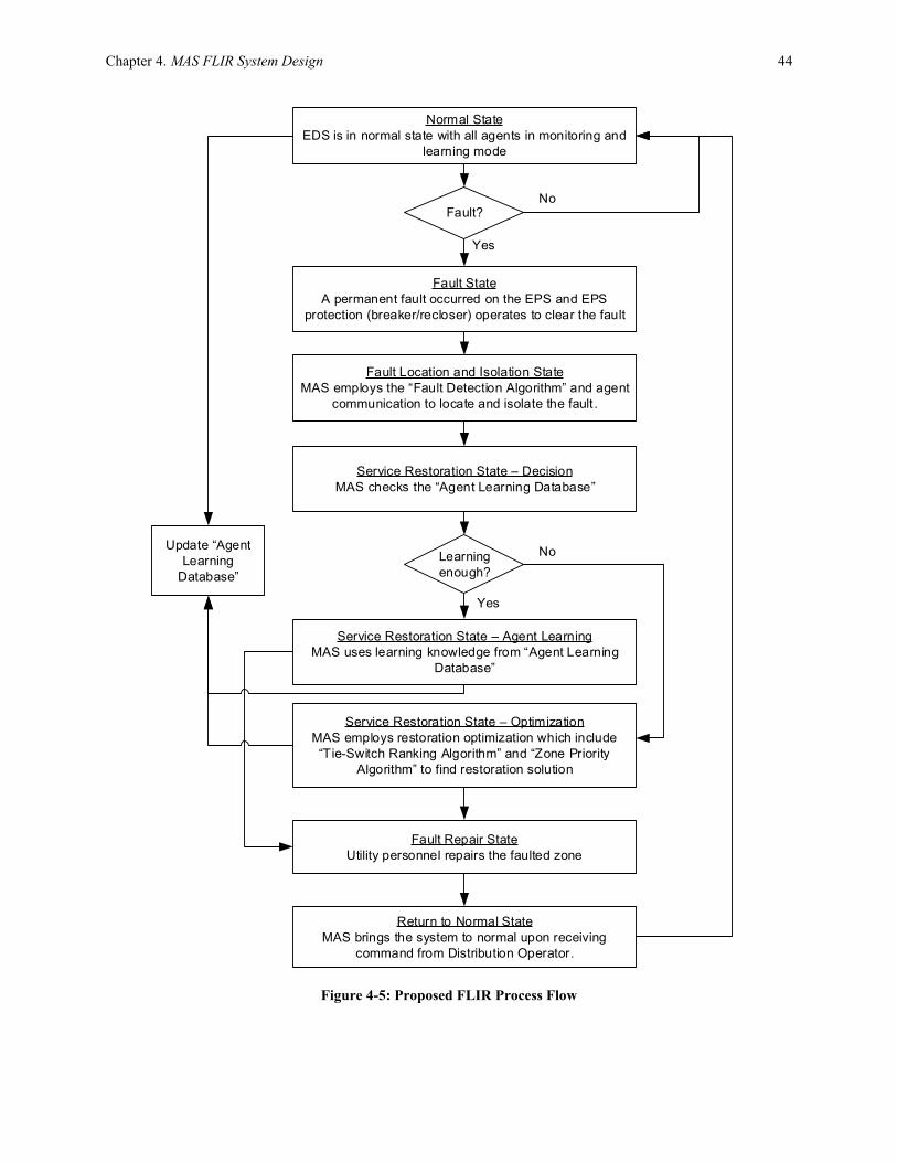
Chapter 4. MAS FLIR System Design 44
Yes
NoFault?
Normal State
EDS is in normal state with all agents in monitoring and
learning mode
Fault State
A permanent fault occurred on the EPS and EPS
protection (breaker/recloser) operates to clear the fault
Fault Location and Isolation State
MAS employs the “Fault Detection Algorithm” and agent
communication to locate and isolate the fault.
Service Restoration State – Decision
MAS checks the “Agent Learning Database”
Learning
enough?
No
Yes
Service Restoration State – Optimization
MAS employs restoration optimization which include
“Tie-Switch Ranking Algorithm” and “Zone Priority
Algorithm” to find restoration solution
Fault Repair State
Utility personnel repairs the faulted zone
Return to Normal State
MAS brings the system to normal upon receiving
command from Distribution Operator.
Update “Agent
Learning
Database”
Service Restoration State – Agent Learning
MAS uses learning knowledge from “Agent Learning
Database”
Figure 4-5: Proposed FLIR Process Flow

45
Chapter 5
Switch Optimization
A novel iterative approach is proposed based on relative reduction in the normalized customer
interruption costs for the optimal switch number and placement problem. An iterative algorithm is
constructed which minimizes the total interruption costs at each step of the analysis to arrive at the
solution. The proposed approach isolates the impacts of varying switch investment and customer
interruption costs that are usually based on outdated utility surveys.
The proposed approach is generalized and works for all kinds of switch types, such as load break
switches, reclosers, fault breaking circuit breakers, etc., with various levels of automation, such as
manually operated, motor operated, remotely operated, etc. Switch investments are isolated in the
approach as these are dependent on switch type and manufacturer, and also vary from country to
country. The proposed iterative algorithm does not rely on absolute customer interruption costs
which are largely dependent on customer damage functions. Customer damage functions usually
are derived based on various survey methods, and they vary greatly from one method of estimation
to the other. This makes determination of optimal switch number and placement very subjective
when the absolute values of customer interruption costs are used in the analysis. Also, this may
lead to unrealistic number of switches as the optimal solution. The proposed iterative algorithm
isolates the impacts of such customer damage functions by employing an approach based on
relative reduction in the normalized customer interruption costs.

Chapter 5. Switch Optimization 46
5.1 Mathematical Problem Formulation
The proposed iterative algorithm for the optimum switch number and placement problem makes
use of customer interruption cost (𝐶𝐼𝐶) [67]. 𝐶𝐼𝐶 responds to the effects of system topology,
interruption duration, load variations, and component random failures. It also recognizes various
customer types and their nonlinear customer damage functions.
DA distribution feeder is divided into a set of Super Sections (SS). SS are formed by logically
grouping a set of actual feeder line segments. Each SS will have load points and the equivalent
load of SS is obtained by summing up individual loads in the SS. SS must be strategically selected
in a way that the created zones of the feeder will have the ability to restore the power from adjacent
feeders in the event of outages. The restoration of the power must not violate the system constraints
such as thermal constraints (conductor or equipment loading limits) and voltage constraints (low
and high voltage issues). DA feeders can be divided into SS with un-equal circuit lengths and
loadings. Each SS is considered as a potential automated switch location in the analysis. A typical
distribution feeder that is divided into SS is shown in Figure 5-1. 𝐶𝐼𝐶 used in this study is
expressed as:
𝐶𝐼𝐶 =∑OCy
k
y=1
=∑ξyly (∑CyzPz
k
z=1
)
k
y=1
(5.1)
𝐶𝑦𝑧 = (𝑅𝑒𝑠𝑧 ∗ 𝑓𝑅(𝑟𝑦𝑧) + 𝐶𝑜𝑚𝑧 ∗ 𝑓𝐶(𝑟𝑦𝑧)+𝐼𝑛𝑑𝑧 ∗ 𝑓𝐼(𝑟𝑦𝑧) ) (5.2)
Where,
𝑘 Total number of Super Sections
𝑂𝐶𝑦 Interruption cost per year due to outages in SS-y
𝜉𝑦 Outage rate (failure/mile-year) of SS-y
𝑙𝑦 Circuit length in miles of SS-y
𝐶𝑦𝑧 Interruption cost of load (residential, commercial and industrial customers) in
$/kW at SS-z due to an outage at SS-y
𝑃𝑧 Total load in kW of SS-z
𝑅𝑒𝑠𝑧 Load percentage of residential customers at SS-z
𝐶𝑜𝑚𝑧 Load percentage of commercial customers at SS-z
𝐼𝑛𝑑𝑧 Load percentage of industrial customers at SS-z
𝑓𝑅 Interruption cost function of residential customers
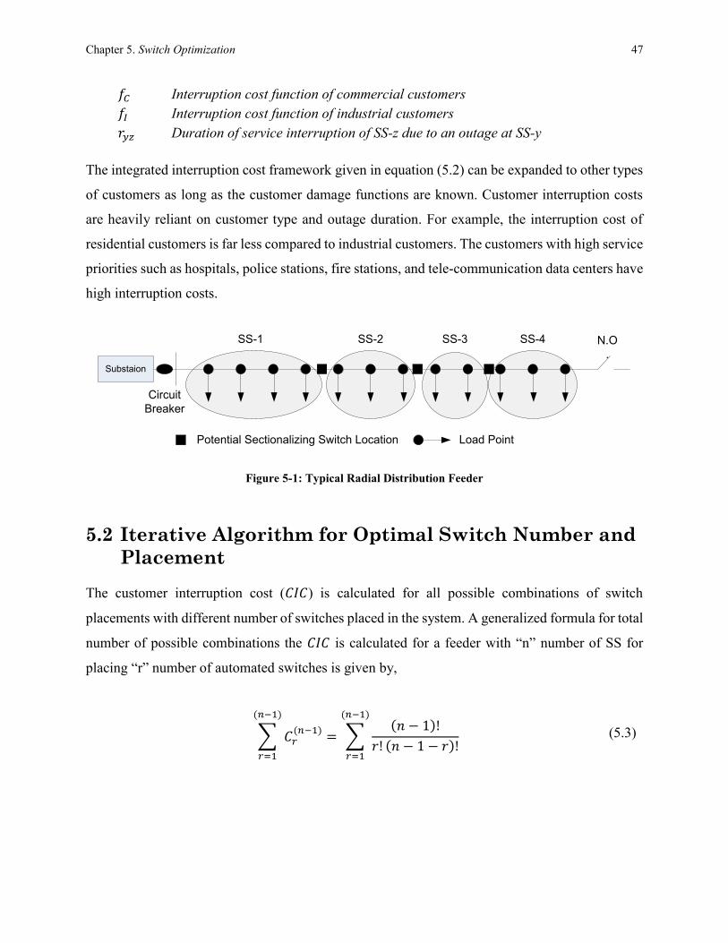
Chapter 5. Switch Optimization 47
𝑓𝐶 Interruption cost function of commercial customers
𝑓𝐼 Interruption cost function of industrial customers
𝑟𝑦𝑧 Duration of service interruption of SS-z due to an outage at SS-y
The integrated interruption cost framework given in equation (5.2) can be expanded to other types
of customers as long as the customer damage functions are known. Customer interruption costs
are heavily reliant on customer type and outage duration. For example, the interruption cost of
residential customers is far less compared to industrial customers. The customers with high service
priorities such as hospitals, police stations, fire stations, and tele-communication data centers have
high interruption costs.
Substaion
N.O
.
Load Point
SS-1 SS-2 SS-3 SS-4
Circuit
Breaker
Potential Sectionalizing Switch Location
Figure 5-1: Typical Radial Distribution Feeder
5.2 Iterative Algorithm for Optimal Switch Number and
Placement
The customer interruption cost (𝐶𝐼𝐶) is calculated for all possible combinations of switch
placements with different number of switches placed in the system. A generalized formula for total
number of possible combinations the 𝐶𝐼𝐶 is calculated for a feeder with “n” number of SS for
placing “r” number of automated switches is given by,
∑ 𝐶𝑟(𝑛−1)
(𝑛−1)
𝑟=1
= ∑(𝑛 − 1)!
𝑟! (𝑛 − 1 − 𝑟)!
(𝑛−1)
𝑟=1
(5.3)

Chapter 5. Switch Optimization 48
The proposed approach significantly reduces the search space and the possible switch
combinations for which 𝐶𝐼𝐶 needs to be computed. The determination of optimal switch number
and location is achieved by the iterative algorithm shown in Figure 5-2.
Start
CICDmir <
CICDmi_limit
End
Yes
No
Divide the feeder into “n” number of Super Sections
Increment
switch
number “r”
by one
Calculate CIC for base case with zero automated switches
(CICb) and normalize it (CICm0)
Start with one automated switch “r”=1
Calculate CIC for all possible switch configurations with “r”
switches
Find the least CIC (CICmr)
Convert CICmr into a normalized index (CICmir)
Calculate reduction in CICmir relative to CICmi(r-1) (CICDmir)
Optimal switch number and location is determined
Optimal number of switches is “r”
Optimal switch placement is placement related to CICmr
Figure 5-2: Iterative Algorithm for Optimal Switch Number and Placement
The steps involved in the process are explained below,
Step 1: Divide the DA feeder into “n” number of SS.
Step 2: Calculate 𝐶𝐼𝐶 for the base case feeder with zero automated switches (𝐶𝐼𝐶𝑏).
Normalize this interruption cost to find cost index (𝐶𝐼𝐶𝑚𝑖0).

Chapter 5. Switch Optimization 49
Step 3: Start the iterative process with one automated switch “r”=1.
Step 4: Calculate 𝐶𝐼𝐶 for all possible switch configurations with “r” switches. The number of
possible combinations is given by equation (5.3).
Step 5: Find the least 𝐶𝐼𝐶 among all the possible switch configurations (𝐶𝐼𝐶𝑚𝑟) with “r”
switches.
Step 6: Normalize 𝐶𝐼𝐶𝑚𝑟 to find cost index (𝐶𝐼𝐶𝑚𝑖𝑟).
Step 7: Calculate reduction in 𝐶𝐼𝐶𝑚𝑖𝑟 relative to 𝐶𝐼𝐶𝑚𝑖(𝑟−1) (𝐶𝐼𝐶𝐷𝑚𝑖𝑟)
Step 8: Check if 𝐶𝐼𝐶𝐷𝑚𝑖𝑟 is less than the iterative threshold (𝐶𝐼𝐶𝐷𝑚𝑖𝑙𝑖𝑚𝑖𝑡). Although this is
a configurable parameter, a value of “8” is used as the threshold in this study.
Step 9: If the condition is FALSE, then increment the number of switches “r” by one and
repeat the process from Step 4.
Step 10: If the condition is TRUE, then the iterative process has identified the optimal number
and placement of switches. The optimal number of switches is “r”. The optimal placement is
the placement corresponding to 𝐶𝐼𝐶𝑚𝑟.
5.3 Test System and Results
The proposed iterative algorithm for optimal switch number and placement is tested on IEEE 34-
bus and IEEE 123-bus test feeders, and Mon Power’s real distribution network involved in WVSC
project.
5.3.1 Test System (IEEE 34-Bus System)
The IEEE 34-bus test feeder is an actual feeder located in Arizona, with a nominal voltage of 24.9
kV. This is a lengthy feeder and assumed to have poor reliability which makes it a perfect candidate
to implement the proposed solution. The data pertaining to feeder load (spot loads and distributed
loads) and line segments (overhead and underground lines) are taken from [68]. The feeder has a
total of 33 line segments with 6 spot loads and 19 distributed loads.
This feeder is strategically divided into seven SS as shown in Figure 5-3. Circuit topography,
customer distribution through the feeder, tie-points and switch locations were taken into account
in the SS selection process. Each SS location is considered to be a potential location for
sectionalizing switch. The information relevant to each SS is furnished in Table 5-1. The
information includes circuit length, load, and failure rate per annum per mile. The circuit length is
different from the actual feeder length in the sense that circuit length is the actual conductor length

Chapter 5. Switch Optimization 50
of line segment. For example, a three phase line segment’s circuit length would be three times the
actual line segment’s length. This helps to account the fault rate to each phase of the line segments
within each SS. As the reliability data for this feeder is not available typical values shown in Table
5-1 are used in the analysis. Each SS is assumed to have a customer mix composed of 50%
residential customers, 25% commercial, and 25% industrial customers.
800
806 808 812 814
810
802 850
818
824 826
816
820
822
828 830 854 856
852
832
888 890
838
862
840836860834
842
844
846
848
864
858
SS-1
SS-2
SS-3
SS-4
SS-5
SS-6
SS-7
Potential Switch Location
Optimal Switch Location
Figure 5-3: IEEE 34-Bus Test Feeder
Table 5-1: IEEE 34-Bus and 123-Bus Test Feeder SS Data
IEEE 34-bus system IEEE 123-bus system
Super
Section
ID
Circuit
Length
(miles)
Load
(kVA)
Failure
Rate /
year-
mile
Circuit
Length
(miles)
Load
(kVA)
Failure
Rate /
year-
mile
SS-1 21.86 80.08 0.06 1.17 335.41 0.59
SS-2 38.20 0.00 0.06 4.67 1406.16 0.59
SS-3 19.07 244.66 0.06 1.02 178.89 0.59
SS-4 37.25 61.37 0.06 1.23 449.38 0.59
SS-5 9.10 521.91 0.06 3.47 626.10 0.59
SS-6 6.61 712.50 0.06 0.31 438.21 0.59
SS-7 4.24 442.92 0.06 1.85 290.69 0.59
SS-8 N/A N/A N/A 1.06 268.33 0.59

Chapter 5. Switch Optimization 51
5.3.2 Test System (IEEE 123-Bus System)
The IEEE 123-bus feeder is considered as a test system to be able to show the computational
efficacy of the proposed solution on a more complicated network. The feeder operates at a nominal
voltage of 4.16 kV and is characterized by overhead and underground lines, unbalanced loading,
four voltage regulators, and shunt capacitor banks. The data pertaining to feeder load and line
segments are taken from [68]. This feeder is strategically divided into eight SS as shown in Figure
5-4. The information relevant to each SS is furnished in Table 5-1. Similar assumptions and data
used for the prior test case are used for this test system.
1
3
4
5 6
2
7 8
12
1114
10
2019
22
21
1835
37
40
135
33
32
31
2726
25
28
2930
250
4847
4950
51
44
45
46
42
43
41
3638
39
66
6564
63
62
60160 67
5758
59
54535255 56
13
34
15
16
17
96
95
94
93
152
9290 88
91 89 87 86
80
81
8283
84
78
8572
73
74
75
77
79
300111 110
108
109 107
112 113 114
105
106
101
102
103104
450
100
97
99
68
69
70
71
197
151
150
61 610
9
24
23
251
195
451
149
350
76
98
76
Potential Switch Location Optimal Switch Location
SS-1
SS-2
SS-3
SS-4
SS-5
SS-6
SS-7SS-8
Figure 5-4: IEEE 123-Bus Test Feeder
5.3.3 Test System (WVSC Distribution System)
Two distribution circuits in Morgantown, WV that were part of WVSC project are selected as the
test system, mainly due to their poor reliability. The geographic view of the Morgantown circuits
is illustrated in Figure 5-5. The two circuits are the West Run #3 Stewarts Street and the West Run
#4 Pine View Circuits. The West Run #3 circuit has 5 normally open tie points with adjacent
circuits. Likewise, West Run #4 has also 5 normally open tie points with adjacent circuits.

Chapter 5. Switch Optimization 52
Therefore, both circuits have many alternative sources which can be utilized to provide service
after a fault condition has been successfully isolated.
Figure 5-5: Geographic View of WVSC Feeders
The West Run substation has two 138/12.5 kV transformers, each with an installed capacity of
33.6 MVA. The Pierpont substation has two 138/12.5 kV transformers with each having a capacity
of 22.4 MVA. There are 327 distribution transformers installed on the West Run #3 circuit and
341 distribution transformers installed on the West Run #4 circuit. The sum of the capacities of
the distribution transformers installed on the West Run #3 circuit is 12,942 kVA, while the sum of
the capacities of the distribution transformers installed on the West Run #4 circuit is 16,670 kVA.
The number of transformers, according to their installed capacities, is illustrated in Figure 5-6.
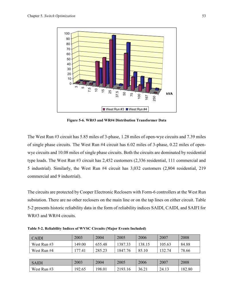
Chapter 5. Switch Optimization 53
Figure 5-6. WR#3 and WR#4 Distribution Transformer Data
The West Run #3 circuit has 5.85 miles of 3-phase, 1.28 miles of open-wye circuits and 7.39 miles
of single phase circuits. The West Run #4 circuit has 6.02 miles of 3-phase, 0.22 miles of open-
wye circuits and 10.08 miles of single phase circuits. Both the circuits are dominated by residential
type loads. The West Run #3 circuit has 2,452 customers (2,336 residential, 111 commercial and
5 industrial). Similarly, the West Run #4 circuit has 3,032 customers (2,804 residential, 219
commercial and 9 industrial).
The circuits are protected by Cooper Electronic Reclosers with Form-6 controllers at the West Run
substation. There are no other reclosers on the main line or on the tap lines on either circuit. Table
5-2 presents historic reliability data in the form of reliability indices SAIDI, CAIDI, and SAIFI for
WR#3 and WR#4 circuits.
Table 5-2. Reliability Indices of WVSC Circuits (Major Events Included)
CAIDI 2003 2004 2005 2006 2007 2008
West Run #3 149.00 655.48 1387.33 138.15 105.63 84.88
West Run #4 177.41 285.23 1847.76 85.10 132.74 78.66
SAIDI 2003 2004 2005 2006 2007 2008
West Run #3 192.65 198.01 2193.16 36.21 24.13 182.80
3 5
7.5
10
15
25
37
.5
50
75
10
0
16
7
25
0
West Run #3
0
10
20
30
40
50
60
70
80
90
100
kVA
Number of TRs / Installed Capacities
West Run #3 West Run #4

Chapter 5. Switch Optimization 54
West Run #4 53.81 102.58 929.50 11.11 17.89 277.28
SAIFI 2003 2004 2005 2006 2007 2008
West Run #3 1.2892 0.3031 1.5807 0.2620 0.2484 2.1538
West Run #4 0.3032 0.3594 0.5079 0.1305 0.1347 3.5252
The WR#3 and WR#4 circuits are strategically divided into 16 SS and 15 SS respectively. Each
SS location is considered to be a potential location for sectionalizing switch. The information
relevant to each SS is furnished in Table 5-3. The load data is only available at the substation
transformer in 15-minute intervals. Therefore, it is assumed that transformer load is distributed to
the feeders evenly proportional with the feeders’ distribution transformer installed capacities. It is
assumed that customer load percentages at all SS are equal to each other, and the customer mix at
the feeder level are used as the input data. The customer load percentages (𝑅𝑒𝑠𝑧, 𝐶𝑜𝑚𝑧 , 𝐼𝑛𝑑𝑧) for
WR#3 and WR#4 feeder used in the analysis are (0.95, 0.04, 0.01) and (0.92, 0.07, 0.00)
respectively.
Table 5-3: WR#3 and WR#4 Feeder SS Data
Super
Section
ID
WR#3 Feeder WR#4 Feeder
Circuit
Length
(miles)
Load
(kVA)
Failure
Rate /
year-
mile
Circuit
Length
(miles)
Load
(kVA)
Failure
Rate /
year-
mile
SS-1 0.95 463 0.0356 0.82 651 0.0364
SS-2 1.20 274 0.0356 1.03 385 0.0364
SS-3 1.19 89 0.0356 1.03 125 0.0364
SS-4 0.98 164 0.0356 0.84 230 0.0364
SS-5 1.35 1249 0.0356 1.16 1755 0.0364
SS-6 2.94 1309 0.0356 5.06 3681 0.0364
SS-7 2.94 1309 0.0356 0.36 482 0.0364
SS-8 0.41 343 0.0356 1.30 960 0.0364
SS-9 1.50 683 0.0356 1.48 1307 0.0364
SS-10 1.72 930 0.0356 1.56 1240 0.0364
SS-11 1.81 882 0.0356 1.76 1875 0.0364
SS-12 2.04 1334 0.0356 1.55 2599 0.0364
SS-13 1.80 1849 0.0356 1.36 1132 0.0364
SS-14 1.58 806 0.0356 1.86 610 0.0364
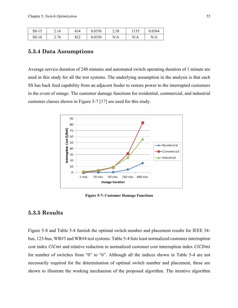
Chapter 5. Switch Optimization 55
SS-15 2.16 434 0.0356 2.38 1155 0.0364
SS-16 2.76 822 0.0356 N/A N/A N/A
5.3.4 Data Assumptions
Average service duration of 240 minutes and automated switch operating duration of 1 minute are
used in this study for all the test systems. The underlying assumption in the analysis is that each
SS has back feed capability from an adjacent feeder to restore power to the interrupted customers
in the event of outage. The customer damage functions for residential, commercial, and industrial
customer classes shown in Figure 5-7 [17] are used for this study.
Figure 5-7: Customer Damage Functions
5.3.5 Results
Figure 5-8 and Table 5-4 furnish the optimal switch number and placement results for IEEE 34-
bus, 123-bus, WR#3 and WR#4 test systems. Table 5-4 lists least normalized customer interruption
cost index 𝐶𝐼𝐶𝑚𝑖 and relative reduction in normalized customer cost interruption index 𝐶𝐼𝐶𝐷𝑚𝑖
for number of switches from “0” to “6”. Although all the indices shown in Table 5-4 are not
necessarily required for the determination of optimal switch number and placement, these are
shown to illustrate the working mechanism of the proposed algorithm. The iterative algorithm

Chapter 5. Switch Optimization 56
stops as soon as the 𝐶𝐼𝐶𝐷𝑚𝑖 index goes below the predefined threshold of “8”. The optimal
number and placement solution for IEEE 34-bus system is “1” and “SS-4”. The optimal number
and placement solution for IEEE 123-bus system is “2” and “SS-2, SS-5”. The optimal number
and placement solution for WR#3 feeder is “3” and “SS-6, SS-10, SS-13”. The optimal number
and placement solution for WR#4 feeder is “3” and “SS-5, SS-7, SS-11”. Increasing the number
of switches beyond the optimal number found here would return minimal reduction in total
customer interruption cost as shown in Figure 5-8 and not worth exploring.
As per the solution provided by the proposed algorithm, installing one sectionalizing switch at SS-
4 on IEEE 34-bus test feeder would reduce the total interruption cost by 69.9% compared to the
base case with no switches. Similarly, installing three sectionalizing switches at SS-6, SS-10, and
SS-13 on WR#3 feeder would reduce the total interruption cost by 74.7% compared to the base
case. Increasing the number of sectionalizing switches beyond the optimal number would result in
relative reduction of interruption costs less than 8%. Figure 5-3, Figure 5-4, and Figure 5-5 mark
optimal placement of switches for IEEE 34-bus, IEEE-123 bus, WR#3, and WR#4 feeders
respectively.
Figure 5-8: Calculated Indices for IEEE 34-Bus, IEEE-123 Bus, WR#3, and WR#4 Feeders
0.0
20.0
40.0
60.0
80.0
100.0
120.0
CIC
mi
an
d C
ICD
mi
Ind
ices
Number of Switches
IEEE_34 CICmi
IEEE_34 CICDmi
IEEE_123 CICmi
IEEE_123 CICDmi
WR#3 CICmi
WR#3 CICDmi
WR#4 CICmi
WR#4 CICDmi

Chapter 5. Switch Optimization 57
Table 5-4: Calculated Indices for IEEE 34-Bus, IEEE-123 Bus, WR#3, and WR#4 Feeders
IEEE 34-Bus Feeder IEEE 123-Bus Feeder WR#3 Feeder WR#4 Feeder
# of
SWs CICmi
CIC
Dmi
Optimal
Switch
Location
CICmi CICD
mi
Optimal
Switch
Location
CICmi CICD
mi
Optimal
Switch
Location
CICmi CICD
mi
Optimal
Switch
Location
0 100.0 N/A N/A 100.0 N/A N/A 100.0 N/A N/A 100.0 N/A N/A
1 30.1 69.9 SS4* 51.6 48.4 SS3 50.3 49.7 SS9 50.3 49.7 SS8
2 22.2 7.9 SS2, SS4 36.8 14.8 SS2, SS5* 34.1 16.2 SS6, SS11 34.2 16.1 SS6,
SS11
3 16.6 5.6 SS2, SS4,
SS5 30.9 5.9
SS2, SS4, SS5
25.3 8.8 SS6,
SS10,
SS13*
26.1 8.1 SS5, SS7,
SS11*
4 13.0 3.5 SS2, SS3,
SS4, SS5 25.6 5.3
SS1, SS2,
SS4, SS5 19.9 5.4
SS5, SS7, SS11,
SS13
19.9 6.1 SS5, SS6,
SS10,
SS12
5 11.0 2.0
SS2, SS3,
SS4, SS5, SS6
23.3 2.4
SS1, SS2,
SS4, SS5, SS6
16.9 3.0
SS4, SS6, SS9,
SS11,
SS13
17.0 2.9
SS5, SS6, SS9,
SS11,
SS13
6 9.9 1.1
SS1, SS2,
SS3, SS4,
SS5, SS6
21.9 1.3
SS1, SS2,
SS4, SS5,
SS6, SS7
14.4 2.5
SS4, SS6, SS8,
SS10,
SS12, SS14
15.2 1.9
SS4, SS5,
SS6, SS9, SS11,
SS13
* Optimal switch location determined by the proposed iterative algorithm.
The number of 𝐶𝐼𝐶 computations increases as the number of switches “r” value increases. The
“r”=1 scenario costs the least processing time as it requires the least number of 𝐶𝐼𝐶 computations
compared to other “r” >1 scenarios. Therefore, the proposed iterative algorithm starts with “r”=1
scenario and stops as soon as the desired solution is achieved. This strategy helps reducing the
search space of the problem. According to equation (5.3), there would be 63, 127, 32767, and
16383 possible combinations of switch placements on IEEE 34-bus, IEEE-123 bus, WR#3, and
WR#4 feeders respectively. The customer interruption cost 𝐶𝐼𝐶 needs to be computed for all the
possible combinations to arrive at a global optimal solution. However, the proposed approach cuts
down the search space drastically to 21, 63, 1940, and 1470 possible combinations for these test
systems and arrives at an optimal solution that satisfies the defined criteria for minimum reduction
in customer interruption costs. This greatly simplifies computational complexity of the problem
and shows efficacy of the proposed solution. Figure 5-9 shows the comparison of search space in
terms of number of 𝐶𝐼𝐶 computations needed for traditional switch optimization approach [67]
and the proposed iterative algorithm.

Chapter 5. Switch Optimization 58
Figure 5-9: Comparison of CIC Calculations between Traditional [67] and Proposed Approaches
0
500
1,000
1,500
2,000
2,500
0
5,000
10,000
15,000
20,000
25,000
30,000
35,000
IEEE-34 Bus IEEE-123 Bus WR#3 WR#4
# o
f C
IC c
alc
ula
tio
ns
wit
h
the
pro
po
sed
ap
pro
ach
# o
f C
IC c
alc
ula
tio
ns
wit
h
tra
dit
ion
al
ap
pro
ach
Test Feeder
# of CIC calculations
with traditional
approach
# of CIC calculations
with the proposed
approach

59
Chapter 6
DG Fault Characteristics
The smart grid initiative is the main cause of increasing DG penetration in electrical distribution
system. As the DG systems become prevalent, the existing protection philosophies get impacted
and warrants for a closer investigation of fault response of various types of DG resources and their
impacts to the existing protection philosophies. The DG resources can be broadly classified into
inverter based and non-inverter based resources. The inverter based sources include photovoltaic,
micro-turbines, fuel cells, and wind turbines with Doubly Fed Induction Generators (DFIG). On
the other hand non-inverter based resources include synchronous and induction generators.
Unlike the non-inverter based DG resources, the inverter based DG resources supply limited fault
currents that could lead to malfunctioning of the distribution network protection system which
largely relies on overcurrent based protection techniques. The absence of mathematical models
and methods to calculate the inverter fault current contribution has been a significant challenge to
the introduction of inverter based DGs [69]. The inverters are actively current limited due to the
low thermal inertia of semiconductor switches, and thus have a small fault current contribution (1-
2 pu) compared to conventional non-inverter based generators (5-10 pu).

Chapter 6. DG Fault Characteristics 60
6.1 Short Circuit Analysis
Short-circuit studies involve calculating available fault levels at various points in the system to
ensure that the protective devices employed in the system are sufficiently sized to interrupt or
withstand short-circuit current. There are several types of faults that can occur on the EDS. The
most common type of fault is single-line-to-ground fault which occurs when one of the phases
comes into contact with alternative current path or ground. A 3-phase fault occurs when all three
phases come into contact with each other and is the least common type of fault. The 3-phase fault
current typically provides the highest available fault current. However, there are situations where
this is not the case.
A fault in a typical EDS behaves very much like a Resistive-Inductive (RL) circuit as shown in
Figure 6-1 with the switch in the closed position. Closing the switch simulates a faulted condition.
XLR
LoadVS
i
Figure 6-1: Circuit Model for Asymmetrical Fault Current
The total fault current ignoring initial value of fault current is given by equation (6.1) which
includes AC current plus the DC offset current. A representation of fault current response is given
in Figure 6-2.
𝑖𝑓(𝑡) = 𝑖𝑎𝑐(𝑡) + 𝑖𝑑𝑐(𝑡) = √2𝑉
𝑍[sin(ωt + α − θ) − sin(α − θ)𝑒−(
𝑡𝑇)] (6.1)
Where 𝑍 = √𝑅2 + XL2, Vs = √2𝑉 sin(ωt + α), θ = tan−1(XL 𝑅⁄ ) ,ω is angular frequency, and
T is the time constant defined by equation (6.2).

Chapter 6. DG Fault Characteristics 61
𝑇 =𝑋𝐿ω𝑅
(6.2)
Figure 6-2: Short Circuit Asymmetrical Current [70]
6.2 Synchronous Machine Fault Response
The short circuit response of a synchronous generator for a fault at its terminal is a decaying pattern
that settles to steady state value after some time. Synchronous machines generally deliver about
six times the rated current for several cycles before decaying to between 400% and 200% of rated
current [71] [72] as shown in Figure 6-3. The external excitation system continues to provide
voltage to the field winding of the generator. The prime mover continues to drive the rotor that
produces the required induced voltage in the stator winding which in turn supplies a continuous
fault current. The steady state fault current value will persist unless interrupted by a protective
device such as a circuit breaker.
The industry has established three reactance variables called sub-transient, transient, and
synchronous reactance [73] to model the short circuit behavior synchronous machines. Sub-

Chapter 6. DG Fault Characteristics 62
transient reactance (Xd′′) determines current during first cycle after fault occurs. This condition lasts
for approximately 0.1 seconds. Transient reactance (Xd′ ) determines current after several cycles.
This condition lasts from 0.5 to 2 seconds. Synchronous reactance (Xd) determines steady state
fault current.
Sub-transient period
Transient period
Steady-state period
Figure 6-3: Synchronous Machine Response to Three Phase Fault
6.3 Induction Machine Fault Response
If a short circuit is applied at the terminal of an induction machine, the current will start out very
high before decaying completely. The induction machines deliver about six times rated current
during this time as shown in Figure 6-4 [72] [73] [74]. Unlike the synchronous machine the fault
characteristic is generated by inertia driving the motor in the presence of the field flux produced
by induction from the stator. During the fault the flux decays due to loss of induction and thus the
fault current decays to zero [73].
The values of transient and synchronous reactance approach infinity under steady-state fault
conditions. Therefore, the induction motors are assigned only a sub-transient value of reactance.
This value varies upward from the locked rotor reactance to account for the decay of the motor
current contribution to the fault. For fault calculations, an induction generator can be treated the
same as induction motor. Wound-rotor induction motors normally operating with their rotor rings

Chapter 6. DG Fault Characteristics 63
short-circuited will contribute short-circuit current in the same manner as a squirrel-cage induction
motor [73].
Figure 6-4: Induction Machine Response to Three Phase Fault
6.4 Inverter based DG Fault Response
Inverter based DGs lack rotating mass that is present with conventional non-inverter based
resources, and they behave dynamically different compared to synchronous or induction machines.
Inverters do not develop inertia to carry fault current based on an electro-magnetic characteristic.
Power electronic inverters have a much faster decaying envelope for fault currents because the
devices lack predominately inductive characteristics that are associated with rotating machines.
The fault response of an inverter based DG depends mostly on its control system rather than its
physical parameters. Moreover, depending on its method of current limiting, an inverter’s fault
response depends on whether the fault is symmetric or asymmetric [75].
6.4.1 Inverter based DG
Figure 6-5 gives a typical representation of an inverter based DG. It consists of DC Power
Generating Unit, DC-DC converter, DC link capacitor, DC-AC inverter, and a LCL filter for grid
interconnection. The DC Power Generating Unit could be a photovoltaic system, fuel cell, micro-

Chapter 6. DG Fault Characteristics 64
turbine, or an energy storage system. The inverter converts the DC voltage into three-phase ac
voltage. The inverter system usually consists a controller that controls the output complex power
of the inverter and ensures the output ac voltage is synchronized with the electric grid voltage. The
DC link capacitor holds the dc output voltage constant during short transients. Therefore, during
transients such as faulted conditions the inverter response mainly depends on the controller [71].
DC Power
Generation Unit
ControllerController
DC-DC
Converter
DC-AC
Inverter
DC link
Capacitor LCL Filter
DC AC
a b c
Three phase
Eletric Grid
Figure 6-5: Inverter based DG
6.4.2 Inverter Control
In order to control the real and reactive power output of inverter, there are two main methods exist.
The first method is known as voltage-mode control and the second method is current-mode control
which is also referred to as multi-loop control.
6.4.2.1 Inverter Voltage-mode Control
Figure 6-6 shows the voltage-mode control of inverter. The real and reactive power are controlled,
respectively, by phase angle and amplitude of the inverter voltage relative to the ac grid voltage.
Therefore, the voltage controlled equivalent circuit shown in Figure 6-6 can be used to represent
the inverter based DG during the transient period for this control method [76] [77]. As indicated
in the figure, simple PI controllers can be used to regulate the output power in the voltage-mode
control scheme. The main shortcoming of the voltage-mode control is that there is no control loop

Chapter 6. DG Fault Characteristics 65
on the inverter line current. Therefore, the inverter is not protected against overcurrent situations,
and the current may undergo large excursions if the power commands are rapidly changed or faults
are taken place in the ac electric grid.
Qo Po
AC Grid
L
Vt Vo
Inverter
Po
Poref
δ
K1(S)Vt
δ
Qo
Qoref K2(S)
Figure 6-6: Grid-connected Inverter Voltage-mode Control
6.4.2.2 Inverter Current-mode Control
The current-mode control scheme has two control loops namely current control loop and power
control loop. The inner current control loop regulates the output current of inverter based DG, and
outer power controller regulates the power output. The current loop is much faster in comparison
with the power control loop. The power controller determines the reference current signal for the
current controller. Figure 6-7 shows the typical representation of inverter current-control scheme
provided in [75]. This setup comprises a three-phase three-leg inverter bridge, a LCL-filter, and a
power controller, an inductor current control loop, a grid synchronization module or a Phase
Locked Loop (PLL), and a current limiting module.
This method of control has an advantage over the voltage-mode control as the current regulation
scheme ensures that the inverter is protected against overcurrent conditions. Other advantages of
the current-mode control include robustness against variations in parameters of the inverter system
and the ac system, superior dynamic performance, and higher control precision. Due to these
benefits, this controls scheme is widely used in most of the inverter based DG applications.

Chapter 6. DG Fault Characteristics 66
PLL
Lc
θ
Lf
Cf
Vt,abcVi,abc
iL,abc it,abc
Power
Controller
Current
Controller
Current
Limiter
PtQt
iL*,dq0
Vi*,abc
abc
dq0
abc
dq0
θiL,dq0
it,dq0
Vt,dq0
Vt,abc
AC GridInner Control Loop
Outer Control Loop
VDC
iDC
0.5VDC
mabc
DC Source
iL*,dq0
iL*,abc
iC,abcPt*Qt*
Figure 6-7: Grid-connected Inverter Current-mode Control
The outer power control loop regulates the output power to given setpoint 𝑆𝑡,𝑟𝑒𝑓 = 𝑃𝑡,𝑟𝑒𝑓 +
𝑗𝑄𝑡,𝑟𝑒𝑓 . According to the instantaneous power theory, the output current references required to
maintain the set output power (𝑃𝑡,𝑟𝑒𝑓and 𝑄𝑡,𝑟𝑒𝑓) and an output voltage of (𝑣𝑡𝑑, 𝑣𝑡𝑞) is given by
equation (6.3).
[𝑖𝑡𝑑,𝑟𝑒𝑓𝑖𝑡𝑞,𝑟𝑒𝑓
] =1
𝑣𝑡𝑑2 + 𝑣𝑡𝑞
2 ∗ [𝑣𝑡𝑑 𝑣𝑡𝑞𝑣𝑡𝑞 −𝑣𝑡𝑑
] ∗ [𝑃𝑡,𝑟𝑒𝑓𝑄𝑡,𝑟𝑒𝑓
] (6.3)
The current control loop regulates the filter inductor current. As shown in Figure 6-7, 𝑖𝐶 = 𝑖𝐿 −
𝑖𝑡 , and 𝑖𝐿,𝑟𝑒𝑓 = 𝑖𝑡,𝑟𝑒𝑓 + 𝑖𝐶 , the inductor reference currents can be found from,
𝑖𝐿,𝑟𝑒𝑓 = 𝑖𝑡,𝑟𝑒𝑓 + 𝑖𝐿 − 𝑖𝑡 (6.4)

Chapter 6. DG Fault Characteristics 67
A low pass filter as shown in Figure 6-8 is used to achieve instantaneous power control that can
produce high inductor current quality. In steady state, the inductor current references are clean DC
signals without any switching harmonics and double harmonic ripple due to unbalance. During
unbalance condition, the grid voltage is characterized by positive, negative, and zero sequence
components.
Pt*
Qt*
Current
Reference
Calculator
Vt,dq0
it,ref
iL,dq0
it,dq0
LPF
iL,ref,dq0 iL*,dq0
Figure 6-8: Power Controller Implementation
If the inverter configuration does not involve neutral wire, the current reference calculation in zero
sequence is not needed. The negative sequence component of current reference appears as a 2𝜔
component in a dq0 reference, and thus has a zero time average, and gets filtered out by the filter.
Therefore, the current reference calculation in the inverter current control is based only on the
positive sequence of the grid voltage (𝑣𝑡𝑝) and hence it only generates a positive sequence current
reference [75]. The inductor current reference to satisfy a given complex power reference is given
in the following equation. The proposed calculation of the current reference depends on the ability
of PLL to accurately estimate the phase angle information of the grid voltage positive sequence
component.
𝑖𝐿,𝑟𝑒𝑓 = 𝑐𝑜𝑛𝑗 (𝑃𝑡,𝑟𝑒𝑓 + 𝑗𝑄𝑡,𝑟𝑒𝑓
3 ∗ 𝑣𝑡𝑝) + 𝑣𝑡𝑝 ∗ 𝑗𝜔𝐶𝑓 (6.5)
The inverter exhibits rather low thermal inertia and they need protection against overcurrent which
is achieved by current limiting. There are several approaches of current limiting. The simplest
method is to implement hard saturation limits in natural reference frame (abc frame) to limit the

Chapter 6. DG Fault Characteristics 68
instantaneous magnitude of the per-phase inductor current reference. This method results in
clipping and distorted waveforms which can introduce power quality issues on the grid side. The
second method involves implementing hard saturation limits in synchronously rotating frame (dq0
frame) when the direct and quadrature axis components exceed a pre-defined threshold. Since the
current reference only possess positive sequence component there will be no 2𝜔 sinusoidal ripple
and no distortion.
The third method, referred to as latched limiting, is similar to the second method with one major
difference where the inductor current is switched to a pre-defined fault current reference (𝑖𝑓) once
the inductor current reference has exceeded the threshold. The last method serves more realistic
applications where the grid interconnected DG units need to supply required amount of fault
current to ensure proper protection of the EDS.
6.4.3 Fault Characteristics and Model of Inverter
According to [71], the inverter fault response under voltage-mode control has a high initial current
overshoot and then the controller brings the current to steady state in a few cycles. Whereas the
inverter under current-model control, the current increases much slower and then decreases back
to the steady-state value rather slowly due to slower power control loop. However, the current in
the current-mode control is well regulated and limited. For photovoltaic inverter based DG, the
fault contribution is really limited due to the fact that these applications do not use the outer power
control loop, or they are very slow [78]. Due to the popularity of the current-mode control scheme,
the research work only focused on studying the inverter fault response under this control.
Faults on the electric grid are characterized by voltage drop at the fault location. When the fault
happens, the power controller increases the inductor current reference to compensate for the drop
in voltage and maintains the set power output. The power controller has a low pass filter with a
cut off frequency of 𝜔𝑐, which makes the inductor current reference to increase in an exponential
manner after a step change in the inverter output voltage at 𝑡 = 𝑡𝑓 and is given by,

Chapter 6. DG Fault Characteristics 69
𝑖𝐿,𝑟𝑒𝑓(𝑡) = 𝑖𝐿,𝑟𝑒𝑓(𝑡0) + (𝑖𝐿,𝑟𝑒𝑓(𝑡𝑓) − 𝑖𝐿,𝑟𝑒𝑓(𝑡0)) ∗ (1 − 𝑒−𝜔𝑐𝑡) (6.6)
The current limiting will be switched on when the magnitude of the current reference exceeds the
predefined threshold (𝑖𝑡ℎ). As per the latched limiting method the current reference will be
switched to pre-defined fault current reference (𝑖𝑓). Usually, the limit is set close to 2 pu and it
causes the fault contribution of the inverter to not exceed 2 pu. The transition of inductor current
reference is given by equation (6.7). Figure 6-9 illustrates a typical fault response of the inverter.
𝑖𝐿,𝑟𝑒𝑓∗ (𝑡) = 𝑖𝑓
𝑡 ≤ 𝑡𝑓 𝑖𝐿,𝑟𝑒𝑓(𝑡0)
𝑡𝑓 < 𝑡 ≤ 𝑡𝑔 𝑖𝐿,𝑟𝑒𝑓(𝑡0) + (𝑖𝐿,𝑟𝑒𝑓(𝑡𝑓) − 𝑖𝐿,𝑟𝑒𝑓(𝑡0)) ∗ (1 − 𝑒−𝜔𝑐𝑡)
𝑡 > 𝑡𝑔 𝑖𝑓
(6.7)
iL,ref (t0)
t0 tf tg t
tiL,ref (tf)
Vt(t0)
Vt(tf)
ith
if
iL,ref (t)
0.33 pu
1 pu
2 pu
3 pu
1 pu
Figure 6-9: Fault Response of an Inverter under Current-mode Control
The fault characteristics of the inverter suggests that inverter with current limiting is equivalent to
a controlled current source of 𝑇𝑐𝑙(𝑠) ∗ 𝑖𝑓 with a parallel filter capacitor admittance 𝑌𝑐𝑓 as illustrated
in Figure 6-10. 𝑇𝑐𝑙(𝑠) is the closed loop transfer function of the control loop. During fault

Chapter 6. DG Fault Characteristics 70
condition, the inverter behaves like a constant current source providing positive sequence current
only. The inverter model in negative and zero sequence has no active sources, and only contain
the parallel capacitor admittance. Figure 6-11 illustrates equivalent circuits of grid-connected
inverter in positivize, negative, and zero sequence. It is important to note that the negative sequence
component of the grid voltage can drive currents through the filter capacitor.
YcfTcl(s)ifVo
io
Figure 6-10: Equivalent Circuit of Grid-connected Inverter with Current Limiting
Vop
iop
Von
ion
Vo0
io0
YcfpTcl(s)if Ycfn Ycf0
Figure 6-11: Equivalent Sequence Network of Grid-connected Inverter

71
Chapter 7
MAS Fault Location & Isolation
SSAs continuously monitor the voltage and current phasor data at their node and neighboring
nodes, and employ Fault Detection Algorithm explained in the following section to autonomously
determine the occurrence of a permanent fault downstream. The SSAs set Permanent Fault Flag
(𝑃𝐹𝑓) status to TRUE when there is a fault downstream. In general, the fault current flows from
source to the fault point when a fault occurs on a radial distribution feeder with no distributed
generation interconnected. However, when EDS has multiple DG interconnections the fault current
is supplied from all these sources, and the fault magnitudes are based on their individual fault
characteristics. Following the fault theory, the fault point always has the deepest voltage sag
compared to the rest of the network and the zone it is associated with sees highest change in the
current flow. This underlying principle is executed by the agent communications to locate the fault
zone of the feeder.
Fault location starts when the feeder recloser or circuit breaker is locked out on a permanent fault
and FA issues the command to locate the fault to its downstream SSAs. All SSAs check if the 𝑃𝐹𝑓
status is TRUE at their node. If the 𝑆𝑆𝐴𝑖 at node-𝑖 identifies that its 𝑃𝐹𝑓 status is TRUE, then 𝑆𝑆𝐴𝑖
determines that the fault is located between its node-𝑖 and downstream node (𝑖 + 1). Once a SSA
finds the fault location, it communicates the fault location to its respective FA. This SSA is also
responsible for fault isolation to make sure the SSWs on both ends of the faulty zone are open. To
achieve this, the SSA sends a control signal to its SSW to open-up and lock in that position. It also
communicates to its downstream SSA to open-up the downstream SSW. This ensures safety of

Chapter 7. MAS Fault Location & Isolation 72
utility crew when they repair the fault in the system. Once the SSA isolates the fault zone, it
communicates to the respective FA indicating to start the service restoration process. The flow
chart of agent communications responsible for the fault location and isolation is shown in Figure
7-1.
Start
FA issues the fault location command to all downstream
SSAs.
SSAi determines that the fault is between its node and the
downstream node.
If any SSAi PFf = TRUE
SSAs check their Permanent Fault Flag PFf status.
Yes
No
Feeder Recloser is Locked Out.
SSAi sends the fault location to the respective FA.
SSAi sends OPEN-LOCK control command to its SSW.
SSAi sends message to its downstream SSA to send a OPEN-
LOCK control command to its SSW.
The SSA sends the fault isolation confirmation to the
respective FA.
A permanent fault occurred.
SSAi receives acknowledgement from the SSWs that they are
open.
End
Figure 7-1: Agent Communication for Fault Location and Isolation

Chapter 7. MAS Fault Location & Isolation 73
7.1 Fault Detection Algorithm
The fault detection algorithm sets the permanent fault flag when it detects a permanent over current
fault. The algorithm consists of four major blocks,
Loss of Voltage (LOV) Detection
Zone Over Current (ZC) Detection
Over Current (OC) Fault Detection
Permanent Fault (PF) Determination
As mentioned above all SSA have access to voltage and current phasor data of its local node. And
through communications they can gather voltage and current phasor information from their
neighboring agents. The SSA captures high fidelity oscillography data for events whenever the
voltage and current quantities go above the programmed thresholds.
Loss of Voltage (LOV)
Detection
Zone Over Current (ZC)
Detection
Over Current Fault
Detection
Permanent Fault
Determination
Fault Flag (Ff)
Permanent Fault Flag (PFf)
Lvx Loss of Voltage Flag (LOVf)
Zone Over Current Flag (ZCf)
LIx
TIx
Tvx
Voltage Phasor Data (Vx)
Current Phasor Data (Ix)
Figure 7-2: Fault Detection Algorithm Blocks

Chapter 7. MAS Fault Location & Isolation 74
7.1.1 Loss of Voltage (LOV) Detection
This block sets the LOV flag (𝐿𝑂𝑉𝑓) of phase-𝑥 when the rms magnitude of phase to ground
voltage 𝑣𝑥 is below the pre-defined voltage level 𝐿𝑣𝑥 for a specified amount of time 𝑇𝑣𝑥 . This
detection is done on a per phase basis and "𝑥" denotes the respective phase "𝑎", "𝑏", and "𝑐". The
chart in Figure 7-3 shows the LOV detection logic. Although the values of 𝐿𝑣𝑥 and 𝑇𝑣𝑥 are
configurable, the algorithm uses typical values of 0.2 pu and 2 cycles respectively.
7.1.2 Zone Over Current (ZC) Detection
This stage of the algorithm calculates the zone current value at each SSA node as indicated in
equation (7.3). The zone current computation at a specific SSA node requires current
measurements from all the DGs present in the zone and from the downstream SSA.
𝐼𝑍𝑥𝑖 =∑𝐼𝐸𝑥𝑗
𝑝
𝑗=1
− ∑𝐼𝐷𝑥𝑗
𝑞
𝑗=1
(7.1)
𝐼𝑍𝑥𝑖 = ± 𝐼𝑆𝑆𝐴𝑥𝑖+1 +∑𝐼𝐷𝐺𝑥𝑘
𝑛
𝑘=1
± 𝐼𝑆𝑆𝐴𝑥𝑖+2 (7.2)
𝐼𝑍𝑥𝑖 = 𝑖𝑓
|𝑣𝑥𝑖 | > |𝑣𝑥
𝑖+1| > |𝑣𝑥𝑖+2|; 𝐼𝑆𝑆𝐴𝑥𝑖+1 +∑𝐼𝐷𝐺𝑥𝑘
𝑛
𝑘=1
− 𝐼𝑆𝑆𝐴𝑥𝑖+2
|𝑣𝑥𝑖 | < |𝑣𝑥
𝑖+1| < |𝑣𝑥𝑖+2|; − 𝐼𝑆𝑆𝐴𝑥𝑖+1 +∑𝐼𝐷𝐺𝑥𝑘
𝑛
𝑘=1
+ 𝐼𝑆𝑆𝐴𝑥𝑖+2
|𝑣𝑥𝑖 | > |𝑣𝑥
𝑖+1| < |𝑣𝑥𝑖+2|; 𝐼𝑆𝑆𝐴𝑥𝑖+1 +∑𝐼𝐷𝐺𝑥𝑘
𝑛
𝑘=1
+ 𝐼𝑆𝑆𝐴𝑥𝑖+2
(7.3)
Where,
𝐼𝑍𝑥𝑖 phase-𝑥 rms current magnitude of zone-𝑖
𝐼𝐸𝑥𝑘 phase-𝑥 rms current magnitude of entering element-𝑘 of zone-𝑖
𝐼𝐷𝑥𝑘 phase-𝑥 rms current magnitude of departing element-𝑘 of zone-𝑖
𝑆𝑆𝑊𝑖+1 upstream SSW of zone-𝑖

Chapter 7. MAS Fault Location & Isolation 75
𝑆𝑆𝑊𝑖+2 downstream SSW of zone-𝑖 𝐼𝑆𝑆𝑊𝑥𝑖+1 phase-𝑥 rms current magnitude measured at 𝑆𝑆𝑊𝑖+1
𝐼𝑆𝑆𝑊𝑥𝑖+2 phase-𝑥 rms current magnitude measured at 𝑆𝑆𝑊𝑖+2
𝐼𝐷𝐺𝑥𝑘 phase-𝑥 rms current magnitude measured at 𝐷𝐺𝑘 location
𝑛 number of DGs present in zone-𝑖 𝑝 number of current entering elements present in zone-𝑖 𝑞 number of current departing elements present in zone-𝑖
|𝑣𝑥𝑖 |, |𝑣𝑥
𝑖+1|, |𝑣𝑥𝑖+2| peak magnitude of phase-𝑥 to ground instantaneous voltage during post-
fault time frame at 𝑆𝑆𝑊𝑖, 𝑆𝑆𝑊𝑖+1, 𝑆𝑆𝑊𝑖+2 respectively.
The zone current change between normal state and fault state can be computed as an index 𝐼𝑍𝐶𝑥𝑖 by
equation (7.4).
𝐼𝑍𝐶𝑥𝑖 =𝐼𝑍𝑥𝑖 (𝐹) − 𝐼𝑍𝑥𝑖 (𝑆)
𝐼𝑍𝑥𝑖 (𝑆)∗ 100 (7.4)
Where,
𝐼𝑍𝐶𝑥𝑖 zone current change index of zone-𝑖
𝐼𝑍𝑥𝑖 (𝐹) rms magnitude of zone-𝑖 current during post-fault
𝐼𝑍𝑥𝑖 (𝑆) rms magnitude of zone-𝑖 current during pre-fault (steady state)
This stage sets the Zone Current flag (𝑍𝐶𝑓) of phase-𝑥 status to TRUE, when the zone current
change 𝐼𝑍𝐶𝑥𝑖 calculated by equation (7.4) is above the pre-defined level 𝐿𝐼𝑥 for a specified amount
of time 𝑇𝐼𝑥 . This detection is done on a per phase basis and "𝑥" denotes the respective phase "𝑎",
"𝑏", and "𝑐". The chart in Figure 7-3 shows the Zone Current detection logic. Although the values
of 𝐿𝐼𝑥 and 𝑇𝐼𝑥 are configurable, the algorithm uses typical values of 200% (or 2 pu) and 2 cycles
respectively.

Chapter 7. MAS Fault Location & Isolation 76
Fault Flag (Ff)
Loss of Voltage Flag (LOVf)
Zone Current Flag (ZCf)
Tvx
Vx
t
TIx
Lvx
LIx
0
Voltage waveform
Zone current change waveform
IZCx
0.2 pu
2 pu
Saturation
1 pu
1 pu
1
Ff
-1 pu
0
0
t
t
Fault Occurrence
Figure 7-3: Fault Detection Algorithm – Voltage and Zone Current Change Waveforms
7.1.3 Over Current Fault Detection
This block determines occurrence of over current fault based on the voltage and zone current
information. The Fault Flag (𝐹𝑓) is set to TRUE when both the 𝐿𝑂𝑉𝑓 and 𝑍𝐶𝑓 flags are TRUE. A
counter namely Fault Counter (𝐹𝐶) keeps track of number of times 𝐹𝑓 is set to TRUE since the last
reset. Each time the 𝐹𝑓 is set to TRUE the 𝐹𝐶 is incremented by one. This is helpful in determining
occurrence of the permanent fault. The logic of the Over Current Fault Detection can be realized
by an AND gate implementation as shown in Figure 7-4.

Chapter 7. MAS Fault Location & Isolation 77
Ff
LOVf
ZCf
Figure 7-4: AND Gate Implementation of Over Current Fault Detection
7.1.4 Permanent Fault Determination
This block determines if there is a permanent over current fault based on the Fault Counter (𝐹𝐶)
value. The block sets the Permanent Fault Flag (𝑃𝐹𝑓) when the 𝐹𝐶 value is equal to a specified
number, which is based on the feeder over current protection employed. The block follows the
rules shown below in setting the 𝑃𝐹𝑓.
𝑃𝐹𝑓 = 𝑖𝑓 𝐶𝐵 𝑝𝑟𝑜𝑡𝑒𝑐𝑡𝑖𝑜𝑛 𝑎𝑛𝑑 𝐹𝐶 = 1; 𝑇𝑅𝑈𝐸
𝑅𝑒𝑐𝑙𝑜𝑠𝑒𝑟 𝑝𝑟𝑜𝑡𝑒𝑐𝑡𝑖𝑜𝑛 𝑎𝑛𝑑 𝐹𝐶 = (𝑛 + 1); 𝑇𝑅𝑈𝐸 (7.5)
Where,
𝑛 number of recloser switching trials; e.g. for a feeder protected by a recloser with three
reclosing trials, the 𝑃𝐹𝑓= TRUE when 𝐹𝐶= 4
7.2 Test System and Modeling
The distribution system associated with WVSC project is used to test the proposed MAS for Fault
Location and Isolation. In order to accurately assess the impact of the short circuit contribution of
different types of DGs and MAS fault location algorithm development and testing, a PSCAD
model of the WVSC distribution grid is developed. A large-scale inverter-based photovoltaic plant,
a synchronous generator, and an induction generator models are developed using the standard
components from the PSCAD library.

Chapter 7. MAS Fault Location & Isolation 78
7.2.1 West Virginia Super Circuit (Base Case)
Figure 7-5 shows a 12.5 kV distribution network of WVSC project fed from two substations
WestRun and Pierpont. The substation transformers ratings are 138/12.5 kV and 33.6 MVA each.
The feeders WR#3 and WR#4 have Distribution Automation and there are 16 automated switches
and 2 reclosers installed in these two feeders. Two feeders from Pierpont Substation and three
other feeders from WestRun substation are used to restore power to the isolated zones of WR#3
and WR#4 feeders.
WESTRUN 138/12.5 kVSUBSTATION
TSW2
TSW4
TSW8
TSW6TSW7
SSW1
SSW3
SSW5
#3
H
#8#4
#5#1
#7
Normally Closed Load Break Switch
Normally Open Load Break Switch
PIERPONT
138/12.5 kV
SUBSTATION
Figure 7-5: Single Line Diagram of WVSC Project 12.5 kV Circuits

Chapter 7. MAS Fault Location & Isolation 79
7.2.1.1 Automated Switches
Figure 7-6 shows a pole-top load break switch installed in the WVSC system. The automated
switches are Cooper DAS-15 type three-phase vacuum switches with 15 kV, 630 A rating. Out of
16 automated switches installed, 7 switches are normally closed and the other 9 switches are used
for reconfiguration and restoration applications. A three-phase current transformer set is embedded
in these switches, and a three phase set of potential transformers are installed externally on one
side of the switch either on the source side or the load side.
Figure 7-6: Pole-top Load Break Switch
7.2.1.2 Substation Reclosers
All circuits originating from the WestRun substation are equipped with reclosers. WR#3 and
WR#4 feeders have 560A, 15.5 kV Cooper electronic reclosers with Form 6 controllers on them.
The recloser with Cooper Form-6 controller shown in Figure 7-7 takes three shots before
permanently locking out on to a permanent fault. Time Current Characteristic (TCC) information
for the installed recloser is given in Table 7-1. The first reclosing operates on A-curve (fast curve)
and the following two reclosing operations operate on D-curve (slow curve). The approximate

Chapter 7. MAS Fault Location & Isolation 80
clearing times for A-curve and D-curve are also listed. The reclosers wait for 60 cycles between
each reclosing operation.
Figure 7-7: Recloser with Cooper Form-6 Controller at WestRun Substation
Table 7-1: Recloser Settings
A curve D Curve
Current (A) 2000 6000 2000 6000
Clearing Time 5 cycles 3 cycles 43 cycles 8 cycles
7.2.1.3 Communication Architecture
The WestRun and Pierpont substations have a Microsol RTU. The West Run RTU communicates
with the Pierpont RTU, the Feeder USP RTUs and the Systems Master Station HMI uses DNP
TCP/IP protocols for communication. The Substation RTU communicates with the feeder
SEL351A relays. The SEL351A relays provide the feeder metering information for all feeders
other than WR#3 and WR#4, which communicate with Cooper Form6 reclosers for their metering
and status data. Hardwired input/output modules on the WestRun RTU provide breaker control for
WR#3 and WR#4 and substation local/remote indication. The RTU at Pierpont substation only
communicates with the WestRun substation RTU, providing information on PP#5 and PP#6

Chapter 7. MAS Fault Location & Isolation 81
feeders. The WestRun RTU has a DNP TCP/IP master to all 14 feeder RTUs and the Pierpont
RTU. A DNP TCP/IP slave communicates with the HMI Master Station.
Each sectionalizing and tie switch point has a Microsol USP RTU communicating with a Microsol
AIM-020 meter, which functions as a meter and a fault (over-current) detection device. The USP
provides control and indication along with communications to the WestRun Microsol substation
RTU. The substation RTU connects to an existing Ethernet 100BaseT (RJ45) access point for
Feeder RTU and Master Station communications using DNP TCP/IP. Two RS485 ports are used
to connect to the SEL351A relays and in the case of WR#3 and WR#4 feeders, the Cooper Form
6s use DNP Serial. The 14 Feeder RTUs connect to a serial to IP converter then to the systems
Ethernet communications system using serial DNP. The Feeder RTU communicates to the AIM
meter using serial Modbus.
7.2.2 West Virginia Super Circuit (FLI Test Case)
In this research, WR#3 feeder is considered as a test system to prove the proposed MAS FLIR
concept. WR#3 feeder has 3 normally closed load break SSWs creating 4 zones and 5 normally
open TSWs. For FLI simulation purpose, four DGs including two synchronous generators, one PV
inverter, and one induction generator are introduced into WR#3 circuit as shown in Figure 7-8.
The generators are simulated to produce different levels of output power to change the DER
penetration level on the WR#3 circuit and to provide different testing scenarios for the proposed
MAS FLI algorithm. All DGs have associated PCC breakers that are completely complaint with
IEEE-1547, i.e., when an islanding condition on the grid occurs, the DG protection opens the PCC
breakers within two seconds of the event to prevent unintentional islanding [79].

Chapter 7. MAS Fault Location & Isolation 82
SSA1
SSA3
SSA5
TSA2
PA3
WestRun Substation
138 kV/12.5 kV
FA3
TSA4
TSA8
TSA7 TSA6
Z1
PA0
PA1
PA5
SG1
PV1
IG1
Z0
Z2
Z3Closed TSW/SSW
Open TSW/SSW
Closed PCC Switch
Open PCC Switch
SG2
SA1
FA4
TSA12
TSA15
SSA14
SSA10
SSA11
TSA9
FA5FA7FA1
Substation
Transformer
33.6 MVA
Pierpont Substation
138 kV/12.5 kV
Closed Recloser
Open Recloser
FA8
Substation
Transformer
33.6 MVA
TSA13 FA5p FA6
SA2
Z1
Z2
Z3
Figure 7-8: Simplified One Line Diagram of WVSC Feeders for MAS FLI
7.2.3 PSCAD Detailed Modeling
Figure 7-9 shows the PSCAD model for WR#3 feeder. Simulation results are calculated based on
per unit values. Distribution lines are modeled based on the positive, negative, and zero sequence
impedance values. Different types of faults such as single line to ground and three phase faults are
modeled with a fault block in PSCAD library. Feeder loads in each zone are modeled as constant
active and reactive power loads. Annual peak demand on WR#3 feeder is modeled as 5 MW at
95% power factor. The simulations are carried out in a discrete mode with a discrete step
simulation time of 16.67 micro-seconds in order to analyze the transient DG fault characteristics.
This results in 1000 samples per cycle simulation readings.

Chapter 7. MAS Fault Location & Isolation 83
Figure 7-9: WVSC Distribution Feeder WR#3 PSCAD Model
7.2.3.1 PV Inverter Model
Figure 7-10 shows the PSCAD core model of the photovoltaic inverter used for this study. It is a
full scale representation of a voltage source inverter with Pulse-Width Modulation (PWM). The
inverter bridge is followed by a LC filter to take out harmonic distortion and allow a controllable
power flow. PWM inverters can quickly cease delivering power to the grid by stopping gating
signals going to the inverter. With switching frequencies of a few kilohertz, this provides tens of
opportunities for disconnection in a single cycle. When dealing with short circuits, the two
decision-making mechanisms for disconnection are under-voltage and over-current measurements.
An important consideration with inverters is the presence of an instantaneous over current relay
(ANSI function #50). Solid-state devices being acutely sensitive to over current, manufacturers
must equip their converters with fast over current sensors to avoid the power bridge to self-destruct
at the first abnormal situation.
The breaker “B” facilitates the connection to the electric grid and has the standard voltage and
frequency protection settings specified in IEEE 1547 standard as shown in Table 7-2 and Table
7-3 .

Chapter 7. MAS Fault Location & Isolation 84
Table 7-2: Interconnection System Response to Abnormal Voltages (rms Voltage)
Voltage Range
(% of the base voltage)
Protective Function
(ANSI #) [80] Maximum Clearing
Time (s)
V < 50 Under voltage (27) 0.16
50 ≤ V < 88 Under voltage (27) 2.00
110 < V < 120 Over voltage (59) 1.00
V ≥ 120 Over voltage (59) 0.16
Table 7-3: Interconnection System Response to Abnormal Frequencies
Frequency Range (Hz) Protective Function
(ANSI #) [80] Maximum Clearing
Time (s)
f > 60.5 Over Frequency (81) 0.16
f < 57.0 Under Frequency (81) 0.16
Figure 7-10: PSCAD Model of PV Inverter
7.2.3.2 Synchronous Generator Model
A simulation model of a synchronous machine based DG unit is developed for the study. The
model represents a small 4 MVA hydro DG based on a synchronous generator. The resulting
PSCAD model is shown in Figure 7-11. The model uses standard components from the PSCAD
library. Multi-mass representation and/or shaft torsional dynamics are neglected in this model

Chapter 7. MAS Fault Location & Isolation 85
since the generator is small and sub-synchronous resonances are not of interest for this study. A
tie-breaker is installed at the connection point of DG and used to disconnect the unit.
The synchronous generator is initialized with the grid steady state conditions such as POI voltage
magnitude and phase angle. The governor and exciter models are eliminated and assumed a
constant field voltage of 1.0 pu to produce terminal voltage of 1.0 pu. The synchronous generator
is made to run at constant speed by locking the rotor at synchronous speed. Thus, there are no
prime mover dynamics involved. To make the model simpler, the machine saturation is disabled
in the model. These simplifications allowed us to focus primarily on the machine dynamics during
the fault event.
Figure 7-11: Synchronous Generator PSCAD Model
7.2.3.3 Induction Generator Model
A simulation model of an induction machine based DG unit is developed for the study. The model
represents a small 1.5 MVA induction generator. The resulting PSCAD model is shown in Figure
7-12. The model uses standard components from the PSCAD library. The induction generator
model can be controlled by specifying either the mechanical torque (TL), or by machine speed (W).
The input “S” is simply a switch signal used to select between two input modes, i.e., when S=0,
input signal TL is selected, and if S=1 input signal W is selected. In order to operate the machine
in speed mode, S=1 is used in the model. A shunt capacitor is used to compensate for the reactive
power demand of the induction generator. A tie-breaker is installed at the connection point of DG
and used to disconnect the unit.

Chapter 7. MAS Fault Location & Isolation 86
Figure 7-12: Induction Generator PSCAD Model
7.3 Fault Location & Isolation Results
7.3.1 Case I - Three Phase Fault in Zone-2
In this scenario a permanent three phase fault (LLL fault) at time 3.82 seconds is considered in
Zone-2 (between SSW3 and SSW5) of WR#3 feeder. The feeder recloser detects the over current
and operates based on TCC information provided in Table 7-1 and locks out. The generator
breakers for SG1, SG2, and IG1 open up five cycles after the fault occurrence, i.e. at 3.90 seconds.
The PV inverter breaker trips at 3.97 seconds following the IEEE 1547 protection settings given
in Table 7-2 and Table 7-3 .
The DGs connected in different zones operate in a grid paralleled mode and supplying feeder loads
during the pre-fault condition. The pre-fault DG output powers and DG instantaneous fault
contributions are shown in Figure 7-13 and Figure 7-14. Table 7-4 summarizes the DG output
power (kW) and fault contribution (pu) measurements. This case represents a 80% DG penetration
scenario as the total DG output power is close to 4.0 MW compared to the total feeder load of 5
MW.
The fault contribution values are per unitized using the individual machine nominal kVA rating as
base. The DG fault contribution values align with the standard fault contribution values of their
machine type that are described in Chapter 6. The PV inverter fault contribution is almost close to

Chapter 7. MAS Fault Location & Isolation 87
2.3 pu right after the fault occurrence and it settles close to 1.7 pu few cycles after the fault
occurrence.
The permanent fault flag (𝑃𝐹𝑓) of SSA3 for three phases are set to TRUE based on the Fault
Detection algorithm. The per-phase zone current change (%) and voltage (kV) waveforms, fault
flag, and permanent fault flag at SSA3 are shown in Figure 7-15. Figure 7-16 shows the per phase
instantaneous voltages at the substation and the SSW nodes. It clearly shows that the magnitude
of voltage during the post-fault condition at the SSW3 location is the lowest in the feeder.
Table 7-5 tabulates the Fault Counter (𝐹𝐶) values and Permanent Fault Flag (𝑃𝐹𝑓) status for SSA1,
SSA3, and SSA5.
The agent communications that takes place for the fault location and isolation is listed below and
shown in Figure 7-17. The SSA3 concludes that there is a three phase fault occurred between its
node and down-stream node and isolates the fault by opening SSW3 and SSW5.
1. Recloser is locked out on a permanent fault (LLL fault).
2. FA3 sends REQUEST performative messages to SSA1, SSA3, and SSA5 to start fault
location.
3. SSA1, SSA3, and SSA5 checks their 𝑃𝐹𝑓 flag status.
4. SSA3 finds out the 𝑃𝐹𝑓 status for all three phases are set to TRUE and it determines that
there is a three phase fault between its node and downstream node, i.e., Zone-2 (between
SSW3 and SSW5).
5. SSA3 sends a INFORM performative message to FA3 to indicate the fault location.
6. SSA3 puts SSW3 in OPEN-LOCK status.
7. SSA3 sends a REQUEST performative messages to SSA5 to put SSW5 in OPEN-LOCK
state.
8. SSA5 sends a ACCEPT performative messages to SSA3 after SSW5 is in OPEN-LOCK
state.
9. SSA3 sends a INFORM performative messages to FA3 to indicate completion of fault
isolation.

Chapter 7. MAS Fault Location & Isolation 88
Table 7-4: DG Output Power and Fault Contribution
# DG Name Zone DG Rating
(kVA)
DG Output Power
(kW)1 Fault Contribution (pu)2
1 SG1 Z0 4000 850 5.1
2 SG2 Z1 4000 850 5.1
3 PV Z2 1500 1000 2.4
4 IG1 Z3 1500 1300 6.4
1. DG output power measured at pre-fault condition.
2. Peak instantaneous fault contribution per unitized using the machine base.
Table 7-5: Fault Counter Value and Permanent Fault Flag Status for LLL Fault in Zone-2
SSA1 SSA3 SSA5
Ph-A Ph-B Ph-C Ph-A Ph-B Ph-C Ph-A Ph-B Ph-C
Fault Counter
(𝑭𝑪) 0 0 0 4 4 4 0 0 0
Permanent Fault
Flag (𝑷𝑭𝒇) FALSE FALSE FALSE TRUE TRUE TRUE FALSE FALSE FALSE
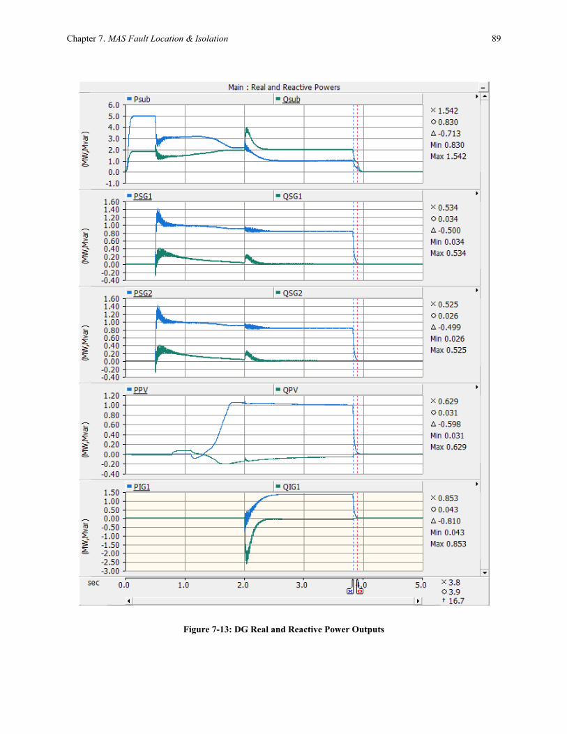
Chapter 7. MAS Fault Location & Isolation 89
Figure 7-13: DG Real and Reactive Power Outputs

Chapter 7. MAS Fault Location & Isolation 90
Figure 7-14: DG Instantaneous Fault Contributions
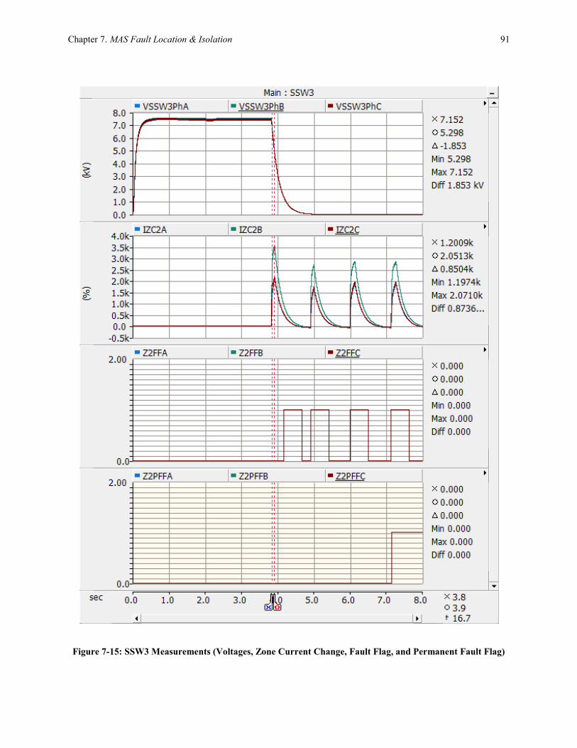
Chapter 7. MAS Fault Location & Isolation 91
Figure 7-15: SSW3 Measurements (Voltages, Zone Current Change, Fault Flag, and Permanent Fault Flag)

Chapter 7. MAS Fault Location & Isolation 92
Figure 7-16: Instantaneous Voltages at the Substation and SSW locations

Chapter 7. MAS Fault Location & Isolation 93
Figure 7-17: Agent Communications for Fault Location and Isolation for LLL Fault in Zone-2
7.3.2 Case II - Line to Ground (LG-A) Fault in Zone-1
In this scenario a permanent phase-A to ground fault (LG-A fault) at time 3.82 seconds is
considered in Zone-1 (between SSW1 and SSW3) of WR#3 feeder. The feeder recloser detects the
over current and operates based on the TCC information provided in Table 7-1 and locks out. The
generator breakers for SG1, SG2, and IG1 open up five cycles after the fault occurrence, i.e. at
3.90 seconds. The PV inverter breaker trips at 4.10 seconds following the IEEE 1547 protection
settings given in Table 7-2 and Table 7-3.
The DGs connected in different zones operate in a grid paralleled mode and supplying feeder loads
during the pre-fault condition. The pre-fault DG output powers and DG instantaneous fault
contribution are shown in Figure 7-18 and Figure 7-19. Table 7-6 summarizes the DG output power
(kW) and fault contribution (pu) measurements. This case represents a 90% DG penetration
scenario as the total DG output power is close to 4.5 MW compared to the total feeder load of 5
MW.

Chapter 7. MAS Fault Location & Isolation 94
The fault contribution values are per unitized using the individual machine nominal kVA rating as
base. The DG fault contribution values align with the standard fault contribution values of their
machine type that are described in Chapter 6. The PV inverter fault contribution is close to 2.3 pu
right after the fault occurrence and it settles close to 1.7 pu few cycles after the fault occurrence.
The permanent fault flag (𝑃𝐹𝑓) of SSA1 for phase-A is set to TRUE based on the Fault Detection
algorithm. The per-phase zone current change (%) and voltage (kV) waveforms, fault flag, and
permanent fault flag at SSA1 are shown in Figure 7-20. Figure 7-21 shows the per phase
instantaneous voltages at the substation and at the SSW nodes. It clearly shows that the magnitude
of voltage during the post-fault condition at the SSW1 location is the lowest in the feeder. Table
7-7 tabulates the Fault Counter (𝐹𝐶) values and Permanent Fault Flag (𝑃𝐹𝑓) status for SSA1,
SSA3, and SSA5.
The agent communications that take place for the fault location and isolation is listed below and
shown in Figure 7-22. The SSA1 concludes that there is a LG-A fault between its node and down-
stream node and isolates the fault by opening SSW1 and SSW3.
1. Recloser is locked out on a permanent fault (LG-A fault).
2. FA3 sends REQUEST performative messages to SSA1, SSA3, and SSA5 to start fault
location.
3. SSA1, SSA3, and SSA5 checks their 𝑃𝐹𝑓 flag status.
4. SSA1 finds out the 𝑃𝐹𝑓 status for phase-A is set to TRUE and it determines that there’s a
LG-A fault between its node and downstream node, i.e., Zone-1 (between SSW1 and
SSW3).
5. SSA1 sends a INFORM performative message to FA3 to indicate the fault location.
6. SSA1 puts SSW1 in OPEN-LOCK status.
7. SSA1 sends a REQUEST performative messages to SSA3 to put SSW3 in OPEN-LOCK
state.
8. SSA3 sends a ACCEPT performative messages to SSA1 after SSW3 is in OPEN-LOCK
state.
9. SSA1 sends a INFORM performative messages to FA3 to indicate completion of fault
isolation.

Chapter 7. MAS Fault Location & Isolation 95
Table 7-6: DG Output Power and Fault Contribution
# DG Name Zone DG Rating
(kVA)
DG Output Power
(kW)1 Fault Contribution (pu)2
1 SG1 Z0 4000 825 2.7
2 SG2 Z1 4000 825 2.7
3 PV Z2 1500 1500 2.3
4 IG1 Z3 1500 1350 6.5
1. DG output power measured at pre-fault condition.
2. Peak instantaneous fault contribution per unitized using the machine base.
Table 7-7: Fault Counter Value and Permanent Fault Flag Status for LG-A fault in Zone-1
SSA1 SSA3 SSA5
Ph-A Ph-B Ph-C Ph-A Ph-B Ph-C Ph-A Ph-B Ph-C
Fault Counter
(𝑭𝑪) 4 0 0 0 0 0 0 0 0
Permanent Fault
Flag (𝑷𝑭𝒇) TRUE FALSE FALSE FALSE FALSE FALSE FALSE FALSE FALSE

Chapter 7. MAS Fault Location & Isolation 96
Figure 7-18: DG Real and Reactive Power Outputs

Chapter 7. MAS Fault Location & Isolation 97
Figure 7-19: DG Instantaneous Fault Contributions

Chapter 7. MAS Fault Location & Isolation 98
Figure 7-20: SSW1 Measurements (Voltages, Zone Current Change, Fault Flag, and Permanent Fault Flag)

Chapter 7. MAS Fault Location & Isolation 99
Figure 7-21: Instantaneous Voltages at the Substation and SSW locations

Chapter 7. MAS Fault Location & Isolation 100
Figure 7-22: Agent Communications for Fault Location and Isolation for LG-A Fault in Zone-1
7.3.3 Miscellaneous Faults
The proposed MAS logic for fault location and isolation has been tested for various fault types in
multiple zones of WR#3 feeder with varying DG penetration levels up to 100% of the feeder load.
Table 7-8 below tabulates 𝐹𝐶 values and 𝑃𝐹𝑓 status for SSA1, SSA3, and SSA5 for various fault
scenarios. This proves that the proposed logic can identify fault type and locate faults in all zones
irrespective of DG penetration on a radial distribution feeder.

Chapter 7. MAS Fault Location & Isolation 101
Table 7-8: Fault Location Results for Miscellaneous Faults
# Fault Scenario
SSA1 SSA3 SSA5
Fault Counter (𝐹𝐶)/ Permanent Fault Flag (𝑃𝐹𝑓)
Ph-A Ph-B Ph-C Ph-A Ph-B Ph-C Ph-A Ph-B Ph-C
0% DG Penetration
1 LLL Fault in Zone-2 0/F 0/F 0/F 4/T 4/T 4/T 0/F 0/F 0/F
2 LG-A Fault in Zone-1 4/T 0/F 0/F 0/F 0/F 0/F 0/F 0/F 0/F
3 LL-AC Fault in Zone-2 0/F 0/F 0/F 4/T 0/F 4/T 0/F 0/F 0/F
50% DG Penetration
1 LLL Fault in Zone-2 0/F 0/F 0/F 4/T 4/T 4/T 0/F 0/F 0/F
2 LG-A Fault in Zone-1 4/T 0/F 0/F 0/F 0/F 0/F 0/F 0/F 0/F
3 LL-AC Fault in Zone-2 0/F 0/F 0/F 4/T 0/F 4/T 0/F 0/F 0/F
100% DG Penetration
1 LLL Fault in Zone-2 0/F 0/F 0/F 4/T 4/T 4/T 0/F 0/F 0/F
2 LG-A Fault in Zone-1 4/T 0/F 0/F 0/F 0/F 0/F 0/F 0/F 0/F
3 LL-AC Fault in Zone-2 0/F 0/F 0/F 4/T 0/F 4/T 0/F 0/F 0/F

102
Chapter 8
MAS Service Restoration
The proposed MAS logic uses the hybrid control philosophy that makes use of both centralized
and decentralized concepts to restore the unfaulty sections of the system. The major advantage of
the hybrid control is that it can achieve optimal restoration solution.
FA waits until the recloser or the CB is completely locked-out on a permanent fault and it receives
fault isolation confirmation from a down-stream SSA to initiate the restoration process. As
explained in the Chapter above, SSAs can autonomously detect the over current faults using the
Fault Detection algorithm. And the fault isolation is achieved by coordinated communications
among SSAs.
The first step in the restoration process is that the FA sends out command signals to all SSAs
except faulted zone SSA to open-up their respective SSWs. Picking up multiple cold (un-
energized) zones at once can lead to severe in-rush currents through substation transformer and
can adversely impact its health. To mitigate this risk of endangering the substation transformers,
the proposed MAS logic follows a sequential energizing process to restore the unfaulty portion of
the faulted circuit. FA divides the faulty feeder into two super zones namely Super Zone-A
(collection of fault-free zones upstream of fault zone) and Super Zone-B (collection of fault-free
zones downstream of fault zone) and handles them individually to restore service.
FA sends communication to all the zone representative SSAs to respond with their pre-fault
loading measurements (three phase quantities of currents, voltages, and net-loading values). SSAs

Chapter 8. MAS Service Restoration 103
communicate with their neighboring SSAs, TSAs, and PAs to compute the respective zone pre-
fault loading information. FA also sends communication to all TSAs and PAs to respond with their
pre-fault measurements (three phase quantities of voltage, current, load, and generation values).
This collective information helps FA to restore power to each un-faulted zone of the Super Zone-
A and Super Zone-B. The FA maintains two lists for the Non-Energized Zones (NEZ) of Super
Zone-A and Super Zone-B, namely NEZ_A and NEZ_B. During the service restoration process
the FA follows strict requirement of maintaining radial nature as most of the electric utilities
operate their distribution system in a radial fashion. Loosing radial nature can greatly impact the
existing protection coordination set-up of the distribution network. Figure 8-1 below shows a
typical distribution feeder with super zones and agent placement.
Microgrid
FASSA1 SSA2 SSA3 SSA4 SSA5 SSA6
TSA1
TSA2
TSA3
PA1
FaultRecloser
Super Zone-A
Substation
Transformer
Super Zone-B
PA2
Figure 8-1: Typical Radial Distribution Feeder with Super Zones
After the above preparation, FA starts the restoration process for Super Zone_A. The FA energizes
the first zone by sending a close command signal to the recloser/CB at the substation. After
successfully energizing the first zone, FA updates the NEZ_A list by deleting the zone that it
recently energized. FA energizes the next zone adjacent to the recently energized zone by sending
a close command signal to the associated SSA. It again updates the NEZ_A list. This process
repeats until all the NEZs in Super Zone_A are energized, or in other words the NEZ_A list is
empty. The logic for restoring the Super Zone_A is shown in the following flow chart.

Chapter 8. MAS Service Restoration 104
Start
FA energizes the first zone by closing feeder recloser
FA updates the NEZ_A list
SSA closes the SSW and updates the NEZ_A list.
Is NEZ_A
list empty?
End
YesNo
Is NEZ_A
list empty?
FA sends the message to its downstream SSA to close its
SSW to energize its zone.
No
Yes
Figure 8-2: Service Restoration of Super Zone-A
8.1 Restoration Formulation
The service restoration problem for Super Zone-B with electrical, operational, and network
constraints can be seen as a constrained multi-objective optimization problem. The objective
functions enforce to restore power to as many loads as possible while maximizing the utilization
of microgrids present in the distribution network, and also try to minimize the number of tie-switch
operations to achieve the target restored network.
A feasible solution is one which satisfies the electrical constraints of KVL and KCL expressed as
three-phase power flow equations. Also, branch current flows, feeder loading, substation
transformer loading, and voltage magnitudes must lie within acceptable operating ranges. The final
reconfigured network should retain the radiality of the system to keep the protection setup of the
distribution network untapped.

Chapter 8. MAS Service Restoration 105
The mathematical formulation of the problem is shown below with its objective functions and
constraints.
Objective Functions:
𝑚𝑎𝑥 𝐽1 =∑𝛾𝑖 ∗ 𝛽𝑖 ∗ (𝑍𝐿𝑖𝑎 + 𝑍𝐿𝑖
𝑏 + 𝑍𝐿𝑖𝑐)
𝑛
𝑖=1
∀𝑖 ∈ 𝑛 (8.1)
𝑚𝑎𝑥 𝐽2 =∑∑𝜇𝐺𝑃𝑖𝑘
𝑚
𝑘=1
𝑛
𝑖=1
∀𝑖 ∈ 𝑛, ∀𝑘 ∈ 𝑚 (8.2)
𝑚𝑖𝑛 𝐽3 = 𝑡𝑛𝑜𝑝𝑠 (8.3)
𝑍𝐿𝑖𝑝 = 𝐿𝐹𝑠𝑠𝑤(𝑖+1)
𝑝 + ∑ 𝐷𝐺𝑖𝑝
𝑛𝐷𝐺
𝑖=1
− 𝐿𝐹𝑠𝑠𝑤(𝑖+2)𝑝 ∀𝑖 ∈ 𝑛𝐷𝐺, 𝑝 ∈ 𝑎, 𝑏, 𝑐 (8.4)
The fulfillment of the objective functions should be obtained by satisfying the following
constraints.
1. Voltage Constraint:
𝑉𝑖𝑚𝑖𝑛 ≤ 𝑉𝑖
𝑝 ≤ 𝑉𝑖𝑚𝑎𝑥 ∀𝑖 ∈ 𝑁, 𝑝 ∈ 𝑎, 𝑏, 𝑐 (8.5)
2. Branch Capacity Constraint:
|𝐼𝑘𝑝| ≤ 𝐼𝑘
𝑚𝑎𝑥 ∀𝑘 ∈ 𝑀, 𝑝 ∈ 𝑎, 𝑏, 𝑐 (8.6)
3. Station Transformer Capacity Constraint:
𝑇𝑘𝑉𝐴𝑖 ≤ 𝑇𝑘𝑉𝐴𝑖𝑛𝑜𝑚 (8.7)
4. Radiality Constraint:
∑𝑇𝑆𝑊𝑖𝑗
𝑛𝑡
𝑗=1
≤ 1 (8.8)

Chapter 8. MAS Service Restoration 106
Where,
𝑍𝐿𝑖𝑎 pre-fault phase-𝑎 net zone-𝑖 load apparent power calculated by equation (8.4)
𝑍𝐿𝑖𝑏 pre-fault phase-𝑏 net zone-𝑖 load apparent power calculated by equation (8.4)
𝑍𝐿𝑖𝑐 pre-fault phase-𝑐 net zone-𝑖 load apparent power calculated by equation (8.4)
𝛽𝑖 weight associated with zone-𝑖 depending on its priority
𝛾𝑖 binary value determining whether zone-𝑖 should be restored or not (1: restored; 0:
not restored)
𝑛 total number of zones to be restored
𝑚 total number of microgrids available in zone-𝑖
𝜇𝐺𝑃𝑖𝑘 PCC status (0=Closed, 1=Open) of microgrid-𝑘 in zone-𝑖
𝑡𝑛𝑜𝑝𝑠 number of tie-switch operations
𝐿𝐹𝑠𝑠𝑤(𝑖+1)𝑝
pre-fault phase-𝑝 apparent power flow through upstream SSW of zone-𝑖
𝐿𝐹𝑠𝑠𝑤(𝑖+2)𝑝 pre-fault phase-𝑝 apparent power flow through downstream SSW of zone-𝑖
𝐷𝐺𝑖𝑝 pre-fault phase-𝑝 apparent power output of DG-𝑖
𝑛𝐷𝐺 total number of DG units including the DGs available in the microgrids present in
zone-𝑖
𝑁 set of all buses in the restored path
𝑉𝑖𝑝 voltage magnitude of phase- 𝑝 at bus-𝑖
𝑉𝑖𝑚𝑖𝑛 minimum allowable voltage magnitude (0.95 pu in our case study)
𝑉𝑖𝑚𝑎𝑥 maximum allowable voltage magnitude (1.05 pu in our case study)
𝑀 set of all branches in the restored path
|𝐼𝑘𝑝| current magnitude of phase- 𝑝 flowing through branch-𝑘
𝐼𝑘𝑚𝑎𝑥 continuous current carrying capacity of branch-𝑘
𝑇𝑘𝑉𝐴𝑖 apparent power flow through station transformer-𝑖
𝑇𝑘𝑉𝐴𝑖𝑛𝑜𝑚 nominal power rating of station transformer-𝑖
𝑇𝑆𝑊𝑖𝑗 status of (1=Closed, 0=Open) tie switch- 𝑗 in the extended zone-𝑖 in the restored
network
𝑛𝑡 number of available tie switches in zone-𝑖
The service restoration problem is an NP-complete problem with discrete and continuous
variables, where the discrete variables are tie and sectionalizing switch statuses and the continuous
variables are the network voltages and current flows. NP-complete problems typically require time
consuming combinatorial optimization algorithms to solve for global optimal solutions [81].
Therefore, the service restoration problem is efficiently solved using the proposed algorithms,
“Tie-Switch Ranking Algorithm” and the “Zone Priority Algorithm”, in this research work.

Chapter 8. MAS Service Restoration 107
Agents in the proposed MAS perceive the system conditions in a continuous manner to learn and
adapt to the new system conditions. Chapter 9 discusses the proposed reinforcement agent learning
methodology used for the service restoration problem. Agent learning is archived in the “Agent
Learning Database”. Each time a successful FLIR action is taken by MAS the “Agent Learning
Database” is updated with the MAS actions and pre and post system state. If there is no feasible
restoration solution exists in the “Agent Learning Database”, the concerned FA/SA performs the
restoration optimization using the “Tie-Switch Ranking Algorithm” and the “Zone Priority
Algorithm” to find out the best possible restoration plan for Super Zone-B.
The proposed MAS follows the logical steps explained in the flow chart shown in Figure 8-3 for
restoring the fault-free zones of Super Zone-B. This logic uses the “Tie-Switch Ranking
Algorithm” and the “Zone Priority Algorithm” that are explained in the following sections. One
unique feature of this restoration logic is that it tries to make use of and account for existing DGs
and microgrids in the restoration process.
The “net load” problem arises due to the presence of DG units on the systems, which means that
the net load that needs to be supplied by the adjacent feeder Tie-switch is larger than the pre-fault
load measurements. The anti-islanding protection trips DG units as soon as a fault condition
appears on the system. And the current DER interconnection standards and regulations do not
allow DGs to re-synchronize to the system until approximately five minutes following restoration
of normal system. It causes the amount of load to transfer may exceed the amount measured just
prior to the fault. The proposed logic accounts for the existing generation of DG units in a fault-
free zone to compute the actual pre-fault net load.
On the other hand microgrids can stay in an islanded mode supplying the local load. It can help
reduce the pre-fault load that needs to be transferred by the adjacent feeder. The PCC breaker is
compliant with IEEE-1547 and UL-1741 anti-islanding standards that ensure that the breaker
opens up as soon as there is a fault on the system to prevent an islanding condition. The breaker
protection is designed to re-synchronize to the grid as soon as the power is restored. And it does
not matter whether the power is restored in normal system configuration by the actual feeder or by

Chapter 8. MAS Service Restoration 108
an adjacent feeder. The proposed MAS makes sure that the PCC breaker is in open condition and
thus the microgrid operates in islanded mode for the entire restoration process. This action helps
to restore power to more fault-free zones by using same amount of adjacent feeder capacity.
FA sends command signals to
the SSAs situated at the ends of
energized portion of the
network to lock the SSWs in
open position to maintain the
radial nature.
Start
FA follows the TRA to select a TSW to close .
Yes
No
FA sends command signal to the respective TSA to close the tie switch and
energize the connected zone.
FA follows the ZPA to pick Left or Right zone for energization.
Is AFC enough to
restore the zone?
FA sends command signal to the respective SSA to close the SSW to energize
the selected zone. Update AFC of the TSW.
FA updates the NEZ_B list.
Is NEZ_B
list empty?
FA sends messages to all PAs to keep the respective PCC Switches in OPEN-
LOCK state during the entire restoration process .
End
Are there
other TSW ?
No
Yes
Yes
No
Yes
Figure 8-3: Service Restoration of Super Zone-B

Chapter 8. MAS Service Restoration 109
8.2 TSW Ranking Algorithm (TRA)
The algorithm is used by FA in prioritizing the TSWs to restore power to the fault-free zones of
the network. The ranking of TSW is determined by two factors: one is the Type of TSW and the
other is Available Feed Capacity (AFC) in kVA or amps. FA requests all of its TSAs to submit
their AFC proposals to compute the TSW rankings. Figure 8-4 shows a typical configuration of a
distribution system fed by two different substations indicating three different kinds of TSWs.
Type-1: This TSW is placed between the feeders fed from same transformer of a substation.
Type-2: This TSW is placed between the feeders fed from different transformers of the
same substation.
Type-3: This TSW is placed between the feeders fed from different substations.
Recloser Sectionalizing
Switch
Tie
Switch
Type-1
Substation
Transformer
Substation A Substation B
Tie
Switch
Type-2
Tie
Switch
Type-3
PCC
Switch
Microgrid
Microgrid
Figure 8-4: Typical Configuration of Distribution System
Usually, as a rule of thumb it is recommended to restore the fault-free zones using TSWs in the
order of Type-1, Type-2, and Type-3. It is evident that using Type-1 TSW for reconfiguration will
result in less line loss and better voltage profile configuration compared to Type-2 TSW. This is
because the effective circuit length of reconfigured network using Type-2 TSW is more than the

Chapter 8. MAS Service Restoration 110
effective circuit length of reconfigured network using Type-1 TSW. Thus, the reconfigured
network using Type-2 TSW will have more line losses and voltage drop compared to the
reconfigured network using Type-1 TSW. Same holds good for Type-2 TSW and Type-3 TSW.
Therefore, Type-1 TSW is given a higher priority compared to Type-2 and Type-3 TSWs.
This algorithm also looks at AFC of TSW besides the “Type” information. AFC is defined as the
load capacity in kVA or amps that can be served by a TSW without violating the system constraints
as mentioned in the optimization formulation. AFC can be computed by running power flows
either at the planning stage using the peak load values or during real time using exact net pre-fault
loadings of the feeder zones after accounting for existing generation by DGs and microgrids. This
is dictated by whether the FA/SA has the power flow computing capability or not.
Another simple way of computing AFC is by using the K-factors for computing the voltage drop
along the restored circuit path. The K-factor is the voltage drop percent down a line that is one
mile long and serving a balanced three-phase load of 1 kVA. Where 𝑙 is the one way distance and
kVA is the actual load of the line [82].
The voltage drop along a line segment is computed by:
𝑉𝑑𝑟𝑜𝑝 = 𝐾𝑓𝑎𝑐𝑡𝑜𝑟 ∗ 𝑘𝑉𝐴 ∗ 𝑙 (8.9)
One must note that AFC calculation using K-factors is an approximate calculation as the K-factor
determination is based on several simplified assumptions that are seldom true for an actual
distribution system. However, in this work we have used K-factors to calculate AFC values of the
system besides the methods that uses power flow. As a future work, we identified the need to
determine the impact of voltage regulating equipment such as shunt capacitor banks and voltage
regulators on the standard K-factors.

Chapter 8. MAS Service Restoration 111
TSW ranking can be mathematically represented as shown below. The rank values are used to rank
the available TSWs. The TSW with highest rank value is ranked number one in the list.
𝑅𝑉(𝑇𝑆𝑊𝑖) = 𝐴𝐹𝐶𝑖 ∗ 𝑊𝑖 (8.10)
Where,
𝑅𝑉(𝑇𝑆𝑊𝑖) Rank value of 𝑇𝑆𝑊𝑖
𝐴𝐹𝐶𝑖 Available Feed Capacity of 𝑇𝑆𝑊𝑖
𝑊𝑖 Weight factor of 𝑇𝑆𝑊𝑖
𝑊𝑖 = 1 for Type-1 switch.
𝑊𝑖 = 0.9 for Type-2 switch.
𝑊𝑖 = 0.8 for Type-3 switch.
8.3 Zone Priority Algorithm (ZPA)
The algorithm is used by the FA to determine which fault-free zone to energize next following the
recently energized fault-free zone using the same TSW. Figure 8-5 shows the fault-free zone
energizing sequence by the ZPA algorithm. This algorithm uses the Left zone and Right zone
terminology as defined below.
1) Left Zone: NEZ situated to the left side (upstream path towards substation source) of the
most recent energized zone.
2) Right Zone: NEZ situated to the right side (downstream path towards the feeder end) of
the most recent energized zone.

Chapter 8. MAS Service Restoration 112
Zone-1 Zone-2 Zone-3 Zone-4 Zone-5
Left Zone Right Zone
Zone to be
energized
Zone-1 Zone-2 Zone-3 Zone-4 Zone-5Left Zone Right Zone
Zone to be
energized
Zone-1 Zone-2 Zone-3 Zone-4 Zone-5
Right Zone
Zone to be
energized
No Left Zone
Zone-1 Zone-2 Zone-3 Zone-4 Zone-5
Right Zone
Zone to be
energized
No Left Zone
Zone-1 Zone-2 Zone-3 Zone-4 Zone-5
No Right ZoneNo Left Zone
Energized Zone Non-Energized Zone
L L
LL
L
L L
L L
L
LOpen Switch Close Switch Locked Switch
Figure 8-5: Zone Energizing Sequence using Zone Priority Algorithm.
This algorithm considers load priority of the zones. The zone that has important loads, such as
hospitals, fire stations, universities, industries, and other commercial loads, is considered to be
high priority zone compared to the other zones. Once a zone is energized, the next zone to be
energized should be of higher priority zone between the Left and Right zones.
If the Left and Right zones carry same load priority, then FA picks the Left zone as default for
energizing activity. This ensures maximum number of zones to be energized as the right most
zones (downstream path towards feeder end) in Super Zone-B always have a TSW availability to
back feed the feeder. If there is no Left zone i.e., if there is an open-locked SSW to the left side of
the most recent energized zone then FA picks the Right zone for energizing activity. If there is no

Chapter 8. MAS Service Restoration 113
Right zone i.e., if there is an open-locked SSW to the right side of the most recent energized zone
then FA skips to another TSW, if available, or stops the restoration process as NEZ_B list might
be empty. All the zones in the WVSC test system are assumed to carry same load priority as per
the guide lines from Mon Power. The guide lines are set by the Public Utility Commission (PUC)
of Mon Power to treat each customer in the system with the same priority and to abide by the
fairness rule.
8.4 Multi-agent Logic for Return to Normal
The system configuration needs to return to normal configuration once the fault in the system is
fixed. This process is handled by the FA. FA waits for the Return to Normal command from the
distribution operator, and as soon as it receives this command it starts communicating with its
SSAs and TSAs to bring the system back to normal operating conditions.
FA communicates to TSAs, which have the closed TSWs that were used for restoration, to open
the TSWs. Similarly, FA communicates with all PAs to lift LOCK condition on microgrid PCC
switches. This ensures that PCC switch will be able to re-synchronize to the grid once the feeder
configuration returns to normal and energized. FA communicates to all SSAs to open their SSWs
to be prepared for the normal operation. Once FA receives confirmation from all TSAs, SSAs, and
PAs, it sends command signal to close the recloser or circuit breaker to energize the first zone of
the feeder. Once the zone is energized, FA will send the command signal to downstream SSA to
close its SSW energizing its zone. FA repeats this procedure until all the zones are energized and
system is brought back to normal configuration. The Return to Normal logic is shown in the
following flowchart.

Chapter 8. MAS Service Restoration 114
Start
FA communicates to SSAs to open SSWs
FA sends command signal to downstream SSA to close its SSW energizing its
zone
Last SSA
reached?
FA sends command signal to close the recloser energizing the first zone .
Yes
No
FA communicates to TSAs to open TSWs
Operator issues the Return to Normal Command
FA communicates to PAs to lift LOCK condition on PCC Switches
End
Figure 8-6: MAS Logic for Return to Normal

115
Chapter 9
Reinforcement Agent Learning
The agents in a Multi-Agent System can be programmed with behaviors designed in advance,
however, it is often necessary that they learn new behaviors online, such that the performance of
the agent or of the whole Multi-Agent System gradually improves [83]. The static behaviors
programmed in agents might not be sufficient to address all the issues of dynamic environment,
and learning becomes a crucial aspect of Multi-Agent System design.
The agents learns by trial-and-error interactions with its dynamic environment using reinforcement
learning. At each time step, the agent perceives the complete state of the environment and takes
an action, which causes the environment to transit into a new state. The agent receives a scalar
reward signal that evaluates the quality of this transition. The simplicity and generality of the
setting makes RL attractive for Multi-agent learning.
Agent learning can greatly benefit the service restoration problem by providing reconfiguration
solutions directly from its past experiences. Agents knowledge will be continuously updated online
using the real-world experiences as the system takes action and receives the reinforcement signals
from the system. The service restoration with RL can be realized with less number of
communications among the agents and with minimal amount of time, hence improving the overall
system reliability.
We used a famous reinforcement learning algorithm, Q-learning, for the agent learning of the
service restoration problem. Being based on dynamic programming, this off-policy method

Chapter 9. Reinforcement Agent Learning 116
theoretically can converge to the optimal reconfiguration [54] [41]. As Q-learning is an online
approach, it can be deployed within a real electric distribution system, where the algorithm can not
only fine-tune itself over time, but also re-adapt in the presence of non-stationary EDS
environment. This makes Q-learning less susceptible to system drift due to configuration and
equipment changes.
9.1 Q-Learning
Q-Learning algorithm is a reinforcement learning algorithm proposed by Watkins to deal with
Markov Decision Process (MDP). In a MDP, the main objective of the agent is to find its action
so as to maximize the sum of discounted expected rewards as given by the value function,
𝑉(𝑠, 𝜋∗) = 𝑚𝑎𝑥𝑎 𝑟(𝑠, 𝑎) + 𝛾 ∑𝑝(𝑠′|𝑠, 𝑎)
𝑠′
𝑉(𝑠′, 𝜋∗) (9.1)
Where 𝑟(𝑠, 𝑎) is the reward for taking action 𝑎 to transition from the current state 𝑠 to next state
𝑠′, 𝛾 ∈ [0; 1) is the discount factor, 𝑝(𝑠′|𝑠, 𝑎) is the probability of transitioning into state 𝑠′ after
taking action 𝑎 at state 𝑠, and 𝜋∗ is the optimal strategy that satisfies the equation (9.1).
In Q-Learning agents do not know the reward function or the state transition probabilities, hence
this is a form of model-free reinforcement learning. An action-value function or Q-function can be
defined such that,
𝑄∗(𝑠, 𝑎) = 𝑟(𝑠, 𝑎) + 𝛾 ∑𝑝(𝑠′|𝑠, 𝑎)
𝑠′
𝑉(𝑠′, 𝜋∗) (9.2)
𝑄∗(𝑠, 𝑎) is the total discounted reward of taking action 𝑎 at state 𝑠 and then following optimal
policy thereafter. Comparing equations (9.1) and (9.2) we have,
𝑉(𝑠, 𝜋∗) = 𝑚𝑎𝑥𝑎𝑄∗(𝑠, 𝑎) (9.3)

Chapter 9. Reinforcement Agent Learning 117
The problem of finding optimal policy 𝜋∗ is simply to identify the action that maximizes 𝑄∗(𝑠, 𝑎).
If we know 𝑄∗(𝑠, 𝑎), we can find the optimal policy to take under any state. Therefore, the problem
is finding Q-values for each state.
9.1.1 Learning
Agents maintain the Q-values for each and every possible state and action pair. Since the Q-
Learning is an iterative method, the Q-values are initially assumed to be zero or some arbitrary
small values. Q-learning provides a simple updating procedure to approximate the Q-value from
empirical examples obtained from the actual experiences,
𝑄𝑡+1(𝑠𝑡, 𝑎𝑡) = (1 − 𝛼) 𝑄𝑡(𝑠𝑡, 𝑎𝑡) + 𝛼 [𝑟𝑡 + 𝛾 𝑚𝑎𝑥𝑎𝑄𝑡(𝑠𝑡+1, 𝑎𝑡) − 𝑄𝑡(𝑠𝑡, 𝑎𝑡)]
(9.4)
Where 𝛼 ∈ [0; 1) is the learning rate which determines how much the new experiences affect the
old Q-value. A factor of 0 will make the agent not learn anything, while a factor of 1 would make
the agent consider only the most recent information. The learning rate is typically time varying
and decreasing with time. Watkins and Dayan [56] proved that the sequence generated by (9.4)
converges to 𝑄∗ under the assumption that all states and actions have been visited infinitely often
and the learning rate satisfies certain constraints.
9.1.2 Exploration
Exploration is the action selection mechanism selected by agent to transition into future states.
There are three popular exploration techniques mentioned in the literature, 𝜖-greedy, Roulette, and
Boltzmann distribution. The Q-values of any given state represents the effectiveness of the action,
with higher values corresponding to better actions. Thus under a greedy policy, the best action to
apply to a given state is simply,
𝑎 = 𝑎𝑟𝑔𝑚𝑎𝑥𝑎′𝑄(𝑠, 𝑎′) (9.5)
As an immediate consequence of this greedy strategy, actions that are chosen in such a manner the
agent reaches to its final state optimally. This is a desirable outcome, however, the greedy rule can

Chapter 9. Reinforcement Agent Learning 118
obtain the best actions after the algorithm has explored a sufficient number of possible
configurations and converged towards the actual Q-values. In order to explore the effectiveness of
other actions during the learning stages of the algorithm, action selection must be carried out in a
probabilistic manner. The Boltzmann distribution function to assign a probability 𝑝(𝑎|𝑠𝑡) to the
actions in order to create a graded function of estimated value:
𝑝(𝑎|𝑠𝑡) = 𝑒𝑥𝑝
𝑄𝑡(𝑠𝑡,𝑎)𝜏⁄
∑ 𝑒𝑥𝑝𝑄𝑡(𝑠𝑡,𝑎𝑖)
𝜏⁄𝑚𝑖=1
(9.6)
The quantity 𝜏 is called the temperature parameter, which adjusts the randomness of action
selection. An agent selects actions randomly when 𝜏 is high, and it selects actions based on greedy
strategy when 𝜏 is low. Therefore, in order to make the algorithm exploratory, 𝜏𝑜 is initialized with
a high value and decreased gradually towards a final low value 𝜏∝. At the end of the predetermined
number of iterations, the greedy strategy is applied to obtain a restoration action necessary to
restore the maximum possible power with least number of switching operations.
9.2 Learning Methodology for Service Restoration
The main goal of Multi-Agent System using Q-learning is to restore power to as many fault-free
zones as possible with minimum number of switching operations while utilizing available
distributed generation and microgrids in the system. The agent has a learning module that consists
of learning database, action selection module, reward module, and Q-updating module. As the
name suggests, the learning database maintains Q-values for each possible state of the system,
action selection module implements a specific strategy to select the best possible action that
maximize the reward, reward module computes the scalar reward, and Q-update module updates
the Q-values after each successful exploration of an episode.
9.2.1 Reinforcement Reward Function
Let the set of all possible states of the system be denoted as 𝑆 = 𝑠1, 𝑠1… , 𝑠𝑛 and the set of all
actions available at a random state 𝑠𝑘 be denoted as 𝐴𝑘 = 𝑎𝑘1, 𝑎𝑘1… , 𝑎𝑘𝑛. Each action entails

Chapter 9. Reinforcement Agent Learning 119
either the opening or the closing of a tie switch or sectionalizing switch. The Q-learning is
implemented in such a way that switching operations that cut off power to system zones are
ignored. Therefore, in any state a smaller number of distinct actions in 𝐴𝑘 are explored by the
algorithm.
The electric distribution system can be viewed as a Finite State Model (FSM). At any random state
𝑠𝑘, any available actions in 𝐴𝑘, transitions the system into a new state 𝑠′𝑘. The reinforcement signal
or the reward function is then defined as an increment in the restoration objective function given
by,
𝑅(𝑠𝑘, 𝑎𝑘𝑖) = Δ 𝒥(𝑠𝑘, 𝑎𝑘𝑖) = 𝒥(𝑠′𝑘) − 𝒥(𝑠𝑘)
(9.7)
𝒥 =∑𝛾𝑖 ∗ 𝛽𝑖 ∗ (𝑍𝐿𝑖𝑎 + 𝑍𝐿𝑖
𝑏 + 𝑍𝐿𝑖𝑐)
𝑛
𝑖=1
∀𝑖 ∈ 𝑛 (9.8)
Where 𝒥 is the service restoration objective function defined in section 8.1. The restoration action
that would yield maximum power restored will have a large reward. The reward function in (9.7)
can be modified to add additional restoration performance metrics such as percent voltage drop,
line losses, and tie-switch operations. The modified reward signal is given by,
𝑅(𝑠𝑘 , 𝑎𝑘𝑖) = 𝒲𝑗 ∗ (𝑃𝑟𝑒𝑠𝑡𝑜𝑟𝑒𝑑𝑃𝑜𝑢𝑡𝑎𝑔𝑒
) + 𝒲𝑣𝑑 ∗ (1 − 𝒱𝑑𝑟𝑜𝑝) + 𝒲𝑝𝑙 ∗ (1 −Δ 𝑃𝑙𝑜𝑠𝑠𝑃𝑓𝑒𝑒𝑑𝑒𝑟
) + 𝒲𝑡𝑛 ∗ (1 − 𝓉 ∗ 𝑡𝑛𝑜𝑝𝑠) (9.9)
Where 𝑃𝑜𝑢𝑡𝑎𝑔𝑒 is the total power outage due to the fault condition in the system, 𝑃𝑟𝑒𝑠𝑡𝑜𝑟𝑒𝑑 is the
amount of power restored, 𝒱𝑑𝑟𝑜𝑝 is the percent voltage drop calculated from feeder breaker to the
end point of the final zone that is restored due to tie switch, Δ 𝑃𝑙𝑜𝑠𝑠 is the change in line loss for
restored network before and after the restoration, 𝑃𝑓𝑒𝑒𝑑𝑒𝑟 is the feeder load of the restored network,
𝓉 = 0.1 is the scaling factor for number of tie switch operations, and 𝒲𝑗, 𝒲𝑣𝑑, 𝒲𝑝𝑙, 𝒲𝑡𝑛 ∈ [0; 1]
are the reward weights associated with performance parameters, load restoration, voltage drop,
line loss, and number of tie-switch operations respectively.

Chapter 9. Reinforcement Agent Learning 120
𝒲𝑗, 𝒲𝑣𝑑, 𝒲𝑝𝑙, 𝒲𝑡𝑛 weights can be configured in a way that we can prioritize agent learning with
respective to any specific performance parameter or a combination of the parameters. In this work
the weights are assumed as 𝒲𝑗 = 1, 𝒲𝑣𝑑 = 0.9, 𝒲𝑝𝑙 = 0.1, 𝒲𝑡𝑛 = 1 to give the highest priority
to restore power to as much load as possible using minimum number of tie switch operations while
supplying good voltage profile. The agent learning is least impacted by line losses as it is a
manageable operational parameter.
9.2.2 Q-Value Matrix
The feeder agent or the substation agent maintains the Q-value repository of all the information
learned through its own experiences in the agent learning database. FAs can use the learning
database for decision making and see how the past actions worked. The Q-value repository for the
service restoration problem is a 2-D matrix and the size of the matrix depends on number of feeder
zones, available tie switches, and sectionalizing switches. A typical Q-value matrix along with its
associated switch combination matrix ℋ𝐹𝐴ℎ is given by,
𝒬𝐹𝐴ℎ(𝑠𝑘, 𝑎𝑘𝑖) = [𝒬11 ⋯ 𝒬1𝑧⋮ ⋱ ⋮𝒬𝑛1 ⋯ 𝒬𝑛𝑧
] (9.10)
ℋ𝐹𝐴ℎ(𝑠𝑘, 𝑎𝑘𝑖) = [
ℋ11 ⋯ ℋ1𝑥
⋮ ⋱ ⋮ℋ𝑛1 ⋯ ℋ𝑛𝑥
] (9.11)
Where 𝑧 is number of zones in the feeder ℎ monitored by the feeder agent 𝐹𝐴ℎ, 𝑥 is total number
of tie switches 𝑥𝑡 and sectionalizing switches 𝑥𝑠 present in feeder ℎ including the feeder breaker
or recloser, and 𝑛 = 2𝑥 is number of possible switching combinations of 𝑥 number of tie switches,
sectionalizing switches, and feeder breaker or recloser. ℋ𝑛𝑥 is switch status index (1-close, 0-
open) indicating the status of 𝑥 tie switch, sectionalizing switch, or feeder recloser. 𝒬𝑛𝑧 represents
the accumulated reward for 𝐹𝐴ℎ to choose the switching action specified in row vector of switch
combination matrix ℋ𝐹𝐴ℎ = (ℋ𝑛1 ⋯ ℋ𝑛𝑥) for service restoration of a fault in zone 𝑧. The Q-

Chapter 9. Reinforcement Agent Learning 121
value matrix is a sparse matrix since only a handful number of switching combinations are feasible
for service restoration for a fault in a feeder zone.
For any state 𝑠𝑘, there is at least one action 𝑎∗ that has the largest reward and Q-value among the
possible actions for a zone restoration.
𝒬(𝑠𝑘, 𝑎∗) > 𝒬(𝑠𝑘, 𝑎)
(9.12)
9.2.3 Q-Update Rule
The Q-values in the matrix repository explained in the above section are updated after a successful
implementation of an action using the update rule,
𝑄𝑡+1(𝑠𝑡, 𝑎𝑡) = (1 − 𝛼) 𝑄𝑡(𝑠𝑡, 𝑎𝑡) + 𝛼 [𝑄′(𝑠𝑡, 𝑎𝑡)]
(9.13)
Where 𝑄 and 𝑄′ are the last Q-value and the most recently obtained Q-value, 𝛼 ∈ [0; 1) is the
learning rate which determines how much the new experiences affect the old Q-value. A factor of
0 will make the agent not learn anything, while a factor of 1 would make the agent consider only
the most recent information. We can make use of changing the learning rate to ensure the learning
efficiency. The incremental change in Q-values, denoted by Δ𝒬, should reduce progressively if Q-
learning converges and conversely if Δ𝒬 is oscillating and diverges.
9.2.4 Action Selection Strategy
FA selects the switching actions based on the deterministic greedy strategy at a given state with
Q-matrix values. If there are more than one switching solutions available, according to the greedy
policy, the FA selects the switching action that maximizes the total reward,
𝑎 = 𝑎𝑟𝑔𝑚𝑎𝑥𝑎′𝑄(𝑠, 𝑎′) (9.14)

Chapter 9. Reinforcement Agent Learning 122
The higher Q-values suggests to select the corresponding action with confidence. In the proposed
service restoration Q-learning framework with the assumed weights and parameters, if 𝑄(𝑠, 𝑎′) ≥
2.85 means that the corresponding set of switching actions specified in switch combination matrix
ℋ𝐹𝐴ℎ can restore power to all fault free zones with a voltage drop less than 5% and a line loss less
than 5%.
The greedy strategy obtains the best switching action choices if the algorithm has explored
sufficient number of possible actions. If not, this action selection strategy might stay in a local
optimum point. Therefore, it is imperative to explore all possible remedial actions using
simulations to prevent the system trapping in local minimas.
9.2.5 Q-Learning Process Flow
The main advantage of the Q-learning is that the agents' knowledge will be continually updated
online as the system takes action and receives the reinforcement learning signals from power
system. However, the agents require initial knowledge of Q-values for possible events in the
system before field deployment. The initial learning database can be built by off-line learning
methodology through simulation models for each scenario. In this manner, Multi-Agent System
will have a primary knowledge about scenarios it might encounter in the future.
The overall process flow of the proposed Q-learning approach is shown in Figure 9-1. FA stores
the Q-values and corresponding switch combination matrix ℋ𝐹𝐴ℎ entries in memory for events
that have been encountered previously, or for events that might likely to happen in future using
off-line learning approach.
For a fault in EDS, FA looks into agent learning database to see if Q-values are present. If so, the
optimal action based on greedy strategy in equation (9.14) is selected to perform switching actions
specified in corresponding switch combination matrix ℋ𝐹𝐴ℎ . The EDS returns the reinforcement
obtained by applying these switching actions based on the reward function in equation (9.9). And
the stored Q-values are updated as mentioned in equation (9.13) and the state is updated to
represent the current state. In this manner the Q-values can benefit from continual online updates
using the sequence of reinforcement signals obtained directly from the EDS.

Chapter 9. Reinforcement Agent Learning 123
If learning is not present for a fault scenario, the service restoration is solved using the optimization
approach with TRA and ZPA algorithms. Once the solution is implemented in EDS, the Q-values
for this particular scenario will be initialized in the FA’s memory.
Start
Initialize Q-values
Pick feasible exploratory action in switch
combination matrix
Simulate EDS with action
Obtain reinforcement signal and update
Q-values
Q-values
converged?
All likely fault
scenarios explored?
Pick a likely fault scenario and feeder
loading state
End
YES
NO
YES
NO
Start
Pick action based on greedy strategy in
switch combination matrix
Implement action on EDS
Obtain reinforcement signal and update
Q-values
Fault in system?
End
YES
NO
YES
NO
Learning exists?
Perform service restoration based on
Optimization and add an Q-value entry
Off-line Q-Learning On-line Q-Learning
Figure 9-1: Q-Learning Process Flow for Service Restoration

124
Chapter 10
Service Restoration Results
The distribution system associated with WVSC project is used to test the proposed MAS for
Service Restoration. The WVSC distribution system is simulated by using MATLAB® Simpower®
toolbox and also CYME® for voltage drop studies, all agents are implemented using S-functions
in Simulink. This simulation set-up needs no interface between MAS and power system model.
This advantage provides a simpler and more accurate simulation model. During the simulation, S-
functions use a special calling syntax called the S-function API that enables you to interact with
the Simulink engine and synchronize the simulation of agents with power system model.
10.1 WVSC System (Base Case)
Figure 7-5 shows the 12.5 kV distribution network of WVSC project fed from two substations
WestRun and Pierpont. As mentioned in Chapter 7, the feeders WR#3 and WR#4 have Distribution
Automation with 16 automated switches and 2 reclosers installed. The study concerns total of six
feeders originating from WestRun substations and two feeders originating from Pierpont
substation. Table 10-1 provides the peak load data for these feeders that are used to run the load
flow studies for the base case.
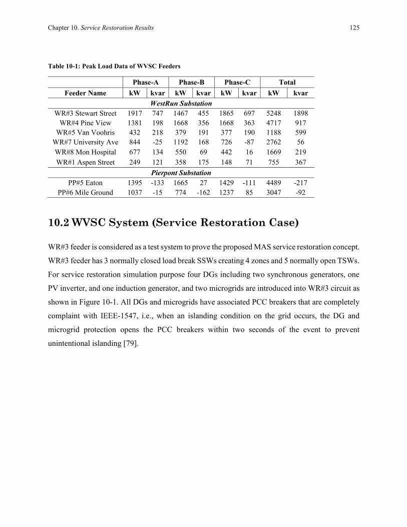
Chapter 10. Service Restoration Results 125
Table 10-1: Peak Load Data of WVSC Feeders
Phase-A Phase-B Phase-C Total
Feeder Name kW kvar kW kvar kW kvar kW kvar
WestRun Substation
WR#3 Stewart Street 1917 747 1467 455 1865 697 5248 1898
WR#4 Pine View 1381 198 1668 356 1668 363 4717 917
WR#5 Van Voohris 432 218 379 191 377 190 1188 599
WR#7 University Ave 844 -25 1192 168 726 -87 2762 56
WR#8 Mon Hospital 677 134 550 69 442 16 1669 219
WR#1 Aspen Street 249 121 358 175 148 71 755 367
Pierpont Substation
PP#5 Eaton 1395 -133 1665 27 1429 -111 4489 -217
PP#6 Mile Ground 1037 -15 774 -162 1237 85 3047 -92
10.2 WVSC System (Service Restoration Case)
WR#3 feeder is considered as a test system to prove the proposed MAS service restoration concept.
WR#3 feeder has 3 normally closed load break SSWs creating 4 zones and 5 normally open TSWs.
For service restoration simulation purpose four DGs including two synchronous generators, one
PV inverter, and one induction generator, and two microgrids are introduced into WR#3 circuit as
shown in Figure 10-1. All DGs and microgrids have associated PCC breakers that are completely
complaint with IEEE-1547, i.e., when an islanding condition on the grid occurs, the DG and
microgrid protection opens the PCC breakers within two seconds of the event to prevent
unintentional islanding [79].

Chapter 10. Service Restoration Results 126
SSA1
SSA3
SSA5
TSA2
PA3
WestRun Substation
138 kV/12.5 kV
FA3
TSA4
TSA8
TSA7 TSA6
Z1
PA0
PA1
PA5
SG1
PV1
IG1
Z0
Z2
Z3Closed TSW/SSW
Open TSW/SSW
Closed PCC Switch
Open PCC Switch
SG2
PA11
Microgrid-1
PA22
Microgrid-2
SA1
FA4
TSA12
TSA15
SSA14
SSA10
SSA11
TSA9
FA5FA7FA1
Substation
Transformer
33.6 MVA
Pierpont Substation
138 kV/12.5 kV
Closed Recloser
Open Recloser
FA8
Substation
Transformer
33.6 MVA
TSA13 FA5p FA6
SA2
SG11
L11
SG22
L22
Z1
Z2
Z3
Figure 10-1: Simplified One Line Diagram of WVSC Feeders for MAS Service Restoration
10.3 Power System Model
Figure 10-2 shows the Matlab® Simulink® model and CYME® model for WVSC feeders.
Simulation results are calculated based on per unit values. The base MVA and voltage values
considered for the simulation are 6 MVA, 12.5 kV. Distribution lines are modeled based on the
positive, negative, and zero sequence impedance values. Feeder loads are modeled with active and
reactive power. The simulations are carried out in a discrete mode with a discrete step simulation
time of 0.001 seconds. This results in 16 samples per cycle simulation readings which match with
measured data resolution of actual automated switch hardware.

Chapter 10. Service Restoration Results 127
Figure 10-2: CYME® and Matlab® Model for WVSC Project Feeders

Chapter 10. Service Restoration Results 128
10.4 MAS Model
The Multi-Agent System is implemented using the S-function blocks of MATLAB® Simulink®.
Each agent is modeled by an S-function. S-functions (system- functions) provide a powerful
mechanism for extending the capabilities of the Simulink R environment. Since the MAS is mainly
including agents communication, and communications are intrinsically discrete in time, MAS
works in discrete mode and it also provide the base to model communication delays and latency.
The SSAs have access to voltage and current measurement data at the resolution of 16 samples per
cycle. The agents communicate using the FIPA standard.
10.5 Service Restoration Results
The proposed MAS service restoration approach has been tested against various fault conditions.
We are only demonstrating two typical samples, a three phase fault in Zone-0 of WR#3 feeder and
a single phase fault in Zone-2 of WR#3 feeder.
10.5.1 Case I - Fault in Zone-0
In order to present service restoration results using the learning database and optimization
approaches, we assume initially there is no agent learning available for this particular scenario.
Therefore, the service restoration problem is first solved using the proposed optimization approach
involving TRA and ZPA algorithms.
10.5.1.1 Optimization Approach
In this scenario a permanent three phase fault is considered in Zone-0 of WR#3 feeder for peak
feeder loading state. The fault is isolated by FA3 and SSA1, and FA makes sure all the SSWs in
WR#3 feeder are open and the circuit is ready for service restoration. The circuit is divided into
two super zones, Super Zone-A with all upstream zones of the faulted zone (Z0) and Super Zone-
B with all downstream zones (Z1, Z2, and Z3) of the faulted zone (Z0). Since there are no zones
without power in Super Zone-A, the restoration approach for Super Zone-A mentioned in Chapter
8 is not required. The Super Zone-B restoration is carried out using the optimization approach
involving TRA and ZPA algorithms.

Chapter 10. Service Restoration Results 129
Table 10-2 tabulates per-phase generation and net pre-fault loading values of each zone of the
WR#3 circuit as modeled in CYME®. These values are compared against the Matlab® Simpower®
results for consistency. Table 10-3 tabulates TSW ranking calculated using the TRA.
Table 10-2: Zone Pre-fault Loadings and Generation Values in CYME®
Zone/Generator
Name
Phase-A Phase-B Phase-C Total
kW kvar kW kvar kW kvar kW kvar kVA
WR#3 Stewart Street
Z0 106 117 107 80 208 144 422 341 543
Z1 459 241 528 279 817 437 1804 956 2042
Z2 476 257 262 145 177 97 915 498 1042
Z3 875 132 570 -49 662 19 2107 103 2110
SG1 100 0 100 0 100 0 300 0 300
SG2 150 0 150 0 150 0 450 0 450
PV1 50 0 50 0 50 0 150 0 150
IG1 75 0 75 0 75 0 225 0 225
SG11 400 0 400 0 400 0 1200 0 1200
SG22 200 0 200 0 200 0 600 0 600
Table 10-3: TSW Ranking Based on TRA
Switch
Name
TSW
Type
AFC
(kVA)
Ranking
Value
TSW
Ranking
TSW2 2 4000 3600 2
TSW4 3 3500 2800 3
TSW6 3 1550 1240 5
TSW7 2 1800 1620 4
TSW8 2 4500 4050 1
The steps involved in the service restoration of Z1, Z2, and Z3 are outlined below.
1. FA3 detects the fault right after the recloser trials, and FA3 and SSA1 isolates the fault.
2. FA3 sends REQUEST performative messages to SSA3 and SSA5 to open up and get
prepared for the restoration.
3. SSA3 and SSA5 sends ACCEPT performative messages and open SSW3 and SSW5.

Chapter 10. Service Restoration Results 130
4. FA3 sends QUERY_REF performative messages to request net pre-fault loading from
SSA1, SSA3, and SSA5.
5. FA3, SSA1, SSA3, and SSA5 computes net pre-fault loading of their respective zones by
communicating with their neighboring SSAs, TSAs, and PAs.
6. SSA1, SSA3, and SSA5 sends INFORM performative messages providing net pre-fault
loading information.
7. FA3 determines required switching actions based on TRA and ZPA algorithms.
8. FA3 sends REQUEST performative messages to PA11 and PA22 to open-up PCC
breakers.
9. PA11 and PA22 sends ACCEPT performative messages to FA3 and keep the PCC
breakers in Open-Lock position.
10. FA3 sends a REQUEST performative message to TSA8 to close TSW8.
11. TSA8 sends a ACCEPT performative message after closing TSW8.
12. FA3 sends a REQUEST performative message to SSA5 to close SSW5.
13. SSA5 sends a ACCEPT performative message after closing SSW5.
14. FA3 sends a REQUEST performative message to SSA3 to close SSW3.
15. SSA3 sends a ACCEPT performative message after closing SSW3.
16. FA3 creates a Q-value entry in the agent learning database corresponding to this scenario,
and ends the restoration process.
The proposed MAS agent communication for restoring the healthy portion of WR#3 feeder is
shown in Figure 10-3.

Chapter 10. Service Restoration Results 131
FA3 SSA1 SSA3 SSA5 TSA2 TSA4 TSA6 TSA7 TSA8 PA11
REQUEST (Open-Lock SSW1)
REQUEST
(Open-Lock
Recloser)
REQUEST (Open SSW3)
REQUEST (Open SSW5)
REQUEST (close TSW8)
REQUEST (close SSW3)
PA22
ACCEPT
ACCEPT
REQUEST (open-lock PSW11)
REQUEST (open-lock PSW22)
ACCEPT
ACCEPT
REQUEST (close SSW5)
ACCEPT
ACCEPT
ACCEPT
INFORM (Z1 Net PL)
INFORM (Z2 Net PL)
Compute
Z0 Net PL
QUERY_REF (Z1 Net PL)
QUERY_REF (Z2 Net PL)
QUERY_REF (Z3 Net PL)
INFORM (Z3 Net PL)
ACCEPT
Figure 10-3: Agent Communications for Service Restoration for Zone-0 Fault
10.5.1.2 Agent Learning Approach
FA maintains the learning knowledge, the Q-values, for all the fault scenarios that have been
encountered by the EDS in the past and the likely scenarios that might happen in the future. The
Q-matrix 𝒬𝐹𝐴3and the associated switch combination matrix ℋ𝐹𝐴3computed through off-line
learning using the model simulations at the feeder peak load state 𝑠𝑝𝑒𝑎𝑘for WR#3 circuit are shown
below.

Chapter 10. Service Restoration Results 132
𝒬𝐹𝐴3(𝑠𝑝𝑒𝑎𝑘) =
𝑍0 𝑍1 𝑍2 𝑍3
0⋮117482262265268272276⋮511 [
0.00 0.00 0.00 0.00⋮
2.802.782.770.000.000.000.000.00⋮
0.00
⋮0.000.000.000.002.870.002.500.00⋮
0.00
⋮0.000.000.000.000.002.790.002.77⋮
0.00
⋮0.000.000.002.890.000.000.000.00⋮
0.00]
ℋ𝐹𝐴3(𝑠𝑝𝑒𝑎𝑘) =
𝐹𝑅3, 𝑇𝑆𝑊2, 𝑇𝑆𝑊4, 𝑇𝑆𝑊6, 𝑇𝑆𝑊7, 𝑇𝑆𝑊8, 𝑆𝑆𝑊1, 𝑆𝑆𝑊3, 𝑆𝑆𝑊5
0⋮117482262265268272276⋮511 [
0 0 0 0⋮ ⋮ ⋮ ⋮0 0 0 0
0 0 0 0 0⋮ ⋮ ⋮ ⋮ ⋮0 1 0 1 1
0 0 1 00 0 1 01 01 01 011
00
⋮ ⋮1 1
00000⋮1
00000⋮1
0 1 0 1 01 0 0 1 000011⋮1
01100⋮1
1 1 00 0 11 0 001
00
00
⋮ ⋮ ⋮1 1 1]
Since the WR#3 circuit has 4 zones and 9 total number of tie and sectionalizing switches including
the feeder recloser, the resulting sizes of 𝒬𝐹𝐴3and ℋ𝐹𝐴3matrices are 512X4 and 512X9. As
explained before, the Q-value matrix is a sparse matrix since only a handful number of switching
combinations are feasible for service restoration for a fault in a feeder zone. The columns of the
𝒬𝐹𝐴3represent Q-values for service restoration of faults in individual zones 𝑍0, 𝑍1, 𝑍2, 𝑍3 of
WR#3 circuit. The columns of the ℋ𝐹𝐴3represent switching action (1: close, 0-open) of individual
tie switches, sectionalizing switches, and feeder recloser available in WR#3 Stewart Street circuit
𝐹𝑅3, 𝑇𝑆𝑊2, 𝑇𝑆𝑊4, 𝑇𝑆𝑊6, 𝑇𝑆𝑊7, 𝑇𝑆𝑊8, 𝑆𝑆𝑊1, 𝑆𝑆𝑊3, 𝑆𝑆𝑊5.
For a fault in 𝑍0, the fault free zones 𝑍1, 𝑍2, 𝑍3 are restored using the set of switching actions
specified in ℋ𝐹𝐴3correspoding to the maximum Q-value in the first column of the 𝒬𝐹𝐴3based on
the greedy strategy mentioned in equation (9.14). The maximum Q-value in the first column of
𝒬𝐹𝐴3is 2.80 which corresponds to row-12. This represents the degree of suggestion to select the
switching actions specified in row-12 of ℋ𝐹𝐴3 . Therefore, FA3 selects switching action vector

Chapter 10. Service Restoration Results 133
0,0,0,0,0,1,0,1,1, which indicates to close 𝑇𝑆𝑊8, 𝑆𝑆𝑊3, 𝑆𝑆𝑊5 in a sequential manner. FA3
communicates with respective agents 𝑇𝑆𝐴8, 𝑆𝑆𝐴3, 𝑆𝑆𝐴5 to restore power to 𝑍1, 𝑍2, 𝑍3. Figure 10-4
shows the WR#3 circuit after the service restoration for this scenario.
The Q-value for the recent transition should be updated using equation (9.13). The updated Q-
value is larger if the taken actions restore more loads with improved voltage profile with less
number of tie switch operations. The reinforcement reward of taking the action specified above
results in value of 2.86, since the reconfigured system has less than 5% voltage drop, less than 1%
increase in line losses compared to normal system configuration, and one tie switch operation. The
updated value for 𝒬12,1 with the learning rate of 0.1 is increased to 2.81, which shows an
improvement in the confidence of taking the corresponding action. The updated Q-Matrix will be
used for future decision makings and is shown below.
𝒬𝐹𝐴3(𝑠𝑝𝑒𝑎𝑘) =
𝑍0 𝑍1 𝑍2 𝑍3
0⋮117482262265268272276⋮511 [
0.00 0.00 0.00 0.00⋮
2.812.782.770.000.000.000.000.00⋮
0.00
⋮0.000.000.000.002.870.002.500.00⋮
0.00
⋮0.000.000.000.000.002.790.002.77⋮
0.00
⋮0.000.000.002.890.000.000.000.00⋮
0.00]
10.5.2 Case II - Fault in Zone-2
In this scenario a permanent single phase fault is considered in Zone-2 of WR#3 circuit for peak
loading state. The fault is isolated by SSA3 and SSA5, and FA makes sure all the SSWs in WR#3
feeder are open and the circuit is ready for service restoration. The circuit is divided into two super
zones, Super Zone-A with all upstream zones of the faulted zone (Z0 and Z1) and Super Zone-B
with all downstream zones (Z3) of the faulted zone (Z2). The fault free zones in Super Zone-A
(Z0 and Z1) are restored by closing the recloser following the Super Zone-A restoration approach
mentioned in Chapter 8. The Super Zone-B restoration is carried out using the proposed agent
learning approach since we assume there is sufficient agent learning available for this scenario.

Chapter 10. Service Restoration Results 134
Since the fault is in 𝑍2, the maximum Q-value in the third column of 𝒬𝐹𝐴3shown above is 2.79
which corresponds to row-269. This represents the degree of suggestion to select the switching
actions specified in row-269 of ℋ𝐹𝐴3. Therefore, FA3 selects switching action vector
1,0,0,0,0,1,1, 0,0, which indicates to close 𝐹𝑅3, 𝑇𝑆𝑊8, 𝑆𝑆𝑊1 in a sequential manner. FA3
communicates with the respective agents 𝑆𝑆𝐴1, 𝑆𝑆𝐴5 to restore power to 𝑍0, 𝑍1, 𝑍3. Figure 10-4
shows the WR#3 circuit after the service restoration for this scenario. The updated value for 𝒬269,3
with the learning rate of 0.1 is increased to 2.80 from 2.79. The updated Q-Matrix will be used for
future decision makings and is shown below.
𝒬𝐹𝐴3(𝑠𝑝𝑒𝑎𝑘) =
𝑍0 𝑍1 𝑍2 𝑍3
0⋮117482262265268272276⋮511 [
0.00 0.00 0.00 0.00⋮
2.812.782.770.000.000.000.000.00⋮
0.00
⋮0.000.000.000.002.870.002.500.00⋮
0.00
⋮0.000.000.000.000.002.800.002.77⋮
0.00
⋮0.000.000.002.890.000.000.000.00⋮
0.00]
SSA1
SSA3
SSA5
TSA2
PA3
WestRun Substation
138 kV/12.5 kV
FA3
TSA4
TSA8
TSA7 TSA6
Z1
PA0
PA1
PA5
SG1
PV1
IG1
Z0
Z2
Z3Closed TSW/SSW
Open TSW/SSW
Closed PCC Switch
Open PCC Switch
SG2
PA11Microgrid-1
PA22Microgrid-2
SA1
FA4
TSA12
TSA15
SSA14
SSA10
SSA11
TSA9
FA5FA7FA1
Substation
Transformer
33.6 MVA
Pierpont Substation
138 kV/12.5 kV
Closed Recloser
Open Recloser
FA8
Substation
Transformer
33.6 MVA
TSA13 FA5p FA6
SA2
SG11
L11
SG22
L22
Z1
Z2
Z3
SSA1
SSA3
SSA5
TSA2
PA3
WestRun Substation
138 kV/12.5 kV
FA3
TSA4
TSA8
TSA7 TSA6
Z1
PA0
PA1
PA5
SG1
PV1
IG1
Z0
Z2
Z3
SG2
PA11Microgrid-1
PA22Microgrid-2
SA1
FA4
TSA12
TSA15
SSA14
SSA10
SSA11
TSA9
FA5FA7FA1
Substation
Transformer
33.6 MVA
Pierpont Substation
138 kV/12.5 kV
FA8
Substation
Transformer
33.6 MVA
TSA13 FA5p FA6
SA2
SG11
L11
SG22
L22
Z1
Z2
Z3
(A) Case I (B) Case II
Figure 10-4: Service Restorations for Case I and Case II
Chapter 10. Service Restoration Results 135
The results presented show the efficacy of the proposed service restoration approach through
mathematical optimization and agent learning. The proposed solution was able to identify sub-
optimal target configuration that can restore power to as many loads as possible with acceptable
voltage profile and less number of tie switch operations while accounting for all DERs and
microgrids present in the system. It should be noted that the proposed agent learning through Q-
learning approach is an on-line method, in which the agent learning continues to improve as the
MAS encounters different real-world events. The service restoration through agent learning would
be a lot quicker as there are less number of agent communication acts and negotiations involved,
hence contributing to improved system reliability.
10.6 Performance Evaluation
A key set of performance metrics listed below are identified in order to evaluate performance of
the proposed MAS service restoration solution in terms of solution quality and speed. The
proposed MAS service restoration solution is compared with other solution methods such as
Centralized [46], Decentralized [45], and Hierarchical [52] as they present different control
approach and solution architecture for the same problem.
10.6.1 Agent Communications
The restoration time is a significant performance index and the time consumed by agents to make
restoration decisions matters as it counts towards the system reliability. The proposed hybrid MAS
service restoration solution with the agent learning framework performs the service restoration
with less number of agent communications than Centralized [46] and Decentralized [45]
approaches.
The centralized service restoration approach generally needs an external omniscient central agent
to maintain information about all agents in EDS. In addition, the central agent must be able to
interact with all agents in the system. This approach has the potential of the single point of failure,
i.e., if the central agent fails the entire system comes to halt. The service restoration approach
proposed in [45] is a typical decentralized approach, where each agent has knowledge only about

Chapter 10. Service Restoration Results 136
its neighboring agents. The agents acquire needed information through series of communications
with the neighboring agents. As the system size increases, the agents will only have a limited view
of the whole system and make relatively inaccurate restoration decisions. Therefore, often
decentralized approaches fail to produce optimal solutions.
The proposed hybrid solution is a more balanced approach, which tackles decision making tasks
in a centralized fashion, and all non-decision making tasks in a decentralized fashion. The
restoration decision making in regards to which SSW, TSW, and PCC Switch to open or close
happens at FA level. If for some reason the FA fails, the parent SA assumes the service restoration
duties providing the necessary control redundancy. Since FA or SA has entire system view, the
service restoration solution offered would be optimal.
The non-decision making tasks such as calculating individual zone net pre-fault loading are
handled at the SSA level in a decentralized fashion, where the SSA communicate only with its
neighboring SSAs, TSAs, and PAs. This decentralized approach can avoid hauling large amounts
of data sets to FA or SA, which are usually situated far from the switching locations in EDS. In
addition, it is likely to have less number of communication failures due to line of site issues if the
agent communication is based on wireless communication.
The proposed MAS approach employs Q-learning in which the FA or SA learns in a continuous
fashion from the past restoration solutions. Once the agent learning database matures, the FA can
avoid unnecessary data acquiring communications, and restore the system with limited number of
agent communications. This is a key advantage of the proposed solution, which not only leverages
positive features of centralized and decentralizes approaches, but also integrates agent learning for
service restoration.
Table 10-4 shows the number of required communication messages during the restoration case
specified in section 10.5.1 (Fault in Z0 of WR#3 Feeder) for Centralized [46], Decentralized [45],
and proposed approaches. The assumption is that the fault is located and all the zones are isolated.
Although WR#3 feeder has only 4 zones, in order to show the impact of increasing system size on
number of agent communications, the WR#3 feeder is hypothetically modified to have increased

Chapter 10. Service Restoration Results 137
number of zones and agents in Case-I and Case-II. It is evident that the proposed approach
performs continuously better than the Decentralized and Centralized approaches in terms of
number agent communications. The Decentralized approach incurs many number of
communications due to the fact that agents not only carry their own communications, but also their
neighboring agents’ communications. It should be noted that the proposed MAS design requires
less communication messages transmitted than other approaches because the communications are
goal driven and learning knowledge helps the agents to prevent useless communication operations.
Also, fewer number of communications means less delay and computational burden for agents,
and can lead to a faster service restoration improving system reliability further.
Table 10-4: Number of Agent Communications
Test Case
WR#3 Z0 Fault
# of
Zones
# of
Agents
# of Agent Communications
Centralized
[46] Decentralized
[45] Proposed
Approach
Base Case 4 16 16 35 15
Case-I 8 31 39 162 32
Case-II 16 61 81 679 66
10.6.2 Load Power Restoration
The primary goal of the proposed MAS design is to restore power to as many loads as possible
during emergency conditions. The proposed approach for service restoration integrates microgrids
in to the solution. The advantage is that a tie-switch with same amount of available feed capacity
can restore more number of loads. The available restoration solution in the literature Centralized
[46], Decentralized [45], and Hierarchical [52] do not utilize available microgrids in the system.
Usually distribution feeders have several tie-points with adjacent feeders to restore power during
emergencies. The test case in this dissertation, WR#3 feeder, has 5 tie-switches connecting 4
adjacent feeders. In order to demonstrate the effectiveness of the proposed solution, the WR#3
feeder is modified to have only one tie-switch TSW8. Table 10-5 presents the number of un-faulted
zones restored and percentage of total outage power restored after a Z0 fault in WR#3 feeder using
Centralized [46], Decentralized [45], Hierarchical [52], and the proposed approach. As indicated

Chapter 10. Service Restoration Results 138
all these approaches fail to restore power to Z1 of WR#3 feeder, except the proposed approach.
The total amount of power required to restore power to all un-faulted zones Z1, Z2, and Z3 is 5200
kVA, whereas the available feed capacity of TSW8 is only 4500 kVA. The proposed approach
utilizes microgrid-1 and microgrid-2 on WR#3 feeder to offset the amount of required power by
1800 kVA. The solution approaches in Centralized [46], Decentralized [45], Hierarchical [52] can
use load control to manage restoring power to all zones, however, that evaluation is not considered
in this dissertation.
Table 10-5: Amount of Load Power Restoration
Test Case
# of un-faulted zones restored, % of load power restored
Centralized
[46] Decentralized
[45] Hierarchical
[52] Proposed
Approach
WR#3 Z0 Fault 2, 55% 2, 55% 2, 55% 3, 90%
10.6.3 Tie-switch Operations
The number of tie-switch operations is an important performance metric for automatic service
restoration systems. Usually load break switches or reclosers are used for automatic sectionalizing
of the feeder in DA projects. The number of operations of switching devices directly impact the
life span, as each switching operation deteriorates insulation medium. The proposed service
restoration approach is compared with Centralized [46], Decentralized [45], and Hierarchical [52]
approaches. Although these methods are not applied for similar distribution system mentioned in
this work, some assumption are made to facilitate the comparison.
The case specified in section 10.5.1, Fault in Z0 of WR#3 Feeder, is used for the comparison. The
proposed service restoration approach results in 1 tie-switch operation assuming that multiple
zones can be restored up at the same time, whereas the Centralized approach also results in 1 tie
switch operation. The systems tend to solve the problem locally and tend to result in multiple tie-
switch operations, more likely one tie-switch operation for each zone restoration. The Hierarchical
approach results in 2 tie-switch operations as the objective function does not include the criteria to
minimize number of tie-switch operations. Table 10-6 presents the comparison of tie-switch
operations for these approaches.

Chapter 10. Service Restoration Results 139
Table 10-6: Tie-switch Operations
Test Case
# of Tie-Switch Operations
Centralized
[46] Decentralized
[45] Hierarchical
[52] Proposed
Approach
WR#3 Z0 Fault 1 >1 2 1
The proposed approach utilizes less number of tie switch operation to restore power to un-faulted
zones. The TRA algorithm stops searching for other eligible tie switches until the existing tie
switch exhausts all of its Available Feed Capacity (AFC). Other service restoration approaches in
the literature try to utilize the tie switch available in each un-faulted zone, even if the tie switch
has additional capacity to restore extra un-faulted zones. The performance can help with extending
life span of automated switches, and can result in better overall economic performance of DA
project.
10.6.4 Line Losses
Distribution line losses have direct impact on the system efficiency. The proposed TRA algorithm
prioritizes the tie switches based on their type to account for electrical distance between adjacent
feeder source to the tie switch. Therefore, it is likely the proposed service restoration logic can
yield a reconfigured network with less line losses when compared to other service restoration
mechanisms in literature that do not use electrical distance parameter in the restoration logic.
The test case mentioned in section 10.5.1, Fault in Z0 of WR#3 Feeder, is used to illustrate line
losses using different approaches. Table 10-7 presents a comparison of line losses of reconfigured
network using Centralized [46], Decentralized [45], Hierarchical [52], and the proposed approach.
Although the proposed approach likely to produce a target network with less line losses, it presents
higher losses compared to other techniques in the given test scenario. This is due to the fact that
the proposed solution has the objective to reduce number of tie-switch operations, and the proposed
technique picks up all un-faulted zones with only one tie-switch operation. If the test case loading
scenario is that where the proposed approach can restore each un-faulted zone with available tie-
switch in the zone, the proposed approach results in less line losses. It is important to note that the
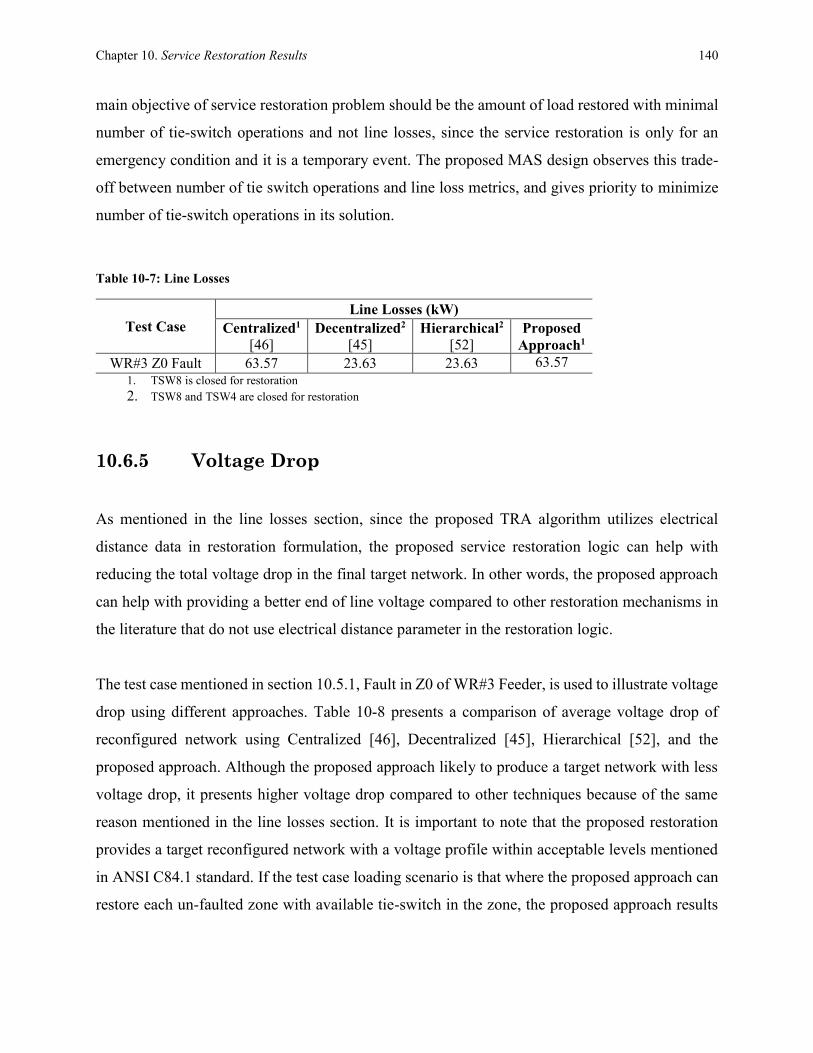
Chapter 10. Service Restoration Results 140
main objective of service restoration problem should be the amount of load restored with minimal
number of tie-switch operations and not line losses, since the service restoration is only for an
emergency condition and it is a temporary event. The proposed MAS design observes this trade-
off between number of tie switch operations and line loss metrics, and gives priority to minimize
number of tie-switch operations in its solution.
Table 10-7: Line Losses
Test Case
Line Losses (kW)
Centralized1
[46] Decentralized2
[45] Hierarchical2
[52] Proposed
Approach1
WR#3 Z0 Fault 63.57 23.63 23.63 63.57
1. TSW8 is closed for restoration
2. TSW8 and TSW4 are closed for restoration
10.6.5 Voltage Drop
As mentioned in the line losses section, since the proposed TRA algorithm utilizes electrical
distance data in restoration formulation, the proposed service restoration logic can help with
reducing the total voltage drop in the final target network. In other words, the proposed approach
can help with providing a better end of line voltage compared to other restoration mechanisms in
the literature that do not use electrical distance parameter in the restoration logic.
The test case mentioned in section 10.5.1, Fault in Z0 of WR#3 Feeder, is used to illustrate voltage
drop using different approaches. Table 10-8 presents a comparison of average voltage drop of
reconfigured network using Centralized [46], Decentralized [45], Hierarchical [52], and the
proposed approach. Although the proposed approach likely to produce a target network with less
voltage drop, it presents higher voltage drop compared to other techniques because of the same
reason mentioned in the line losses section. It is important to note that the proposed restoration
provides a target reconfigured network with a voltage profile within acceptable levels mentioned
in ANSI C84.1 standard. If the test case loading scenario is that where the proposed approach can
restore each un-faulted zone with available tie-switch in the zone, the proposed approach results

Chapter 10. Service Restoration Results 141
in less voltage drop. The proposed MAS design gives priority to minimize number of tie-switch
operations over voltage drop metric as the event is a temporary one.
Table 10-8: Voltage Drop
Test Case
Voltage Drop (%)
Centralized1
[46] Decentralized2
[45] Hierarchical2
[52] Proposed
Approach1
WR#3 Z0 Fault 4.67 2.88 2.88 4.67
1. TSW8 is closed for restoration
2. TSW8 and TSW4 are closed for restoration

142
Chapter 11
Conclusions and Future Work
11.1 Conclusions
In this dissertation, a novel hybrid Multi-Agent System with agent learning capability (Q-learning)
is proposed for electric distribution system automation with DER and microgrids. Also, an
innovative economic model and algorithm is presented for the optimum switch number and
placement problem of DA projects. The main contributions of this work are,
Hybrid Multi-Agent System Design
A new hybrid MAS architecture for distribution automation system is proposed that is
flexible and scalable. The proposed architecture makes use of both Centralized and
Decentralized concepts to make up for the disadvantages of each method and achieve
overall optimal solution. The proposed MAS architecture includes dedicated agents for
distributed generators and microgrids to include those components into the FLIR solution.
The agents can communicate with other agents in the same hierarchical level. However,
the supervisory agents, feeder and substation agents, can exploit peer to peer
communications with the lower level switch agents to reduce number of communications
to speed up the FLIR processes. The decision making happens at the supervisory level, at
the feeder agent or substation agent level, as these agents have the complete view of the
system to achieve the optimal solution.

Chapter 11. Conclusions and Future Work 143
Switch Optimization
An innovative economic model is presented for the optimum switch number and placement
problem of DA projects. The switch optimization is a complex and very important step in
the economic feasibility process of any DA project. The proposed method finds the solution
based on relative reduction in the normalized customer interruption costs. The main
advantage of the proposed approach is that it isolates the impacts of varying switch
investment and customer interruption cost data which is usually based on outdated utility
survey studies. The proposed method is implemented on IEEE 34-bus, 123-bus, and WVSC
test feeders. The mathematical model is developed in Matlab and the results show the
computational robustness and efficacy of the solution. The proposed technique
significantly scales down the search space and simplifies problem complexity that requires
minimal computational effort and time.
Distributed Fault Location and Isolation
Fault location and isolation is the first step of automatic FLIR systems, and faster FLI
means faster service restoration and shorter outage time. Restoration process cannot be
initiated unless the fault location is determined and faulty section is isolated. Therefore, it
is important to locate and isolate the fault as fast as possible and preferably using a non-
centralized approach.
A novel MAS FLI solution is presented for radial electric distribution systems with
different types of DG resources which include synchronous, induction, and inverter-based
resources. Unlike the traditional rotating machines, the fault response of an inverter based
DG depends mostly on its control system rather than its physical parameters. The inverters
are actively current limited due to the low thermal inertia of semiconductor switches, and
thus have a small fault current contribution (1-2 pu) compared to conventional non-inverter
based generators (5-10 pu). Therefore, it is important to correctly account for DG fault
characteristics in the FLI solution. Proposed FLI solution is one of the few available

Chapter 11. Conclusions and Future Work 144
solutions that can locate the fault in electric distribution systems with DG penetrations
without adding additional metering hardware.
The proposed FLI logic is totally distributed in nature that does not rely on centralized
control approaches. An intelligent algorithm for Fault Detection is proposed, which can
identify the faulted zone and also can determine the type of the fault. The sectionalizing
switch agents can determine fault location autonomously based on the proposed Fault
Detection Algorithm using their local data measurements. The fault isolation is achieved
through a coordinated agent communication approach.
The proposed MAS FLI solution is illustrated by performing simulation studies on WVSC
distribution system. A detailed PSCAD model of WR#3 feeder is developed along with
generator models to model a large scale inverter based DG, a synchronous generator, and
an induction generator. The simulation platform is used to test the fault response of various
types of DG resources for various types of faults in the system. The results show efficacy
of the solution and authenticates the proposed MAS based FLI solution that works
efficiently for radial distribution systems with different DG resources and with varying DG
penetration levels.
Hybrid Service Restoration and Reconfiguration
The proposed service restoration approach is based on a hybrid philosophy that utilizes
both central and distributed control methods to make up for the disadvantages of each
method and achieve an overall optimal solution. The proposed service restoration approach
uses the “Tie-Switch Ranking Algorithm” and the “Zone Priority Algorithm” and makes
use of available DG units and microgrids to find the best possible service restoration plan.
The solution is formulated as a combinatorial multi-objective optimization to maximize
amount of load restored with minimal number of tie-switch operations while maximizing
available microgrids in the system.

Chapter 11. Conclusions and Future Work 145
The proposed solution is tested on the real distribution system of WVSC project. The
system include two substations and total of eight distribution feeders. The actual
distribution network is simulated in CYME® and Matlab®/Simpower® whereas the MAS
and its communications are simulated using Matlab® S-functions. The simulation results
show promising advantages of using the proposed MAS solution for service restoration.
A key set of performance metrics are identified in order to evaluate performance of the
proposed MAS service restoration solution in terms of solution quality and speed. The
proposed MAS service restoration solution is compared with other solution methods in
literature such as Centralized [46], Decentralized [45], and Hierarchical [52], as they
present different control approach and solution architecture for the same problem. The
evaluation revealed that the proposed approach results in less number of overall agent
communications, hence faster service restoration, less number of tie-switch operations, and
more number of un-faulted zone restored compared to the other methods. However, the
proposed approach compromises on line losses and voltage drop metrics to meet other
needed objectives of the service restoration.
Reinforcement Agent Learning
Although the agents in MAS can be programmed with behaviors designed in advance, it is
also necessary that they learn new behaviors online from their experiences, such that the
performance of the agents and MAS gradually improves. In this dissertation, a modified
reinforcement learning based on Q-learning is introduced to help agents in their decision
making process. Although agents have the learning capability, they need to take actions to
learn from them. In a real world power system fault events do not happen frequently and
therefore it takes a long time for agents to gain knowledge about different scenarios. One
possible solution to help agents learn faster is initializing agents’ knowledge by simulating
different possible scenarios in a software environment.

Chapter 11. Conclusions and Future Work 146
Using the learning technology, agents in EDS will be expert decision makers over time and
can make more accurate and comprehensive decisions for a self-healing distribution
system.
11.2 Future Work
While this dissertation has discussed the design of a MAS for electric distribution system
automation, many opportunities for extending the scope of this dissertation remain. The following
main items can be suggested as future work:
1. MAS application for Microgrids
Although this dissertation has presented a MAS application for distribution automation to
solve FLIR problems, there are many areas of power system where the MAS can be a key
technology. MAS can offer modular, flexible, and integrated solutions for many complex
issues of power systems. Microgrid is one such area, where MAS can provide distributed
and autonomous solutions for real-time control and management.
The Smart Grid evolution is transforming the traditional distribution grids from passive to
active networks due to the integration of microgrids and DER. Microgrids are among the
most promising tools of modern distribution networks due to their versatility, which is
demonstrated by the ability to simultaneously deliver enhanced reliability, security, energy
and cost efficiency, as well as environmental benefits. The proliferation of microgrids and
DER is making real-time control and system operations of traditional distribution grid more
complicated. Therefore, smart control and energy management systems that are different
from those commonly used in the past are necessary for efficient operation of modern
power systems. The distributed nature and potential for modeling autonomous decision
making entities in solving complex problems motivates the use of MAS for the control and
management of microgrids. Proposed MAS has the autonomous decision making agents
that can be modified for real-time control and management of a microgrid. Also, the MAS
design can be extended for FLI within microgrids.

Chapter 11. Conclusions and Future Work 147
2. Switch optimization economic model
Proposed economic model finds optimal number and location of automated sectionalizing
switches based on relative reduction in the normalized customer interruption costs. The
proposed model can be extended to form a comprehensive DA cost benefit frame work that
can encompass all DA costs and benefits. The comprehensive model can include reliability
improvements, in terms of SAIDI, CAIDI, and SAIFI indices, due to different switching
technologies such as automated load break switches, reclosers, and sectionalizers.
The proposed method can be easily modified to accommodate other switching technologies
such as reclosers and circuit breakers with various automation levels. Proposed approach
cab be extended to include certain operational considerations such as back-feed capability
without violating thermal loading and voltage constraints to arrive at the solution. Inclusion
of a distribution load flow to find the optimal number and placement of switches can be
the immediate future work.
3. Hardware implementation and testing
Although proposed MAS solution for DA has been tested through simulation studies and
the results are discussed, its application in a real world implementation can further prove
the concept and provide additional insight into potential issues. There are various issues
such as control and communication between agents and power system which are not always
taken into consideration in the simulation studies. The proposed MAS DA solution is
designed to be implemented on a real world distribution network as part of the DOE
demonstration project, WVSC. The project ended as a design-only project, and the MAS
solutions that were designed never got an opportunity to be fully implemented in the real
distribution field. Development of a test system platform capable of emulating a present
day power system and MAS will help in dealing with these challenges.

148
Bibliography
[1] The U.S Department of Energy (DOE), [Online]. Available:
http://energy.gov/oe/services/technology-development/smart-grid.
[2] "A vision for the modern grid," National Energy Technology Laboratory (NETL),
[Online]. Available: http://www.netl.doe.gov/smartgrid/.
[3] L. Xu, M. Y. Chow, J. Timmis and L. S. Taylor, "Power Distribution Outage Cause
Identification With Imbalanced Data Using Artificial Immune Recognition System
(AIRS) Algorithm," IEEE Transactions on Power Systems, vol. 22, no. 1, pp. 198-204,
February 2007.
[4] D. M. Staszesky, D. Craig and C. Befus, "Advanced feeder automation is here," IEEE
Power and Energy Magazine, pp. 56-63, Sept.-Oct. 2005.
[5] [Online]. Available: http://smartgrid.ieee.org/newsletters/april-2014/distribution-
automation-and-the-self-healing-network.
[6] S. Chouhan, H. Wan, H. J. Lai, A. Feliachi and M. A. Choudhry, "Intelligent
reconfiguration of smart distribution network using multi-agent technology," in 2009
IEEE Power & Energy Society General Meeting, Calgary, AB, 2009.
[7] S. Chouhan, J. Ghorbani, H. Inan, A. Feliachi and M. A. Choudhry, "Smart MAS
restoration for distribution system with Microgrids," in 2013 IEEE Power & Energy
Society General Meeting, Vancouver, BC, 2013.
[8] S. Chouhan, F. D. Mohammadi, A. Feliachi, J. M. Solanki and M. A. Choudhry, "Hybrid
MAS Fault Location, Isolation, and Restoration for smart distribution system with
Microgrids," in 2016 IEEE Power and Energy Society General Meeting (PESGM),
Boston, MA, 2016.

Bibliography 149
[9] S. Chouhan, H. Inan and A. Feliachi, "Optimal number and placement of automated
sectionalizing switches for smart grid Distribution Automation," in 2016 IEEE Power
and Energy Society General Meeting (PESGM), Boston, MA, 2016.
[10] S. Chouhan, H. Inan, "Automated Sectionalizing Switch Optimization for Smart Grid
Distribution Automation," in CIGRE US National Committee Grid of the Future
Symposium, Philadelphia, PA, 2016.
[11] J. Ghorbani, S. Chouhan, M. A. Choudhry, and A. Feliachi, "Hybrid multi agent
approach for power distribution system restoration," in 2013 IEEE Energytech,
Cleveland, OH, 2013.
[12] M. Baran, A. Padmanabhan, S. Chouhan, X. Yuan, J. Smith and H. Mayfield, "A model
based fault locating method for distribution systems," in 2014 IEEE PES General
Meeting | Conference & Exposition, National Harbor, MD, 2014.
[13] G. Weiss, Multi-agent Systems: A Modern Approach to Distributed Artificial
Intelligence, The MIT Press, 2000.
[14] D. A. Cartes and S. K. Srivastava, "Agent Applications and their Future in the Power
Industry," in 2007 IEEE Power Engineering Society General Meeting, Tampa, FL, 2007.
[15] Zhong Zhang, J. D. McCalley, V. Vishwanathan and V. Honavar, "Multiagent system
solutions for distributed computing, communications, and data integration needs in the
power industry," in IEEE Power Engineering Society General Meeting, 2004.
[16] G. Levitin, S. Mazal-Tov, and D. Elmakis, "Genetic algorithm for optimal sectionalizing
in radial distribution systems with alternative supply," Electr. Power Syst. Res., vol. 35,
no. 3, pp. 149-155, 1995.
[17] R. Billinton and S. Jonnavithula, "Optimal switching device placement in radial
distribution systems," IEEE Transactions on Power Delivery, vol. 11, no. 3, pp. 1646-
1651, July 1996.
[18] P. M. S. Carvalho, L. A. F. M. Ferreira and A. J. C. da Silva, "A decomposition approach
to optimal remote controlled switch allocation in distribution systems," IEEE
Transactions on Power Delivery, vol. 20, no. 2, pp. 1031-1036, April 2005.
[19] Chao-Shun Chen, Chia-Hung Lin, Hui-Jen Chuang, Chung-Sheng Li, Ming-Yang
Huang and Chia-Wen Huang, "Optimal placement of line switches for distribution

Bibliography 150
automation systems using immune algorithm," IEEE Transactions on Power Systems,
vol. 21, no. 3, pp. 1209-1217, August 2006.
[20] L. G. W. da Silva, R.A.F. Pereira, J.R. Abbad, and J.R.S. Mantovani, "Optimised
placement of control and protective devices in electric distribution systems through
reactive tabu search algorithm," Electr. Power Syst. Res., vol. 78, no. 3, p. 372–381,
2008.
[21] A Moradi, M. Fotuhi-Firuzabad, and M. Rashidi-Nejad, "A reliability cost/worth
approach to determine optimum switching placement in distribution systems," in Proc.
IEEE Power Eng. Soc. Asia Pacific Transmission Distribution Conf. Exhib, 2005.
[22] A. Moradi and M. F. Firuzabad, "Optimal switch placement in distribution systems using
trinary particle swarm optimization algorithm," IEEE Trans. Power Del., vol. 23, no. 1,
p. 271–279, Jan. 2008.
[23] H. Falaghi, M. R. Haghifam and C. Singh, "Ant Colony Optimization-Based Method for
Placement of Sectionalizing Switches in Distribution Networks Using a Fuzzy
Multiobjective Approach," IEEE Transactions on Power Delivery, vol. 24, no. 1, pp.
268-276, Jan. 2009.
[24] M. Kezunovic, "Smart Fault Location for Smart Grids," IEEE Transactions on Smart
Grid, vol. 2, no. 1, pp. 11-22, March 2011.
[25] J. Mora-Florez, J. Melendez, and G. Carrillo-Caicedo, "Comparison of impedance based
fault location methods for power distribution systems," Elect. Power Syst. Res., vol. 78,
p. 657–666, 2008.
[26] J. Izykowski M. M. Saha and E. Rosolowski, Fault Location on Power Networks, 2010,
Springer-Verlag, 2010.
[27] N. Karnik, S. Das, S. Kulkarni and S. Santoso, "Effect of load current on fault location
estimates of impedance-based methods," in 2011 IEEE Power and Energy Society
General Meeting, San Diego, CA, 2011.
[28] J. Ghorbani, M. Choudhry, and A. Feliachi, "Fault location and isolation using multi
agent systems in power distribution systems with distributed generation sources," in
Innovative Smart Grid Technologies (ISGT), 2013 IEEE PES, 2013.

Bibliography 151
[29] G. C. Lampley, "Fault detection and location on electrical distribution system," in proc.
of IEEE Rural Electric Power Conference, 2002.
[30] P. Verho M. M. Saha, R. Das and D. Novosel, "Review of Fault Location Techniques
for Distribution Systems,” proc. of Int. Conf on Power Systems and Communications
Infrastructures," in proc. of Int. Conf on Power Systems and Communications
Infrastructures, Beijing, 2002.
[31] D. Thukaram, H. P. Khincha and H. P. Vijaynarasimha, "Artificial neural network and
support vector Machine approach for locating faults in radial distribution systems,"
IEEE Transactions on Power Delivery, vol. 20, no. 2, pp. 710-721, April 2005.
[32] N. Karnik S. Das, S. Kulkarni and S. Santoso, "Distribution fault location using short-
circuit fault current profile approach," in proc. of IEE PES GM, 2011.
[33] M. Michalik, W. Rebizant, M. Lukowicz, Seung-Jae Lee and Sang-Hee Kang, "High-
impedance fault detection in distribution networks with use of wavelet-based
algorithm," IEEE Transactions on Power Delivery, vol. 21, no. 4, pp. 1793-1802, Oct.
2006.
[34] J. J. Mora, G. Carrillo and L. Perez, "Fault Location in Power Distribution Systems using
ANFIS Nets and Current Patterns," in 2006 IEEE/PES Transmission & Distribution
Conference and Exposition: Latin America, Caracas, 2006.
[35] J. Mora-Florez, V. Barrera-Nunez and G. Carrillo-Caicedo, "Fault Location in Power
Distribution Systems Using a Learning Algorithm for Multivariable Data Analysis,"
IEEE Transactions on Power Delivery, vol. 22, no. 3, pp. 1715-1721, July 2007.
[36] A.L. Morelato and A. Monticelli, "Heuristic search approach to distribution system
restoration," IEEE Transactions on Power Delivery, vol. 4, no. 4, pp. 2235-2241, Oct.
1989.
[37] C. C. Liu, S. J. Lee and S. S. Venkata, "An expert system operational aid for restoration
and loss reduction of distribution systems," IEEE Transactions on Power Systems, vol.
3, no. 2, pp. 619-626, 1988.
[38] W. Isamu and N. Makoto, "A genetic algorithm for optimizing switching sequence of
service restoration in distribution systems," in Proc. Congr. Evolutionary Computation,
2004.

Bibliography 152
[39] Y. Fukuyama, "Reactive Tabu Search for distribution load transfer operation," in Proc.
IEEE Power Eng. Soc. Winter Meeting, 2000.
[40] K. H. Jung, H. Kim, and Y.Ko, "Network reconfiguration algorithm for automated
distribution systems based on artificial intelligence," IEEE Trans. Power Del., vol. 8,
no. 4, p. 1933–1941, Oct. 1993.
[41] S. Das, S. Bose, S. Pal, N. N. Schulz, C. M. Scoglio and B. Natarajan, "Dynamic
reconfiguration of shipboard power systems using reinforcement learning," IEEE
Transactions on Power Systems, vol. 28, no. 2, pp. 669-676, May 2013.
[42] R. Perez-Guerrero, G. T. Heydt, N. J. Jack, B. K. Keel and A. R. Castelhano, "Optimal
Restoration of Distribution Systems Using Dynamic Programming," IEEE Transactions
on Power Delivery, vol. 23, no. 3, pp. 1589-1596, July 2008.
[43] T. Nagata, Y. Tao, K. Kimura, H. Sasaki, and H. Fujita, "A multi-agent approach to
distribution system restoration," in Circuits and Systems, 2004. MWSCAS '04. The 2004
47th Midwest Symposium, 2004.
[44] Fabio Luigi Bellifemine, Giovanni Caire, Dominic Greenwood, Developing Multi-
Agent Systems with JADE, Wiley, 2007.
[45] J. M. Solanki, S. Khushalani and N. N. Schulz, "A Multi-Agent Solution to Distribution
Systems Restoration," IEEE Transactions on Power Systems, vol. 22, no. 3, pp. 1026-
1034, 2007.
[46] T. Nagata and H. Sasaki, "A multi-agent approach to power system restoration," IEEE
Transactions on Power Systems, vol. 17, no. 2, pp. 457-462, May 2002.
[47] T. Nagata, N. Iba, Y. Tao and H. Sasaki, "A new power system restoration framework
by means of multi-agent approach," in IEEE/PES Transmission and Distribution
Conference and Exhibition, 2002.
[48] T. Nagata, Y. Tao, Y. Tahara, T. Aoyama, H. Fujita and M. Koaizawa, "Development
of bulk power system restoration simulator by means of multi-agent approach," in
Circuits and Systems, 2004. MWSCAS '04. The 2004 47th Midwest Symposium on, 2004.
[49] Dong Liu, Yunping Chen, Guang Shen and Youping Fan, "A Multi-Agent Based
Approach for Modeling and Simulation of Bulk Power System Restoration," in 2005

Bibliography 153
IEEE/PES Transmission & Distribution Conference & Exposition: Asia and Pacific,
Dalian, 2005.
[50] Belkacemi, Rabie, and Ali Feliachi, "Multi-agent design for power distribution system
reconfiguration based on the artificial immune system algorithm," in Circuits and
Systems (ISCAS), Proceedings of 2010 IEEE International Symposium on, 2010.
[51] Belkacemi, Rabie, Ali Feliachi, M. A. Choudhry, and J. E. Saymansky, "Multi-Agent
systems hardware development and deployment for smart grid control applications," in
Power and Energy Society General Meeting, 2011.
[52] M. J. Ghorbani, M. A. Choudhry and A. Feliachi, "A Multiagent Design for Power
Distribution Systems Automation," IEEE Transactions on Smart Grid,, vol. 7, no. 1, pp.
329-339, Jan 2016.
[53] P. Stone and M. Velos, "Multiagent systems: a survey from the machine learning
perspective," Autonomous Robots, vol. 8, no. 3, pp. 345-383, 2000.
[54] R. Sutton and A. Barto, Reinforcement Learning: An Introduction, The MIT Press, 1998.
[55] K. S. Narendra and M. A. L. Thathachar, Learnng Automata: An Introduction, Prentice
Hall, 1989.
[56] C. J. C. H. Watkins, and P. Dayan, "Q-learning," Machine Learning, vol. 8, no. 3, pp.
279-292, May 1992.
[57] D. Ye, M. Zhang and D. Sutanto, "A Hybrid Multiagent Framework With Q-Learning
for Power Grid Systems Restoration," IEEE Transactions on Power Systems, vol. 26,
no. 4, pp. 2434-2441, Nov. 2011.
[58] J. Jung, Chen-Ching Liu, S. L. Tanimoto and V. Vittal, "Adaptation in load shedding
under vulnerable operating conditions," IEEE Transactions on Power Systems, vol. 17,
no. 4, pp. 1199-1205, Nov. 2002.
[59] "IntelliTeam SG Automatic Restoration System," S&C Electric Company, [Online].
Available: http://www.sandc.com/products/automation-control/.
[60] M. Wooldridge, N. R. Jennings, "Intelligent agents: Theory and Practice," The
Knowledge Engineering Review, vol. 10, no. 2, p. 115 – 152, 1995.

Bibliography 154
[61] S. Russell and P.Norvig, Artificial Intelligence: A modern approach, Printice-Hall,
1995.
[62] Donald A. Waterman; Frederick Hayes-Roth; Douglas B. Lentat, Building Expert
Systems, Reading, MA : Addison-Wesley Publishing Co, 1983.
[63] P.Jackson, Introduction to Expert Systems, Reading, M.A: Addison-Wesley, 1986.
[64] John R Searle, Speech Acts: An essay in the philosophy of Language, Cambridge U.
Press, 1970.
[65] "The Foundation for Physical Intelligent Agents," [Online]. Available:
http://www.fipa.org.
[66] "FIPA 97 specifications, version 2.0, ACL," [Online]. Available: http://www.fipa.org.
[67] C. S. Chen, C. H. Lin, H. J. Chuang, C. S. Li, M. Y. Huang, and C. W. Huang, "Optimal
placement of line switches for distribution automation systems using immune
algorithm," IEEE Trans. Power Syst., vol. 21, no. 3, p. 1209–1217, 2006.
[68] W. H. Kersting, "Radial Distribution Test Feeders," IEEE Trans. On Power Systems,
vol. 6, no. 3, Aug 1991.
[69] C.A. Plet, M. Graovac, R. Iravani, T.C. Green, "Fault response of grid-connected
inverter dominated networks," in IEEE Power and Energy Society General Meeting,
2010.
[70] J. Keller, B. Kroposki, "Understanding Fault Characteristics of Inverter-Based
Distributed Energy Resources," Natl.Renew. Energy Lab, 2010.
[71] M. Baran, I. El-Markaby, "Fault analysis on distribution feeders with distributed
generators," IEEE Trans. Power Syst., vol. 20, no. 4, p. 1757–1764, 2005.
[72] B. Kroposki, Optimization of Distributed and Renewable Energy Penetration in Electric
Power Distribution Systems, Thesis Submitted to CSM, Golden, Colorado, 2008.
[73] IEEE Std 141-1993 Red Book – Electric Power Distribution for Industrial Plants, IEEE,
1993.
Bibliography 155
[74] IEEE. IEEE 1547.2-2008. Standard for Interconnecting Distributed Resources with
Electric Power Systems, IEEE, 2008.
[75] C. A. Plet, T. C. Green, "Fault response of inverter interfaced distributed generators in
grid-connected applications," Elect. Power Syst. Res., vol. 106, pp. 21-28, Jan. 2014.
[76] R. Lasseter, "Dynamic models for micro-turbines & fuel cells," in Proc. IEEE Power
Eng. Soc. Summer Meeting, 2001.
[77] M. Baran and I. El-Markabi, "An EMTP based simulator for distribution systems with
distributed generation," in Proc. Power System Conf. Impact Distributed Generation,
Clemson, SC, 2002.
[78] IEEE Recommended Practice for Utility Interface of Photovoltaic (PV) Systems, IEEE
std. 929-2000, IEEE, 2000.
[79] T. S. Basso, and R. DeBlasio, "IEEE 1547 series of standards: interconnection issues,"
IEEE Transactions on Power Electronics, vol. 19, no. 5, p. 1159 – 1162, 2004.
[80] IEEE Standard for Electrical Power System Device Function Numbers, Acronyms and
Contact Designation, IEEE Std. C37.2, IEEE, 2008.
[81] K. N. Miu, Hsiao-Dong Chiang, Bentao Yuan and G. Darling, "Fast service restoration
for large-scale distribution systems with priority customers and constraints," IEEE
Transactions on Power Systems, vol. 13, no. 3, pp. 789-795, 1998.
[82] W. H . Kersting, Distribution system modeling and analysis, 2 ed., Boca Raton, Florida:
Taylor & Francis Group, 2006, p. 45.
[83] L. Busoniu, R. Babuska, and B. De Schutter, "A comprehensive survey of multiagent
reinforcement learning," IEEE Trans. Systems, Man, and Cybernetics, Part C:
Applications and Reviews, vol. 38, no. 2, pp. 156-172, 2008.