A Monthly Journal of Computer Science and Information ... · Cost 231 extension to Hata Model A...

NWALOZIE GERALD.C et al, International Journal of Computer Science and Mobile Computing, Vol.3 Issue.2, February- 2014, pg. 267-281

© 2014, IJCSMC All Rights Reserved 267

Available Online at www.ijcsmc.com

International Journal of Computer Science and Mobile Computing

A Monthly Journal of Computer Science and Information Technology

ISSN 2320–088X

IJCSMC, Vol. 3, Issue. 2, February 2014, pg.267 – 281

RESEARCH ARTICLE

PATH LOSS PREDICTION FOR GSM MOBILE NETWORKS FOR URBAN

REGION OF ABA, SOUTH-EAST NIGERIA

NWALOZIE GERALD .C1, UFOAROH S.U2, EZEAGWU C.O3, EJIOFOR A.C4 1, 2, 3 Department of Electronic and Computer Engineering, Nnamdi Azikiwe University Awka,

Anambra State Nigeria 4 Department of Industrial Production Engineering, Nnamdi Azikiwe University Awka,

Anambra State Nigeria

ABSTRACT

Propagation path loss greatly impact on the quality of service of a mobile communication system. To establish any mobile communication system, the basic task is to foresee the coverage of the proposed system in general, and the accurate determination of the propagation path loss leads to development of efficient design and operation of quality networks. Many such different approaches have been developed, over the past, to predict coverage using what are known as propagation models. However, such models, no matter how accurate, will result in co-channel interference and wastage of power when they are used in environments for which they were not developed. So, the best bet is to perform site-specific measurements. This paper presents a measurement-based path loss model, from experimental data collected in Aba urban, South-East Nigeria. Received Signal Strength (RSS) measurements were gathered in Aba from GlobalCom Limited (GLO) Network operating at 900MHz. The results of the measurements were used to develop path loss model for the urban environment, the result shows that the path loss for the measurement environment increases by 3.10dB per decade.

KEYWORDS: Base Station, Path Loss, Propagation, Model, GSM.



I. INTRODUCTION

Radio propagation is essential for emerging technologies with appropriate deployment and measurement strategies for any wireless network. It is heavily site specific and can vary significantly depending on terrain frequency of operation, velocity of mobile terminal, antenna heights etc. accurate characterization of radio channel through key parameters and a mathematical model is important for predicting signal coverage, achievable data rates, specific performance attributes of alternative signaling and reception schemes [1]. Planning is the key before implementing designs, and also setting up of wireless communication systems. Precise propagation characteristics of the situation should be known. Usually propagation provides two types of data, corresponding to the large-scale path loss and small-scale statistics pertaining to fading issue. Information regarding path-loss is very pivotal, for knowing the coverage of a base-station (BS) and in optimizing it. The statistics provided by the small-scale parameters pertain only to local field variations. Also in turn this helps to improvise receiver (Rx) design structure and counter the multipath fading. Without propagation predictions, these parameter estimations can only be obtained by field measurements which are time consuming and expensive.

Path loss is the reduction in power of an electromagnetic wave as it propagates through space. It is a major component in analysis and design of link budget of a communication system [2]. It depends on frequency, antenna height, receive terminal location relative to obstacles and reflectors, and link distance, among many other factors. Propagation path loss models prediction plays an important role in the design of cellular systems to specify key system parameters such as transmission power, frequency, antenna heights etc.

GSM (Global System for Mobile Communications) comes under wireless communication, which depends on the propagation of waves in the free space and providing transmission of data [3].It extends service by providing mobility for users, which fulfills the subscribers demand at any terrain covered by wireless network. When we consider the earlier historical legacy, the growth in mobile communications field has now become less. Here, the paramount factor was to serve for high quality and high capacity networks. Estimated coverage precisely has become very pivotal. Therefore to accomplish far more accurate design, coverage of modern cellular networks and received signal strength measurements will be considered as source of data, in order to provide reliable and efficient coverage locality. This research aims to improve the quality of wireless services in Aba urban environment in the South-East region of Nigeria by carrying out site specific measurements and developing an acceptable Path loss model for the region.

In Section II, some existing Pathloss models widely in use are presented. Section II, some related literatures were reviewed. Section IV describes the method of data collection deployed. Section V presents data analysis and results. In Section VI we compared the measured results with results from existing models and propose possible adjustments to Hata (urban) model for improved accuracy of its use within Aba urban.

II. PROPAGATION PATH LOSS MODELS

These models can be broadly categorized into three types; empirical, deterministic and stochastic. Empirical models are those based on observations and measurements alone. The deterministic models make use of the laws governing electromagnetic wave propagation to determine the received signal power



at a particular location. Deterministic models often require a complete 3-D map of the propagation environment. Stochastic models, on the other hand, model the environment as a series of random variables. Macro cells are generally large, providing a coverage range in kilometers and used for outdoor communication [4]. Several empirical path loss models have been determined for macro cells. Among numerous propagation models, the following are the most significant ones, providing the foundation of mobile communication services. The models include;

Okumura’s Model

The Okumura model is an empirical model based on extensive measurements made in Japan at several frequencies in the range from 150-1920MHz (it is also extrapolated up to 3000MHz). Okumura’s model is basically developed for macrocells with cell diameters from 1 to 100km. The heights of the BS antenna are between 30-1000m. The Okumura model takes into account some of the propagation parameter such as the type of environment and the terrain irregularity. The basic prediction formula is as follows:

)1()()(),()( , nGcorrectiohreGhteGdfALfreedBLmean um

Where, Lmean (dB) is the median value of the propagation path loss, Lfree is the free – space path loss, and can be calculated using:

)2(])4/(log[10)( 22 dGtGrdBL

Am,u is the median attenuation value relative to free space in an urban, )(hteG and )(hreG are the height

gain factors of BS and mobile antennas, and nGcorrectio is determined by looking up curves derived

from measurements. )(hteG and )(hreG are calculated using simple formulas.

Terrain information can be qualitatively included in the Okumura model. For example, the propagation environments are categorized as open area, quasi-open area, and suburban area. Other information such as terrain modulation height and average slope of terrain can also be included. Okumura derived empirical

formulas for )(hteG and )(hreG as:

)3(10030),200/log(20)( mhtemhtehteG

)5(103),3/log(20)4(3),3/log(10)(

mhremhremhrehrehreG

Okumura’s model has a 10-14db empirical standard deviation between the path loss predicted by the model and the path loss associated with one of the measurements used to develop the model. Okumura’s model is wholly based on measured data and doesn’t provide any analytical explanation. The major disadvantage with the model is its slow response to rapid changes in the terrain; therefore the model is fairly good in urban and suburban areas, but not good in rural areas [5].



Hata Model

The Hata model [6] is an empirical formulation of the graphical path loss data provided by Okumura and is valid over roughly the same range of frequencies, 150-1500MHz. This empirical model simplifies calculation of path loss since it is a closed form formula and is not based on empirical curves for the different parameters.

The standard formula for median path loss in urban areas under the Hata model is:

)6(log))log(55.69.44()()log(82.13)log(16.2655.69)(

dhtehreahtefcdBLurban

Where )(hrea is a correction factor for the mobile antenna height based on the size of the coverage area. For small to medium sized cities, this factor is given by:

)7(8.0)log(56.1()7.0)log(1.1()( fchrefchrea

and for larger cities at frequencies ,MHzfc 300

)8(97.4))75.11(log(2.3)( 2 dBhrhrea

Corrections to the urban model are made for suburban and rural propagation, so that these models are:

)10()log(33.18)][log(78.4)()()9(4.5)]28/[log(2)()(

2

2

KfcfcdBLurbandBLruralfcdBLurbandBLsuburban

Where k ranges from 35.94 (country side) to 40.94(desert). The Hata model well-approximates the Okumura model for distances d>1km. Thus, it is a good model for first generation cellular systems, but does not model propagation well in current cellular systems with smaller cell sizes and higher frequencies. Indoor environments are also not captured with the Hata model.

Cost 231 extension to Hata Model

A model that is widely used for predicting path loss in mobile wireless system is the COST-231 Hata model [7]. The cost-231 Hata model is designed to be used in the frequency band from 500MHz to 2000MHz. it also contains corrections for urban, suburban and rural (flat) environments. Although its frequency range is outside that of the measurements, its simplicity and the availability of correction factors have made it widely used for path loss prediction at this frequency band. The basic equation for path loss in dB is:

)11(log))log(55.69.44()log(82.13)log(9.333.46

Cmdhb

ahmhbfPL

Where, f is the frequency in MHz, d is the distance between AP and CPE antennas in KM, and hb is the AP antenna height above ground level in meters. The parameter Cm is defined as OdB for suburban or



open environments and 3dB for urban environments. The parameter ahm is defined for urban environments as:

)12(400,97.4))75.11(log(20.3 2 MHzfhrahm

For suburban or rural (flat) environments,

)13()8.0log56.1()7.0log1.1( fhrfahm

Where, hr is the CPE antenna height above ground level. From (11) and (13), the path loss exponent of the predictions made by COST-231 Hata mode is given by:

)14(10/))log(55.69.44(cos hbn t

To evaluate the applicability of the cost-231 model for the 3.5GHz band, the model predictions are compared against measurements for three different environments, namely, rural (flat), suburban and urban.

Free Space Propagation Model

In free space, the wave is not reflected or absorbed. Ideal propagation implies equal radiation in all directions from the radiating source and propagation to an infinite distance with no degradation. Spreading the power over greater areas causes attenuation. Calculating the power flux is given below:

24 dPtPd / ----------------- (15)

Where;

Pt is known as transmitted power (W/m2) and Pd is the power at a distance d from antenna. If the radiating element is generating a fixed power and this power is spread over an ever-expanding sphere, the energy will be spread more thinly as the sphere expands. If a receiver antenna is placed at the point of the power flux density as given above, the power received by the antenna can be calculated. The formula for calculating the effective antenna aperture is given by:

)16(4/2 Ae

Where; Ae = Effective area of an isotropic antenna.

λ= wavelength of received signal.

The received power at the distance d is therefore given as,

)17()4/(Pr 22 dPtxPdxAe

That is to say that the amount of power received by the antenna at the required distance d, depends on the effective aperture of the antenna and the power flux density at the receiving element.



The path loss ( Lp ) is given by;

Lp= power transmitted (Pt) – power received (Pr),

From equation (17) we have ;

224 /)(Pr/ dPt

)18()log(20)log(20)4log(20)( ddBLp

Given that the wavelength , is km and the frequency f, is in MHz, i.e,

)19(/3.0 f

Rationalizing equation (19) gives the generic free space path loss formula which is given as:

)20()log(20)log(205.32)( fddBLPfs

It is assumed that both transmitting and receiving antennas are isotropic, i.e, 1 GrGt

Log-Normal Shadowing Model

Basically, in a terrestrial wireless environment, signal propagation is characterized by such factors as path loss, shadowing and fading. Path loss has been defined as the attenuation effect on the signal as it propagates from the transmitter to the receiver. When the received signal strength gradually varies around its average value, this characteristic is called shadowing. On the other hand, fading describes the rapid variation in the received signal strength due to multi-path propagation.

A simple power law path loss model [8] was chosen for predicting the distance of reliable communication between two mobiles. A modified power law path loss model is give as:

)21()/log(10)()( dodndoLpdiLp

where

n = ( ) ( )

( ) (22)

where xσ is a Zero-Mean Gaussian distributed random variable (in dB) with standard deviation σ (in dB). Using linear regression analysis, the path loss exponent, n, can be determined by minimizing (in a mean square error, sense) the difference between measured and predicted values of equation (22) to yield:

n = ∑ [ ( ) ( )]

∑ ( ) (23)



The standard deviation, σ is equally minimized using the formula:

σ = ∑ ( ) (24)

where, Pm = Measured Path Loss

Pr = Predicted Path Loss

N = Number of measured data points

Received Power, Pr in (dBm), at any distance D from the Transmitter, with Transmit Power, Pt in (dBm) is given by:

Pr (dBm) = Pt (dBm) – Lp (dB) (25)

Pr can be evaluated from measured data for any distance (di), using the formula:

Pr (dB) = 10Log Pr (do) (26)

III. RELATED WORKS

In [9], Z. Nadir et al investigated the characteristics of radio propagation, by measurement, at the small town of rural area in Purwokerto Central Java Indonesia. His results were used to evaluate the accuracy of Okumura Hata and Lee prediction models and to determine the necessary adjustments to these models in order to improve their accuracies. He radiated a 20dBm signal at 1467MHz by an omni directional antenna with 5.2dB gain. His propagation measurements showed that the received signal strength decreases with distance at the rate of 2.34dB, while its mean values fall between 10 and 15dB below free space prediction with standard deviation of 6.5dB. Comparing his propagation measurements with Okumura- Hata and Lee prediction models for open area classifications, he discovered that they were in agreement for area coverage of 3 to 10Km. Also, Okumura-Hata and Lee models gave less path loss prediction for smaller coverage area but propose higher values for larger distances.

In [10], Z.Nadir, et al, on examining the applicability of Okumura-Hata model in Oman in the GSM frequency band, adapted a propagation model for Salalah (Oman). The authors accomplished their modification by investigating the variation in path loss between the measured and predicted values according to Okumura-Hata propagation model for a cell in Salalah city and then found the missing experimental data with spline interpolation. Then, they modified the Okumura-Hata model according to the results obtained in their investigations. Furthermore, they verified their modified model by applying it for other cells. They calculated the mean square error (MSE) between the measured path loss values and those predicted on basis of Okumura-Hata model for an open area. The MSE was about 6dB, which is an acceptable value for the signal prediction. That error was minimized by subtracting the calculated MSE (15.31dB) from the original equation of open area for Okumura –Hata model. Hence, they derived a path loss equation for Salalah city.



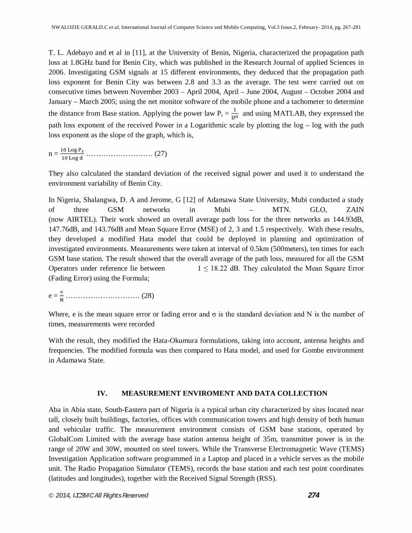
T. L. Adebayo and et al in [11], at the University of Benin, Nigeria, characterized the propagation path loss at 1.8GHz band for Benin City, which was published in the Research Journal of applied Sciences in 2006. Investigating GSM signals at 15 different environments, they deduced that the propagation path loss exponent for Benin City was between 2.8 and 3.3 as the average. The test were carried out on consecutive times between November 2003 – April 2004, April – June 2004, August – October 2004 and January – March 2005; using the net monitor software of the mobile phone and a tachometer to determine the distance from Base station. Applying the power law Pr = and using MATLAB, they expressed the path loss exponent of the received Power in a Logarithmic scale by plotting the log – log with the path loss exponent as the slope of the graph, which is,

n =

……………………… (27)

They also calculated the standard deviation of the received signal power and used it to understand the environment variability of Benin City.

In Nigeria, Shalangwa, D. A and Jerome, G [12] of Adamawa State University, Mubi conducted a study of three GSM networks in Mubi – MTN. GLO, ZAIN (now AIRTEL). Their work showed an overall average path loss for the three networks as 144.93dB, 147.76dB, and 143.76dB and Mean Square Error (MSE) of 2, 3 and 1.5 respectively. With these results, they developed a modified Hata model that could be deployed in planning and optimization of investigated environments. Measurements were taken at interval of 0.5km (500meters), ten times for each GSM base station. The result showed that the overall average of the path loss, measured for all the GSM Operators under reference lie between 1 ≤ 18.22 dB. They calculated the Mean Square Error (Fading Error) using the Formula;

e = σ ………………………… (28)

Where, e is the mean square error or fading error and σ is the standard deviation and N is the number of times, measurements were recorded

With the result, they modified the Hata-Okumura formulations, taking into account, antenna heights and frequencies. The modified formula was then compared to Hata model, and used for Gombe environment in Adamawa State.

IV. MEASUREMENT ENVIROMENT AND DATA COLLECTION

Aba in Abia state, South-Eastern part of Nigeria is a typical urban city characterized by sites located near tall, closely built buildings, factories, offices with communication towers and high density of both human and vehicular traffic. The measurement environment consists of GSM base stations, operated by GlobalCom Limited with the average base station antenna height of 35m, transmitter power is in the range of 20W and 30W, mounted on steel towers. While the Transverse Electromagnetic Wave (TEMS) Investigation Application software programmed in a Laptop and placed in a vehicle serves as the mobile unit. The Radio Propagation Simulator (TEMS), records the base station and each test point coordinates (latitudes and longitudes), together with the Received Signal Strength (RSS).



The test van drove in the direction of one antenna sector, though there were overlaps from two sectors at some point. At such points, their averages were computed and used as the received power. The areas tested include, Ikot-Ekpene, Aba-owerri Road, Ngwa Road and Eziama, data from sites in these areas were analyzed. To ensure wider and acceptable applicability of the result, data was collected over various period of the year, giving due consideration to climatic changes. Figure 1 below show the measurement terrain and Table 1 shows the median values of the measured sites.

Figure 1: shows Map of the measurement in environment

V. RESULT AND ANALYSIS

For Path Loss determination, field experimental data (RSS) were gathered to be able to optimize the model derived, whose validity must be tested, since the model is bound to be useless and should not be deployed, if its validity cannot be tested. Table 1 shows the median values of the measured RSS value and Subsequent values of Path Losses for specified distances, 0.1km≤ di ≤1.5km; obtained using equation 29. Path Loss

Lp (di) dB = 10 Log [ ] (dB) (29)

Recall, Path Loss Exponent indicates the rate at which Path Loss increases with distance. Path Loss can therefore, be Estimated or Predicted, using data obtained from field measurements, which are substituted into Equation 30

Lp (di) = Lp (do) + 10n Log ( ) (30)

Table 2 shows the predicted path loss



Table 1: Median RSS and median path loss for the measured sites

Distance (Km)

Median RX (dBm)

Median PL (dB)

0.10 -57 69

0.20 -60 72 0.30 -62 74 0.40 -66 78 0.50 -73 85 0.60 -75 87 0.70 -79 91 0.80 -81 93 0.90 -89 101 1.00 -94 106 1.10 -96 108 1.20 -91 103 1.30 -97 109 1.40 -95 107 1.50 -96 108

The path loss exponent, n, can be derived statistically through the application of linear regression analysis technique by minimizing in a mean square sense, the difference between the Measured Path Loss and the Predicted (Estimated) Path Loss. From equation 23, n is given as

n = ∑ [ ( ) ( )]

∑ ( ),

where the term Lp (di) represents Measured Path Loss or (Pm), and Lp (do) represents Predicted Path Loss or Pr and k is the number of measured data or sample points.

The expression, Lp (di) – Lp (do), that is, (Pm – Pr) is an error term with respect to n, and the sum of the mean squared error, e(n), is expressed as:

e(n)=∑ [L (d )− L (d )]2 (31)

The value of n, which minimizes the Mean Square Error (MSE), is obtained by equating the derivative of Equation (31) to zero, and solving for n:

( ) = 0 (32)



Table 2 :Predicted path loss

Distance (km)

Median Rx

Measured Lp (di)

Predicted Lp (do)

0.10 -57 69 69

0.20 -60 72 69+3.01n

0.30 -62 74 69+4.77n

0.40 -66 78 69+6.02n

0.50 -73 85 69+6.99n

0.60 -75 87 69+7.78n

0.70 -79 91 69+8.45n

0.80 -81 93 69+9.03n

0.90 -89 101 69+9.54n

1.00 -94 106 69+10.00n

1.10 -96 108 69+10.41n

1.20 -91 103 69+10.75n

1.30 -97 109 69+11.14n

1.40 -95 107 69+11.46n

1.50 -96 108 69+11.76n

∑ [L (d ) − L (d )]2 = 1139.05n2 – 7056.10n + 11390

Equation (31) therefore is: e (n) = ∑ (Pm − Pr) 2 = 1139.05n2 – 7056.10n + 11390

Applying Equation (32): ( ) = 0, that is, 2[1139.05n] – 7056.10 = 0



Hence, 2278.10n – 7056.10 = 0;

That is, 2278.10n = 7056.10

Therefore, n = ..

= 3.10

It follows that Path Loss exponent n, for Aba Urban Environment is 3.10

Equation (24) is used to determine the Standard Deviation, σ (dB) about the mean values: σ =

∑ ( ) = [ . – . ]

That is, σ = [ . ∗ . . ∗ . ] = [ . ] = 5.55 dB ≅6 dB.

The standard deviation, σ of the log-normal shadowing about its mean value is 6dB

Hence, Lp (di) = 69 + 3. 10*10 log ( ) + 6 dB

Therefore, the resultant Path Loss Model for shadowed Aba Urban Environment is:

Lp (di) = 75 + 31log ( ), that is;

Lp (d) = 75 + 31 log (D) (33)

Figure 1: RSSI for the proposed GSM model

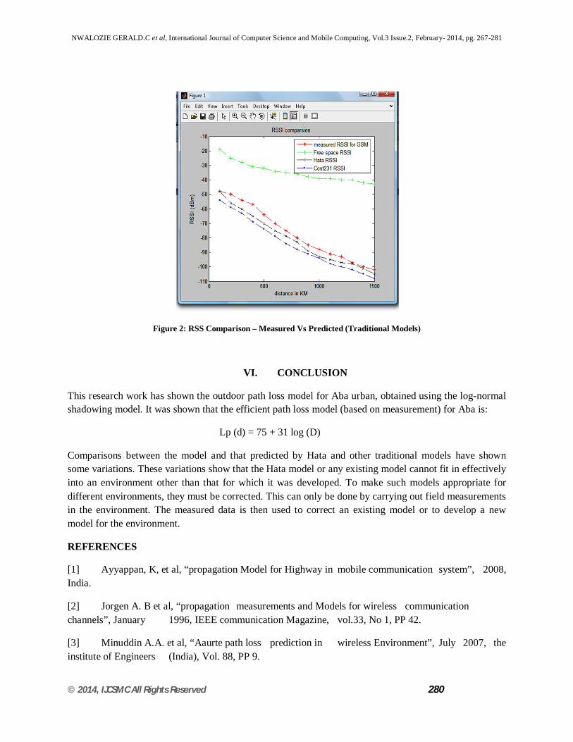
To lend credence to our derived Proposed Path Loss model, this work compared the statistically predicted result of Received Signal Strength and that of other existing (traditional) models, with the measured



results. The RSS (Pr) is therefore, calculated under the same set of transmission conditions using same simulation parameters (F=876.87MHz, hm=1.5m, hb=30m,Pt=30W) in equations 6, 11 and 20. The Pr(dBm) of the traditional models are obtained and compared with our proposed model. The Pr(dBm) values are obtained using :

Pr (dBm) = Pt (dBm) + Gt (dB) + Gr (dB) – Lp (dB)

Then, Pt (dBm) = 10 Log = 10 Log (30* 1000) = 44.77dBm ≅ 45dBm

G = 13dBd = 15dBi and G = 0dBd = 2.2dBi.

Table 3: RSSI Comparison

Distance(Km) GSM model (dBm)

Free Space

Hata Cost 231

0.10 -48 -19 -48 -54

0.20 -50 -25 -56 -59

0.30 -54 -28 -60 -63

0.40 -57 -31 -65 -69

0.50 -64 -34 -70 -74

0.60 -70 -35 -75 -74

0.70 -75 -36 -79 -79

0.80 -80 -38 -83 -84

0.90 -85 -39 -89 -88

1.00 -88 -39 -93 -91

1.10 -91 -40 -95 -94

1.20 -93 -40 -97 -98

1.30 -97 -42 -98 -100

1.40 -100 -43 -101 -102

1.50 -102 -45 -105 -108



Figure 2: RSS Comparison – Measured Vs Predicted (Traditional Models)

VI. CONCLUSION

This research work has shown the outdoor path loss model for Aba urban, obtained using the log-normal shadowing model. It was shown that the efficient path loss model (based on measurement) for Aba is:

Lp (d) = 75 + 31 log (D)

Comparisons between the model and that predicted by Hata and other traditional models have shown some variations. These variations show that the Hata model or any existing model cannot fit in effectively into an environment other than that for which it was developed. To make such models appropriate for different environments, they must be corrected. This can only be done by carrying out field measurements in the environment. The measured data is then used to correct an existing model or to develop a new model for the environment.

REFERENCES

[1] Ayyappan, K, et al, “propagation Model for Highway in mobile communication system”, 2008, India.

[2] Jorgen A. B et al, “propagation measurements and Models for wireless communication channels”, January 1996, IEEE communication Magazine, vol.33, No 1, PP 42.

[3] Minuddin A.A. et al, “Aaurte path loss prediction in wireless Environment”, July 2007, the institute of Engineers (India), Vol. 88, PP 9.



[4] A.R Mishra, “Second generation network planning and optimization (GSM)”, John Wiley and sons, February 23, 2004

[5] R.K. singh, Purnima K. sharma, “comparative Analysis of propagation path loss Models with field measured Data”, International Journal of Engineering science and Tech. Vol. 2(6), 2010, 2008-2013.

[6] M. Hata,” Empirical formula for propagation loss in land mobile radio services”, IEEE trans-veh Tech vol VT- 29, No 3, PP 317-325, any. 1980.

[7] M.G. brown, et al, “comparison of empirical propagation path loss models for fixed wireless access systems”, Vehicular Technology conference, 2005. IEEE Date: 30 may-1 June 2005 vol:1 PP 73-77

[8] Smith, M.S. et al., “A new methodology for deriving path loss models from cellular drive test data, April 2000, Proc. AP 2000, conference, Davos, Sivitzerlend.

[9] Z. Nadir, N. Elfadhil and F. Touati, “Path loss Determination, using Okumura-Hata Model and Spline Interpolation for missing data for Oman’’– Proceedings of Journal of World Congress, 2009.

[10] . V. Erceg, et al, “An Empirically based path loss model for Wireless Channels in Suburban Environment” IEEE Journal on selected areas in Communications, vol. 17, No. 7, 1999.

[11] T. L. Adebayo and F. O. Edeko, “Characterized Propagation Path Loss at 1.8GHz band for Benin”, Research Journal for Applied Sciences; 2006.

[12] D. A. Shalangwa and G. Jerome, “ Path loss Propagation model for Gombe Town, Adamawa State, Nigeria”, International Journal of Computer Science and Network Security, vol.18, No.6, 2010.

[13] Iskander M. and Yun Z., “Propagation Prediction Models for Wireless Communication Systems”, IEEE Trans on microwave theory and Techniques, Vol. 50, No. 3, march 2002

[14] Ubom E.A, Idigo V.E, Azubogu A.C.O, Ohaneme C.O and Alumona T.L “Path loss characterization of wireless propagation for South – South region of Nigeria” International Journal of Computer theory and Engineering, vol.3, No.3, June 2011.

[15] Wu, J. and Yuan, D., (1998) “Propagation Measurements and Modeling in Jinan City”, IEEE International Symposium on Personal, Indoor and Mobile Radio Communications, Boston, MA, USA, Vol. 3, pp. 1157-1159.

A Monthly Journal of Computer Science and Information ... · Cost 231 extension to Hata Model A...

Documents

Transcript of A Monthly Journal of Computer Science and Information ... · Cost 231 extension to Hata Model A...