A Monte Carlo method for solving unsteady adjoint equations 2008 - monte carlo adjoint.pdffor...
22
A Monte Carlo method for solving unsteady adjoint equations Qiqi Wang a, * , David Gleich a , Amin Saberi a , Nasrollah Etemadi b , Parviz Moin b a Institute of Computational and Mathematical Engineering, Stanford University, Stanford, CA 94305, USA b Center for Turbulence Research, Stanford University, Stanford, CA 94305, USA Received 2 June 2006; received in revised form 30 October 2007; accepted 2 March 2008 Available online 17 March 2008 Abstract Traditionally, solving the adjoint equation for unsteady problems involves solving a large, structured linear system. This paper presents a variation on this technique and uses a Monte Carlo linear solver. The Monte Carlo solver yields a forward-time algorithm for solving unsteady adjoint equations. When applied to computing the adjoint associated with Burgers’ equation, the Monte Carlo approach is faster for a large class of problems while preserving sufficient accuracy. Ó 2008 Elsevier Inc. All rights reserved. Keywords: Adjoint equation; Unsteady adjoint equation; Monte Carlo linear solver 1. Introduction Adjoint based methods are widely used tools for analyzing and controlling the behavior of many systems. In these methods, one models a system as an algebraic or differential equation, then the adjoint equation of the original problem is derived, and finally both equations are solve. From the solution of the adjoint equation, the derivative of an objective function is calculated with respect to a set of control parameters. Often this pro- cedure is called backward algorithmic (automatic) differentiation [15]. Adjoint based methods solve a large class of optimization problems, inverse problems and control problems [2,5,11,16,17,20]. Another important application of adjoint based methods is posterior error estimation. In this context, these methods are often called duality based methods [12,13,18]. They are particularly useful when the original problem is a discretized partial differential equation. When the numerical error caused by the discretization is high, we can apply automatic adaptive mesh refinement [19] based on the adjoint solution to reduce the numerical error at a fixed computational cost. Although adjoint based methods have a long history in computational sciences and engineering [3], comput- ing the solution of an adjoint equation is difficult: when the original problem is a time dependent (unsteady) 0021-9991/$ - see front matter Ó 2008 Elsevier Inc. All rights reserved. doi:10.1016/j.jcp.2008.03.006 * Corresponding author. Tel.: +1 650 796 4472. E-mail address: [email protected] (Q. Wang). Available online at www.sciencedirect.com Journal of Computational Physics 227 (2008) 6184–6205 www.elsevier.com/locate/jcp
Transcript of A Monte Carlo method for solving unsteady adjoint equations 2008 - monte carlo adjoint.pdffor...

Available online at www.sciencedirect.com
Journal of Computational Physics 227 (2008) 6184–6205
www.elsevier.com/locate/jcp
A Monte Carlo method for solving unsteadyadjoint equations
Qiqi Wang a,*, David Gleich a, Amin Saberi a, Nasrollah Etemadi b, Parviz Moin b
a Institute of Computational and Mathematical Engineering, Stanford University, Stanford, CA 94305, USAb Center for Turbulence Research, Stanford University, Stanford, CA 94305, USA
Received 2 June 2006; received in revised form 30 October 2007; accepted 2 March 2008Available online 17 March 2008
Abstract
Traditionally, solving the adjoint equation for unsteady problems involves solving a large, structured linear system.This paper presents a variation on this technique and uses a Monte Carlo linear solver. The Monte Carlo solver yieldsa forward-time algorithm for solving unsteady adjoint equations. When applied to computing the adjoint associated withBurgers’ equation, the Monte Carlo approach is faster for a large class of problems while preserving sufficient accuracy.� 2008 Elsevier Inc. All rights reserved.
Keywords: Adjoint equation; Unsteady adjoint equation; Monte Carlo linear solver
1. Introduction
Adjoint based methods are widely used tools for analyzing and controlling the behavior of many systems.In these methods, one models a system as an algebraic or differential equation, then the adjoint equation of theoriginal problem is derived, and finally both equations are solve. From the solution of the adjoint equation,the derivative of an objective function is calculated with respect to a set of control parameters. Often this pro-cedure is called backward algorithmic (automatic) differentiation [15]. Adjoint based methods solve a largeclass of optimization problems, inverse problems and control problems [2,5,11,16,17,20].
Another important application of adjoint based methods is posterior error estimation. In this context, thesemethods are often called duality based methods [12,13,18]. They are particularly useful when the originalproblem is a discretized partial differential equation. When the numerical error caused by the discretizationis high, we can apply automatic adaptive mesh refinement [19] based on the adjoint solution to reduce thenumerical error at a fixed computational cost.
Although adjoint based methods have a long history in computational sciences and engineering [3], comput-ing the solution of an adjoint equation is difficult: when the original problem is a time dependent (unsteady)
0021-9991/$ - see front matter � 2008 Elsevier Inc. All rights reserved.
doi:10.1016/j.jcp.2008.03.006
* Corresponding author. Tel.: +1 650 796 4472.E-mail address: [email protected] (Q. Wang).

Q. Wang et al. / Journal of Computational Physics 227 (2008) 6184–6205 6185
problem, solving its adjoint equation is a backward-time procedure and requires the full trajectory to be storedin memory. The trajectory is formed by the solution of the original problem at all time steps, and is often toolarge to store in memory. In [14], Griewank proposed a very interesting iterative checkpointing scheme calledrevolve for dealing with this problem. In his scheme, storing the full trajectory is avoided by iteratively solvingthe original problem. This idea made solving adjoint equations possible for larger unsteady problems. Sincethen, a number of similar schemes have been proposed [4,28]. Nevertheless, all of these schemes are significantlymore expensive than solving the original problem in terms of both memory requirements and computationaltime. As a result, if the original problem is very large in terms of the number of degrees of freedom, solvingthe adjoint equation is still prohibitively expensive.
In this paper, we propose a new method for solving the adjoint equation for unsteady problems. Instead ofcomputing an exact solution, we use a Monte Carlo method to approximate the solution. This method samplesMarkovian random walks in the space–time structure of the original problem and estimates quantities of inter-est from these samples. The method builds upon Monte Carlo linear solvers for general linear systems[10,7,27,22] and some related works [23]. We found that the Monte Carlo method is particularly suitablefor solving unsteady adjoint equations. In contrast to traditional methods used for solving the adjoint equa-tion, this method is a forward-time procedure. Amazingly, neither storing the trajectory nor iteratively solvingthe original problem is required. Therefore, the memory requirement and computational time of our MonteCarlo method are a constant multiples of the original problem (as opposed to exact solution methods wherethese requirements are log m times larger, where m is the number of time steps).
In the remainder of this paper, Section 2 introduces the unsteady adjoint equation. Section 3 describes thetraditional exact solution methods. In Section 4, we introduce our Monte Carlo method for solving adjointequations. Because many large problems arise from discretized partial differential equations, we describeour method specifically for this case. The error and variance of this method is analyzed in Section 5. In Sec-tions 6 and 7, we show the results of several numerical experiments with Burgers’ equation.
2. The unsteady adjoint equation
Consider a state vector u controlled by a control vector g via constraint or governing equation R. Theobjective function F is defined on the space of u and g. We denote this by
F ðu; gÞRðu; gÞ ¼ 0;
�ð1Þ
where F is a scalar function and R is a vector function with dimðRÞ ¼ dimðuÞ. In the context of an adjointequation, system (1) is often referred as the original problem.
Many engineering applications fit this problem type. Generally, R is an algebraic or differential equationmodeling a physical system, u is a vector describing the state of the system and g is a vector composed of aset of control parameters. In the context of computational fluid dynamics, most problems concern objectsin a flow field. In these problems, the constraint R, the Navier–Stokes equation, controls the flow field u.We are often interested in objective functions such as the lift, drag and other forces, which are possible can-didates for F . The control parameters might be the geometry of the object itself or perturbations to the bound-ary conditions.
The adjoint equation of the system (1) is defined as the linear system
oR
ou
� �T
w ¼ oF
ou
� �T
; ð2Þ
where ðoRou Þ
T is the constraint Jacobian and w is the adjoint solution.The adjoint equation is widely used in analyzing and controlling the system (1). For example, many opti-
mization problems, inverse problems and control problems require computing the derivative of the objectivefunction with respect to the control parameters of the original problem (1),
dFðuðgÞ; gÞdg
¼ oF
ogþ oF
ouduðgÞ
dg;

6186 Q. Wang et al. / Journal of Computational Physics 227 (2008) 6184–6205
where uðgÞ is an implicit function defined by R and its derivative duðgÞdg can be obtained from
0 ¼ dRðuðgÞ; gÞdg
¼ oR
ogþ oR
ouduðgÞ
dg:
Therefore, with some manipulation of the adjoint equation (2), we get
dF ðuðgÞ; gÞdg
¼ oF
og� oF
ouoR
og
� ��1oR
og¼ oF
og� wT oR
og; ð3Þ
which is a linear function of the adjoint solution. In this paper, we focus on the case when the original problem(1) is an unsteady problem; e.g. when the constraint R is a time dependent partial differential equation. In thiscase, we can order the elements of the state vector and the constraint by time steps, i.e.
u ¼ ðuð1Þ; . . . ; uðmÞÞT; R ¼ ðRð1Þ; . . . ;RðmÞÞT;
where m is the number of time steps, uðiÞ and RðiÞ are the state vector and the constraint at time step i. With thisordering, the matrix ðoRou ÞT in the unsteady adjoint equation (2) is well structured. This is because for unsteady
problems, RðiÞ only depends on the part of u up to time step i. In other words, a block of the constraint Jaco-bian J ij 6¼ 0 only if j 6 i. As a result, the Jacobian matrix oR
ou is in block-lower-triangular form.
oR
ou¼
J 11
J 21 J 22
. .. . .
. . ..
J m1. .
.J mm�1 J mm
2666664
3777775; ð4Þ
where each block describes the spatial dependence of the constraint.
J ts ¼oRðtÞ
ouðsÞ
� �:
The adjoint equation (2) now becomes
J T11 J T
21. .
.J T
m1
J T22
. .. . .
.
. .. . .
.
J Tmm
266666664
377777775
wð1Þ
wð2Þ
..
.
wðmÞ
266664
377775 ¼
bð1Þ
bð2Þ
..
.
bðmÞ
266664
377775; ð5Þ
where
bðtÞ ¼ oF
ouðtÞ
� �T
:
In this representation, the adjoint solution w is split into m parts. We call wðtÞ the adjoint solution at time stept.
Moreover, if R comes from a discretized unsteady differential equations, the Jacobian matrix is also block-banded. In this case, RðtÞ only depends on the part of u that is in a neighborhood of time step t, and J ts 6¼ 0only if s is in a neighborhood of t. Hence the Jacobian matrix has a block-bandwidth that depends on thetemporal discretization scheme. For example, if the original problem uses a one-step scheme, RðtÞ dependsonly on uðtÞ and uðt�1Þ. In this case, the block-bandwidth is two. If it is a two-step scheme, then the block-band-width is three, etc. In particular, if the differential equation is discretized using an explicit scheme, thenRðtÞ ¼ uðtÞ � f ðuðt�1Þ; . . .Þ, and the diagonal blocks of the Jacobian are identity matrices
J tt ¼oRðtÞ
ouðtÞ
� �¼ I :
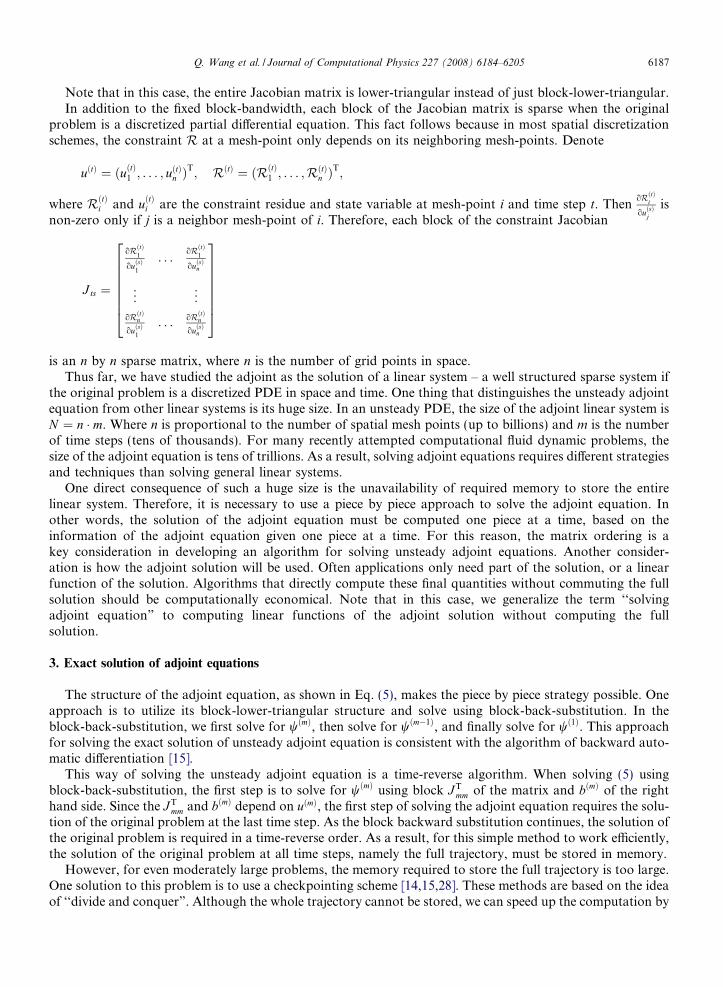
Q. Wang et al. / Journal of Computational Physics 227 (2008) 6184–6205 6187
Note that in this case, the entire Jacobian matrix is lower-triangular instead of just block-lower-triangular.In addition to the fixed block-bandwidth, each block of the Jacobian matrix is sparse when the original
problem is a discretized partial differential equation. This fact follows because in most spatial discretizationschemes, the constraint R at a mesh-point only depends on its neighboring mesh-points. Denote
uðtÞ ¼ ðuðtÞ1 ; . . . ; uðtÞn ÞT; RðtÞ ¼ ðRðtÞ1 ; . . . ;RðtÞn Þ
T;
where RðtÞi and uðtÞi are the constraint residue and state variable at mesh-point i and time step t. Then
oRðtÞi
ouðsÞj
isnon-zero only if j is a neighbor mesh-point of i. Therefore, each block of the constraint Jacobian
J ts ¼
oRðtÞ1
ouðsÞ1
. . .oRðtÞ1
ouðsÞn
..
. ...
oRðtÞn
ouðsÞ1
. . . oRðtÞn
ouðsÞn
26666664
37777775
is an n by n sparse matrix, where n is the number of grid points in space.Thus far, we have studied the adjoint as the solution of a linear system – a well structured sparse system if
the original problem is a discretized PDE in space and time. One thing that distinguishes the unsteady adjointequation from other linear systems is its huge size. In an unsteady PDE, the size of the adjoint linear system isN ¼ n � m. Where n is proportional to the number of spatial mesh points (up to billions) and m is the numberof time steps (tens of thousands). For many recently attempted computational fluid dynamic problems, thesize of the adjoint equation is tens of trillions. As a result, solving adjoint equations requires different strategiesand techniques than solving general linear systems.
One direct consequence of such a huge size is the unavailability of required memory to store the entirelinear system. Therefore, it is necessary to use a piece by piece approach to solve the adjoint equation. Inother words, the solution of the adjoint equation must be computed one piece at a time, based on theinformation of the adjoint equation given one piece at a time. For this reason, the matrix ordering is akey consideration in developing an algorithm for solving unsteady adjoint equations. Another consider-ation is how the adjoint solution will be used. Often applications only need part of the solution, or a linearfunction of the solution. Algorithms that directly compute these final quantities without commuting the fullsolution should be computationally economical. Note that in this case, we generalize the term ‘‘solvingadjoint equation” to computing linear functions of the adjoint solution without computing the fullsolution.
3. Exact solution of adjoint equations
The structure of the adjoint equation, as shown in Eq. (5), makes the piece by piece strategy possible. Oneapproach is to utilize its block-lower-triangular structure and solve using block-back-substitution. In theblock-back-substitution, we first solve for wðmÞ, then solve for wðm�1Þ, and finally solve for wð1Þ. This approachfor solving the exact solution of unsteady adjoint equation is consistent with the algorithm of backward auto-matic differentiation [15].
This way of solving the unsteady adjoint equation is a time-reverse algorithm. When solving (5) usingblock-back-substitution, the first step is to solve for wðmÞ using block J T
mm of the matrix and bðmÞ of the righthand side. Since the J T
mm and bðmÞ depend on uðmÞ, the first step of solving the adjoint equation requires the solu-tion of the original problem at the last time step. As the block backward substitution continues, the solution ofthe original problem is required in a time-reverse order. As a result, for this simple method to work efficiently,the solution of the original problem at all time steps, namely the full trajectory, must be stored in memory.
However, for even moderately large problems, the memory required to store the full trajectory is too large.One solution to this problem is to use a checkpointing scheme [14,15,28]. These methods are based on the ideaof ‘‘divide and conquer”. Although the whole trajectory cannot be stored, we can speed up the computation by

6188 Q. Wang et al. / Journal of Computational Physics 227 (2008) 6184–6205
restarting from a set of checkpoints. Additional forward iterations of the original problem move the solutionbetween checkpoints [4].
In 1992, Griewank [14] first proposed the scheme revolve which uses this idea to achieves optimal logarith-mic behavior in terms of both computational time and memory requirement. Revolve and many other check-pointing schemes proposed since then use Oðlog mÞ times the memory and computational time of the originalproblem. Using these schemes, the cost of solving the adjoint equation is only a relatively small factor timesthe cost of solving the original problem, even if the number of time steps is large.
4. Monte Carlo method for adjoint equation
In this section, we propose a Monte Carlo method for solving the unsteady adjoint equation. Both thememory requirement and computational time of this scheme are Oð1Þ times that of the original problem, inde-pendent of the number of time steps of the original problem. As demonstrated in Section 7, our Monte Carlomethod has better scaling efficiency than the optimal exact solution method.
Monte Carlo methods have already been shown to be efficient for solving many systems of linear equations,especially when the system is very large and the required precision is relatively low [27,7,1]. These methodscraft statistical estimators whose mathematical expectation is a component of the solution vector. Randomsampling of these estimators yields approximate solutions [27,24,29]. The main ideas of these methods wereproposed by von Neumann and Ulam and are extended by Forsythe and Liebler [10].
Using Monte Carlo methods has several known advantages for solving linear equations. First, the compu-tational cost of obtaining one component of the solution vector using these methods is independent of the sizeof the linear system [27]. More precisely, it is OðqlÞ, where q is the number of random walks and l is theirlength. Both q and l are independent of the size of the linear system, and can be controlled to obtain anydesired precision. Also, Monte Carlo methods are known for their parallel nature. It is often very easy to par-allelize them in a coarse grained manner. Even early in 1949, Metropolisand and Ulam [21] noticed the par-allelism inherent in this method.
In addition to these advantages, Monte Carlo methods are particularly suitable for solving the unsteadyadjoint equation for two reasons. One is that the Monte Carlo method used in this paper to solve the unsteadyadjoint equation is a forward-time procedure. In this procedure, we only use the information necessary toadvance to the next time step, which enables us to solve the adjoint equation at the same time as we solvethe original equation. Thus we do not need to store full trajectory, neither do we need to iteratively resolvethe original problem. This is one great advantage over the traditional method. Secondly, we can directly com-pute the inner product of the solution w with a given vector c, without computing w. And the cost of comput-ing cTw using this method is only OðqlÞ, which is the same as the cost of computing one component of thesolution vector. In computing dF
dg using Eq. (3) we can take advantage of this by representing wT oRog as the inner
product of w with dimðgÞ given vectors
wT oR
og¼ wT oR
og1
;wT oR
og2
; . . . ;wT oR
ogn
� �; where n ¼ dimðgÞ
When the dimension of the control vector dimðgÞ is much smaller than the dimension of the state vectordimðuÞ, we can save a lot of computational cost by directly computing wT oR
og . This is useful in applications suchas wall control for drag reduction [5,2].
In the remainder of this section, Section 4.1 introduces the (preconditioned) Neumann series representationof the solution. In Section 4.2, we construct the Markovian random walk and the D estimator. We prove thatthe D estimator is an unbiased estimator to the Neumann series representation of the solution. These discus-sions are valid for general linear systems and are presented in more detail in [22]. Section 4.3 describes ourMonte Carlo algorithm designed specifically for solving unsteady adjoint equations using the D estimator.Section 5.2 discusses the choice of transition probabilities of the Markovian random walk based on the theoryof minimum probable error [6]. Section 5.4 discusses choice of preconditioner used in Neumann series repre-sentation for our Monte Carlo method. Finally, in Section 6 we fully specify our Monte Carlo algorithm usedfor Burgers’ equation.

Q. Wang et al. / Journal of Computational Physics 227 (2008) 6184–6205 6189
4.1. Neumann series representation
To simplify notation, let
�A ¼ oR
ou
� �T
and �b ¼ oF
ou
� �T
in adjoint equation (2). The adjoint equation simplifies to
�Aw ¼ �b:
We multiply both sides by a block-diagonal preconditioner matrix P, that is easy to invert and preserves theblock-upper-triangular structure of the Jacobian �A. Denote
A ¼ I � P �A and b ¼ P�b: ð6Þ
We note that A has the same block-upper-triangular and block-banded structure of �A. Now the adjoint equa-tion becomesw ¼ Awþ b: ð7Þ
The solution w to the equation above can be expanded in a Neumann series:w ¼ bþ Abþ A2bþ A3bþ � � � : ð8Þ
The Neumann series converges and (8) is valid if and only if the spectral radius of A is less than one. Whenit converges, the Neumann series (8) is the solution of the adjoint equation (7). Note that the inner product ofw with a given vector c can be represented as
cTw ¼ cTðbþ Abþ A2bþ A3bþ � � �Þ ¼X1k¼0
cTAkb ð9Þ
The Monte Carlo method in this paper is a random sampling of this infinite series by a Markovian randomwalk.
4.2. Markovian random walk and D estimator
For a given vector c, we use Markovian random walks to create random samples of an estimator D intro-duced in (18) whose mathematical expectation are the inner product of the solution w with the given vector c,i.e. EðDÞ ¼ cTw. In particular, when c ¼ ei, EðDÞ ¼ wTei ¼ wi, and we compute a component of the solutionvector. The Markovian random walks have a finite state space with size N þ 1, where N is the size of theadjoint equation. If we label the states as 1; 2; . . . ;N þ 1, each of the first N states correspond to a componentof the adjoint equation. The special state, a final exit state, gets label N þ 1. The random walks begin from abirth probability r, and follow a transition probability p, where pði; jÞ is the transition probability from state i
to state j. r and p must satisfy the following conditions [22]:
ð1Þ 0 6 rðjÞ; pði; jÞ 6 1 for all i; j; ð10Þ
ð2ÞXNþ1
j¼1
pði; jÞ ¼ 1 for all i; ð11Þ
ð3ÞXN
i¼1
rðiÞ ¼ 1; ð12Þ
ð4Þ pðN þ 1;N þ 1Þ ¼ 1; ð13Þð5Þ pði; jÞ 6¼ 0() Aij 6¼ 0 and rðiÞ 6¼ 0() ci 6¼ 0; ð14Þ
where Aij is the i; jth entry of the matrix A, and ci is the ith component of the vector c In the four conditionsabove, the first three define r and p as birth and transition probabilities. The fourth condition defines the stateN þ 1 as the final exit state. We note that the probability that the Markovian random walk transits from state j

6190 Q. Wang et al. / Journal of Computational Physics 227 (2008) 6184–6205
to the final exit state is pðj;N þ 1Þ ¼ 1�PN
i¼1pði; jÞ. Once it reaches the final exit state, it always stays therewith probability 1. When this happens, we say that the random walk was absorbed in state j. The last condi-tion means that the random walks always stay tied to the matrix, which allows us to go from the random walkmodel described by p and a to the Neumann series (9) that involves Aij and ci.
Now we will relate the random walk to the components of the matrix A. Indeed, let the Markov chain be
a ¼ a0; a1; . . . ; an; . . .ð Þ
andi ¼ ði0; i1; . . . ; il;N þ 1;N þ 1; . . .Þ; 1 6 ij 6 N
be a typical path of the Markov chain that begins at state i0 and is absorbed at state il. The probability that theMarkov chain takes this path is
Pða ¼ iÞ ¼ rði0Þpði0i1Þpði1i2Þ � � � pðil�1IlÞpðil;N þ 1Þ:
We definewij ¼Aij
pði;jÞ if pði; jÞ 6¼ 0
0 if pði; jÞ ¼ 0
(
and as in [22], we define the weight W k as a random variables on the space of random walks a:
W kðaÞ ¼ca0
rða0ÞYk
j¼1
wajaj�1; 0 6 k 6 l ð15Þ
The following proposition gives us insight on why we define the weight in this way.
Proposition 4.1. Assume conditions (10)–(14) are satisfied. Denote ð�Þj as the jth component of a vector, and ð�Þijas the i; j entry of a matrix. Then
EðW kIfak¼jgÞ ¼ ðcTAkÞj ð16Þ
In particular, if c ¼ ei,
EðW kIfak¼jgÞ ¼ ðAkÞij ð17Þ
Proof 4.2. Since W 0 ¼ca0
rða0Þand Pða0 ¼ jÞ ¼ rðjÞ,
E½W 0Ifa0¼jg� ¼ Pða0 ¼ jÞ cj
rðjÞ ¼ cj
So (16) holds for k ¼ 0. Assume it holds for certain k, we prove it holds for k þ 1.
E½W kþ1Ifakþ1¼jg� ¼ EX
i
ðIfak¼i;akþ1¼jgW kwði; jÞÞ" #
¼X
i
E½Ifak¼i;akþ1¼jgW k�Aij
pði; jÞ
By using the tower property of conditional expectations, ‘‘taking out what is known” and applying Markovproperty, we have
E½Ifak¼i;akþ1¼jgW k� ¼ E½Ifak¼igW k�pði; jÞ:
Therefore, by the induction hypothesis,
E½W kþ1Ifakþ1¼jg� ¼X
i
E½Ifak¼igW k�Aij ¼X
i
ðcTAkÞiAij ¼ ðcTAkþ1Þj:
Thus we conclude that (16) holds true for all k P 0. (17) follows trivially. h
This tells us that W kIfak¼jg is in fact a randomly sparsified version of vector cTAk. The randomly sparsifiedvector contains only one non-zero entry. In every step of the random walk, W kIfak¼jg is multiplied by A, andfurther sparsified. We can think of it as the sparsified version of cTAk is multiplied by A, by which we get an

Q. Wang et al. / Journal of Computational Physics 227 (2008) 6184–6205 6191
approximation of cTAkþ1, and then sparsify it. Because the Neumann series (9) gives us a relationship betweencTw and cTAk, we can use this relationship to build an estimator for cTw in terms of W kIfak¼jg, which is arandomly sparsified version of cTAk.
Definition 4.3. Define the D estimator by
DðaÞ ¼X1k¼0
W kðaÞbak ð18Þ
where a ¼ ða0; a1; . . .Þ is the random walk; ðb1; . . . ; bNÞT is the right hand side of equation (7) and bNþ1 ¼ 0.
Now we prove the main theorem that supports the Monte Carlo method.
Theorem 4.4. Assume that the Neumann series (8) converges for jAj, and conditions (10)–(14) are satisfied. Then
the expectation of the D estimator
EðDðaÞÞ ¼ cTw
where w is the solution of Eq. (7).
Proof 4.5. Since bak ¼P
jIfak¼jg, the expectation of the D estimator can be represented as
E½D� ¼ EX1k¼0
W kbak
" #¼ E
X1k¼0
Xj
W kIfak¼jgbj
" #¼X1k¼0
Xj
E W kIfak¼jg� �
bj:
The condition that the Neumann series converges for jAj justifies the exchange of infinite sum and expectationby dominated convergence theorem. It follows from Proposition 4.1 that
E½D� ¼X1k¼0
Xj
ðcTAkÞjbj ¼X1k¼0
cTAkb;
which is the Neumann series expansion (9). Thus we have
E½D� ¼ cTw; ð19Þ
i.e. D is an unbiased estimator of cTw. hThis theorem suggests that we can use Monte Carlo method based on the D estimator to approximate cTw
cTw � 1
q
Xq
p¼1
Dða½p�Þ;
where a½p�; 1 6 p 6 q are independent identically distributed random walks. And the following corollary is adirect consequence of Theorem 4.4 and the strong law of large number.
Corollary 4.6. Under the conditions of Theorem 4.4, the estimated solution by the Monte Carlo method
1
q
Xq
p¼1
Dða½p�Þ ! cT/
almost surely as q!1.
This result justifies our Monte Carlo approach for solving adjoint equation by saying that as the number ofrandom walks increases, the solution of the Monte Carlo method asymptotically converges to the exactsolution.
4.3. Monte Carlo algorithm
In this section, we explain the Monte Carlo algorithm for solving the unsteady adjoint equation based onthe D estimator constructed in the last section.

6192 Q. Wang et al. / Journal of Computational Physics 227 (2008) 6184–6205
We note that condition (14) of the transition probability matrix guarantees that P has the same block-upper-triangular and block-banded structure as matrix A. We remember that the components of u are orderedby time steps. As a result, random walks defined by this transition probability matrix can only possibly walk tolater time steps (upper-diagonal blocks of P are non-zeros), or walk within the same time step (diagonal blocksof P are non-zero), but never walk backwards to previous time steps (lower-diagonal blocks of P are alwayszero). Therefore, the Markovian random walks only go forward in time. This makes the following forward-time Monte Carlo algorithm possible.
In this algorithm, we generate q independent identically distributed random walks a½p�; 1 6 p 6 q. Each ofthem has transition probabilities pði; jÞ and birth probabilities rðiÞ that satisfies the conditions (10)–(14). Wewill discuss the choices for r and p in the next section. We denote ak½p� as the current position of random walka½p�, and we say that a random walk a½p� is at time step t if ak½p� is in the range of indices that represent timestep t. Let W ½p� denote W kða½p�Þ, the weight of random walk at current step. D½p� stores the accumulative sumof the D estimator (18), which equals to DðaÞ after the random walk is absorbed.
(1) For each 1 6 p 6 q, choose a0½p� randomly by birth probability vector r, and initialize
W ½p� ¼ ca0½p�=rða0½p�Þ; D½p� ¼ W ½p�ba0½p�:
Then start from t ¼ 1, do step 2–4, until done with the last time step t ¼ m.(2) Solve the original problem at time step t, which enables us to compute the corresponding blocks
of matrix A and p.(3) For each random walk a½p� that is at time step t, choose its next state akþ1½p� randomly by
transition probabilities p. If akþ1½p� is not the final exit state, update
W ½p� ¼ W ½p�wak ½p�akþ1½p�; D½p� ¼ D½p� þ W ½p�bakþ1½p�:
If akþ1½p�0 is the final exit state, the random walk is absorbed and we freeze D½p�.(4) Repeat step 3 until all random walks at time step t are either absorbed or left the time step. If t < m,
then let t ¼ t þ 1 and go to step 2.(5) After done with the last time step m, all random walks are absorbed. Compute the sample mean
of the estimators 1q
Pqp¼1D½p�, which is our approximation to cTw.
It is clear that this is a forward-time algorithm in which we only need to store the current time steps of theoriginal problem and no iterations are needed. Further, it directly yields the inner product of the solution withthe given vector. Indeed, there is no difficulty with this algorithm to solve multiple linear functions of the solu-tion vector at the same time. This property is useful in many adjoint based methods. For example, in comput-
ing dFðuðgÞ;gÞdg using formula (3), we can use the Monte Carlo method to directly compute wT oR
og , which is the
inner product of the adjoint solution w with oRogi; i ¼ 1; . . . ; dimðgÞ. This can be directly obtained from the
algorithm described above. The cost of this algorithm is OðnqlÞ plus the cost of the original problem, wheren is the dimension of the control vector; q is the number of random walks for each evaluation of inner productand l is the average length of the random walk, which is proportional to the number of time steps m of theoriginal problem. When the dimension of the control vector is much smaller than the mesh size, and therequired precision is relatively low (which allows us to choose a small q), the cost of solving the adjoint equa-tion in this algorithm is a small overhead. This is particularly attractive especially compared to solving theexact solution of the unsteady adjoint equation, which is significantly more costly in computation time andstorage than the original problem.
5. Analysis of the Monte Carlo method
In the last section, we derived the algorithm of using random walk Monte Carlo to solve the discrete adjointequation, and theoretically proved that as the number of samples increases, the solution obtained by our methodconverges asymptotically to the exact solution. In practice, however, it is only possible to run a finite number ofrandom walks with limited computational resources. In this section, we address the following questions: how

Q. Wang et al. / Journal of Computational Physics 227 (2008) 6184–6205 6193
much error is made by running a finite number of random walks, and how this error can be controlled andminimized.
Before we start, we definition the probable error in order to quantify the difference between the MonteCarlo approximation and the exact solution of the adjoint equation.
Definition 5.1. Let I be the value to be estimated by Monte Carlo method, and D be its unbiased estimator.The probable error for the Monte Carlo method is defined to be
r ¼ sup s : PðjI � DjP sÞ > 1
2
� �ð20Þ
The probable error specifies the range which contains 50% of the possible values of the estimator. In thecase of continuous distribution, this is equivalent to the definition in [9,25].
The probable error is closely related to the variance of the estimator. Suppose D1; . . . ;Dq are independentand identically distributed samples of D, If the variance of estimator D is bounded, the Central Limit Theorem
P
PDi
q� I 6 x
� �! UðxÞ
holds. When q is large, the probable error of the average of the q samples is [9,27]
r � 0:6745VarD
q
� �1=2
: ð21Þ
Therefore, the probable error decreases when the number of samples q increases or when the variance of theestimator D decreases. Using this formula, we can estimate and control the probable error of our Monte Carlomethod by estimating the variance of the D estimator.
In the rest of this section, we focus on the variance of the D estimator. To make mathematical derivationcleaner, we denote
pij ¼ pði; jÞ
to be the transition probability from state i to state j,pi ¼ pði;N þ 1Þ
to be the transition probability from state i to the final exit state, andri ¼ rðiÞ
to be the birth probability at state i.5.1. Variance decomposition
Suppose the mean and variance of the D estimator of a random walk starting from state i are EiðDÞ andViðDÞ, respectively. Since the Markov chain at state i has pi probability of going to the final exit state andpij probability of going to the jth state, we know
EiðDÞ ¼ pi
1
pi
bi
� �þX
j:Aij 6¼0
pij
Aij
pij
EjðDÞ !
¼ bi þX
j:Aij 6¼0
AijEjðDÞ;
which corresponds to the linear equation (7) we want to solve. Apply the same analysis to the expectation ofD2, we can obtain a formula for the variance of the D estimator,
ViðDÞ ¼ Ei D2�
� EiðDÞ2 ¼ pibi
pi
� �2
þX
j:Aij 6¼0
pij
A2ij
p2ij
EjðD2Þ !
� EiðDÞ2
¼ b2i
pi
þX
j:Aij 6¼0
A2ij
pij
EjðDÞ2 � EiðDÞ2 !
þX
j:Aij 6¼0
A2ij
pij
VjðDÞ !
: ð22Þ

6194 Q. Wang et al. / Journal of Computational Physics 227 (2008) 6184–6205
We can see that the variance of a random walk starting at state i comes from two parts, The first part
Vð1Þi ðDÞ ¼
b2i
pi
þX
j:Aij 6¼0
A2ij
pij
EjðDÞ2 � EiðDÞ2: ð23Þ
This part of variance is caused by the first step of the random walk. The second part
Vð2Þi ðDÞ ¼
Xj:Aij 6¼0
A2ij
pij
VjðDÞ ð24Þ
is a weighted average of the variance of random walks starting from all the states that state i leads to. This partof variance is caused solely by the random walk starting from the second step.
Similarly, we can calculate the variance of the D estimator of a random walk starting with birth probabilityri,
VrðDÞ ¼ Er D2�
� ErðDÞ2 ¼Xi:ri 6¼0
ric2
i
r2i
Ei D2� � �
� ErðDÞ2
¼Xi:ri 6¼0
c2i
riEiðDÞ2 � ErðDÞ2
!þ
Xi:ri 6¼0
c2i
riViðD2Þ
!; ð25Þ
where EiðDÞ and ViðDÞ are the mean and variance of the random walk starting deterministically from the statei. We can see that the variance of a random walk starting with birth probability ri also comes from two parts.The first part
Vð1Þr ðDÞ ¼Xi:ri 6¼0
c2i
riEiðDÞ2 � ErðDÞ2 ð26Þ
is caused by the randomness of the birth state. The second part
Vð2Þr ðDÞ ¼Xi:ri 6¼0
c2i
riViðD2Þ ð27Þ
is a weighted average of the variance of random walks starting from all the possible birth states. This part ofvariance is caused by the random walk starting from the each possible birth states.
Based on this split of variance, the next section discusses choice of transition and birth probabilities pi andri that reduces each component of the decomposition.
5.2. Choice of transition and birth probabilities
Finding the probabilities that make the variance as small as theoretically possible has been shown to beimpractically time consuming for Monte Carlo linear solvers [6,8]. For this reason, we focus on finding ‘almostoptimal’ transition and birth probabilities by minimizing upper bounds of the variances.
The upper bounds on which we base our almost optimal transition probabilities are
Vð1Þi ðDÞ ¼
b2i
pi
þX
j:Aij 6¼0
A2ij
pij
EjðDÞ2 !
� EiðDÞ2 6b2
i
pi
þX
j:Aij 6¼0
A2ij
pij
!B2 � EiðDÞ2
and
Vð2Þi ðDÞ ¼
Xj:Aij 6¼0
A2ij
pij
VjðDÞ 6X
j:Aij 6¼0
A2ij
pij
!maxj:Aij 6¼0
VjðDÞ;
where
B ¼ max jEjðDÞj

Q. Wang et al. / Journal of Computational Physics 227 (2008) 6184–6205 6195
These bounds are chosen because individual EjðDÞ2 and VjðDÞ are not known a priori. They are thereforesubstituted by a common upper bound. The optimal pij and pi for these upper bounds, under the constraints
1 (28
Xj
pij þ pi ¼ 1 and pij P 0;
are given by the formulae1
p�ij ¼jAijjB
jbij þP
jjAijjBð28Þ
and
p�i ¼jbij
jbij þP
jjAijjB: ð29Þ
These are the almost optimal transition probabilities. Note that since B is not known a priori, it needs to beestimated unless bi ¼ 0.
Similarly, we construct upper bounds for Vð1Þr ðDÞ and Vð2Þr ðDÞ:
Vð1Þr ðDÞ ¼Xi:ri 6¼0
c2i
riEiðDÞ2
!� ErðDÞ2 6
Xi:ri 6¼0
c2i
ri
!B2 � ErðDÞ2
Vð2Þr ðDÞ ¼Xi:ri 6¼0
c2i
riViðD2Þ 6
Xi:ri 6¼0
c2i
ri
!max ViðD2Þ�
The almost optimal birth probabilities that minimizes these upper bounds are given by the formula
r�i ¼jcijP
ijcijð30Þ
Because the almost optimal transition and birth probabilities minimize upper bounds of the estimator vari-ance, we use this choice of probabilities in all our numerical experiments presented later in this paper.
5.3. Growth of variance
This section studies how the variance of our D estimator can grow assuming the almost optimal transitionand birth probabilities derived in the last section. First, we plug the optimal probabilities into the upperbounds of V
ð1Þi and V
ð2Þi , we get
Vð1Þi ðDÞ 6 jbij þ CiBð Þ2 � EiðDÞ2
and
Vð2Þi ðDÞ 6
jbijBþ Ci
� �Ci max
j:Aij 6¼0VjðDÞ;
where
Ci ¼X
j
jAijj:
The total variance is the sum of the two components of the variance decomposition, thus
ViðDÞ 6 ðjbij þ CiBÞ2 � EiðDÞ2 �
þ jbijB
Ci þ C2i
� �maxj:Aij 6¼0
VjðDÞ: ð31Þ
) and (29) together minimizes upper bound of Vð1Þi ðDÞ; (28) alone minimizes upper bound of V
ð2Þi ðDÞ under the constraints.

6196 Q. Wang et al. / Journal of Computational Physics 227 (2008) 6184–6205
This equation characterize the growth of variance as the Monte Carlo random walk proceeds. In the case ofexplicit time stepping, all j such that Aij 6¼ 0 are in the next time step of i. As the random walk proceed through
time steps, the variance can suffer from exponential growth if the multiplicative factor ðjbijB
Ci þ C2i Þ is greater
than 1. If this is the case, the probable error can be too large for our Monte Carlo method to be practical. Onthe other hand, if this factor is less or equal to 1, the variance grow at most linearly. For this reason, the size ofmultiplicative factor is critical in the efficiency of our Monte Carlo method.
In the case of conservation law PDEs discretized with a positive coefficient scheme, we know the size of thismultiplicative factor. The discrete conservation property guarantees that
2 No
Xj
Aij ¼ 1;
for all but boundary grid points. Also, all Aij are non-negative in a positive coefficient scheme. As a result ofthese two properties,
Ci ¼X
j
jAijj ¼X
j
Aij ¼ 1: ð32Þ
In addition, if the adjoint equation does not have a source term, then bi ¼ 0, and the multiplicative factor
jbijB
Ci þ C2i ¼ 1:
This implies that the probable error of our Monte Carlo method does not increase exponentially in this case.This is indeed true, as seen in our numerical experiments, that the error of our Monte Carlo adjoint solverdecreases as the number of time steps gets larger. In case the adjoint equation have a source term, the discret-ized source term bi is of order of Dt, thus the multiplicative factor
jbijB
Ci þ C2i ¼ 1þOðDtÞ:
This suggests that for a fixed T, as the discretization refines, the total amount of variance growth remainbounded.
For systems other than scalar transport equations, Eq. (32) may not be true. In many cases, a proper choiceof preconditioner is required to prevent exponential growth of variance.
5.4. Choice of preconditioner
The choice of the preconditioner matrix P2 in Eq. (6) controls the behaviors of the Neumann series, andinfluences the variance growth of the estimator D. A good choice can improve the precision of the resultand reduce the cost by requiring fewer samples, while a bad choice can make the variance grow exponentially.Thus, the main purposes of the preconditioner is to control the multiplicative factor in the variance growth byreducing Ci. Just like choosing a preconditioner a linear system, there is no universal best choice. Still, thereare a few preconditioners that we wish to mention in the setting of unsteady adjoint equation.
First of all, if the Jacobian matrix is diagonal dominant, a possible choice of preconditioner is the inverse ofthe diagonal part of the Jacobian. This method is called diagonal splitting. Diagonal splitting makes the Neu-mann series equivalent to the Jacobian iteration scheme, which has guaranteed convergence for diagonal dom-inant matrices.
Tan proposes a relaxed Monte Carlo linear solver in [9,27], which is equivalent to choosing a diagonal pre-conditioner that is not equal to the diagonal part of the Jacobian matrix. It was shown that this approach hasimproved performance over diagonal splitting for many problems.
Srinivasan [26] studied non-diagonal splitting Monte Carlo solvers, which is equivalent to choosing the pre-conditioner to be inverse of the diagonal and first sub-diagonal or super-diagonal of �A. His approach is suit-
t to be confused with the transition probability matrix P.
Q. Wang et al. / Journal of Computational Physics 227 (2008) 6184–6205 6197
able for a larger class of problems than diagonal conditioning. We have not yet investigated the last two moreadvanced preconditioner in the context of solving unsteady adjoint equations.
In the context of partial differential equations, choosing a preconditioner that transforms the random walkinto the frequency space is an ideal currently being investigated. Preliminary results show that this precondi-tioner may be a solution to certain problems on which achieving a bounded variance growth using existingpreconditioners is difficult.
6. Example of Monte Carlo algorithm: Burgers’ equation
In this section, we demonstrate a concrete example of the Monte Carlo algorithm for solving adjoint equa-tions. The example is Burgers’ equation
Rðx; tÞ ¼ ut þu2
2
� �x
¼ 0;
discretized temporally by the forward Euler scheme, and spatially by the first order up-winding scheme. Ouroriginal problem is the fully discretized equation
RðtÞi ¼ uðtÞi � uðt�1Þ
i þ DtDx
f ðt�1Þiþ1
2
� f ðt�1Þi�1
2
�¼ 0; t ¼ 1; 2; . . . ;m; ð33Þ
where f is the numerical flux computed using the up-winding formula
f ðtÞiþ1
2
¼12ðuðtÞi Þ
2 if uðtÞi þ uðtÞiþ1 > 0
12ðuðtÞiþ1Þ
2 if uðtÞi þ uðtÞiþ1 6 0:
(
In this case, the full state vector u is
u ¼ ðuð1Þ1 ; . . . ; uð1Þn ; uð2Þ1 ; . . . ; uð2Þn ; . . . ; uðmÞ1 ; . . . ; uðmÞn ÞT
and the full constraint is
R ¼ ðRð1Þ1 ; . . . ;Rð1Þn ; Rð2Þ1 ; . . . ;Rð2Þn ; . . . ; R
ðmÞ1 ; . . . ;RðmÞn Þ
T
where n is the number of mesh points, and m is the number of time steps. The size of the adjoint equation as alinear system is N ¼ mn.
For this example, we will analyze the structure of the adjoint equation, derive the birth probability matrixand transition probability matrix, and walk through the Monte Carlo algorithm. Let us begin with the con-straint Jacobian matrix. The forward Euler temporal discretization scheme is a one-step scheme, and the con-straint (33) at a time step t only depends on u at time step t and t � 1. Hence, the only non-zero blocks in the
Jacobian (4) are J tt and J tt�1; t ¼ 1; . . . ;m. Moreover, the equation is discretized using explicit scheme, sooRðtÞi
ouðtÞj
is non-zero only if i ¼ j. Therefore, the diagonal blocks of the Jacobian are identity matrices,
J tt ¼oRðtÞ
ouðtÞ¼ I :
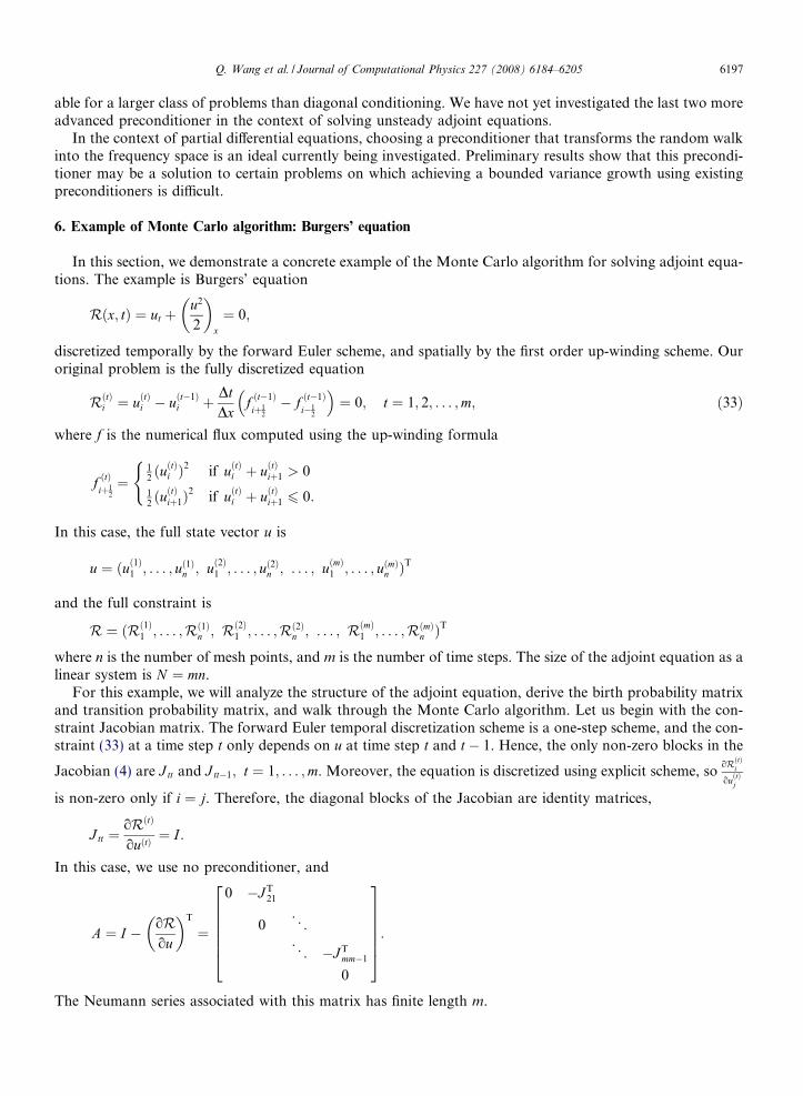
In this case, we use no preconditioner, and
A ¼ I � oR
ou
� �T
¼
0 �J T21
0 . ..
. ..
�J Tmm�1
0
2666664
3777775:
The Neumann series associated with this matrix has finite length m.

6198 Q. Wang et al. / Journal of Computational Physics 227 (2008) 6184–6205
Each block J Ttt�1 in this matrix is well structured. We note that the residue (33) at mesh-point i only depends
on u at mesh-point i� 1; x and iþ 1. ThusoRðtÞi
ouðtÞj
is non-zero only if i� 1 6 j 6 iþ 1, and the off diagonal blocks
J tt�1 are tri-diagonal matrices with entries
oRðtÞi
ouðt�1Þi�1
¼ �aðtÞiDtDx
uðtÞi�1;
oRðtÞi
ouðt�1Þi
¼ �1� bðtÞiDtDx
uðtÞi ;
oRðtÞi
ouðt�1Þiþ1
¼ �cðtÞiDtDx
uðtÞi�1;
ð34Þ
where
aðtÞi ¼�1 if uðtÞi�1 þ uðtÞi > 0
0 if uðtÞi�1 þ uðtÞi 6 0
(
bðtÞi ¼1 if uðtÞi�1 þ uðtÞi > 0 and uðtÞi þ uðtÞiþ1 > 0
�1 if uðtÞi�1 þ uðtÞi 6 0 and uðtÞi þ uðtÞiþ1 6 0
0 otherwise
8>><>>:
cðtÞi ¼1 if uðtÞi þ uðtÞiþ1 6 0
0 if uðtÞi þ uðtÞiþ1 > 0:
(
We compute the transition probabilities using (28), choosing the absorption probability to be 0 at t < m, and 1at t ¼ m. We get the transition probability matrix
P ¼
0 P 1 0
0 . ..
0
. ..
P m�1 0
0 1
0 0 0 0 1
266666664
377777775;
where the last row and column correspond to the final exit state, and each P t is an n by n tri-diagonal matrix.We note that following this transition probability matrix, each step of a random walk goes one time step for-ward. At the next step, a random walk either stays at the same mesh-point, or goes to its left or right neighbor,with probabilities specified by P t at the current time step. Therefore, in our Monte Carlo method, the spatialdistribution of the random walks follows transition probabilities P t at each time step, and all random walksare absorbed at the mth time step. This is consistent to the finite length of a Neumann series associated withthe matrix A.
Assume that we are interested in solving for the adjoint solution at the first time step wð1Þ, we can approx-imate it by starting q random walks from each of the n mesh-points at the first time step. Denote a½p; i� as thepth random walk starting at mesh-point i, and at½p; i� its position at time step t. The Monte Carlo algorithm inthis case is
(1) For each 1 6 p 6 q; 1 6 i 6 n, choose a0½p; i� ¼ x and initialize
W ½p; i� ¼ 1; D½p; i� ¼ bi:
Then start from t ¼ 1, do steps 2–4, until done with the last time step t ¼ m.(2) Solve the original problem at time step t for uðtÞ. Compute tri-diagonal matrix �J T
tþ1t using (34), andtransition probabilities P t at this time step using (28).

Q. Wang et al. / Journal of Computational Physics 227 (2008) 6184–6205 6199
(3) For each random walk, choose its next state atþ1½p� according to P t. Update
W ½p; i� ¼ W ½p; i�wat ½p;i�atþ1½p;i�; D½p; i� ¼ D½p; i� þ W ½p; i�batþ1½p;i�:
(4) Let t ¼ t þ 1, if t < m, go to step 2.(5) At last time step m, all random walks are absorbed. Compute the sample mean of the estima-
tors 1q
Pqp¼1D½p; i� for each i, which is our approximation to wð1Þi .
7. Numerical experiments
In this section, we use three numerical experiments to demonstrate the convergence property and scalingefficiency of our Monte Carlo adjoint solver as well as its performance in solving an inverse problem. Theseexperiments are done with Burgers’ equation, discretized with numerical scheme (33). Because we used anexplicit temporal discretization scheme for the original problem, we use no preconditioning in the Monte Car-lo algorithm (see Section 5.4). The transition probabilities and birth probabilities are chosen based on (28) and(30). The absorption probabilities are chosen to be 1 at the last time step, and 0 at other time steps except atboundaries. All experiments are done on a desktop with two Intel(R) Xeon(TM) 3.00 GHz CPUs, 2 GB mem-ory, GNU/Linux 2.6.9-42.0.10.ELsmp.
7.1. Convergence of Monte Carlo adjoint solver
This experiment demonstrates that the Monte Carlo adjoint solution converges to the exact solution as thenumber of random walk increases. We solve the Burgers’ equation with initial condition
uðx; 0Þ ¼ sinðpxÞ; x 2 ½0; 1� ð35Þ
in time interval ½0; 0:25�. First-order up-winding finite volume scheme is used on 100 grid points uniformlyspace on ½0; 1�; the CFL number for time integration is set to 0.5. On the other hand, the adjoint equationis solved with final condition/ðx; 0:25Þ ¼ exp �ðx� lÞ2
2r2
!; x 2 ½0; 1� ð36Þ
in the same time interval ½0; 0:25�, where l ¼ 0:5 and r ¼ 0:2. Both Burgers’ equation and the adjoint equationuse zero Dirichlet boundary condition.
Our Monte Carlo adjoint solver is used in four different settings. In each setting, the number of randomwalks starting from each grid point is, respectively, 1, 10, 100 and 1000. Griewank’s checkpointing adjointsolver is used to compute the exact adjoint solution. Fig. 1 plots the Monte Carlo adjoint equation in eachof the four cases on top of the exact solution. The Monte Carlo adjoint solution clearly converges towardsthe exact solution as the number of random walks increases.
The rate of this convergence is depicted in Fig. 2. The slope of the line in the log–log plot is roughly 0.5,indicating that our Monte Carlo adjoint solver converges at a rate of
ffiffiffiqp
, which is the common rate of con-vergence in Monte Carlo methods.
7.2. Scaling efficiency
By avoiding trajectory storage and re-iteration, our Monte Carlo adjoint solver is especially competitive toexact solution methods when the number of time steps is large. This efficiency is demonstrated by thisexperiment.
In this experiment, the Burgers’ equation is solved in time interval ½0; 0:25� with uniform grids of 10 differentsizes, ranging from 10 to 10,000. The CFL number for time integration is set to 0.5, thus the number of timesteps increases proportionally to the grid size. Similar to the first experiment, the initial condition for Burgers’equation is (35); the numerical scheme used is first-order up-winding finite volume. Again, we solve the adjointequation in time interval ½0; 0:25� using both our Monte Carlo solver and Griewank’s optimal checkpointing

Fig. 2. Convergence of Monte Carlo adjoint solution. The horizontal axis is q, the number of random walks starting from each gridpoints; the vertical axis is the L2 distance between Monte Carlo adjoint solution and the exact solution.
Fig. 1. Solutions of adjoint equation at time 0. Solid lines are solutions estimated by Monte Carlo method; dash lines are the exactsolution. The number of random walks starting from each grid point is top-left plot: 1; top-right plot: 10; bottom-left plot: 100; bottom-right plot: 1000.
6200 Q. Wang et al. / Journal of Computational Physics 227 (2008) 6184–6205
scheme. Two different settings, with q ¼ 1 and q ¼ 10, respectively, are used in the Monte Carlo solver. Wethen compare the time it takes using our Monte Carlo method in both settings to the time it takes usingthe optimal checkpointing scheme.
From the log–log plot in Fig. 3, we observe that the computation time of our Monte Carlo method in bothsettings is proportional to the square of grid size. This is because with fixed CFL number, the number of timesteps grow linearly to the grid size, and the computational time is proportional to the product of the grid sizeand the number of time steps. In contrast, the computation time of the optimal checkpointing scheme growsfaster, with a theoretical rate of n2 log n, where n is the grid size.

Fig. 3. The computation time of the adjoint solution as grid size increases. The dash line is the amount of time it takes to compute theexact adjoint solution using Griewank’s optimal checkpointing scheme; the solid line above it is the amount time it takes to estimate theadjoint solution using Monte Carlo method using q ¼ 10 random walks per grid point; the solid line below is the amount of time it takes toestimate the adjoint solution using Monte Carlo method using q ¼ 1 random walks per grid point. The calculation is done on a desktopwith two Intel(R) Xeon(TM) 3.00 GHz CPUs, 2GB memory, GNU/Linux 2.6.9-42.0.10.ELsmp. All calculations are single threaded.
Q. Wang et al. / Journal of Computational Physics 227 (2008) 6184–6205 6201
This scaling efficiency of our Monte Carlo method is obtained without sacrificing the accuracy of its esti-mated solution. Fig. 4 shows the L2 distance between the Monte Carlo adjoint solution and the exact solutionfor different grid sizes. As the grid size and number of time steps increases, the quality of the Monte Carloadjoint solution increases for a fixed number of random walks per grid point. This result indicates that whenthe computation upscales as the spatial and temporal resolution increases, our Monte Carlo is more compu-tationally efficient and produces more accurate estimated adjoint solution.
7.3. A Monte Carlo adjoint driven inverse problem
In this experiment, we test the performance of our Monte Carlo adjoint solver in solving a simple inverseproblem: finding the initial condition of a Burgers’ equation so that the solution at time T ¼ 0:25 matches aprescribed target function
Fig. 4. L2 estimation error of the Monte Carlo adjoint solver. The top line is the error for q ¼ 1 random walks per grid point; the bottomline is the error for q ¼ 10 random walks per grid point.

Fig. 5.iteratiotarget
6202 Q. Wang et al. / Journal of Computational Physics 227 (2008) 6184–6205
ftðxÞ ¼ exp �ðx� lÞ2
r2
!; x 2 ½0; 1�;
where l ¼ 0:5 and r ¼ 0:2. The boundary condition is zero Dirichlet at both x ¼ 0 and x ¼ 1.We solve the Burgers’ equation using first-order up-winding finite volume scheme on 100 uniformly spaced
grid points; the CFL number is set to 0.5. The adjoint solution is obtained by our Monte Carlo adjoint solver;the number of random walk starting from each grid point q is set to 1. This adjoint solution is used to drive agradient based optimization procedure to minimizes the square L2 difference between the solution at T and theprescribed function ft. In this experiment, we use the BFGS quasi-Newton algorithm provided by Pythonmodule scipy.optimize. The initial guess fed into the optimization routine is ft.
Due to insufficient precision of the gradient, calculated from the Monte Carlo adjoint solution, the optimi-zation procedure terminated after 28 iterations without reaching its default error tolerance. The result of thisoptimization procedure and the corresponding solution at T is plotted in Fig. 5. For the purpose of compar-ison, a fully converged solution at iteration 68 driven by the exact adjoint solution is plotted in Fig. 6. Despitethe wiggling fluctuations on the solution using Monte Carlo adjoint solver, it captures the shape of the solu-tion. The corresponding Burgers’ solution at T is also close to the target function. Moreover, the objectivefunction, the square L2 distance to the target function is 2:4� 10�4, more than 2 orders of magnitude smallerthan that of the initial guess, which is 7:5� 10�2. This result indicates that the Monte Carlo adjoint solution,being an approximation itself, is useful in obtaining an approximate solution of optimization and inverseproblems. The accuracy of the adjoint solution limits the accuracy of the computed gradient, preventing fullconvergence of gradient based optimization procedures.
Better convergence can be obtained if a smoothed version of the Monte Carlo adjoint solution is used tocalculate the gradient. Fig. 7 shows the solution of the same inverse problem driven by Monte Carlo adjointsolutions smoothed by a Gaussian filter. The number of random walks starting from each grid point q is stillset to 1. The r of the Gaussian filter is 0.03. This time the optimization routine terminates after 58 iterations.Although the default error tolerance is still not reached, the quality of the solution is significantly improved.The final objective function, 3:2� 10�5, is also an order of magnitude smaller than the final objective functionof the non-smoothed case.
This experiment concludes that despite being less accurate than the exact solution, the Monte Carlo adjointis capable of reducing the objective function in optimization and inverse problems. In some practical problemswhere the Monte Carlo adjoint solver is more computationally efficient, it may be desirable to use the Monte
Solving an inverse problem using Monte Carlo adjoint solver. The solid line is the solution to the inverse problem after 28 BFGSns. The dash line is the solution at time T of the Burgers’ equation with the solid line as its initial condition. The dot line is the
function ft. The dash line and dot line being close means that the solid line is an approximate solution to the inverse problem.

Fig. 7. Solving an inverse problem using smoothed Monte Carlo adjoint solver. The solid line is the solution to the inverse problem after57 BFGS iterations. The dash line is the solution at time T of the Burgers’ equation with the solid line as its initial condition. The dot line isthe target function ft. The dash line and dot line being almost on top of each other means that the solid line is an accurate approximatesolution to the inverse problem.
Fig. 6. Solving the same inverse problem using exact adjoint solution. The solid line is the solution to the inverse problem after 68 BFGSiterations (fully converged.) The dash line is the solution at time T of the Burgers’ equation with the solid line as its initial condition. Thedot line is the target function ft. The dash line and dot line lying on top of each other means that the solid line is an accurate solution of theinverse problem.
Q. Wang et al. / Journal of Computational Physics 227 (2008) 6184–6205 6203
Carlo adjoint solution to drive the optimization until further improvement is limited by its accuracy, thenswitch to an exact adjoint solver to ensure full convergence.
8. Future work
The Oð ffiffiffinp Þ convergence rate of the Monte Carlo method (21) makes it unattractive when the variance ofthe estimator D is high. This is the case when we apply our method to vector transport equations such asNavier–Stokes equations. Therefore, our future work focuses on reducing the variance of our estimator.

6204 Q. Wang et al. / Journal of Computational Physics 227 (2008) 6184–6205
(1) The variance of our estimator may be reduced by trying more advanced preconditioners [27,26], whichcan improve the convergence of the Neumann series. We are particular interested in investigating pre-conditioners in the case of vector partial differential equations, such as Navier–Stokes equation.
(2) We are interested in investigating Monte Carlo methods that are not based on the Neumann series.These methods are especially useful in case the Neumann series have poor convergence.
Our ultimate goal is to use this method in large simulations of physical systems, such as aerodynamic sim-ulations, turbulence simulations and fluid-structure coupled simulations.
9. Conclusion
The Monte Carlo method is an efficient method to approximate the solution of the adjoint equation. Thebiggest advantages of this method are
(1) By only advancing forward in time, it avoids storing the full trajectory or iterating the original problem.(2) It is easy to compute only part of the adjoint solution, or a linear function of the solution. This saves
computation time in practice.(3) It is conceptually easy to parallelize.
As we have demonstrated through our numerical experiments, our Monte Carlo method has better scalingefficiency than exact solution methods. By sacrificing some accuracy, choosing Monte Carlo adjoint solver inlarge scale calculations can be rewarding in terms of computation time and memory usage. This has been dem-onstrated in Burgers’ equation. If this method can be efficiently generalized to vector transport equations, itwill make very large scale calculation of their adjoint equations feasible.
Acknowledgment
This work is supported by US Department of Energy’s ASC Program at Stanford.
References
[1] V.N. Alexandrov, Efficient parallel Monte Carlo methods for matrix computations, Mathematics and Computers in Simulation 47(1998) 113–122.
[2] T. Bewley, P. Moin, R. Temam. Dns-based predictive control of turbulence: and optimal benchmark for feedback algorithms, AnnualResearch Briefs, Center of Turbulence Research, Stanford, 1993, pp. 3–14.
[3] A.E. Bryson, M.N. Desai, W.C. Hoffman, Energy state approximation in performance optimization of supersonic aircraft, Journal ofAircraft 6 (12) (1969) 488–490.
[4] I. Charpentier, Checkpointing schemes for adjoint codes: application to the meteorological model meso-nh, SIAM Journal onScientific Computing 22 (6) (2001) 2135–2151.
[5] B. Choi, R. Temam, P. Moin, J. Kim, Feedback control for unsteady flow and its application to the stochastic burgers equation,Journal of Fluid Mechanics 253 (1993) 509–543.
[6] I. Dimov, Minimization of the probable error for some Monte Carlo methods, Mathematical Modelling and Scientific Computations,Publication House of the Bulgarian Acad. Sci., 1991, pp. 159–170.
[7] I. Dimov, Monte Carlo algorithms for linear problems, Lecture Notes of the 9th International Summer School on Probability Theoryand Mathematical Statistics, 1998, pp. 51–71.
[8] I. Dimov, O. Tonev, Random walk on distant mesh points Monte Carlo methods, Journal of Statistical Physics 70 (1993) 1333–1342.[9] C.J.K. Tan, et al., Relaxed Monte Carlo linear solver, in: Proceedings of the International Conference on Computational Sciences –
Part I Table of Contents, 2001, pp. 1289–1298.[10] S.E. Forsythe, R.A. Liebler, Matrix Inversion by a Monte Carlo Method, Mathematical Tables and Other Aids to Computation
(1950) 127–129.[11] M.B. Giles, N.A. Pierce, An introduction to the adjoint approach to design, Flow, Turbulence and Combustion 65 (2000) 393–415.[12] M.B. Giles, N.A. Pierce, Adjoint error correction for integral outputs, Error Estimation and Adaptive Discretization Methods in
Computational Fluid Dynamics, Springer-Verlag, 2002, pp. 47–96.[13] M.B. Giles, E. Suli, Adjoint methods for pdes: a posteriori error analysis and postprocessing by duality, Acta Numerica 11 (2002)
145–236.

Q. Wang et al. / Journal of Computational Physics 227 (2008) 6184–6205 6205
[14] A. Griewank, Achieving logarithmic growth of temporal and spatial complexity in reverse automatic differentiation, OptimizationMethods and Software 1 (1992) 35–54.
[15] A. Griewank, A mathematical view of automatic differentiation, Acta Numerica (2003) 321–398.[16] M.D. Gunzburger, S. Manservisi, The velocity tracking problem for Navier–Stokes flows with bounded distributed controls, SIAM
Journal of Control and Optimization 37 (6) (1999) 1913–1945.[17] M.D. Gunzburger, S. Manservisi, Analysis and approximation for linear feedback control for tracking the velocity in Navier–Stokes
flows, Computer Methods in Applied Mechanics and Engineering 189 (3) (2000) 803–823.[18] J. Hoffman, On duality based a posteriori error estimation in various norms and linear functionals for les, SIAM Journal on Scientific
Computing 26 (1) (2004) 178–195.[19] J. Hoffman, Weak uniqueness of the Navier–Stokes equations and adaptive turbulence simulation, entry for the Leslie Fox Prize,
2005.[20] A. Jameson, Aerodynamic design via control theory, Journal of Scientific Computing 3 (1988) 233–260.[21] N. Metropolisand, S. Ulam, The Monte Carlo method, Journal of the American Statistical Association 44 (1949) 335–341.[22] G. Okten, Solving linear equations by Monte Carlo simulation, SIAM Journal of Scientific Computing 27 (2) (2005) 511–531.[23] M. Pharr, P. Hanrahan, Monte carlo evaluation of non-linear scattering equations for subsurface reflection, in: Proceedings of
SIGGRAPH, 2000.[24] R.Y. Rubinstein, Simulation and the Monte Carlo Method, John Wiley and Sons, New York, 1981.[25] I.M. Sobol, Monte Carlo Numerical Methods, Russian edition., Nauka, Moscow, 1973.[26] A. Srinivasan, Improved Monte Carlo linear solvers through non-diagonal splitting, ICCSA (3) (2003) 168–177.[27] C.J.K. Tan, Solving systems of linear equations with relaxed Monte Carlo method, The Journal of Supercomputing 22 (2002) 113–
123.[28] A. Walther, A. Griewank, Advantages of binomial checkpointing for memory-reduced adjoint calculations, Numerical Mathematics
and Advanced Applications (2004) 834–843.[29] J.R. Westlake, A Handbook of Numerical Matrix Inversion and Solution of Linear Equations, John Wiley and Sons, New York,
1968.