A Modern Approach to Simulating Flight

Milwaukee April 2021 1/31

A Modern Approachto Simulating Flight

L. Ridgway ScottUniversity of Chicago, EmeritusComputational Modeling Initiative, LLCIcarus Simulation AB

with the collaboration of Ingeborg Gjerde, Simula

Why this matters


The 737 MAX disaster and subsequent revelationsindicated insufficient use of computational simulation ofaerodynamics in airplane design today.

New startups proposing novel electric airplane designs.

Provides opportunity to consider new approaches.

The New Theory of Flight makes

critical behavior computable.Photo from Joby Aviation website

Short history of flight


Leonardo da Vinci c. 1505 Codex on the Flight of Birds

D’Alembert 1752 potential flow paradox

Navier 1822 and Stokes 1842 Navier-Stokes PDEs

Reynolds 1883 turbulence experiments

Wright Brothers 1903 first powered flight

Serrin 1959 Reynolds-Orr stability theory

Chandrasekhar 1981 linear stability theory

Claes Johnson et al. 2016 New Theory of Flight

Potential flow


Flow velocity u given by u = ∇φ where

∆φ = 0, n · ∇φ = 0 on boundary.

potential flow β = −2 [ν = 1 in both] Navier slip β = 2

Boundary conditions


Navier proposed boundary conditions given by

shear stress is proporional to tangential velocity

We denote the (friction) constant of proportionality by β.

Let ν denote the kinematic viscosity.

Then potential flow around a cylinder corresponds to asolution of Navier-Stokes with

β = −2ν (negative friction)

meaning: an active wall that pushes on the fluid.

Stokes later decreed tangenial flow = zero, i.e., β = +∞.

Cylinder potential flow: β = −2ν


Potential flow (left) velocity u given by u = ∇φ where

φ(x, y) = x+x

x2 + y2.


D’Alembert’s paradox


Drag is the force of the fluid on an object (e.g., cylinder)when it moves in the fluid.

D’Alembert realized that drag is zero for potential flow.

This follows in part due to the symmetry of the flowaround a cylinder: φ(−x, y) = −φ(x, y).

But common experience indicated this must be wrong.

In flow for β = 2ν the fore/aft symmetry is gone, and

flow velocity decreases at the surface as expected.

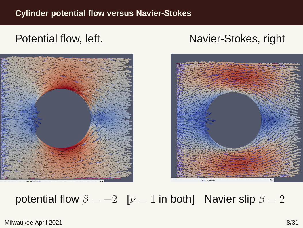
Cylinder potential flow versus Navier-Stokes


Potential flow, left. Navier-Stokes, right


New Theory of Flight


In the paper New theory of flight published in theJournal of Mathematical Fluid Mechanics in 2016,Johan Hoffman, Johan Jansson, and Claes Johnsonproposed that flight could be explained as

potential flow augmented with rotational vortices

generated at the trailing edge of a wing, which are

instabilities caused by small perturbations in the flow

We modify and clarify this slightly to suggest

• Navier friction boundary conditions with β > 0

• Reynolds-Orr kinetic instabilities.

New Theory of Flight: cylinder flow

Milwaukee April 2021 10/31Vortices generated by perturbations in incoming flow.

New Theory significant features


Main feature of new theory is that

instabilities occur at the trailing edge,

not the leading edge.

Might expect instabilities to occur at the leading edge.

Can be explained as instability caused by opposing flow.

Reynolds-Orr kinetic energy instability condition

gives precise mathematical condition and prediction.

Conventional linear stability analysis can fail completely.

Inequality versus equality


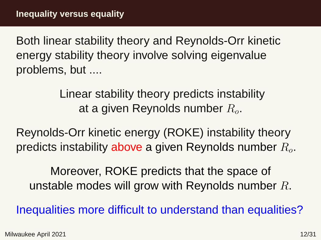
Both linear stability theory and Reynolds-Orr kineticenergy stability theory involve solving eigenvalueproblems, but ....

Linear stability theory predicts instabilityat a given Reynolds number Ro.

Reynolds-Orr kinetic energy (ROKE) instability theorypredicts instability above a given Reynolds number Ro.

Moreover, ROKE predicts that the space ofunstable modes will grow with Reynolds number R.

Inequalities more difficult to understand than equalities?

Reynolds-Orr kinetic energy instability theory


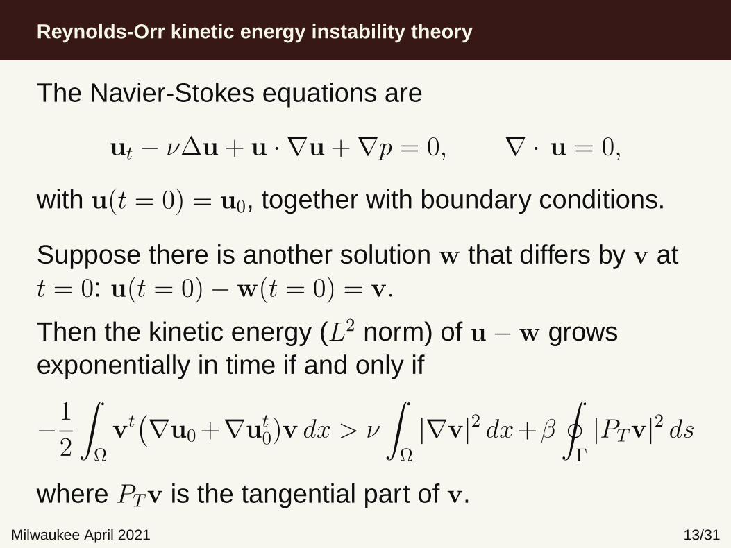
The Navier-Stokes equations are

ut − ν∆u+ u · ∇u+∇p = 0, ∇ · u = 0,

with u(t = 0) = u0, together with boundary conditions.

Suppose there is another solution w that differs by v att = 0: u(t = 0)−w(t = 0) = v.

Then the kinetic energy (L2 norm) of u−w growsexponentially in time if and only if

−1

2

∫

Ω

vt(

∇u0+∇ut0)v dx > ν

∫

Ω

|∇v|2 dx+β

∮

Γ

|PTv|2 ds

where PTv is the tangential part of v.

Reynolds-Orr eigenproblem


To determine if there is a v such that

−1

2

∫

Ω

vt(

∇u0+∇ut0)v dx > ν

∫

Ω

|∇v|2 dx+β

∮

Γ

|PTv|2 ds

consider the eigenvalue problem

λ = min1

2

∫

Ωvt(

∇u0 +∇ut0)v dx

ν∫

Ω|∇v|2 dx+ β

∮

Γ|PTv|2 ds

Then instability can occur if λ < −1

The corresponding eigenvector v gives an unstablemode.

Reynolds-Orr eigenproblem


Since ∇ · u = 0, the trace of ∇u0 +∇ut0 is zero, so it is

natural to expect that there are functions v such that∫

Ω

vt(

∇u0 +∇ut0)v dx < 0,

as well as the other sign.

For n > 1 eigenvalues less than −1, there is a space ofdimension n of unstable modes, spanned by thecorresponding eigenvectors.

Test case: Couette flow. Linear analysis says

no instabilities.

Couette flow


Couette flow [8] of interest for more than a century.

It is the simplest possible flow problem: u = Uh(y, 0).

Valid for all flow speeds U (i.e., all Reynolds numbers).

Linearly stable for all flow speeds!

Most unstable mode for Couette flow


< −−−−

−−−− >

Horizontal flow component of most unstable modeperturbation for Couette flow. Arrows indicate base flow.

Perturbation evolution

Turbulent burst for Couette flow


Re 180 200 600 1600 3K 10K 30K 100KTmax 0.44 0.52 0.89 1.01 1.06 1.13 1.20 1.36Amax 1.02 1.04 1.34 1.69 1.96 2.54 3.37 4.55TP 0.71 0.89 1.77 2.23 2.98 4.21 6.73 9.26

Table 1: Tmax is time of maximal perturbation increase Amax. TP is thepersistence time after which the perturbation stays smaller than the orignialperturbation in mean-squared gradient norm.

Perturbation evolution

Why was this missed?


Physical and computational experiments for Couetteflow indicate instability for Reynolds numberscomparable to Reynolds–Orr kinetic energy prediction.

Why was this missed for so long?

Possible answers/contributors:

• inertia of linearized stability analysis• old ways of thinking about partial differential

equations (PDEs)• Serrin focused on stability, not instability

Kinetic energy approach is natural in the variationalapproach to PDEs.

Short history of PDEs


Newton (1643–1727) and Leibnitz (1646–1716)the beginning (negative numbers considered absurd)

Euler (1707–1783)inviscid flow equations (complex numbers established)

Dirichlet (1805–1859) (Navier and Stokes)variational principle

Banach (1892–1945) and Hilbert (1862–1943)functional analysis, duality

J.-L. Lions (1928–2001) (Serrin)variational approach

Chandrasekhar — used Euler’s approach to PDEs

Failure of linear instability theory


Linear stability analysis examines a linearization ofNavier–Stokes. This is necessarily approximate.

A linearized eigenproblem is generated, but it is notsymmetric. So there are not necessarily solutions(defective).

When a solution of the linearized eigenproblem is found,it is assumed that there is a nearby solution ofNavier–Stokes.

But this assumes a stability property.

You cannot use stability to prove instability.

Why this matters


Computational simulation of aerodynamics is not in thecritical path of airplane design today.

Stall prediction beyond capability of most codes.

737 Max was considered likely to stall, leading to MCAS.

Rather than simulating the MAX to determine

likelihood of stall, MCAS was enhanced.

The rest of the story is well known.

New Theory of Flight =⇒ critical behavior computable.

MCAS = Maneuvering Characteristics Augmentation System

New Theory of Flight: cylinder

Milwaukee April 2021 23/31Can we explain voritices via ROKE instabilities?

Flow around a cylinder: most unstable mode


Stability of flow around a cylinder studied in [1].

3D instability around a cylinder: next most unstable mode


Second 2D instability


Many more instabilities as flow speed increases.

Cylinder drag: D’Alembert explained


ν = 1.0 ν = 0.1 ν = 0.01

β = 0 4.90 0.91 0.14β = 1 5.52 1.49 0.99β = 10 6.79 1.72 1.01β = 100 7.27 1.73 1.01

Table 2: Drag coefficients CD for the cylinder.

The drag force is proportional to

CD

U 2

ρ

where U is the speed and ρ is the fluid density.

Agrees well with experimental data [2, 3].

New approach to turbulence


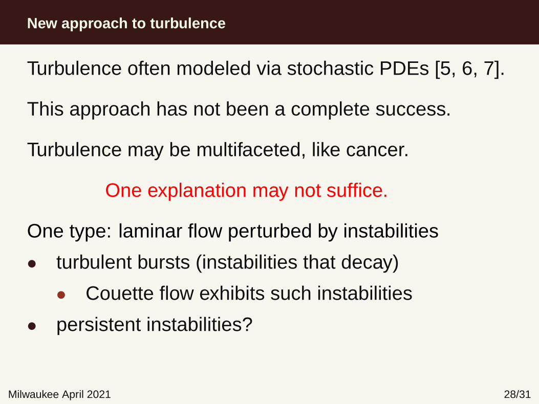
Turbulence often modeled via stochastic PDEs [5, 6, 7].

This approach has not been a complete success.

Turbulence may be multifaceted, like cancer.

One explanation may not suffice.

One type: laminar flow perturbed by instabilities

• turbulent bursts (instabilities that decay)

• Couette flow exhibits such instabilities

• persistent instabilities?

Conclusions and Implications


The New Theory of Flight holds promise to

change qualitatively fluid flow simulation.

— Use computational simulation to optimize designsand assess deficiencies.

— Improve performance of vehicles, propulsionsystems, energy generation, medical treatment.

— New way to think about turbulence.

— More realistic flight simulators for pilot training.

— Computational certification of aircraft.

Acknowledgments


We thank

• Patrick Farrell, Oxford University• Ingeborg Gjerde, Simula, Oslo• Matt Knepley, University of Buffalo• Mats Larson, Umea University• Leo Rebholz, Clemson University• Nick Trefethen, Cambridge University

for valuable suggestions.

Our understanding of this subject was enhancedsubstantially by the book [4] by Johan Hoffman andClaes Johnson.

References


[1] Ingeborg Gjerde and L. Ridgway Scott. Kinetic-energy instability of flows with slipboundary conditions. TBD, ?:??, 2021.

[2] Sydney Goldstein. Modern developments in fluid dynamics: an account of theory andexperiment relating to boundary layers, turbulent motion and wakes, volume 2.Clarendon Press, 1938.

[3] C. F. Heddleson, D. L. Brown, and R. T. Cliffe. Summary of drag coefficients of variousshaped cylinders. Technical report, General Electric Co., Cincinnati OH, 1957.

[4] Johan Hoffman and Claes Johnson. Computational Turbulent Incompressible Flow.Springer Science & Business Media, 2007.

[5] R. E. Meyers, C. Dopazo, E. E. O’Brien, and L. R. Scott. Application of probabilitydensities and intermittency to random processes in environmental chemistry andhydrodynamics. In Advances in Environmental Science and Engineering, J. R. Pfafflinand E. N. Ziegler, eds., pages 128–148. New York: Gordon and Breach, 1979.

[6] R. E. Meyers, E. E. O’Brien, and L. R. Scott. Derivation of the probability densityfunction for a stochastic nonlinear advection equation. Technical Report BNL 50732,Brookhaven National Laboratory, 1977.

[7] R. E. Meyers, E. E. O’Brien, and L. R. Scott. Random advection of chemically reactingspecies. J. Fluid Mech., 85:233–240, 1978.

[8] L. Ridgway Scott. Kinetic energy flow instability with application to Couette flow.Research Report UC/CS TR-2020-07, Dept. Comp. Sci., Univ. Chicago, 2020.

A Modern Approach to Simulating Flight

Documents

Transcript of A Modern Approach to Simulating Flight

References

Milwaukee April 2021 31/31