
A Modeling Framework for Simulating River and Stream Water ...
121
A Modeling Framework for Simulating River and Stream Water Quality Documentation and Users Manual The Mystic River at Medford, MA Steve Chapra and Greg Pelletier November 25, 2003 Chapra, S.C. and Pelletier, G.J. 2003. QUAL2K: A Modeling Framework for Simulating River and Stream Water Quality: Documentation and Users Manual. Civil and Environmental Engineering Dept., Tufts University, Medford, MA., [email protected]
Transcript of A Modeling Framework for Simulating River and Stream Water ...

A Modeling Framework for Simulating River and Stream Water Quality
Documentation and Users Manual
The Mystic River at Medford, MA
Steve Chapra and Greg Pelletier November 25, 2003 Chapra, S.C. and Pelletier, G.J. 2003. QUAL2K: A Modeling Framework for Simulating River and Stream Water Quality: Documentation and Users Manual. Civil and Environmental Engineering Dept., Tufts University, Medford, MA., [email protected]


QUAL2K 3 November 25, 2003
1 INTRODUCTION QUAL2K (or Q2K) is a river and stream water quality model that is intended to represent a modernized version of the QUAL2E (or Q2E) model (Brown and Barnwell 1987). Q2K is similar to Q2E in the following respects:
• One dimensional. The channel is well-mixed vertically and laterally. • Steady state hydraulics. Non-uniform, steady flow is simulated. • Diurnal heat budget. The heat budget and temperature are simulated as a function of
meteorology on a diurnal time scale. • Diurnal water-quality kinetics. All water quality variables are simulated on a diurnal time
scale. • Heat and mass inputs. Point and non-point loads and abstractions are simulated.
The QUAL2K framework includes the following new elements: • Software Environment and Interface. Q2K is implemented within the Microsoft Windows
environment. It is programmed in the Windows macro language: Visual Basic for Applications (VBA). Excel is used as the graphical user interface.
• Model segmentation. Q2E segments the system into river reaches comprised of equally spaced elements. In contrast, Q2K uses unequally-spaced reaches. In addition, multiple loadings and abstractions can be input to any reach.
• Carbonaceous BOD speciation. Q2K uses two forms of carbonaceous BOD to represent organic carbon. These forms are a slowly oxidizing form (slow CBOD) and a rapidly oxidizing form (fast CBOD). In addition, non-living particulate organic matter (detritus) is simulated. This detrital material is composed of particulate carbon, nitrogen and phosphorus in a fixed stoichiometry.
• Anoxia. Q2K accommodates anoxia by reducing oxidation reactions to zero at low oxygen levels. In addition, denitrification is modeled as a first-order reaction that becomes pronounced at low oxygen concentrations.
• Sediment-water interactions. Sediment-water fluxes of dissolved oxygen and nutrients are simulated internally rather than being prescribed. That is, oxygen (SOD) and nutrient fluxes are simulated as a function of settling particulate organic matter, reactions within the sediments, and the concentrations of soluble forms in the overlying waters.
• Bottom algae. The model explicitly simulates attached bottom algae. • Light extinction. Light extinction is calculated as a function of algae, detritus and
inorganic solids. • pH. Both alkalinity and total inorganic carbon are simulated. The river’s pH is then
simulated based on these two quantities. • Pathogens. A generic pathogen is simulated. Pathogen removal is determined as a
function of temperature, light, and settling.


QUAL2K 5 November 25, 2003
2 GETTING STARTED Installation is required for many water-quality models. This is not the case for QUAL2K because the model is packaged as an Excel Workbook. The program is written in Excel’s macro language: Visual Basic for Applications or VBA. The Excel Workbook’s worksheets and charts are used to enter data and display results. Consequently, you merely have to open the Workbook to begin modeling. The following are some recommended step-by-step instructions on how to obtain your first model run. Step 1: Create a folder named QUAL2K to hold the workbook and its data files. For example, in the following example, a folder named QUAL2K is created on the C:\ drive. Step 2: Copy the Q2KMaster file (Q2KMaster.xls) from your CD to C:\QUAL2K. Step 3: Open Excel and make sure that your macro security level is set to medium (Figure 1). This can be done using the menu commands: Tools → Macro → Security. Make certain that the Medium radio button is selected.
Figure 1 The Excel Macro Security Level dialogue box. In order to run Q2K, the Medium level of security should be selected.
Step 4: Open Q2KMaster.xls. When you do this, the Macro Security Dialogue Box will be displayed (Figure 2).
QUAL2K 6 November 25, 2003
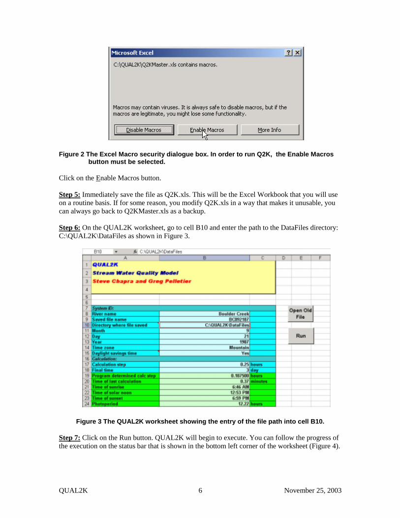
Figure 2 The Excel Macro security dialogue box. In order to run Q2K, the Enable Macros button must be selected.
Click on the Enable Macros button. Step 5: Immediately save the file as Q2K.xls. This will be the Excel Workbook that you will use on a routine basis. If for some reason, you modify Q2K.xls in a way that makes it unusable, you can always go back to Q2KMaster.xls as a backup. Step 6: On the QUAL2K worksheet, go to cell B10 and enter the path to the DataFiles directory: C:\QUAL2K\DataFiles as shown in Figure 3.
Figure 3 The QUAL2K worksheet showing the entry of the file path into cell B10. Step 7: Click on the Run button. QUAL2K will begin to execute. You can follow the progress of the execution on the status bar that is shown in the bottom left corner of the worksheet (Figure 4).

QUAL2K 7 November 25, 2003
Figure 4 The QUAL2K Status Bar is positioned at the lower left corner of the worksheet. It allows you to follow the progress of a model run.
If the program runs properly, the temperature plot will be displayed. If it does not work
properly, two possibilities exist: First, you may be using an old version of Microsoft Office. Although Excel is downwardly
compatible for some earlier versions, Q2K will not work with very old versions. Second, you may have made a mistake in implementing the preceding steps. A common
mistake is to have mistyped the file path that you entered in cell B10. If this is the case, you will receive an error message (Figure 5).
Figure 5 An error message that will occur if you type the incorrect file path into cell B10 on the QUAL2K worksheet.
If this occurs, click on the end button. This will terminate the run and bring you back to the
Excel Workbook. You should then move back to the QUAL2K worksheet and correct the file path entry. Note that the same error will occur if you did not set up your directories with correct names as specified above. Step 8: On the QUAL2K worksheet click on the Open Old File button. Browse to get to the directory: C:\QUAL2K\DataFiles. You should see that a new file: BC092187.q2k has been created. Click on the Cancel button to return to Q2K.
Note that every time that Q2K is run, a data file will be created with the file name specified in cell B9 on the QUAL2K worksheet (Figure 3). The program automatically affixes the extension .q2k to the file name. Since this will overwrite the file, make certain to change the file name when you perform a new application.


QUAL2K 9 November 25, 2003
3 SEGMENTATION AND HYDRAULICS The model presently simulates the main stem of a river as depicted in Figure 6. Tributaries are not modeled explicitly, but can be represented as point sources.
1
2
3
456
8
7
Non-pointabstraction
Non-pointsource
Point source
Point source
Point abstractionPoint abstraction
Headwater boundary
Downstream boundary
Point source
Figure 6 QUAL2K segmentation scheme.
3.1 Flow Balance A steady-state flow balance is implemented for each model reach (Figure 7)
iabiinii QQQQ ,,1 −+= − (1)
where Qi = outflow from reach i into reach i + 1 [m3/d], Qi–1 = inflow from the upstream reach i – 1 [m3/d], Qin,i is the total inflow into the reach from point and nonpoint sources [m3/d], and Qab,i is the total outflow from the reach due to point and nonpoint abstractions [m3/d].
i i + 1i −−−− 1Qi−−−−1 Qi
Qin,i Qab,i
Figure 7 Reach flow balance.

QUAL2K 10 November 25, 2003
The total inflow from sources is computed as
∑∑==
+=npsi
jjinps
psi
jjipsiin QQQ
1,,
1,,, (2)
where Qps,i,j is the jth point source inflow to reach i [m3/d], psi = the total number of point sources to reach i, Qnps,i,j is the jth non-point source inflow to reach i [m3/d], and npsi = the total number of non-point source inflows to reach i.
The total outflow from abstractions is computed as
∑∑==
+=npai
jjinpa
pai
jjipaiab QQQ
1,,
1,,, (3)
where Qpa,i,j is the jth point abstraction outflow from reach i [m3/d], pai = the total number of point abstractions from reach i, Qnpa,i,j is the jth non-point abstraction outflow from reach i [m3/d], and npai = the total number of non-point abstraction flows from reach i.
The non-point sources and abstractions are modeled as line sources. As in Figure 8, the non-point source or abstraction is demarcated by its starting and ending kilometer points. Its flow is distributed to or from each reach in a length-weighted fashion.
Qnpt
25%Qnpt 25%Qnpt 50%Qnpt
start end
Figure 8 The manner in which non-point source flow is distributed to a reach.
3.2 Hydraulic Characteristics Once the outflow for each reach is computed, the depth and velocity are calculated in one of three ways: weirs, rating curves, and Manning equations. The program decides among these options in the following manner:
• If a weir height is entered, the weir option is implemented.
QUAL2K 11 November 25, 2003
• If the weir height is zero and a roughness coefficient is entered (n), the Manning equation option is implemented.
• If neither of the previous conditions are met, Q2K uses rating curves.
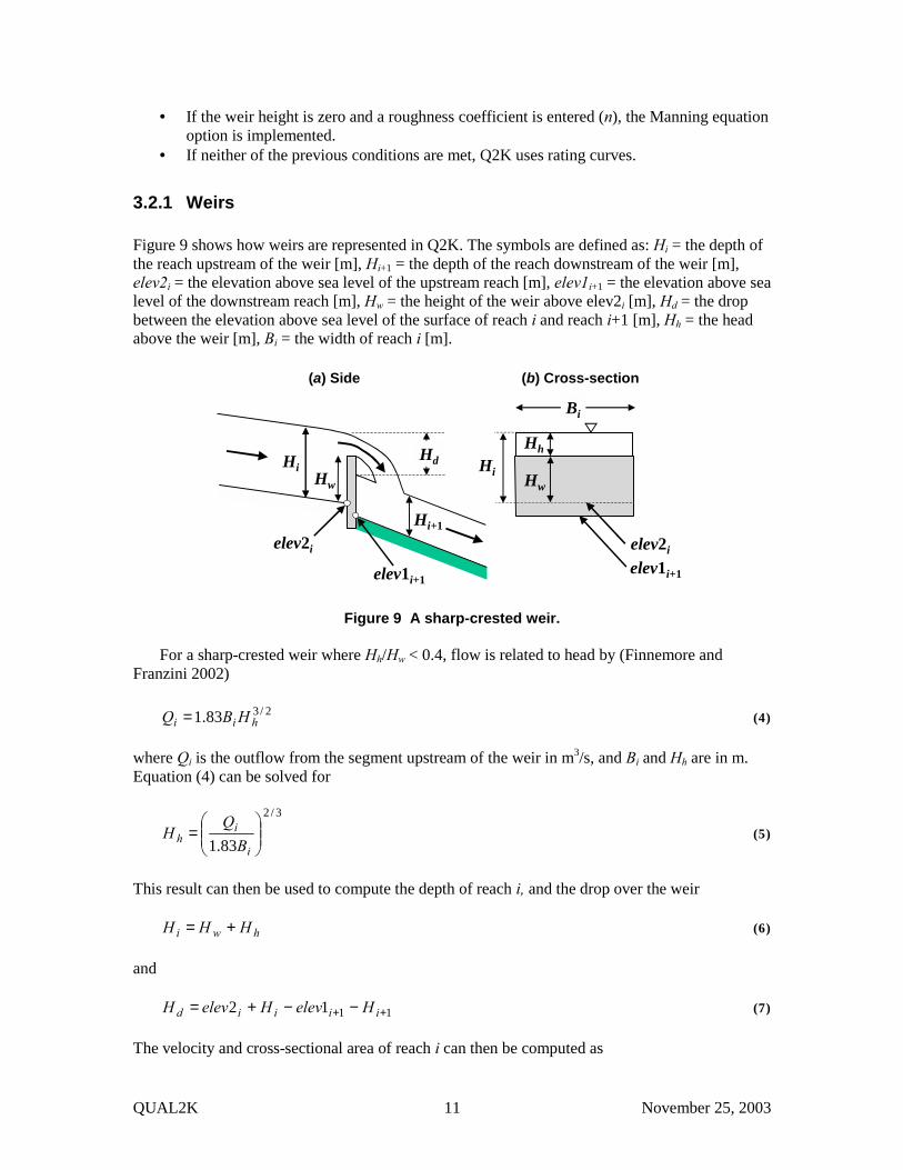
3.2.1 Weirs Figure 9 shows how weirs are represented in Q2K. The symbols are defined as: Hi = the depth of the reach upstream of the weir [m], Hi+1 = the depth of the reach downstream of the weir [m], elev2i = the elevation above sea level of the upstream reach [m], elev1i+1 = the elevation above sea level of the downstream reach [m], Hw = the height of the weir above elev2i [m], Hd = the drop between the elevation above sea level of the surface of reach i and reach i+1 [m], Hh = the head above the weir [m], Bi = the width of reach i [m].
Hi+1
Hw
Hi
Bi
Hd
(a) Side (b) Cross-section
HwHi
Hh
elev2i
elev1i+1
elev2i
elev1i+1
Figure 9 A sharp-crested weir.
For a sharp-crested weir where Hh/Hw < 0.4, flow is related to head by (Finnemore and Franzini 2002)
2/383.1 hii HBQ = (4)
where Qi is the outflow from the segment upstream of the weir in m3/s, and Bi and Hh are in m. Equation (4) can be solved for
3/2
83.1
=
i
ih B
QH (5)
This result can then be used to compute the depth of reach i, and the drop over the weir
hwi HHH += (6)
and
1112 ++ −−+= iiiid HelevHelevH (7)
The velocity and cross-sectional area of reach i can then be computed as

QUAL2K 12 November 25, 2003
iiic HBA =, (8)
ic
ii A
QU
,= (9)
3.2.2 Rating Curves Power equations can be used to relate mean velocity and depth to flow,
baQU = (10)
βαQH = (11)
where a, b, α and β are empirical coefficients that are determined from velocity-discharge and stage-discharge rating curves, respectively. The values of velocity and depth can then be employed to determine the cross-sectional area and width by
UQAc = (12)
HA
B c= (13)
The exponents b and β typically take on values listed in Table 1. Note that the sum of b and β
must be less than or equal to 1. If their sum equals 1, the channel is rectangular.
Table 1 Typical values for the exponents of rating curves used to determine velocity and depth from flow (Barnwell et al. 1989).
Equation Exponent Typical value Range
baQU = b 0.43 0.4−0.6
H Q=α β β
0.45 0.3−0.5
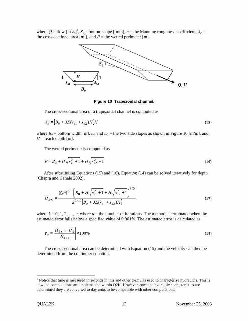
3.2.3 Manning Equation Each reach is idealized as a trapezoidal channel (Figure 10). Under conditions of steady flow, the Manning equation can be used to express the relationship between flow and depth as
3/2
3/52/10
PA
nSQ c= (14)
QUAL2K 13 November 25, 2003
where Q = flow [m3/s]1, S0 = bottom slope [m/m], n = the Manning roughness coefficient, Ac = the cross-sectional area [m2], and P = the wetted perimeter [m].
Q, UB0
1 1ss1 ss2
H
S0
Figure 10 Trapezoidal channel.
The cross-sectional area of a trapezoidal channel is computed as
[ ]HHssBA ssc )(5.0 210 ++= (15)
where B0 = bottom width [m], ss1 and ss2 = the two side slopes as shown in Figure 10 [m/m], and H = reach depth [m].
The wetted perimeter is computed as
11 22
210 ++++= ss sHsHBP (16)
After substituting Equations (15) and (16), Equation (14) can be solved iteratively for depth
(Chapra and Canale 2002),
[ ]HssBS
sHsHBQnH
ss
ss
k)(5.0
11)(
21010/3
5/222
210
5/3
1++
++++
=+ (17)
where k = 0, 1, 2, …, n, where n = the number of iterations. The method is terminated when the estimated error falls below a specified value of 0.001%. The estimated error is calculated as
%1001
1 ×−
=+
+
k
kka H
HHε (18)
The cross-sectional area can be determined with Equation (15) and the velocity can then be
determined from the continuity equation,
1 Notice that time is measured in seconds in this and other formulas used to characterize hydraulics. This is how the computations are implemented within Q2K. However, once the hydraulic characteristics are determined they are converted to day units to be compatible with other computations.

QUAL2K 14 November 25, 2003
cAQU = (19)
The average reach width, B [m], can be computed as
HA
B c= (20)
Suggested values for the Manning coefficient are listed in Table 2.
Table 2 The Manning roughness coefficient for various open channel surfaces (from Chow
et al. 1988).
MATERIAL n Man-made channels Concrete 0.012 Gravel bottom with sides:
concrete 0.020 mortared stone 0.023 riprap 0.033
Natural stream channels Clean, straight 0.025-0.04 Clean, winding and some weeds 0.03-0.05 Weeds and pools, winding 0.05 Mountain streams with boulders 0.04-0.10 Heavy brush, timber 0.05-0.20
Manning’s n typically varies with flow and depth (Gordon et al, 1992). As the depth
decreases at low flow, the relative roughness increases. Typical published values of Manning’s n, which range from about 0.015 for smooth channels to about 0.15 for rough natural channels, are representative of conditions when the flow is at the bankfull capacity (Rosgen, 1996). Critical conditions of depth for evaluating water quality are generally much less than bankfull depth, and the relative roughness may be much higher.
3.2.4 Waterfalls
In Section 3.2.1, the drop of water over a weir was computed. This value is needed in order to compute the enhanced reaeration that occurs in such cases. In addition to weirs, such drops can also occur at waterfalls (Figure 11).

QUAL2K 15 November 25, 2003
Hi+1
HiHd
elev2i
elev1i+1
Figure 11 Waterfall.
QUAL2K computes such drops for cases where the elevation above sea level drops abruptly at the boundary between two reaches. For both the rating curve and the Manning equation options, the model uses Equation (7) for this purpose. It should be noted that the drop is only calculated when the elevation above sea level at the downstream end of a reach is greater than at the beginning of the next downstream reach; that is, elev2i > elev1i+1.
3.3 Travel Time The residence time of each reach is computed as
k
kk Q
V=τ (21)
where τk = the residence time of the kth reach [d], Vk = the volume of the kth reach [m3] = Ac,k∆xk, and ∆xk = the length of the kth reach [m]. These times are then accumulated to determine the travel time from the headwater to the downstream end of reach i,
∑=
=i
kkitt
1, τ (22)
where tt,i = the travel time [d].
∑=
=
=
i
kkit
k
kk
t
QV
1, τ
τ
3.4 Longitudinal Dispersion
QUAL2K 16 November 25, 2003
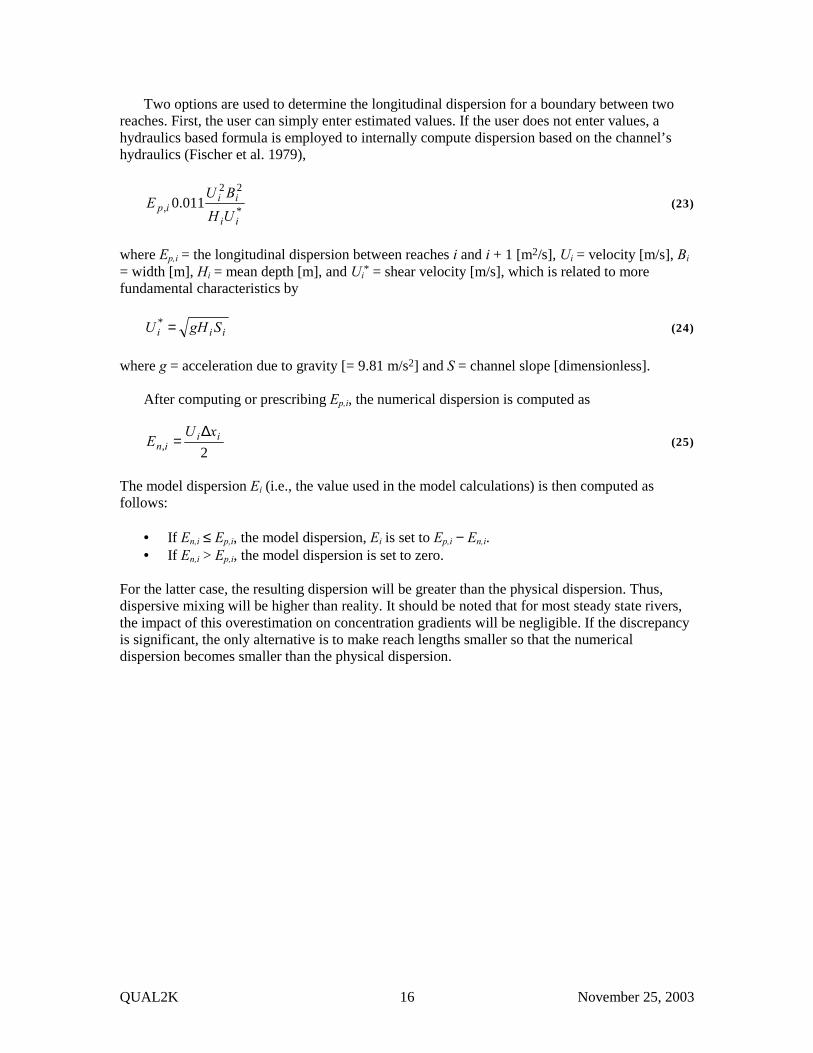
Two options are used to determine the longitudinal dispersion for a boundary between two reaches. First, the user can simply enter estimated values. If the user does not enter values, a hydraulics based formula is employed to internally compute dispersion based on the channel’s hydraulics (Fischer et al. 1979),
*
22
, 011.0ii
iiip
UHBU
E (23)
where Ep,i = the longitudinal dispersion between reaches i and i + 1 [m2/s], Ui = velocity [m/s], Bi = width [m], Hi = mean depth [m], and Ui* = shear velocity [m/s], which is related to more fundamental characteristics by
iii SgHU =* (24) where g = acceleration due to gravity [= 9.81 m/s2] and S = channel slope [dimensionless].
After computing or prescribing Ep,i, the numerical dispersion is computed as
2,ii
inxU
E∆
= (25)
The model dispersion Ei (i.e., the value used in the model calculations) is then computed as follows:
• If En,i ≤ Ep,i, the model dispersion, Ei is set to Ep,i − En,i. • If En,i > Ep,i, the model dispersion is set to zero.
For the latter case, the resulting dispersion will be greater than the physical dispersion. Thus, dispersive mixing will be higher than reality. It should be noted that for most steady state rivers, the impact of this overestimation on concentration gradients will be negligible. If the discrepancy is significant, the only alternative is to make reach lengths smaller so that the numerical dispersion becomes smaller than the physical dispersion.

QUAL2K 17 November 25, 2003
4 TEMPERATURE MODEL As in Figure 12, the heat balance takes into account heat transfers from adjacent reaches, loads, abstractions, the atmosphere, and the sediments. A heat balance can be written for reach i as
( ) ( )
+
+
+
−+−+−−= +−−
−−
cm 100m
cm 100m
cm 10m ,,
36
3,
1
'
1
'1,
11
ipww
is
ipww
ih
ipww
ih
iii
iii
i
ii
i
iabi
i
ii
i
ii
HCJ
HCJ
VCW
TTVE
TTV
ET
VQ
TVQ
TV
Qdt
dT
ρρρ
(26)
where Ti = temperature in reach i [oC], t = time [d], E’i = the bulk dispersion coefficient between reaches i and i + 1 [m3/d], Wh,i = the net heat load from point and non-point sources into reach i [cal/d], ρw = the density of water [g/cm3], Cpw = the specific heat of water [cal/(g oC)], Jh,i = the air-water heat flux [cal/(cm2 d)], and Js,i = the sediment-water heat flux [cal/(cm2 d)].
iinflow outflow
dispersion dispersion
heat load heat abstraction
atmospherictransfer
sediment-watertransfer
sediment
Figure 12 Heat balance.
The bulk dispersion coefficient is computed as
( ) 2/1
,'
+∆+∆=
ii
icii xx
AEE (27)
Note that a zero dispersion condition is applied at the downstream boundary.
The net heat load from sources is computed as
+= ∑∑
==
npsi
jjnpsijinps
psi
jjpsijipspih TQTQCW
1,,,
1,,,, ρ (28)

QUAL2K 18 November 25, 2003
where Tps,i,j is the jth point source temperature for reach i [oC], and Tnps,i,j is the jth non-point source temperature for reach i [oC].
4.1 Surface Heat Flux As depicted in Figure 13, surface heat exchange is modeled as a combination of five processes:
ecbranh JJJJIJ −−−+= )0( (29)
where I(0) = net solar shortwave radiation at the water surface, Jan = net atmospheric longwave radiation, Jbr = longwave back radiation from the water, Jc = conduction, and Je = evaporation. All fluxes are expressed as cal/cm2/d.
air-waterinterface
solarshortwaveradiation
atmosphericlongwaveradiation
waterlongwaveradiation
conductionand
convection
evaporationand
condensation
radiation terms non-radiation terms
net absorbed radiation water-dependent terms
Figure 13 The components of surface heat exchange.
4.1.1 Solar Radiation The model computes the amount of solar radiation entering the water at a particular latitude (Lat) and longitude (Llm) on the earth’s surface. This quantity is a function of the radiation at the top of the earth’s atmosphere which is attenuated by atmospheric transmission, cloud cover, shade, and reflection,
nattenuation attenuatio radiation shading reflection cloud catmospheri strialextraterre
)1( )1( )0( 0 fsct SRaaII −−= (30)
where I(0) = solar radiation at the water surface [cal/cm2/d], I0 = extraterrestrial radiation (i.e., at the top of the earth’s atmosphere) [cal/cm2/d], at = atmospheric attenuation, CL = fraction of sky covered with clouds, Rs = albedo (fraction reflected), and Sf = effective shade (fraction blocked by vegetation and topography).
Extraterrestrial radiation. The extraterrestrial radiation is computed as (TVA 1972)

QUAL2K 19 November 25, 2003
αsin20
0rW
I = (31)
where W0 = the solar constant [1367 W/m2 or 2823 cal/cm2/d], r = normalized radius of the earth’s orbit (i.e., the ratio of actual earth-sun distance to mean earth-sun distance), and α = the sun’s altitude [radians], which can be computed as
( )τδδα coscoscossinsinsin atat LL += (32)
where δ = solar declination [radians], Lat = local latitude [radians], and τ = the local hour angle of the sun [radians].
The normalized radius can be estimated as
−+= )186(3652cos017.01 Dyr π (33)
where Dy = Julian day (Jan. 1 = 1, Jan. 2 = 2, etc.).
The solar declination can be estimated as
−= )172(3652cos
18045.23 Dyππδ (34)
The local hour angle in radians is given by
180180
4πτ
−= imetrueSolarT (35)
where:
timezoneLeqtimelocalTimeimetrueSolarT lm ×−×−+= 604 (36)
where trueSolarTime is the solar time determined from the actual position of the sun in the sky [minutes], localTime is the local time in minutes (local standard time), Llm is the local longitude (positive decimal degrees for the western hemisphere), and timezone is the local time zone in hours relative to Greenwich Mean Time (e.g. -8 hours for Pacific Standard Time; the local time zone is selected on the Qual2K worksheet). The value of eqtime represents the difference between true solar time and mean solar time in minutes of time.
QUAL2K calculates the sun’s altitude and eqtime, as well as the times of sunrise and sunset using the Meeus (1999) algorithms as implemented by NOAA’s Surface Radiation Research Branch (www.srrb.noaa.gov/highlights/sunrise/azel.html). The NOAA method for solar position that is used in QUAL2K also includes a correction for the effect of atmospheric refraction. The complete calculation method that is used to determine the solar position, eqtime, sunrise and sunset is presented in Appendix 2.
The photoperiod f [hours] is computed as

QUAL2K 20 November 25, 2003
srss ttf −= (37)
where tss = time of sunset [hours] and tsr = time of sunrise [hours]. Atmospheric attenuation. Various methods have been published to estimate the fraction of the atmospheric attenuation from a clear sky (at). Two alternative methods are available in QUAL2K to estimate at:
• Bras (1990) • Ryan and Stolzenbach (1972)
Note that the solar radiation model is selected on the Light and Heat worksheet of QUAL2K.
The Bras (1990) method computes at as:
mant
facea 1−= (38)
where nfac is an atmospheric turbidity factor that varies from approximately 2 for clear skies to 4 or 5 for smoggy urban areas. The molecular scattering coefficient (a1) is calculated as
ma 101 log054.0128.0 −= (39)
where m is the optical air mass, calculated as
253.1)885.3(15.0sin1
−++=
dm
αα (40)
where αd is the sun’s altitude in degrees from the horizon = α × (180o/π).
The Ryan and Stolzenbach (1972) model computes at from ground surface elevation and solar altitude as:
256.5
2880065.0288
−=
elevmtct aa (41)
where atc is the atmospheric transmission coefficient (0.70-0.91, typically approximately 0.8), and elev is the ground surface elevation in meters.
Direct measurements of solar radiation are available at some locations. For example, NOAA’s Integrated Surface Irradiance Study (ISIS) has data from various stations across the United States (http://www.atdd.noaa.gov/isis.htm). The selection of either the Bras or Ryan-Stolzenbach solar radiation model and the appropriate atmospheric turbidity factor or atmospheric transmission coefficient for a particular application should ideally be guided by a comparison of predicted solar radiation with measured values at a reference location. Cloud Attenuation. Attenuation of solar radiation due to cloud cover is computed with

QUAL2K 21 November 25, 2003
265.01 Lc Ca −= (42)
where CL = fraction of the sky covered with clouds. Reflectivity. Reflectivity is calculated as
Bds AR α= (43)
where A and B are coefficients related to cloud cover (Table 3).
Table 3 Coefficients used to calculate reflectivity based on cloud cover.
Cloudiness Clear Scattered Broken Overcast CL 0 0.1-0.5 0.5-0.9 1.0 Coefficients A B A B A B A B 1.18 −0.77 2.20 −0.97 0.95 −0.75 0.35 −0.45 Shade. Shade is an input variable for the QUAL2K model. Shade is defined as the fraction of potential solar radiation that is blocked by topography and vegetation. An Excel/VBA program named ‘Shade.xls’ is available from the Washington Department of Ecology to estimate shade from topography and riparian vegetation (Ecology 2003). Input values of integrated hourly estimates of shade are put into the Shade worksheet of QUAL2K.
4.1.2 Atmospheric Long-wave Radiation The downward flux of longwave radiation from the atmosphere is one of the largest terms in the surface heat balance. This flux can be calculated using the Stefan-Boltzmann law
( ) ( )Lskyairan RTJ −+= 1 273 4 εσ (44)
where σ = the Stefan-Boltzmann constant = 11.7x10⁻⁸ cal/(cm2 d K4), Tair = air temperature [oC], εsky = effective emissivity of the atmosphere [dimensionless], and RL = longwave reflection coefficient [dimensionless]. Emissivity is the ratio of the longwave radiation from an object compared with the radiation from a perfect emitter at the same temperature. The reflection coefficient is generally small and in typically assumed to equal 0.03.
The atmospheric longwave radiation model is selected on the Light and Heat worksheet of QUAL2K. Three alternative methods are available for use in QUAL2K to represent the effective emissivity (εsky): Brutsaert (1982). The Brutsaert equation is physically-based instead of empirically derived and has been shown to yield satisfactory results over a wide range of atmospheric conditions of air temperature and humidity at intermediate latitudes for conditions above freezing (Brutsaert, 1982).
7/1333224.1
24.1
=
a
airclear T
eε

QUAL2K 22 November 25, 2003
where eair is the air vapor pressure [mm Hg], and Ta is the air temperature in °K. The factor of 1.333224 converts the vapor pressure from mm Hg to millibars. The air vapor pressure [in mm Hg] is computed as (Raudkivi 1979):
d
d
TT
air ee += 3.23727.17
596.4 (45)
where Td = the dew-point temperature [oC]. Brunt (1932). Brunt’s equation is an empirical model that has been commonly used in water-quality models (Thomann and Mueller 1987),
airbaclear eAA += ε where Aa and Ab are empirical coefficients. Values of Aa have been reported to range from about 0.5 to 0.7 and values of Ab have been reported to range from about 0.031 to 0.076 mmHg-0.5 for a wide range of atmospheric conditions. QUAL2K uses a default mid-range value of Aa = 0.6 with Ab = 0.031 mmHg-0.5 if the Brunt method is selected on the Light and Heat worksheet. Koberg (1964). Koberg (1964) reported that the Aa in Brunt’s formula depends on both air temperature and the ratio of the incident solar radiation to the clear-sky radiation (Rsc). As in Figure 14, he presented a series of curves indicating that Aa increases with Tair and decreases with Rsc with Ab held constant at 0.0263 millibars-0.5 (about 0.031 mmHg-0.5).
The following polynomial is used in Q2K to provide a continuous approximation of Koberg’s
curves.
kairkairka cTbTaA ++= 2
where
0.0001106 0.000730870.00121134 0.00076437 23 +−+−= scscsck RRRa
0.02586655 0.13397992 0.2204455 0.12796842 23 −+−= scscsck RRRb
1.43052757 3.43402413 5.65909609 3.25272249 23 +−+−= scscsck RRRc
The fit of this polynomial to points sampled from Koberg’s curves are depicted in Figure 14. Note that an upper limit of 0.735 is prescribed for Aa.

QUAL2K 23 November 25, 2003
0.3
0.4
0.5
0.6
0.7
0.8
-4 0 4 8 12 16 20 24 28 320.3
0.4
0.5
0.6
0.7
0.8
-4 0 4 8 12 16 20 24 28 32
Kob
erg’
s “A
a” c
onst
ant f
orB
runt
’s e
quat
ion
for l
ongw
ave
radi
atio
n
Air temperature Tair (oC)
0.95
0.90
0.850.800.750.650.50
1.00
Ratio of incident to clear sky radiation Rsc
Figure 14 The points are sampled from Koberg’s family of curves for determining the value of the Aa constant in Brunt’s equation for atmospheric longwave radiation (Koberg, 1964). The lines are the functional representation used in Q2K.
For cloudy conditions the atmospheric emissivity may increase as a result of increased water
vapor content. High cirrus clouds may have a negligible effect on atmospheric emissivity, but lower stratus and cumulus clouds may have a significant effect. The Koberg method accounts for the effect of clouds on the emissivity of longwave radiation in the determination of the Aa coefficient. The Brunt and Brutsaert methods determine emissivity of a clear sky and do not account for the effect of clouds. Therefore, if the Brunt or Brutsaert methods are selected, then the effective atmospheric emissivity for cloudy skies (εsky) is estimated from the clear sky emissivity by using a nonlinear function of the fractional cloud cover (CL) of the form (TVA, 1972):
)17.01( 2Lclearsky C+= εε (46)
The selection of the longwave model for a particular application should ideally be guided by
a comparison of predicted results with measured values at a reference location. However, direct measurements are rarely collected. The Brutsaert method is recommended to represent a wide range of atmospheric conditions.
4.1.3 Water Long-wave Radiation The back radiation from the water surface is represented by the Stefan-Boltzmann law,
( )4273+= TJ br εσ (47) where ε = emissivity of water (= 0.97) and T = the water temperature [oC].

QUAL2K 24 November 25, 2003
4.1.4 Conduction and Convection Conduction is the transfer of heat from molecule to molecule when matter of different temperatures are brought into contact. Convection is heat transfer that occurs due to mass movement of fluids. Both can occur at the air-water interface and can be described by,
( )( )airswc TTUfcJ −= 1 (48)
where c1 = Bowen's coefficient (= 0.47 mmHg/oC). The term, f(Uw), defines the dependence of the transfer on wind velocity over the water surface where Uw is the wind speed measured a fixed distance above the water surface.
Many relationships exist to define the wind dependence. Bras (1990), Edinger et al (1974),
and Shanahan (1984) provide reviews of various methods. Some researchers have proposed that conduction/convection and evaporation are negligible in the absence of wind (e.g. Marciano and Harbeck, 1952), which is consistent with the assumption that only molecular processes contribute to the transfer of mass and heat without wind (Edinger et al 1974). Others have shown that significant conduction/convection and evaporation can occur in the absence of wind (e.g. Brady Graves and Geyer 1969, Harbeck 1962, Ryan and Harleman 1971, Helfrich et al 1982, and Adams et al 1987). This latter opinion has gained favor (Edinger et al, 1974), especially for waterbodies that exhibit water temperatures that are greater than the air temperature.
Brady, Graves, and Geyer (1969) pointed out that if the water surface temperature is warmer than the air temperature, then “the air adjacent to the water surface would tend to become both warmer and more moist than that above it, thereby (due to both of these factors) becoming less dense. The resulting vertical convective air currents … might be expected to achieve much higher rates of heat and mass transfer from the water surface [even in the absence of wind] than would be possible by molecular diffusion alone” (Edinger et al, 1974). Water temperatures in natural waterbodies are frequently greater than the air temperature, especially at night.
Edinger et al (1974) recommend that the relationship that was proposed by Brady, Graves and Geyer (1969) based on data from cooling ponds, could be representative of most environmental conditions. Shanahan (1984) recommends that the Lake Hefner equation (Marciano and Harbeck, 1952) is appropriate for natural waters in which the water temperature is less than the air temperature. Shanahan also recommends that the Ryan and Harleman (1971) equation as recalibrated by Helfrich et al (1982) is best suited for waterbodies that experience water temperatures that are greater than the air temperature. Adams et al (1987) revisited the Ryan and Harleman and Helfrich et al models and proposed another recalibration using additional data for waterbodies that exhibit water temperatures that are greater than the air temperature.
Three options are available on the Light and Heat worksheet in QUAL2K to calculate f(Uw): Brady, Graves, and Geyer (1969)
295.00.19)( ww UUf +=
where Uw = wind speed at a height of 7 m [m/s].
Adams et al. (1987)

QUAL2K 25 November 25, 2003
Adams et al. (1987) updated the work of Ryan and Harleman (1971) and Helfrich et al (1982) to derive an empirical model of the wind speed function for heated waters that accounts for the enhancement of convection currents when the virtual temperature difference between the water and air (∆θv in degrees F) is greater than zero. Two wind functions reported by Adams et al., also known as the East Mesa method, are implemented in QUAL2K (wind speed in these equations is at a height of 2m).
• Adams 1: This formulation uses an empirical function to estimate effect of convection
currents caused by virtual temperature differences between water and air, and the Harbeck (1962) equation is used to represent the contribution to conduction/convection and evaporation that is not due to convection currents caused by high virtual water temperature.
2
,05.0
,23/1 )2.24()4.22(271.0)( mphwiacresvw UAUf −+∆= θ
where Uw,mph is wind speed in mph and Aacres,i is surface area of reach i in acres. The constant 0.271 converts the original units of BTU ft−2 day−1 mmHg−1 to cal cm−2 day−1 mmHg−1.
• Adams 2: This formulation uses an empirical function of virtual temperature differences
with the Marciano and Harbeck (1952) equation for the contribution to conduction/convection and evaporation that is not due to the high virtual water temperature
2
,23/1 )17()4.22(271.0)( mphwvw UUf +∆= θ
Virtual temperature is defined as the temperature of dry air that has the same density as air
under the in situ conditions of humidity. The virtual temperature difference between the water and air ( vθ∆ in °F) accounts for the buoyancy of the moist air above a heated water surface. The virtual temperature difference is estimated from water temperature (Tw,f in °F), air temperature (Tair,f in °F), vapor pressure of water and air (es and eair in mmHg), and the atmospheric pressure (patm is estimated as standard atmospheric pressure of 760 mmHg in QUAL2K):
−
++
−
−
++
=∆ 460/378.01
460460
/378.01460 ,,
atmair
fair
atms
fwv pe
Tpe
Tθ (49)
The height of wind speed measurements is also an important consideration for estimating
conduction/convection and evaporation. QUAL2K internally adjusts the wind speed to the correct height for the wind function that is selected on the Light and Heat worksheet. The input values for wind speed on the Wind Speed worksheet in QUAL2K are assumed to be representative of conditions at a height of 7 meters above the water surface. To convert wind speed measurements (Uw,z in m/s) taken at any height (zw in meters) to the equivalent conditions at a height of 7 m for input to the Wind Speed worksheet of QUAL2K, the exponential wind law equation may be used (TVA, 1972):

QUAL2K 26 November 25, 2003
15.0
=
wwzw z
zUU (50)
For example, if wind speed data were collected from a height of 2 m, then the wind speed at 7
m for input to the Wind Speed worksheet of QUAL2K would be estimated by multiplying the measured wind speed by a factor of 1.2.
4.1.5 Evaporation and Condensation The heat loss due to evaporation can be represented by Dalton’s law,
))(( airswe eeUfJ −= (51)
where es = the saturation vapor pressure at the water surface [mmHg], and eair = the air vapor pressure [mmHg]. The saturation vapor pressure is computed as
TT
air ee += 3.23727.17
596.4 (52)
4.2 Sediment-Water Heat Transfer A heat balance for bottom sediment underlying a water reach i can be written as
isedpss
isis
HCJ
dtdT
,
,,
ρ−= (53)
where Ts,i = the temperature of the bottom sediment below reach i [oC], ρs = the density of the sediments [g/cm3], Cps = the specific heat of the sediments [cal/(g oC)], Jh,i = the air-water heat flux [cal/(cm2 d)], and Js,i = the sediment-water heat flux [cal/(cm2 d)]. and Hsed,i = the effective thickness of the sediment layer [cm].
The flux from the sediments to the water can be computed as
( )isiised
spssis TT
HCJ −=
2/,,
αρ (54)
where αs = the sediment thermal diffusivity [cm2/s].
The thermal properties of some natural sediments along with its components are summarized in Table 4. Note that soft, gelatinous sediments found in the deposition zones of lakes are very porous and approach the values for water. Some very slow, impounded rivers may approach such a state. However, rivers will tend to have coarser sediments with significant fractions of sands, gravels and stones. Upland streams can have bottoms that are dominated by boulders and rock substrates.

QUAL2K 27 November 25, 2003
Table 4 Thermal properties for natural sediments and the materials that comprise natural
sediments.
Table 4. Thermal properties of various materials
Type of material ρ C p ρCp referencew/m/°C cal/s/cm/°C m2/s cm2/s g/cm3 cal/(g °C) cal/(cm^3 °C)
Sediment samplesMud Flat 1.82 0.0044 4.80E-07 0.0048 0.906 (1)Sand 2.50 0.0060 7.90E-07 0.0079 0.757 "Mud Sand 1.80 0.0043 5.10E-07 0.0051 0.844 "Mud 1.70 0.0041 4.50E-07 0.0045 0.903 "Wet Sand 1.67 0.0040 7.00E-07 0.0070 0.570 (2)Sand 23% saturation with water 1.82 0.0044 1.26E-06 0.0126 0.345 (3)Wet Peat 0.36 0.0009 1.20E-07 0.0012 0.717 (2)Rock 1.76 0.0042 1.18E-06 0.0118 0.357 (4)Loam 75% saturation with water 1.78 0.0043 6.00E-07 0.0060 0.709 (3)Lake, gelatinous sediments 0.46 0.0011 2.00E-07 0.0020 0.550 (5)Concrete canal 1.55 0.0037 8.00E-07 0.0080 2.200 0.210 0.460 "Average of sediment samples: 1.57 0.0037 6.45E-07 0.0064 0.647
Miscellaneous measurements:Lake, shoreline 0.59 0.0014 (5)Lake soft sediments 3.25E-07 0.0033 "Lake, with sand 4.00E-07 0.0040 "River, sand bed 7.70E-07 0.0077 "
Component materials:Water 0.59 0.0014 1.40E-07 0.0014 1.000 0.999 1.000 (6)Clay 1.30 0.0031 9.80E-07 0.0098 1.490 0.210 0.310 "Soil, dry 1.09 0.0026 3.70E-07 0.0037 1.500 0.465 0.700 "Sand 0.59 0.0014 4.70E-07 0.0047 1.520 0.190 0.290 "Soil, wet 1.80 0.0043 4.50E-07 0.0045 1.810 0.525 0.950 "Granite 2.89 0.0069 1.27E-06 0.0127 2.700 0.202 0.540 "Average of composite materials: 1.37 0.0033 6.13E-07 0.0061 1.670 0.432 0.632
(1) Andrews and Rodvey (1980)(2) Geiger (1965)(3) Nakshabandi and Kohnke (1965)(4) Chow (1964) and Carslaw and Jaeger (1959)(5) Hutchinson 1957, Jobson 1977, and Likens and Johnson 1969(6) Cengel, Grigull, Mills, Bejan, Kreith and Bohn
thermal conductivity thermal diffusivity
Inspection of the component properties of Table 4 suggests that the presence of solid material
in stream sediments leads to a higher coefficient of thermal diffusivity than that for water or porous lake sediments. In Q2K, we will use a value of 0.005 cm2/s for this quantity.
In addition, specific heat tends to decrease with density. Thus, the product of these two quantities tends to be more constant than the multiplicands. Nevertheless, it appears that the presence of solid material in stream sediments leads to a higher product than that for water or gelatinous lake sediments. In Q2K, we will use a value of 0.7 cal/(cm3 K) for this quantity. Finally, as derived in Appendix C, the sediment thickness is set to 10 cm in order to capture the effect of the sediments on the diel heat budget for the water.


QUAL2K 29 November 25, 2003
5 CONSTITUENT MODEL
5.1 Constituents and General Mass Balance The model constituents are listed in Table 5.
Table 5 Model state variables
Variable Symbol Units* Conductivity s µµµµmhos Inorganic suspended solids mi mgD/L Dissolved oxygen o mgO2/L Slowly reacting CBOD cs mgO2/L Fast reacting CBOD cf mgO2/L Dissolved organic nitrogen no µµµµgN/L Ammonia nitrogen na µµµµgN/L Nitrate nitrogen nn µµµµgN/L Dissolved organic phosphorus po µµµµgP/L Inorganic phosphorus pi µµµµgP/L Phytoplankton ap µµµµgA/L Detritus mo mgD/L Pathogen x cfu/100 mL Alkalinity Alk mgCaCO3/L Total inorganic carbon cT mole/L Bottom algae ab gD/m2
* mg/L ≡ g/m3
For all but the bottom algae, a general mass balance for a constituent in a reach is written as (Figure 15)
( ) ( ) ii
iii
i
iii
i
ii
i
iabi
i
ii
i
ii SVW
ccVE
ccV
Ec
VQ
cVQ
cV
Qdt
dc++−+−+−−= +−
−−
− 1
'
1
'1,
11 (55)
where Wi = the external loading of the constituent to reach i [g/d or mg/d], and Si = sources and sinks of the constituent due to reactions and mass transfer mechanisms [g/m3/d or mg/m3/d].

QUAL2K 30 November 25, 2003
iinflow outflow
dispersion dispersion
mass load mass abstraction
atmospherictransfer
sediments bottom algae
Figure 15 Mass balance.
The external load is computed as
∑∑==
+=npsi
jjnpsijinps
psi
jjpsijipsi cQcQW
1,,,
1,,, (56)
where cps,i,j is the jth point source concentration for reach i [mg/L or µg/L], and cnps,i,j is the jth non-point source concentration for reach i [mg/L or µg/L].
For bottom algae, the transport and loading terms are omitted,
ibib S
dtda
,, = (57)
where Sb,i = sources and sinks of bottom algae due to reactions [gD/m2/d].
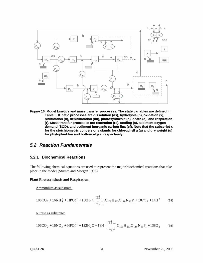
The sources and sinks for the state variables are depicted in Figure 16. The mathematical representation of these processes are presented in the following sections.
QUAL2K 31 November 25, 2003
rcn
rcp
rdx
cf
h
d
r
rpx
rnx
dnhna
s
smo
mi
hpi
cs
rnd
rpd
rcd
dsno
po sapab
sodcfcT o
s
Alksx
nnn
p
cT o
xcT o
Figure 16 Model kinetics and mass transfer processes. The state variables are defined in
Table 5. Kinetic processes are dissolution (ds), hydrolysis (h), oxidation (x), nitrification (n), denitrification (dn), photosynthesis (p), death (d), and respiration (r). Mass transfer processes are reaeration (re), settling (s), sediment oxygen demand (SOD), and sediment inorganic carbon flux (cf). Note that the subscript x for the stoichiometric conversions stands for chlorophyll a (a) and dry weight (d) for phytoplankton and bottom algae, respectively.
5.2 Reaction Fundamentals
5.2.1 Biochemical Reactions The following chemical equations are used to represent the major biochemical reactions that take place in the model (Stumm and Morgan 1996): Plant Photosynthesis and Respiration:
Ammonium as substrate:
+−+ ++←→
+++ H14O107PNOHCOH108HPONH16106CO 2116110263106R
P
22442 (58)
Nitrate as substrate:
2116110263106R
P+
22432 O138PNOHC18H+OH122HPONO16106CO +
←→
+++ −− (59)

QUAL2K 32 November 25, 2003
Nitrification:
+−+ ++→+ 2H OH NO 2O NH 2324 (60)
Denitrification:
O7H 2N 5CO 4H 4NO O5CH 22232 ++→++ +− (61)
Note that a number of additional reactions are used in the model such as those involved with
simulating pH and unionized ammonia. These will be outlined when these topics are discussed later in this document.
5.2.2 Stoichiometry of Organic Matter The model requires that the stoichiometry of organic matter (i.e., plants and detritus) be specified by the user. The following representation is suggested as a first approximation (Redfield et al. 1963, Chapra 1997),
mgA 1000 : mgP 1000 : mgN 7200 : gC 40 : gD 100 (62)
where gX = mass of element X [g] and mgY = mass of element Y [mg]. The terms D, C, N, P, and A refer to dry weight, carbon, nitrogen, phosphorus, and chlorophyll a, respectively. It should be noted that chlorophyll a is the most variable of these values with a range of approximately 500-2000 mgA (Laws and Chalup 1990, Chapra 1997).
These values are then combined to determine stoichiometric ratios as in
gYgX=xyr (63)
For example, the amount of nitrogen that is released when 1 gD of detritus is dissolved can be computed as
gDmgN72
gD 100mgN 7200 ==ndr
5.2.2.1 Oxygen Generation and Consumption The model requires that the rates of oxygen generation and consumption be prescribed. If ammonia is the substrate, the following ratio (based on Equation 62) can be used to determine the grams of oxygen generated for each gram of plant matter that is produced through photosynthesis.
gC gO
69.2)gC/moleC 12(moleC 106
)/moleOgO 32(moleO 107 2222 ==ocar (64)
If nitrate is the substrate, the following ratio (based on Equation 63) applies
QUAL2K 33 November 25, 2003
gC gO
47.3)gC/moleC 12(moleC 106
)/moleOgO 32(moleO 138 2222 ==ocnr (65)
Note that Equation (68) is also used for the stoichiometry of the amount of oxygen consumed for both plant respiration and fast organic CBOD oxidation.
For nitrification, the following ratio is based on Equation (64)
gNgO
57.4)gN/moleN 14(moleN 1
)/moleOgO 32(moleO 2 2222 ==onr (66)
5.2.2.2 CBOD Utilization Due to Denitrification As represented by Equation (60), CBOD is utilized during denitrification,
mgNgO
0.00286mgN 1000
gN 1gN/moleN 14 moleN 4gC/moleC 12moleC 5
gCgO
67.2 22 =×××=ondnr (67)
5.2.3 Temperature Effects on Reactions The temperature effect for all first-order reactions used in the model is represented by
20)20()( −= TkTk θ (68)
where k(T) = the reaction rate [/d] at temperature T [oC] and θ = the temperature coefficient for the reaction.
5.3 Constituent Reactions The mathematical relationships that describe the individual reactions and concentrations of the model state variables (Table 5) are presented in the following paragraphs.
5.3.1 Conservative Substance (s) By definition, conservative substances are not subject to reactions:
Ss = 0 (69)
5.3.2 Phytoplankton (ap) Phytoplankton increase due to photosynthesis. They are lost via respiration, death, and settling
PhytoSettl PhytoDeath PhytoResp PhytoPhoto −−−=apS (70)

QUAL2K 34 November 25, 2003
5.3.2.1 Photosynthesis Phytoplankton photosynthesis is a function of temperature, nutrients, and light
pp aµ PhytoPhoto = (71)
where µp = phytoplankton photosynthesis rate [/d], which is calculated as
LpNpgpp Tk φφµ )( = (72)
where kgp(T) = the maximum photosynthesis rate at temperature T [/d], φNp = phytoplankton nutrient attenuation factor [dimensionless number between 0 and 1], and φLp = the phytoplankton light attenuation coefficient [dimensionless number between 0 and 1]. Nutrient Limitation. Michaelis-Menten equations are used to represent growth limitation for inorganic nitrogen and phosphorus. The minimum value is then used to compute the nutrient attenuation factor,
++++
=isPp
i
nasNp
naNp pk
pnnk
nn,minφ (73)
where ksNp = nitrogen half-saturation constant [µgN/L] and ksPp = phosphorus half-saturation constant [µgP/L]. Light Limitation. It is assumed that light attenuation through the water follows the Beer-Lambert law,
zkeePARzPAR −= )0()( (74)
where PAR(z) = photosynthetically available radiation (PAR) at depth z below the water surface [ly/d]2, and ke = the light extinction coefficient [m−1]. The PAR at the water surface is assumed to be a fixed fraction of the solar radiation
)0( 47.0)0( IPAR = (75)
The extinction coefficient is related to model variables by
3/2
ppnppooiiebe aammkk αααα ++++= (76)
where keb = the background coefficient accounting for extinction due to water and color [/m], αi, αo, αp, and αpn, are constants accounting for the impacts of inorganic suspended solids [L/mgD/m], particulate organic matter [L/mgD/m], and chlorophyll [L/µgA/m and (L/µgA)2/3/m], respectively. Suggested values for these coefficients are listed in Table 6. 2 ly/d = langley per day. A langley is equal to a calorie per square centimeter. Note that a ly/d is related to the µE/m2/d by the following approximation: 1 µE/m2/s ≅ 0.45 Langley/day (LIC-OR, Lincoln, NE).
QUAL2K 35 November 25, 2003
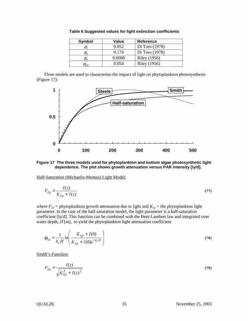
Table 6 Suggested values for light extinction coefficients
Symbol Value Reference αi 0.052 Di Toro (1978) αo 0.174 Di Toro (1978) αp 0.0088 Riley (1956) αpn 0.054 Riley (1956)
Three models are used to characterize the impact of light on phytoplankton photosynthesis
(Figure 17):
0
0.5
1
0 100 200 300 400 500
Steele
Half-saturation
Smith
Figure 17 The three models used for phytoplankton and bottom algae photosynthetic light
dependence. The plot shows growth attenuation versus PAR intensity [ly/d]. Half-Saturation (Michaelis-Menten) Light Model:
)()(
zIKzIF
LpLp +
= (77)
where FLp = phytoplankton growth attenuation due to light and KLp = the phytoplankton light parameter. In the case of the half-saturation model, the light parameter is a half-saturation coefficient [ly/d]. This function can be combined with the Beer-Lambert law and integrated over water depth, H [m], to yield the phytoplankton light attenuation coefficient
+
+=
− HkLp
Lp
eLp
eeIK
IKHk )0(
)0(ln1φ (78)
Smith’s Function:
22 )(
)(
zIK
zIFLp
Lp+
= (79)
QUAL2K 36 November 25, 2003
where KLp = the Smith parameter for phytoplankton [ly/d]; that is, the PAR at which growth is 70.7% of the maximum. This function can be combined with the Beer-Lambert law and integrated over water depth to yield
( )( ) ( )( )
++
++=
−− 2
2
/)0(1 /)0(
/)0(1/)0(ln1
HkLp
HkLp
LpLp
eLp
ee eKIeKI
KIKI
Hkφ (80)
Steele’s Equation:
LpKzI
LpLp e
KzIF
)( 1)( −= (81)
where KLp = the PAR at which phytoplankton growth is optimal [ly/d]. This function can be combined with the Beer-Lambert law and integrated over water depth to yield
−=−− −
Lp
Hek
Lp KIe
KI
eLp ee
Hk
)0( )0( 718282.2φ (82)
5.3.2.2 Losses
Respiration. Phytoplankton respiration is represented as a first-order rate that is attenuated at low oxygen concentration,
prp aTk )( PhytoResp = (83)
where krp(T) = temperature-dependent phytoplankton respiration rate [/d]. Death. Phytoplankton death is represented as a first-order rate,
pdp aTk )( PhytoDeath = (84)
where kdp(T) = temperature-dependent phytoplankton death rate [/d].
Settling. Phytoplankton settling is represented as
pa a
Hv
PhytoSettl = (85)
where va = phytoplankton settling velocity [m/d].
5.3.3 Bottom algae (ab) Bottom algae increase due to photosynthesis. They are lost via respiration and death.

QUAL2K 37 November 25, 2003
hBotAlgDeat BotAlgResp oBotAlgPhot −−=abS (86)
5.3.3.1 Photosynthesis
The representation of bottom algae photosynthesis is a simplification of a model developed by Rutherford et al. (1999). Photosynthesis is based on a temperature-corrected zero-order rate attenuated by nutrient and light limitation,
LbNbgb TC φφ)( oBotAlgPhot = (87)
where Cgb(T) = the temperature-dependent maximum photosynthesis rate [gD/(m2 d)], φNb = bottom algae nutrient attenuation factor [dimensionless number between 0 and 1], and φLb = the bottom algae light attenuation coefficient [dimensionless number between 0 and 1].
Temperature Effect. As for the first-order rates, an Arrhenius model is employed to quantify the effect of temperature on bottom algae photosynthesis,
20)20()( −= T
gbgb CTC θ (88)
Nutrient Limitation. Michaelis-Menten equations are used to represent growth limitation due to inorganic nitrogen and phosphorus. The minimum value is then used to compute the nutrient attenuation coefficient,
++++
=isPb
i
nasNb
naNb pk
pnnk
nn,minφ (89)
where ksNb = nitrogen half-saturation constant [µgN/L] and ksPb = phosphorus half-saturation constant [µgP/L]. Light Limitation. In contrast to the phytoplankton, light limitation at any time is determined by the amount of PAR reaching the bottom of the water column. This quantity is computed with the Beer-Lambert law (recall Equation 78) evaluated at the bottom of the river,
HkeeIHI −= )0()( (90)
As with the phytoplankton, three models (Equations 81, 83, and 85) are used to characterize
the impact of light on bottom algae photosynthesis. Substituting Equation (97) into these models yields the following formulas for the bottom algae light attenuation coefficient, Half-Saturation Light Model:
HkLb
Hk
Lb e
e
eIKeI
−
−
+=
)0()0(φ (91)
Smith’s Function:

QUAL2K 38 November 25, 2003
( )22 )0(
)0(Hk
Lb
Hk
Lpe
e
eIK
eI−
−
+=φ (92)
Steele’s Equation:
Lb
Hek
e KeI
Lb
Hk
Lb eKeI
−+−
=)0(1)0(φ (93)
where KLb = the appropriate bottom algae light parameter for each light model.
5.3.3.2 Losses
Respiration. Bottom algae respiration is represented as a first-order rate that is attenuated at low oxygen concentration,
brb aTk )( BotAlgResp = (94)
where krb(T) = temperature-dependent bottom algae respiration rate [/d].
Death. Bottom algae death is represented as a first-order rate,
bdb aTk )( h BotAlgDeat = (95)
where kdb(T) = the temperature-dependent bottom algae death rate [/d].
5.3.4 Detritus (mo) Detritus or particulate organic matter (POM) increases due to plant death. It is lost via dissolution and settling
DetrSettl DetrDiss hBotAlgDeat PhytoDeath −−+= damo rS (96)
where
odt mTk )( DetrDiss = (97)
where kdt(T) = the temperature-dependent detritus dissolution rate [/d] and
odt m
Hv
DetrSettl = (98)
where vdt = detritus settling velocity [m/d].

QUAL2K 39 November 25, 2003
5.3.5 Slowly Reacting CBOD (cs) Slowly reacting CBOD increases due to detritus dissolution. It is lost via hydrolysis.
SlowCHydr DetrDiss −= odcs rS (99)
where
shc cTk )( SlowCHydr = (100)
where khc(T) = the temperature-dependent slow CBOD hydrolysis rate [/d].
5.3.6 Fast Reacting CBOD (cf) Fast reacting CBOD is gained via the hydrolysis of slowly-reacting CBOD. It is lost via oxidation and denitrification.
Denitr OxidFastC SlowCHydr ondncf rS −−= (101)
where
fdcoxcf cTkF )( FastCOxid = (102)
where kdc(T) = the temperature-dependent fast CBOD oxidation rate [/d] and Foxcf = attenuation due to low oxygen [dimensionless]. The parameter rondn is the ratio of oxygen equivalents lost per nitrate nitrogen that is denitrified (Equation 71). The term Denitr is the rate of denitrification [µgN/L/d]. It will be defined in 5.3.10 below.
Three formulations are used to represent the oxygen attenuation: Half-Saturation:
oKoF
socfoxrp +
= (103)
where Ksocf = half-saturation constant for the effect of oxygen on fast CBOD oxidation [mgO2/L]. Exponential:
)1( oKoxrp
socfeF −−= (104)
where Ksocf = exponential coefficient for the effect of oxygen on fast CBOD oxidation [L/mgO2]. Second-Order Half Saturation:

QUAL2K 40 November 25, 2003
2
2
oKoF
socfoxrp
+= (105)
where Ksocf = half-saturation constant for second-order effect of oxygen on fast CBOD oxidation [mgO2
2/L2].
5.3.7 Dissolved Organic Nitrogen (no) Dissolved organic nitrogen increases due to detritus dissolution. It is lost via hydrolysis.
DONHydr DetrDiss −= ndno rS (106)
ohn nTk )( DONHydr = (107)
where khn(T) = the temperature-dependent organic nitrogen hydrolysis rate [/d].
5.3.8 Ammonia Nitrogen (na) Ammonia nitrogen increases due to dissolved organic nitrogen hydrolysis and plant respiration. It is lost via nitrification and plant photosynthesis:
oBotAlgPhot PhytoPhoto
NH4Nitrif BotAlgResp PhytoResp DONHydr
abndapna
ndnana
PrPr
rrS
−−
−++= (108)
The ammonia nitrification rate is computed as
anoxna nTkF )( NH4Nitrif = (109)
where kn(T) = the temperature-dependent nitrification rate for ammonia nitrogen [/d] and Foxna = attenuation due to low oxygen [dimensionless]. Oxygen attenuation is modeled by Equations (106) to (108) with the oxygen dependency represented by the parameter Ksona.
The coefficients Pap and Pap are the preferences for ammonium as a nitrogen source for
phytoplankton and bottom algae, respectively,
))(())(( nhnxpna
hnxpa
nhnxpahnxp
naap nknn
knnknk
nnP
+++
++= (110)
))(())(( nhnxbna
hnxba
nhnxbahnxb
naab nknn
knnknk
nnP
+++
++= (111)
where khnxp = preference coefficient of phytoplankton for ammonium [mgN/m3] and khnxb = preference coefficient of bottom algae for ammonium [mgN/m3].

QUAL2K 41 November 25, 2003
5.3.9 Unionized Ammonia The model simulates total ammonia. In water, the total ammonia consists of two forms: ammonium ion, NH4
+, and unionized ammonia, NH3. At normal pH (6 to 8), most of the total ammonia will be in the ionic form. However at high pH, unionized ammonia predominates. The amount of unionized ammonia can be computed as
auau nFn = (112)
where nau = the concentration of unionized ammonia [µgN/L], and Fu = the fraction of the total ammonia that is in unionized form,
au
KF pH101
1−+
= (113)
where Ka = the equilibrium coefficient for the ammonia dissociation reaction, which is related to temperature by
aa T
K 92.272909018.0p += (114)
where Ta is absolute temperature [K] and pKa = −log10(Ka).
5.3.10 Nitrate Nitrogen (nn) Nitrate nitrogen increases due to nitrification of ammonia. It is lost via denitrification and plant photosynthesis:
oBotAlgPhot )1(
PhytoPhoto )1(Denitr NH4Nitrif
abnd
apnani
Pr
PrS
−−
−−−= (115)
The denitrification rate is computed as
ndnoxdn nTkF )()(1 Denitr −= (116)
where kdn(T) = the temperature-dependent denitrification rate of nitrate nitrogen [/d] and Foxdn = effect of low oxygen on denitrification [dimensionless] as modeled by Equations (106) to (108) with the oxygen dependency represented by the parameter Ksodn.
5.3.11 Dissolved Organic Phosphorus (po) Dissolved organic phosphorus increases due to dissolution of detritus. It is lost via hydrolysis.
DOPHydr DetrDiss −= pdpo rS (117)

QUAL2K 42 November 25, 2003
where
ohp pTk )( DOPHydr = (118)
where khp(T) = the temperature-dependent organic phosphorus hydrolysis rate [/d].
5.3.12 Inorganic Phosphorus (pi) Inorganic phosphorus increases due to dissolved organic phosphorus hydrolysis and plant respiration. It is lost via plant photosynthesis:
oBotAlgPhotPhytoPhoto
BotAlgResp PhytoResp DOPHydr
pdpa
pdpapi
rr
rrS
−−
++= (119)
5.3.13 Inorganic Suspended Solids (mi) Inorganic suspended solids are lost via settling,
Smi = – InorgSettl where
ii m
Hv
InorgSettl= (120)
where vi = inorganic suspended solids settling velocity [m/d].
5.3.14 Dissolved Oxygen (o) Dissolved oxygen increases due to plant photosynthesis. It is lost via fast CBOD oxidation, nitrification and plant respiration. Depending on whether the water is undersaturated or oversaturated it is gained or lost via reaeration,
OxReaer BotAlgResp PhytoResp
NH4Nitr FastCOxidthBotAlgGrow hPhytoGrowt
+−−
−−+=
odoa
onocdooao
rr
rrrrS (121)
where
( )oelevToTk sa −= ),()(OxReaer (122)
where ka(T) = the temperature-dependent oxygen reaeration coefficient [/d], os(T, elev) = the saturation concentration of oxygen [mgO2/L] at temperature, T, and elevation above sea level, elev.

QUAL2K 43 November 25, 2003
5.3.14.1 Oxygen Saturation The following equation is used to represent the dependence of oxygen saturation on temperature (APHA 1992)
4
11
3
10
2
75
10621949.810243800.1
10642308.610575701.134411.139)0 ,(ln
aa
aas
TT
TTTo
×−×+
×−×+−=
(123)
where os(T, 0) = the saturation concentration of dissolved oxygen in freshwater at 1 atm [mgO2/L] and Ta = absolute temperature [K] where Ta = T +273.15.
The effect of elevation is accounted for by
)0001148.01(),( )0 ,(ln eleveelevTo Tos
s −= (124)
where elev = the elevation above sea level [m].
5.3.14.2 Reaeration Formulas The reaeration coefficient can be prescribed on the Reach worksheet. If reaeration is not prescribed, it can be computed using one of the following formulas: O’Connor-Dobbins:
5.1
5.093.3)20(
HUka = (125)
Owens-Gibbs:
85.1
67.032.5)20(
HUka = (126)
Churchill:
67.1026.5)20(H
Uka = (127)
where U = velocity [m/s] and H = depth [m].
Reaeration can also be internally calculated based on the following scheme patterned after a
plot developed by Covar (1976) (Figure 18): � If H < 0.61 m, use the Owens-Gibbs formula

QUAL2K 44 November 25, 2003
� If H > 0.61 m and H > 3.45U2.5, use the O’Connor-Dobbins formula � Otherwise, use the Churchill formula
This is referred to as option Internal on the Rates worksheet of Q2K.
0.1
1
10
Dep
th (m
)
0.1 1Velocity (mps)
OwensGibbs
10
100
O’ConnorDobbins
0.1
1
0.2
0.5
Chu
rchi
ll
0.05
2
2050
5
Figure 18 Reaeration rate (/d) versus depth and velocity (Covar 1976).
5.3.14.3 Effect of Control Structures: Oxygen Oxygen transfer in streams is influenced by the presence of control structures such as weirs, dams, locks, and waterfalls (Figure 19). Butts and Evans (1983) have reviewed efforts to characterize this transfer and have suggested the following formula,
)046.01)(11.01(38.01 THHbar ddddd +−+= (128)
where rd = the ratio of the deficit above and below the dam, Hd = the difference in water elevation [m] as calculated with Equation (7), T = water temperature (°C) and ad and bd are coefficients that correct for water-quality and dam-type. Values of these coefficients are summarized in Table 7.
Qi−−−−1 o’i−−−−1Hd
Qi−−−−1 oi−−−−1
i −−−− 1 i

QUAL2K 45 November 25, 2003
Figure 19 Water flowing over a river control structure.
Table 7 Coefficient values used to predict the effect of dams on stream reaeration.
(a) Water-quality coefficient Polluted state ad Gross 0.65 Moderate 1.0 Slight 1.6 Clean 1.8 (b) Dam-type coefficient Dam type bd Flat broad-crested regular step 0.70 Flat broad-crested irregular step 0.80 Flat broad-crested vertical face 0.60 Flat broad-crested straight-slope face 0.75 Flat broad-crested curved face 0.45 Round broad-crested curved face 0.75 Sharp-crested straight-slope face 1.00 Sharp-crested vertical face 0.80 Sluice gates 0.05
The oxygen mass balance for the reach below the structure is written as
( ) ioi
ioii
i
ii
i
iabi
i
ii
i
ii SV
Woo
VE
oV
Qo
VQ
oV
Qdt
do,
,1
',
11 ' ++−+−−= +−− (129)
where o’i−1 = the oxygen concentration entering the reach [mgO2/L], where
d
iisisi r
oooo 11,
1,1' −−−−
−−= (130)
5.3.15 Pathogen (x) Pathogens are subject to death and settling,
PathSettlPathDeath −−=xS (131)
5.3.15.1 Death Pathogen death is due to natural die-off and light (Chapra 1997). The death of pathogens in the absence of light is modeled as a first-order temperature-dependent decay and the death rate due to light is based on the Beer-Lambert law,
QUAL2K 46 November 25, 2003
( )xeHk
IxTk Hk
edx
e−−+= 124/)0()( PathDeath (132)
where kdx(T) = temperature-dependent pathogen die-off rate [/d].
5.3.15.2 Settling Pathogen settling is represented as
xHvx PathSettl = (133)
where vx = pathogen settling velocity [m/d].
5.3.16 pH The following equilibrium, mass balance and electroneutrality equations define a freshwater dominated by inorganic carbon (Stumm and Morgan 1996),
]COH[]H][HCO[
*32
31
+−=K (134)
]HCO[]H][CO[
3
23
2 −
+−=K (135)
]OH][H[ −+=wK (136)
]CO[]HCO[]COH[ 2
33*32
−− ++=Tc (137)
][H]OH[]CO[2]HCO[ 2
33+−−− −++=Alk (138)
where K1, K2 and Kw are acidity constants, Alk = alkalinity [eq L−1], H2CO3* = the sum of dissolved carbon dioxide and carbonic acid, HCO3
− = bicarbonate ion, CO32− = carbonate ion, H+
= hydronium ion, OH− = hydroxyl ion, and cT = total inorganic carbon concentration [mole L−1]. The brackets [ ] designate molar concentrations.
Note that the alkalinity is expressed in units of eq/L for the internal calculations. For input and output, it is expressed as mgCaCO3/L. The two units are related by
eq/L)(000,50)/LmgCaCO( 3 AlkAlk ×= (139)
The equilibrium constants are corrected for temperature by
Harned and Hamer (1933):
QUAL2K 47 November 25, 2003
80.22010365.0)(log 1321.73.4787=p 10 −++ aaa
w TTT
K (140)
Plummer and Busenberg (1982):
21
/915,684,1log8339.126 /37.2183406091964.0356.3094=log
aa
aaTT
TTK−+
+−− (141)
Plummer and Busenberg (1982):
22
/9.713,563log92561.38 /79.515103252849.08871.107=log
aa
aaTT
TTK−+
+−− (142)
The nonlinear system of five simultaneous equations (138 through 142) can be solved
numerically for the five unknowns: [H2CO3*], [HCO3−], [CO3
2−], [OH−], and {H+}. As presented Stumm and Morgan (1996), an efficient solution method can be derived by combining Equations (138), (139) and (141) to define the quantities (Stumm and Morgan 1996)
2112
2
0+][H][H
][HKKK ++
+
+=α (143)
2112
11
+][H][H][H
KKKK
++
+
+=α (144)
2112
212
+][H][H KKKKK
++ +=α (145)
where α0, α1, and α2 = the fraction of total inorganic carbon in carbon dioxide, bicarbonate, and carbonate, respectively. Equations (140), (142), (148) and (149) can then be combined to yield,
]H[][H
)2(=Alk 21+
+−++ w
TK
cαα (146)
Thus, solving for pH reduces to determining the root, {H+}, of
Alk]H[][H
)2(=])H([ 21 −−++ ++
+ wT
Kcf αα (147)
where pH is then calculated with
]H[logpH 10+−= (148)
The root of Equation (151) is determined with the bisection method (Chapra and Canale 2002).
5.3.17 Total Inorganic Carbon (cT)
QUAL2K 48 November 25, 2003
Total inorganic carbon concentration increases due to fast carbon oxidation and plant respiration. It is lost via plant photosynthesis. Depending on whether the water is undersaturated or oversaturated with CO2, it is gained or lost via reaeration,
CO2Reaer oBotAlgPhotPhytoPhoto
BotAlgResp PhytoRespFastCOxid
+−−
++=
ccdcca
ccdccaccccT
rr
rrrS (149)
where
( )Tsac cTk 02 ][CO)(CO2Reaer α−= (150)
where kac(T) = the temperature-dependent carbon dioxide reaeration coefficient [/d], and [CO2]s = the saturation concentration of carbon dioxide [mole/L].
The stoichiometric coefficients are derived from Equation (62)3
L 1000m
gC 12moleC
mgAgC 3
××
= cacca rr (151)
L 1000m
gC 12moleC
gDgC 3
××
= cdccd rr (152)
L 1000m
gC 12moleC 3
×=cccr (153)
5.3.17.1 Carbon Dioxide Saturation The CO2 saturation is computed with Henry’s law,
2COs2 p][CO HK= (154)
where KH = Henry's constant [mole (L atm)−1] and pCO2 = the partial pressure of carbon dioxide in the atmosphere [atm]. Note that users input the partial pressure to Q2K in ppm. The program internally converts ppm to atm using the conversion: 10−6 atm/ppm.
The value of KH can be computed as a function of temperature by (Edmond and Gieskes 1970)
0184.140.01526422385.73=p H +−− aa
TT
K (155)
3 The conversion, m3 = 1000 L is included because all mass balances express volume in m3, whereas total
inorganic carbon is expressed as mole/L.

QUAL2K 49 November 25, 2003
The partial pressure of CO2 in the atmosphere has been increasing, largely due to the combustion of fossil fuels (Figure 20). Values in 2003 are approximately 10-3.43 atm (= 372 ppm).
Figure 20 Concentration of carbon dioxide in the atmosphere as recorded at Mauna Loa Observatory, Hawaii. (http://www.cmdl.noaa.gov/ccg/figures/co2mm_mlo.jpg).
5.3.17.2 CO2 Gas Transfer The CO2 reaeration coefficient can be computed from the oxygen reaeration rate by
)20( 923.0)20(4432)20(
25.0
aaac kkk =
= (156)
5.3.17.3 Effect of Control Structures: CO2 As was the case for dissolved oxygen, carbon dioxide gas transfer in streams can be influenced by the presence of control structures. Q2K assumes that carbon dioxide behaves similarly to dissolved oxygen (recall Sec. 5.3.14.3). Thus, the inorganic carbon mass balance for the reach immediately downstream of the structure is written as
( ) icTi
icTiTiT
i
iiT
i
iabiT
i
iiT
i
iiT SV
Wcc
VE
cV
Qc
VQ
cV
Qdt
dc,
,,1,
'
,,
,1,1, ' ++−+−−= +−− (157)
where c'T,i−1 = the concentration of inorganic carbon entering the reach [mgO2/L], where

QUAL2K 50 November 25, 2003
d
iTisisiTiT r
cCOCOcc 1,21,,2
1,,21,211, )(' −−−−−
−−++=
ααα (158)
where rd is calculated with Equation (132).
5.3.18 Alkalinity (Alk) The present model accounts for changes in alkalinity due to plant photosynthesis and respiration, nitrification, and denitrification.
( )( )
Denitr NH4Nitr
BotAlgResp th BotAlgGrow )1(
PhytoResp PhytoPhoto )1(
alkdenalkn
alkdaapalkdnapalkda
alkaaapalkanapalkaaalk
rr
rPrPr
rPrPrS
+−
+−+−+
+−+−=
(159)
where the r’s are ratios that translate the processes into the corresponding amount of alkalinity. The stoichiometric coefficients are derived from Equations (62) through (65) as in
Phytoplankton Photosynthesis (Ammonia as Substrate) and Respiration:
L 1000m
gC 12moleC
moleC 106eqH 14
mgAgC 3
×××
=
+
caalkaa rr (160)
Phytoplankton Photosynthesis (Nitrate as Substrate):
L 1000m
gC 12moleC
moleC 106eqH 81
mgAgC 3
×××
=
+
caalkan rr (161)
Bottom Algae Photosynthesis (Ammonia as Substrate) and Respiration:
L 1000m
gC 12moleC
moleC 106eqH 14
gDgC 3
×××
=
+
caalkda rr (162)
Bottom Algae Photosynthesis (Nitrate as Substrate):
L 1000m
gC 12moleC
moleC 106eqH 81
gDgC 3
×××
=
+
caalkdn rr (163)
Nitrification:
L 1000m 1
mgN 1000gN 1
gN 14moleN
moleN 1eqH 2 3
×××=+
alknr (164)
Denitrification:

QUAL2K 51 November 25, 2003
L 1000m 1
mgN 1000gN 1
gN 14moleN
moleN 1eqH 4 3
×××=+
alkdenr (165)
5.4 SOD/Nutrient Flux Model Sediment nutrient fluxes and sediment oxygen demand (SOD) are based on a model developed by Di Toro (Di Toro et al. 1991, Di Toro and Fitzpatrick. 1993, Di Toro 2001). The present version also benefited from James Martin’s (Mississippi State University, personal communication) efforts to incorporate the Di Toro approach into EPA’s WASP modeling framework.
A schematic of the model is depicted in Figure 21. As can be seen, the approach allows oxygen and nutrient sediment-water fluxes to be computed based on the downward flux of particulate organic matter from the overlying water. The sediments are divided into 2 layers: a thin (≅ 1 mm) surface aerobic layer underlain by a thicker (10 cm) lower anaerobic layer. Organic carbon, nitrogen and phosphorus are delivered to the anaerobic sediments via the settling of particulate organic matter (i.e., phytoplankton and detritus). There they are transformed by mineralization reactions into dissolved methane, ammonium and inorganic phosphorus. These constituents are then transported to the aerobic layer where some of the methane and ammonium are oxidized. The flux of oxygen from the water required for these oxidations is the sediment oxygen demand. The following sections provide details on how the model computes this SOD along with the sediment-water fluxes of carbon, nitrogen and phosphorus that are also generated in the process.
CH4 NO3
NO3
NH4d PO4p PO4d
NH4p NH4d
PO4p PO4d
CO2 N2
N2
POC
cf o na nn pioJpom
NH4p
CH4(gas)
POP
DIAGENESIS METHANE AMMONIUM NITRATE PHOSPHATE
AER
OB
ICA
NA
ERO
BIC
WA
TER
PON
Figure 21 Schematic of SOD-nutrient flux model of the sediments.
QUAL2K 52 November 25, 2003
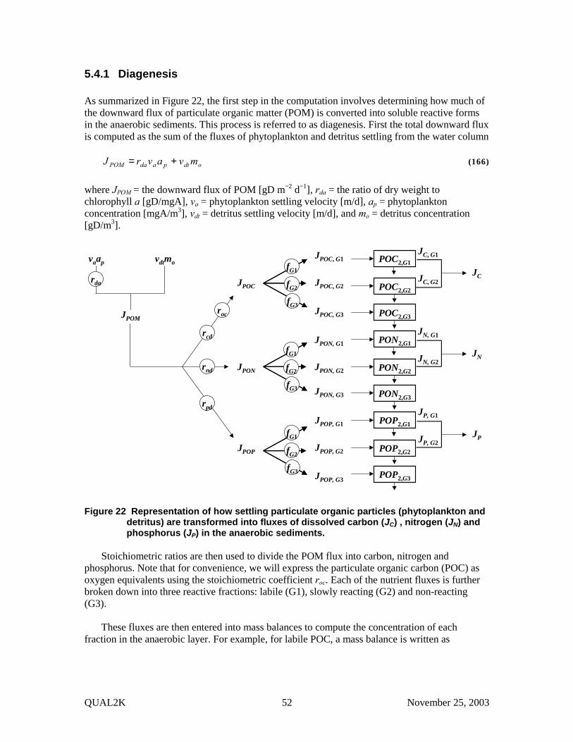
5.4.1 Diagenesis As summarized in Figure 22, the first step in the computation involves determining how much of the downward flux of particulate organic matter (POM) is converted into soluble reactive forms in the anaerobic sediments. This process is referred to as diagenesis. First the total downward flux is computed as the sum of the fluxes of phytoplankton and detritus settling from the water column
odtpadaPOM mvavrJ += (166)
where JPOM = the downward flux of POM [gD m−2 d−1], rda = the ratio of dry weight to chlorophyll a [gD/mgA], va = phytoplankton settling velocity [m/d], ap = phytoplankton concentration [mgA/m3], vdt = detritus settling velocity [m/d], and mo = detritus concentration [gD/m3].
JPOC, G1
JPOC, G2
JPOC, G3
JPON, G1
JPON, G2
JPON, G3
JPOP, G1
JPOP, G2
JPOP, G3
JPOC
JPON
JPOP
rcd
rnd
rpd
JCfG1
fG2
fG3
fG1
fG2
fG3
fG1
fG2
fG3
JPOM
rda
vaap vdtmo POC2,G1
POC2,G2
POC2,G3
JN
PON2,G1
PON2,G2
PON2,G3
JP
POP2,G1
POP2,G2
POP2,G3
roc
JC, G1
JC, G2
JN, G1
JN, G2
JP, G1
JP, G2
Figure 22 Representation of how settling particulate organic particles (phytoplankton and detritus) are transformed into fluxes of dissolved carbon (JC) , nitrogen (JN) and phosphorus (JP) in the anaerobic sediments.
Stoichiometric ratios are then used to divide the POM flux into carbon, nitrogen and
phosphorus. Note that for convenience, we will express the particulate organic carbon (POC) as oxygen equivalents using the stoichiometric coefficient roc. Each of the nutrient fluxes is further broken down into three reactive fractions: labile (G1), slowly reacting (G2) and non-reacting (G3).
These fluxes are then entered into mass balances to compute the concentration of each
fraction in the anaerobic layer. For example, for labile POC, a mass balance is written as

QUAL2K 53 November 25, 2003
1,221,2220
1,1,1,1,2
2 GGT
GPOCGPOCGPOCG POCwPOCHkJ
dtdPOC
H −−= −θ (167)
where H2 = the thickness of the anaerobic layer [m], POC2,G1 = the concentration of the labile fraction of POC in the anaerobic layer [gO2/m3], JPOC,G1 = the flux of labile POC delivered to the anaerobic layer [gO2/m2/d], kPOC,G1 = the mineralization rate of labile POC [d−1], θPOC,G1 = temperature correction factor for labile POC mineralization [dimensionless], and w2 = the burial velocity [m/d]. At steady state, Eq. 166 can be solved for
bT
GPOCGPOC
GPOCG vHk
JPOC
+= −
220
1,1,
1,1,2 θ
(168)
The flux of labile dissolved carbon, JC,G1 [gO2/m2/d], can then be computed as
1,2220
1,1,1, GT
GPOCGPOCGC POCHkJ −= θ (169)
In a similar fashion, a mass balance can be written and solved for the slowly reacting
dissolved organic carbon. This result is then added to Eq. 168 to arrive at the total flux of dissolved carbon generated in the anaerobic sediments.
2,1, GCGCC JJJ += (170)
Similar equations are developed to compute the diagenesis fluxes of nitrogen, JN [gN/m2/d], and phosphorus JP [gP/m2/d].
5.4.2 Ammonium Based on the mechanisms depicted in Figure 21, mass balances can be written for total ammonium in the aerobic layer and the anaerobic layers,
( ) ( )
1,412,41,44
4204
21,4
1,41
1,421,412,42121,412,42121,4
1
21000 NHf
oKo
NHKK
sNHf
ns
NHwNHfNHfKNHfNHfdt
dNHH
daONHNH
NHTNH
NHda
a
dadaLpapa
++−
−+
−−+−=
−θκ
ω (171)
( ) ( )
( )2,41,42
2,421,41122,421,41122,4
2
NHNHw
NHfNHfKNHfNHfJdt
dNHH dadaLpapaN
−+
−+−+= ω (172)
where H1 = the thickness of the aerobic layer [m], NH4,1 and NH4,2 = the concentration of total ammonium in the aerobic layer and the anaerobic layers, respectively [gN/m3], na = the ammonium concentration in the overlying water [mgN/m3], κNH4,1 = the reaction velocity for nitrification in the aerobic sediments [m/d], θNH4 = temperature correction factor for nitrification [dimensionless], KNH4 = ammonium half-saturation constant [gN/m3], o = the dissolved oxygen

QUAL2K 54 November 25, 2003
concentration in the overlying water [gO2/m3], and KNH4,O2 = oxygen half-saturation constant [mgO2/L], and JN = the diagenesis flux of ammonium [gN/m2/d].
The fraction of ammonium in dissolved (fdai) and particulate (fpai) form are computed as
aiidai m
fπ+
=1
1 (173)
daipai ff −=1 (174)
where mi = the solids concentration in layer i [gD/m3], and πai = the partition coefficient for ammonium in layer i [m3/gD].
The mass transfer coefficient for particle mixing due to bioturbation between the layers, ω12 [m/d], is computed as
oKo
POCrPOC
HD
DpMR
ocGTDpp
+=
−
,
1,2
2
20
12/θ
ω (175)
where Dp = diffusion coefficient for bioturbation [m2/d], θDp = temperature coefficient [dimensionless], POCR = reference G1 concentration for bioturbation [gC/m3] and KM,Dp = oxygen half-saturation constant for bioturbation [gO2/m3].
The mass transfer coefficient for pore water diffusion between the layers, KL12 [m/d], is computed as,
2/2
20
12 HD
KTDdd
L
−
=θ
(176)
where Dd = pore water diffusion coefficient [m2/d], and θDd = temperature coefficient [dimensionless].
The mass transfer coefficient between the water and the aerobic sediments, s [m/d], is computed as
oSODs = (177)
where SOD = the sediment oxygen demand [gO2/m2/d].
At steady state, Eqs. 170 and 171 are two simultaneous nonlinear algebraic equations. The
equations can be linearized by assuming that the NH4,1 term in the Monod term for nitrification is constant. The simultaneous linear equations can then be solved for NH4,1 and NH4,2. The flux of ammonium to the overlying water can then be computed as
−=10001,414
adaNH
nNHfsJ (178)

QUAL2K 55 November 25, 2003
5.4.3 Nitrate Mass balances for nitrate can be written for the aerobic and anaerobic layers as
( )
1,3203
21,3
1,412,41,44
4204
21,4
1,31,321,32,3121,3
1
2
1000
NOs
NHfoK
oNHK
Ks
NOn
sNOwNONOKdt
dNOH
TNO
NOda
ONHNH
NHTNH
NH
nL
−− −++
+
−+−−=
θκ
θκ (179)
( ) ( ) 2,32032,32,31,322,31,312
2,32 NONONOwNONOKJ
dtdNO
H TNONOLN−−−+−+= θκ (180)
where NO3,1 and NO3,2 = the concentration of nitrate in the aerobic layer and the anaerobic layers, respectively [gN/m3], nn = the nitrate concentration in the overlying water [mgN/m3], κNO3,1 and κNO3,2 = the reaction velocities for denitrification in the aerobic and anaerobic sediments, respectively [m/d], and θNO3 = temperature correction factor for denitrification [dimensionless].
In the same fashion as for Eqs. 170 and 171, Eqs. 178 and 179 can be linearized and solved for NO3,1 and NO3,2. The flux of nitrate to the overlying water can then be computed as
−=10001,33
nNO
nNOsJ (181)
Denitrification requires a carbon source as represented by the following chemical equation,
O7H 2N 5CO 4H 4NO O5CH 22232 ++→++ +− (182)
The carbon requirement (expressed in oxygen equivalents per nitrogen) can therefore be computed as
mgNgO
0.00286mgN 1000
gN 1gN/moleN 14 moleN 4gC/moleC 12moleC 5
gCgO
67.2 22 =×××=ondnr (183)
Therefore, the oxygen equivalents consumed during denitrification, JO2,dn [gO2/m2/d], can be computed as
+×= −−
2,32032,31,3
203
21,3
,2 gNmgN1000 NONO
srJ T
NONOTNO
NOondndnO θκθ
κ (184)
5.4.4 Methane The dissolved carbon generated by diagenesis is converted to methane in the anaerobic sediments. Because methane is relatively insoluble, its saturation can be exceeded and methane gas produced. As a consequence, rather than write a mass balance for methane in the anaerobic layer,

QUAL2K 56 November 25, 2003
an analytical model developed by Di Toro et al. (1990) is used to determine the steady-state flux of dissolved methane corrected for gas loss delivered to the aerobic sediments.
First, the carbon diagenesis flux is corrected for the oxygen equivalents consumed during denitrification,
dnOCTCH JJJ ,2,4 −= (185)
where JCH4,T = the carbon diagenesis flux corrected for denitrification [gO2/m2/d]. In other words, this is the total anaerobic methane production flux expressed in oxygen equivalents.
If JCH4,T is sufficiently large (≥ 2KL12Cs), methane gas will form. In such cases, the flux can be corrected for the gas loss,
TCHsLdCH JCKJ ,412,4 2= (186)
where JCH4,d = the flux of dissolved methane (expressed in oxygen equivalents) that is generated in the anaerobic sediments and delivered to the aerobic sediments [gO2/m2/d], Cs = the saturation concentration of methane expressed in oxygen equivalents [mgO2/L]. If JCH4,T < 2KL12Cs, then no gas forms and
TCHdCH JJ ,4,4 = (187)
The methane saturation concentration is computed as
T
sHC −
+= 20024.110
1100 (188)
where H = water depth [m] and T = water temperature [oC].
A methane mass balance can then be written for the aerobic layer as
( ) 1,4204
21,4
1,4,41,4
1 CHs
CHcsJdt
dCHH T
CHCH
fdCH−−−+= θ
κ (189)
where CH4,1 = methane concentration in the aerobic layer [gO2/m3], cf = fast CBOD in the overlying water [gO2/m3], κCH4,1 = the reaction velocity for methane oxidation in the aerobic sediments [m/d], and θCH4 = temperature correction factor [dimensionless]. At steady, state, this balance can be solved for
204
21,4
,41,4
−+
+=
TCH
CH
fdCH
ss
scJCH
θκ
(190)
The flux of methane to the overlying water, JCH4 [gO2/m2/d], can then be computed as
( )fCH cCHsJ −= 1,44 (191)

QUAL2K 57 November 25, 2003
5.4.5 SOD The SOD [gO2/m2/d] is equal to the sum of the oxygen consumed in methane oxidation and nitrification,
NSODCSODSOD += (192) where CSOD = the amount of oxygen demand generated by methane oxidation [gO2/m2/d] and NSOD = the amount of oxygen demand generated by nitrification [gO2/m2/d]. These are computed as
1,4204
21,4 CH
sCSOD T
CHCH −= θ
κ (193)
1,412,41,44
4204
21,4
2NHf
oKo
NHKK
srNSOD da
ONHNH
NHTNH
NHon ++
= −θκ
(194)
where ron = the ratio of oxygen to nitrogen consumed during nitrification [= 4.57 gO2/gN].
5.4.6 Inorganic Phosphorus Mass balances can be written total inorganic phosphorus in the aerobic layer and the anaerobic layers as
( ) ( )
−+−
−+−=
1,411,42
1,412,42121,412,42121,4
1
1000 POf
psPOw
POfPOfKPOfPOfdt
dPOH
dai
dpdpLppppω (195)
( ) ( )( )2,41,42
2,421,41122,421,41122,4
2
POPOw
POfPOfKPOfPOfJdt
dPOH dpdpLppppP
−+
−+−+= ω (196)
where PO4,1 and PO4,2 = the concentration of total inorganic phosphorus in the aerobic layer and the anaerobic layers, respectively [gP/m3], pi = the inorganic phosphorus in the overlying water [mgP/m3], and JP = the diagenesis flux of phosphorus [gP/m2/d].
The fraction of phosphorus in dissolved (fdpi) and particulate (fppi) form are computed as
piidpi m
fπ+
=1
1 (197)
dpippi ff −=1 (198)

QUAL2K 58 November 25, 2003
where πpi = the partition coefficient for inorganic phosphorus in layer i [m3/gD].
The partition coefficient in the anaerobic layer is set to an input value. For the aerobic layer, if the oxygen concentration in the overlying water column exceeds a critical concentration, ocrit [gO2/m3], then the partition coefficient is increased to represent the sorption of phosphorus onto iron oxyhydroxides as in
( )1,421 POpp πππ ∆= (199)
where ∆πPO4,1 is a factor that increases the aerobic layer partition coefficient relative to the anaerobic coefficient.
If the oxygen concentration falls below ocrit then the partition coefficient is decreased
smoothly until it reaches the anaerobic value at zero oxygen,
( ) critooPOpp
/1,421 πππ ∆= (200)
Equations 194 and 195 can be solved for PO4,1 and PO4,2. The flux of phosphorus to the
overlying water can then be computed as
−=10001,44
iPO
pPOsJ (201)
5.4.7 Solution Scheme Although the foregoing sequence of equations can be solved, a single computation will not yield a correct result because of the interdependence of the equations. For example, the surface mass transfer coefficient s depends on SOD. The SOD in turn depends on the ammonium and methane concentrations which themselves are computed via mass balances that depend on s. Hence, an iterative technique must be used. The procedure used in QUAL2K is
1. Determine the diagenesis fluxes: JC, JN and JP.
2. Start with an initial estimate of SOD,
NonCinit JrJSOD '+= (202)
where ron’ = the ratio of oxygen to nitrogen consumed for total conversion of ammonium to nitrogen gas via nitrification/denitrification [= 1.714 gO2/gN]. This ratio accounts for the carbon utilized for denitrification.
3. Compute s using
oSOD
s init= (203)
4. Solve for ammonium, nitrate and methane, and compute the CSOD and NSOD.

QUAL2K 59 November 25, 2003
5. Make a revised estimate of SOD using the following weighted average
2NSODCSODSOD
SOD init ++= (204)
6. Check convergence by calculating an approximate relative error
%100×−
=SOD
SODSOD initaε (205)
7. If εa is greater than a prespecified stopping criterion εs then set SODinit = SOD and return
to step 2.
8. If convergence is adequate (εa ≤ εs), then compute the inorganic phosphorus concentrations.
9. Compute the ammonium, nitrate, methane and phosphate fluxes.
5.4.8 Supplementary Fluxes
Because of the presence of organic matter deposited prior to the summer steady-state period (e.g., during spring runoff), it is possible that the downward flux of particulate organic matter is insufficient to generate the observed SOD. In such cases, a supplementary SOD can be prescribed,
st SODSODSOD += (206)
where SODt = the total sediment oxygen demand [gO2/m2/d], and SODs = the supplementary SOD [gO2/m2/d]. In addition, prescribed ammonia and methane fluxes can be used to supplement the computed fluxes.


QUAL2K 61 November 25, 2003
6 USERS MANUAL
6.1 OVERVIEW The computer code used to implement the calculations for QUAL2K is written in Visual Basic for Applications (VBA). Excel serves as the user interface. Color is used to signify whether information is to be input by the user or output by the program:
• Pale Blue designates variable and parameter values that are to be entered by the user. • Pale Yellow designates data that the user enters. This data are then displayed on graphs
generated by Q2K. • Pale Green designates output values generated by Q2K. • Dark solid colors are used for labels and should not be changed.
All worksheets include two buttons (Figure 23):
• Open Old Files. When this button is clicked, the file browser will automatically open to
allow you to access a data file. All QUAL2K data files have the extension, *.q2k. • Run. This button causes Q2K to execute and to create a data file that holds the input
values. The data file can then be accessed later using the Open Old File button.
Figure 23. The buttons used in Q2K.

QUAL2K 62 November 25, 2003
6.2 WORKSHEETS
6.2.1 QUAL2K Worksheet The QUAL2K Worksheet (Figure 24) is used to enter general information regarding a particular model application.
Figure 24. The QUAL2K Worksheet. River name. Name of the river or stream being modeled. After the program is run, this name along with the date, is displayed on all sheets and charts. File name. This is the name of the data file generated when Q2K is run. Directory where file saved. This specifies the complete path to the directory where the file is saved. Month. The simulation month. This is entered in numerical format (e.g., January = 1, February = 2, etc.). Day. The simulation day. Year. The simulation year (e.g., 1993) Time zone. A pull-down menu (Figure 25) allows you to select the proper U.S. time zone.

QUAL2K 63 November 25, 2003
Figure 25. The pull down menu for setting the time zone. Daylight savings time. A pull down menu allows you to specify whether daylight savings time is in effect (Yes or No). Calculation step. This is the time step used for the calculation. It must be less than or equal to 4 hrs. If the user enters a value greater than 4 hours, the program automatically sets the calculation step to 4 hours. This level of resolution is required in order to have a sufficient number of points to create smooth diel plots. Final time. This defines the duration of the calculation. It must be an integer that is greater than or equal to 2 days. This constraint is imposed because the model is run in a time variable mode until it reaches a steady state. Therefore, the first day of simulation is by definition overwhelmingly dominated by its initial conditions. If the user enters a value less than 2 days, the program automatically sets the final time to 2 days. The final time should be at least twice the river’s travel time. For streams with short travel times where bottom algae are simulated, it must usually be longer. Program determined calc step (output). The program takes the Calculation step entered by the user and then rounds it down to the next lowest whole base-2 number. In order to use a lower time step, you must reduce the calculation step below this value. Time of last calculation (output). The computer automatically displays the computer time required for the simulation. Time of sunrise. This is the time of sunrise for the farthest downstream reach. Time of solar noon. This is the time of solar noon for the farthest downstream reach. Time of sunset. This is the time of sunset for the farthest downstream reach. Photoperiod. This is the fraction of the day that the sun is up for the farthest downstream reach. It is equal to the time in hours between sunrise and sunset divided by 24.

QUAL2K 64 November 25, 2003
6.2.2 Headwater Worksheet This worksheet (Figure 26) is used to enter flow and concentration for the system’s boundaries.
Figure 26. The upper part of the Headwater Worksheet used to enter the headwater’s constant characteristics and to specify its hydraulics.
Flow. The headwater’s flow rate in m3/s. Prescribed Downstream Boundary? If the downstream boundary has an effect on the simulation, this option is set to yes. Headwater Water Quality. This block of cells is used to enter the temperature and water quality boundary conditions at the river’s headwater. For cases where the data varies in a diel fashion, Q2K allows you to enter values on an hourly basis. If the values are constant over the daily cycle, just enter the mean value for all times. Downstream Boundary Water Quality. If the downstream boundary has an effect on the simulation, this block of cells is used to enter the temperature and water quality conditions at the river’s downstream boundary. headwater.

QUAL2K 65 November 25, 2003
6.2.3 Reach Worksheet This worksheet is used to enter information related to the river’s headwater (Reach Number 0) and reaches (Figure 27 through Figure 31).
Figure 27. The first part of the Reach Worksheet used to specify reach labels, distances and elevations.
Reach for diel plot. Cell B6 is used to enter the number of the reach for which diel plots will be generated. If a negative, zero or a value greater than the number of reaches is entered, the program automatically sets the value to the last downstream reach. Reach Label (optional). Q2K allows you to enter identification labels for each reach. Figure 28 provides an example to illustrate the naming scheme. The first two reaches of a river are shown. Because it includes the Jefferson City WWTP discharge, we might choose to enter the reach label “Jefferson City WWTP” for the first reach. Similarly we might label the second reach as “Sampling Station 27.”
Route 11Bridge
Jefferson CityWWTP
Upstream endof reach 1 Downstream end
of reach 2
JeffersonDam
Downstream endof reach 1
Headwater
SamplingStation 27
Figure 28. The first two reaches of a river system. Downstream end of reach label (optional). Q2K allows you to enter identification labels for the boundaries between reaches. These labels are then displayed on other worksheets to identify the reaches. As shown in Figure 29, the downstream end of the first reach in Figure 28 could be labeled as “Jefferson Dam”. Similarly, the downstream end of the second reach could be labeled as “Route 11 Bridge”.

QUAL2K 66 November 25, 2003
Figure 29. An example of the labels that could be entered for the reaches in Figure 28.
Reach numbers (output). The model automatically numbers the reaches in ascending order. Reach length (output). The model automatically computes and displays the length of each reach. Downstream Latitude and Longitude (output). The model automatically computes and displays the latitude and longitude of the downstream ends of each reach in decimal degrees. Downstream location. The user must enter the river kilometer for the downstream end of each reach. Note that the reach distances can be in descending or ascending order. Upstream and downstream elevation. The user must enter the elevation in meters above sea level for both the upstream and downstream ends of the reach. Downstream Latitude and Longitude (output). The user must enter the latitude and longitude of the downstream end of each reach in degrees, minutes, and seconds. Alternatively, they can be entered in decimal degrees, in which case, the minutes and seconds entries would be left blank or zero.
Figure 30. The part of the Reach Worksheet used to specify the system’s hydraulics. Hydraulic Model. Q2K allows two options for computing velocity and depth based on flow: (1) rating curves or (2) the Manning formula. It is important to pick one of the options and leave the other blank or zero. If the model detects a blank or zero value for the Manning n, it will implement the rating curves. Otherwise, the Manning formula will be solved. Rating Curves: Described in Sec. 2.2.1.
Velocity coefficient. a Velocity exponent. b Depth coefficient. α Depth exponent. β
Manning Formula: Described in Sec. 2.2.2 Bottom width. The reach’s bottom width, B0 (m). Side slope. Number must be greater than zero. For example, a rectangular channel would have both side slopes equal to zero. Channel slope. The slope of the channel in meter of drop per meter of distance. Manning n. Dimensionless number that parameterizes channel roughness. Values for weedless man-made canals range from 0.012 to 0.03 and for natural channels from 0.025 to

QUAL2K 67 November 25, 2003
0.2 (see Table 2 for additional details). A value of 0.04 is a good starting value for many natural channels.
Figure 31. The last part of the Reach Worksheet. Prescribed Dispersion. If the dispersion at the downstream end of a reach is known, it can be entered in column Y of the Reach sheet. If this cell is left blank, the dispersion will be automatically computed by the program. Weir Height. If a weir is located at the reach’s downstream end, this is where the weir’s height is entered. If the boundary is free-flowing, a zero or blank would be entered. Prescribed Reaeration. If the reaeration for the reach is known, it can be entered in column AA of the Reach sheet. If it is left blank, the program will internally compute it based on entries on the Rates Worksheet. Bottom Algae Coverage. In a river, the entire bottom of a reach might not be suitable for the growth of bottom algae. Therefore, Q2K allows the user to specify the percent of the bottom where plants can grow. For example, if only one fifth of a reach’s bottom area has substrate suitable for plant growth, the bottom algae coverage would be set to 20%. Bottom SOD Coverage. In a river, the entire bottom of a reach might not be suitable for the generation of sediment oxygen demand. Therefore, Q2K allows the user to specify the percent of the bottom where sediments accumulate and SOD (along with sediment nutrient fluxes) can occur. For example, if only three quarters of a reach’s bottom area has accumulated sediment mud, the bottom SOD coverage for that reach would be set to 75%. Prescribed SOD. Q2K simulates the sediment oxygen demand for a reach as a function of the amount of detritus and phytoplankton biomass that settles from the water to the sediments at steady state. Because the sediments may also contain additional organic matter due to runoff during prior non steady-state runoff periods, Q2K allows additional SOD to be prescribed for each reach in column AD of the Reach sheet. Prescribed CH4 (Methane) Flux. In a similar fashion to SOD, Q2K allows an additional flux of methane (reduced carbon) to be prescribed as an input to each reach in column AE of the Reach sheet

QUAL2K 68 November 25, 2003
Prescribed NH4 (Ammonium) Flux. In a similar fashion to SOD, Q2K allows an additional flux of ammonium nitrogen to be prescribed as an input to each reach in column AF of the Reach sheet Prescribed Inorganic Phosphorus Flux. Q2K presently does not simulate a sediment release flux of inorganic phosphorus. It does allows a flux to be prescribed as an input to each reach in column AG of the Reach sheet.

QUAL2K 69 November 25, 2003
6.2.4 Meteorology and Shading Worksheets Five worksheets are used to enter meteorological and shading data. All have the same general style as described below.
6.2.4.1 Air Temperature This worksheet is used to enter hourly air temperatures in degrees Celcius for each of the system’s reaches (Figure 32). Labels and distances (output). The program automatically displays each reach’s upstream label. reach label, downstream label, reach number, upstream distance, and downstream distance (previously entered on the Headwater and Reach Worksheets) in columns A through F. Air Temperatures. Hourly air temperatures for each reach are entered in columns G through AD. If the values are constant over the daily cycle, just enter the mean value for all times.
Figure 32. The Air Temperature Worksheet.
6.2.4.2 Dew-Point Temperature This worksheet is used to enter hourly dew-point temperatures (degrees Celcius) for each of the system’s reaches. Reach identifiers. Reach information (which was formerly entered on the Reach Worksheet) is displayed in Columns A through F. Dew point Temperatures. Hourly dew point temperatures for each reach are entered in columns G through AD. If the values are constant over the daily cycle, just enter the mean value for all times.
6.2.4.3 Wind speed This worksheet is used to enter hourly wind speeds (meters per second) for each of the system’s reaches. Reach identifiers. Reach information (which was formerly entered on the Reach Worksheet) is displayed in Columns A through F.

QUAL2K 70 November 25, 2003
Dew point Temperatures. Hourly wind speeds for each reach are entered in columns G through AD. If the values are constant over the daily cycle, just enter the mean value for all times.
6.2.4.4 Cloud cover This worksheet is used to enter hourly cloud cover (% of sky covered) for each of the system’s reaches. Reach identifiers. Reach information (which was formerly entered on the Reach Worksheet) is displayed in Columns A through F. Dew point Temperatures. Hourly cloud cover for each reach are entered in columns G through AD. If the values are constant over the daily cycle, just enter the mean value for all times.
6.2.4.5 Shade This worksheet is used to enter hourly shading for each of the system’s reaches. Shading is defined as the fraction of solar radiation that is blocked because of shade from topography and vegetation.
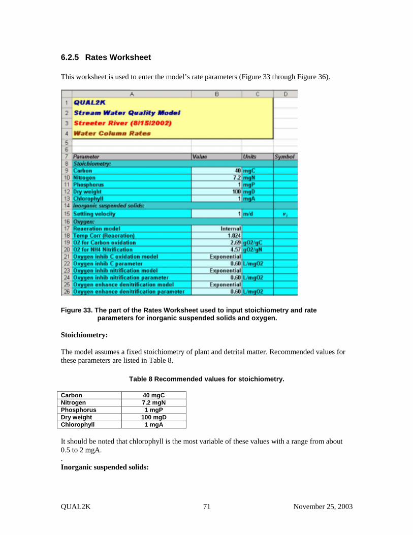
QUAL2K 71 November 25, 2003
6.2.5 Rates Worksheet This worksheet is used to enter the model’s rate parameters (Figure 33 through Figure 36).
Figure 33. The part of the Rates Worksheet used to input stoichiometry and rate
parameters for inorganic suspended solids and oxygen. Stoichiometry: The model assumes a fixed stoichiometry of plant and detrital matter. Recommended values for these parameters are listed in Table 8.
Table 8 Recommended values for stoichiometry. Carbon 40 mgC Nitrogen 7.2 mgN Phosphorus 1 mgP Dry weight 100 mgD Chlorophyll 1 mgA It should be noted that chlorophyll is the most variable of these values with a range from about 0.5 to 2 mgA. . Inorganic suspended solids:

QUAL2K 72 November 25, 2003
Settling velocity Oxygen: Reaeration model. Recall that the Reach Worksheet (Figure 31) can be used to specify the reaeration rate for each reach. Note that when the reaeration is entered this way, all other options are overridden. If reaeration is not specified on the Reach sheet, a pull-down menu (Figure 34) is used to select among several options to determine river reaeration:
• Internal. The reaeration is computed internally depending on the river’s depth and velocity (Covar 1976)
• O’Connor-Dobbins formula. • Churchill formula. • Owens-Gibbs formula.
The selected option will then be applied to all the unspecified cells.
Figure 34. The pull-down menu for global reaeration rates. Temperature correction (reaeration). Suggested value: 1.024. O2 for CBOD oxidation. Suggested value: 2.69 gO2/gC. O2 for NH4 nitrification. Suggested value: 4.57 gO2/gC. Oxygen inhibition C oxidation model. A pull-down menus is used to choose among the following options:
• Half-saturation • Exponential • Second order
Oxygen inhibition C parameter. This should be the proper parameter for the chosen oxygen inhibition model specified in cell B21. Oxygen inhibition nitrification model. A pull-down menus is used to choose among the following options:
• Half-saturation • Exponential • Second order
Oxygen inhibition nitrification parameter. This should be the proper parameter for the chosen oxygen inhibition model specified in cell B23. Oxygen enhancement denitrification model. A pull-down menus is used to choose among the following options:
• Half-saturation • Exponential • Second order
Oxygen enhancement denitrification parameter. This should be the proper parameter for the oxygen enhancement model specified in cell specified in cell B25.

QUAL2K 73 November 25, 2003
Figure 35. The part of the Rates Worksheet used to input rate parameters for slow CBOD,
fast CBOD, organic N, ammonium, nitrate, and organic P. Slow C: Hydrolysis rate Temperature correction Fast C: Oxidation rate Temperature correction Organic N: Hydrolysis Temperature correction Ammonium: Nitrification Temperature correction Nitrate: Denitrification Temperature correction Sediment denitrification transfer coefficient. This is the velocity at which nitrate diffuses into the sediments where it is denitrified to nitrogen gas. Temperature correction Organic P:

QUAL2K 74 November 25, 2003
Hydrolysis Temperature correction
Figure 36. The part of the Rates Worksheet used to input rate parameters for phytoplankton, bottom algae, detritus, pathogens and pH.
Floating Plants (Phytoplankton): Maximum Growth Rate Temperature correction Respiration Temperature correction Death Temperature correction Nitrogen half saturation constant Phosphorus half saturation constant Light model. A pull-down menu (Figure 37) is used to select among three light models:

QUAL2K 75 November 25, 2003
Figure 37. The pull-down menu to select the light model for phytoplankton growth. Light constant Ammonia preference Settling velocity Bottom algae: Maximum growth Temperature correction Respiration Temperature correction Death Temperature correction Nitrogen half saturation constant Phosphorus half saturation constant Light model. A pull-down menu identical to Figure 37 is used to select among three light models: Half saturation, Smith and Steele. Light Constant Ammonia preference Detritus (POM): Dissolution Temperature correction Settling Velocity Pathogens: Decay Temperature correction Settling Velocity pH: pCO2. The partial pressure of CO2 in the atmosphere (see Figure 20 for suggested values).

QUAL2K 76 November 25, 2003
6.2.6 Light and Heat Worksheet This worksheet is used to enter information related the system’s light and heat parameters.
Figure 38. The Light Worksheet used to input light-related parameters. Photosynthetically Available Radiation. This is the fraction of incoming solar radiation that is available for photosynthesis. It is recommended that this value be set to 0.47. Background light extinction. This parameter accounts for light extinction due to water and color. Linear chlorophyll light extinction. This parameter accounts for the linear dependence of light extinction due to phytoplankton chlorophyll a. According to Riley (1956), this parameter should be set to 0.0088/(m µgA/L). Nonlinear chlorophyll light extinction. This parameter accounts for the nonlinear dependence of light extinction due to phytoplankton chlorophyll a. According to Riley (1956), this parameter should be set to 0.054/(m (µgA/L)2/3). Note that if the relationship is believed to be linear, this parameter can be set to zero and the linear coefficient modified accordingly. Inorganic suspended solids light extinction. This parameter accounts for the nonlinear dependence of light extinction on inorganic suspended solids. Detritus light extinction. This parameter accounts for the nonlinear dependence of light extinction on detritus. Atmospheric attenuation model for solar (default: Bras). A pull down menu allows you to choose among 2 options: the Bras or the Ryan-Stolzenbach models. Atmospheric turbidity coefficient (2=clear, 5=smoggy, default=2). This is used if the Bras solar model is selected Atmospheric transmission coefficient (0.70-0.91, default 0.8). This is used if the Ryan-Stolzenbach solar model is selected.

QUAL2K 77 November 25, 2003
Atmospheric longwave emissivity model (default: Brutsaert). A pull down menu allows you to choose among 3 options: the Brutsaert, Brunt or Koberg models. Wind speed function for evaporation and air convection/conduction (default: Brady-Graves-Geyer). A pull down menu allows you to choose among 3 options: the Brady-Graves-Geyer, the Adams 1, or the Adams 2 models.

QUAL2K 78 November 25, 2003
6.2.7 Point Sources Worksheet This worksheet is used to enter information related the system’s point sources.
Figure 39. The Point Sources Worksheet. Name. User-specified label to identify the particular diffuse abstraction of inflow. Location. The kilometer where the point source or abstraction enters or leaves the river. Source Inflows and Outflows. A source can either be an inflow (loading or tributary) or an outflow (abstraction). Note that it can not be both. If there is an abstraction flow (i.e., a positive value in column C), the remaining information in columns D through T will be ignored.
Point abstraction. For an abstraction, a positive4 value for flow (m3/s) must be entered. If this is done, the values in columns D through T should be left blank. Point inflow. For an input, a value for flow (m3/s) must be entered in column D. Column C should be a zero or a blank.
Constituents. The temperature and the water quality concentrations of the inflow are entered in columns E through AZ.
QUAL2K allows the temperature and concentrations of each point source to be entered as a sinusoid that varies over the diel cycle. Figure 40 shows an example for the temperature of the Boulder CO WWTP.
19
21
6:00 12:00 18:00 0:00 6:00
Time of max = 17:13
Mean = 20.057
Range/2 = 0.717
20
4 Some software treats an abstraction as a negative inflow. In Q2K, the flow is entered as a positive number and the software internally calculates it as a loss from the reach.

QUAL2K 79 November 25, 2003
Figure 40. Temperature for the Boulder, CO wastewater treatment plant effluent on Sept.
21-22, 1987 along with a sinusoidal fit to the data.

QUAL2K 80 November 25, 2003
6.2.8 Diffuse Sources Worksheet This worksheet is used to enter information related the system’s diffuse (i.e., non-point) sources.
Figure 41. The Diffuse Sources Worksheet. Name. User-specified label to identify the particular diffuse abstraction of inflow. Location. The upstream and downstream kilometers over which the diffuse source or abstraction enters or leaves the river. Source inflows and outflows. A distributed source can either be an inflow (loading or tributary) or an outflow (abstraction). Note that it can not be both. If there is an abstraction flow (i.e., a positive value in column D), the remaining information in columns E through U will be ignored.
Diffuse abstraction. For an abstraction, a positive5 value for flow (m3/s) must be entered. If this is done, the values in columns U through U should be left blank. Diffuse inflow. For an input, a value for flow (m3/s) must be entered in column E. Column D should be a zero or a blank.
Constituents. The temperature and the water quality concentrations of the diffuse inflow are entered in columns F through U.
5 Some software treats an abstraction as a negative inflow. In Q2K, the flow is entered as a positive number and the software internally calculates it as a loss from the reach.
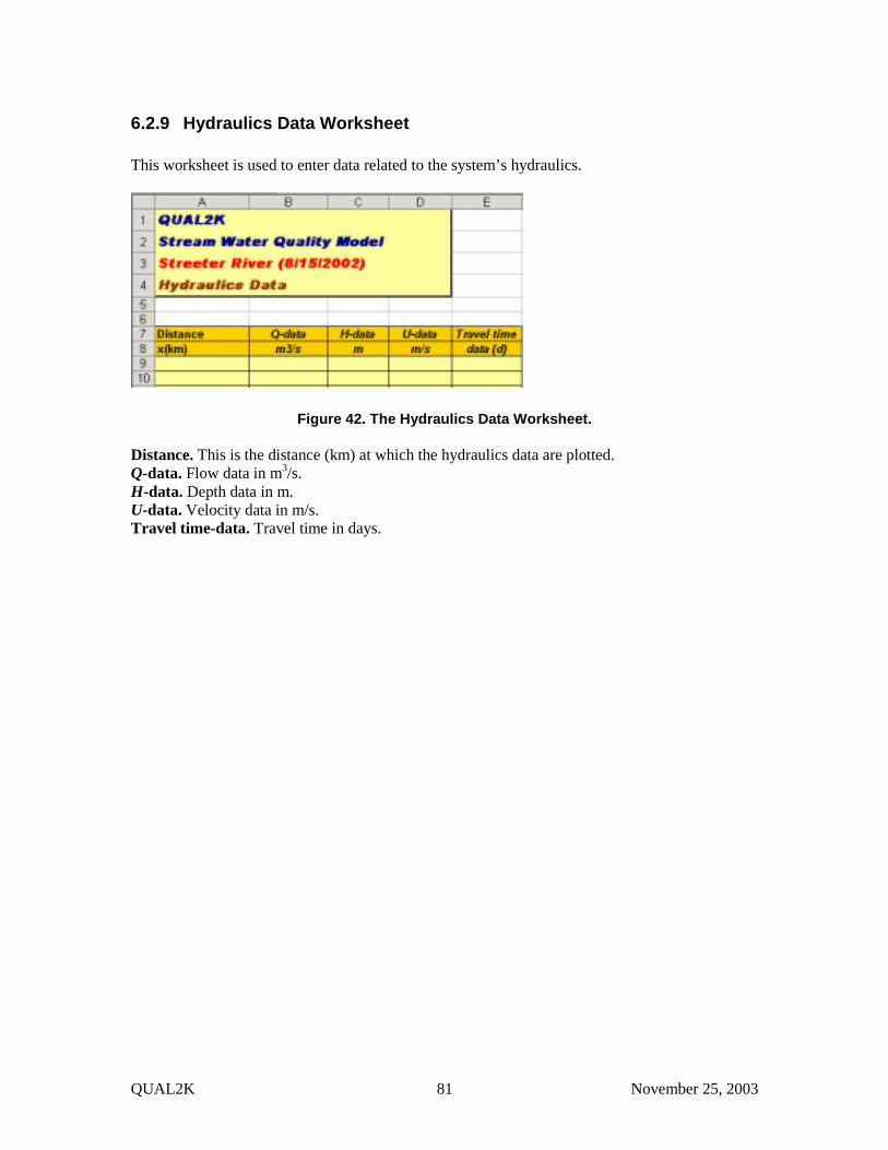
QUAL2K 81 November 25, 2003
6.2.9 Hydraulics Data Worksheet This worksheet is used to enter data related to the system’s hydraulics.
Figure 42. The Hydraulics Data Worksheet. Distance. This is the distance (km) at which the hydraulics data are plotted. Q-data. Flow data in m3/s. H-data. Depth data in m. U-data. Velocity data in m/s. Travel time-data. Travel time in days.

QUAL2K 82 November 25, 2003
6.2.10 Temperature Data Worksheet This worksheet is used to enter temperature data.
Figure 43. The Temperature Data Worksheet. Distance. This is the distance (km) at which the temperature data are plotted. Mean Temperature-data. The mean temperature in oC. Minimum Temperature-data. The minimum temperature in oC. Maximum Temperature-data. The maximum temperature in oC.

QUAL2K 83 November 25, 2003
6.2.11 WQ Data Worksheet This worksheet is used to enter mean daily values for water quality data. The first part of the worksheet is shown in Figure 44.
Figure 44. The first part of the Water Quality Data Worksheet. Distance. This is the distance (km) at which the water quality data are plotted. Constituents. The mean measured water quality concentrations are entered in columns B through R. Other Concentrations and Fluxes. A variety of other concentrations and fluxes are entered in Columns Q through AC as shown in Figure 45. These are
Bottom Algae. Total nitrogen-data. Total phosphorus-data. Total suspended solids-data. NH3 (unionized ammonia)-data % saturation-data. SOD-data Sediment ammonium flux. Sediment methane flux. Sediment inorganic phosphorus flux. Ultimate carbonaceous BOD. This is the total of detritus, slow CBOD, fast CBOD, and phytoplankton biomass expressed as oxygen equivalents. Total Organic Carbon. This is the total of inorganic suspended solids, phytoplankton biomass and detritus expressed as dry weight.
Figure 45. The last part of the Water Quality Data Worksheet.

QUAL2K 84 November 25, 2003
6.2.12 WQ Data Min Worksheet This worksheet is used to enter minimum daily values for water quality data. The layout is the same as for the WQ Data Worksheet.
6.2.13 WQ Data Max Worksheet This worksheet is used to enter maximum daily values for water quality data. The layout is the same as for the WQ Data Worksheet.

QUAL2K 85 November 25, 2003
6.2.14 Diel Data Worksheet This worksheet is used to enter diel data for a selected reach. This data is then plotted as points on the graphs of diel model output.
Figure 46. The Diel Data Worksheet.
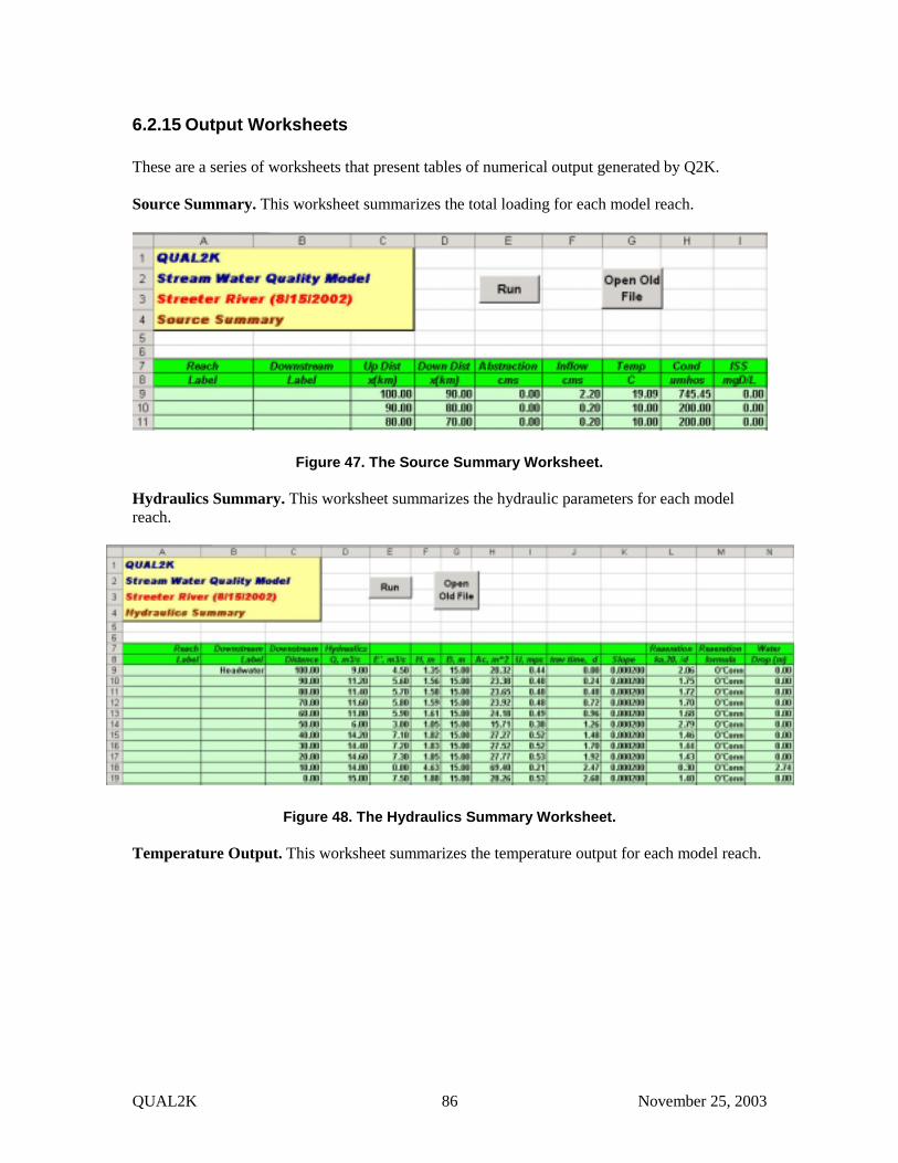
QUAL2K 86 November 25, 2003
6.2.15 Output Worksheets These are a series of worksheets that present tables of numerical output generated by Q2K. Source Summary. This worksheet summarizes the total loading for each model reach.
Figure 47. The Source Summary Worksheet. Hydraulics Summary. This worksheet summarizes the hydraulic parameters for each model reach.
Figure 48. The Hydraulics Summary Worksheet. Temperature Output. This worksheet summarizes the temperature output for each model reach.

QUAL2K 87 November 25, 2003
Figure 49. The Temperature Output Worksheet. WQ Output. This worksheet summarizes the mean concentration output for each model reach.
Figure 50. The first part of the Water Quality Output Worksheet.
Figure 51. The last part of the Water Quality Output Worksheet. WQ Min. This worksheet summarizes the minimum concentration output for each model reach. WQ Max. This worksheet summarizes the maximum concentration output for each model reach. Sediment Fluxes. This worksheet summarizes the fluxes of oxygen and nutrients between the water and the underlying sediment compartment for each model reach.

QUAL2K 88 November 25, 2003
Figure 52. The Sediment Flux Worksheet. Diel Output Worksheet. This worksheet displays diel output for temperature and water quality constituent data. Note that along with the water temperature, the temperature of the surface sediments are also displayed. In addition, the diel variation in total suspended solids, total phosphorus, total nitrogen, and oxygen saturation are also displayed.
Figure 53. The Diel Output Worksheet.

QUAL2K 89 November 25, 2003
6.2.16 Spatial Charts QUAL2K displays a series of charts that plot the model output and data versus distance (km) along the river.
Figure 54 shows an example of the plot for dissolved oxygen. The black line is the simulated mean DO (as displayed on the WQ Worksheet), whereas the dashed red lines are the minimum (WQ Min Worksheet) and maximum (WQ Max Worksheet) values, respectively. The black squares are the measured mean data points that were entered on the WQ Data Worksheet. The white squares are the minimum (WQ Min Worksheet) and maximum (WQ Max Worksheet) data points, respectively. The plot is labeled with the river name and the simulation date. Notice that this plot also displays the oxygen saturation as a dashed line.
Figure 54. The plot of dissolved oxygen versus distance downstream in km. The following series of variables are plotted: Hydraulics Plots:
• Travel Time • Flow • Velocity • Depth • Reaeration
Temperature and state-variable plots:

QUAL2K 90 November 25, 2003
• Temperature • Conductivity • ISS (Inorganic suspended solids) • Dissolved oxygen • Detritus • Slow CBOD • Fast CBOD • DON (Dissolved organic nitrogen) • NH4 (Ammonia nitrogen) • NO3 (Nitrate nitrogen) • DOP (Dissolved organic phosphorus) • Inorganic phosphorus • Phytoplankton • Bot Pl gD per m2 (Bottom algae in units of gD/m2) • Pathogen • Alkalinity • pH
Additional State-variable plots:
• Bot Pl mgA per m2 (Bottom algae in units of mgA/m2) • CBODu • NH3 • TN and TP • TSS
Sediment-water plots:
• SOD • CH4 Sed Flux • NH4 Sed Flux • Inorg P Sed Flux

QUAL2K 91 November 25, 2003
6.2.17 Diel Charts QUAL2K displays a series of charts that plot the model output and data versus time of day (in hours) for temperature and the model state variables.
Figure 55 shows an example of the diel plot for pH. The red line is the simulated pH (as displayed on the Diel Worksheet). The black squares are the measured data points that were entered on the Diel Data Worksheet. The plot is labeled with the river name, the date and the name of the reach that is plotted.
Figure 55. The diel plot of the Dissolved Oxygen versus time of day.


QUAL2K 93 November 25, 2003
7 REFERENCES Adams, E.E., D. J. Cosler, and K.R. Helfrich. 1987. "Analysis of evaporation data from heated
ponds", cs-5171, research project 2385-1, Electric Power Research Institute, Palo Alto, California 94304. April.
Andrews and Rodvey, 1980. Heat exchange between water and tidal flats. D.G.M 24(2). (in German)
Barnwell, T.O., Brown, L.C., and Mareck, W. 1989). Application of Expert Systems Technology in Water Quality Modeling. Water Sci. Tech. 21(8-9):1045-1056.
Bejan, A. 1993. Heat Transfer. Wiley, New York, NY. Bowie, G.L., Mills, W.B., Porcella, D.B., Campbell, C.L., Pagenkopf, J.R., Rupp, G.L., Johnson,
K.M., Chan, P.W.H., Gherini, S.A. and Chamberlin, C.E. 1985. Rates, Constants, and Kinetic Formulations in Surface Water Quality Modeling. U.S. Envir. Prot. Agency, ORD, Athens, GA, ERL, EPA/600/3-85/040.
Brady, D.K., Graves, W.L., and Geyer, J.C. 1969. Surface Heat Exchange at Power Plant Cooling Lakes, Cooling Water Discharge Project Report, No. 5, Edison Electric Inst. Pub. No. 69-901, New York, NY.
Bras, R.L. 1990. Hydrology. Addison-Wesley, Reading, MA. Brown, L.C., and Barnwell, T.O. 1987. The Enhanced Stream Water Quality Models QUAL2E
and QUAL2E-UNCAS, EPA/600/3-87-007, U.S. Environmental Protection Agency, Athens, GA, 189 pp.
Brunt, D. 1932. Notes on radiation in the atmosphere: I. Quart J Royal Meteorol Soc 58:389-420. Brutsaert, W. 1982. Evaporation into the atmosphere: theory, history, and applications. D.Reidel
Publishing Co., Hingham MA, 299 p. Butts, T. A. and Evans, R. L. 1983. Effects of Channel Dams on Dissolved Oxygen
Concentrations in Northeastern Illinois Streams, Circular 132, State of Illinois, Dept. of Reg. and Educ., Illinois Water Survey, Urbana, IL.
Carslaw, H.S. and Jaeger, J.C. 1959. Conduction of Heat in Solids, Oxford Press, Oxford, UK, 510 pp.
Cengel, Y.A. 1998 Heat Transfer: A Practical Approach. New York, McGraw-Hill. Chapra and Canale 2002. Numerical Methods for Engineers, 4th Ed. New York, McGraw-Hill. Chapra, S.C. 1997. Surface water quality modeling. New York, McGraw-Hill. Chow, V.T., Maidment, D.R., and Mays, L.W. 1988. Applied Hydrology. New York, McGraw-
Hill, 592 pp. Covar, A. P. 1976. "Selecting the Proper Reaeration Coefficient for Use in Water Quality
Models." Presented at the U.S. EPA Conference on Environmental Simulation and Modeling, April 19-22, 1976, Cincinnati, OH.
Di Toro, D. M. and J. F. Fitzpatrick. 1993. Chesapeake Bay sediment flux model. Tech. Report EL-93-2, U.S. Army Corps of Engineers, Waterways Experiment Station, Vicksburg, Mississippi, 316 pp.
Di Toro, D.M, Paquin, P.R., Subburamu, K. and Gruber, D.A. 1991. Sediment Oxygen Demand Model: Methane and Ammonia Oxidation. J. Environ. Eng., 116(5):945-986.
Di Toro, D.M. 1978. Optics of Turbid Estuarine Waters: Approximations and Applications. Water Res. 12:1059-1068.
Di Toro, D.M. 2001. Sediment Flux Modeling. Wiley-Interscience, New York, NY. Ecology. 2003. Shade.xls - a tool for estimating shade from riparian vegetation. Washington State
Department of Ecology. http://www.ecy.wa.gov/programs/eap/models/ Edinger, J.E., Brady, D.K., and Geyer, J.C. 1974. Heat Exchange and Transport in the
Environment. Report No. 14, EPRI Pub. No. EA-74-049-00-3, Electric Power Research Institute, Palo Alto, CA.

QUAL2K 94 November 25, 2003
Finnemore, E.J. and Franzini, J.B. 2002. Fluid Mechanics with Engineering Applications, 10th Ed. New York, McGraw, Hill.
Geiger, R. 1965. The climate near the ground. Harvard University Press. Cambridge, MA. Gordon, N.D, T.A. McMahon, and B.L. Finlayson. 1992. Stream Hydrology, An Introduction for
Ecologists. Published by John Wiley and Sons. Grigull, U. and Sandner, H. 1984. Heat Conduction. Springer-Verlag, New York, NY. Harbeck, G. E., 1962, A practical field technique for measuring reservoir evaporation utilizing
mass-transfer theory. US Geological Survey Professional Paper 272-E, 101-5. Harned, H.S., and Hamer, W.J. 1933. “The Ionization Constant of Water.” J. Am., Chem. Soc.
51:2194. Helfrich, K.R., E.E. Adams, A.L. Godbey, and D.R.F. Harleman. 1982. Evaluation of models for
predicting evaporative water loss in cooling impoundments. Report CS-2325, Research project 1260-17. Electric Power Research Institute, Pala Alto, CA. March 1982.
Hutchinson, G.E. 1957. A Treatise on Limnology, Vol. 1, Physics and Chemistry. Wiley, New York, NY.
Jobson, H.E. 1977. Bed Conduction Computation for Thermal Models. J. Hydraul. Div. ASCE. 103(10):1213-1217.
Koberg, G.E. 1964. Methods to compute long-wave radiation from the atmosphere and reflected solar radiation from a water surface. US Geological Survey Professional Paper 272-F.
Kreith, F. and Bohn, M.S. 1986. Principles of Heat Transfer, 4th Ed. Harper and Row, New York, NY.
Laws, E. A. and Chalup, M. S. 1990. A Microalgal Growth Model. Limnol. Oceanogr. 35(3):597-608.
LI-COR, 2003. Radiation Measurement Instruments, LI-COR, Lincoln, NE, 30 pp. Likens, G. E., and Johnson, N. M. (1969). "Measurements and analysis of the annual heat budget
for sediments of two Wisconsin lakes." Limnol. Oceanogr., 14(1):115-135. Mackay, D. and Yeun, A.T.K. 1983. Mass Transfer Coefficient Correlations for Volatilization of
Organic Solutes from Water. Environ. Sci. Technol. 17:211-233. Marciano, J.K. and G.E. Harbeck. 1952. Mass transfer studies in water loss investigation: Lake
Hefner studies. Geological Circular 229. U.S. Geological Survey, Washington DC. Meeus, J. 1999. Astronomical algorithms. Second edition. Willmann-Bell, Inc. Richmond, VA. Mills, A.F. 1992. Heat Transfer. Irwin, Homewood, IL. Nakshabandi, G.A. and H. Kohnke. 1965. Thermal conductivity and diffusivity of soils as related
to moisture tension and other physical properties. Agr. Met. Vol 2. Plummer, L.N. and Busenberg, E. 1982. The Solubilities of Calcite, Aragonite and Vaterite in
CO2-H2O Solutions Between 0 and 90 oC, and an Evaluation of the Aqueous Model for the System CaCO3−CO2−H2O. Geochim. Cosmochim. 46:1011-1040.
Raudkivi, A. I. 1979. Hydrology. Pergamon, Oxford, England. Redfield, A.C., Ketchum, B.H. and Richards, F.A. 1963. The Influence of Organisms on the
Composition of Seawater, in The Sea, M.N. Hill, ed. Vol. 2, pp. 27-46, Wiley-Interscience, NY.
Riley, G.A. 1956. Oceanography of Long Island Sound 1952-1954. II. Physical Oceanography, Bull. Bingham Oceanog. Collection 15, pp. 15-16.
Rosgen, D. 1996. Applied river morphology. Wildland Hydrology publishers. Pagosa Springs, CO.
Rutherford, J.C., Scarsbrook, M.R. and Broekhuizen, N. 2000. Grazer Control of Stream Algae: Modeling Temperature and Flood Effects. J. Environ. Eng. 126(4):331-339.
Ryan, P.J. and D.R.F. Harleman. 1971. Prediction of the annual cycle of temperature changes in a stratified lake or reservoir. Mathematical model and user’s manual. Ralph M. Parsons Laboratory Report No. 137. Massachusetts Institute of Technology. Cambridge, MA.

QUAL2K 95 November 25, 2003
Ryan, P.J. and K.D. Stolzenbach.1972. Engineering aspects of heat disposal from power generation, (D.R.F. Harleman, ed.). R.M. Parson Laboratory for Water Resources and Hydrodynamics, Department of Civil Engineering, Massachusetts Institute of Technology, Cambridge, MA
Shanahan, P. 1984. Water temperature modeling: a practical guide. In: Proceedings of stormwater and water quality model users group meeting, April 12-13, 1984. USEPA, EPA-600/9-85-003. (users.rcn.com/shanahan.ma.ultranet/TempModeling.pdf)
Stumm, W. and Morgan, J.J. 1996. Aquatic Chemistry, New York, Wiley-Interscience, 1022 pp. Thomann, R.V. and Mueller, J.A. 1987. Principles of Surface Water Quality Modeling and
Control. New York, Harper-Collins. TVA, 1972. Heat and mass transfer between a water surface and the atmosphere. Water
Resources Research, Laboratory Report No. 14. Engineering Laboratory, Division of Water Control Planning, Tennessee Valley Authority, Norris TN.
Wood, K.G. 1974. Carbon Dioxide Diffusivity Across the Air-Water Interface. Archiv für Hydrobiol. 73(1):57-69.


QUAL2K 97 November 25, 2003
8 APPENDIX A: NOMENCLATURE
Symbol Definition Units
iacresA , surface area of reach i acres
[CO2]s saturation concentration of carbon dioxide mole/L [CO3
2−] carbonate ion mole/L [H+] hydronium ion mole/L
[H2CO3*] sum of dissolved carbon dioxide and carbonic acid mole/L [HCO3
−] bicarbonate ion mole/L [OH−] hydroxyl ion mole/L
a velocity rating curve coefficient dimensionless a" mean atmospheric transmission coefficient after
scattering and absorption dimensionless
a’ mean atmospheric transmission coefficient dimensionless a1 atmospheric molecular scattering coefficient for radiation
transmission dimensionless
Aa atmospheric long-wave radiation coefficient dimensionless Ab atmospheric long-wave radiation coefficient mmHg-0.5
or mb-0.5 ab bottom algae gD/m2 Ac cross-sectional area m2 ad coefficient correcting dam reaeration for water quality dimensionless
Alk alkalinity eq L−1 or mgCaCO3/L
ap phytoplankton mgC/L ap phytoplankton concentration mgA/m3 at atmospheric attenuation dimensionless atc atmospheric transmission coefficient dimensionless B average reach width m b velocity rating curve exponent dimensionless B0 bottom width m bd coefficient correcting dam reaeration for dam type dimensionless c1 Bowen's coefficient 0.47 mmHg/oC cf fast reacting CBOD mgO2/L cf fast CBOD in the overlying water gO2/m3
Cgb(T) temperature-dependent maximum photosynthesis rate gD/(m2 d) CH4,1 methane concentration in the aerobic sediment layer gO2/m3
CL fraction of sky covered with clouds dimensionless cnps,i,j jth non-point source concentration for reach i oC
Cp specific heat of water cal/(g oC) cps,i,j jth point source concentration for reach i oC cs slowly reacting CBOD mgO2/L Cs saturation concentration of methane mgO2/L
CSOD the amount of oxygen demand generated by methane oxidation
gO2/m2/d
cT total inorganic carbon mole L−1 c'T,i−1 concentration of inorganic carbon entering reach below a
dam mgO2/L

QUAL2K 98 November 25, 2003
d dust attenuation coefficient dimensionless Dd pore water diffusion coefficient m2/d Dp diffusion coefficient for bioturbation m2/d E’i bulk dispersion coefficient between reaches i and i + 1 m3/d eair air vapor pressure mm Hg elev elevation above sea level m En numerical dispersion m2/d Ep,i longitudinal dispersion between reaches i and i + 1 m2/s
eqtime equation of time: the difference between mean solar time and true solar time when located on the reference longitude of the time zone considered
minutes
es saturation vapor pressure at water surface mmHg f photoperiod fraction of day
fdai fraction of ammonium in dissolved form in sediment layer i
dimensionless
fdpi fraction of inorganic phosphorus in dissolved form in sediment layer i
dimensionless
FLp phytoplankton growth attenuation due to light dimensionless Foxcf attenuation of CBOD oxidation due to low oxygen dimensionless Foxdn enhancement of denitrification at low oxygen
concentration dimensionless
Foxna attenuation due to low oxygen dimensionless Foxrb attenuation due to low oxygen dimensionless Foxrp attenuation due to low oxygen dimensionless fpai fraction of ammonium in particulate form in sediment
layer i dimensionless
fppi fraction of inorganic phosphorus in particulate form in sediment layer i
dimensionless
Fu fraction unionized ammonia g acceleration due to gravity = 9.81 m/s2
gX mass of element X g H water depth m H water depth m Hd drop in water elevation for a dam m Hi thickness of sediment layer i m
Hsed sediment thickness cm I(0) solar radiation at water surface cal/cm2/d I0 extraterrestrial radiation cal/cm2/d
Jan net atmospheric longwave radiation flux cal/(cm2 d) Jbr longwave back radiation flux from water cal/(cm2 d) Jc conduction flux cal/(cm2 d)
JC,G1 flux of labile dissolved carbon gO2/m2/d JCH4 Flux of methane from sediments to the overlying water gO2/m2/d JCH4,d flux of dissolved methane generated in anaerobic
sediments corrected for methane gas formation gO2/m2/d
JCH4,T carbon diagenesis flux corrected for denitrification gO2/m2/d Je evaporation flux cal/(cm2 d) Jh air-water heat flux cal/(cm2 d)

QUAL2K 99 November 25, 2003
JN nitrogen diagenesis flux gN/m2/d JO2,dn oxygen equivalents consumed during denitrification gO2/m2/d
JP phosphorus diagenesis flux gP/m2/d JPOC,G1 the flux of labile POC delivered to the anaerobic
sediment layer gO2/m2/d
JPOM the downward flux of POM gD m−2 d−1 Jsi sediment-water heat flux cal/(cm2 d) Jsn net solar shortwave radiation flux cal/(cm2 d)
k(T) temperature dependent first-order reaction rate /d K1 acidity constant for dissociation of carbonic acid K2 acidity constant for dissociation of bicarbonate Ka equilibrium coefficient for ammonium dissociation
ka(T) temperature-dependent oxygen reaeration coefficient /d kac(T) temperature-dependent carbon dioxide reaeration
coefficient /d
kdb(T) temperature-dependent bottom algae death rate /d kdc(T) temperature-dependent fast CBOD oxidation rate /d kdn(T) temperature-dependent denitrification rate /d kdp(T) temperature-dependent phytoplankton death rate /d kdt(T) temperature-dependent detritus dissolution rate /d kdx(T) temperature-dependent pathogen die-off rate /d
ke light extinction coefficient /m1 keb a background coefficient accounting for extinction due to
water and color /m
kgp(T) maximum photosynthesis rate at temperature T /d KH Henry's constant mole/(L atm)
khc(T) temperature-dependent slow CBOD hydrolysis rate /d khn(T) temperature-dependent organic nitrogen hydrolysis rate /d khnxb preference coefficient of bottom algae for ammonium mgN/m3 khnxp preference coefficient of phytoplankton for ammonium mgN/m3
khp(T) temperature-dependent organic phosphorus hydrolysis rate
/d
KL12 pore water diffusion mass transfer coefficient m/d KLb bottom algae light parameter KLp phytoplankton light parameter ly/d
KM,Dp oxygen half-saturation constant for bioturbation gO2/m3 kna(T) temperature-dependent nitrification rate for ammonia
nitrogen /d
KNH4 ammonium half-saturation constant gN/m3 KNH4,O2 oxygen half-saturation constant mgO2/L kPOC,G1 the mineralization rate of labile POC d−1 krb(T) temperature-dependent bottom algae respiration rate /d krp(T) temperature-dependent phytoplankton respiration rate /d ksNb nitrogen half-saturation constant for bottom algae µgN/L ksNp nitrogen half-saturation constant for phytoplankton µgN/L Ksocf parameter for oxygen dependency of fast CBOD
oxidation
Ksodn parameter for oxygen dependency of denitrification

QUAL2K 100 November 25, 2003
Ksona parameter for oxygen dependency of nitrification ksPb phosphorus half-saturation constant for bottom algae µgP/L ksPp phosphorus half-saturation constant for phytoplankton µgP/L Kw acidity constant for dissociation of water Lat latitude radians Llm longitude of local meridian degrees
localTime local standard time minutes Lsm longitude of standard meridian degrees m optical air mass dimensionless
mgY mass of element Y mg mi inorganic suspended solids mgD/L mi the solids concentration in sediment layer i gD/m3 mo detritus mgD/L mo detritus concentration gD/m3 n Manning roughness coefficient na ammonia nitrogen mgN/L na the ammonium concentration in the overlying water mgN/m3 nau unionized ammonia nitrogen mgN/L nfac atmospheric turbidity factor dimensionless
NH4,i the concentration of total ammonium in sediment layer i gN/m3 nn nitrate nitrogen mgN/L nn nitrate concentration in the overlying water mgN/m3 no dissolved organic nitrogen mgN/L
NO3,i nitrate concentration in layer i gN/m3 npai total number of non-point abstractions outflows from
reach i dimensionless
npsi total number of non-point sources inflows to reach i dimensionless NSOD the amount of oxygen demand generated by nitrification gO2/m2/d
o dissolved oxygen mgO2/L o the dissolved oxygen concentration in the overlying
water gO2/m3
o’i−1 oxygen concentration entering a reach below a dam mgO2/L ocrit critical oxygen concentration for sediment phosphorus
sorption gO2/m3
os(T, elev) saturation concentration of oxygen at temperature, T, and elevation above sea level, elev
mgO2/L
P wetted perimeter m Pab preference for ammonium as a nitrogen source for
bottom algae dimensionless
pai total number of point abstractions from reach i dimensionless Pap preference for ammonium as a nitrogen source for
phytoplankton dimensionless
PAR(z) photosynthetically available radiation (PAR) at depth z below water surface
ly/d
patm atmospheric pressure mm Hg pCO2 atmospheric partial pressure of carbon dioxide atm
pi inorganic phosphorus µgP/L pi the inorganic phosphorus in the overlying water mgP/m3 po dissolved organic phosphorus µgP/L
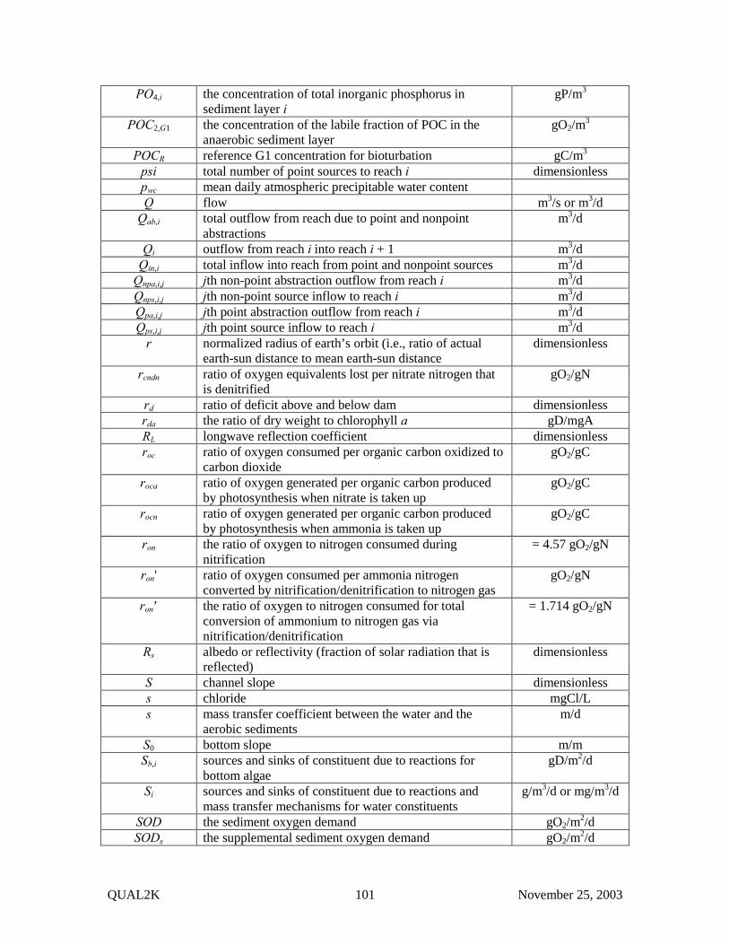
QUAL2K 101 November 25, 2003
PO4,i the concentration of total inorganic phosphorus in sediment layer i
gP/m3
POC2,G1 the concentration of the labile fraction of POC in the anaerobic sediment layer
gO2/m3
POCR reference G1 concentration for bioturbation gC/m3 psi total number of point sources to reach i dimensionless pwc mean daily atmospheric precipitable water content Q flow m3/s or m3/d
Qab,i total outflow from reach due to point and nonpoint abstractions
m3/d
Qi outflow from reach i into reach i + 1 m3/d Qin,i total inflow into reach from point and nonpoint sources m3/d
Qnpa,i,j jth non-point abstraction outflow from reach i m3/d Qnps,i,j jth non-point source inflow to reach i m3/d Qpa,i,j jth point abstraction outflow from reach i m3/d Qps,i,j jth point source inflow to reach i m3/d
r normalized radius of earth’s orbit (i.e., ratio of actual earth-sun distance to mean earth-sun distance
dimensionless
rcndn ratio of oxygen equivalents lost per nitrate nitrogen that is denitrified
gO2/gN
rd ratio of deficit above and below dam dimensionless rda the ratio of dry weight to chlorophyll a gD/mgA RL longwave reflection coefficient dimensionless roc ratio of oxygen consumed per organic carbon oxidized to
carbon dioxide gO2/gC
roca ratio of oxygen generated per organic carbon produced by photosynthesis when nitrate is taken up
gO2/gC
rocn ratio of oxygen generated per organic carbon produced by photosynthesis when ammonia is taken up
gO2/gC
ron the ratio of oxygen to nitrogen consumed during nitrification
= 4.57 gO2/gN
ron' ratio of oxygen consumed per ammonia nitrogen converted by nitrification/denitrification to nitrogen gas
gO2/gN
ron’ the ratio of oxygen to nitrogen consumed for total conversion of ammonium to nitrogen gas via nitrification/denitrification
= 1.714 gO2/gN
Rs albedo or reflectivity (fraction of solar radiation that is reflected)
dimensionless
S channel slope dimensionless s chloride mgCl/L s mass transfer coefficient between the water and the
aerobic sediments m/d
S0 bottom slope m/m Sb,i sources and sinks of constituent due to reactions for
bottom algae gD/m2/d
Si sources and sinks of constituent due to reactions and mass transfer mechanisms for water constituents
g/m3/d or mg/m3/d
SOD the sediment oxygen demand gO2/m2/d SODs the supplemental sediment oxygen demand gO2/m2/d

QUAL2K 102 November 25, 2003
SODt total sediment oxygen demand = SOD + SODs gO2/m2/d ss channel side slope m/m t time d T water temperature oC T water temperature oC
T,w,f water temperature oF Ta absolute temperature K Tair air temperature oC Tair,f air temperature oF Td dew-point temperature oC
Ti temperature in reach i oC timezone time zone indicates local time zone in relation to
Greenwich Mean Time (GMT) (negative in western hemisphere)
hours
Tnps,i,j jth non-point source temperature for reach i oC Tps,i,j jth point source temperature for reach i oC
trueSolarTime time determined from actual position of the sun in the sky
minutes
Ts,i temperature of bottom sediment oC tsr time of sunrise Hr tss time of sunset Hr
Tstd standard time Hr tt,i travel time from headwater to end of reach i D U mean velocity m/s
Ui* shear velocity m/s Uw wind speed m/s
Uw,mph wind speed mph Uw,z wind speed at height zw above water surface m/s va phytoplankton settling velocity m/d va phytoplankton settling velocity m/d vdt detritus settling velocity m/d vdt detritus settling velocity m/d vi inorganic suspended solids settling velocity m/d Vi volume of ith reach m3 vp pathogen settling velocity m/d vpc non-living particulate organic carbon settling velocity m/d W0 solar constant 2851 cal/cm2/d w2 the burial velocity m/d
Wh,i net heat load from point and non-point sources into reach i
cal/d
Wi external loading of constituent to reach i g/d or mg/d x pathogen cfu/100 mL zw height above water for wind speed measurements m

QUAL2K 103 November 25, 2003
Greek:
Symbol Definition Units α depth rating curve coefficient dimensionless α sun’s altitude radians αd sun’s altitude degrees αs sediment thermal diffusivity cm2/s α0 fraction of total inorganic carbon in carbon dioxide dimensionless α1 fraction of total inorganic carbon in bicarbonate dimensionless α2 fraction of total inorganic carbon in carbonate dimensionless αi effect of inorganic suspended solids on light attenuation L/mgD/m αo effect of particulate organic matter on light attenuation L/mgD/m αp linear effect of chlorophyll on light attenuation L/µgA/m αpn non-linear effect of chlorophyll on light attenuation (L/µgA)2/3/m β depth rating curve exponent dimensionless δ solar declination radians
∆πPO4,1 factor that increases the aerobic sediment layer partition coefficient relative to the anaerobic coefficient
dimensionless
vθ∆ virtual temperature difference between the water and air °F
∆ts difference between standard and local civic time hr ∆xi length of ith reach m
ε emissivity of water dimensionless εclear emissivity of longwave radiation from the sky with no
clouds 0-1
εsky emissivity of longwave radiation from the sky with clouds
0-1
εa estimated error % φLb bottom algae light attenuation 0-1 φLp phytoplankton light attenuation 0-1 φNb bottom algae nutrient attenuation factor 0-1 φNp phytoplankton nutrient attenuation factor 0-1 µp phytoplankton photosynthesis rate /d ρ density of water g/cm3 σ Stefan-Boltzmann constant 11.7x10⁻⁸ cal/(cm2 d K4) τ local hour angle of sun radians τi residence time of ith reach d θ temperature coefficient for zero and first-order reactions dimensionless θam elevation adjusted optical air mass ω12 the bioturbation mass transfer coefficient between the
sediment layers m/d
πai the partition coefficient for ammonium in sediment layer i
m3/gD
πpi the partition coefficient for inorganic phosphorus in sediment layer i
m3/gD
θCH4 temperature correction factor for sediment methane oxidation
dimensionless

QUAL2K 104 November 25, 2003
θDd temperature coefficient for porewater diffusion dimensionless θDp temperature coefficient for bioturbation diffusion dimensionless θNH4 temperature correction factor for sediment nitrification dimensionless θNO3 sediment denitrification temperature correction factor dimensionless
θPOC,G1 temperature correction factor for labile POC mineralization
dimensionless
κCH4,1 the reaction velocity for methane oxidation in the aerobic sediments
m/d
κNH4,1 the reaction velocity for nitrification in the aerobic sediments
m/d
κNO3,i denitrification reaction velocity sediment layer i m/d

QUAL2K 105 November 25, 2003
9 APPENDIX B: SOLAR POSITION, SUNRISE, AND SUNSET CALCULATIONS
The sunrise/sunset and solar position functions are a VBA translation of NOAA's sunrise/sunset calculator and NOAA's solar position calculator at the following web pages:
• http://www.srrb.noaa.gov/highlights/sunrise/sunrise.html • http://www.srrb.noaa.gov/highlights/sunrise/azel.html
The calculations in the NOAA Sunrise/Sunset and Solar Position Calculators are based on equations from Astronomical Algorithms, by Jean Meeus.The sunrise and sunset results have been verified by NOAA to be accurate to within a minute for locations between +/- 72° latitude, and within 10 minutes outside of those latitudes. Five main functions are included for use from Excel worksheets or VBA programs:
• sunrise(lat, lon, year, month, day, timezone, dlstime) calculates the local time of sunrise for a location and date
• solarnoon(lat, lon, year, month, day, timezone, dlstime) calculates the local time of solar noon for a location and date (the time when the sun crosses the meridian)
• sunset(lat, lon, year, month, day, timezone, dlstime) calculates the local time of sunset for a location and date
• solarazimuth(lat, lon, year, month, day, hour, minute, second, timezone, dlstime) calculates the solar azimuth for a location, date, and time (degrees clockwise from north to the point on the horizon directly below the sun)
• solarelevation(lat, lon, year, month, day, hour, minute, second, timezone, dlstime) calculates the solar elevation for a location, date, and time (degrees vertically from horizon to the sun)
The sign convention for the main functions and subroutine is:
• positive latitude decimal degrees for northern hemisphere • negative longitude degrees for western hemisphere • negative time zone hours for western hemisphere
The Excel/VBA functions and subroutines for solar position, sunrise, and sunset times are as follows:
Option Explicit
Function radToDeg(angleRad)'// Convert radian angle to degrees
radToDeg = (180# * angleRad / Application.WorksheetFunction.Pi())
End Function
Function degToRad(angleDeg)'// Convert degree angle to radians
degToRad = (Application.WorksheetFunction.Pi() * angleDeg / 180#)
End Function
Function calcJD(year, month, day)
'***********************************************************************/'* Name: calcJD'* Type: Function'* Purpose: Julian day from calendar day'* Arguments:'* year : 4 digit year

QUAL2K 106 November 25, 2003
'* month: January = 1'* day : 1 - 31'* Return value:'* The Julian day corresponding to the date'* Note:'* Number is returned for start of day. Fractional days should be'* added later.'***********************************************************************/
Dim A As Double, B As Double, jd As Double
If (month <= 2) Thenyear = year - 1month = month + 12
End If
A = Application.WorksheetFunction.Floor(year / 100, 1)B = 2 - A + Application.WorksheetFunction.Floor(A / 4, 1)
jd = Application.WorksheetFunction.Floor(365.25 * (year + 4716), 1) + _Application.WorksheetFunction.Floor(30.6001 * (month + 1), 1) + day + B - 1524.5
calcJD = jd
'gp put the year and month back where they belongIf month = 13 Thenmonth = 1year = year + 1
End IfIf month = 14 Thenmonth = 2year = year + 1
End If
End Function
Function calcTimeJulianCent(jd)
'***********************************************************************/'* Name: calcTimeJulianCent'* Type: Function'* Purpose: convert Julian Day to centuries since J2000.0.'* Arguments:'* jd : the Julian Day to convert'* Return value:'* the T value corresponding to the Julian Day'***********************************************************************/
Dim t As Double
t = (jd - 2451545#) / 36525#calcTimeJulianCent = t
End Function
Function calcJDFromJulianCent(t)
'***********************************************************************/'* Name: calcJDFromJulianCent'* Type: Function'* Purpose: convert centuries since J2000.0 to Julian Day.'* Arguments:'* t : number of Julian centuries since J2000.0'* Return value:'* the Julian Day corresponding to the t value'***********************************************************************/
Dim jd As Double
jd = t * 36525# + 2451545#calcJDFromJulianCent = jd
End Function
Function calcGeomMeanLongSun(t)
'***********************************************************************/'* Name: calGeomMeanLongSun'* Type: Function'* Purpose: calculate the Geometric Mean Longitude of the Sun'* Arguments:'* t : number of Julian centuries since J2000.0

QUAL2K 107 November 25, 2003
'* Return value:'* the Geometric Mean Longitude of the Sun in degrees'***********************************************************************/
Dim l0 As Double
l0 = 280.46646 + t * (36000.76983 + 0.0003032 * t)Do
If (l0 <= 360) And (l0 >= 0) Then Exit DoIf l0 > 360 Then l0 = l0 - 360If l0 < 0 Then l0 = l0 + 360
Loop
calcGeomMeanLongSun = l0
End Function
Function calcGeomMeanAnomalySun(t)
'***********************************************************************/'* Name: calGeomAnomalySun'* Type: Function'* Purpose: calculate the Geometric Mean Anomaly of the Sun'* Arguments:'* t : number of Julian centuries since J2000.0'* Return value:'* the Geometric Mean Anomaly of the Sun in degrees'***********************************************************************/
Dim m As Double
m = 357.52911 + t * (35999.05029 - 0.0001537 * t)calcGeomMeanAnomalySun = m
End Function
Function calcEccentricityEarthOrbit(t)
'***********************************************************************/'* Name: calcEccentricityEarthOrbit'* Type: Function'* Purpose: calculate the eccentricity of earth's orbit'* Arguments:'* t : number of Julian centuries since J2000.0'* Return value:'* the unitless eccentricity'***********************************************************************/
Dim e As Double
e = 0.016708634 - t * (0.000042037 + 0.0000001267 * t)calcEccentricityEarthOrbit = e
End Function
Function calcSunEqOfCenter(t)
'***********************************************************************/'* Name: calcSunEqOfCenter'* Type: Function'* Purpose: calculate the equation of center for the sun'* Arguments:'* t : number of Julian centuries since J2000.0'* Return value:'* in degrees'***********************************************************************/
Dim m As Double, mrad As Double, sinm As Double, sin2m As Double, sin3m As DoubleDim c As Double
m = calcGeomMeanAnomalySun(t)
mrad = degToRad(m)sinm = Sin(mrad)sin2m = Sin(mrad + mrad)sin3m = Sin(mrad + mrad + mrad)
c = sinm * (1.914602 - t * (0.004817 + 0.000014 * t)) _+ sin2m * (0.019993 - 0.000101 * t) + sin3m * 0.000289
calcSunEqOfCenter = c

QUAL2K 108 November 25, 2003
End Function
Function calcSunTrueLong(t)
'***********************************************************************/'* Name: calcSunTrueLong'* Type: Function'* Purpose: calculate the true longitude of the sun'* Arguments:'* t : number of Julian centuries since J2000.0'* Return value:'* sun's true longitude in degrees'***********************************************************************/
Dim l0 As Double, c As Double, O As Double
l0 = calcGeomMeanLongSun(t)c = calcSunEqOfCenter(t)
O = l0 + ccalcSunTrueLong = O
End Function
Function calcSunTrueAnomaly(t)
'***********************************************************************/'* Name: calcSunTrueAnomaly (not used by sunrise, solarnoon, sunset)'* Type: Function'* Purpose: calculate the true anamoly of the sun'* Arguments:'* t : number of Julian centuries since J2000.0'* Return value:'* sun's true anamoly in degrees'***********************************************************************/
Dim m As Double, c As Double, v As Double
m = calcGeomMeanAnomalySun(t)c = calcSunEqOfCenter(t)
v = m + ccalcSunTrueAnomaly = v
End Function
Function calcSunRadVector(t)
'***********************************************************************/'* Name: calcSunRadVector (not used by sunrise, solarnoon, sunset)'* Type: Function'* Purpose: calculate the distance to the sun in AU'* Arguments:'* t : number of Julian centuries since J2000.0'* Return value:'* sun radius vector in AUs'***********************************************************************/
Dim v As Double, e As Double, r As Double
v = calcSunTrueAnomaly(t)e = calcEccentricityEarthOrbit(t)
r = (1.000001018 * (1 - e * e)) / (1 + e * Cos(degToRad(v)))calcSunRadVector = r
End Function
Function calcSunApparentLong(t)
'***********************************************************************/'* Name: calcSunApparentLong (not used by sunrise, solarnoon, sunset)'* Type: Function'* Purpose: calculate the apparent longitude of the sun'* Arguments:'* t : number of Julian centuries since J2000.0'* Return value:'* sun's apparent longitude in degrees'***********************************************************************/

QUAL2K 109 November 25, 2003
Dim O As Double, omega As Double, lambda As Double
O = calcSunTrueLong(t)
omega = 125.04 - 1934.136 * tlambda = O - 0.00569 - 0.00478 * Sin(degToRad(omega))calcSunApparentLong = lambda
End Function
Function calcMeanObliquityOfEcliptic(t)
'***********************************************************************/'* Name: calcMeanObliquityOfEcliptic'* Type: Function'* Purpose: calculate the mean obliquity of the ecliptic'* Arguments:'* t : number of Julian centuries since J2000.0'* Return value:'* mean obliquity in degrees'***********************************************************************/
Dim seconds As Double, e0 As Double
seconds = 21.448 - t * (46.815 + t * (0.00059 - t * (0.001813)))e0 = 23# + (26# + (seconds / 60#)) / 60#calcMeanObliquityOfEcliptic = e0
End Function
Function calcObliquityCorrection(t)
'***********************************************************************/'* Name: calcObliquityCorrection'* Type: Function'* Purpose: calculate the corrected obliquity of the ecliptic'* Arguments:'* t : number of Julian centuries since J2000.0'* Return value:'* corrected obliquity in degrees'***********************************************************************/
Dim e0 As Double, omega As Double, e As Double
e0 = calcMeanObliquityOfEcliptic(t)
omega = 125.04 - 1934.136 * te = e0 + 0.00256 * Cos(degToRad(omega))calcObliquityCorrection = e
End Function
Function calcSunRtAscension(t)
'***********************************************************************/'* Name: calcSunRtAscension (not used by sunrise, solarnoon, sunset)'* Type: Function'* Purpose: calculate the right ascension of the sun'* Arguments:'* t : number of Julian centuries since J2000.0'* Return value:'* sun's right ascension in degrees'***********************************************************************/
Dim e As Double, lambda As Double, tananum As Double, tanadenom As DoubleDim alpha As Double
e = calcObliquityCorrection(t)lambda = calcSunApparentLong(t)
tananum = (Cos(degToRad(e)) * Sin(degToRad(lambda)))tanadenom = (Cos(degToRad(lambda)))
'original NOAA code using javascript Math.Atan2(y,x) convention:' var alpha = radToDeg(Math.atan2(tananum, tanadenom));' alpha = radToDeg(Application.WorksheetFunction.Atan2(tananum, tanadenom))
'translated using Excel VBA Application.WorksheetFunction.Atan2(x,y) convention:alpha = radToDeg(Application.WorksheetFunction.Atan2(tanadenom, tananum))
calcSunRtAscension = alpha
QUAL2K 110 November 25, 2003
End Function
Function calcSunDeclination(t)
'***********************************************************************/'* Name: calcSunDeclination'* Type: Function'* Purpose: calculate the declination of the sun'* Arguments:'* t : number of Julian centuries since J2000.0'* Return value:'* sun's declination in degrees'***********************************************************************/
Dim e As Double, lambda As Double, sint As Double, theta As Double
e = calcObliquityCorrection(t)lambda = calcSunApparentLong(t)
sint = Sin(degToRad(e)) * Sin(degToRad(lambda))theta = radToDeg(Application.WorksheetFunction.Asin(sint))calcSunDeclination = theta
End Function
Function calcEquationOfTime(t)
'***********************************************************************/'* Name: calcEquationOfTime'* Type: Function'* Purpose: calculate the difference between true solar time and mean'* solar time'* Arguments:'* t : number of Julian centuries since J2000.0'* Return value:'* equation of time in minutes of time'***********************************************************************/
Dim epsilon As Double, l0 As Double, e As Double, m As DoubleDim y As Double, sin2l0 As Double, sinm As DoubleDim cos2l0 As Double, sin4l0 As Double, sin2m As Double, Etime As Double
epsilon = calcObliquityCorrection(t)l0 = calcGeomMeanLongSun(t)e = calcEccentricityEarthOrbit(t)m = calcGeomMeanAnomalySun(t)
y = Tan(degToRad(epsilon) / 2#)y = y ^ 2
sin2l0 = Sin(2# * degToRad(l0))sinm = Sin(degToRad(m))cos2l0 = Cos(2# * degToRad(l0))sin4l0 = Sin(4# * degToRad(l0))sin2m = Sin(2# * degToRad(m))
Etime = y * sin2l0 - 2# * e * sinm + 4# * e * y * sinm * cos2l0 _- 0.5 * y * y * sin4l0 - 1.25 * e * e * sin2m
calcEquationOfTime = radToDeg(Etime) * 4#
End Function
Function calcHourAngleSunrise(lat, SolarDec)
'***********************************************************************/'* Name: calcHourAngleSunrise'* Type: Function'* Purpose: calculate the hour angle of the sun at sunrise for the'* latitude'* Arguments:'* lat : latitude of observer in degrees'* solarDec : declination angle of sun in degrees'* Return value:'* hour angle of sunrise in radians'***********************************************************************/
Dim latrad As Double, sdRad As Double, HAarg As Double, HA As Double
latrad = degToRad(lat)
QUAL2K 111 November 25, 2003
sdRad = degToRad(SolarDec)
HAarg = (Cos(degToRad(90.833)) / (Cos(latrad) * Cos(sdRad)) - Tan(latrad) * Tan(sdRad))
HA = (Application.WorksheetFunction.Acos(Cos(degToRad(90.833)) _/ (Cos(latrad) * Cos(sdRad)) - Tan(latrad) * Tan(sdRad)))
calcHourAngleSunrise = HA
End Function
Function calcHourAngleSunset(lat, SolarDec)
'***********************************************************************/'* Name: calcHourAngleSunset'* Type: Function'* Purpose: calculate the hour angle of the sun at sunset for the'* latitude'* Arguments:'* lat : latitude of observer in degrees'* solarDec : declination angle of sun in degrees'* Return value:'* hour angle of sunset in radians'***********************************************************************/
Dim latrad As Double, sdRad As Double, HAarg As Double, HA As Double
latrad = degToRad(lat)sdRad = degToRad(SolarDec)
HAarg = (Cos(degToRad(90.833)) / (Cos(latrad) * Cos(sdRad)) - Tan(latrad) * Tan(sdRad))
HA = (Application.WorksheetFunction.Acos(Cos(degToRad(90.833)) _/ (Cos(latrad) * Cos(sdRad)) - Tan(latrad) * Tan(sdRad)))
calcHourAngleSunset = -HA
End Function
Function calcSunriseUTC(jd, Latitude, longitude)
'***********************************************************************/'* Name: calcSunriseUTC'* Type: Function'* Purpose: calculate the Universal Coordinated Time (UTC) of sunrise'* for the given day at the given location on earth'* Arguments:'* JD : julian day'* latitude : latitude of observer in degrees'* longitude : longitude of observer in degrees'* Return value:'* time in minutes from zero Z'***********************************************************************/
Dim t As Double, eqtime As Double, SolarDec As Double, hourangle As DoubleDim delta As Double, timeDiff As Double, timeUTC As DoubleDim newt As Double
t = calcTimeJulianCent(jd)
' // *** First pass to approximate sunrise
eqtime = calcEquationOfTime(t)SolarDec = calcSunDeclination(t)hourangle = calcHourAngleSunrise(Latitude, SolarDec)
delta = longitude - radToDeg(hourangle)timeDiff = 4 * delta
' in minutes of timetimeUTC = 720 + timeDiff - eqtime
' in minutes
' *** Second pass includes fractional jday in gamma calc
newt = calcTimeJulianCent(calcJDFromJulianCent(t) + timeUTC / 1440#)eqtime = calcEquationOfTime(newt)SolarDec = calcSunDeclination(newt)hourangle = calcHourAngleSunrise(Latitude, SolarDec)delta = longitude - radToDeg(hourangle)timeDiff = 4 * deltatimeUTC = 720 + timeDiff - eqtime

QUAL2K 112 November 25, 2003
' in minutes
calcSunriseUTC = timeUTC
End Function
Function calcSolNoonUTC(t, longitude)
'***********************************************************************/'* Name: calcSolNoonUTC'* Type: Function'* Purpose: calculate the Universal Coordinated Time (UTC) of solar'* noon for the given day at the given location on earth'* Arguments:'* t : number of Julian centuries since J2000.0'* longitude : longitude of observer in degrees'* Return value:'* time in minutes from zero Z'***********************************************************************/
Dim newt As Double, eqtime As Double, solarNoonDec As Double, solNoonUTC As Double
newt = calcTimeJulianCent(calcJDFromJulianCent(t) + 0.5 + longitude / 360#)
eqtime = calcEquationOfTime(newt)solarNoonDec = calcSunDeclination(newt)solNoonUTC = 720 + (longitude * 4) - eqtime
calcSolNoonUTC = solNoonUTC
End Function
Function calcSunsetUTC(jd, Latitude, longitude)
'***********************************************************************/'* Name: calcSunsetUTC'* Type: Function'* Purpose: calculate the Universal Coordinated Time (UTC) of sunset'* for the given day at the given location on earth'* Arguments:'* JD : julian day'* latitude : latitude of observer in degrees'* longitude : longitude of observer in degrees'* Return value:'* time in minutes from zero Z'***********************************************************************/
Dim t As Double, eqtime As Double, SolarDec As Double, hourangle As DoubleDim delta As Double, timeDiff As Double, timeUTC As DoubleDim newt As Double
t = calcTimeJulianCent(jd)
' // First calculates sunrise and approx length of day
eqtime = calcEquationOfTime(t)SolarDec = calcSunDeclination(t)hourangle = calcHourAngleSunset(Latitude, SolarDec)
delta = longitude - radToDeg(hourangle)timeDiff = 4 * deltatimeUTC = 720 + timeDiff - eqtime
' // first pass used to include fractional day in gamma calc
newt = calcTimeJulianCent(calcJDFromJulianCent(t) + timeUTC / 1440#)eqtime = calcEquationOfTime(newt)SolarDec = calcSunDeclination(newt)hourangle = calcHourAngleSunset(Latitude, SolarDec)
delta = longitude - radToDeg(hourangle)timeDiff = 4 * deltatimeUTC = 720 + timeDiff - eqtime
' // in minutes
calcSunsetUTC = timeUTC
End Function
Function sunrise(lat, lon, year, month, day, timezone, dlstime)

QUAL2K 113 November 25, 2003
'***********************************************************************/'* Name: sunrise'* Type: Main Function called by spreadsheet'* Purpose: calculate time of sunrise for the entered date'* and location.'* For latitudes greater than 72 degrees N and S, calculations are'* accurate to within 10 minutes. For latitudes less than +/- 72°'* accuracy is approximately one minute.'* Arguments:' latitude = latitude (decimal degrees)' longitude = longitude (decimal degrees)' NOTE: longitude is negative for western hemisphere for input cells' in the spreadsheet for calls to the functions named' sunrise, solarnoon, and sunset. Those functions convert the' longitude to positive for the western hemisphere for calls to' other functions using the original sign convention' from the NOAA javascript code.' year = year' month = month' day = day' timezone = time zone hours relative to GMT/UTC (hours)' dlstime = daylight savings time (0 = no, 1 = yes) (hours)'* Return value:'* sunrise time in local time (days)'***********************************************************************/
Dim longitude As Double, Latitude As Double, jd As DoubleDim riseTimeGMT As Double, riseTimeLST As Double
' change sign convention for longitude from negative to positive in western hemispherelongitude = lon * -1Latitude = latIf (Latitude > 89.8) Then Latitude = 89.8If (Latitude < -89.8) Then Latitude = -89.8
jd = calcJD(year, month, day)
' // Calculate sunrise for this dateriseTimeGMT = calcSunriseUTC(jd, Latitude, longitude)
' // adjust for time zone and daylight savings time in minutesriseTimeLST = riseTimeGMT + (60 * timezone) + (dlstime * 60)
' // convert to dayssunrise = riseTimeLST / 1440
End Function
Function solarnoon(lat, lon, year, month, day, timezone, dlstime)
'***********************************************************************/'* Name: solarnoon'* Type: Main Function called by spreadsheet'* Purpose: calculate the Universal Coordinated Time (UTC) of solar'* noon for the given day at the given location on earth'* Arguments:' year' month' day'* longitude : longitude of observer in degrees' NOTE: longitude is negative for western hemisphere for input cells' in the spreadsheet for calls to the functions named' sunrise, solarnoon, and sunset. Those functions convert the' longitude to positive for the western hemisphere for calls to' other functions using the original sign convention' from the NOAA javascript code.'* Return value:'* time of solar noon in local time days'***********************************************************************/
Dim longitude As Double, Latitude As Double, jd As DoubleDim t As Double, newt As Double, eqtime As DoubleDim solarNoonDec As Double, solNoonUTC As Double
' change sign convention for longitude from negative to positive in western hemispherelongitude = lon * -1Latitude = latIf (Latitude > 89.8) Then Latitude = 89.8If (Latitude < -89.8) Then Latitude = -89.8
jd = calcJD(year, month, day)

QUAL2K 114 November 25, 2003
t = calcTimeJulianCent(jd)
newt = calcTimeJulianCent(calcJDFromJulianCent(t) + 0.5 + longitude / 360#)
eqtime = calcEquationOfTime(newt)solarNoonDec = calcSunDeclination(newt)solNoonUTC = 720 + (longitude * 4) - eqtime
' // adjust for time zone and daylight savings time in minutessolarnoon = solNoonUTC + (60 * timezone) + (dlstime * 60)
' // convert to dayssolarnoon = solarnoon / 1440
End Function
Function sunset(lat, lon, year, month, day, timezone, dlstime)
'***********************************************************************/'* Name: sunset'* Type: Main Function called by spreadsheet'* Purpose: calculate time of sunrise and sunset for the entered date'* and location.'* For latitudes greater than 72 degrees N and S, calculations are'* accurate to within 10 minutes. For latitudes less than +/- 72°'* accuracy is approximately one minute.'* Arguments:' latitude = latitude (decimal degrees)' longitude = longitude (decimal degrees)' NOTE: longitude is negative for western hemisphere for input cells' in the spreadsheet for calls to the functions named' sunrise, solarnoon, and sunset. Those functions convert the' longitude to positive for the western hemisphere for calls to' other functions using the original sign convention' from the NOAA javascript code.' year = year' month = month' day = day' timezone = time zone hours relative to GMT/UTC (hours)' dlstime = daylight savings time (0 = no, 1 = yes) (hours)'* Return value:'* sunset time in local time (days)'***********************************************************************/
Dim longitude As Double, Latitude As Double, jd As DoubleDim setTimeGMT As Double, setTimeLST As Double
' change sign convention for longitude from negative to positive in western hemispherelongitude = lon * -1Latitude = latIf (Latitude > 89.8) Then Latitude = 89.8If (Latitude < -89.8) Then Latitude = -89.8
jd = calcJD(year, month, day)
' // Calculate sunset for this datesetTimeGMT = calcSunsetUTC(jd, Latitude, longitude)
' // adjust for time zone and daylight savings time in minutessetTimeLST = setTimeGMT + (60 * timezone) + (dlstime * 60)
' // convert to dayssunset = setTimeLST / 1440
End Function
Function solarazimuth(lat, lon, year, month, day, _hours, minutes, seconds, timezone, dlstime)
'***********************************************************************/'* Name: solarazimuth'* Type: Main Function'* Purpose: calculate solar azimuth (deg from north) for the entered'* date, time and location. Returns -999999 if darker than twilight'*'* Arguments:'* latitude, longitude, year, month, day, hour, minute, second,'* timezone, daylightsavingstime'* Return value:'* solar azimuth in degrees from north'*

QUAL2K 115 November 25, 2003
'* Note: solarelevation and solarazimuth functions'* could be converted to a VBA subroutine that would return'* both values.'*'***********************************************************************/
Dim longitude As Double, Latitude As DoubleDim Zone As Double, daySavings As DoubleDim hh As Double, mm As Double, ss As Double, timenow As DoubleDim jd As Double, t As Double, r As DoubleDim alpha As Double, theta As Double, Etime As Double, eqtime As DoubleDim SolarDec As Double, earthRadVec As Double, solarTimeFix As DoubleDim trueSolarTime As Double, hourangle As Double, harad As DoubleDim csz As Double, zenith As Double, azDenom As Double, azRad As DoubleDim azimuth As Double, exoatmElevation As DoubleDim step1 As Double, step2 As Double, step3 As DoubleDim refractionCorrection As Double, Te As Double, solarzen As Double
longitude = lon * -1Latitude = latIf (Latitude > 89.8) Then Latitude = 89.8If (Latitude < -89.8) Then Latitude = -89.8
Zone = timezone * -1daySavings = dlstime * 60hh = hours - (daySavings / 60)mm = minutesss = seconds
'// timenow is GMT time for calculation in hours since 0Ztimenow = hh + mm / 60 + ss / 3600 + Zone
jd = calcJD(year, month, day)t = calcTimeJulianCent(jd + timenow / 24#)r = calcSunRadVector(t)alpha = calcSunRtAscension(t)theta = calcSunDeclination(t)Etime = calcEquationOfTime(t)
eqtime = EtimeSolarDec = theta '// in degreesearthRadVec = r
solarTimeFix = eqtime - 4# * longitude + 60# * ZonetrueSolarTime = hh * 60# + mm + ss / 60# + solarTimeFix'// in minutes
Do While (trueSolarTime > 1440)trueSolarTime = trueSolarTime - 1440
Loop
hourangle = trueSolarTime / 4# - 180#'// Thanks to Louis Schwarzmayr for the next line:If (hourangle < -180) Then hourangle = hourangle + 360#
harad = degToRad(hourangle)
csz = Sin(degToRad(Latitude)) * _Sin(degToRad(SolarDec)) + _Cos(degToRad(Latitude)) * _Cos(degToRad(SolarDec)) * Cos(harad)
If (csz > 1#) Thencsz = 1#
ElseIf (csz < -1#) Thencsz = -1#
End If
zenith = radToDeg(Application.WorksheetFunction.Acos(csz))
azDenom = (Cos(degToRad(Latitude)) * Sin(degToRad(zenith)))
If (Abs(azDenom) > 0.001) ThenazRad = ((Sin(degToRad(Latitude)) * _
Cos(degToRad(zenith))) - _Sin(degToRad(SolarDec))) / azDenom
If (Abs(azRad) > 1#) ThenIf (azRad < 0) Then
azRad = -1#Else
azRad = 1#

QUAL2K 116 November 25, 2003
End IfEnd If
azimuth = 180# - radToDeg(Application.WorksheetFunction.Acos(azRad))
If (hourangle > 0#) Thenazimuth = -azimuth
End IfElse
If (Latitude > 0#) Thenazimuth = 180#
Elseazimuth = 0#
End IfEnd IfIf (azimuth < 0#) Then
azimuth = azimuth + 360#End If
exoatmElevation = 90# - zenith
If (exoatmElevation > 85#) ThenrefractionCorrection = 0#
ElseTe = Tan(degToRad(exoatmElevation))If (exoatmElevation > 5#) Then
refractionCorrection = 58.1 / Te - 0.07 / (Te * Te * Te) + _0.000086 / (Te * Te * Te * Te * Te)
ElseIf (exoatmElevation > -0.575) Thenstep1 = (-12.79 + exoatmElevation * 0.711)step2 = (103.4 + exoatmElevation * (step1))step3 = (-518.2 + exoatmElevation * (step2))refractionCorrection = 1735# + exoatmElevation * (step3)
ElserefractionCorrection = -20.774 / Te
End IfrefractionCorrection = refractionCorrection / 3600#
End If
solarzen = zenith - refractionCorrectionsolarazimuth = azimuth
End Function
Function solarelevation(lat, lon, year, month, day, _hours, minutes, seconds, timezone, dlstime)
'***********************************************************************/'* Name: solarazimuth'* Type: Main Function'* Purpose: calculate solar azimuth (deg from north) for the entered'* date, time and location. Returns -999999 if darker than twilight'*'* Arguments:'* latitude, longitude, year, month, day, hour, minute, second,'* timezone, daylightsavingstime'* Return value:'* solar azimuth in degrees from north'*'* Note: solarelevation and solarazimuth functions'* could converted to a VBA subroutine that would return'* both values.'*'***********************************************************************/
Dim longitude As Double, Latitude As DoubleDim Zone As Double, daySavings As DoubleDim hh As Double, mm As Double, ss As Double, timenow As DoubleDim jd As Double, t As Double, r As DoubleDim alpha As Double, theta As Double, Etime As Double, eqtime As DoubleDim SolarDec As Double, earthRadVec As Double, solarTimeFix As DoubleDim trueSolarTime As Double, hourangle As Double, harad As DoubleDim csz As Double, zenith As Double, azDenom As Double, azRad As DoubleDim azimuth As Double, exoatmElevation As DoubleDim step1 As Double, step2 As Double, step3 As DoubleDim refractionCorrection As Double, Te As Double, solarzen As Double
longitude = lon * -1Latitude = latIf (Latitude > 89.8) Then Latitude = 89.8If (Latitude < -89.8) Then Latitude = -89.8

QUAL2K 117 November 25, 2003
Zone = timezone * -1daySavings = dlstime * 60hh = hours - (daySavings / 60)mm = minutesss = seconds
'// timenow is GMT time for calculation in hours since 0Ztimenow = hh + mm / 60 + ss / 3600 + Zone
jd = calcJD(year, month, day)t = calcTimeJulianCent(jd + timenow / 24#)r = calcSunRadVector(t)alpha = calcSunRtAscension(t)theta = calcSunDeclination(t)Etime = calcEquationOfTime(t)
eqtime = EtimeSolarDec = theta '// in degreesearthRadVec = r
solarTimeFix = eqtime - 4# * longitude + 60# * ZonetrueSolarTime = hh * 60# + mm + ss / 60# + solarTimeFix'// in minutes
Do While (trueSolarTime > 1440)trueSolarTime = trueSolarTime - 1440
Loop
hourangle = trueSolarTime / 4# - 180#'// Thanks to Louis Schwarzmayr for the next line:If (hourangle < -180) Then hourangle = hourangle + 360#
harad = degToRad(hourangle)
csz = Sin(degToRad(Latitude)) * _Sin(degToRad(SolarDec)) + _Cos(degToRad(Latitude)) * _Cos(degToRad(SolarDec)) * Cos(harad)
If (csz > 1#) Thencsz = 1#
ElseIf (csz < -1#) Thencsz = -1#
End If
zenith = radToDeg(Application.WorksheetFunction.Acos(csz))
azDenom = (Cos(degToRad(Latitude)) * Sin(degToRad(zenith)))
If (Abs(azDenom) > 0.001) ThenazRad = ((Sin(degToRad(Latitude)) * _
Cos(degToRad(zenith))) - _Sin(degToRad(SolarDec))) / azDenom
If (Abs(azRad) > 1#) ThenIf (azRad < 0) Then
azRad = -1#Else
azRad = 1#End If
End If
azimuth = 180# - radToDeg(Application.WorksheetFunction.Acos(azRad))
If (hourangle > 0#) Thenazimuth = -azimuth
End IfElse
If (Latitude > 0#) Thenazimuth = 180#
Elseazimuth = 0#
End IfEnd IfIf (azimuth < 0#) Then
azimuth = azimuth + 360#End If
exoatmElevation = 90# - zenith
If (exoatmElevation > 85#) Then

QUAL2K 118 November 25, 2003
refractionCorrection = 0#Else
Te = Tan(degToRad(exoatmElevation))If (exoatmElevation > 5#) Then
refractionCorrection = 58.1 / Te - 0.07 / (Te * Te * Te) + _0.000086 / (Te * Te * Te * Te * Te)
ElseIf (exoatmElevation > -0.575) Thenstep1 = (-12.79 + exoatmElevation * 0.711)step2 = (103.4 + exoatmElevation * (step1))step3 = (-518.2 + exoatmElevation * (step2))refractionCorrection = 1735# + exoatmElevation * (step3)
ElserefractionCorrection = -20.774 / Te
End IfrefractionCorrection = refractionCorrection / 3600#
End If
solarzen = zenith - refractionCorrectionsolarelevation = 90# - solarzen
End Function

QUAL2K 119 November 25, 2003
10 APPENDIX C: SEDIMENT-WATER HEAT EXCHANGE Although the omission of sediment-water heat exchange is usually justified for deeper systems, it can have a significant impact on the heat balance for shallower streams. Consequently, sediment-water heat exchange is included in QUAL2K.
A major impediment to its inclusion is that incorporating sediment heat transfer often carries a heavy computational burden. This is because the sediments are usually represented as a vertically segmented distributed system. Thus, inclusion of the mechanism results in the addition of numerous sediment segments for each overlying water reach.
In the present appendix, I derive a computationally-efficient lumped approach that yields comparable results to the distributed methods.
The conduction equation is typically used to simulate the vertical temperature distribution in a distributed sediment (Figure 56a)
2
2
xT
tT
∂∂=
∂∂ α (207)
This model can be subjected to the following boundary conditions:
[ ]
TtT
tTTtT a
=∞
−+=
),(
)(cos),0( φω
where T = sediment temperature [oC], t = time [s], α = sediment thermal diffusivity [m2 s−1], and z = depth into the sediments [m], where z = 0 at the sediment-water interface and z increases downward, T = mean temperature of overlying water [oC], Ta = amplitude of temperature of overlying water [oC], ω = frequency [s−1] = 2π/Tp, Tp = period [s], and φ = phase lag [s]. The first boundary condition specifies a sinusoidal Dirichlet boundary condition at the sediment-water interface. The second specifies a constant temperature at infinite depth. Note that the mean of the surface sinusoid and the lower fixed temperature are identical.

QUAL2K 120 November 25, 2003
0
z
(a) distributed (b) Lumped
Figure 56. Alternate representations of sediments: (a) distributed and (b) lumped.
Applying these boundary conditions, Equation (177) can be solved for (Carslaw and Jaeger 1959)
[ ]zteTTtzT z
a ')(cos),( ' ωφωω −−+= − (208)
where ω’ [m−1] is defined as
αωω2
'= (209)
The heat flux at the sediment water interface can then be determined by substituting the derivative of Equation (178) into Fourier’s law and evaluating the result at the sediment-water interface (z = 0) to yield
[ ]4/)(cos ),0( πφωωαρ +−= tTCtJ ap (210)
where J(0, t) = flux [W/m2].
An alternative approach can be developed using a first-order lumped model (Figure 56b),
[ ][ ]sas
psssspsss TtTT
HC
dtdTCH −−+= )(cos
2/φω
ραρ
where Hsed = the thickness of the sediment layer [m], ρs = sediment density [kg/m3], and Cps = sediment heat capacity [joule (kg oC)]−1]. Collecting terms gives,
[ ])(cos φω −+=+ tTkTkTkdtdT
ahhh

QUAL2K 121 November 25, 2003
where
2s2
sedh
Hk
α=
After initial transient have died out, this solution to this equation is
[ ])/(tan)(cos 1
22 ha
h
h ktTk
kTT ωφω
ω−−−
++= (211)
which can be used to determine the flux as
[ ] [ ]
−−
+−−= − )/(tan)(cos)(cos2 1
22 h
h
hap
sedkt
k
ktTC
HJ ωφω
ωφωρα (212)
It can be shown that Equations (180) and (182) yield identical results if the depth of the single
layer is set at
'1ω
=sedH (213)
Water quality models typically consider annual, weekly and diurnal variations. Using α = 0.0035 cm2/s (Hutchinson 1957), the single-layer depth that would capture these frequencies can be calculated as 2.2 m, 30 cm and 12 cm, respectively.
Because QUAL2K resolves diel variations, a value on the order of 12 cm should be selected for the sediment thickness. We have chosen of value of 10 cm as being an adequate first estimate because of the uncertainties of the river sediment thermal properties (Table 4).


