A Model of Ideal Di¤erentiation and TradeDRAFT

Shon FergusonStockholm University

August 28, 2008

Abstract

The purpose of this paper is to explain the puzzling empirical observa-tion by Mayer and Ottaviano (2007) that prices �defy gravity�by beinghigher in larger countries. To this aim I endogenize �xed costs in a modelof monopolistic competition, where it is usually assumed that the �rms�technology is exogenous. My model assumes that �rms di¤erentiate theirown product from that of others by spending more on �xed costs. Themodel solves for a symmetric equilibrium in �xed costs and the elasticityof substitution, with market size and trade cost e¤ects that are congruentwith the empirical evidence.

1 Introduction

The relationship between trade freeness, �rm behavior, and the pattern of trade

is one of the central questions facing international trade economists. This ques-

tion has been approached in several veins of the literature. One important task

is to understand the relationship between �rm technology and trade liberaliza-

tion. Recent literature has concentrated on the idea that "technology a¤ects

trade", mostly based on the Melitz (2003) mechanism whereby a �rm�s produc-

tivity determines whether it exports or not. This paper aims to contribute to an

understanding of the opposite idea, that "trade a¤ects technology." This aspect

of the technology/trade relationship has been less developed in the literature,

but it surely is equally important to the understanding of �rm behavior.

Another important task is to build a trade model that can explain some of

1

the new stylized facts about the pattern of trade. Mayer and Ottaviano (2007)

found that larger economies export a greater variety of goods and export at

higher prices. The authors also found that lower trade costs result in lower

prices, but they did not have a theoretical explanation for this phenomenon.

This paper o¤ers a theoretical approach to explaining the pattern of prices in

the data.

The purpose of this paper is thus to explain how trade liberalization a¤ects

�rm technology, and how this in turn a¤ects the pattern of trade. This paper�s

innovation is to combine Sutton�s (1991) concept of endogenous sunk costs with

the "new" models of trade. The model exhibits di¤erences in the degree of

product di¤erentiation across countries, where larger countries produce manu-

facturing goods that are "more di¤erentiated" than those of smaller countries.

This is achieved in a horizontal product di¤erentiation framework à la Krugman

(1979, 1980). The innovation is to allow �rms to �rst choose from a continuous

set of technologies, with a more di¤erentiated product requiring higher �xed

cost outlays. The �xed cost outlays can be considered to be persuasive adver-

tising or product development that di¤erentiates one�s own product from that of

other �rms. Firms then compete via monopolistic competition. Since product

di¤erentiation is captured by the elasticity of substitution in this model, this

provides endogenous markups characterized by "anti-competitive e¤ects" (i.e.

increasing markup). This contrasts the static markup of the Dixit-Stiglitz model

of monopolistic competition and the "pro-competitive e¤ects" (i.e. decreasing

markup) of Lancaster (1979,1980).

While adding additional parameters of product di¤erentiation to trade mod-

els is not a new concept, endogenizing product di¤erentiation in this context ap-

pears to be novel. Modelling product di¤erentiation based on country of origin

has its origin in Armington (1969), which was adapted by Feenstra (1994) and

2

Broda and Weinstein (2006) to measure the gains from variety due to increased

imports to the U.S. To the best of my knowledge there are no models in the

literature incorporating the models of endogenous product di¤erentiation with

models of international trade in the manner that I propose.

The theoretical model in this paper provides results that agree with empirical

studies of trade patterns. Namely, the model illustrates that larger countries

export products at a higher price, and lower trade costs lead to lower prices.

Moreover, larger countries export a greater variety of goods. All of these results

are in accordance with the empirical �ndings of Mayer and Ottaviano (2007).

A particularly interesting result regarding trade liberalization in this model

is that prices and �xed advertising outlays are highest at intermediate levels of

trade costs. The model thus provides a theoretical explanation for why prices

can increase due to trade liberalization, which can also help to make sense of

the weak evidence in the literature that prices fall when trade liberalizes, as is

found by Ravenga (1997), Tre�er (2004), and Feenstra (2006).

The rest of the paper is organized as follows: The related literature is brie�y

overviewed in Section 2. The autarky model is presented in Section 3. The

model is expanded to include two countries and iceberg trade costs in Section

4. Welfare e¤ects are presented in Section 5. Testing the model is discussed in

Section 6. Conclusions and suggestions for future research follow in Section 7.

2 Related Literature

The Dixit-Stiglitz (1977) model of monopolistic competition, which was applied

to international trade by Krugman (1979, 1980), assumes exogenous technol-

ogy. In response to this, there has been recent interest in creating models

of international trade that endogenize �rm technology. To this aim, dynamic

models can explain the e¤ect of trade on technological change. Dinopolous and

3

Segerstrom (1999), for example, show that trade liberalization increases �rms�

R&D investment and the rate of technological change. Static models exploring

the relationship between trade and technology can be sorted into two mech-

anisms: those where "trade a¤ects technology" and those where "technology

a¤ects trade."

Concerning models of trade where "trade a¤ects technology", the two main

approaches in the literature are General Oligopolistic Equilibrium (Neary 2002,

Neary 2003) and models based on Dixit-Stiglitz monopolistic competition. En-

dogenizing market structure in models of monopolistic competition in general

equilibrium has been approached in several ways. These models can be catego-

rized by the degree of �rm heterogeneity. At one extreme there is the homo-

geneous �rm model of Eckel (2006). Eckel modi�es the standard Dixit-Stiglitz

model by endogenizing �xed costs and assuming that variable costs are a de-

creasing function of �xed costs. Eckel also borrows the Lancasterian assumption

that the elasticity of substitution is increasing in the number of products. Eckel

�nds that variety decreases as market size increases if variable costs are su¢ -

ciently sensitive to increases in �xed costs.

Moving towards models with more heterogeneity, there are the discrete-type

heterogeneous �rm models, including those by Markusen and Venebles (1997)

and Ekholm and Knarvik (2005). In those models it is assumed that there are

two discrete types of �rms, "small scale" �rms (with high variable costs and

low �xed costs) and "large scale" �rms (with low variable costs and high �xed

costs). Under certain restrictions on parameters, an equilibrium can arise where

both domestic and multinational �rms coexist in the market. Liberalization of

the market enhances the pro�tability of multinationals compared to domestic

�rms, which leads to an increase in the number of multinational �rms and a

decrease in the number of domestic �rms. Elberfeld and Götz (2002) come to a

4

similar conclusion using a model of monopolistic competition with two discrete

technology types.

As for literature studying the mechanism of how "technology a¤ects trade,"

Melitz (2003) is the most popular approach. In the Melitz model there is a

continuum of heterogeneous �rms that di¤er in their marginal productivity.

Heterogeneity arises as �rms randomly draw their productivity from a continu-

ous distribution. Melitz and Ottaviano (2005) follow the original Melitz model

closely, incorporating heterogeneous �rms with endogenous markups. In their

model, aggregate productivity and price markups respond to market size and the

freeness of trade. However, while the markups in this model are endogenously

determined, they are not a strategic variable of the �rm. Instead they are deter-

mined by a �rm�s own random productivity draw. Akerman and Forslid (2007)

modify the Melitz model by assuming that market entry costs are increasing in

market size, which leads to predictions that match the stylized facts.

There is also recent work in the literature that attempts model the trade-

technology relationship in both directions, incorporating heterogeneous �rms

or workers and endogenous technology choice. Yeaple (2005) incorporates a

continuum of heterogeneous workers with endogenous technology choice. As in

Ekholm and Knarvik (2005), discrete types of manufacturing-sector technologies

are available and all technologies occur in equilibrium under certain parameter

restrictions. Yeaple assumes a continuous distribution of heterogeneous workers

that vary in ability, and �rms are homogeneous. The model analyzes the e¤ect

of trade costs on entry, technology choice, whether or not to export, and the

types of workers to employ. The results of the model are in accordance with

many of the stylized facts of trade. Bustos (2005) combines the Melitz (2003)

concept of heterogenous �rm productivity with technology choice. Endogenous

technology in these papers is a trade-o¤ between �xed costs and variable costs

5

and the technology choice is discrete.

Throughout all of the static general equilibrium models, there is a trade-

o¤ between higher �xed production costs and lower variable production costs.

While this is a good way to model endogenous R&D, it cannot explain endoge-

nous advertising, which is more likely to impact upon consumers�preferences.

This is the niche that the following model aims to �ll. Furthermore, all but one

of these models restricts technological choice to a discrete set. Arkolakis (2006),

however, endogenizes market access costs such that the marginal cost of reach-

ing additional consumers is increasing. Arkolakis uses the Butters (1977) theory

of advertising which presumes that advertising�s function is purely informative.

In contrast, my model uses the Sutton (1991) concept of persuasive advertising.

While Sutton�s approach has been very in�uential in the IO literature, it has

not been adapted for use in trade models.

There are also models of vertical product di¤erentiation and trade, such as

Flam and Helpman (1987) and Grossman and Helpman (1991), which predict

that richer countries produce and export high-quality goods. Schott (2004)

provides evidence that within a given product category, countries with higher

GDP per-capita sell higher quality goods.

3 Autarky Model

3.1 Setting

I begin by describing the model in a closed economy. Assume there are two

industries, with a homogeneous good A exhibiting constant returns to scale

(CRS), and a di¤erentiated goods industry exhibiting increasing returns to scale

(IRS). The IRS industry is composed of N �rms. I assume that N is large so

that there is no strategic interaction between di¤erentiated �rms when they set

6

their price or preference parameter. Labor mobile between industries. The price

of the CRS good is normalized to unity, which sets the wage to unity as well.

Any individual is endowed with one unit of labor.

3.2 Preferences (Consumers):

Consumers spend a portion � of their income on the di¤erentiated good, and a

portion 1� � on the homogeneous good. Utility for the di¤erentiated goods is

additive and concave each good. Each good has its own "preference parameter,"

�i, in the utility function.

A representative consumer�s utility maximization problem for di¤erentiated

goods can be written as:

maxU =NXi=1

c�i�1�i

i s.t.NXi=1

pici = �

where �i 2 (1;1). The demand for a good by a representative consumer is

thus:

ci = �

��i�i�1

���i���ip��iiPN

i=1

��i�i�1

���i���ip1��ii

i = 1; :::; N (1)

The price elasticity of demand is identical to that of a standard CES utility

function:

�i = �i

One cannot obtain an analytical solution for the elasticity of substitution be-

cause the prices and quantity variables all have potentially di¤erent exponents.

However, in the symmetric equilibrium, where all the �i�s are the same, � will

turn out to be the elasticity of substitution. One can also derive an expression

7

for the marginal utility of income:

� =�i � 1�i

c�1�ii p�1i (2)

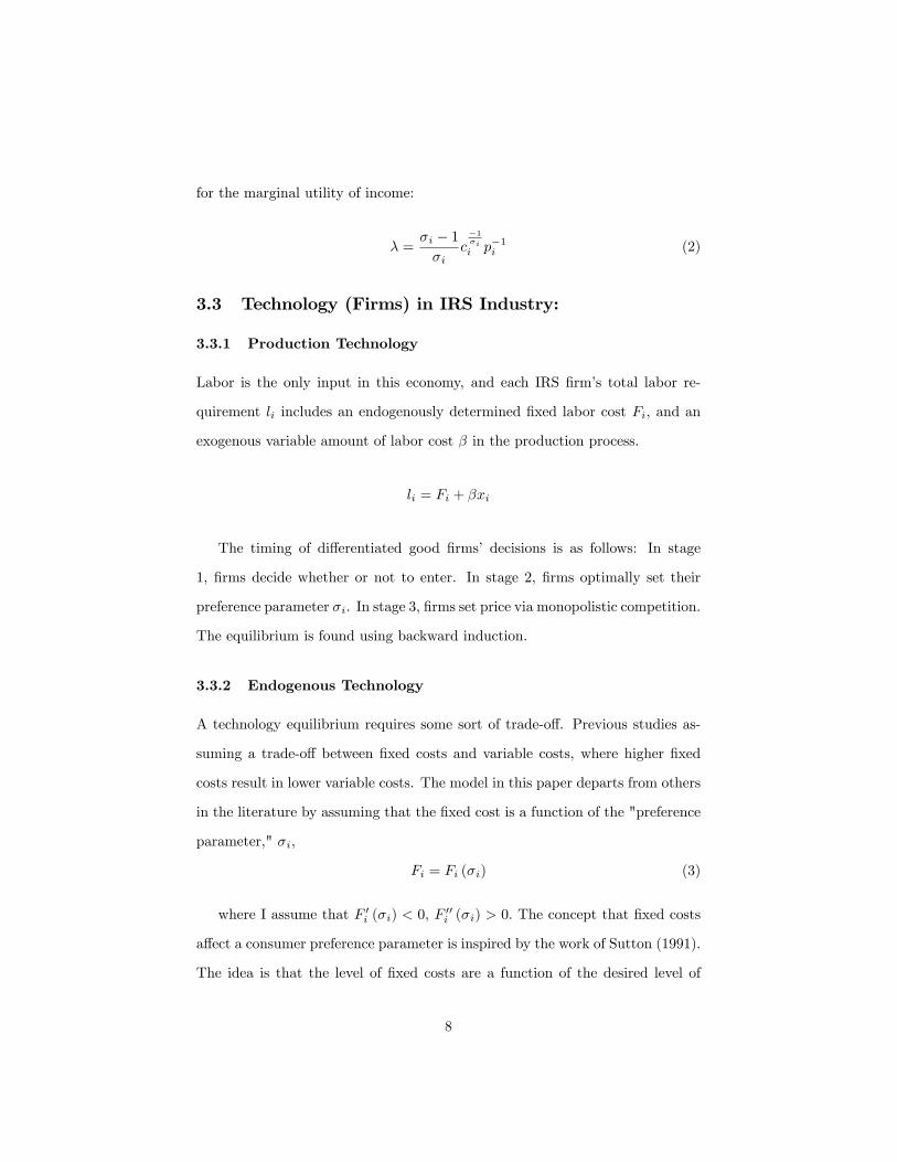
3.3 Technology (Firms) in IRS Industry:

3.3.1 Production Technology

Labor is the only input in this economy, and each IRS �rm�s total labor re-

quirement li includes an endogenously determined �xed labor cost Fi, and an

exogenous variable amount of labor cost � in the production process.

li = Fi + �xi

The timing of di¤erentiated good �rms� decisions is as follows: In stage

1, �rms decide whether or not to enter. In stage 2, �rms optimally set their

preference parameter �i. In stage 3, �rms set price via monopolistic competition.

The equilibrium is found using backward induction.

3.3.2 Endogenous Technology

A technology equilibrium requires some sort of trade-o¤. Previous studies as-

suming a trade-o¤ between �xed costs and variable costs, where higher �xed

costs result in lower variable costs. The model in this paper departs from others

in the literature by assuming that the �xed cost is a function of the "preference

parameter," �i,

Fi = Fi (�i) (3)

where I assume that F 0i (�i) < 0, F00i (�i) > 0: The concept that �xed costs

a¤ect a consumer preference parameter is inspired by the work of Sutton (1991).

The idea is that the level of �xed costs are a function of the desired level of

8

product di¤erentiation. Thus, di¤erentiating one�s own product from others (i.e.

lowering the preference parameter) would require higher �xed costs. These �xed

costs could be persuasive advertising or product development that di¤erentiates

a �rm�s own product from that of other �rms. I do not assume a functional

form at the moment, only that it is upward sloping and convex as �i decreases,

so that advertising expenditures exhibit decreasing returns. In addition, the

domain of the function must lie within (1;1), as this ensures that demand is

elastic. An example of a particular advertising function is given in �gure 1.

The notion that �xed costs can a¤ect consumer preferences is not novel.

Sutton�s (1991) partial equilibrium models endogenized �xed costs by assuming

that they augmented demand. Arkolakis (2006) also uses an advertising func-

tion, but it exhibits decreasing returns to reaching consumers. In contrast, this

paper�s advertising function exhibits decreasing returns to product di¤erentia-

tion. To the best of my knowledge, I cannot �nd any evidence in the literature

of modelling an explicit relationship between the elasticity of substitution and

�xed costs.

3.3.3 Stage 3: Setting price

In stage 3 the �rm sets price in order to maximize pro�t, and takes endogenous

�xed costs, Fi, as given from stage 2:

maxpi� = pixi � �xi � Fi

The �rst order condition is:

pi =�i

�i � 1�

9

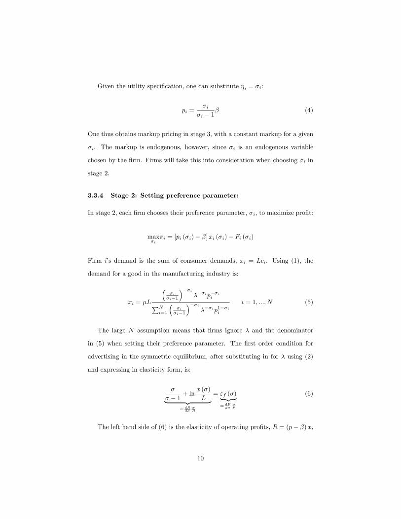
Given the utility speci�cation, one can substitute �i = �i:

pi =�i

�i � 1� (4)

One thus obtains markup pricing in stage 3, with a constant markup for a given

�i. The markup is endogenous, however, since �i is an endogenous variable

chosen by the �rm. Firms will take this into consideration when choosing �i in

stage 2.

3.3.4 Stage 2: Setting preference parameter:

In stage 2, each �rm chooses their preference parameter, �i, to maximize pro�t:

max�i�i = [pi (�i)� �]xi (�i)� Fi (�i)

Firm i�s demand is the sum of consumer demands, xi = Lci. Using (1), the

demand for a good in the manufacturing industry is:

xi = �L

��i�i�1

���i���ip��iiPN

i=1

��i�i�1

���i���ip1��ii

i = 1; :::; N (5)

The large N assumption means that �rms ignore � and the denominator

in (5) when setting their preference parameter. The �rst order condition for

advertising in the symmetric equilibrium, after substituting in for � using (2)

and expressing in elasticity form, is:

�

� � 1 + lnx (�)

L| {z }= dR

d��R

= "f (�)| {z }= dF

d��F

(6)

The left hand side of (6) is the elasticity of operating pro�ts, R = (p� �)x,

10

with respect to �. The right hand side of (6) is the elasticity �xed costs with

respect to �, denoted as "f (�). Note that (6) equates the marginal revenue and

marginal cost of increasing �, which explains why both sides of (6) are negative.

Given the assumptions about F (�), marginal cost increases and approaches

in�nity as � decreases to unity.

An illustration of the marginal revenue and marginal cost curves from (6)

is provided in �gure 1. Note that an isoelastic functional form of F (�) cannot

exist since it is assumed that F (�) approaches in�nity at � = 1. The advertising

function will thus have an elasticity that is negative and increasing in �, i.e.

@"f (�)@� > 0.

It can be shown that (6) is a maximum under fairly general conditions (see

Appendix A).

3.3.5 Stage 1: Entry decision

Firm entry occurs until pro�ts equal zero. Combining the pro�t maximization

condition and the zero pro�t condition, one obtains:

x =(� � 1)F (�)

�(7)

Inspection of (7) reveals that if the advertising function is F (�) = 1��1 then

x = ��1. The scale e¤ect is thus absent in this particular form of the advertising

function. However, F (�) can also be chosen such that x is an increasing or

decreasing function of �. In the latter case, this gives a positive scale e¤ect if

greater market size leads to a lower �. This is a useful property of this model,

since one can obtain scale e¤ects despite the CES utility speci�cation.

The full employment of labor condition nails down the number of �rms in

the manufacturing industry:

N =�L

F + �x(8)

11

Overall, equations (2), (3), (4), (6), (7) and (8) make up the autarky model.

This includes the same equations as a standard monopolistic competition model

for pro�t maximization in price, zero pro�ts, and full employment of labor, plus

(3) and (6). The unknowns are p, x, N , �, F , and �.

This system of equations is not analytically solvable without further assump-

tions about the shape of the advertising function. The problematic equation is

the �rst order condition for �. Nonetheless, one can show without any further

assumptions that � is decreasing in market size. In addition, the system can be

analytically solved for a special case of the advertising function, which is given

further on in the paper.

A simulation of the autarky model for di¤erent market sizes is given in

�gure 2. The simulation uses an advertising function with a positive scale e¤ect

(F (�) = 1(��1)2 ).

3.4 Market Size E¤ects

Substituting (2), (7) and (8) into (6) and using the implicit function theorem

to solve @�@L , provides the following condition:

@�

@L< 0, x0 (�)

x (�)<@"f (�)

@�| {z }>0

+ (� � 1)�2| {z }>0

Thus it can be shown that � decreases in market size under very general cir-

cumstances. This result means that goods become more di¤erentiated as the

market size increases.

The market size e¤ect on � a¤ects all of the other endogenous variables in

the model. As market size increases, �xed cost outlays will accordingly increase

via the relationship speci�ed in equation (3). Prices rise via the markup pricing

rule (4). As for the the market size e¤ect on variety, one can substitute (7) into

12

(8) to obtain a relationship between N and �:

N =�L

�F (�)(9)

Equation (9) illustrates that the the e¤ect of market size on variety depends

on how F and � vary with market size. In contrast to Krugman (1980), the

number of �rms need not increase linearly with market size. Likewise, the e¤ect

of market size on �rm scale also depends on the choice of advertising function,

as can be seen in (7).

The predictions of this model agree with respect to market size e¤ects agree

with the stylized facts as discussed by Mayer and Ottaviano (2007). Moreover, it

is generally accepted that �rm size increases with market size (Schmalansee 1989

p.992). I now move on to discuss a particular speci�cation of the advertising

function that simpli�es the analysis.

3.5 Solving the Autarky Model Fully

One problem with the model above is that an analytical solution cannot be ob-

tained without further assumptions about the shape of the advertising function.

This makes it di¢ cult to interpret equation (6), the �rst order condition for �.

However, one can fully solve the autarky model using the following advertising

function:

F (�) =1

� � 1 (10)

This form of the advertising is convex and downward sloping in �, and is as-

ymptotic to � = 1 (see �gure 1). This particular formulation has the special

property of having no "scale e¤ect", for reasons discussed below.

The �rst order and second order conditions using this particular advertising

13

function are:2�

� � 1 = ln�L

and�2

(� � 1)2< 0

In this case the lagrange multiplier, �, can be removed from the system of

equations and the analytical solution becomes:

p =ln�L

2�

x =1

�

N =2�L

ln�L

� =ln�L

ln�L� 2

F =ln�L

2� 1

This particular formulation of the advertising function is tractable because

it eliminates the problem of having a logged � term in the �rst order condition

for �. It does this by forcing x to equal 1� instead of the usual(��1)F (�)

� . This

means that there are no "scale e¤ects" (market size e¤ects on x) in this case.

Fixed costs and price are increasing and concave in � and L: Note also that

� is decreasing and convex in market size and marginal cost, and limL!1

� = 1.

Variety increases concavely with market size, which is an intuitive result if one

considers that N = �Lpx , where p increases concavely with market size. Any kind

of positive scale e¤ect would thus increase the concavity of variety growth.

Since the number of �rms increases without bound one can posit that limN!1

� =

1. This is the opposite conclusion of Lancaster�s (1979, 1980) "Ideal Variety"

14

approach to modelling monopolistic competition, where limN!1

� = +1. This re-

sult also contrasts with standard oligopoly theory, which generally asserts that

markups decrease as the number of �rms increase. The main reason for the

contradictory result of this paper is that product di¤erentiation is endogenous,

whereas other models of trade take product di¤erentiation as exogenous. The

endogeneity of product di¤erentiation expands the "product space" in the eyes

of consumers, so that competition becomes less tough despite the fact that more

�rms are entering the market. This is the intuition behind the market size result

that I obtain. One can obtain an analytical solution to the market size e¤ect

using the advertising function F (�) = 1��1 :

@�

@L=

�2L�1

(ln�L� 2)2< 0

3.6 A Closer Look at the Marginal Revenue Curve

The shape of the marginal revenue curve is di¢ cult to interpret from (6), but it is

illustrated in �gure 1. Inspection of �gure 1 reveals that the marginal revenue

curve is decreasing, then increasing, as � decreases. One can decompose the

marginal revenue function into a "markup e¤ect" and a "quantity e¤ect" in

order to understand this relationship. The operating pro�t of a �rm can be

given as:

R = (p� �)x

After log di¤erentiating and simplifying one obtains:

dR

R=

�� �

� � 1

�d�

�+

�lnx

L+ 2

�

� � 1

�d�

�(11)

The �rst term of (11) is the price e¤ect, which is always positive for decreases

in � and simply equal to the markup pricing rule. The second term is the

15

quantity e¤ect, which is either positive or negative for decreases in �, depending

on the sign of the term in the square brackets. One can see that ln xL is strictly

negative and 2 ���1 is strictly positive, and the relative size of these terms will

determine the sign of the quantity e¤ect. It is di¢ cult to say anything about the

this di¤erential since x and � are both endogenous. However, if one assumes that

the advertising function takes the functional form F (�) = 1��1 , then x =

1� ,

a constant, and one can see that decreasing marginal revenue occur can occur

whenever ���1 � ln (�L) > 0.

In sum, the price e¤ect on the marginal revenue from decreases in � is always

positive. The quantity e¤ect on marginal revenue is also positive when � is large,

but negative when � decreases. For low enough � the negative quantity e¤ect

outweighs the positive price e¤ect, which results in a marginal revenue curve

that is eventually downward sloping.

An alternative intuition is to recall that the quantity e¤ect is driven by the

term�

�i�i�1

��2�iin the numerator of equation (5), while the price e¤ect is

driven by�

�i�i�1

�1. The quantity e¤ect dominates as �i approaches unity.

4 Two Country Model

4.1 Setting, Preferences and Technology

Extending the autarky model to a two country model with iceberg trade costs

yields interesting results regarding the �rms�technology choice and the pattern

of trade. I begin by laying out the consumers�and �rms�optimization problems

and the relevant equations. I then interpret the e¤ect of market size and trade

liberalization on the endogenous variables.

The representative consumers at Home and Foreign solve the following util-

ity maximization problems:

16

maxUH = Nc��1�

H +N�c��

��1��

H s.t. NpcH +N��p�cH � �

maxUF = Nc��1�

F +N�c��

��1��

F s.t. N�pcF +N�p�cF � �

The H and F subscripts refer to Home and Foreign consumers respectively,

while the asterisk superscripts refer to the foreign �rm. Consumers are identical

in both countries and spend � of their income on di¤erentiated goods and 1��

of their income on a homogeneous agricultural good. When di¤erentiated goods

are shipped between countries, � units must be shipped in order for 1 unit to

arrive. Within a country, all �rms have identical sigmas, but they can di¤er

between countries.

The relevant equations of the two country model are given in Appendix B.

The two country model is not analytically solvable, but can be easily simulated.

4.2 Market Size E¤ects

Market size e¤ects in the two country model work in the same way as they do

in autarky, that is, � and �� are both decreasing in L and L�. Firms in the

country that face a greater market potential will have a lower sigma. If trade is

costly, this means that �rms in the larger country will produce goods that are

more di¤erentiated. This occurs since less of the world demand "melts away"

from the perspective of �rms in the larger country.

The model�s output under asymmetric country size is illustrated in �gure 3.

It follows from the asymmetric sigmas that �rms in di¤erent countries will have

asymmetric prices, �xed costs, and output per �rm as well. Namely, the larger

country will produce goods with higher markups, thus exporting higher priced

manufactured goods and importing lower priced manufactured goods. Fixed

costs will also be higher in the larger country, and output per �rm in the larger

17

country will be greater if the if the advertising function induces scale e¤ects, i.e.

@x(�)@� < 0. These predictions for prices and extensive margins are in accordance

with the results of Mayer and Ottaviano (2007). The result that the elasticity

of substitution is decreasing can also make some sense of Broda and Weinstein�s

(2006) result that the elasticity of substitution has been decreasing over time

despite the increase in "globalization" over the time of their sample.

If there are no trade costs, then �rms in both countries face the same market

potential and all the endogenous variables in both countries are identical.

4.3 Trade Cost E¤ects

The e¤ect of trade costs on the endogenous variables is an interesting aspect

of the model. It is illustrative to rearrange (24) under the special case where

country sizes are identical (i.e. L = L�):

"market size e¤ect"z }| {�

� � 1 + ln�

x (�)

L (1 + �1��)

��

"trade friction e¤ect"z }| {��1�� ln �

(1 + �1��)| {z }= dR

d��R

= "f (�)| {z }= dF

d��F

(12)

This equation e¤ectively divides the �rst order condition into two parts, a "mar-

ket size e¤ect" and a "trade friction e¤ect".

The "market size e¤ect" is almost identical to the left hand side of the

�rst order condition in autarky, (6), except for the additional term 1 + �1��

multiplying L in the denominator. This term equals 1 under in�nite trade costs

and 2 under free trade, since free trade between two countries of equal size

e¤ectively doubles the market.

The "trade friction e¤ect" is an additional term that is not present in the �rst

order condition under autarky. Note that�� �1�� ln �(1+�1��) =

�L(1+�1��)

@@�L

�1 + �1��

�,

which is the elasticity of market potential with respect to the elasticity of sub-

18

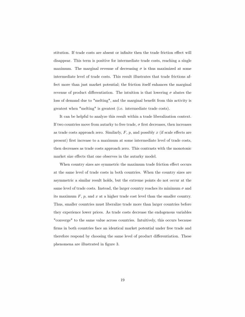
stitution. If trade costs are absent or in�nite then the trade friction e¤ect will

disappear. This term is positive for intermediate trade costs, reaching a single

maximum. The marginal revenue of decreasing � is thus maximized at some

intermediate level of trade costs. This result illustrates that trade frictions af-

fect more than just market potential; the friction itself enhances the marginal

revenue of product di¤erentiation. The intuition is that lowering � abates the

loss of demand due to "melting", and the marginal bene�t from this activity is

greatest when "melting" is greatest (i.e. intermediate trade costs).

It can be helpful to analyze this result within a trade liberalization context.

If two countries move from autarky to free trade, � �rst decreases, then increases

as trade costs approach zero. Similarly, F , p, and possibly x (if scale e¤ects are

present) �rst increase to a maximum at some intermediate level of trade costs,

then decreases as trade costs approach zero. This contrasts with the monotonic

market size e¤ects that one observes in the autarky model.

When country sizes are symmetric the maximum trade friction e¤ect occurs

at the same level of trade costs in both countries. When the country sizes are

asymmetric a similar result holds, but the extreme points do not occur at the

same level of trade costs. Instead, the larger country reaches its minimum � and

its maximum F , p, and x at a higher trade cost level than the smaller country.

Thus, smaller countries must liberalize trade more than larger countries before

they experience lower prices. As trade costs decrease the endogenous variables

"converge" to the same value across countries. Intuitively, this occurs because

�rms in both countries face an identical market potential under free trade and

therefore respond by choosing the same level of product di¤erentiation. These

phenomena are illustrated in �gure 3.

19

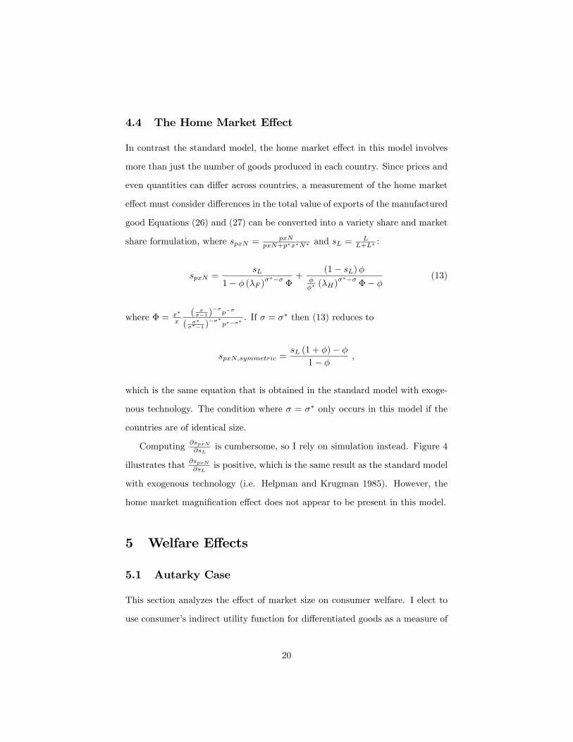
4.4 The Home Market E¤ect

In contrast the standard model, the home market e¤ect in this model involves

more than just the number of goods produced in each country. Since prices and

even quantities can di¤er across countries, a measurement of the home market

e¤ect must consider di¤erences in the total value of exports of the manufactured

good Equations (26) and (27) can be converted into a variety share and market

share formulation, where spxN =pxN

pxN+p�x�N� and sL = LL+L� :

spxN =sL

1� � (�F )����

�+

(1� sL)���� (�H)

������ �

(13)

where � = x�

x

( ���1 )

��p��

( �����1 )

���p����

. If � = �� then (13) reduces to

spxN;symmetric =sL (1 + �)� �

1� � ,

which is the same equation that is obtained in the standard model with exoge-

nous technology. The condition where � = �� only occurs in this model if the

countries are of identical size.

Computing @spxN@sL

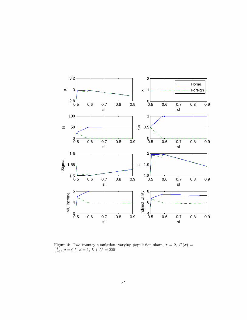
is cumbersome, so I rely on simulation instead. Figure 4

illustrates that @spxN@sLis positive, which is the same result as the standard model

with exogenous technology (i.e. Helpman and Krugman 1985). However, the

home market magni�cation e¤ect does not appear to be present in this model.

5 Welfare E¤ects

5.1 Autarky Case

This section analyzes the e¤ect of market size on consumer welfare. I elect to

use consumer�s indirect utility function for di¤erentiated goods as a measure of

20

welfare. In autarky, the indirect utility function is clearly increasing in variety

and decreasing in price. The e¤ect of � on indirect utility, however, is unclear:

� = N1�

��

p

���1�

The e¤ect of market size on consumer welfare is thus not straight forward,

since variety increases but the real wage decreases as the market expands. This

contrasts with the standard model that assumes exogenous technology, where

the real wage is constant and welfare e¤ects occur exclusively via increased

variety.

One can express the indirect utility function in terms of only L and �:

� (L; �) = �L1� [�F (�)]

� 1�

�� � 1�

���1�

The total di¤erential of indirect utility with respect to market size is:

d�

dL=@�

@L+@�

@�

@�

@L

The direct e¤ect, @�@L , is positive because of the increase in the number of vari-

eties, but the indirect e¤ect is requires further calculation. It has already been

shown that @�@L is negative under fairly general conditions, so the e¤ect of market

size on utility depends on @�@� :

@�

@�= N

1�

�� � 1�

���1� 1

�2

�ln�x

L� �F

0 (�)

F (�)

�

The condition for a negative sign on the derivative is:

@�

@�< 0, ln

�x

L� �F

0 (�)

F (�)< 0 (14)

21

It is not clear (14) holds, but if one assumes that the advertising function

takes the form F (�) = 1��1 then the condition for a negative sign on the deriv-

ative is:@�

@�< 0, ln� < lnL

This inequality will hold, which illustrates that market size has an unambigu-

ously positive impact on utility in this case. Indeed, for any advertising function

where (14) holds, market size positively a¤ects consumer utility. Thus the pos-

itive "product di¤erentiation" e¤ect outweighs the negative real wage e¤ect.

The autarky simulation in �gure 2 reveals that indirect utility is monotonically

increasing in market size for an advertising function with positive scale e¤ects.

5.2 Two Country Case - Welfare E¤ects

5.2.1 Welfare E¤ect of Market Size

The e¤ect of changing market size or changing trade costs is not straight forward.

However, it can be shown that larger markets experience greater utility, since

the variety e¤ect and the product di¤erentiation e¤ect dominate the real wage

e¤ect under fairly general conditions. Figure 4 illustrates that indirect utility is

an increasing function of population share.

5.2.2 Welfare E¤ect of Trade Costs

The total di¤erential of indirect utility with respect to market size is:

d�

d�=@�

@�+@�

@�

@�

@�

22

Derivation of indirect utility with respect to � reveals that the direct e¤ect is

clearly negative:

@

@�� (L; � ; �) = �L

1� [�F (�)]

� 1�

�� � 1�

���1� 1

�

�1 + �1��

� 1��1 (1� �) ��� < 0

(15)

The indirect e¤ect, @�@�@�@� , is more di¢ cult to ascertain. It was shown in the

previous section that @�@� will be negative under fairly general circumstances.

The problematic derivative is @�@� , since (15) illustrates that

@�@� is negative for

lower trade costs and positive for higher trade costs, which makes prediction of

the sign di¢ cult. However, one can say that higher trade costs unequivocally

result in lower utility when trade costs are high enough.

Figure 3 illustrates using a numerical simulation that indirect utility is

monotonically increasing as trade costs decrease. Once again the positive variety

di¤erentiation e¤ect outweighs the negative real wage e¤ect.

5.3 Market Equilibrium versus Optimum

It can be useful to compare the market equilibrium with the constrainted and

unconstrained optimum, and also to compare to the results of the standard

Dixit-Stiglitz model of monopolistic competition. The market equilibrium in

autarky has already been described above, and di¤ers from Krugman (1980) by

pinning down the level of �xed costs and the elasticity of substitution.

The constrained optimum maximizes utility subject to �rms breaking even.

The constrained optimum in this paper di¤ers from the standard result by also

pinning down the level of �xed costs and the elasticity of substitution. The �rst

order condition for the elasticity of subsitution in the constrained case is

ln1

�+ lnx = "f ,

23

where "f is the elasticity of �xed costs with respect to the elasticity of subsitution

This is very similar to the market equilibrium �rst order condition (6). The

most notable di¤erence is that market size does not matter in the constrained

optimum. Assuming F = 1��1 , one can clearly see the condition for the market

equilibrium to be more di¤erentiated (i.e. lower �) than constrained optimal:

ln1

�>

�

� � 1 � lnL

Thus, the market equilibrium does not di¤erentiate products enough in small

markets, while it results in more than optimal product di¤erentiation in large

markets.

6 Testing the Model

This model predicts that �xed costs, markups, and output per �rm are in-

creasing functions of market size, and are maximized at some intermediate level

of trade costs. Furthermore, the impact of trade liberalization on �xed costs,

markups, and output per �rm is more pronounced for smaller countries. These

hypotheses may be empirically testable.

The most unique property of this model is the trade friction e¤ect. A test of

the model would be to derive a gravity model for prices. Mayer and Ottaviano

(2007) estimated a gravity equation for prices with monotonic distance and

market size e¤ects. In this case, the gravity equation would have to allow

for the non-monotonic trade friction e¤ect to be evaluated. If such a gravity

model revealed that prices are highest at intermediate trade costs, this would

be compelling evidence for the existence of the trade friction e¤ect.

24

7 Conclusion

The model presented in the paper takes a new look at product di¤erentiation in

the Dixit-Stiglitz model of monopolistic competition. Moreover, it has several

attractive features that agree with the stylized facts on trade. First, the model

allows for �rms to endogenously choose from a continuous set of technologies by

creating a trade-o¤ between �xed costs and the elasticity of substitution. This

is an appropriate assumption if �xed costs represent persuasive advertising or

product development that di¤erentiate one�s own product from others in the

eyes of consumers. To the best of my knowledge, the idea of endogenizing the

elasticity of substitution in order to endogenize technology is novel. Second,

the model allows for scale e¤ects, despite having CES utility properties in the

symmetric equilibrium. Third, �xed costs, markups, and output per �rm are

increasing functions of market size, a characteristic that agrees with the liter-

ature. Fourth, the model produces "endogenous markups" that are a direct

result of �rms�optimizing behavior.

The result that markups increase with market size may be considered some-

what controversial, since the "conventional wisdom" is that markups will de-

crease as market size increases, �rms enter, and the competition becomes "tougher."

This model o¤ers an alternative explanation when product di¤erentiation is en-

dogenous and works via the elasticity of substitution parameter. As Tirole

(1988, p.289) puts it, "Though it will be argued that advertising may foster

competition by increasing the elasticity of demand (reducing "di¤erentiation"),

it is easy to �nd cases in which the reverse is true." It is hoped that this paper

has given some theoretical foundation to this argument.

25

Appendix AThe second order condition is:

@2�

@�2< 0, x0 (�)

x (�)<@"f (�)

@�| {z }>0

+ (� � 1)�2| {z }>0

The second order condition is met as for any advertising function that exhibits

non-negative scale e¤ects (i.e. x0 (�) � 0). This condition can also be met if

x0 (�) > 0 as long as the inequality holds (i.e. as long as the scale e¤ect is not

too strong).

Appendix BThe marginal utilities of income for Home consumers can be expressed in

two ways:

�H =� � 1�

c�1�

H p�1

�H =�� � 1��

c��1��

H ��1p��1

The demand for a Home �rm�s good is:

x = LcH + �L�cF (16)

= �L

����1

������H p��

N�

���1

������H p1�� +N�

���

���1

�������

�

H p�1�����

+�L�

����1

������F p���

N�

���1

������F p1���+N�

���

���1

�������

�

F p�1���

26

and the demand for a Foreign �rm�s good is:

x� = �Lc�H + L�c�F (17)

= �L

���

���1

�������

�

H p������

N�

���1

������H p1�� +N�

���

���1

�������

�

H p�1�����

+�L�

���

���1

�������

�

F p����

N�

���1

������F p1���+N�

���

���1

�������

�

F p�1���

where � = �1�� and �� = �1���.

As in the autarky model, �rms set price in the last stage. The �rst order

conditions for p and p� are:

p =�

� � 1� (18)

p� =��

�� � 1� (19)

The zero pro�t conditions at Home and Foreign can be written as:

x =(� � 1)F (�)

�(20)

and

x� =(�� � 1)F (��)

�(21)

Home and Foreign �rms choose the optimum level of �, ��, F and F � in stage

2. The advertising functions for Home and Foreign �rms are:

F = F (�) (22)

F � = F (��) (23)

Firms in both countries thus abide by the same advertising function, but the

27

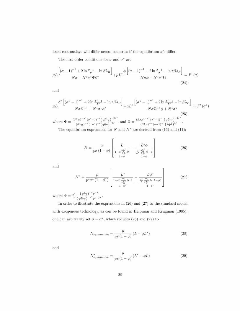
�xed cost outlays will di¤er across countries if the equilibrium ��s di¤er.

The �rst order conditions for � and �� are:

�L

h(� � 1)�1 + 2 ln ��1� � ln��H

iN� +N�����

+�L��h(� � 1)�1 + 2 ln ��1� � ln ���F

iN��+N���

= F 0 (�)

(24)

and

�L��h(�� � 1)�1 + 2 ln ���1�� � ln ���H

iN��1 +N�����

+�L�

h(�� � 1)�1 + 2 ln ���1�� � ln��F

iN��1�+N���

= F 0 (��)

(25)

where =(��H)

��� (���1)�1( �����1 )

�2��

(��H)��(��1)�1( �

��1 )�2� and =

(��F )��� (���1)�1( ��

���1 )�2��

(��F )��(��1)�1(��1� )

2� .

The equilibrium expressions for N and N� are derived from (16) and (17):

N =�

px (1� �)

2664 L

1�����

F��F�

1��

� L��

���

���

H��H���

1��

3775 (26)

and

N� =�

p�x� (1� ��)

2664 L�

1��� ��H

���

H

��1

1���

� L��

���

��F

���

F

��1���

1���

3775 (27)

where � = x�

x

( ���1 )

��p��

( �����1 )

���p����

.

In order to illustrate the expressions in (26) and (27) to the standard model

with exogenous technology, as can be found in Helpman and Krugman (1985),

one can arbitrarily set � = ��, which reduces (26) and (27) to

Nsymmetric =�

px (1� �) (L� �L�) (28)

and

N�symmetric =

�

px (1� �) (L� � �L) (29)

28

Equations (28) and (29) are identical to those of the standard model with ex-

ogenous technology. The condition where � = �� only occurs in this model if

the countries are of identical size. One crucial di¤erence between (26) and (27)

and the standard Helpman and Krugman expressions is that px and p�x� will

increase as the market expands in (26) and (27), which negatively a¤ects variety.

On the other hand, L and L� are divided by terms in the square brackets that

will change as the market expands.

Overall, equations (18) through (27) make up the two country model.

29

References

Akerman, A. and R. Forslid (2007). Country Size, Productivity and TradeShare Convergence: An Analysis of Heterogenous Firms and Country SizeDependent Beachhead Costs. CEPR Discussion Paper 6545.

Arkolakis, C. (2006). Market Access Costs and the New Consumers Margin inInternational Trade. Unpublished manuscript, University of Minnesota.

Broda, C. and D.E. Weinstein (2006). Globalization and the Gains from Vari-ety. American Economic Review 121(2), 541-585.

Bustos, P. (2005). Rising Wage Inequality in the Argentinean ManufacturingSector: The Impact of Trade and Foreign Investment on Technology andSkill Upgrading. unpublished manuscript, Harvard University.

Butters, G. (1977). Equilibrium Distributions of Sales and Advertising Prices.Review of Economic Studies, 44, 465-491.

Dinopolous, E. and P. Segerstrom (1999). A Shumpetarian model of Protectionand Relative Wages. American Economic Review 89, 450-472.

Dixit, A. K. and J. E. Stiglitz (1977). Monopolistic Competition and OptimumProduct Diversity. American Economic Review 67, 297�308.

Elberfeld, W. and G. Götz (2002), Market Size, Technology Choice, and MarketStructure. German Economic Review 3, 25�41.

Eckel, C. (2006). Trade and Diversity: Is there a Case for �Cultural Protec-tionism?�, German Economic Review 7, 403-418.

Ekholm, K., Midelfart Knarvik, K., 2005. Relative Wages and Trade-InducedChanges in Technology. European Economic Review 49, 1637-1663.

Feenstra, R. (1994). New Product Varieties and the Measurement of Interna-tional Prices. American Economic Review 84(1), 157-177.

Grossman, G. M. and E. Helpman. Innovation and growth in the global econ-omy. MIT Press, Cambridge, MA.

Krugman, P. (1979). Increasing Returns, Monopolistic Competition, and In-ternational Trade. Journal of International Economics 9, 469-479.

Krugman, P. (1980). Scale Economies, Product Di¤erentiation, and the Pat-tern of Trade. American Economic Review 70, 950�959.

Lancaster, K. (1979). Variety, Equity, and E¢ ciency. Basil Blackwell, Oxford.

Lancaster, K. (1980). Competition and Product Variety. Journal of Business53, 79�103.

30

Markusen, J. and A. J. Venables (1997). The Role of Multinational Firms inthe Wage Gap Debate. Review of International Economics 5, 435-451.

Mayer, T. and G. Ottaviano (2007). The Happy Few: The internationisation ofEuropean �rms: New facts based on �rm-level evidence. Bruegel BlueprintSeries Volume III. Bruegel/CEPR, Brussels.

Melitz, M. (2003). The Impact of Trade on Intra-Industry Reallocations andAggregate Industry Productivity. Econometrica 71, 1695-1725.

Melitz, M. and G. Ottaviano (2005). Market Size, Trade and Productivity.NBER working paper 11393.

Neary, J.P. (2002). Foreign competition and wage inequality. Review of Inter-national Economics, 10(4), 680-693.

Neary, J.P. (2003), Globalization and market structure. Journal of the Euro-pean Economic Association 1, 245-271.

Ottaviano, G., T. Tabuchi and J.F. Thisse (2002). Agglomeration and TradeRevisited. International Economic Review 43(2), 409-435.

Ravenga, A. (1997). Employment and Wage E¤ects of Trade Liberalization:The Case of Mexican Manufacturing. Journal of Labor Economics 15(3),20-43.

Schmalensee, R., 1989. Inter-industry studies of structure and performance.In: Schmalensee, R., Willig, R.D. (Eds.). Handbook of Industrial Orga-nization, Vol. II. North-Holland, Amsterdam, pp. 951�1009.

Schott, P. K., 2004. Across-Product versus Within-Product Specialization inInternational Trade. Quarterly Journal of Economics 119(2): 647-678.

Sutton, J. (1991). Sunk Costs and Market Structure. MIT Press, Cambridge,MA.

Tirole, J. (1988). The Theory of Industrial Organization. MIT Press, Cam-bridge, MA.

Tre�er, D. (2004). The Long and Short of the Canada-U.S. Free Trade Agree-ment. American Economic Review 94(4), 870-895.

Yeaple, S.R. (2005). A Simple Model of Firm Heterogeneity, InternationalTrade, and Wages. Journal of International Economics 65, 1-20.

31

Figure 1: Advertising, Marginal Revenue and Marginal Cost Curves, F (�) =1

1�� , L = 100, � = 1

32

0 500 1000 1500 20001.5

2

2.5

Market Size

p

0 500 1000 1500 20000.5

1

1.5

Market Size

x0 500 1000 1500 2000

0

200

400

Market Size

N

0 500 1000 1500 20001

2

3

Market Size

Sig

ma

0 500 1000 1500 20000

2

4

Market Size

F

0 500 1000 1500 20000

10

20

Market size

MU

 inco

me

0 500 1000 1500 20000

10

20

Market size

Indi

rect

 Util

ity

Figure 2: Autarky simulation, F (�) = 1(��1)2 , � = 0:5, � = 1

33

0 5 102.6

2.8

3

tao

p

0 5 100

1

2

tao

x

HomeForeign

0 5 100

50

tao

N

0 5 100

0.5

1

tao

Sn

0 5 101.5

1.6

1.7

tao

Sig

ma

0 5 101.6

1.8

2

tao

F

0 5 102

4

6

tao

MU

 inco

me

0 5 104

5

6

tao

Indi

rect

 Util

ity

Figure 3: Two country simulation, varying trade costs, L = 120, L� = 100,F (�) = 1

��1 , � = 0:5, � = 1

34

0.5 0.6 0.7 0.8 0.92.8

3

3.2

sl

p

0.5 0.6 0.7 0.8 0.90

1

2

sl

x

HomeForeign

0.5 0.6 0.7 0.8 0.90

50

100

sl

N

0.5 0.6 0.7 0.8 0.90

0.5

1

sl

Sn

0.5 0.6 0.7 0.8 0.91.5

1.55

1.6

sl

Sig

ma

0.5 0.6 0.7 0.8 0.91.8

1.9

2

sl

F

0.5 0.6 0.7 0.8 0.93

4

5

sl

MU

 inco

me

0.5 0.6 0.7 0.8 0.94

6

8

sl

Indi

rect

 Util

ity

Figure 4: Two country simulation, varying population share, � = 2, F (�) =1

��1 , � = 0:5, � = 1, L+ L� = 220

35