
A Model of Capital and Crises - mfm.uchicago.edu
44
A Model of Capital and Crises Zhiguo He and Arvind Krishnamurthy November 2011
Transcript of A Model of Capital and Crises - mfm.uchicago.edu

A Model of Capital and CrisesZhiguo He and Arvind KrishnamurthyNovember 2011

“rdr036” — 2011/11/11 — 17:41 — page 1 — #1
Review of Economic Studies (2011)xx, 1–43 doi: 10.1093/restud/rdr036 The Author 2011. Published by Oxford University Press on behalf ofThe Review of Economic Studies Limited.
A Model of Capital and CrisesZHIGUOHE
BoothSchool of Business, University of Chicago
and
ARVINDKRISHNAMURTHY
Kellogg School of Management, Northwestern University and NBER
First version received December2008; final version accepted May2011 (Eds.)
We develop a model in which the capital of the intermediary sector plays a critical role in deter-mining asset prices. The model is cast within a dynamic general equilibrium economy, and the role forintermediation is derived endogenously based on optimal contracting considerations. Low intermediarycapital reduces the risk-bearing capacity of the marginal investor. We show how this force helps to explainpatterns during financial crises. The model replicates the observed rise during crises in Sharpe ratios, con-ditional volatility, correlation in price movements of assets held by the intermediary sector, and fall inriskless interest rates.
Key words: Liquidity, Hedge funds, Delegation, Financial institutions
JEL Codes: G12, G2, E44
1. INTRODUCTION
Financial crises, such as the hedge fund crisis of 1998 or the 2007/2008 subprime crisis, haveseveral common characteristics: risk premia rise, interest rates fall, conditional volatilities ofasset prices rise, correlations between assets rise, and investors “fly to the quality” of a risklessliquid bond. This paper offers an account of a financial crisis in which intermediaries play thecentral role. Intermediaries are the marginal investors in our model. The crisis occurs becauseshocks to the capital of intermediaries reduce their risk-bearing capacity, leading to a dynamicthat replicates each of the aforementioned regularities.
Our model builds on the liquidity models common in the banking literature (see in particular,Allen and Gale, 1994;Holmstrom and Tirole,1997). There are two classes of agents, householdsand specialists. The specialists have the know-how to invest in a risky asset, which the house-holds cannot directly invest in. This leads to the possibility of gains from trade. The specialistsaccept moneys from the households and invest in the risky asset on the households’ behalf. Interms of the banking models, we can think of the specialist as the manager of a financial in-termediary that raises financing from the households. However, this intermediation relationshipis subject to a moral hazard problem. Agents choose a financial contract to alleviate the moralhazard problem. The financial contract features anequity capital constraint: if the specialistmanaging an intermediary has wealthWt , the household will provide at mostmWt of equity fi-nancing to the intermediary. Here,m is a function of the primitives of the moral hazard problem.
There are many models in the banking literature that study intermediation relationshipssubject to financial constraints. However, most of the literature considers one- or two-period
1
The Review of Economic Studies Advance Access published November 17, 2011 at Serials D
epartment on January 11, 2012
http://restud.oxfordjournals.org/D
ownloaded from

“rdr036” — 2011/11/11 — 17:41 — page 2 — #2
2 REVIEW OF ECONOMIC STUDIES
equilibrium settings (the typical model is a “t = 0,1,2” model). We embed this intermediationstage game in an infinite-horizon setting. That is, the households and specialists interact at datet to form an intermediary, as described above, and make financing and asset trading decisions.Shocks realize and lead to changes in the wealth levels of both specialists and households, as afunction of the intermediation relationship formed at datet . Then in the next period, given thesenew wealth levels, intermediation relationships are formed again, and so on so forth.
The advantage of the infinite-horizon setting is that it is closer to the models common in theasset pricing literature and can thus more clearly speak to asset pricing phenomena in a crisis.The asset market is modelled along the lines ofLucas(1978). There is a risky asset producingan exogenous but risky dividend stream. The specialists can invest in the risky asset directly butthe household cannot. There is also a riskless bond in which all agents can invest. We use ourmodel to compute a number of asset pricing measures, including the risk premium, interest rate,and conditional volatility, and relate these measures to intermediary capital.1
Mostof our model’s results can be understood by focusing on the dynamics of the equity cap-ital constraint. Consider a given state described by the specialists’ wealthWt andthe households’wealthWh
t . The capital constraint requires that the household can invest at mostmWt (whichmaybe less thanWh
t ) in intermediaries as outside equity capital. Thus, intermediaries have totalcapital of at mostWt + mWt to purchase the risky asset. In some states of the world, this totalcapital is sufficient that the risk premium is identical to what would arise in an economy withoutthe capital constraint. This corresponds to the states whereWt is high and the capital constraintis slack. Now imagine loweringWt . There is a critical point at which the capital constraint willbegin to bind and affect equilibrium. In this case, the total capital of the intermediary sector islow. However, in general equilibrium, the low total intermediary capital must still go towardspurchasing the total supply of the risky asset, which in equilibrium results in market prices ad-justing. More specifically, the limited intermediary capital bears a disproportionate amount ofasset risk, and to clear the asset market, the risk premium rises. Moreover, from this state, if thedividend on the risky asset falls,Wt falls further, causing the capital constraint to bind further,thereby amplifying the negative shock. This amplification effect produces the rise in volatilitywhen intermediary capital is low. Finally, fallingWt induceshouseholds to reallocate their fundsfrom the intermediary sector towards the riskless asset. The increased demand for bonds causesthe interest rate to fall. As noted above, each of these results match empirical observations duringliquidity crises.2
Thepaper is related to a large literature in banking studying disintermediation and crises (seeAllen and Gale, 1994;Holmstrom and Tirole, 1997;Diamond and Rajan, 2005). We differ fromthis literature in that our model is dynamic, while much of this literature is static.Brunnermeierand Sannikov(2010) is another recent paper that develops a model that is fully dynamic andlinks intermediaries’ financing position to asset prices. Our paper is also related to the literatureon limits to arbitrage studying how impediments to arbitrageurs’ trading strategies may affect
1. In a companion paper (He and Krishnamurthy,2010), we develop these points further by incorporating addi-tional realistic features into the model so that it can be calibrated. We show that the calibrated model can quantitativelymatch crisis asset market behaviour.
2. The dynamics of the capital constraint in our model parallels results in the recent long-term contracting lit-erature (e.g.DeMarzo and Sannikov, 2006;Biais et al., 2007;DeMarzo and Fishman, 2007). In these models, aftera sequence of poor performance realizations, the long-term contract punishes the agent and leaves the agent with lowcontinuation utility or a low “inside” stake in the project. Then, because of limited liability, the principal finds it harderto provide incentives for the agent to exert effort, resulting in a more severe agency friction. In our model, we restrictattention to short-term contracts. Nevertheless, our model’s results have this dynamic flavour: negative shocks result inlow specialist wealth, which tightens the incentive constraint and exacerbates the agency frictions in the intermediationrelationship between household and specialist.
at Serials Departm
ent on January 11, 2012http://restud.oxfordjournals.org/
Dow
nloaded from

“rdr036” — 2011/11/11 — 17:41 — page 3 — #3
HE & KRISHNAMURTHY A MODEL OF CAPITAL AND CRISES 3
equilibrium asset prices (Shleifer and Vishney, 1997). One part of this literature explores theeffects of margin or debt constraints for asset prices and liquidity in dynamic models (seeGromband Vayanos, 2002;Brunnermeier and Pedersen,2008;Geanakoplos and Fostel, 2008; Adrianand Shin, 2010). Our paper shares many objectives and features of these models. The principaldifference is that we study a constraint on raising equity capital, while these papers study aconstraint on raising debt financing.Xiong (2001) andKyle and Xiong(2001) model the effectof arbitrageur capital on asset prices by studying an arbitrageur with log preferences, where riskaversion decreases with wealth. The effects that arise in our model of equity capital constraintsare qualitatively similar to these papers. An advantage of our paper is that intermediaries andtheir equity capital are explicitly modelled allowing our paper to better articulate the role ofintermediaries in crises.3 Vayanos(2005) also more explicitly models intermediation. His modelalso explains the increase in conditional volatility during crises. However, his approach is tomodel an open-ending friction, rather than a capital friction, into a model of intermediation.Finally, many of our asset pricing results come from assuming that some markets are segmentedand that households can only trade in these markets by accessing intermediaries. Our paper isrelated to the literature on asset pricing with segmented markets (seeAllen and Gale, 1994;Alvarez, Atkeson and Kehoe, 2002;Edmond and Weill,2009).4
Empirically, the evidence for an intermediation capital effect comes in two forms. First, bynow it is widely accepted that the fall of 1998 crisis was due to negative shocks to the capitalof intermediaries (hedge funds, market makers, trading desks, etc.). These shocks led interme-diaries to liquidate positions, which lowered asset prices, further weakening intermediary bal-ance sheets.5 Similarcapital-related phenomena have been noted in the 1987 stock-market crash(Mitchell, Pederson and Pulvino, 2007), the mortgage-backed securities market following anunexpected prepayment wave in 1994 (Gabaix, Krishnamurthy and Vigneron,2007), as well thecorporate bond market following the Enron default (Berndtet al., 2004).Froot and O’Connell(1999) andFroot (2001) present evidence that the insurance cycle in the catastrophe insurancemarket is due to fluctuations in the capital of reinsurers.Duffie (2010) discusses some of thesecases in the context of search costs and slow movement of capital into the affected intermediatedmarkets.Duffie and Strulovici(2011) present a search-based model of the slow movement ofcapital. One of the motivations for our paper is to reproduce asset market behaviour during crisisepisodes.
Although the crisis evidence is dramatic, crisis episodes are rare and do not lend themselvesto systematic study. The second form of evidence for the existence of intermediation capitaleffects comes from studies examining the cross-sectional/time-series behaviour of asset priceswithin a particular asset market.Gabaix, Krishnamurthy and Vigneron(2007) study a cross-section of prices in the mortgage-backed securities market and present evidence that the marginalinvestor who prices these assets is a specialized intermediary rather than a Capital Asset PricingModel-type representative investor. Similar evidence has been provided for index options (Bates,2003;Garleanu, Pederson and Poteshman, 2009) and corporate bonds and default swaps (Collin-Dufresne, Goldstein and Martin, 2001; Berndt et al., 2004). Adrian, Etula and Muir(2011)
3. The same distinction exists between our paper andPavlova and Rigobon(2008), who study a model with log-utility agents facing exogenous portfolio constraints and use the model to explore some regularities in exchange ratesand international financial crises. Like us, their model shows how contagion and amplification can arise endogenously.While their application to international financial crises differs from our model, at a deeper level the models are related.
4. Our model is also related to the asset pricing literature with heterogenous agents (seeDumas,1989;Wang,1996;Longstaff and Wang, 2008).
5. Other important asset markets, such as the equity or housing market, were relatively unaffected by the turmoil.The dichotomous behaviour of asset markets suggests that the problem was hedge fund capital specifically and notcapital more generally.
at Serials Departm
ent on January 11, 2012http://restud.oxfordjournals.org/
Dow
nloaded from

“rdr036” — 2011/11/11 — 17:41 — page 4 — #4
4 REVIEW OF ECONOMIC STUDIES
offer empirical evidence that a single factor constructed from the leverage of the intermediarysector can successfully price the size, book-to-market, as well as momentum and industry stockportfolios. These studies reiterate the relevance of intermediation capital for asset prices.
This paper is laid out as follows. Section2 describes the model and derives the capitalconstraint based on agency considerations. Section3 describes the intermediation market andagent’s decisions. Section4 solves for asset prices in closed form and studies the implicationsof intermediation capital on asset pricing. Section5 discusses the contracting issues that arise inour model in further detail. Section6 explains the parameter choices in our numerical examples,and Section7 concludes. We place most proofs in the Appendix that follows.
2. THE MODEL
2.1. Agents and assets
We consider an infinite-horizon continuous-time economy with a single perishable consumptiongood, along the lines ofLucas(1978). We use the consumption good as the numeraire. Thereare two assets, a riskless bond in zero net supply and a risky asset that pays a risky dividend. Wenormalize the supply of the risky asset to be one unit.
The risky asset pays a dividend ofDt per unit of time, where{Dt : 0 ≤ t < ∞} follows ageometric Brownian motion,
d Dt
Dt= gdt +σd Zt given D0, (1)
whereg > 0 andσ > 0 are constants. Throughout this paper,{Z} = {Zt : 0 ≤ t < ∞} is a stan-dard Brownian motion on a complete probability space(�,F ,P) with an augmented filtration{Ft : 0 ≤ t < ∞} generated by the Brownian motion{Z}.
We denote the progressively measurable processes{Pt : 0 ≤ t < ∞} and{rt : 0 ≤ t < ∞} asthe risky asset price and interest rate processes to be determined in equilibrium. We write thetotal return on the risky asset as
d Rt =Dtdt +d Pt
Pt= μR,t dt +σR,t dZt , (2)
whereμR,t is the risky asset’s expected return andσR,t is the volatility. The risky asset’s riskpremiumπR,t is
πR,t ≡ μR,t − rt .
Thereare two classes of agents in the economy, households and specialists. Without lossof generality, we set the measure of each agent class to be one. We are interested in studyingan intermediation relationship between households and specialists. To this end, we assume thatthe risky asset pay-off comprises a set of complex investment strategies (e.g.mortgage-backedsecurities investments) that the specialist has a comparative advantage in managing and thereforeintermediates the households’ investments in the risky asset.
As in the literature on limited market participation (e.g.Mankiw and Zeldes,1991;Allen andGale,1994;Basak and Cuoco, 1998;Vissing-Jorgensen, 2002), we make the extreme assumptionthat the household cannot directly invest in the risky asset and can directly invest only in thebond market. We motivate this assumption by appealing to “informational” transaction coststhat households face in order to invest directly in the risky asset market.
We depart from the limited participation literature by allowing specialists to invest in therisky asset on behalf of the households. However, there is a moral hazard problem that affectsthis intermediation relationship. Households write an optimally chosen financial contract with
at Serials Departm
ent on January 11, 2012http://restud.oxfordjournals.org/
Dow
nloaded from

“rdr036” — 2011/11/11 — 17:41 — page 5 — #5
HE & KRISHNAMURTHY A MODEL OF CAPITAL AND CRISES 5
FIGURE 1The economy
the specialist to alleviate the moral hazard problem. Figure1 provides a graphical representationof our economy.
Both specialists and households are infinitely lived and have log preferences over datetconsumption. Denotect (ch
t ) as the specialist’s (household’s) consumption rate. The specialistmaximizes
E[∫ ∞
0e−ρt lnctdt
],
while the household maximizes
E[∫ ∞
0e−ρht lnch
t dt
],
where the positive constantsρ andρh are the specialist’s and household’s time-discount rates,respectively. Throughout, we use the superscript “h” to indicate households. Note thatρ maydiffer from ρh; this flexibility is useful when specifying the boundary condition for the economy.
2.2. Intermediaries and intermediation contract
At every t , households invest in intermediaries that are run by specialists. The intermediationrelation isshort term,i.e. only lasts fromt to t +dt; at t +dt the relationship is broken. As wedescribe below, there is a moral hazard problem that affects this intermediation relationship thatnecessitates writing a financial contract. At timet , an intermediary is formed between specialistand household, with a financial contract that dictates how much funds each party contributes tothe intermediary and how much each party is paid as a function of realized return att +dt. Giventhe contract, at datet , the specialists trade in a Walrasian stock and bond market on behalf of theintermediaries.
The short-term intermediation relationship in this model is analogous to the contracting prob-lem in a one-period principal–agent problem,e.g.Holmstrom and Tirole(1997). One can imag-ine a discrete-time economy where dividend shocks are realized every1t and each intermedia-tion relationship lasts for an interval of1t . In this case, the specialist makes a trading decisionat datet resulting in one observable intermediary return at the end of the contracting period (i.e.at t +1t). Our continuous-time model can be thought of as a limiting case of this discrete-time
at Serials Departm
ent on January 11, 2012http://restud.oxfordjournals.org/
Dow
nloaded from

“rdr036” — 2011/11/11 — 17:41 — page 6 — #6
6 REVIEW OF ECONOMIC STUDIES
economy when we take1t → dt, and this is the underlying information structure that we imposethroughout this paper.
For ease of exposition, here we describe the intermediation relationship as between a repre-sentative specialist and a representative household; Section3 describes the competitive structureof intermediation market in detail. Consider a specialist with wealthWt anda household withwealthWh
t . In equilibrium, these wealth levels evolve endogenously. The specialist contributesTt ∈ [0,Wt ] into the intermediary. We focus on the case in which any remaining specialist wealthWt − Tt earnsthe riskless interest rate ofrt .6 Thehousehold contributesTh
t ∈ [0,Wht ] into the
intermediary and invests the rest in the bond at ratert . We refer toT It = Tt + Th
t asthe totalcapital of the intermediary.
The intermediary is run by the specialist. We formalize the moral hazard problem by as-suming that the specialist makes (1)an unobserved due-diligence decision of “working” or“shirking”, i.e. st ∈ {0,1}, wherest = 0 (st = 1) indicates working (shirking); and (2)an un-observed portfolio choice decisionof E I
t , whereE It is the intermediary’s dollar exposure in the
risky asset. If the specialist shirks (st = 1), the (dollar) return delivered by the intermediary fallsby Xtdt , but the specialist gets a private pecuniary benefit (in terms of the consumption good)of Btdt , whereXt > Bt > 0. Throughout, we will assume thatXt is sufficiently large that it isalways optimal for households to implement working (for a sufficient condition, see the proof ofLemma1 in AppendixA.5).
We think of shirking on the due-diligence decision as executing trades in an inefficient man-ner.7,8 In our modelling of moral hazard, we also assume that the specialist’s portfolio choice isunobservable. We make this assumption primarily because it seems in harmony with the house-hold limited participation assumption. Households who lack the knowledge to directly investin the risky asset market are also unlikely to understand how specialists actually choose theintermediaries’ portfolio.9
Theintermediary’s total dollar return, as a function of the specialist’s due-diligence decisionst andthe risky asset positionE I
t , is
T It dRt (st ,E
It ) = E I
t (dRt − rtdt)+ T It r tdt − Xtstdt , (3)
6. This restriction is similar to, but weaker than, the usual one of no private savings by the agent. In our context,we assume that the households cannot observe the intermediaries portfolio but can observe any private savings of thespecialist in a risk-free asset. We can imagine that observing a risk-free investment is “easy”, while observing a complexintermediary portfolio is difficult. It is also worth noting that the assumption can be relaxed further: our analysis goesthrough as long as the specialist cannot short the risky asset through his personal account. See footnote13 for moredetails.
7. If one specialist shirks and his portfolio return falls byXt dt , the other investors in the risky asset collec-tively gain Xt dt . Since each specialist is infinitesimal, the other specialists’ gain is infinitesimal. Shirking only leads totransfers and not a change in the aggregate endowment.
8. A related formulation of the moral hazard problem is in terms of diversion of returns by the agent, as inDeMarzo and Fishman(2007),Biais et al. (2007), andDeMarzo and Sannikov(2006). For example, we can consider amodel where by divertingLdt from the intermediary’s return, the specialist gets11+m Ldt in his personal account, where
L ≥ 0 and 11+m = Bt
Xt. Diversion in this case is the same as the shirking of our formulation. One caveat in interpreting
the moral hazard problem of our model in terms of diversion is that in our model, the specialist will typically short thebond in the Walrasian bond market. If shorting the bond is interpreted as borrowing, then diversion may also affect thespecialist’s ability to short the bond. To reconcile this with our formulation, we could assume that the short positionin the bond is collateralized by the holdings of the risky asset, in which case borrowing is not subject to the diversionfriction.
9. It is worth noting at this stage that the key feature of the moral hazard problem for our results is the unobserveddue-diligence decision rather than the unobserved portfolio choice. See Section5.4 for further discussion of this point.In AppendixA.7, we solve the model for the case where the portfolio choice is observable and show that the results aresubstantively similar to the case of unobservable portfolio choice.
at Serials Departm
ent on January 11, 2012http://restud.oxfordjournals.org/
Dow
nloaded from

“rdr036” — 2011/11/11 — 17:41 — page 7 — #7
HE & KRISHNAMURTHY A MODEL OF CAPITAL AND CRISES 7
whered Rt is the return on the risky asset in equation (2). Note that whenE It > T I
t , the interme-diary is shorting the bond (or borrowing) in the Walrasian bond market.
At the end of the intermediation relationshipt +dt, the intermediary’s return in equation (3)realizes. The contract specifies how the specialist and the household share this return. We focuson the class of affine contracts,i.e. linear-share/fixed-fee contracts. Denote byβt ∈ [0,1] theshare of returns that goes to the specialist and by 1−βt theshare to the household. The specialistmay also be paid a fee ofKtdt to manage the intermediary. We return to the discussion of thecontracting space (e.g.we have assumed no benchmarking and affine contracts) and the relationto the dynamic contracting literature in Section5.
In sum, at timet , the household offers a contract5t ≡ (Tt ,Tht ,βt , Kt ) ∈ [0,Wt ] × [0,Wh
t ] ×[0,1] ×R to the specialist. Given the specialist’s decisionsE I
t andst , the dynamic budget con-straints for both specialist and household are
dWt = βt T It dRt (E I
t ,st )+ (Wt − Tt )rtdt + Ktdt −ctdt + Btstdt ,
dWht = (1−βt )T I
t dRt (E It ,st )+ (Wh
t − Tht )rtdt − Ktdt −ch
t dt .(4)
2.3. Dynamic budget constraint and risk exposure
For the next two sections, let us assume that a contract is written to implement working,i.e.st = 0 (in Section2.4, we will consider the specialist’s incentive-compatibility constraint indetail). Using equation (3) withst = 0 and equation (4), we have
{dWt = βtE I
t (dRt − rtdt)+ (βt T It + Wt − Tt )rtdt + Ktdt −ctdt ,
dWht = (1−βt )E I
t (dRt − rtdt)+ ((1−βt )T It + Wh
t − Tht )rtdt − Ktdt −ch
t dt .
For any given(βt ,Tt ,Tht ), we can define an appropriateKt :
Kt ≡ (βt TIt − Tt )rt + Kt ,
sothat these budget constraints become{
dWt = βtE It (dRt − rtdt)+ Ktdt + Wtrtdt −ctdt ,
dWht = (1−βt )E I
t (dRt − rtdt)− Ktdt + Wht r tdt −ch
t dt .(5)
That is, without loss of generality, we restrict attention to contracts that only specify a pair5t = (βt , Kt ).
Reducingthe problem in this way highlights the nature of the gains from intermediation inour economy. The specialist offers the household exposure to the excess return on the risky asset,which the household cannot directly achieve due to limited market participation. This is the firstterm in the household’s budget constraint (i.e.(1− βt )E I
t ). Note that contract termsβt affectboth the household’s risk exposure and the specialist’s risk exposureβtE I
t . The second term inthe budget constraint is the transfer between the household and the specialist; in Section3, wewill come to interpret this transfer as a price that the household pays to the specialist for theintermediation service. The third term is the risk-free interest that the specialist (and household)earns on his wealth, and the fourth term is consumption expense.
2.4. Incentive compatibility and intermediary’s maximum exposure supply
The agents will take as given the future equilibrium investment opportunity set as well as thefuture equilibrium contracts from competitive intermediation markets. Therefore, the analysis of
at Serials Departm
ent on January 11, 2012http://restud.oxfordjournals.org/
Dow
nloaded from

“rdr036” — 2011/11/11 — 17:41 — page 8 — #8
8 REVIEW OF ECONOMIC STUDIES
the intermediation stage game relies on some regularity properties of the agents’ continuationvalue J(Wt ) and Jh(Wh
t ) (for the specialist and the household, respectively) as functions oftheir wealth levels.10 Throughout,we will assume that both agents’ continuation value functionsare strictly increasing, strictly concave, and twice differentiable in their wealth, and to facilitateanalysis, we may impose some additional regularity conditions in the following lemmas. We willverify later in Sections3.2and3.3that these regularity conditions indeed hold in equilibrium.
We analyse how the intermediation contract5t = (βt , Kt ) is optimally chosen given thetwo moral hazard problems: (1) the specialist makesan unobserved due-diligence decision of“shirking” or “working” and (2) the specialist makes anunobserved portfolio choice decision.The following lemma analyses the first moral hazard problem regarding the specialist’s due-diligence effort.
Lemma 1. To induce working st = 0 from the specialist, we must haveβt ≥ BtXt
.11
Proof. When the specialist makes a shirking decision ofst ∈ {0,1}, equation (4) impliesthat the specialist’s budget dynamics is
dWt = βt TIt dRt (E
It )+ (Wt − Tt )rtdt + Ktdt −ctdt +st (Bt −βt Xt )dt .
Here, in addition to the return from standard consumption–investment activities and intermedia-tion transfers, there are two terms affected by the specialist’s shirking decision. If the specialistshirksst = 1, he bearsβt Xtdt of loss given the sharing ruleβt but enjoysBtdt in his personalaccount. Since the specialist’s continuation value is strictly increasing in his wealth, he will workif and only if βt ≥ Bt
Xt. ‖
For simplicity, throughout the paper, we assume that the ratioBtXt
≡ 11+m < 1, wherem > 0
is a constant. Therefore, we have
βt ≥1
1+m. (6)
We call equation (6) the incentive-compatibility constraint. Intuitively, the specialist needs tohave sufficient “skin in the game” to provide incentives.
The second moral hazard problem of unobservable portfolio choice provides us with thefollowing convenient result. With a slight abuse of notation, given any feasible contract5t =(βt , Kt ), let us denoteE I
t asthe intermediary’s optimal risk exposure (chosen by the specialist).Then we have the following lemma.
Lemma 2. Take the equilibrium contract5∗t = (β∗
t , K ∗t ). Suppose that under this contract the
specialist optimally choosesE It , giving him effective risk exposure ofβ∗
t EIt = E∗
t in equation (5).Assume that the exposure choiceE∗
t is differentiable in his wealth Wt . Then
1. Altering the sharing rule toβ ′t 6= β∗
t inducesthe specialist to choose intermediary exposureE I′
t = E∗t
β ′t, leaving the specialist’s effective exposureE∗
t unchanged.2. For anyβt , it is never profitable for households to raise Kt > K ∗
t to induce the specialistto make an exposure choice that is more beneficial to the households.
10. These value functions also depend on the aggregate state which all individuals will take as given. It will turnout that the aggregate state can be summarized by the wealth distribution between specialist and households and thedividend,Dt .
11. Once we solve for the equilibrium, in AppendixA.5, we give sufficient conditions that guarantee that it isnever optimal to implement shirking in equilibrium.
at Serials Departm
ent on January 11, 2012http://restud.oxfordjournals.org/
Dow
nloaded from

“rdr036” — 2011/11/11 — 17:41 — page 9 — #9
HE & KRISHNAMURTHY A MODEL OF CAPITAL AND CRISES 9
See AppendixA.1 for a formal proof. The lemma implies that the optimal choice of contract5t andthe specialist’s optimal exposure choiceE∗
t canbe treated separately. This result sim-plifies the analysis of our model. The proof is as follows. First, ifβt is changed, the specialistadjusts the portfolio choiceE I
t within the intermediary so that his net exposureβtE It remainsthe
same. Second, while the transferKt canpotentially affect the specialist’s risk exposure choiceindirectly through changing his wealth, we show in the proof that any potential benefits willoutweigh the costs. The reason is that the utility benefit of changingKt andin turn inducing adifferent specialist risk exposure choice is of order(dt)2, while the cost is of orderdt.
While the lemma implies that the portfolio exposure for the specialist does not depend onthe contract terms, it does not imply the same for the household. For anyβt , the household’sexposure to the risky asset is
Eht = (1−βt )E
It =
1−βt
βtE∗
t . (7)
Note thatEht dependson βt , in contrast toE∗
t . We can view1−βtβtE∗
t hereas the intermediary’ssupply of risk exposure to the household. The intermediation contract can varyβt to control therisk exposure that the specialist supplies to the household. Settingβt to one provides zero riskexposure and decreasingβt increasesthe risk exposure supply.
The incentive-compatibility constraint (6) places a limit on how lowβt canfall. Combin-ing both equations (6) and (7) together, we see that the maximum risk exposure supply to thehouseholds is achieved when settingβt to the minimum value of 1
1+m:
Eht =
1−βt
βtE∗
t ≤1− 1
1+m1
1+m
E∗t = mE∗
t . (8)
Because of the underlying friction of limited market participation, the households gain exposureto the risky asset through intermediaries. However, due to agency considerations, the risk expo-sure of households, who are considered as “outsiders” in the intermediary, must be capped bythe maximum exposurem times that of the specialists’, or “insiders”, risk exposure. The inverseof m measures the severity of agency problems.
Note thatEht +E∗
t is, in equilibrium, the aggregate risk this economy. Thus, equation (8) canalso be thought of as risk-sharing constraint between the two classes of agents in our economy.This constraint drives the asset pricing implications of our model.
3. INTERMEDIATION EQUILIBRIUM
This section describes the intermediation market equilibrium. We model the intermediation mar-ket to operate in a Walrasian fashion. We show thatKt is a price that equilibrates the demandfor risk exposure by households and the supply of risk exposure from specialists. We also showhow the price affects the contract termβt andhence the exposure supply from specialists.
3.1. Competitive intermediation market
We model the competitive intermediation market as follows. At timet , specialists offer interme-diation contracts(βt , Kt )s to the households, then the households can accept the offer or opt outof the intermediation market and manage their own wealth. In addition, any number of house-holds are free to form coalitions with some specialists. Att +dt, the relationship is broken andthe intermediation market repeats itself.
at Serials Departm
ent on January 11, 2012http://restud.oxfordjournals.org/
Dow
nloaded from

“rdr036” — 2011/11/11 — 17:41 — page 10 — #10
10 REVIEW OF ECONOMIC STUDIES
Definition1. In the intermediation market at timet , specialists make offers(βt , Kt ) to house-holds and households can accept/reject the offers. A contract equilibrium in the intermediationmarket at datet satisfies the following two conditions:
1. βt is incentive compatible for each specialist in light of equation (6).2. There is no coalition of households and specialists with some other contracts such that in
that coalition households are strictly better off while specialists are weakly better off.
Denote byEh∗t thehousehold’s risk exposure obtained in the intermediation market equilib-
rium and by(β∗t , K ∗
t ) theresulting equilibrium contract. Condition (2) in Definition1 gives thefollowing lemma, which ensures that we only need to consider symmetric equilibria.
Lemma 3. Suppose that at the beginning of time t, specialists (or households) are symmetric.Then the resulting equilibria in the intermediation market is symmetric, i.e. every specialistreceives fee K∗t andevery household obtains an exposureEh∗
t andpays a total fee of K∗t .
Theproof of Lemma3, which is in AppendixA.2, borrows from the core’s “equal-treatment”property in the equivalence between thecoreandWalrasian equilibrium(seeMas-Colell, Whin-ston and Green, 1995, Chapter 18, Section 18.B). Here is a sketch of the argument. Suppose thatthe equilibrium is asymmetric. We choose the household who is doing the worst (i.e. receivingthe lowest utility) and match him with the specialist who is doing the worst (i.e. receiving thelowest fee), then this household–specialist pair can do strictly better. The only equilibrium inwhich such a deviating coalition does not exist is the symmetric equilibrium.
3.2. Household’s exposure demand and consumption policy
The next lemma shows that in the competitive intermediation market, households who obtainrisk exposure from the specialists behave as price takers who purchase risk exposure at a unitpricekt .
Lemma 4. GivenEh∗t and K ∗
t in any symmetric equilibrium at date t, define kt ≡ K ∗t /Eh∗
t . Inthis competitive intermediation market, households are price takers and face a per-unit-exposureprice of kt . This implies that in order to obtain an exposure ofEh
t (which might be different fromEh∗
t ), a household has to pay Kt = ktEht to the specialist.
Proof. GivenEh∗t andK ∗
t in any symmetric equilibrium, suppose that a measure ofn house-holds consider reducing their per-household exposure byε relative to the equilibrium levelEh∗
t .To do so, they reduce the measure of specialists in the coalition bynε
Eh∗t
, i.e. form a coalition with
a measure ofn− nεEh∗
tspecialists.This saves total fees ofnε
Eh∗t
K ∗t = nεkt ; for each household, it
reduces his fees, per unitε, by kt . A similar argument implies that the households can raise theirexposure at a price ofkt . ‖
With this lemma in hand, the household’s consumption–portfolio problem is relatively stan-dard. Facing the competitive intermediation market with exposure pricekt , the household solves
max{ch
t ,Eht }E[∫ ∞
0e−ρht lnch
t dt
](9)
s.t. dWht = Eh
t (dRt − rtdt)−ktEht dt + Wh
t r tdt −cht dt .
at Serials Departm
ent on January 11, 2012http://restud.oxfordjournals.org/
Dow
nloaded from

“rdr036” — 2011/11/11 — 17:41 — page 11 — #11
HE & KRISHNAMURTHY A MODEL OF CAPITAL AND CRISES 11
Proposition 1. The household’s optimal consumption rule is
ch∗t = ρhWh
t (10)
andthe optimal risk exposure is
Eh∗t =
πR,t −kt
σ 2R,t
Wht . (11)
Under these optimal policies, the household’s value Jh(Wht ;Yh
t ) takes the form 1ρh log(Wh
t )+
Yht , where Yh
t dependsonly on aggregate states.
See AppendixA.3 for the proof. For the household, his consumption rule remains the sameas the standard log investor, which is proportional to his wealth. Because the household pays anextra fee per unit of exposure to the risky asset, the effective excess return delivered by the riskyasset drops toπR,t − kt , thereby affecting his demand for risk exposureEh∗
t (kt ). In particular,given the household wealthWh
t , the demandEh∗t (kt ) is linearly decreasing in the exposure price
kt . Finally, the form of the household’s value function (with respect to his wealth) verifies theregularity conditions that we have assumed.
3.3. Specialist’s consumption–portfolio policy and exposure supply
The exposure pricekt regulates the demand for intermediation from households. We next de-scribe howkt affects the supply of intermediation by specialists.
Any individual specialist supplies an exposure of1−βtβtE∗
t . Given the per-unit-exposure priceof kt , the specialist receives intermediation fees of
Ktdt = kt
(1−βt
βtE∗
t
)dt . (12)
Note that the terms of the contract,βt , enters here as does the optimal exposureE∗t in his own
portfolio choice.We write down the specialist’s problem as follows:
max{ct ,Et ,βt }
E[∫ ∞
0e−ρt lnctdt
](13)
s.t. dWt = Et (dRt − rtdt)+ maxβt∈[
11+m ,1
]
(1−βt
βt
)ktE
∗t dt + Wtrtdt −ctdt . (14)
The specialist chooses his consumption ratect , his exposureEt to the risky asset, and the contracttermβt to maximize lifetime utility.
There is one non-standard part in this otherwise standard consumption–portfolio problem inequation (13). The specialist choosesβt to maximize the intermediation fees he receives
Ktdt = maxβt∈[
11+m ,1
]kt
(1−βt
βt
)E∗
t dt . (15)
The only control in this maximization problem isβt . In particular, whileE∗t affects the interme-
diation fees in equation (15), it is not one of the control variables{ct ,Et ,βt } that the specialistcan choose in solving equation (13). The reason goes back to the unobservability of the inter-mediary’s portfolio choice and Lemma2. In a rational expectations equilibrium, households
at Serials Departm
ent on January 11, 2012http://restud.oxfordjournals.org/
Dow
nloaded from

“rdr036” — 2011/11/11 — 17:41 — page 12 — #12
12 REVIEW OF ECONOMIC STUDIES
expectspecialists to chooseE∗t andpay the specialists based on the expected exposure. While
this expectationE∗t coincideswith the actual optimal exposure policy that solves the specialist’s
problem in equation (13), the specialist solves his problem taking the household’s expectationas given. Solving equation (15), we immediately have
β∗t =
1
1+mif kt > 0, otherwiseβ∗
t ∈[
1
1+m,1
]if kt = 0. (16)
The optimal contract termβ∗t dependsonly on the equilibrium feekt .
We now state the main result of this section.
Proposition 2. The specialist solves
max{ct ,Et }
E[∫ ∞
0e−ρt lnctdt
](17)
s.t dWt = Et (dRt − rtdt)+qt Wtdt + Wtrtdt −ctdt, (18)
where qt is defined as (noteβ∗t is defined in equation (16)),
qt ≡(
1−β∗t
β∗t
)kt
πR,t
σ 2R,t
. (19)
Thespecialist’s optimal consumption rule is
c∗t = ρWt. (20)
Theoptimal risk exposure isE∗
t =πR,t
σ 2R,t
Wt . (21)
Under these optimal policies, the specialist’s value J(Wt ;Yt ) takes the form1ρ log(Wt ) + Yt ,
where Yt dependsonly on aggregate states, which verifies the regularity conditions that weassume in the previous analysis.
See AppendixA.4 for the proof. There is a circular aspect to this proposition and proof.First, because the fees can be written as proportional to wealth, the solution to the special-ist’s consumption–portfolio problem is as stated. Second, given the form of the consumption–portfolio solution, the fees are indeed proportional to wealth. Proving the first part is as follows.Observe that the optimal consumption and portfolio policies are identical to the one taken by loginvestors. We can rewrite the budget equation in equation (18) as
dWt = Et (dRtdt − rtdt)+ Wt (rt +qt )dt −ctdt .
The per-unit-of-wealth-fee,qt , which does not depend on the controlsct andEt , increases theeffective return on the specialist’s wealth byqt . Then the simple consumption rule, equation(20), follows from the fact that the log investor’s consumption rule is independent of the returnprocess. Because the extra fee from the intermediation service does not alter the specialist’s risk-return trade-off when choosing the portfolio share between risky asset and riskless bond,qt hasno impact on his portfolio choice. As a result, we get the usual mean–variance portfolio choice,equation (21), for the log investor.
at Serials Departm
ent on January 11, 2012http://restud.oxfordjournals.org/
Dow
nloaded from

“rdr036” — 2011/11/11 — 17:41 — page 13 — #13
HE & KRISHNAMURTHY A MODEL OF CAPITAL AND CRISES 13
FIGURE 2Unconstrained and constrained equilibria in the economy. The left panel depicts the unconstrained region whenWt >
mWht ; in that region, the exposure pricekt = 0 and the maximum exposure supplymE∗
t exceed the households’ exposure
demand. The right panel depicts the constrained region whenWt ≤ mWht ; in that region, the exposure pricekt ≥ 0
equates the households’ exposure demand with the maximum exposure supplymE∗t
The fact that fees are proportional to the specialist’s wealth is important for this result becauseif fees were, say, equal to someKt that are independent of the specialist’s wealth, then the feeswould be viewed as the specialist’s “labour income” and the optimal consumption and portfoliopolicies would depend on the present value of the future fees.
To prove that fees take the formqt Wt , we use the fact that optimal exposure choice is linearin wealth. Recall that the optimal risk exposure choiceE∗
t is not observable. However, specialistwealth is observable. Thus, the households expect that specialists with higher wealth will choosea proportionately higherE∗
t and pay fees to that specialist accordingly.12 That is, we can writethe fees in equation (12) to take the formKt = qt Wt , whereqt can be interpreted as the per-unit-of-specialist-wealth fee.
We summarize this section by characterizing the specialists’ exposure supply schedule. Inlight of equation (16), the exposure supply schedule is step function (see Figure2):
1−β∗t
β∗tE∗
t ∈ [0,mE∗t ], for anyβ∗
t ∈[
11+m,1
]if kt = 0,
mE∗t with β∗
t = 11+m if kt > 0,
whereE∗t = πR,t
σ2R,t
Wt as given in Proposition2. In other words, the specialist will supply the
maximum exposuremE∗t to the market if the exposure price is positive, while he is indifferent
to the choice ofβt(therefore1−βt
βtE∗
t
)whenkt = 0.
4. MARKET EQUILIBRIUM
This section derives the equilibrium in the intermediation market as well as the risky asset andbond markets.
12. In Section5.4, when we consider the case with observable portfolio choice, the specialist earns a fee that islinear in the exposure supply.
at Serials Departm
ent on January 11, 2012http://restud.oxfordjournals.org/
Dow
nloaded from
“rdr036” — 2011/11/11 — 17:41 — page 14 — #14
14 REVIEW OF ECONOMIC STUDIES
4.1. Definition of equilibrium
Definition2. An equilibrium for the economy is a set of progressively measurable price pro-cesses{Pt }, {rt }, and{kt }, households’ decisions{ch∗
t ,Eh∗t }, and specialists’ decisions{c∗
t ,E∗t ,β∗
t }suchthat
1. Given the price processes, decisions solve equations (9) and (13).2. The intermediation market reaches equilibrium defined in Definition1, with risk exposure
clearing condition,
Eh∗t =
1−β∗t
β∗tE∗
t .
3. The stock market clears:Eh∗
t +E∗t = Pt .
4. The goods market clears:c∗
t +ch∗t = Dt .
4.2. Unconstrained and constrained regions
The next proposition follows from the results in Sections3.2and3.3.
Proposition 3. At any date t, the economy is in one of two equilibria:
1. The intermediation unconstrained equilibrium occurs when
mπR,t
σ 2R,t
Wt = mE∗t > Eh∗(kt = 0),
which occurs when mWt > Wht . In this case, the incentive-compatibility constraint of ev-
ery specialist is slackβ∗t = Wt
Wt+Wht
> 11+m. Both the exposure price kt and per-unit-of-
specialist-wealth fee qt are zero.2. Otherwise, the economy is in the intermediation constrained equilibrium. There exists a
strictly positive exposure price kt such that
mπR,t
σ 2R,t
Wt = mE∗t = Eh∗(kt ≥ 0),
which occurs when mWt ≤ Wht . In this case, the incentive-compatibility constraint is bind-
ing for all specialists:β∗t = 1
1+m. The per-unit-of-specialist-wealth fee qt = πR,t
σ2R,t
mkt ≥ 0.
Proof. The only thing we need to prove is that whenWt > mWht (Wt ≤ mWh
t ), theunconstrained (constrained) equilibrium occurs. To show this, note thatmE∗
t > Eht (kt = 0) is
equivalent tomWt > Wht becauseE∗
t = πR,t
σ2R,t
Wt in equation (21) andEht (kt = 0) = πR,t
σ2R,t
Wht in
equation(11). ‖
As shown in the left panel of Figure2, theunconstrained equilibrium, or unconstrained re-gion, corresponds to the situation where the specialist’s wealthWt
(in turnE∗
t = πR,t
σ2R,t
Wt)
is rel-
atively high. As a result, the per-unit-exposure pricekt is zero, and the incentive-compatibilityconstraint (6) is slack so that the maximum possible supply of risk exposure exceeds that de-manded by the households. The abundance of intermediation supply then results in the freeintermediation service.
at Serials Departm
ent on January 11, 2012http://restud.oxfordjournals.org/
Dow
nloaded from

“rdr036” — 2011/11/11 — 17:41 — page 15 — #15
HE & KRISHNAMURTHY A MODEL OF CAPITAL AND CRISES 15
On the other hand, if the specialists’ wealthWt is relatively low so thatEh∗t (kt = 0) exceeds
the aggregated maximum exposuremE∗t provided by the specialists, we are at theconstrained
equilibrium, orconstrained region(the right panel in Figure2). In this case, the pricekt risesto curb the demand from the households
(recall Eh∗(kt ) = πR,t−kt
σ2R,t
Wht in equation (11)
), and
in equilibrium, specialists earn a positive rentktmE∗ = qt Wt for their scarce intermediationservice.
Proposition3 also tells us that the only factor that determines whether the economy is con-strained is the wealth distribution between the specialists and the households. WhenmWt > Wh
t ,we are in the constrained region. There, both agents optimally hold the same portfolioπR,t
σ2R,t
as
a fraction of their wealth, and the risk exposure allocation is proportional to the wealth ra-tio Wt : Wh
t . This proportional risk sharing is also reflected by the equilibrium-sharing ruleβ∗
t = Wt
Wt+Wht
. The economy achieves the first-best risk exposure allocation that would arise in aheterogeneous-agents-economy without frictions.
On the other hand, if the specialists have relatively low wealth so thatWht > mWt , the first-
best risk-sharing ruleWt : Wht will violate the key agency friction in equation (8). In equilibrium,
equation (8) is binding and the resulting exposure allocationE∗t : εh∗
t = 1 : m is greater thanthe wealth distribution ratioWt : Wh
t . The risk exposure allocation is then tilted towards thespecialist who has relatively low wealth, and as we will show in Section4.4, this disproportionalrisk allocation drives the pricing implications in the constrained region.
Proposition3 characterizes the intermediation market equilibrium as a function of the equi-librium asset pricing moments. We will determine the asset market equilibrium in Section4.4.
4.3. Equity implementation
The somewhat abstract(βt ,kt ) contractcan be implemented and interpreted readily in termsof equity contributions by households and specialists. The incentive constraint requiring thatεh
t ≤ mE∗t (seeequation (8)) can then be interpreted as an equity capital constraint. In this section,
we describe the model in terms of such contracts. Doing so makes it clear that the abstract(βt ,kt )mapsinto the contracts we observe in practice. It also helps build intuition for the asset pricingresults that follow in the paper. This section does not state any “new” contracting results; the coreresults describing the intermediation market and contracts are as stated in the previous sections.We merely reinterpret the results of the previous section.
The equity implementation of the intermediation contract is as follows:
1. A specialist contributes all his wealthWt into an intermediary, and household(s) contributeTh
t ≤ Wht .13
13. Note that on point (1), the specialist is indifferent between contributing and not contributing all of his wealthto the intermediary. We can also consider implementations in which the specialist contributes a fractionγ ∈ (0,1] ofhis wealth to the intermediary and the household’s contribution satisfies the capital constraintTh
t ≤ mγ Wt . Because thespecialist can only invest in the riskless asset outside the intermediary, the undoing activity implies that such outsideinvestment cannot affect each party’s ultimate exposure to the risky asset. As a result, our asset pricing results remainsthe same under this alternative implementation.
The above argument relies on the restriction that the specialist can only invest in the riskless asset outside theintermediary. This restriction can be relaxed further. Any positive exposure to the risky asset in his personal accountreduces the risk exposure delivered by the intermediary. Since the fee the specialist receives from delivering exposure tothe household is non-negative, the specialist will never purchase the risky asset through his personal account. Therefore,the core restriction that the paper needs to impose is that the specialist cannot short the risky asset in his personalaccount. This restriction is consistent with the notion that given moral hazard issues, the specialist must be disallowedfrom “hedging” the risk in his contract pay-off.
at Serials Departm
ent on January 11, 2012http://restud.oxfordjournals.org/
Dow
nloaded from

“rdr036” — 2011/11/11 — 17:41 — page 16 — #16
16 REVIEW OF ECONOMIC STUDIES
2. Both parties purchase equity shares in the intermediary. The specialist ownsWt
Wt+Tht
frac-
tion of the equity of intermediary, while the households ownTht
Wt+Tht
.3. Equity contributions must satisfy the equity capital constraint
Tht ≤ mWt .
4. The specialist makes a portfolio choice to invest fractionαt of the total funds ofWt + Tht
in the risky asset.5. Households pay the specialist an intermediation fee offt per dollar of capital they con-
tribute to the intermediary. The total transfer paid by the households isKt = ft Tht . Spe-
cialists receive a fee ofm ft perdollar of capital they contribute to the intermediary, for atotal fee ofKt = mft Wt . Note that ft is non-zero only in the constrained region.
This implementation preserves the key features of the intermediation contract. First, bothhousehold and specialist hold equity claims in the intermediary. The pay-off on these claims islinear in the intermediary’s return, which in turn is linear in the intermediary’s portfolio choice.Thus, the implementation gives each party exposure to the risky asset. We can map the portfoliochoiceαt andcapital contributions to the risk exposures of the previous sections as
E It = αt (Wt + Th
t ) and βt =Wt
Wt + Tht
,
sothe household’s exposure isαt Tht andspecialist’s exposure isαt Wt . The specialist will choose
αt tosetαt Wt equaltoE∗t , and the household can vary the contributionTh
t topurchase the desiredrisk exposureEh
t = αt Tht .
Second,the primitive incentive constraint is
Eht ≤ mE∗
t .
We can rewrite this constraint as
Eht = αt T
ht ≤ mαt Wt = mE∗
t ,
which is the equity capital constraint thatTht ≤ mWt .
Last,households pay a fee-per-unit of risk exposure since they pay a fee offt per unit ofcapital invested with the intermediary. Because specialists receivem dollars of capital per dollarof their own wealth in the constrained region, they receive a fee proportional to their wealth.Thus, the fees are exactly as the intermediation contract dictates, with the relation
ft =qt
m,
whichalso holds in the unconstrained region asft = qt = 0.The constrained and unconstrained regions are translated as follows. In the unconstrained
region withmWt > Wht , the capital constraint is slack. The households invest their entire wealth
in the intermediary so thatTht = Wh
t , and the intermediation feeft = 0. WhenmWt ≤ Wht , the
capital constraint is binding, and the economy is in the constrained region. The intermediationfee ft > 0, and the households only investTh
t = mWt in the intermediary.
4.4. Asset prices
We look for a stationary Markov equilibrium where the state variables are(Wt , Dt ), whereWt isthespecialists’ aggregate wealth. As the dividend process is the fundamental driving force in the
at Serials Departm
ent on January 11, 2012http://restud.oxfordjournals.org/
Dow
nloaded from

“rdr036” — 2011/11/11 — 17:41 — page 17 — #17
HE & KRISHNAMURTHY A MODEL OF CAPITAL AND CRISES 17
economy,Dt mustbe one of the state variables. Whether the capital constraint binds or not de-pends on the relative wealth of households and specialists. Therefore, the distribution of wealthbetween households and specialists matters as well. Given some freedom in choosing how todefine the wealth distribution state variable, we use the specialist’s wealthWt to emphasize theeffects of intermediary capital.
The intrinsic scale invariance (the log preferences and the log-normal dividend process) inour model allows us to simplify the model with respect to the variableDt . Define the scaledspecialist’s wealth aswt = Wt/Dt . We will derive functions for the equilibrium price/dividendratio Pt/Dt , the risk premiumπR,t , the interest ratert , and the intermediation feekt asfunctionsof wt only.
4.4.1. Risky asset price and capital constraint. Log preferences allow us to derive theequilibrium risky asset pricePt in closed form. Recall the specialist’s optimization problem:
max{ct ,Et ,βt }
E[∫ ∞
0e−ρt lnctdt
]
s.t. dWt = Et (dRt − rtdt)+ maxβt∈[
11+m ,1
]
(1−βt
βt
)ktE
∗t dt + Wtrtdt −ctdt ;
and the household’s optimization problem:
max{ch
t ,Eht }E[∫ ∞
0e−ρht lnch
t dt
]
s.t. dWht = Eh
t (dRt − rtdt)−ktEht dt + Wh
t r tdt −cht dt .
As we have derived, the optimal consumption rules for specialist and household (see equations(20) and (10)) are
c∗t = ρWt and ch∗
t = ρhWht .
Becausedebt is in zero net supply, the aggregated wealth has to equal the market value of therisky asset
Wht + Wt = Pt .
Invoking the goods market-clearing conditionc∗t +ch∗
t = Dt , we solve for the equilibrium priceof the risky asset
Pt =Dt
ρh+(
1−ρ
ρh
)Wt . (22)
When the specialist wealthWt goesto zero, the asset pricePt approachesDt/ρh. Loosely
speaking, this is the asset price for an economy only consisting of households. At the other limit,as the households wealth goes to zero (i.e. Wt approachesPt ), the asset price approachesDt/ρ.
We assume throughout thatρh > ρ. Then the asset price is lowest when households make upall the economy and increases linearly from there with the specialist wealth,Wt . This is a simpleway of capturing a low “liquidation value” of the asset, which becomes relevant when specialistwealth falls and there is disintermediation.14,15
14. Liquidation is an off-equilibrium thought experiment since in our model asset prices adjust so that the asset isnever liquidated by the specialist.
15. There are in other ways of introducing the liquidation effect. InHe and Krishnamurthy(2010), we considera model where the specialist is more risk averse than the household. In that model, as the specialist loses wealth and
at Serials Departm
ent on January 11, 2012http://restud.oxfordjournals.org/
Dow
nloaded from

“rdr036” — 2011/11/11 — 17:41 — page 18 — #18
18 REVIEW OF ECONOMIC STUDIES
Now from Proposition3, we can determine the critical levelwc sothat the capital constraintstarts to bind,i.e.wheremWt = Wh
t = Pt − Wt . Simple calculation yields that
wc =1
mρh +ρ. (23)
The next proposition summarizes our result.
Proposition 4. The equilibrium price/dividend ratio is
Pt
Dt=
1
ρh+(
1−ρ
ρh
)wt .
Whenwt ≥ wc, the economy is unconstrained, and whenwt < wc, the economy is constrained.
4.4.2. Specialist’s exposure and portfolio share. From Proposition3, in the uncon-strained region, both household and specialist share the economy-wide risk in proportion totheir wealth levels. This immediately implies that the specialist’s risk exposure is his wealthWt = Wt
Wt+Wht
Pt . In the constrained region, the specialist holds11+m of aggregate risk, which
implies that his risk exposure isE∗t = 1
1+m Pt . We have the following result.
Proposition 5. In the unconstrained region,E∗t = Wt. In the constrained region,E∗
t = 11+m Pt .
To better connect to the asset pricing literature, let us rewrite the specialist’s exposure as aportfolio share. The specialist’s portfolio shareαt in the equity implementation isαt Wt = E∗
t .
Proposition 6. In the unconstrained region,αt = 1. In the constrained region,
αt =E∗
t
Wt=
1+ (ρh −ρ)wt
(1+m)ρhwt. (24)
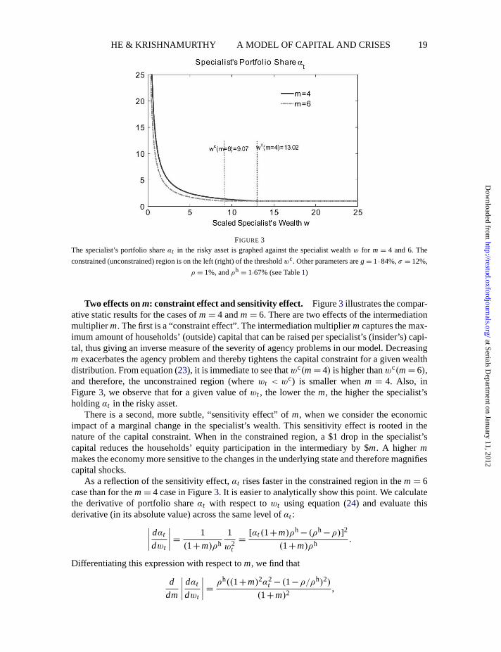
In Figure3, we plot the specialist’s portfolio shareαt in the risky asset against the scaledspecialist’s wealthwt . The specialist’s portfolio holding in the risky asset rises above 100%once the economy is in the constrained region and rises even higher when the specialist’ wealthfalls further. As a result, the risk exposure allocation, which departs from the first-best one, istilted towards the specialist who has relatively low wealth. Since in our model the specialist, notthe household, is in charge of the intermediary’s investment decisions, asset prices have to adjustto make the higher risk share optimal.
becomesmore constrained, the high risk aversion of the specialist causes the equilibrium risk premium to rise sufficientlyfast that the asset price falls. In the present model, if we set the discount rates equal to each other, although the riskpremium does rise as the specialist loses wealth, the interest rate also falls, and with log utility, these two effects offseteach other. To solve the model for the case of differential (in particular non-log) utility, we have to rely on numericalmethods inHe and Krishnamurthy(2010). Another way to introduce liquidation is to model a second-best buyer forthe risky asset. For example, suppose households can directly own the asset, but in doing so, receive a lower dividendthan specialists. Then, if the intermediation constraint binds sufficiently, the households will bypass the specialists todirectly purchase the asset. This modelling sets a lower bound at which the asset is liquidated to the households. Modelssuch asKiyotaki and Moore(1997) andKyle and Xiong(2001) have this feature. Following this approach in our settingnecessitates having to model bankruptcy and, in particular, the specialist’s trading decisions after bankruptcy. We do nottake this approach because it is sufficiently more complicated than the simple discount rate approach and it is unclear ifthe added complexity will yield more in terms of the substance of our analysis.
at Serials Departm
ent on January 11, 2012http://restud.oxfordjournals.org/
Dow
nloaded from
“rdr036” — 2011/11/11 — 17:41 — page 19 — #19
HE & KRISHNAMURTHY A MODEL OF CAPITAL AND CRISES 19
FIGURE 3The specialist’s portfolio shareαt in the risky asset is graphed against the specialist wealthw for m = 4 and 6. The
constrained (unconstrained) region is on the left (right) of the thresholdwc. Other parameters areg = 1∙84%,σ = 12%,
ρ = 1%, andρh = 1∙67% (see Table1)
Two effects onm: constraint effect and sensitivity effect. Figure3 illustrates the compar-ative static results for the cases ofm = 4 andm = 6. There are two effects of the intermediationmultiplier m. The first is a “constraint effect”. The intermediation multiplierm captures the max-imum amount of households’ (outside) capital that can be raised per specialist’s (insider’s) capi-tal, thus giving an inverse measure of the severity of agency problems in our model. Decreasingm exacerbates the agency problem and thereby tightens the capital constraint for a given wealthdistribution. From equation (23), it is immediate to see thatwc(m= 4) is higher thanwc(m= 6),and therefore, the unconstrained region (wherewt < wc) is smaller whenm = 4. Also, inFigure3, we observe that for a given value ofwt , the lower them, the higher the specialist’sholdingαt in the risky asset.
There is a second, more subtle, “sensitivity effect” ofm, when we consider the economicimpact of a marginal change in the specialist’s wealth. This sensitivity effect is rooted in thenature of the capital constraint. When in the constrained region, a $1 drop in the specialist’scapital reduces the households’ equity participation in the intermediary by $m. A higher mmakes the economy more sensitive to the changes in the underlying state and therefore magnifiescapital shocks.
As a reflection of the sensitivity effect,αt rises faster in the constrained region in them = 6case than for them = 4 case in Figure3. It is easier to analytically show this point. We calculatethe derivative of portfolio shareαt with respect towt using equation (24) and evaluate thisderivative (in its absolute value) across the same level ofαt :
∣∣∣∣dαt
dwt
∣∣∣∣=
1
(1+m)ρh
1
w2t
=[αt (1+m)ρh − (ρh −ρ)]2
(1+m)ρh.
Differentiating this expression with respect tom, we find that
d
dm
∣∣∣∣dαt
dwt
∣∣∣∣=
ρh((1+m)2α2t − (1−ρ/ρh)2)
(1+m)2,
at Serials Departm
ent on January 11, 2012http://restud.oxfordjournals.org/
Dow
nloaded from

“rdr036” — 2011/11/11 — 17:41 — page 20 — #20
20 REVIEW OF ECONOMIC STUDIES
which is positive for all relevant parameters (recall thatαt ≥ 1 andρh > ρ). In other words,whenm is higher, a change in specialist wealth leads to a larger change inαt . While we do notgo through the computations in the next sections, this sensitivity effect arises in most of the assetpricing measures that we consider.
The two effects ofm shed light on crises episodes and financial development. If we considerthat a developed economy like the U.S. has institutions with higherm’s, then our model predictsthat these institutions on average have more outside financing and less binding financing con-straints. Moreover, in the developed economies, crises episodes are unusual (constraint effect),but on incidence, are often dramatic (sensitivity effect).
4.4.3. Risky asset volatility. We may write the equilibrium evolution of the specialist’swealthWt as
dWt
Wt= μW,t dt +σW,t dZt , (25)
where the driftμW,t andthe volatilityσW,t areto be determined in equilibrium. By matching thediffusion term in equation (25) with the specialist’s budget equation (13), it is straightforward tosee that
σW,t Wt = E∗t σR,t . (26)
The dollar volatility of the specialist’s wealth is equal to the volatility of the risky asset returnmodulated by the risk exposure held by the specialist.
Given equation (22), the diffusion term on the risky asset price is
σR,t Pt = Vol(d Pt ) = σDt
ρh+(
1−ρ
ρh
)WtσW,t = σ
Dt
ρh+(
1−ρ
ρh
)E∗
t σR,t ,
which implies that
σR,t =σ Dt
ρhPt − (ρh −ρ)E∗t
. (27)
Substituting in forE∗t from Proposition5, we have the following proposition.
Proposition 7. In the unconstrained region,σR,t = σ . In the constrained region, we have
σR,t = σ
((1+m)ρh
mρh +ρ
)(1
1+ (ρh −ρ)wt
).
As Figure4 shows, in the unconstrained region, the volatility of the risky asset is constantand equal to dividend volatilityσ . The volatility rises in the constrained region as the constrainttightens (i.e.wt falls). In fact, in the constrained region,E∗
t = 11+m Pt , and equation (27) implies
that
σR,t =(
1
Pt/Dt
)
σ
ρh − ρh−ρ1+m
.
Therefore,the volatility σR,t increasesbecause the price/dividend ratioPt/Dt falls. The lattercondition is consistent with the fire-sale discount of the intermediated assets (see comments infootnote15).
The model can help explain the rise in volatility that accompanies periods of financial tur-moil where intermediary capital is low. It can also help explain the rise in the VIX index duringthese periods and why the VIX has come to be called a “fear” index. We will next show thatthe periods of low intermediary capital also lead to high expected returns. Taking these results
at Serials Departm
ent on January 11, 2012http://restud.oxfordjournals.org/
Dow
nloaded from

“rdr036” — 2011/11/11 — 17:41 — page 21 — #21
HE & KRISHNAMURTHY A MODEL OF CAPITAL AND CRISES 21
FIGURE 4The risky asset volatilityσR,t is graphed against the scaled specialist wealthwt for m = 4 and 6. The constrained
(unconstrained) region is on the left (right) of the thresholdwc. Other parameters areg = 1∙84%,σ = 12%,ρ = 1%,
andρh = 1∙67% (see Table1)
together, we provide one possible explanation for recent empirical observations relating the VIXindex and risk premia on intermediated assets.Bondarenko(2004) documents that the VIX in-dex helps explain the returns to many different types of hedge funds.Berndtet al. (2004) notethat the VIX index is highly correlated with the risk premia embedded in default swaps. Inboth cases, the assets involved are specialized and intermediated assets that match those of ourmodel.
We also derive the specialist’s wealth volatilityσW,t , which is useful in later discussions. Wecan derive this either using equation (26) or more directly by noting thatσW,t = αtσR,t . That is,the volatility of specialist wealth is the volatility of risky asset return (σR,t ) modulated by thespecialist’s equilibrium portfolio share in the risky asset (αt ).
Proposition 8. In the unconstrained region,σW,t = σ . In the constrained region,
σW,t = αtσR,t =σ
wt (mρh +ρ).
4.4.4. Risk premium. The key observation regarding our model is that the specialist isin charge of the investment decisions into the risky asset. Asset prices then have to be such thatit is optimal for specialists to buy the market-clearing amount of risk exposure.
We can solve out for the risk premium in two ways. We know that
E∗t =
πR,t
σ 2R,t
Wt .
Using the market-clearing exposure stated in Proposition5 and the result ofσ 2R,t in Proposition
7, we can derive the risk premium.
at Serials Departm
ent on January 11, 2012http://restud.oxfordjournals.org/
Dow
nloaded from

“rdr036” — 2011/11/11 — 17:41 — page 22 — #22
22 REVIEW OF ECONOMIC STUDIES
Alternatively, and more directly, standard asset pricing arguments imply thatπR,t = αtσ2R,t .
We have just derived the equilibrium portfolio shareαt as well as the risky asset volatility. As aresult, we have the following proposition.
Proposition 9. In the unconstrained region,πR,t = σ 2. In the constrained region, we have
πR,t =(
σ 2
wt
)(1
1+ (ρh −ρ)wt
)((1+m)ρh
(mρh +ρ)2
).
The risk premium on the risky asset rises through the constrained region, as shown inFigure5. The higher risk premium is necessary to induce the specialists, who have low wealthand therefore low risk capacity, to buy the exposure. It is easy to show that this pattern alsoprevails for the Sharpe ratio.
An interesting point of comparison for our results is to the literature on state-dependent riskpremia, notably,Campbell and Cochrane(1999) andBarberis, Huang and Santos(2001). In thesemodels, as in ours, the risk premium is increasing in the adversity of the state. In Campbell andCochrane, the state dependence arises because marginal utility is dependent on the agent’s con-sumption relative to his habit stock. In Barberis, Huang, and Santos, the state dependence comesabout because risk aversion is modelled directly as a function of the previous period’s gains andlosses. Relative to these two models, we work with a standard Constant Relative Risk Aversionutility function but generate state dependence endogenously as a function of the frictions in theeconomy.
Our model is closer in spirit to heterogeneous agent models where losses shift wealth be-tween less and more risk-averse agents thereby changing the risk aversion of the representativeinvestor.Kyle and Xiong(2001) andLongstaff and Wang(2008) are examples of this work. InKyle and Xiong(2001), the two agents are a log investor and a long-term investor. Althoughtheir paper is not explicit in modelling the preferences and portfolio choice problem of the
FIGURE 5Risk premiumπR,t is graphed against the scaled specialist wealthwt for m = 4 and 6. The constrained (unconstrained)
region is on the left (right) of the thresholdwc. Other parameters areg = 1∙84%,σ = 12%,ρ = 1%, andρh = 1∙67%
(see Table1)
at Serials Departm
ent on January 11, 2012http://restud.oxfordjournals.org/
Dow
nloaded from

“rdr036” — 2011/11/11 — 17:41 — page 23 — #23
HE & KRISHNAMURTHY A MODEL OF CAPITAL AND CRISES 23
long-term investor, since his demand function is different than the log investor, implicitly hischoices must reflect different preferences.
In theoretical terms, our model also works through shifts in wealth between household andspecialist. However, both agents in our model share the same utility function, so the action israther through the capital constraint and its effect on market participation. We elaborate on thispoint next.
4.4.5. Agency and risk aversion. A principal theoretical contribution of our paper rel-ative to prior work is that we show how variation in the risk aversion embodied in the pricingkernel can be explained by agency problems, rather than to particular aspects of household pref-erences. In particular, the risk premium in Proposition9 is a function ofm in the constrainedregion. We can rewrite the risk premium in Proposition9 as
πR,t =(
σ 2
wt
)(1
1+ (ρh −ρ)wt
)((mρh +ρ)+ (ρh −ρ)
(mρh +ρ)2
).
Thelast term in parentheses depends onm: asm decreases (i.e.the agency friction tightens), therisk premium rises. The effect is only present in the constrained region since the risk premiumis constant in the unconstrained region .
We can investigate this comparative static exercise further in our model. It is plausible thatmoral hazard problems themselves vary so that there are times,e.g.during a financial crisis, inwhichm is particularly low.16 We now consider a variation of our model in whichm is stochastic:
dmt
mt= σmdZm
t ,
whereσm is a positive constant and{Zmt } is another Brownian process independent of{Zt }.
Here,dZmt capturesthe shocks to agency frictions, and a negative shock (d Zm
t < 0) lowersmtandtherefore leads to more severe agency problems. We calld Zm
t the moral hazard factor inthis economy.
We show that in AppendixA.6 that the equilibrium policy and pricing expressions for theeconomy with a stochasticm are the same as those that we have derived for the case of a constantm, with the only adjustment of replacingm with mt . The key to this result is the assumptionof log preferences. With log preferences, the price/dividend ratio is not a function ofm (seeequation (22)). As a result, the shockd Zm
t doesnot affect the return dynamics of the asset.Moreover, given the log preferences, agents choose their optimal consumption and portfoliopolicies myopically. In particular, the possibility that equilibrium prices or policies in the futuremay depend on the future dynamics ofmt doesnot affect equilibrium choices today. Hence, theproblem reduces to a static problem given today’s value ofmt .
With these points in mind, consider the behaviour of the risk premium in response to theagency shocksd Zm
t . In the unconstrained region, the risk premium is constant,πR,t = σ 2, whichis independent ofmt andtherefored Zm
t . In the constrained region, the risk premium is (replacingm by mt )
πR,t =(
σ 2
wt
)(1
1+ (ρh −ρ)wt
)((mtρ
h +ρ)+ (ρh −ρ)
(mtρh +ρ)2
).
16. Variation in m may be because moral hazard is more severe during crises or becausem itself depends onmonitoring by large investors as inHolmstrom and Tirole(1997).
at Serials Departm
ent on January 11, 2012http://restud.oxfordjournals.org/
Dow
nloaded from

“rdr036” — 2011/11/11 — 17:41 — page 24 — #24
24 REVIEW OF ECONOMIC STUDIES
FIGURE 6The loading of risk premiumπR,t on the agency factord Zm
t is graphed against the scaled specialist wealthwt when
mt = 4, for the case ofρ = ρh = 1∙67% andρ = 10%,ρh = 1∙67%. The constrained (unconstrained) region is on the
left (right) of the thresholdwc. Other parameters areg = 1∙84%,σ = 12%, andσm = 10%
We use Ito’s lemma to differentiate this expression. For the special case thatρ = ρh, the depen-dence on the moral hazard factor is transparent:17
dπR,t = d
(σ 2
wt (mt +1)ρ
)= −
σ 2
w2t (mt +1)ρ
dwt −σ 2
wt (mt +1)2ρdmt + dt terms.
This result shows that a positive shock todmt (or the moral hazard factord Zmt ) reducesπR,t ,
while a negative shock increasesπR,t . That is, shocks tomt mimic shocks to the “risk aversion”of the financial intermediary.
Interestingly, the impact of the moral hazard shock increases with the tightness of the capitalconstraint. Figure6 illustrates this effect, graphing the loading of the risk premium on the moralhazard factord Zm
t . The loading is negative because an increase in moral hazard corresponds toa decrease inmt . We draw the graph both for theρ = ρh case as well as for the usualρh > ρcase. Intuitively, the root of the capital constraint is the agency friction. As a result, when theeconomy is more constrained, it is also more sensitive to the alleviation or worsening of theagency friction.
For the rest of the paper, for simplicity, we return to the case of a constantm. In the ap-pendix, we provide expressions for all of our asset pricing results for both the constantm andthe stochasticm.
4.4.6. Exposure price and intermediation fee. We now calculate the equilibrium expo-sure pricekt . As noted earlier, the fee is zero in the unconstrained region. For the constrainedregion, equating the exposure demand (11) with exposure supply (21) and usingWh
t = Pt − Wt ,
17. The expression in the text omits terms of the order ofdt. Further, in AppendixA.6, we also show thatCov(dwt ,dmt ) = 0.
at Serials Departm
ent on January 11, 2012http://restud.oxfordjournals.org/
Dow
nloaded from

“rdr036” — 2011/11/11 — 17:41 — page 25 — #25
HE & KRISHNAMURTHY A MODEL OF CAPITAL AND CRISES 25
we have
Eh∗t (kt ) =
πR,t −kt
σ 2R,t
Wht = m
πR,t
σ 2R,t
Wt = mE∗t
⇒ kt =Wh
t −mWt
Wht
πR,t =Pt − (1+m)Wt
Pt − WtπR,t . (28)
And, we have
qt =πR,t
σ 2R,t
mkt = kt ∙mαt ,
which says that the equilibrium fee per unit of specialist’s capital (q) is the exposure price(kt ) multiplied by the total exposure (that households gain through intermediaries) per unit ofspecialist’s capital (mαt ). Rewriting in terms of primitives, we have the following theorem.
Proposition 10. In the unconstrained region, the exposure price kt = qt = 0. In the constrainedregion, the exposure price is
kt =1− (ρ +mρh)wt
1−ρwt
σ 2
wt (mρh +ρ)
((1+m)ρh
mρh +ρ
)(1
1+ (ρh −ρ)wt
)> 0
and
qt =πR,t
σ 2R,t
mkt =mσ 2
(ρ +mρh)2
1− (ρ +mρh)wt
1−ρwt
(1
wt
)2
> 0.
In Figure7, the exposure pricekt and the per-unit-of-wealth feeqt display a similar patternas the risk premium in Figure5. This is intuitive: the higher risk premium in the constrainedregion implies a higher household demand for investment in intermediaries to gain access to the
FIGURE 7Exposure pricekt (the left panel) and per-unit-of-specialist-wealth feeqt (the right panel) are graphed against the scaled
specialist wealthwt for m = 4 and 6. The constrained (unconstrained) region is on the left (right) of the thresholdwc.
Other parameters areg = 1∙84%,σ = 12%,ρ = 1%, andρh = 1∙67% (see Table1)
at Serials Departm
ent on January 11, 2012http://restud.oxfordjournals.org/
Dow
nloaded from

“rdr036” — 2011/11/11 — 17:41 — page 26 — #26
26 REVIEW OF ECONOMIC STUDIES
risky asset. Because the supply is fixed atmE∗t , the equilibrium exposure price rises to clear the
intermediation market.The rising fee on the specialists’ wealth is a reflection of the scarcity of the specialists’
capital.18 This underscores one of the key points of our model: intermediation capital becomesincreasingly valuable in a crisis when the intermediary sector suffers more losses. The followingexample illustrates this point.
Example: lending spreads and market liquidityDuring periods of financial turmoil in the intermediary sector, the terms of credit for new
loans get worse; seeGilchrist and Zakrajsek(2010) for empirical evidence. That is, lendingspreads rise, even on relatively safe borrowers. Our model sheds light on this phenomenon. Wenow interpret the intermediary as not just a purchaser of secondary market assets but also alender in the primary market (e.g.commercial banks). Suppose that a borrower (infinitesimal)asks the intermediary for a loan at datet to be repaid at datet + dt, with zero default risk. Wedenote the interest rate on this loan asr t andask whatrt lenderswill require.
Suppose that making the loan uses up capital. That is to say, if a specialist makes a loan of sizeδ, he has less wealth (Wt −δ) available for coinvestment with the household in the intermediary.In particular, if in the constrained region, the lender is able to attractmδ less funds from thehouseholds.19
If mWt > Wht , intermediation capital is not scarce and thusr t = rt . However, if interme-
diation capital is scarce, then using intermediation capital on the loan reduces the size of theintermediary. A lender could have used theδ in the intermediary to purchase the riskless bondyielding rt and received a fee from households ofqtδ. Since both investments are similarlyriskless, we must have that
r t = rt +qt .
Therefore,the lending spreadrt − rt risesonce we fall into the constrained region.In this example, even a no-default-risk borrower is charged the extra spread ofqt . The reason
is that the specialist intermediary is marginal in pricing the loan to the new borrower, so thatthe opportunity cost of specialist capital is reflected in the lending spread. If we had assumedthat households could also have made such a loan, then we will find thatr t = rt . Of course abusiness loan, which requires expertise and knowledge of borrowers, is the prime example of anintermediated investment.20
18. The higher intermediation transfer from households to specialists is the logical result of our model of scarcesupply of intermediation. However, it seems counterfactual that specialists can demand a higher fee from their investorsduring a crisis period in which agency concerns may be widespread. One resolution of this anomalous result is to assumethat households, lacking the knowledge of the risky asset market, are also not aware of time variation in the risk premiumon the risky asset. For example, one can explore a model in which households hold static beliefs over the mean–varianceratio of the pay-offs delivered by intermediaries. This model may deliver the result that fees are state independent,thereby resolving the counterfactual result on fees. We do not pursue this extension here.
19. To develop this example in terms of the primitive incentive constraint, we need to assume that households onlyobserve the specialist’s wealth net of the loan and do not observe the actual loan. Also, households’ beliefs are thatevery specialist will contribute his entire wealth into the intermediary when the delegation fee is positive, a belief thatis consistent with the current equilibrium. In this case, observing wealth ofWt − δ leadshouseholds to believe that therisk exposure delivered by that specialist is reduced proportionately, which in turn tightens the intermediation capacityconstraint.
20. The results illustrated in this example are also present in the model ofHolmstrom and Tirole(1997), althoughthe connection to secondary market activity is not apparent in their model.
at Serials Departm
ent on January 11, 2012http://restud.oxfordjournals.org/
Dow
nloaded from
“rdr036” — 2011/11/11 — 17:41 — page 27 — #27
HE & KRISHNAMURTHY A MODEL OF CAPITAL AND CRISES 27
4.4.7. Interest rate and flight to quality. We can derive the equilibrium interest ratertfrom the household’s Euler equation, which is
rtdt = ρhdt +Et
[dch∗
t
ch∗t
]−Vart
[dch∗
t
ch∗t
].
Theequilibrium condition gives us
dch∗t
ch∗t
=d(ρhWh
t )
ρhWht
=d(Pt − Wt )
Pt − Wt.
Recallthat the specialist’s budget equation is
dWt/Wt = αt (dRt − rtdt)+ rtdt −ρdt +qtdt .
Using the expressions forαt , σR,t , andqt thathave been derived previously, we have the follow-ing proposition.
Proposition 11. In the unconstrained region, the interest rate is
rt = ρh + g+ρ(ρ −ρh)wt −σ 2.
In the constrained region, the interest rate is
rt = ρh + g+ρ(ρ −ρh)wt −σ 2
[ρ((1+m)
( 1wt
−ρ)−m2ρh
)+ (mρh)2
]
(1−ρwt )(ρ +mρh)2.
In the unconstrained region, the interest rate is decreasing in the scaled specialist’s wealthwt . This just reflects the divergence in both parties’ discount rates (recall thatρ < ρh). In thelimiting case whereWt = Dt
ρ , the economy only consists of specialists. Then consistent with thefamiliar result of an economy with specialists as representative log investors, the interest rateconverges toρ + g−σ 2. For a smallerwt , where households play a larger part of the economy,the bond’s return also reflects the households’ discount rateρh, and the equilibrium interest rateis higher.
In the constrained region, the pattern is reversed: the smaller the specialist’s wealth, thelower the interest rate. This is because the capital constraint brings about two effects that rein-force each other. First, when the capital constraint is binding, the result in Proposition8 impliesthat the specialists bear disproportionately greater risk in this economy: the specialist’s wealthvolatility increases dramatically and more so when the specialist’s wealth further shrinks. As aresult, the volatility of the specialist’s consumption growth rises, and the precautionary savingseffect increases his demand for the riskless bond. Second, as specialist wealth falls, householdswithdraw equity from intermediaries and channel these funds into the riskless bond. The extrademand for bonds from both specialist and households lowers the equilibrium interest rate.
The pattern of decreasing interest rate presented in Figure8 is consistent with a “flight toquality”. Households withdraw funds from intermediaries and increase their investment in bondsin response to negative price shocks. This disintermediation leaves the intermediaries more vul-nerable to the fundamental asset shocks.
4.4.8. Illiquidity and correlation. In the capital constrained region, an individual spe-cialist who may want to sell some risky asset faces buyers with reduced capital. Additionally,
at Serials Departm
ent on January 11, 2012http://restud.oxfordjournals.org/
Dow
nloaded from

“rdr036” — 2011/11/11 — 17:41 — page 28 — #28
28 REVIEW OF ECONOMIC STUDIES
FIGURE 8Interest ratert is graphed against the scaled specialist wealthwt for m= 4 and 6. The constrained (unconstrained) region
is on the left (right) of the thresholdwc. Other parameters areg = 1∙84%,σ = 12%,ρ = 1%, andρh = 1∙67% (see
Table1)
since households reduce their (indirect) participation in the risky asset market, the set of buyersof the risky asset effectively shrinks in the constrained region. In this sense, the market for therisky asset “dries up”. On the other hand, if a specialist wished to sell some bonds, then thepotential buyers include both specialists as well as households. Thus, the bond is more liquidthan the risky asset.
There are further connections we can draw between low intermediary capital and aggregateilliquidity periods. As we have already seen, a negative shock in the constrained region leadsto a rise in risk premia, volatility, and fall in interest rate. In this subsection, we show that ourmodel also generates increasing comovement of assets that many papers have documented asan empirical regularity during periods of low aggregate liquidity (see,e.g.Chordia, Roll andSubrahmanyam, 2000). We illustrate this point through two examples.
Example 1: orthogonal dividend processWe introduce a second asset held by the intermediaries.21 This asset is a noisy version of the
market asset. The asset is in infinitesimal supply so that the endowment process and the equilib-rium wealth process for specialists are unchanged. In particular, we assume that the dividend onthis second asset is
dDt
Dt= gdt+σd Zt + σdZt =
d Dt
Dt+ σdZt .
Here,{Zt } is the common factor modelled earlier and{Zt } is a second Brownian motion, or-thogonal to{Zt }, which captures the asset’s idiosyncratic variation. Put differently, this secondasset is a noisy version of the market asset.
21. If the asset was traded by both households and specialists, then its introduction will have an effect on equilib-rium since the market is incomplete. However, introducing an intermediated asset will not alter the equilibrium.
at Serials Departm
ent on January 11, 2012http://restud.oxfordjournals.org/
Dow
nloaded from

“rdr036” — 2011/11/11 — 17:41 — page 29 — #29
HE & KRISHNAMURTHY A MODEL OF CAPITAL AND CRISES 29
FIGURE 9The correlation between the market return and the return on an individual asset, corr(d Rt , ˆd Rt ), is graphed against the
scaled specialist wealthw for m = 4 and 6. The constrained (unconstrained) region is on the left (right) of the threshold
wc. Other parameters areg = 1∙84%,σ = 12%,ρ = 1%,ρh = 1∙67% (see Table1), andσ = 12%
We can show that the price of this second asset is22
Pt = DtPt
Dt= Dt
[1
ρh+(
1−ρ
ρh
)wt
]. (29)
Consider the correlation betweend Rt and the return ˆd Rt on the second asset:
corr(d Rt , ˆd Rt ) =1
√1+ (σ /σR,t )2
.
In the unconstrained region, sinceσR,t is a constant, the correlation is constant. But, in theconstrained region, asσR,t rises, the common component of returns on the two assets becomesmagnified, causing the assets to become more correlated. We graph this state-dependent corre-lation in Figure9, where we simply takeσ = σ .
Example 2: liquidation-sensitive assetThe preceding example illustrates how the risk price of a common dividend rises during
crises periods and causes increased comovement in asset prices. Another mechanism for co-movement that is often emphasized by observers centres on forced liquidations by constrainedintermediaries. The following example illustrates this case.
22. Given the guessed form in equation (29), PtDt
= PtDt
, which implies thatdPtPt
= d PtPt
+ d(Dt /Dt )
Dt /Dt= d Pt
Pt+ σdZt .
Therefore,dRt = DtPt
+ dPtPt
= d Rt + σdZt . Then we can verify that it satisfies the specialist’s Euler equation
qt dt −ρdt +Et
[dc∗tc∗t
]+Vart
[dc∗tc∗t
]+Et [d Rt ] = Covt
[dc∗tc∗t
,dRt
].
at Serials Departm
ent on January 11, 2012http://restud.oxfordjournals.org/
Dow
nloaded from

“rdr036” — 2011/11/11 — 17:41 — page 30 — #30
30 REVIEW OF ECONOMIC STUDIES
We model a liquidation-sensitive asset as an asset with a dividend that drops (discontinu-ously) from unity to an exogenously specified fire-sale value, which we normalize to zero, wheneconomy-wide intermediary capital falls beneath a thresholdW. When intermediary capital issufficiently low, therefore, forced liquidation becomes more likely. This lowers the liquidation-sensitive asset’s price. As we have shown, low intermediary capital also pushes down the valueof the market asset. Thus, at a low enough intermediary wealth, the returns on the market assetand liquidation-sensitive asset move together.
Normalize the initial date as time 0 with the state pair(W0, D0 = 1). Consider an (infinites-imal) asset that pays offXT at the maturity dateT , where the dividend is state-contingent,i.e.XT = X(WT , DT ). We are interested in how the economy-wide shocks drive the asset price,when the asset is subject to forced liquidation. We assume that the dividendX(WT , DT ) isreceived only if the economy-wide intermediary capitalWT at the maturity date is above a min-imum thresholdW:
X(WT , DT ) =
{1 if WT > W,
0 otherwise.
This asset reflects an investment-grade corporate bond or a mortgage-backed security that isat low risk during normal times. However, during a period of low intermediation capital, theasset value is determined by an exogenous fire-sale value, which we have normalized to be zero.Denote the time-0 price of this liquidation-sensitive asset asQ0(W, D) = Q0(W0,1), whichis simply the time-0 present value ofX(WT , DT ) under the pricing kernel in this economy. Wefocus on the constrained region to illustrate the interesting dynamics in this example and performthe computations numerically.
FIGURE 10The instantaneous covariance between the returns of intermediated market asset and the liquidation-sensitive asset,
i.e. cov(d R,d Q0(W0,1)). The x-horizontal is the time-0 specialist’s wealthw = W0, as we normalizeD0 = 1. We
takem = 4, so the capital constraint binds atwc = 13. The liquidation threshold isW = 3∙57. Other parameters are
g = 1∙84%,σ = 12,ρ = 1%, andρh = 1∙67% (see Table1)
at Serials Departm
ent on January 11, 2012http://restud.oxfordjournals.org/
Dow
nloaded from

“rdr036” — 2011/11/11 — 17:41 — page 31 — #31
HE & KRISHNAMURTHY A MODEL OF CAPITAL AND CRISES 31
The value of this liquidation-sensitive zero-coupon bondQ0(W0,1) varies with the state ofthe economy. Interestingly, the sign of the correlation switches depending on the state. Considera negative shock to this economy causing intermediary capitalWt to fall. A lower Wt leadstoa lower interest rate in the constrained region, which in turn leads to a higher bond price. Thisinterest rate effectgenerates a negative correlation between the returns of our (intermediated)market risky asset and the liquidation-sensitive asset.
When the intermediary capitalW0 is sufficiently low, i.e. in the vicinity of the liquidationboundaryW, an oppositeliquidation effectkicks in. Under this effect, a negative shock makesforced liquidation more likely, and the price of the liquidation-sensitive asset falls. As a result,there is positive correlation between the market return and the asset return.
Figure10 graphs the instantaneous covariance betweend Q0(W0,1) andthe market returnd Rt . When the scaled specialist’s wealth is high, the correlation is negative, although close tozero for the parameters in our example. The covariance becomes more negative asW0 shrinksdueto the interest rate effect. Finally, whenW0 falls aroundW (which is 3∙57 in our example),the liquidation effect dominates, and the liquidation-sensitive asset comoves with the intermedi-ated market asset.
5. DISCUSSION OF INTERMEDIATION CONTRACT
In this section, we discuss in further detail the contracting issues that arise in our model.
5.1. Discussion of incentive constraint
We think of the incentive constraint that emerges from the model as similar to the explicit andimplicit incentives across many modes of intermediation. For example, a hedge fund manageris typically paid 20% of the return on his fund. We may think of this 20% as corresponding tothe minimum fractionβ that has to be paid to the hedge fund manager for incentive provisionpurposes. Likewise, many investment and commercial banks have traders on performance-basedbonus schemes. Mutual funds receive more flows if they generate high returns (Warther, 1995),and the salaries of the managers of these funds rise with the fees on these flows. Thus, there is arelation between the pay-offs to the manager and the returns on the mutual fund. Finally, whilethese examples all have the agent exposed to returns on the upside, it is also true that agents whogenerate poor returns are fired or demoted.
The key feature of the model, which we think is robustly reflected across many modes ofintermediation in the world, is the feedback between losses suffered by an intermediary (drop inWt ) and exit by the investors of that intermediary. Our model captures this feature through thecapital constraint, when it is binding.
5.2. Benchmarking
A substantive restriction that we impose on the contracting space is to not consider benchmark-ing contracts. In our model, the specialist is compensated/punished based only on his own per-formance; we do not consider contracts where one specialist’s performance is benchmarked tothe aggregate risky asset return and/or the performance of another specialist. If we allow for suchcontracts, then the principal can perfectly detect shirking by the agent. As such, the principal canovercome the moral hazard problem at no cost.
The issue of benchmarking is a thorny one for macroeconomic models of credit market fric-tions.23 Froma theoretical standpoint, the literature has offered some avenues to explicitly deal
23. For example, the analysis of the model ofHolmstrom and Tirole(1997) turns on comparative statics of inter-mediaries’ total capital to shed light on a credit crunch. However, if we interpret these changes in intermediary capital
at Serials Departm
ent on January 11, 2012http://restud.oxfordjournals.org/
Dow
nloaded from

“rdr036” — 2011/11/11 — 17:41 — page 32 — #32
32 REVIEW OF ECONOMIC STUDIES
with the benchmarking issue. We think the most promising for our model is based on the limited-commitment models of,e.g.Kehoe and Levine(1993) and the diversion models of,e.g.DeMarzoand Fishman(2007). For example, consider a model in which the agent (specialist) can divertsome investment returns at a cost into his personal account. Moreover, as in Kehoe and Levine,even though such diversion is observable, there are no courts that can punish detectable diver-sion. In this case, one can imagine that the principal will commit to a contract whereby the agentis paid a share of the investment return if the agent does not divert. The share is chosen to be largeenough so as to eliminate the incentive to divert. In this formulation, even if all agents generatehigh returns (i.e. a good aggregate shock), a given agent still needs to be bribed with a share ofhis (higher aggregate) returns to prevent diversion. Thus, the agent receives payments that varywith the aggregate state. The reason this modelling can work is that in Kehoe and Levine, theincentive constraint isex post.
Is it easy to accommodate this change within our model? The answer is yes for the equitycontract of the model. The harder issue is the debt contract. In our model, shorting the bond (i.e.borrowing) is not affected by agency issues. This assumption is consistent with our effort moralhazard formulation and allows our analysis to focus on the effect of constraining a single equitymargin. With the possibility of diversion, presumably debt borrowings will also be constrained(see footnote8). Thus, we would have to study a model with constraints on both equity and debt.While such a model seems both theoretically and empirically interesting to study, we leave thistask for future work.
5.3. Long-term contracts
For tractability reasons, in this paper we focus on short-term contracts. There has been muchrecent interest in dynamic models of long-term financial contracts,e.g.DeMarzo and Fishman(2007),Biais et al. (2007), andDeMarzo and Sannikov(2006). In these models, the principalcommits to a compensation rule as a function of the agent’s performance history. In our model,no party can commit beyond the short-term intermediation relationship [t, t +dt].
On the one hand, it will be interesting to develop models that marry the dynamic financialcontracting models with the dynamic asset pricing models. We are unaware of papers in theliterature that accomplish this. On the other hand, if the main advantage of long-term contract-ing is to generate history dependence, then it is worth noting that in our model the special-ist’s compensation—and in turn the aggregate state—is history dependent despite the short-termnature of the intermediation relationship. History dependence arises in our model because weembed the short-term contracting problem into a dynamic model.
In particular, in our model, after the intermediary sector suffers a series of losses, the special-ists’ wealth drops faster than that of the households.24 As a result, the agency frictions becomemore severe, which is reflected in a more distorted risk allocation towards the intermediary sectorwith scarce capital. This is akin to the result inDeMarzo and Fishman(2007),Biaiset al.(2007),
asthe result of exogenous aggregate shocks, then in a full-blown dynamic model, presumably agents will write contractsthat anticipate these shocks. In general, such contracts will condition out the aggregate shocks (seeKrishnamurthy,2003). Of course, in practice, we think that the Holmstrom–Tirole comparative static based on intermediation capitalis still interesting; these aggregate shocks apparently do affect intermediation capacity. Our model allows us to see thevarious asset pricing effects of this “comparative static” within a dynamic model. Thus, we view our model as the logicaldynamic extension of the Holmstrom–Tirole analysis.
24. This occurs when the economy starts from the constrained region where the specialists own a leveraged posi-tion in the risky asset. If the economy starts from the unconstrained region, becauseρh > ρ, households consume morerelative to the specialists, and as a result, the economy eventually reaches the constrained region. InHe and Krishna-murthy(2010), we introduce leverage in the unconstrained region so that both regions are transient.
at Serials Departm
ent on January 11, 2012http://restud.oxfordjournals.org/
Dow
nloaded from

“rdr036” — 2011/11/11 — 17:41 — page 33 — #33
HE & KRISHNAMURTHY A MODEL OF CAPITAL AND CRISES 33
andDeMarzo and Sannikov(2006), where a sequence of bad performance shocks increases thelikelihood of inefficient termination/liquidation. The underlying connection is that in both mod-els, after a sequence of bad shocks, the agent’s inside stake within the relationship (whether it isshort-term or long-term) falls, leading to more severe agency frictions.
5.4. Observability of specialist portfolio
We assume that the specialist’s portfolio choice is unobservable. We make this assumptionprimarily because it seems in harmony with the household limited-participation assumption.Households who lack the knowledge to directly invest in the risky asset market are also unlikelyto understand how specialists actually choose the intermediaries’ portfolio.
On the other hand, making the portfolio choice observable will not substantively affect any ofour results. The AppendixA.7 formally solves the case where the portfolio choice is observable,but the due-diligence effort problem remains. Relative to the case of unobservable portfoliochoice, the main difference is that now the household pays intermediation fees to the specialistthat depend on the actual risk exposure delivered to the household. In other words, when theportfolio choice is observable, from the specialist’s point of view the total intermediation fee isno longer a function of his wealth; rather, it becomes a direct function of the exposure supply tothe household.25
The region of interest is the constrained region, where in our current model the householdachieves a lower-than-first-best exposure to the risky asset. In this region, the sharing ruleβt isstill binding at the constant1
1+m to respect the incentive-compatibility constraint, regardless ofwhether the portfolio choice is observable or not. Therefore, in light of equations (6) and (7), inequilibrium, we still have
Eh∗t = mE∗
t .
We know from equation (11) that the households demandEh∗t is decreasing inkt . In our current
model where the portfolio choice is unobservable, the exposure supplymE∗t is independent ofkt
(seeequation (21)). Now in the case of observable portfolio choice, the exposure supplymE∗t is
increasingin kt (seeequation (A.10) in AppendixA.7). Intuitively, with a positive risk exposurepricekt , specialists are induced to supply more exposure to households. Because the supply isnot infinitely elastic, the core feature of inefficient risk allocation is preserved in the observableportfolio choice case: the risk-sharing allocation tilts towards more risk on the specialist, ex-actly as the unobservable portfolio choice case (see Proposition6 in Section4.4). The lower thespecialist’s wealth (or intermediary capital)Wt , the tighter is the intermediation constraint, andtherefore, the more inefficient the risk allocation in this economy. Again, to induce the specialistto hold the equilibrium risky asset position, the risk premium rises accordingly. Therefore, thelink between the extent of the capital constraint and the higher risk premium is preserved in theobservable portfolio choice case.
5.5. Non-linear contracts
We have restricted attention to affine contracts(βt , Kt ) in solving for an intermediation con-tract. It is worth asking how our results will be altered if we considered non-linear contracts
25. In the main model with unobservable portfolio choice, it is the specialist’s observable wealth that determinesthe actual risk exposure supply in the constrained region. As a result, even though the household purchases risk exposurefrom the intermediary, the total fee is a function of specialist’s wealth. Any specialist can potentially promise to delivera higher-than-equilibrium level of risk exposure to households in an attempt to earn greater total intermediation fees.However, because the investment position is unobservable, this promise is not credible.
at Serials Departm
ent on January 11, 2012http://restud.oxfordjournals.org/
Dow
nloaded from
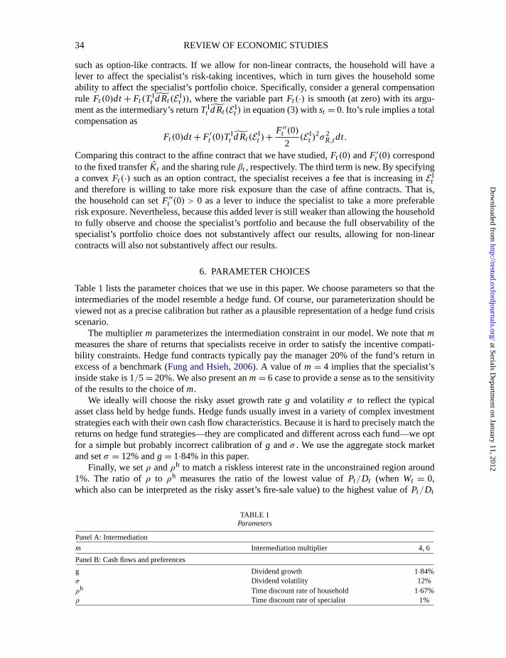
“rdr036” — 2011/11/11 — 17:41 — page 34 — #34
34 REVIEW OF ECONOMIC STUDIES
such as option-like contracts. If we allow for non-linear contracts, the household will have alever to affect the specialist’s risk-taking incentives, which in turn gives the household someability to affect the specialist’s portfolio choice. Specifically, consider a general compensationrule Ft (0)dt + Ft (T I
t dRt (E It )), where the variable partFt (∙) is smooth (at zero) with its argu-
ment as the intermediary’s returnT It dRt (E I
t ) in equation (3) withst = 0. Ito’s rule implies a totalcompensation as
Ft (0)dt + F ′t (0)T I
t dRt (EIt )+
F ′′t (0)
2(E I
t )2σ 2
R,t dt .
Comparing this contract to the affine contract that we have studied,Ft (0) andF ′t (0) correspond
to the fixed transferKt andthe sharing ruleβt , respectively. The third term is new. By specifyinga convexFt (∙) suchas an option contract, the specialist receives a fee that is increasing inE I
tand therefore is willing to take more risk exposure than the case of affine contracts. That is,the household can setF ′′
t (0) > 0 as a lever to induce the specialist to take a more preferablerisk exposure. Nevertheless, because this added lever is still weaker than allowing the householdto fully observe and choose the specialist’s portfolio and because the full observability of thespecialist’s portfolio choice does not substantively affect our results, allowing for non-linearcontracts will also not substantively affect our results.
6. PARAMETER CHOICES
Table1 lists the parameter choices that we use in this paper. We choose parameters so that theintermediaries of the model resemble a hedge fund. Of course, our parameterization should beviewed not as a precise calibration but rather as a plausible representation of a hedge fund crisisscenario.
The multiplierm parameterizes the intermediation constraint in our model. We note thatmmeasures the share of returns that specialists receive in order to satisfy the incentive compati-bility constraints. Hedge fund contracts typically pay the manager 20% of the fund’s return inexcess of a benchmark (Fung and Hsieh, 2006). A value ofm = 4 implies that the specialist’sinside stake is 1/5 = 20%. We also present anm = 6 case to provide a sense as to the sensitivityof the results to the choice ofm.
We ideally will choose the risky asset growth rateg and volatility σ to reflect the typicalasset class held by hedge funds. Hedge funds usually invest in a variety of complex investmentstrategies each with their own cash flow characteristics. Because it is hard to precisely match thereturns on hedge fund strategies—they are complicated and different across each fund—we optfor a simple but probably incorrect calibration ofg andσ . We use the aggregate stock marketand setσ = 12% andg = 1∙84% in this paper.
Finally, we setρ andρh to match a riskless interest rate in the unconstrained region around1%. The ratio ofρ to ρh measuresthe ratio of the lowest value ofPt/Dt (when Wt = 0,which also can be interpreted as the risky asset’s fire-sale value) to the highest value ofPt/Dt
TABLE 1Parameters
Panel A:Intermediation
m Intermediationmultiplier 4, 6
Panel B: Cash flows andpreferences
g Dividend growth 1∙84%σ Dividend volatility 12%ρh Time discount rate of household 1∙67%ρ Time discount rate of specialist 1%
at Serials Departm
ent on January 11, 2012http://restud.oxfordjournals.org/
Dow
nloaded from

“rdr036” — 2011/11/11 — 17:41 — page 35 — #35
HE & KRISHNAMURTHY A MODEL OF CAPITAL AND CRISES 35
(when Wht = 0). We set this ratio to be 60% to be loosely consistent with the Warren Buf-
fett/AIG/Goldman Sachs bid for the Long-term Capital Management (LTCM) portfolio in fallof 1998.26
7. CONCLUSION
We have presented a model to study the effects of capital constraints in the intermediary sectoron asset prices. Capital effects arise because (1) households lack the knowledge to participatein the risky asset and (2) intermediary capital determines the endogenous amount of exposurethat households can achieve to the risky asset. The model builds on an explicit microeconomicfoundation for intermediation. The model is also cast within a dynamic economy in which onecan articulate the dynamic effects of capital constraints on asset prices. We show that the modelcan help to explain the behaviour of asset markets during aggregate liquidity events.
There are a number of interesting directions to take this research. First, the model we havepresented has a degenerate steady-state distribution, which means that we cannot meaningfullysimulate the model. For typical parameter values, the specialist will eventually end up with allthe wealth. This aspect of the model is well known and arises in many two-agent models (seeDumas,1989, for further discussion).He and Krishnamurthy(2010) analyse a closely relatedmodel, which has a non-degenerate steady-state distribution. That model is sufficiently complexthat it does not allow for the simple closed-form solutions of this paper. There, we solve themodel numerically and simulate to compute a number of asset pricing moments.
A second avenue of research is to expand the number of traded assets. Currently, the onlynon-intermediated asset in the model is the riskless bond. However, in practice, even unsophis-ticated households have the knowledge to invest in many risky assets directly or to invest in lowintermediation-intensive assets such as an S&P 500 index fund. It will be interesting to introducea second asset in positive supply in which households can directly invest and study the differ-ential asset pricing effects across these different asset classes. This exercise seems particularlyrelevant in light of the evidence in the fall of 1998 that it was primarily the asset classes investedin by hedge funds that were affected during the crises. Likewise, in the current credit crisis,intermediated debt markets were heavily affected since August 2007, while the S&P500 wasnot affected until September 2008. These observations suggest a richer channel running fromintermediated markets to non-intermediated markets. We intend to investigate these issues morefully in future work.
APPENDIX A
A.1. Proof of Lemma2
For simplicity, we omit time subscript underE , β, and K in this proof. With a slight abuse of notation, denote byE I (E I′ ) the intermediary’s optimal position (chosen by the specialist) in the risky asset given a contract5 = (β, K )
(5′ = (β ′, K ′)).First,we fix K = K ′ at the equilibrium level. Then it is obvious to see that the specialist will set
E I =E∗
βand E I′ =
E∗
β ′
underthese two contracts so that his effective risk exposureE∗ = βE I = E I′β ′ remainsthe same.
26. The Warren Buffett/AIG/Goldman Sachs bid was reported to be $4 billion for a 90% equity stake, suggesting aliquidation value of $4∙44 billion for LTCM’s assets. LTCM was said to have lost close to $3 billion of capital at the timeof this bid, suggesting that LTCM lost 40% of its value to arrive at the liquidation price of $4∙44 billion. Our calculationhere is clearly rough.
at Serials Departm
ent on January 11, 2012http://restud.oxfordjournals.org/
Dow
nloaded from
“rdr036” — 2011/11/11 — 17:41 — page 36 — #36
36 REVIEW OF ECONOMIC STUDIES
Next we argue that, for anyβ ∈[ 1
1+m ,1], it never pays to induce the specialist to choose a different portfolio by
raising the transferK above the equilibrium level (loweringK will lose the specialist to other households.) Giving thespecialist a larger transferK (ε) = K + ε reduces the household’s value at the order ofJh
W(Wht )εdt . Next, consider the
benefit to the household from the induced change in the specialist’s desired exposure. Fix future equilibrium policies.RaisingK by ε at timet raises the specialist’s wealth byεdt. According to the assumption that the specialist’s optimalrisk exposure is differentiable in his wealth, there exists some smooth functionH that the specialist will raise theexposureE∗ to
E∗() = H(Wt + εdt) = E∗ + H ′(Wt )εdt ,
which is higher thanE∗ in an order ofdt. Because the household’s value derived from his risk exposureEh = 1−ββ E
∗
is at most in the order ofdt(in fact the gain is
[JhW ∙ πR,tE
h + 12(Eh)2σ2
R,t JhWW
]dt), the total continuation value
increment by havingEh(ε) = 1−ββ E
∗(ε) relative toE∗ is bounded by the order of(dt)2. Therefore, it is not profitableto affect the exposure through the transferK . Finally, note that although we restrict our attention to transfersKdt in ourcontracting space, this argument also goes through if transfers are allowed to be in the order ofO(1). ‖
A.2. Proof of Lemma3
For simplicity, we omit time subscript underE , β, andK in this proof. We borrow from thecore’s “equal-treatment”property in the study of the equivalence between the core and Walrasian equilibrium (seeMas-Colell, Whinston andGreen,1995, Chapter 18, Section 18.B). Suppose that the equilibrium is asymmetric, and we have a continuum of(Eh(i ), K (i ))
(notethatEh = 1−β
β E∗ soessentially we have a continuum of different contracts(β(i ), K (i ))
), wherei
is the identity of the household–specialist pair. Choose the household who is doing the worst by getting some exposureEh′ andpaying a feeK ′ (seethe definition in Step 3 below) and match him with the specialist who is doing the worst,i.e. receiving the lowest feeK ′′ = mini K (i ). We want to show that this household–specialist pair can do strictly betterby matching and forming an intermediation relationship.
Define the average allocation(Eh, K ) as
εh ≡∫Eh(i )di and K ≡
∫K (i )di .
There are three observations.
1. (Eh, K ) is feasible. BecauseEh(i ) = 1−β(i )β(i ) E
∗, whereE∗ is constant for all specialists, andβ(i ) ≤ 11+m for all
i ’s, we candefineβ ≤ 11+m suchthat
1−β
β=∫
1−β(i )
β(i )di .
This impliesthatEh is achieved when setting the sharing rule tobeβ.2. The specialist is obviously weakly better offsinceK ≥ minK (i ).3. We want to show that the household is weakly better off. The household’s value can be written as
Uh(Eh(i ), K (i )) = Et [ln cht +e−ρhdt Jh(Wh
t+dt )] (A.1)
as a function of(Eh(i ), K (i )), where
Wht+dt = (1+ rt dt)Wh
t −cht dt +Eh(i )(dRt − rt dt)− K (i )dt,
and Jh(Wht+dt ) is the household’s continuation value as a function of wealth att + dt. The household who is
doing the worst has a valueUh′ ≡ min
iUh(i ).
By expandingUh(Eh, K ) in equation (A.1) and isolating terms affected by(Eh, K ), we see that maximizing thehousehold’s value is equivalent to maximizing
[(Eh(μR − rt ))Jh
W(Wht )− K +
1
2(Eh)2σ2
R,t JhWW(Wh
t )
],
where JhW(Wh
t ) and JhWW(Wh
t ) are the first- and second-order derivatives ofJh(∙), respectively. SinceJhWW(Wh
t ) < 0, this term is globally concave in(Eh, K ) and strictly concave inEh. Therefore, the averageallocation yields a higher-than-average value
Uh(Eh, K ) ≥∫
Uh(i )di .
But becauseUh′ = mini Uh(i ) ≤
∫Uh(i )di , we have the desired resultUh(Eh, K ) ≥ Uh′.
at Serials Departm
ent on January 11, 2012http://restud.oxfordjournals.org/
Dow
nloaded from

“rdr036” — 2011/11/11 — 17:41 — page 37 — #37
HE & KRISHNAMURTHY A MODEL OF CAPITAL AND CRISES 37
Finally, note that if(Eh(i ), K (i ))’s are not identical across individual pairs, then at least one of the inequalitiesestablished above is strict. Therefore,(Eh, K ) blocksthe original asymmetric coalition.‖
A.3. Proof of Proposition1
The proof is similar to the proof of Proposition2, with θt =πR,t −kt
σR,tandrt = rt . ‖
A.4. Proof of Proposition2
We use the martingale method ofCox and Huang(1989) to derive the optimal consumption–portfolio choices. Thespecialist budget equation evolves according to
dWt = Et (dRt − rt dt)+qt Wt dt + Wtrt dt −ct dt
= Et (dRt +qt dt − (rt +qt )dt)+ (rt +qt )Wt dt −ct dt . (A.2)
We can redefine the return processes as
dRt ≡ dRt +qt = (μR,t +qt )dt +σR,t dZt ≡ μR,t dt +σR,t dZt and r t ≡ rt +qt
andwritedWt = Et (dRt − r t dt)+ r t Wt dt −ct dt .
Define the effective Sharpe ratio as
θt ≡μR,t − r t
σR,t=
πR,t
σR,t,
andthe relevant deflator is defined as
ξt = exp
[−∫ t
0rsds−
∫ t
0θsdZs −
1
2
∫ t
0θ2s ds
]> 0,
with dξt = −ξt (rt dt + θt dZt ). Then the dynamic problem in equation (17) is simplified to the following static problem:
maxctE[∫ ∞
0e−ρt lnct dt
]
s.t. W0 ≥ E[∫ ∞
0ξt ct dt
].
Clearly, the budget constraint should bind in optimal solution. Letλ be the LaGrange multiplier. Then the solution is
e−ρt
λξt= c∗
t , (A.3)
with λ = 1ρW0
. Because
Wt =1
ξtEt
[∫ ∞
tξscsds
]=
1
ξtEt
[∫ ∞
t
e−ρs
λds
]=
e−ρt
λξtρ,
combiningwith equation (A.3), we havec∗t = ρWt . (A.4)
Standard verification argument implies that the above First-order condition is sufficient for optimality. For the optimalportfolio choice, note that the deflated wealth process
Wt ξt = Et
[∫ ∞
tξsc∗
sds
]= Et
[∫ ∞
t
e−ρs
λds
]=
e−ρt
λρ
is deterministic, which implies that under the optimal portfolio strategy the local diffusion term ofWt ξt hasto be zero.Focusing on diffusion terms, we havedWt = E∗
t σR,t dZt anddξt = −ξt θt dZt .Therefore,the local diffusion terms ofWt ξt mustsatisfy
dWt ∙ ξt + Wt ∙ dξt
= (ξtE∗t σR,t − Wt ξt θt )dZt = 0,
at Serials Departm
ent on January 11, 2012http://restud.oxfordjournals.org/
Dow
nloaded from
“rdr036” — 2011/11/11 — 17:41 — page 38 — #38
38 REVIEW OF ECONOMIC STUDIES
which implies that(recall θt =
πR,tσR,t
)
E∗t = Wt
θt
σR,t= Wt
πR,t
σ2R,t
. (A.5)
The following value function approach shows that the specialist’s continuation value is log in his own wealth. Thisverifies the regularity conditions that we used in proving Lemmas 1, 2, and 3. Guess the specialist’s value function as
J(Wt ,Y(wt )) = Y(wt )+1
ρlnWt ,
whereY is a function of the aggregate statewt = WtDt
, whereWt is the aggregate specialists’ wealth. The specialist’sHamilton-Jacobi-Bellman (HJB) equation is
ρ
(Y(wt )+
1
ρlnWt
)= max
ct ,Et
lnct +μY,t+
(Et (μR,t − rt )+ (qt + rt )Wt −ct )JW(Wt )+ 12E
2t σ2
R,t JWW(Wt )
= maxct ,Et
{lnct +μY,t+
(Et (μR,t − rt )+ (qt + rt )Wt −ct )1
ρWt− 1
2E2t σ2
R,t1
ρW2t
}
, (A.6)
where
μY,t ≡ Y′(wt )μw,t +1
2Y′′(wt )σ
2w,t and σY,t ≡ Y′(wt )σw,t . (A.7)
The first-order conditions for policies{c∗t ,E∗
t } yields
c∗t = ρWt and E∗
t =πR,t
σ2R,t
Wt ,
sameas what we derived under the Cox–Huang approach. Plugging the above two results into equation (A.6), collectingterms, and combining with equation (A.7), we can characterizeY(wt ) (althoughthis characterization is unnecessary forour main analysis).27 ‖
A.5. Sufficient conditions for suboptimality of implementing shirking
We give sufficient conditions under which implementing shirking is suboptimal. We take the result in Lemma2 as given,especially the agents’ continuation value along the equilibrium path.
Consider any contract(β ′t , K ′
t ). Suppose that the household implements shirkingst = 1. The household’s dynamicbudget equation when implementingst = 1 is
dWht
∣∣∣st =1
= (1−β ′t )E
It (dRt − rt dt)− K ′
t dt + Wht rt dt −ch
t dt − (1−β ′t )Xt dt ,
whereβ ′t < 1
1+m , while when implementingst = 0, it is
dWht
∣∣∣st =0
= (1−βt )EIt (dRt − rt dt)− Kt dt + Wh
t rt dt −cht dt .
Clearly, the household faces the trade-off that (1) he gains by getting a greater risk exposure by settingβ ′t < 1
1+m , but(2) he suffers a deterministic cost of−K ′
t − (1−β ′t )Xt + Kt .
27. Using the dynamics of aggregate specialists’ wealthWt , one can derived(wt ) = d(Wt
Dt
)= μw,t dt +σw,t dZt ,
whereμw,t ≡ wt(π2
R,t
σ2R,t
+qt + rt −ρ +σ2−g−πR,tσR,t
σ), andσw,t ≡ wt
(πR,tσR,t
−σ). This implies thatY(w) satisfies the
following second-order ordinary differential equation:
Y′(wt )μw,t +1
2Y′′(wt )σ
2w,t = ρY(wt )− lnρ +
1
ρ
[1
2
(πR,t
σR,t
)2+qt + rt −ρ
]
.
at Serials Departm
ent on January 11, 2012http://restud.oxfordjournals.org/
Dow
nloaded from

“rdr036” — 2011/11/11 — 17:41 — page 39 — #39
HE & KRISHNAMURTHY A MODEL OF CAPITAL AND CRISES 39
Let us first bound the household’s gain due to a greater risk exposure. The HJB equation for household is (similarto equation (A.6))
ρh(
Yht +
1
ρhlnWh
t
)
= maxcht ,Eh
t
[lnch
t +μYh,t + (Eht (μR − rt −kt )+ rt W
ht −ch
t )JhW(Wh
t )+1
2(Eh
t )2σ2R,t Jh
WW(Wht )
].
To compare the equilibrium flow benefit of risk exposure when implementing working and shirking, we isolate the
terms withEht . When working is implemented, we setEh∗
t =πR,t −kt
σ2R,t
Wht andsubstitute formulas fromJh
W(Wht ) and
JhWW(Wh
t ) from the proof of Proposition 2, which gives the flow benefit of
1
2ρ
(μR,t − rt −kt
σR,t
)2.
Whenshirking is implemented, the upper bound flow benefit under the optimal risk exposure is12ρ
(μR,t −rtσR,t
)2. There-
fore, the incremental benefit due to a greater risk exposure is bounded by (using the result ofσ2R,t , kt , andπR,t in
Section4.4)
1
2ρ
[(μR,t − rt
σR,t
)2−(
μR,t − rt −kt
σR,t
)2]
=1
2ρ
kt (2πR,t −kt )
σ2R,t
=σ2
2ρw2t
(1− (ρ +mρh)wt )(1−ρwt +mρh)
(mρh +ρ)2(1−ρwt )2.
(A.8)Now, we study the cost side. When implementing shirking, the specialist understands that shirking brings a total ofBt − β ′
t Xt benefit(loss if negative) to his own account. Since the specialist’s receives a fee ofKt in equilibrium bytaking other contracts that implementst = 0, the household has to pay at leastK ′
t = Kt − Bt +β ′t Xt to the specialist.
Therefore, the total incremental loss (we assume thatXt = (1+m)Bt throughout)is
− (Kt − Bt +β ′t Xt )− (1−β ′
t )Xt + Kt = Bt − Xt = −m
1+mXt . (A.9)
Therefore, as long asm1+m Xt dominatesthe increment benefit in equation (A.8) (which depends on our primitive pa-
rameters and the endogenous aggregate statewt ), implementing shirking is never optimal.‖
A.6. Proof of stochastic mt in Section4.4.5
With stochasticm as dmtmt
= σmdZmt , we have the same pricing function
Pt
Dt=
1
ρh+(
1−ρ
ρh
)wt ,
with wt = Wt/Dt . The reason is that we derive this price/dividend ratio only based on log preferences and market-clearing conditions, and it is independent of agency frictions (check the argument in Section4.4.1). Note that since theprice/dividend ratio does not depend onmt , the asset return does not directly depend ond Zm
t shocks,i.e.
d Rt =dPt + Dt dt
Pt= μR,t dt +σR,t dZt .
Given this result, we show that the equilibrium under stochasticmt is the equilibrium solved in the baseline model, withthe only adjustment of replacingm with mt
Becausethe asset return does not depend ond Zmt , the specialist’s budget equation is the same as before:
dWt/Wt = rt dt +αtπR,t dt +αtσR,t dZt −ρdt +qt dt ,
which implies thatdwt = d(Wt
Dt
)is uncorrelated withd Zm
t locally. The standard optimal portfolio decision requires that
αt =πR,t
σ2R,t
, which holds under the proposed equilibrium. For interest rate, we derive the equilibrium interest ratert from
at Serials Departm
ent on January 11, 2012http://restud.oxfordjournals.org/
Dow
nloaded from

“rdr036” — 2011/11/11 — 17:41 — page 40 — #40
40 REVIEW OF ECONOMIC STUDIES
Uncon.Region Con. Region
E∗t Wt
11+mt
Pt
αt 1 1+(ρh−ρ)mt(1+mt )ρhmt
σR,t σ σ1+(ρh−ρ)wt
((1+mt )ρ
h
mt ρh+ρ
)
πR,t σ2 σ2
wt (mt ρh+ρ)
((1+mt )ρ
h
mt ρh+ρ
)(1
1+(ρh−ρ)mt
)
kt 0 1−(ρ+mt ρh)wt
(1−ρwt )(1+(ρh−ρ)wt )
(1+mt )ρhσ2
wt (mt ρh+ρ)2
rt ρh + g−σ2 +ρ(ρ −ρh)wt ρh + g+ρ(ρ −ρh)wt −σ2
[ρ((1+mt )
(1
wt−ρ
)−m2
t ρh)+(mt ρ
h)2]
(1−ρwt )(ρ+mt ρh)2
thehousehold’s Euler equation:
rt dt = ρhdt +Et
[dch∗
t
ch∗t
]
−Vart
[dch∗
t
ch∗t
]
= ρhdt +Et
[d(Pt − Wt )
Pt − Wt
]−Vart
[d(Pt − Wt )
Pt − Wt
].
Becauseboth dWt anddPt do not involved Zmt shocks,the same calculation applies. Finally, we check equilibrium
fees. Recall that we determine fees by using the intermediation clearing condition:
Eh∗t (kt ) =
πR,t −kt
σ2R,t
Wht = mt
πR,t
σ2R,t
Wt = mtE∗t ⇒ kt =
Wht −mt Wt
Wht
πR,t =Pt − (1+mt )Wt
Pt − WtπR,t ,
whichgives the formula in the table.
A.7. Observable portfolio choice
Suppose that the portfolio choice is observable. The competitive intermediation market—where the households arepurchasing risk exposure from specialists—is identical to a standard goods market analysis. The household pays thespecialist based on the exposure that the specialist delivers. Importantly, this implies that the total fee is then linear inthe exposure supply so thatKt = ktEh
t , wherekt is the price per-unit of exposure that the household receives. This is incontrast to our current case where the specialist’s exposure is not directly observable and the households have to inferthe exposure supply from the specialist’s wealth.
In this case, the specialist understands that his choice of risk exposureEt deliversmEt units of exposure to thehousehold, which brings a total fee ofmktEt dt (this also applies to the unconstrained region wherekt = 0). Therefore,the specialist’s budget equation is (for a comparison, check equation (18))
dWt = Et (dRt − rt dt)+mktEt dt + Wtrt dt −ct dt ,
where the second termmktEt dt captures the total intermediation fee. Clearly, this quantity-based transfer will affect thespecialist’s optimal portfolio choiceE∗
t . Now the specialist’s HJB equation is (whereYt is a function of aggregate satesand prices),
ρ
(Yt +
1
ρlnWt
)= max
ct ,Et
[
lnct +μY,t + (EtπR,t +mktEt + rt Wt −ct )1
ρWt−
1
2E2
t σ2R,t
1
ρW2t
]
,
sowe havec∗t = ρWt and
E∗t =
πR,t +mkt
σ2R,t
Wt . (A.10)
at Serials Departm
ent on January 11, 2012http://restud.oxfordjournals.org/
Dow
nloaded from

“rdr036” — 2011/11/11 — 17:41 — page 41 — #41
HE & KRISHNAMURTHY A MODEL OF CAPITAL AND CRISES 41
In fact, equation (A.10) is the only change in the unobservable portfolio choice case(recall that in the observable case,
E∗t =
πR,t
σ2R,t
Wt is independent ofkt). The decision rule for the household is still the same as in the case with unobservable
portfolio choice,i.e. ch∗t = ρWh
t andEh∗t =
πR,t −kt
σ2R,t
Wht .
Thekey moral hazard agency friction still applies in this case, which implies that
Eh∗t ≤ mE∗
t . (A.11)
In other words, in order for the specialist to not shirk, he has to bear at least11+m of the risk of the intermediary.
We can provide explicit solutions in this case. In the unconstrained region, whether the portfolio choice is observableor not makes no difference:kt = 0, and we still have the first-best risk sharing as in the unobservable case. Consider theconstrained region. We repeat the steps of Section4.4 in the paper. Risky asset price is the same:
Pt =Dt
ρh+(
1−ρ
ρh
)Wt .
Thespecialist’s exposureE∗t , portfolio positionαt , andσR,t remainthe same. It is because in the main text we have just
used the market-clearing condition and capital constraint to derive these four objects, and the issue of observability isirrelevant.
On the other hand, since the observability does affect the specialist’s portfolio decision, the equilibrium risk pre-mium changes accordingly. Now we have
Eh∗t =
πR,t −kt
σ2R,t
Wht = mE∗
t = mπR,t +mkt
σ2R,t
Wt .
UsingE∗t +Eh∗
t = P, we can obtain
kt =Pt − (1+m)Wt
Pt − Wt +m2WtπR,t (A.12)
and
πR,t =Pt − Wt +m2Wt
(1+m)(Pt − Wt )
σ2
wt (mρh +ρ)
((1+m)ρh
mρh +ρ
)(1
1+ (ρh −ρ)wt
).
Thisdiffers from the result in the unobservable case (28) by a factor of
Pt − Wt +m2Wt
(1+m)(Pt − Wt )=
Pt/Dt −wt +m2wt
(1+m)(Pt/Dt −wt )< 1,
implying that observability does ease the constraint. However, whenWt → 0, this factor Pt −Wt +m2Wt(1+m)(Pt −Wt )
→ 11+m , there-
foreπR,t is still in the order of 1wt
. This implies that the key asset pricing implication, which comes from the distortionin risk sharing, remains the same in the observable case. We then can solve forkt basedon equation (A.12), which isalso in the order of1wt
asin the unobservable case. Finally, we can solve for interest ratert asin Section4.4.7.
Acknowledgment.We thank Andrea Eisfeldt, Oleg Bondarenko, Bruno Biais, Darrell Duffie, Mike Fishman,Jonathan E. Ingersoll, Ravi Jagannathan, Haitao Li, John Moore, Andrew Nowobilski, Andrea Prat, Dimitri Vayanos,Adrien Verdelhan, Wei Xiong, three anonymous referees and participants at seminars at Northwestern, London Schoolof Economics, University of Illinois at Chicago, NBER Summer Institute, China International Conference in Finance2006, and Stanford Institute for Theoretical Economics 2006, Society of Economic Dynamics 2009, Yale FinancialCrisis Conference 2009, and Massachusetts Institute of Technology for helpful comments.
REFERENCES
ADRIAN, T., ETULA, E. and MUIR, T. (2011), “Financial Intermediaries and the Cross-Section of Asset Returns”,(Working Paper, Northwestern University).
ALLEN, F. and GALE, D. (1994), “Limited Market Participation and Volatility of Asset Prices”,American EconomicReview, 84, 933–955.
ALVAREZ, F., ATKESON, A. and KEHOE, P. (2002), “Money, Interest Rates, and Exchange Rates with EndogenouslySegmented Markets”,Journal of Political Economy, 110, 73–112.
BARBERIS, N., HUANG, M. and SANTOS, T. (2001), “Prospect Theory and Asset Price”,The Quarterly Journal ofEconomics,116, 1–53.
at Serials Departm
ent on January 11, 2012http://restud.oxfordjournals.org/
Dow
nloaded from

“rdr036” — 2011/11/11 — 17:41 — page 42 — #42
42 REVIEW OF ECONOMIC STUDIES
BASAK, S. and CUOCO, D. (1998), “An Equilibrium Model with Restricted Stock Market Participation”,Review ofFinancial Studies, 11, 309–341.
BATES, D. (2003), “Empirical Option Pricing: A Retrospection”,Journal of Econometrics, 116, 387–404.BERNDT, A., DOUGLAS, R., DUFFIE, D., FERGUSON, M. and SCHRANZ, D. (2004), “Measuring Default Risk
Premia from Default Swap Rates and EDFs” (Mimeo, Stanford University).BIAIS, B., MARIOTTI, T., PLANTIN, G. and ROCHET, J. (2007), “Dynamic Security Design: Convergence to Con-
tinuous Time and Asset Pricing Implications”,Review of Economic Studies,74, 345–390.BONDARENKO, O. (2004), “Market Price of Variance Risk and Performance of Hedge Funds” (Mimeo, University of
Illinois-Chicago).BRUNNERMEIER, M. K. and PEDERSEN, L. H. (2008), “Market Liquidity and Funding Liquidity”,Review of Finan-
cial Studies,22, 2201–2238.BRUNNERMEIER, M. and SANNIKOV, Y. (2010), “A Macroeconomic Model of Financial Sector” (Working Paper,
Princeton University).CAMPBELL, J. and COCHRANE, J. (1999), “By Force of Habit: A Consumption-Based Explanation of Aggregate
Stock Market Behavior”,Journal of Political Economy, 107, 205–251.CHORDIA, T., ROLL, R. and SUBRAHMANYAM, A. (2000), “Commonality in Liquidity”,Journal of Financial
Economics,56, 3–28.COLLIN-DUFRESNE, P., GOLDSTEIN, R. and MARTIN, J. (2001), “The Determinants of Credit Spread Changes”,
Journal of Finance,66, 2177–2207.COX, J. and HUANG, C. (1989), “Optimal Consumption and Portfolio Policies when Asset Prices Follow a Diffusion
Process”,Journal of Economic Theory, 49, 33–83.DEMARZO, P. and FISHMAN, M. (2007), “Optimal Long-Term Financial Contracting”,Review of Financial Studies,
20, 2079–2128.DEMARZO, P. and SANNIKOV, Y. (2006), “Optimal Security Design and Dynamic Capital Structure in a Continuous-
Time Agency Model”,Journal of Finance, 61, 2681–2724.DIAMOND, D. and RAJAN, R. (2005), “Liquidity Shortages and Banking Crises”,Journal of Finance,60, 615–647.DUFFIE, D. (2010), “Asset Price Dynamics with Slow-Moving Capital”,Journal of Finance, 65, 1238–1268.DUFFIE, D. and STRULOVICI, B. (2011), “Capital Mobility and Asset Pricing” (Working Paper, Stanford University).DUMAS, B. (1989), “Two-Person Dynamic Equilibrium in the Capital Market”,Review of Financial Studies, 2,
157–188.EDMOND, C. and WEILL, P. (2009), “Aggregate Implications of Micro Asset Market Segmentation” (Working Paper
No. 15254, NBER).FROOT, K. (2001), “The Market for Catastrophe Risk: A Clinical Examination”,Journal of Financial Economics,60,
529–571.FROOT, K. and O’CONNELL, P. (1999), “The Pricing of US Catastrophe Reinsurance”, in Froot, K. (ed.)The Financing
of Catastrophe Risk(Chicago: University of Chicago Press).FUNG, W. and HSIEH, D. (2006), “Hedge Funds: An Industry in Its Adolescence”,Federal Reserve Bank of Atlanta
Economic Review, 91, 1–33.GABAIX, X., KRISHNAMURTHY, A. and VIGNERON, O. (2007), “Limits of Arbitrage: Theory and Evidence from
the MBS Market”,Journal of Finance, 62, 557–596.GARLEANU, N., PEDERSON, L. and POTESHMAN, A. (2009), “Demand-Based Option Pricing”,Review of Finan-
cial Studies, 22, 4259–4299.GEANAKOPLOS, J. and FOSTEL, A. (2008), “Leverage Cycles and the Anxious Economy”,American Economic
Review, 98, 1211–1244.GILCHRIST, S. and ZAKRAJSEK E. (2010), “Credit Spreads and Business Cycle Fluctuations”,American Economic
Review, forthcoming.GROMB, D. and VAYANOS, D. (2002), “Equilibrium and Welfare in Markets with Financially Constrained Arbi-
trageurs”,Journal of Financial Economics, 66, 361–407.HE, Z. and KRISHNAMURTHY, A. (2010), “Intermediary Asset Pricing” (Working Paper, Chicago Booth and North-
western University).HOLMSTROM, B. and TIROLE, J. (1997), “Financial Intermediation, Loanable Funds, and the Real Sector”,Quarterly
Journal of Economics, 112, 663–691.KEHOE, T. and LEVINE, D. (1993), “Debt-Constrained Asset Markets”,Review of Economic Studies, 60, 865–888.KIYOTAKI, N. and MOORE, J. (1997), “Credit Cycles”,Journal of Political Economy, 105, 211–248.KRISHNAMURTHY, A. (2003), “Collateral Constraints and the Amplification Mechanism”,Journal of Economic The-
ory, 111, 277–292.KYLE, A. and XIONG, W. (2001), “Contagion as a Wealth Effect”,Journal of Finance, 56, 1401–1440.LONGSTAFF, F. and WANG, J. (2008), “Asset Pricing and the Credit Market” (Working Paper, MIT).LUCAS, R. (1978), “Asset Prices in an Exchange Economy”,Econometrica,46, 1429–1445.MANKIW, G. and ZELDES, S. (1991), “The Consumption of Stockholders and Non-stockholders”,Journal of Financial
Economics,29, 97–112.MAS-COLELL, A., WHINSTON, M. and GREEN, J. (1995),Microeconomic Theory(New York: Oxford University
Press).MITCHELL, M., PEDERSEN, L. and PULVINO, T. (2007), “Slow Moving Capital”,American Economic Review
Papers and Proceedings, 97, 215–220.
at Serials Departm
ent on January 11, 2012http://restud.oxfordjournals.org/
Dow
nloaded from

“rdr036” — 2011/11/11 — 17:41 — page 43 — #43
HE & KRISHNAMURTHY A MODEL OF CAPITAL AND CRISES 43
PAVLOVA, A. and RIGOBON, R. (2008), “The Role of Portfolio Constraints in the International Propagation ofShocks”,Review of Economic Studies, 75, 1215–1256.
SHLEIFER, A. and VISHNEY, R. (1997), “The Limits of Arbitrage”,Journal of Finance,36, 35–55.VAYANOS, D. (2005), “Flight to Quality, Flight to Liquidity, and the Pricing of Risk” (Working Paper, LSE).VISSING-JORGENSEN, A. (2002), “Limited Asset Market Participation and the Elasticity of Intertemporal Substitu-
tion”, Journal of Political Economy, 110, 825–853.WANG, J. (1996), “The Term Structure of Interest Rates in a Pure Exchange Economy with Heterogeneous Investors”,
Journal of Financial Economics, 41, 75–110.WARTHER, V. (1995), “Aggregate Mutual Fund Flows and Security Returns”,Journal of Financial Economics,39,
209–235.XIONG, W. (2001), “Convergence Trading with Wealth Effects: An Amplification Mechanism in Financial Markets”,
Journal of Financial Economics, 62, 247–292.
at Serials Departm
ent on January 11, 2012http://restud.oxfordjournals.org/
Dow
nloaded from