A Mixed-Dimensionality Modeling Approach for Interaction ...
164
Marquee University e-Publications@Marquee Master's eses (2009 -) Dissertations, eses, and Professional Projects A Mixed-Dimensionality Modeling Approach for Interaction of Heterogeneous Steam Reforming Reactions and Heat Transfer Jeroen Valensa Marquee University Recommended Citation Valensa, Jeroen, "A Mixed-Dimensionality Modeling Approach for Interaction of Heterogeneous Steam Reforming Reactions and Heat Transfer" (2009). Master's eses (2009 -). Paper 17. hp://epublications.marquee.edu/theses_open/17
Transcript of A Mixed-Dimensionality Modeling Approach for Interaction ...

Marquette Universitye-Publications@Marquette
Master's Theses (2009 -) Dissertations, Theses, and Professional Projects
A Mixed-Dimensionality Modeling Approach forInteraction of Heterogeneous Steam ReformingReactions and Heat TransferJeroen ValensaMarquette University
Recommended CitationValensa, Jeroen, "A Mixed-Dimensionality Modeling Approach for Interaction of Heterogeneous Steam Reforming Reactions and HeatTransfer" (2009). Master's Theses (2009 -). Paper 17.http://epublications.marquette.edu/theses_open/17

A MIXED-DIMENSIONALITY MODELING APPROACH FOR INTERACTION OF HETEROGENEOUS STEAM REFORMING REACTIONS AND HEAT TRANSFER
by
Jeroen Valensa, B.S.M.E.
A Thesis submitted to the Faculty of the Graduate School, Marquette University,
in Partial Fulfillment of the Requirements for the Degree of Master of Science
Milwaukee, Wisconsin
December 2009

ABSTRACT A MIXED-DIMENSIONALITY MODELING APPROACH FOR INTERACTION OF HETEROGENEOUS STEAM REFORMING REACTIONS AND HEAT TRANSFER
Jeroen Valensa, B.S.M.E.
Marquette University, 2009
Hydrogen is most often produced on an industrial scale by catalytic steam methane reforming, an equilibrium-limited, highly endothermic process requiring the substantial addition of heat at elevated temperatures. The extent of reaction, or conversion efficiency, of this process is known to be heat transfer limited. Scaling the industrial process equipment down to the size required for small, compact fuel cell systems has encountered difficulties due to increased heat losses at smaller scales. One promising approach to effectively scale down the reforming process is to coat the catalyst directly onto the heat exchange surfaces of an integrated reactor/heat exchanger. In this way, heat can be effectively transferred to the catalytic reaction sites and conversion efficiency can be greatly improved.
Optimizing a small-scale integrated reactor requires an understanding of the interactions between the steam reformer reaction kinetics and the heat and mass transfer effects within the heat exchanger. Past studies of these interactions have predominantly focused on highly simplified flow channel geometries, and are unable to account for devices having augmented heat exchange surfaces. Full three-dimensional methods are possible, but require excessive computational resources.
In this work, a mixed-dimensionality modeling approach is developed in order to better address the problems posed by these integrated devices. This modeling approach is implemented using a commercially available thermal finite element code. The solid domain is modeled in three dimensions, while the fluid is treated as a one-dimensional plug flow. The catalyst layer is treated as a surface coating over the three-dimensional surfaces. A subroutine to solve the surface reaction kinetics using a LHHW kinetic model is developed and incorporated into the code in order to address the highly non-linear thermal/kinetic interactions. Validation of the modeling approach is accomplished through comparison of model results to test data obtained from an integrated reactor/heat exchanger test unit. Analysis of the results indicates that the modeling approach is able to adequately capture the complex interactions within the test unit.

iii
ACKNOWLEDGMENTS
Jeroen Valensa, B.S.M.E.
I would like to thank my thesis committee – Dr. S. Scott Goldsborough, Dr. John
Borg and Dr. Hyunjae Park. Your thorough review and suggestions helped to shape the
final end product of this thesis, and is much appreciated.
Annette Wolak was always there in the Mechanical Engineering office to make
sure that I complied with all of the requirements. Thank you, Annette, for all of your
assistance over these past several years.
I would like to thank Modine Manufacturing Company, and especially the Fuel
Cell Products Group, for financially supporting this work. Over the years I have been
blessed with managers who were very supportive of me in my efforts to complete this
thesis, and I am especially grateful to Mike Reinke, Mark Voss, Mark Baffa, Joe
Stevenson and Eric Steinbach for their support.
Adam Kimmel was both a professional colleague and a fellow grad student.
Thank you, Adam, for both your technical assistance and your moral support. Having
someone in the same boat as me to commiserate with certainly helped a lot.
I owe a debt of gratitude to Paul Barnard and Giles Hall for facilitating all of the
experimental testing, and to Dr. Liping Cao for her fine CFD work to determine Nusselt
number correlations.
Finally, a heartfelt thank-you to the most important people in my life – my three
boys, Colin, Darren and Preston, and my wonderful wife Amy. Thank you all for
supporting me, for believing in me, for letting me work on this thesis when I needed to,
and for not letting me quit.

iv
TABLE OF CONTENTS
ACKNOWLEDGMENTS ................................................................................................. iii
TABLE OF CONTENTS................................................................................................... iv
NOMENCLATURE .......................................................................................................... vi
1. INTRODUCTION / MOTIVATION............................................................................. 1
1.1 National Vision of a Hydrogen Economy........................................................ 1
1.2 Hydrogen Production Methods ........................................................................ 6
1.3 Process Intensification of Steam Methane Reforming................................... 10
1.4 Catalyzed Heat Exchange Surfaces ............................................................... 13
1.5 Need For Modeling Capabilities.................................................................... 15
1.6 Outline for the Thesis..................................................................................... 16
2. BACKGROUND ......................................................................................................... 18
2.1 Technical Background .................................................................................... 18
2.2 Review of Historical Approaches and State of the Art................................... 29
2.2.1 Model Dimensionality .................................................................... 30
2.2.2 Kinetics ............................................................................................ 42
2.2.3 Heat Transfer and Thermal Boundary Conditions.......................... 48
2.3 Problem Statement .......................................................................................... 53
3. APPROACH ................................................................................................................ 55
3.1 Overview of the Approach.............................................................................. 55
3.2 Detailed Description of the Modeling Approach........................................... 59
3.3 Detailed Description Of the Experimental Test Unit..................................... 72

v
3.4 Description of the Computational Model ...................................................... 82
3.5 Design Optimization Study............................................................................ 93
4. RESULTS .................................................................................................................... 97
4.1 Experimental Unit Test Results ...................................................................... 97
4.2 Reaction Calibration Sample Test Results.................................................... 105
4.3 Computational Model Results....................................................................... 107
4.4 Comparison of Computational and Experimental Results............................ 115
4.5 Factorial Study Results ................................................................................. 124
5. CONCLUSIONS AND RECOMMENDATIONS .................................................... 127
5.1 Conclusions.................................................................................................. 127
5.2 Recommendations for Future Work............................................................. 129
BIBLIOGRAPHY........................................................................................................... 131
APPENDIX A – DETERMINATION OF FIN CHANNEL NUSSELT NUMBER ..... 136
APPENDIX B – CODE FOR SOLVING SMR REACTION ........................................ 142

vi
NOMENCLATURE
A pre-exponential constant in Arrhenius equation Ac fluid cross-sectional area in flow channel Ai,j conductivity interaction factor for species i and j cp specific heat Dh hydraulic diameter Ea activation energy Fi molar flow rate of species i g acceleration due to gravity
Ti,g Gibbs function for species i at temperature T oTi,g molar Gibbs function for species i at temperature T and standard-state
pressure G Gibbs free energy GHSV Gas Hourly Space Velocity hf convective film coefficient
oTi,h molar enthalpy of species i at temperature T and standard-state pressure
ja mass flux of species a k kinetic rate factor ka rate of adsorption kinetic factor kd rate of desorption kinetic factor K equilibrium constant L conduction height of the fin Mi molecular weight of species i N number of moles Nu Nusselt number P pressure Pi partial pressure of species i Po standard-state pressure Pr Prandtl number Q rate of heat flow q′ rate of heat flow per unit length q ′′ rate of heat flow per unit area (heat flux) r, z spatial coordinates in axisymmetric polar coordinate system rn rate of reaction n Ru universal gas constant Ra Rayleigh number Re Reynolds number S:C steam to carbon ratio
oTi,s entropy of species i at temperature T and standard-state pressure
t time tfin fin thickness T temperature

vii
Tmc mixing-cup temperature Twall wall temperature v velocity V volume W mechanical work x, y, z spatial coordinates in cartesian coordinate system
4CHx extent of methane conversion
2COx extent of carbon dioxide conversion yi molar fraction of species i γ specific heat ratio ε fin efficiency η catalyst effectiveness factor ηf fin efficiency ηCarnot Carnot cycle efficiency ηOtto Otto cycle efficiency θ surface coverage µ dynamic viscosity λ thermal conductivity ρ density ρB catalyst bed density ωa mass fraction of species a Ω reactor cross-sectional area

1
1. INTRODUCTION / MOTIVATION
1.1 National Vision of a Hydrogen Economy
In November of 2001 the United States Department of Energy (DOE) initiated
work to develop a national vision of the United States’ transition towards a hydrogen
economy. This effort was driven by a variety of concerns regarding the traditional
energy infrastructure of the United States. The more notable of those concerns are the
national security implications of a heavily petroleum-dependant energy mix, and
environmental concerns over the byproducts and endproducts of fossil fuel utilization.
That this work by the DOE was initiated shortly after the events of September 11,
2001 was not merely coincidental. Those events sharply elevated the long-existent
concerns over U.S. energy security and the heavy dependence of the United States on
petroleum imports for its energy supply. While the gasoline shortages of the 1970’s first
alerted the nation to the possible downsides of being so dependant on imported fossil
fuels, it was not until the attacks of 9/11 that concerns over energy security became a
national priority. Over the past decade the United States has been spending in excess of
$200 billion annually on imported petroleum, and it is estimated that this number could
increase to $300 billion by 2030 (Hinkle & Mann, 2007). This magnitude of spending
does not include the indirect costs to the federal budget of the associated security and
diplomacy operations.

2
Hydrogen is seen as an alternative energy carrier that could be produced from a
variety of energy feedstocks, including domestically available alternatives to imported
petroleum, such as corn and other biomass crops. It has been estimated that, once the
technology has been fully developed and production facilities have been constructed
(approximately by 2030), hydrogen produced from coal could be used to fulfill about
15% of the light duty vehicle fuel needs in the United States, thereby replacing $25-$38
billion of imported oil with about $2.5 billion of domestic coal (Hinkle & Mann, 2007).
The combustion of fossil fuels for electricity generation and as a transportation
fuel inevitably results in a level of undesirable pollutant emissions being produced as
byproducts. The key emissions that have been identified as environmental pollutants that
must be reduced are SO2 (sulfur dioxide), NOx (oxides of nitrogen), mercury, CO (carbon
monoxide), and VOCs (volatile organic compounds) (National Energy Policy
Development Group [NEPDG], 2001). These pollutants have various negative impacts
on society. They have been associated with a variety of health issues such as respiratory
and cardiopulmonary disease, cancer, and birth defects, and have been found to cause
damage to forests, bodies of water, and the wildlife therein (NEPDG, 2001).
Ongoing efforts since the early 1970’s have significantly reduced the levels of
these key emissions – although the total U.S. energy consumption has increased by 42%
over the period from 1970 through 2000, the aggregate amount of key air emissions has
decreased by 31%. Nonetheless, the combustion of fossil fuels for energy production

3
continues to be the dominant source of these key pollutants in the United States (NEPDG,
2001).
Although concerns over undesirable pollutant byproducts of fossil fuels usage
have been prevalent for decades, the past several years have seen new concerns over the
production rates of CO2 (carbon dioxide), the natural end-product of any fossil fuel
combustion, due to its role as a greenhouse gas. Unlike pollutants, the emissions of
which can be theoretically reduced to zero levels through cleaner combustion, the CO2
produced by the use of fossil fuels can only be reduced to a finite level by increasing the
efficiency of the energy conversion process. Beyond increasing energy efficiency of
processes utilizing fossil fuels, the emission of CO2 into the atmosphere can be reduced
by sequestering the CO2 created in energy conversion processes, and by switching to
renewable sources of energy production.
An important distinction that is frequently made – and needs to be made –
between hydrogen and conventional energy sources such as fossil fuels, is that hydrogen
is in essence an energy carrier and not an energy source. Although hydrogen is the most
abundant element in the universe, it is virtually never found naturally occurring in its
molecular state on earth. Rather, it is most often encountered either bonded with oxygen
as water (H2O), or bonded with carbon in the form of hydrocarbons.
Molecular hydrogen can be reacted with the molecular oxygen that is abundantly
available in the earth’s atmosphere to form water. At standard temperature and pressure

4
(20°C and 101.325 kPa) and with the product water remaining in vapor form, this
chemical reaction releases 242 kJ of energy per mole of reacting hydrogen. Due to the
low molecular weight of hydrogen (2.016 grams per mole of molecular hydrogen), this
gives hydrogen a very high gravimetric energy density (120kJ/kg, relative to gasoline
which has an energy density of 44kJ/kg).
The most common manner by which the chemical energy stored in the molecular
bonds of a hydrogen molecule can be released is by combusting the hydrogen with
oxygen. Operating such a combustion process however will never allow for the full 242
kJ/mole to be realized as useful work, as stated by Carnot’s theorem. This theorem, first
proposed by Nicolas Léonard Sadi Carnot in 1824, states that the maximum efficiency of
a cycle which produces work by transferring heat from a reservoir at a fixed absolute
temperature TH to a reservoir at a lower fixed absolute temperature TL is the Carnot
efficiency, as shown in equation (1.1), with Qin being the amount of heat transferred and
Wnet, Carnot being the work produced.
high
low
in
Carnotnet,Carnot T
T1Q
Wη −≡= (1.1)
A cycle operating at such a Carnot efficiency would be operating reversibly, with
no net production of entropy internally. As such, the Carnot efficiency of a heat engine
operating by combusting hydrogen with oxygen can only be approached and never
reached.

5
It has been demonstrated that hydrogen can be used as a fuel within an internal
combustion engine (U.S. Department of Energy, 2002b). In such an engine, the
theoretical efficiency that can be attained is that of the Otto cycle, wherein the efficiency
is calculated by equation (1.2):
1γ
2
1Otto
VV
11η −
⎟⎠⎞⎜
⎝⎛
−= (1.2)
In equation (1.2), (V1/V2) is the compression ratio of the engine, and γ is the
specific heat ratio of the fuel-air mixture. Since lean hydrogen:air mixtures are less
susceptible to knock than conventional gasoline:air mixtures, a hydrogen IC engine can
be operated at a higher compression ratio. Furthermore, the simple molecular structure of
hydrogen results in the mixture having a higher specific heat ratio than gasoline (1.4,
compared to 1.35) (Lanz, Heffel & Messer, 2001). Hydrogen can thus be an efficient
alternative to conventional liquid fuels for use as a fuel in internal combustion engines.
In addition to the potential efficiency advantages that can be realized by using
hydrogen as an energy carrier, substantial advantages in the reduction of harmful
emissions can also be realized. The absence of carbon means that no CO or CO2 is
produced at the point of use, nor are there any partially reacted hydrocarbons. Although
the formation of NOx is a possibility in hydrogen fueled IC engines if they are operated
at high temperatures, the wide flammability range of hydrogen in air makes it very easy

6
to operate such an engine with a leaner mixture, thereby reducing the operating
temperature and the NOx emissions (Lanz et al., 2001).
A more efficient way to release the chemical energy stored in hydrogen is by
electrochemically reacting the hydrogen with oxygen, rather than by combustion. Such
an electrochemical reaction is perhaps best exemplified by a fuel cell, such as a polymer
electrolyte membrane (PEM) fuel cell. In the PEM fuel cell, hydrogen molecules
dissociate at the anode into hydrogen protons and free electrons. The hydrogen protons
pass through the membrane to the cathode of the fuel cell, where they combine with
oxygen and the electrons which have passed through an external electrical circuit, to form
water. Since these anode and cathode reactions can proceed isothermally, none of the
fuel’s potential to do work (exergy) is consumed in raising the products to an elevated
temperature heat reservoir, as is done in a combustion process, and the Carnot efficiency
no longer is the limiting efficiency of the energy conversion process. Rather, a fuel cell
operating reversibly (and therefore at maximum theoretical efficiency) would produce
work equal to the change in the Gibbs energy from products to reactants at the operating
temperature. For temperatures below 950K, this maximum efficiency exceeds the Carnot
efficiency (Chen, 2003).
1.2 Hydrogen Production Methods
The best method to produce hydrogen varies along with the feedstock. When
hydrogen is derived from hydrocarbon sources, as is most typical today, the preferred
method of production is a thermochemical process known as steam methane reforming.

7
In this process, gaseous hydrocarbon feed is combined with steam and reacted over a
catalyst at elevated temperature. The product of this process, typically referred to as
syngas, is rich in gaseous hydrogen, which must then be separated from the other
byproducts, including residual hydrocarbons, carbon monoxide, carbon dioxide, and
excess water vapor. This process currently accounts for 95% of the hydrogen produced
in the United States (U.S. Department of Energy, 2002a). The steam reforming process is
mostly performed on a large industrial scale, with hydrogen produced in large quantities
for the manufacture of chemicals, the refining of petroleum products, and metal
treatment. These uses have driven a hydrogen industry that, in 2002, produced nine
million tons of hydrogen annually (U.S. Department of Energy, 2002b).
Industrial steam methane reforming is typically performed in a large furnace
containing long tubes packed with nickel-alumina catalyst pellets. Heat from the furnace
is used to drive the catalytic reaction, which is highly endothermic and must be
performed at elevated temperatures (typically 800°C – 1000°C) in order to achieve high
levels of hydrogen production efficiency (Froment & Bischoff, 1990). A typical
industrial scale steam reforming reactor and furnace is depicted in Figure 1.1. The rate of
hydrogen production is typically limited by the rate at which heat can be transferred from
the furnace to the catalyst inside the reactor tubes, since the reaction takes place at such a
high temperature and the heat transfer is mainly via radiation to the tubes. Producing
hydrogen at the large quantities required by the industrial processes has therefore led to
very large reactors with hundreds of tubes (Froment & Bischoff, 1990).

8
Figure 1.1 – Industrial steam methane reformer (Froment & Bischoff, 1990)
Although steam methane reforming is the dominant method of production, there
are other thermochemical production methods that are used to handle certain feedstocks.
Partial oxidation is used to produce hydrogen from coal. This process is performed in a
gasifier, wherein coal is exposed to steam and small amounts of air or oxygen. The
carbon in the coal reacts with the steam and air to form both carbon monoxide and carbon
dioxide, and in the process produce hydrogen gas from the hydrogen in the water (Hinkle
& Mann, 2007). The resulting syngas then can be purified in a manner similar to those
used in steam methane reforming. This process, while not nearly as prevalent as steam
methane reforming, is seen as a means by which the United States’ large coal reserves
could be used as a feedstock for hydrogen production.
Thermochemical production methods are not the only ways to produce hydrogen.
Electrolysis, in which electrical energy is used as input to produce hydrogen and oxygen

9
from water, has long been used as a method of hydrogen production. This method is,
however, neither as efficient nor as cost effective as the thermochemical production
pathways (Hinkle & Mann, 2007). Nevertheless, the use of water as the hydrogen source,
as well as the lack of CO2 and pollutant byproducts in the hydrogen producing operation
itself, make electrolysis an attractive “clean” hydrogen production method in cases where
low-cost renewable electricity is available. A prime example of such a case would be
hydropower. Solar and wind power are less attractive, since the cost of electricity is
relatively high.
Other more advanced hydrogen production methods that can provide hydrogen
from non-polluting feedstocks at high efficiency are currently being researched . It is
hoped that once a hydrogen economy has come to fruition, these production methods will
be realized as a means by which the hydrogen economy can become self-sustaining and
independent from increasingly scarce hydrocarbon fuels. The most promising example is
the sulfur-iodine thermochemical cycle, first developed by General Atomics in the
1970’s. In this cycle, water is converted to hydrogen and oxygen in a series of three
chemical reactions. The energy required for the overall reaction is supplied in the form
of high-temperature heat. It is expected that high-temperature nuclear reactors will
provide the heat source, thereby enabling the production of hydrogen from water and
nuclear power (Schultz, Brown, Besenbruch, & Hamilton (2003).

10
1.3 Process Intensification of Steam Methane Reforming
The long-term goal of a hydrogen economy is that hydrogen is produced from
non-carbon-based feedstock (i.e. water) with the required energy input sourced from
renewable, or at least non-polluting, energy sources (U.S. Department of Energy, 2002b).
However, given the fact that steam methane reforming is by far the most dominant, the
most developed, and the lowest cost method of producing hydrogen, it is difficult to
envision the hydrogen economy coming about without an initial phase in which hydrogen
is produced by steam methane reforming. The U.S. Department of Energy (2007) states
that: “Distributed production of hydrogen may be the most viable approach for
introducing hydrogen as an energy carrier…small-scale natural gas reformers are the
closest to meeting the hydrogen production cost targets” (p. 3.1-3).
Developing distributed production facilities requires a significant scaling down of
the well-understood industrial-scale processes. Directly scaling down the equipment that
is currently used is not feasible, since the designs of the furnaces and tubes do not lend
themselves well to reduced sizes (Voecks, 2003). Furthermore, achieving comparable
performance would be problematic, since heat loss will be more significant in smaller
systems due to greater surface area to volume ratios (Nguyen et al., 2005). These
obstacles may be able to be overcome through process intensification.
Process intensification is a term that has its origins in the work of Colin Ramshaw
at Imperial Chemical Industries in the UK in the 1970’s (Stankiewicz & Moulijn, 2000).
Ramshaw would later define process intensification as “a strategy for making dramatic

11
reductions in the size of a chemical plant so as to reach a given production objective”
(Stankiewicz & Moulijn, 2000). In their paper on the subject published in 2000,
Stankiewicz and Moulijn offered an expanded definition of process intensification,
namely:
Process intensification consists of the development of novel apparatuses and
techniques that, compared to those commonly used today, are expected to bring dramatic
improvements in manufacturing and processing, substantially decreasing equipment-
size/production-capacity ratio, energy consumption, or waste production, and ultimately
resulting in cheaper, sustainable technologies (p. 23).
Some examples of process intensification cited by Stankiewicz and Moulijn
(2000) include a combined static-mixer reactor developed by Sulzer which uses mixing
elements made of heat transfer tubes, and monolithic catalytic reactors located inside of
piping.
Several companies have already attempted to apply these process intensification
principles to small-scale distributed hydrogen production by steam reforming of natural
gas. Velocys, for example, has developed micro-channel catalyst coated reactors for
steam methane reforming that have orders of magnitude greater hydrogen production per
unit volume capability than is found in traditional industrial scale plant. Using such
micro-channel reactors, the contact time of reactor fluid with catalyst, typically on the
order of 1 second in traditional plants, can be reduced down to less than 10 milliseconds,
resulting in a 300-fold increase in production capacity per unit volume (Tonkovich,

12
Yang, Perry, Fitzgerald, & Wang, 2007). As another example, Modine and Chevron
have developed a highly integrated advanced steam methane reformer (Figure 1.2) that
combined multiple unit operations into a single reactor vessel, thereby achieving similar
increases in production density and demonstrating the ability to achieve the near term
hydrogen production cost targets set by the Department of Energy (Nguyen et al., 2005).
Figure 1.2 – Integrated advanced steam methane reformer (Nguyen et al., 2005)
Both of these approaches rely on precious metal catalysts that are much more
active than the nickel catalysts traditionally used in steam reforming. Unlike the
traditional approach, where the catalyst is in the form of pellet substrates packed into
tubes, the precious metal catalysts of these designs are coated directly onto metal
extended surfaces in the devices. Through tight integration of heat transfer and catalytic
reaction, thermal energy can be supplied to the catalysts at a rate that is sufficient to
maintain high catalyst activity.

13
1.4 Catalyzed Heat Exchange Surfaces
The steam methane reforming reaction as it is carried out in the typical industrial-
scale hydrogen production plant, with pelletized catalyst in tubes packed into a furnace, is
known to be heat transfer limited (Johnston, Levy, & Rumbold, 2001). The exit
temperature of the effluent leaving the reformer, and consequently the extent to which the
hydrocarbon fuel is reformed to hydrogen, is primarily a function of the ability to transfer
thermal energy into the tubes. In order to increase the effluent temperature and the
methane conversion, it is necessary to increase that heat transfer capability. Likewise, the
heat transfer capability must be increased if the desire is to reduce the reactor volume
required to reform a given flow rate of fuel and steam. This process intensification can
be best attained by eliminating the thermal resistances inherent in radiating heat to the
tubes and conducting that heat into the catalyst pellet.
An attractive alternative approach is to apply the catalyst as a thin coating directly
onto the heat transfer surfaces. In the 1970’s, catalytic washcoating technology was
developed and used to apply thin washcoats of finely dispersed precious metal particles
on high surface area carriers such as alumina (Heck, Farrauto, & Gulati, 2002). The
application driving the technology at that time was the automobile catalytic converter.
Applying the thin washcoat layer onto a monolithic structure with hundreds of parallel
channels and a high open area ratio allowed for high catalytic surface area in a small
volume, excellent durability (as opposed to pelletized catalyst, which tend to attrit), and
minimal pressure drop penalty (Farrauto et al., 2007).

14
It should be readily apparent to those skilled in the art of heat transfer that the
requirements for optimizing the size of a catalytic reactor are very similar to the
requirements for optimizing the size of a heat exchange device. Specifically, both the
ideal reactor and the ideal heat exchanger will possess the maximum possible amount of
surface area per unit volume, coupled with the maximum amount of free-flow area per
unit volume. Since the steam reforming reaction is a highly endothermic reaction
requiring substantial addition of heat at elevated temperature in order to maintain the
desired temperature and chemical conversion rates, applying a steam reforming catalyst
washcoat directly onto heat exchange surfaces can be used to enable the desired process
intensification (Farrauto et al., 2007).
The advanced steam methane reformer design described by Nguyen et al. (2005)
gives an example of how extended heat transfer surface area can additionally function as
a substrate surface onto which the steam reforming catalyst can be applied. In that
application the extended surface is comprised of a convoluted metal fin structure that has
been metallurgically bonded onto a metal wall surface, with heat from a combustion
exhaust stream flowing on the opposing side of the metal wall surface transferred through
the wall to feed the endothermic reaction. In comparison to the traditional steam methane
reformer, wherein heat must be radiated to tubes and then conducted through contact
resistances to the pelletized catalyst inside the tubes, the ability to transfer heat is vastly
improved.

15
Figure 1.3 – Convoluted metal fin structures as substrates for catalyst coating in a process-intensified reforming reactor (Nguyen et al., 2005)
1.5 Need For Modeling Capabilities
Since the rate at which heat can be transferred into a compact steam methane
reforming reactor, such as those being developed for small-scale distributed hydrogen
production, is of such vital importance to the reactor’s performance, it stands to reason
that being able to accurately predict the heat transfer performance is crucial to the
developers of such devices. This is, however, significantly more difficult than predicting
the thermal performance of a conventional heat exchange device. The rate of reaction of
the feed gas on the coated surfaces (and, consequently, the endothermic heat loading) is
strongly dependant on both the temperature and on the concentrations of all of the
reaction species in the flow. Furthermore, these dependencies are highly nonlinear. The
species concentration varies greatly from reactor inlet to reactor exit. The temperature
can also vary greatly, since it is influenced by the conduction in the substrate surface,

16
convection to and from the reacting flow, convection and/or radiation from the heat
source, and the endothermic reaction itself.
A computational model that fully captures all of the interactions between
chemical reaction kinetics, heat transfer, and mass/momentum transport phenomena
would be of great use as a predictive tool for developers of process-intensified reactors
such as those discussed above. Such a model is, unfortunately, likely to be untenable for
realistic reactor designs due to the computational resources that it would demand. At
the very least such a model would be overly expensive to run, both in terms of time and
computational resources. A more preferable approach would be a model that includes the
appropriate simplifying assumptions to yield a solution of acceptable accuracy while
minimizing the computational effort required. This approach would hasten the
introduction of the technology required to bring about the envisioned hydrogen economy,
and would furthermore have broader applicability to other exothermic or endothermic
reactions that could benefit from such process intensification.
1.6 Outline for the Thesis
The objective of this thesis is to present a modeling approach that addresses the
need for such a predictive tool. This approach is one that attempts to make appropriate
simplifying assumptions such that a sufficient accuracy of the solution is maintained, but
computational time and complexity is minimized. Experimental testing to validate the
modeling approach will also be presented.

17
The remainder of this manuscript is organized as follows. Chapter 2 provides
some degree of technical background to familiarize the reader with steam methane
reforming, surface chemistry, and catalysis. Also presented in Chapter 2 is a review of
prior work that has been published in this area, and the perceived shortcomings of that
work in addressing the specific needs towards which this thesis is directed. In Chapter 3
the computational method is presented in full detail, along with the experimental setup
that was developed in order to asses the validity of the method. Chapter 4 presents the
results of the validation testing, along with a parametric computational study that
highlights an exemplary intended use of the modeling approach to optimize a reactor
design. In Chapter 5 the conclusions drawn from the described work are set forth, along
with some suggestions for future work that may build on this thesis.

18
2. BACKGROUND
2.1 Technical Background
The chemical reactions involved in the steam reforming of natural gas to produce
hydrogen deal mostly with small molecules. Although some higher-order hydrocarbons
are typically present within natural gas to some small extent, it primarily comprises
methane (Larminie & Dicks, 2000). The global reactions for the steam reforming of
natural gas then deal with methane, water, hydrogen, carbon monoxide and carbon
dioxide as reactants and products (Murray & Snyder, 1985), although the full reaction
mechanism consists of multiple reactions between intermediate species (van Beurden,
2004). The reactions involving these species are reversible reactions within the
encountered range of conditions, and consequently the equilibrium composition of the
species, as dictated by the Second Law of Thermodynamics, can be considered. Within
the field of mechanical engineering, consideration of the Second Law of
Thermodynamics often involves the use of entropy as the state variable of interest. This
formulation of the Second Law is appropriate when the system under consideration
conserves internal energy and volume and there is no net change in composition, so that
the general thermodynamic relation reduces to (dS)∑=
+−=N
1iiidNµPdVTdsdU U,V =0.
When considering the thermodynamics of a non-adiabatic chemical reaction with
steady-state flow, as in the present work, this formulation of the Second Law becomes
problematic (Turns, 2000). A more convenient expression of the Second Law can be

19
realized by using Gibbs free energy, G≡H-TS. The Gibbs free energy of a mixture of
ideal gases can be calculated as the sum of the Gibbs functions for each of the species
multiplied by the number of moles of that species present (Turns, 2000), e.g.
∑∑ ⎟⎠⎞
⎜⎝⎛
⎟⎠⎞⎜
⎝⎛+== o
iu
ofiTi,imix P
PTlnRgNgNGTi,
(2.1)
In considering reacting flow, the number of moles of each species is not conserved, and
therefore the Gibbs function for each species must include the energy of formation, e.g.
( )∑ ⋅−′−⋅−=j
oTj,
oTj,j
oTi,
oTi,
of sThνsThg
Ti,. (2.2)
The summation term in (2.2) defines the enthalpy of formation of species i by including
the Gibbs function for each of the elements j that are used to create the species i. The
coefficient represents the number of moles of the element j required to create one
mole of the species i. In the differential form, at constant temperature and pressure,
(dG)
jν′
T,P =0 (Turns, 2000). As a result, at a given temperature and pressure, the
equilibrium composition of a mixture of the species involved in the steam reforming
reactions will be that composition at which the total Gibbs free energy is at a minimum.
The methane steam reforming reaction 2.1 is a reversible reaction that yields
hydrogen and carbon monoxide from the chemical reaction of methane and steam. This
reaction is strongly endothermic, with an enthalpy change of +206kJ/mol when the
reaction occurs at 298K. Along with the steam reforming reaction, the so-called water-
gas shift (WGS) reaction 2.2 will produce additional hydrogen through the shifting of
carbon monoxide to carbon dioxide by reaction with additional steam. This reaction is
mildly exothermic, with an enthalpy change of -41kJ/mol at 298K.

20
CO3HOHCH 224 +↔+ (R1)
222 COHOHCO +↔+ (R2)
The thermodynamic equilibrium composition of products and reactants can be
calculated for any given temperature, pressure and steam:methane feed ratio by
application of the second law of thermodynamics. For any combination of reactants and
products (R1) and (R2) will proceed either toward increasing concentration of products
(i.e. proceeding to the right, the forward direction) or toward increasing concentration of
reactants (i.e. proceeding to the left, the reverse direction), depending on which direction
will decrease the Gibbs free energy. For each reactant stoichiometry, temperature, and
pressure there will exist a thermodynamic equilibrium composition from which any
further reaction either toward increasing products or toward increasing reactants will
increase the Gibbs energy.
The effect of temperature and pressure on the equilibrium composition can be
understood from Le Chatelier’s Principle (Fogler, 1999). According to this principle, if a
system at chemical equilibrium experiences a change in either pressure or temperature,
the equilibrium condition will shift so as to counteract the change. Since (R1) is
endothermic in the forward direction, an increase in temperature will shift the equilibrium
composition towards a higher concentration of H2 and CO, the endothermic reaction
serving to counteract the increase in temperature. In contrast, (R2) will respond to an
increase in temperature by favoring the reverse reaction, that being the endothermic

21
direction. (R1) produces a total of four moles of products (three moles of H2 and one
mole of CO) for every two moles of reactants (one mole of methane and one mole of
steam). As a result, the forward direction of the reaction will increase the total
concentration of gas species. Since an increase in total system pressure will likewise
increase the total concentration, the system equilibrium will react to an increase in system
pressure by favoring the reverse reforming reaction. (R2), on the other hand, is
insensitive to system pressure since the total concentration is unaffected by the reaction.
(R1) and (R2) can be catalyzed by the Group VIII metals of the periodic table.
Due to the substantially higher cost of precious metals, base metals are almost
exclusively used as catalysts in the large-scale industrial steam methane reforming
applications. Of the Group VIII base metals, nickel has the highest catalytic activity and
is the metal of choice (Rostrup-Nielsen & Aasberg-Petersen, 2003). In order to
maximize the rate of the chemical reaction being catalyzed, it is important to maximize
the amount of exposed catalytic surface area. This is typically achieved by first creating
a very high surface area support material which is then seeded with small particles of
catalytic material. The predominant method of achieving such a high surface area
support material is by creating a highly porous ceramic material such as gamma-phase
alumina (γ-Al2O3) (Heck et al, 2002). These structures typically have a surface area
density of 100-400 m2/g.
In their 1989 paper on diffusional limitations in industrial-scale steam methane
reformers, Xu and Froment describe a typical pellet catalyst support, illustrated in Figure

22
2.1. The support material was a ring-shaped pellet of highly porous MgAl2O4 with a
17.3mm outside diameter, a 8.4mm inside diameter, and a height of 10mm. The majority
of the pellet was impregnated with catalyst, with only a center ring equal to about 7.5%
of the total pellet volume being considered inactive.
Figure 2.1 – Pelletized catalyst support investigated by Xu and Froment (Nielsen & Kaer, 2003)
An alternative to the commonly used pellet structure for a catalyst support is the
so-called monolithic structure (Farrauto et al., 2007). In this type of structure, rather than
using many individual pellets which tend to attrit over time, a large uni-body structure
with a high amount of surface area per unit volume is employed. This structure is then
coated with a “washcoat” of the porous support material similar to that used for the
pellets, such as stabilized alumina. This is the same type of reactor construction that has
been very successfully used for many years in automotive catalytic convertors for exhaust
emissions treatment, and example of which is shown in Figure 2.2. The thickness of the
washcoat applied to the monolithic surface is typically no more than 75-100 microns
(Farrauto et al., 2007), or about 5% of the thickness of the active layer in the pellet
structure evaluated by Xu and Froment. This reduction in thickness of the active layer
brings with many potential advantages, including: eliminating resistance to heat and mass

23
transfer through the active layer; reducing pressure drop via high open frontal areas;
greater structural stability due to the elimination of thermal gradients through the active
layer; and rapid response to transient operation due to the reduction in weight (Farrauto et
al., 2007).
Figure 2.2 – Typical monolithic catalyst support structure as used in automotive emissions applications (Heck et al., 2002)
The catalyst metal is typically dispersed onto the support surfaces either by
impregnation of a metal salt in an aqueous solution onto the support, or by co-
precipitation from solutions of metal salts that are added together (van Beurden, 2004).
The individual particles of catalytic metal deposited over the support surfaces typically
range from 1-10 nm in size (van Beurden, 2004). In order to achieve the largest possible
number of catalyst sites, it is important to achieve high dispersion of the catalyst. As the
amount of added catalyst is increased, eventually a point will be reached where the
catalyst can no longer be adequately dispersed, and no further increase in activity will be

24
observed when catalyst is added beyond that point. For the typical nickel catalyst this
limit is reached around 15-20% catalyst by weight, depending on the structure and the
surface of the support (van Beurden, 2004).
In comparison to base metal (nickel) catalysts, precious metal catalysts can
provide a much higher level of reforming activity. Figure 2.3 below compares the
reforming activity of precious-metal catalysts (at 1% by weight) to nickel (at 20% by
weight), all in the form of a washcoat applied to a monolith (Farrauto et al., 2007). As
can be seen, rhodium and ruthenium catalyst both outperform the nickel catalyst, and
platinum shows approximately equal performance, even though the amount of nickel is
twenty times as much by weight as the amounts of any of the precious metal catalysts.
0
50
100
150
200
250
300
1% Rh 1% Pt 1% Ru 20% NiAct
ivity
, mic
rom
ole/
s/g.
was
hcoa
t
Figure2.3 – Comparison steam methane reforming catalyst activity for 1% by weight precious metal against 20% by weight nickel (Farrauto et al., 2007)
The cost per unit weight of precious metals is, however, many times that of
nickel. In reactors where the traditional pellet-type catalysts are employed, the cost of
using precious metal catalysts in place of nickel is unjustified, since the reaction rate in
these reactors is more limited by the achievable rate of heat transfer than it is by the

25
intrinsic reaction rate of the nickel catalyst (Rostrup-Nielsen & Aasberg-Petersen, 2003).
However, when a monolithic structure is used as the support, the heat transfer rate may
no longer be limiting, and the greater activity of the precious metal catalysts may make
them a more economical choice than nickel (Farrauto et al., 2007).
The analytical treatment of chemical reactions between gaseous reactants and
products occurring on the surface of a solid catalyst – so-called heterogeneous catalytic
reactions – differs somewhat from that of purely gas-phase (homogeneous) reactions.
Although the principles of reaction kinetics used for homogeneous reactions are still
applicable when surface reactions are being considered, there are additional factors that
must be taken into account. One essential issue is the formation of a surface complex,
which describes the relative surface coverage of each species over the catalyst sites . In
addition, the overall reaction rate can be influenced by heat and mass transport, since the
conditions at the surface reaction site may not match the bulk fluid conditions (Froment
& Bischoff, 1990).
In a detailed breakdown of the overall conversion rate into discrete rates for
various phenomena, the total reaction can be broken down into the following sequence of
seven steps (Froment & Bischoff, 1990):
1. The reactants transport from the bulk fluid to the support surface
2. Reactants transport through the pores of the support
3. Reactants are adsorbed onto a catalyst site
4. Surface reactions occur between adsorbed reactants

26
5. Products are desorbed from the catalyst site
6. Products transport through the pores of the support
7. Products transport from the support surface into the bulk fluid stream
The transport process involved in steps 1, 2, 6, and 7 can be treated the same as
transport phenomena without chemical reactions (Fogler, 1999). The adsorption and
desorption processes in steps 3 and 6, on the other hand, are deserving of some more
detailed background information.
In the adsorption process a molecule (the adsorbate) will form a bond with an
adsorption site located on the surface (the adsorbent). This adsorption can be either
dissociative (involving the breaking of chemical bonds within the adsorbate molecule) or
associative (Attard & Barnes, 1998). Either kind of adsorption can be a reversible
process, so that adsorbate molecules are continuously adsorbing and desorbing to and
from surface sites, eventually reaching an equilibrium state. The equilibrium surface
coverage of an adsorbate at constant temperature is referred to as an adsorption isotherm,
and relates the fractional coverage (the fraction of the total available surface sites that is
occupied by the adsorbate) to the adsorbate partial pressure. At sufficiently low pressures
(i.e. when ideal gas law behavior can be assumed), the adsorption isotherm will show a
linear relationship between the gas pressure and the fractional coverage (Attard &
Barnes, 1998).

27
The adsorption isotherm model most commonly used in heterogeneous catalysis is
the Langmuir isotherm, developed by Irving Langmuir in 1916 (Attard & Barnes, 1998).
This isotherm is formulated as:
PK1PKθ⋅+
⋅= (2.3)
where P is the adsorbate partial pressure, θ is the fraction of the total available surface
sites that are occupied by the adsorbate, and K is the adsorption equilibrium constant.
The rate of adsorption is equal to [kaP(1-θ)], the rate of desorption is equal to [kdθ], and
K=ka/kd (Attard & Barnes, 1998). The Langmuir isotherm makes the following
assumptions:
1. The solid surface is uniformly covered with equivalent sites
2. At constant (i.e. steady-state) temperature and pressure a dynamic equilibrium
exists between the gaseous adsorbate and the adsorbed layer
3. The adsorbate molecules are continually colliding with the surface, and
molecules form a bond and stick when they impact a vacant site and bounce
back when they impact a filled site
4. Adsorbed molecules do not migrate over the surface.
Not all adsorption and desorption reactions adhere to these assumptions. For
example, with some adsorbates and adsorbents, additional layers of adsorbate may be
built up on top of occupied sites. It is also possible to have precursor states, in which an
adsorbate molecule does not bounce back from an impact with a non-vacant site, but
instead forms a weak van der Waals bond to the surface, diffusing over the surface for

28
some finite amount of time before locating a vacant site and chemisorbing to that site
(Attard & Barnes, 1998).
In order to address the kinetics of the reactions between adsorbed gaseous species
on a solid catalyst, it is first necessary to determine the relationship between the
concentrations of the species in the gas phase and the rates of adsorption and desorption
of species to and from the surface. If the Langmuir isotherm assumptions are presumed
to be valid, and if the adsorption and desorption reactions occur sufficiently fast (in
comparison to the rate-determining step of the surface reaction mechanism), then the
overall mechanism can be simplified to a reaction rate expression that consists only of a
surface reaction rate kinetic parameter, the gas-phase species partial pressures, and
equilibrium constants for the adsorption surface reactions (Fogler, 1999). It is often very
advantageous to construct such a reaction model from empirical data, since the
unobservable surface concentrations are not required to be known. This type of reaction
model is referred to as a Langmuir-Hinshelwood, Hougen-Watson, or Langmuir-
Hinshelwood-Hougen-Watson (LHHW) reaction model.
The LHHW model is predicated on the approximation that the system is at a
steady-state condition, so that the surface coverages of the different species are
essentially unchanging. This results in the local rates of adsorption, surface reaction, and
desorption all being equal to one another, with one of them being the rate-limiting step
that determines the rate at which the overall reaction occurs. A proposed mechanism
consisting of adsorption, surface reaction, and desorption steps can be postulated, and

29
each individual step can in turn be treated as the rate-limiting step in order to derive a
potential LHHW reaction mechanism (Fogler, 1999). For each such mechanism, the
predicted variation of the reaction rate with reactant partial pressure can be compared to
experimental data in order to determine which of the individual reaction steps truly is
rate-limiting. The LHHW reaction rate equation, then, will have the form of (2.4), with
the driving-force group containing the partial pressures of the reactants and products in
the gas phase near the catalyzed surface (Froment & Bischoff, 1990).
( ) (( )
)group adsorption
group forcedrivingfactor kineticr −⋅= (2.4)
2.2 Review of Historical Approaches and State of the Art
In constructing a computational model for a complex system such as a steam
methane reformer, it is inevitable that certain simplifying assumptions must be made.
These help to make the problem more tractable, for example by easing convergence of
nonlinearities or reducing the amount of computational resources needed. A review of
historical approaches to modeling steam reformers indicates three general aspects of the
models that are subject to simplification. First, the model dimensionality may be reduced
from the general three-dimensional degrees of freedom to a smaller subset. Second, the
kinetics of the reactions between the chemical species and the catalyst surfaces, and
between the chemical species absorbed onto the surfaces, can be incorporated to varying
degrees of complexity. Third, the thermal boundary conditions and the heat transfer
coupling between the solid and fluid domains can be simplified through several types of

30
approximations common to traditional heat exchanger analysis. The past approaches to
methane steam reformer modeling, and the approximations that previous researchers have
made, will be discussed in more detail in this section.
2.2.1 Model Dimensionality
The physical dimensionality of the model is one of the prime differentiators
between models used for the performance prediction of steam methane reformers. Prior
approaches have included 1-, 2- and 3-dimensional models. Each approach has
advantages and disadvantages, which must be considered in evaluating the appropriate
model dimensionality for a given application.
The primary advantage of the 1-dimensional model is that it is very
computationally simple, and thereby achieves very fast solution times. This can be
especially beneficial if transient solutions are attempted. The plug-flow assumption,
which is implicit in the 1-dimensional model, assumes that the fluid is perfectly mixed
and homogeneous in all directions except the flow direction, so that the reactor is
essentially idealized as a series of sequential batch reactors, each of which enjoys a
uniform composition. The 1-dimensional approach furthermore has a temperature
gradient in the flow direction only. The full transport equations are simplified through the
elimination of all the diffusive terms. Incompressible, or more correctly, constant density
flow and constant viscosity is typically assumed. While the fluid within the reactor is
expected to obey the ideal gas equation of state, it is acknowledged that the change in
density throughout the system is small enough so that the effect of variable density on the

31
governing equations is assumed to be negligible. Furthermore, in the axial direction the
diffusion is assumed to be so small in comparison to the convective transport that it can
safely ignored (Raja, Kee, Deutschmann, Warnatz, & Schmitd, 2000). Consequently, the
general transport equations for a one-dimensional system, assuming no gas-phase
reactions occur, are typically formulated as equations (2.5) – (2.8), with (z) as the spatial
dimension corresponding to the fluid flow direction.
mass continuity:
( ) 0ρvzt
ρz =
∂∂
+∂∂ (2.5)
conservation of momentum:
z2z
2z
zz ρg
zvµ
zP
zvv
tvρ +⎟⎟
⎠
⎞⎜⎜⎝
⎛∂∂
+∂∂
−=⎟⎠⎞
⎜⎝⎛
∂∂
+∂
∂ (2.6)
conservation of energy:
⎟⎠⎞
⎜⎝⎛
∂∂
∂∂
=⎟⎠⎞
⎜⎝⎛
∂∂
+∂∂
zTλ
zzTv
tTρc zp (2.7)
species continuity:
zj
zωv
tωP aa
za
∂∂
−=⎟⎠⎞
⎜⎝⎛
∂∂
+∂
∂ (2.8)
The transport equations can be further simplified by, for example, neglecting
gravitational effects, assuming steady-state operation, assuming constant pressure
operation, etc.

32
The inherent disadvantage in the 1-dimensional modeling approach is that it is
difficult to accurately capture the mass transport effects in the fluid region. As reactants
are consumed and products are produced at the catalyzed surface, a gradient in species
concentration normal to the wall will inevitably result. The plug flow model assumes
that the diffusion of the species occurs at a fast enough rate that this gradient becomes
negligible. This assumption may be valid in instances where the channel dimension is
small enough that diffusion of the gas-phase species occurs at a fast enough rate in
comparison to the surface reactions, but may not be valid in those instances where the
surface reactions are occurring at a faster rate than reactants and products can diffuse to
and from the surface.
Murray and Snyder (1985) conducted a modeling study at Westinghouse to
develop a computer model of a steam methane reformer for a phosphoric acid fuel cell,
utilizing a plug flow model. They do address the disadvantages of the 1-dimensional
approach, primarily as it relates to the inability to accurately capture the temperature
gradients since the pelletized catalyst receives heat through the outer cylindrical wall.
Their solution to the discrepancy between the modeling results and experimental data was
to adjust the heat transfer coefficients in order to match the observed data, rather than to
develop a higher-order model. This study represented some of the very first efforts to
model steam methane reformers.
Xu and Froment (1989b) performed some of the very first in-depth computational
modeling of the steam methane reforming process, with specific focus on the industrial

33
tubular reformer. Their model consisted of a 1-dimensional domain, and focused on
capturing the axial species gradient over the length of the reformer tube. Since the
catalyst under consideration was of pelletized form, the fluid flowing through the bed was
assumed to vary only axially, and computational resources were devoted to capturing the
interplay of the kinetic surface reactions and the transport resistances inside the catalyst
support, rather than the bulk fluid.
Rajesh, Gupta, Rangaiah, and Ray (2000) performed a study with a reformer
model that was quite similar to the one published by Xu and Froment (1989b). Rather
than furthering the fidelity of the previous model, their focus was more on design
optimization using multiple parameters. Although the computational resources obviously
had improved over the 11 years between publication of these two studies, the authors
seem to have been of the opinion that the 1-dimensional approach of Xu and Froment
(1989b) was adequate for their purposes. However, the authors did not validate their
computational results with experimental data.
Selsil, Movchan, Movchan, Kolaczkowski, and Awdry (2005) developed a steam
reformer model to explore the integration of a catalytic combustion region along with a
steam methane reformer. In their system, the reforming and combustion regions
consisted of alternating parallel channels filled with catalyst, with heat conducted through
the walls separating the adjacent channels. While the transfer of heat through the wall
itself was modeled in two dimensions (the flow dimension and the through-thickness
dimension), the actual reformer section was treated with a 1-dimensional approach. The

34
authors indicate that their choice of a 1-dimensional model was a tradeoff that was made
on account of the additional complexity added by the need to thermally couple the two
reactions. Incorporating a 2-dimensional model for the channels was indicated as
desirable for follow-on studies.
Robbins, Zhu and Jackson (2003) performed a similar study to that of Selsil et al.,
thermally coupling the combustion reaction on one side of a wall separating two flow
channels and the reforming reaction on the other side of the wall. In this model,
however, the catalysts were applied as washcoats directly to the wall. Although a 2-
dimensional model could have been applied to capture the transport phenomena in the
gas streams, the authors chose to use a 1-dimensional model in order to increase the
solution time, as their goal was to perform transient simulations to capture gradients at
startup. This study was the only one found that used a 1-dimensional approach in a non-
pelletized catalyst application.
Fernandes and Soares (2006) utilized a 1-dimensional model to evaluate methane
steam reforming in a palladium membrane reactor. This type of reactor is somewhat
atypical, in that the produced hydrogen is removed from the reacting stream by diffusion
through the palladium membrane. Their reactor configuration consisted of a steel tube
with a cylindrical palladium wall (membrane) located at the center, with the annular
volume between the membrane and the outer wall filled with pelletized catalyst. A
mixture of steam and natural gas passes through the catalyst, and hydrogen is removed to
the center volume after diffusion through the membrane. The goal was primarily to

35
evaluate the performance of a membrane reactor to that of a conventional reactor wherein
the hydrogen remains in the stream. No attempt was made to compare the model results
to any experimental results. The validity of their 1-dimensional assumption was not
addressed, even though a radial gradient of hydrogen concentration will necessarily
develop due to the removal of hydrogen at the center wall.
The 2-dimensional modeling approach provides some distinct advantages over the
1-dimensional method in that it allows for some of the inherent non-homogeneity that is
almost always present in realistic reactor designs. It can, for example, capture the radial
thermal gradient that results when catalyst-filled tubes are heated through the tube wall.
While significantly more complex computationally than the 1-dimensional model, they
are at the same time not nearly as computationally demanding as a full 3-dimensional
model would be, thus offering an attractive middle-of-the-road approach. The main
disadvantage that this approach brings with it is that it is only suited to certain reactor
geometries. Reactors that can be approximated as having axisymmetric or planar
channels can be simulated with a 2-dimensional model. In a 2-dimensional model the
general transport equations are equations (2.9) – (2.13) in a planar cartesian coordinate
system, and equations (2.14) – (2.18) in an axisymmetric polar coordinate system.
Again, constant density and viscosity are typically assumed to be valid, and those
assumptions are reflected in the stated transport equations.
mass continuity, planar system:
( ) ( ) 0ρvy
ρvxt
ρyx =
∂∂
+∂∂
+∂∂ (2.9)

36
conservation of momentum, planar system:
x2x
2
2x
2x
yx
xx ρg
yv
xvµ
xP
yvv
xvv
tvρ +⎟⎟
⎠
⎞⎜⎜⎝
⎛∂∂
+∂∂
+∂∂
−=⎟⎟⎠
⎞⎜⎜⎝
⎛∂∂
+∂∂
+∂
∂ (2.10)
y2y
2
2y
2y
yy
xy ρg
yv
xv
µyP
yv
vxv
vt
vρ +⎟
⎟⎠
⎞⎜⎜⎝
⎛
∂
∂+
∂
∂+
∂∂
−=⎟⎟⎠
⎞⎜⎜⎝
⎛∂
∂+
∂
∂+
∂
∂ (2.11)
conservation of energy, planar system:
⎟⎟⎠
⎞⎜⎜⎝
⎛∂∂
∂∂
+⎟⎠⎞
⎜⎝⎛
∂∂
∂∂
=⎟⎟⎠
⎞⎜⎜⎝
⎛∂∂
+∂∂
+∂∂
yTλ
yxTλ
xyTv
xTv
tTρc yxp (2.12)
species continuity, planar system:
⎥⎦
⎤⎢⎣
⎡∂
∂+
∂∂
−=⎟⎟⎠
⎞⎜⎜⎝
⎛∂
∂+
∂∂
+∂
∂yj
xj
yωv
xωv
tωP ayaxa
ya
xa (2.13)
mass continuity, axisymmetric system:
( ) ( ) 0ρvz
ρrvrr
1tρ
zr =∂∂
+∂∂
+∂∂ (2.14)
conservation of momentum, axisymmetric system:
( ) r2r
2
rr
zr
rr ρg
zvrv
rr1
rµ
rP
zvv
rvv
tvρ +⎥
⎦
⎤⎢⎣
⎡∂∂
+⎟⎠⎞
⎜⎝⎛
∂∂
∂∂
+∂∂
−=⎟⎠⎞
⎜⎝⎛
∂∂
+∂
∂+
∂∂ (2.15)
z2z
2zz
zz
rz ρg
zv
rvr
rr1µ
zP
zvv
rvv
tvρ +⎥
⎦
⎤⎢⎣
⎡∂∂
+⎟⎠⎞
⎜⎝⎛
∂∂
∂∂
+∂∂
−=⎟⎠⎞
⎜⎝⎛
∂∂
+∂
∂+
∂∂ (2.16)

37
conservation of energy, axisymmetric system:
⎟⎠⎞
⎜⎝⎛
∂∂
∂∂
+⎟⎠⎞
⎜⎝⎛
∂∂
∂∂
=⎟⎠⎞
⎜⎝⎛
∂∂
+∂∂
+∂∂
zTλ
zrTrλ
rzTv
rTv
tTρc zrp (2.17)
species continuity, axisymmetric system:
( ) ⎥⎦⎤
⎢⎣⎡
∂∂
+∂∂
−=⎟⎠⎞
⎜⎝⎛
∂∂
+∂
∂+
∂∂
zjrj
xr1
zωv
rωv
tωP az
ara
za
ra (2.18)
Baratti, Tronci, Zanfir, & Gavriilidis (2003) developed a model for a catalytic
plate reactor similar to that of Robbins, also with catalyst coatings applied to the walls
separating the adjacent channels. A planar 2-dimensional approach was used in this
model for the gas channels and the wall, with conditions in the thin catalyst coatings
treated as varying in the flow direction only. The 2-dimensional approach is especially
well suited to this type of geometry, since temperature, species concentration, and
momentum can vary significantly from immediately adjacent to the walls to the center of
the flow channel. This work was a computational study only, so no comparison to test
results is available to assess the ability of the two-dimensional model to capture the true
behavior.
Nielsen and Kaer (2003) advanced the work of Xu and Froment with a 2-
dimensional axisymmetric version of the model that Xu and Froment studied in 1989.
The heat transport through the catalyst bed in the radial gradient was incorporated
through the use of an effective radial conductivity. Plug flow was still assumed for the
momentum conservation and mass continuity equations, since the convective transport
38
equations are not applicable to flow through a packed bed, but the radial component of
the species concentration was captured. The modeling results were found to compare
quite well with those of Xu and Froment.
Vaccaro, Ferrazzano, & Ciambelli (2006) developed a planar 2-dimensional
model similar to that of Baratti, using a commercial finite element code (COMSOL) to
model a channel reactor with a reforming channel sandwiched between two combustion
channels. A 0.2mm thick coating of reformer catalyst was applied to the walls of the
reformer channel. The 2-dimensional conservation of momentum and energy equations
were solved within the reformer channel domain, including the axial diffusivity term that
most other investigators had neglected. Diffusion inside the catalyst layer was
incorporated into the model. Due to the complexity of the model, the authors were only
able to obtain converged solutions for a limited set of boundary conditions, indicating
that this model still lacks general utility.
Tonkovich et al. (2007) used a 2-dimensional planar model to simulate the
operation of an experimental small-scale reformer with integrated combustion channels.
Their corresponding experimental test unit consisted of a microreactor with a single
reforming channel, into which a thin catalyst-coated substrate was inserted so that the
substrate was pressed directly against one of the channel walls. Combustion channels
passed through the microreactor adjacent the wall to provide heat to the reaction. The 2-
dimensional model domain consisted of the channel and the catalyst coated substrate.
The Navier-Stokes continuity equations were solved in the fluid domain in the channel.
39
The catalyst coated substrate was treated as a porous medium and conditions inside the
substrate were solved for using Darcy’s law. The results of the model showed slightly
lower performance (in terms of the extent of methane conversion) than was observed in
comparable experimental tests.
Wesenberg, Strohle, & Svendsen (2007) studied a computational model of a Gas
Heated Reformer (GHR), a modification of the typical industrial-scale steam reformer
design wherein the heat source to the tube is an annular gas flow surrounding the tube
and flowing counter to the reforming flow inside the tube. The catalyst inside the tube is
still the conventional pelletized catalyst. These authors used a 2-dimensional
axisymmetric approach inside the tube, with convective axial flow and radial transport by
dispersion. The radial component of the energy conservation equation was handled using
a constant effective radial thermal conductivity. The diffusional resistance inside the
catalyst pellets was also included. This was purely a computational study, and
consequently the ability of the modeling assumptions to capture the significant effects
was not able to be evaluated.
The full 3-dimensional model is the most computationally intensive of the
modeling approaches, and is a path that has not been pursued by most researchers. The
advantages of this approach is that it captures the full fluid dynamics in the reacting flow,
as well as enabling the analysis of reactor geometries that do not lend themselves well to
either an axisymmetric or a planar approximation. The disadvantage is the high
computational burden that comes with solving the full equations of continuity and

40
conservation. The three-dimensional modeling approaches typically use the transport
equations in the form of equations (2.19) – (2.24), where the fluid is treated as having
constant density and viscosity, and viscous dissipation is ignored due to the absence of
large velocity gradients. Although the equations stated are for a cartesian coordinate
system, analogous equations can be derived for a cylindrical system. Typically, the
geometries that are best described by polar coordinates are reduced down to 2-
dimensional axisymmetric representation, and relevant examples of past approaches
using the polar form of the 3-dimensional system of equations were not found.
mass continuity:
( ) ( ) 0ρvy
ρvxt
ρyx =
∂∂
+∂∂
+∂∂ (2.19)
conservation of momentum:
x2x
2
2x
2
2x
2x
zx
yx
xx ρg
zv
yv
xvµ
xP
zvv
yvv
xvv
tvρ +⎟⎟
⎠
⎞⎜⎜⎝
⎛∂
∂+
∂∂
+∂∂
+∂∂
−=⎟⎟⎠
⎞⎜⎜⎝
⎛∂
∂+
∂∂
+∂∂
+∂
∂ (2.20)
y2y
2
2y
2
2y
2y
zy
yy
xy ρg
zv
yv
xv
µyP
zv
vyv
vxv
vt
vρ +⎟
⎟⎠
⎞⎜⎜⎝
⎛
∂
∂+
∂
∂+
∂
∂+
∂∂
−=⎟⎟⎠
⎞⎜⎜⎝
⎛∂
∂+
∂
∂+
∂
∂+
∂
∂ (2.21)
z2
2
2z
2
2z
2z
zz
yz
xz ρg
zvz
yv
xvµ
zP
zvv
yvv
xvv
tvρ +⎟⎟
⎠
⎞⎜⎜⎝
⎛∂∂
+∂∂
+∂∂
+∂∂
−=⎟⎟⎠
⎞⎜⎜⎝
⎛∂∂
+∂∂
+∂∂
+∂
∂ (2.22)
conservation of energy:
⎟⎠⎞
⎜⎝⎛
∂∂
∂∂
+⎟⎟⎠
⎞⎜⎜⎝
⎛∂∂
∂∂
+⎟⎠⎞
⎜⎝⎛
∂∂
∂∂
=⎟⎟⎠
⎞⎜⎜⎝
⎛∂∂
+∂∂
+∂∂
+∂∂
zTλ
zyTλ
yxTλ
xzTv
yTv
xTv
tTρc zyxp (2.23)

41
species continuity:
⎥⎦
⎤⎢⎣
⎡∂∂
+∂
∂+
∂∂
−=⎟⎟⎠
⎞⎜⎜⎝
⎛∂
∂+
∂∂
+∂
∂+
∂∂
zj
yj
xj
zωv
yωv
xωv
tωP azayaxa
za
ya
xa (2.24)
Deutschmann, Schwiedernoch, Maier, & Chatterjee (2001) performed a modeling
study to compare computational results with experiments on a reactor constructed of a
rhodium catalyst coated cordierite monolith with a high density of small rectangular
channels. A 3-dimensional model of a single rectangular channel was constructed, with
the full transport equations solved for in the fluid flow within the channel. The diffusion
into the washcoat was addressed with a first-order diffusion model to capture the species
concentrations and surface coverages as a function of the distance from the fluid-
washcoat interface. The authors experienced some difficulties in reconciling the
computational and experimental results, which were primarily attributed to the boundary
condition simplifications that were made.
Dixon, Nijemeisland, & Stitt (2003) constructed a 3-dimensional model of a
portion of a catalyst pellet packed reactor tube in order to study the heat transfer through
the catalyst bed. Their model domain consisted of a short section of a long packed tube,
with periodic flow boundary conditions used to couple the fluid flow exiting the segment
to the fluid flow entering the segment. Rather than model the full 360° tube geometry, a
120° section was modeled to conserve computer resources. Although the momentum and
continuity equations were solved in their full 3-dimensional form, the species transport
equation was not solved at all. The flow composition was assumed to remain constant at

42
a predetermined value intended to reflect the composition of the reacting flow at the
location that was being investigated along the reactor tube length. Transport rates within
the catalyst support were also not included. Furthermore, the flow and energy equations
were decoupled so that the fluid dynamics equations could first be solved, and the energy
equations could be solved subsequently. Solutions were obtained and, according to the
authors, appeared reasonable.
Mei, Li, Ji, & Liu (2007) also developed a 3-dimensional model, but their work
focused on a catalyst coated heat exchanger structure. In their reactor design, a
corrugated metal sheet coated with a catalytic washcoat was placed inside of a metal
cylinder. The heat for the reaction was supplied by a combustion catalyst coated
corrugated sheet sandwiched inside of an annulus between the metal cylinder and an
outer cylindrical shell. The modeled domain was a 1/6th section of the reactor. The full
Navier Stokes equations were solved for the reacting flow in the channels formed by the
corrugations. The diffusion of the gas species into the washcoat was not taken into
account, due to “…the complicated structure of the reactor and minor thickness of the
porous catalyst layer” (Mei et al., 2007, p. 2495). This study was primarily focused on
evaluating the influence of varying certain parameters on the reactor performance.
2.2.2 Kinetics
A second differentiator among the approaches used to model steam methane
reformers is the manner by which the kinetics of the heterogeneous chemical reactions
are incorporated into the model. As research into the fundamentals of the reactions has

43
progressed over the years, the ability to model the complex reactions has likewise
progressed. It is now possible to model a detailed, multi-step surface reaction mechanism
to account for kinetic limitations in the stream reforming process. Even so, there is still
benefit to be found in using some of the earlier developed, more simplified approaches to
kinetics modeling. Each approach brings with it distinct advantages and disadvantages,
all of which must be considered when choosing an approach.
Several of the simpler modeling approaches used in the prior literature will be
collectively referred to herein as “simplified approaches”. These simplified approaches
all make one or more simplifications that may not have general applicability, although
they may be sufficiently valid under certain conditions. Past approaches that fall into this
category can be found in Murray and Snyder (1985), Selsil et al. (2005), and Tonkovich
et al. (2007).
Murray and Snyder (1985) utilized a “pseudo-first-order rate equation” to capture
the reforming reaction kinetics. Equation (2.25) shows the rate equation that was used
for the rate of methane conversion. The equilibrium constraints are included by having a
first-order dependency of the reaction rate on the deviation of methane partial pressure
from the equilibrium methane partial pressure, as calculated through minimizing Gibbs
energy.
( )mequilibriu,CHCHTR
E
0CH 44
A
4PPekr −⋅⋅=− ⋅
−
(2.25)

44
The water-gas shift equilibrium was assumed to be continually established, so that
as carbon monoxide is produced by the reforming reaction (R1), some would be instantly
converted to carbon dioxide in order to maintain water-gas shift equilibrium. The authors
state that the rate equation (2.25) could have general applicability, by varying the
Arrhenius parameters (k0 and EA) as needed to represent the catalyst being used. While
the actual values used are not indicated, mention is made that the coefficients have been
based on catalyst activity measurements.
In the work of Selsil et al. (2005), the authors also used a reaction rate with a first-
order dependence on the concentration of methane. The reaction rate was simplified even
further by eliminating the dependence of the reaction rate on the local temperature,
instead using the reformer inlet temperature as the single temperature for the Arrhenius
rate terms. This approach was used, according to the authors, because the pelletized
catalyst reformer is inherently heat transfer limited, so that the reaction kinetics will not
be the main factor in determining the reactor performance.
In the work of Tonkovich et al. (2007) a reaction rate in Arrhenius form was used
for each of the steam methane reforming reaction and the associated water-gas shift
reaction. Temperature-dependant equilibrium constants were incorporated into the
equations in order to enforce the thermodynamic equilibrium constraints. Rather than
basing the reaction rates only on the concentration of methane as the other authors did,
Tonkovich includes the partial pressures of all the reactants and products for each of the
two reactions in the rate calculation. The parameters for the rate equations were

45
determined from testing of similar rhodium catalyst on Mg-spinel supports. This
approach is an improvement over the other two studies, since it addresses the water-gas
shift reaction separately from the steam reforming reaction and includes dependencies on
concentrations of species other than just methane, but it still does not include any
adsorption and desorption limitations on the overall reaction rates.
A Langmuir-Hinshelwood-Hougen-Watson (LHHW) reaction mechanism can be
formulated to model the surface reaction, including the adsorption and desorption rate
limitations. In a 1989 paper, Xu and Froment (1989a) published a LHHW mechanism for
methane steam reforming that was derived from experimentation with a nickel catalyst.
The model that best fit the data consisted of three overall reactions, including the
previously presented (R1) and (R2):
CH4 + H2O 3H2 + CO (R1)
CO + H2O H2 + CO2 (R2)
CH4 + 2H2O 4H2 + CO2 (R3)
The resulting LHHW rate equations are:
2
H
OHOHCHCHHHCOCO
1
CO3H
OHCH2.5H
1
1
2
22
4422
2
24
2
PPK
PKPKPK1
KPP
PPPk
r
⎟⎟⎠
⎞⎜⎜⎝
⎛ ⋅+⋅+⋅+⋅+
⎟⎟⎠
⎞⎜⎜⎝
⎛ ⋅−⋅⋅
= (2.26)
2
H
OHOHCHCHHHCOCO
2
COHOHCO
H
2
2
2
22
4422
22
2
2
PPK
PKPKPK1
KPP
PPPk
r
⎟⎟⎠
⎞⎜⎜⎝
⎛ ⋅+⋅+⋅+⋅+
⎟⎟⎠
⎞⎜⎜⎝
⎛ ⋅−⋅⋅
= (2.27)

46
2
H
OHOHCHCHHHCOCO
3
CO4H2
OHCH3.5H
3
3
2
22
4422
22
24
2
PPK
PKPKPK1
KPP
PPPk
r
⎟⎟⎠
⎞⎜⎜⎝
⎛ ⋅+⋅+⋅+⋅+
⎟⎟⎠
⎞⎜⎜⎝
⎛ ⋅−⋅
= (2.28)
In the LHHW rate equations (2.26), (2.27) and (2.28), the equilibrium constants
(K1, K2, K3) for each of the three equations can be determined from the change in Gibbs
free energy for the three reaction equations. The species equilibrium constants (KCO,
KH2, KCH4, KH2O, KCO2) are the adsorption/desorption equilibrium constants, which can be
experimentally determined. The kinetic factors (k1, k2, k3) can also be experimentally
determined. All of these factors are of an Arrhenius form. The adsorption/desorption
constants and the kinetic factor constants were empirically derived by Xu and Froment
(1989a). In order to generate the rate equations, catalyst pellets were crushed into small
particles to eliminate diffusional resistances through the support structure.
This model has since been extensively used in computational modeling of
methane steam reforming. Xu and Froment themselves constructed a numerical model to
calculate the performance of a catalyst pellet loaded tube in a conventional reactor using
their LHHW reaction mechanism (1989b). Each of the three reaction rates was scaled by
an effectiveness factor, which was calculated from a mathematical model of the
diffusional transport through the catalyst support structure. This model was able to
capture the change in the reaction rates as the reactants were depleted over the length of
the reactor, including the change in the direction in which the second (WGS) reaction
proceeds at various locations along the length of the reactor tube.

47
The Xu and Froment kinetic model was used by Rajesh et al. in 2000, with the
effectiveness factor treated in the same manner as Xu and Froment. Nielsen and Kaer
(2003) used the same model, but added the additional complexity of a 2-dimensional
model. Although the mass flow and composition were not allowed to vary radially, the
radial gas temperature distribution, and its effect on the reaction rates, was included.
Baratti et al. (2003) also used the Xu and Froment kinetic model, but had a catalyst
coated wall rather than a pelletized bed. Because their catalyst layer was so thin in
comparison to those found in pelletized catalyst reformers (20µm as compared to 2mm),
the catalyst layer was treated as one-dimensional and no diffusional limitations were
included within the catalyst layer. Vaccaro et al. (2006) had a similar model to that of
Baratti, but their catalyst layer thickness was an order of magnitude thicker, and
consequently they included the diffusion of the gas species inside of the catalyst layer. In
the membrane reactor of Fernandes and Soares (2006), the Xu and Froment kinetic model
was used with no diffusive transport resistance considered within the catalyst. Similarly,
Mei et al. (2007) used the Xu and Froment model for their reformer, with diffusion in the
catalyst layer not considered.
Of all the papers dealing with catalytic methane reforming that were reviewed,
only the Deutschmann et al. (2001) and Robbins et al. (2003) studies incorporated a full
surface kinetic model. Deutschmann et al. applied a mean field approximation to the
catalyzed surface, assuming a random distribution of adsorbates over a uniform surface.
The surface reaction mechanism included 12 adsorption and desorption reactions and 16

48
surface reactions between adsorbed species, with 6 gas-phase species and 11 adsorbed
species. Each individual reaction was of an Arrhenius form, with surface coverage
effects on the rate coefficients neglected. The kinetics of the reaction was solved using
DETCHEM, a kinetic solver developed by the main author of the paper. Robbins et al.
used the same mechanism and approach of Deutschmann et al., but solved the chemical
reactions using Chemkin, a commercial chemical reaction solver.
2.2.3 Heat Transfer and Thermal Boundary Conditions
The third differentiator between various approaches used to model steam methane
reformers is the manner in which the transfer of heat into the catalyst and reaction fluid is
modeled. Various approaches have been used to account for this heat transfer, with
varying levels of simplification, mostly driven by the difficulty in accounting for the
influence of the rest of the system on the steam reformer. In many past studies of
methane steam reformers the focus has been on the fundamentals of the catalytic reaction,
and researchers have attempted to control the heat transfer as much as possible in order to
isolate it as a variable in their studies. While this is perfectly reasonable for laboratory
studies, it poses difficulties when the desire is to model the performance of actual
systems that lack such rigorous control of the heat transfer.
Several of the preceding methodologies have used highly simplified heat transfer
approximations. In the work of Murray and Snyder (1985), for example, the researchers
assumed that no heat transfer occurs between the reforming flow and the product which
flows in a countercurrent passage alongside the reforming flow. They also assumed that

49
each catalyst particle is at a common temperature with the reforming flow in that section,
so that there is no resistance to heat transfer between the fluid and the catalyst. It was
found in the study that the calculated methane conversion rate was indeed strongly
influenced by the heat transfer assumptions that were made.
Rajesh et al. (2000) made similar simplifications in their study. Like Murray and
Snyder (1985) they assumed that the catalyst temperature was equal to the surrounding
fluid temperature. In addition they simplified the temperature calculation for the outer
tube wall, which is heated by radiation from the furnace. Nielsen and Kaer (2003) made
similar assumptions regarding the pellet temperature. In their study, a radial temperature
distribution inside the tube was calculated based on a convective wall heat transfer
coefficient and a thermal diffusivity.
The one-dimensional models of Xu and Froment (1989b) and Fernandes and
Soares (2006) did account for the temperature difference between the reacting fluid and
the catalyst, by including a convective resistance to heat transfer between the two. A
fixed heat transfer coefficient was applied over the entire reactor length. Both studies
dealt with reactions occurring within a circular tube heated by radiation from the furnace,
and both imposed a constant temperature boundary condition on the outer tube wall,
similar to Rajesh (2000).
Selsil et al. (2005) and Robbins et al. (2003) also incorporated a convective heat
transfer between a one-dimensional fluid stream and a catalyzed wall. However, the

50
authors of these two studies did not impose an explicit boundary condition on the wall.
In these models, the reforming reaction occurs in a flat channel, with a thin wall
separating that channel from an adjacent channel wherein an exothermic combustion
reaction occurs. The computational domain extends to include that other channel in order
to provide the heat to transfer through the thin wall into the reforming channel.
Dixon et al. (2003) used computational fluid dynamics to address the issues that
Murray and Snyder (1985), Nielsen and Kaer (2003) and Rajesh et al. (2000) ignored,
and to improve upon a heat transfer coefficient approach such as the one used in the one-
dimensional models. Their work was specifically focused on capturing the heat transfer
between the fluid and the catalyst particles. In doing so, however, other simplifications
had to be made. The computational difficulties in modeling the flow between discrete
catalyst pellets required that only a small section of the reformer be modeled. This makes
it difficult to impose reasonable thermal boundary conditions, and the researchers
addressed this by imposing a constant wall heat flux on the outer surface of the tube.
Deutschmann et al. (2001) modeled one of several parallel channels in a ceramic
monolith reactor. In order to isolate the channel from the influences of the other
surrounding channels, the researchers had to assume that all channels behaved the same.
The implicit assumption, then, is that each channel wall has zero heat flux normal to the
wall at the wall midpoint. Recognizing that the experimental results showed a non-
adiabatic channel, a temperature-dependant heat loss term was applied to the outer walls
of the channel and was adjusted so that the fluid exit temperature in the computational

51
model matched that of the experimental results. In the absence of experimental results,
such an empirically corrected approach would not be possible, limiting the practical
applicability of this approach.
In the Tonkovich et al. (2007) study, heat for the endothermic reforming reaction
is supplied by the combustion reaction occurring on the exterior walls of the reforming
channels, similar to Selsil et al. (2005) and Robbins et al. (2003). In this study the
combustion reaction was not modeled, however. Instead, a constant wall temperature
boundary condition was applied to the exterior walls. Convective heat transfer between
the reacting flow and the catalyzed walls is calculated by solving the Navier-Stokes
equations in the fluid domain. While this approach eliminates the need to assume a
common temperature for the fluid adjacent to the catalyst particle and the particle itself,
as previous researchers assumed, it does not attempt to accurately incorporate the true
boundary condition as imposed by the heating source. The authors maintain that in their
particular case the wall temperature has indeed been shown to remain fairly constant.
While that may be true for their case, the approach lacks a general applicability for the
common situations where it does not hold true.
Vaccaro et al. (2006) and Baratti et al. (2003) also used a model that solved the
Navier-Stokes equations in the fluid domain in order to capture the energy transport
within the reacting fluid and between the fluid and the catalyzed wall. Both of these
studies also focused on coupling between an exothermic combustion reaction and an
endothermic reforming reaction occurring on opposing sides of catalyzed plates in a

52
stacked plate reactor. In both studies the authors modeled a single reforming channel and
a single adjacent combustion channel, with symmetry boundary conditions imposed at the
midplane of each channel. The imposition of a constant wall temperature, as seen in
Tonkovich et al. (2007), was not needed, since the wall temperature was determined by
the coupling of the exothermic and endothermic reactions occurring on either side of the
wall. Coupling these reactions posed some difficulties for the researchers, with the
authors reporting that a converged solution was obtainable for only certain operating
conditions. However, it is clearly a more generally applicable approach than the one used
by Tonkovich et al. since it removes the assumption of an unvarying wall temperature. It
is also more advanced than the models of Selsil et al. (2005) and Robbins et al. (2003),
wherein a heat transfer coefficient was used to thermally couple the fluid to the wall.
Wesenberg et al. (2007) focused heavily on the modeling of the heat transfer into
the pellet-filled tubes of the reactor. In their reactor, the tubes were heated by the flow of
a hot gas passing in an annulus surrounding each tube. The heat transfer rate into the
tube was solved by modeling both the convective and the radiative heat transport from
the shell gas to the tube wall. The convective component was treated as a turbulent
dispersion heat transfer mechanism, and an effective radial thermal conductivity was
calculated from a separate CFD κ−ε turbulence model. A fairly complex radiation model
was incorporated to calculate the radiative heat transfer component in the annulus, with
the gas flowing in the annulus treated as a participating medium. The radiative intensity
field was “represented by the S4 approximation using 12 different directions in two
dimensions”. An adiabatic outer shell wall was assumed. For the heat transfer between

53
the reacting fluid and the catalyzed pellets, a modeling approach similar to the one used
by Xu and Froment (1989b) and Fernandes and Soares (2006) was implemented, with
convective resistance to heat transfer between the fluid and the pellets.
In the model of Mei et al. (2007) computational fluid dynamics was used to solve
the energy equation in both the solid structure and the fluid domain. While
computationally intensive, this has an advantage over some of the previous methods in
that many of the assumptions made regarding the rate of heat transfer between the fluid
streams and the catalyst wall are eliminated. Adiabatic boundary conditions for both the
axial ends and the radially outermost surface were applied in the model.
2.3 Problem Statement
To aid in the development of next-generation catalytic heat exchanger/reactor for
steam methane reforming of natural gas, a modeling methodology is needed that can
accurately capture the interaction between the surface catalytic reactions and the heat
transfer between the reacting fluid and the heat source fluid. Such a methodology will
allow for the design optimization of such devices, so that the level of compactness and
integration necessary for practical applications can be achieved.
While the previous approaches outlined above certainly advanced the state of the
art in modeling the interaction between heat transfer and surface reactions in steam
methane reformers, they are all still found to be lacking in their ability to address the
present problem of accurately modeling the behavior of a catalyzed heat exchanger. The

54
one- and two-dimensional models are unable to account for the variation in catalyzed
surface temperature that is inherent in having extended surfaces. A three-dimensional
modeling approach can certainly account for this, as shown in the 2007 work of Mei et
al., but that work also showed the computational difficulty in extending the modeled
domain to be large enough that it can encompass the full reactor. Consequently, the heat
transfer portion of the problem may have to be simplified, which is not preferable if the
component to be modeled relies on the transfer of heat between two fluids passing
through the heat exchanger-reactor.
The need for a modeling approach that is well suited to the development of
catalytic reactor/heat exchangers clearly has not yet been met. The development of such
an approach would provide great benefit to those that are working to develop these
reactor/heat exchangers for the hydrogen economy, as it will speed the development of
devices that meet the operational, size, and cost targets necessary to make fuel cells and
small-scale distributed hydrogen production commercially viable. Ideally the modeling
approach would optimize the tradeoff between computational complexity and solution
accuracy, so that it is well suited for use by the reactor designer using conventional
engineering tools and can be used in a product development and design optimization
function.

55
3. APPROACH
3.1 Overview of the Approach
In order to address the inherent trade-offs between solution accuracy and the
amount of computational capability required, certain simplifying assumptions will be
incorporated into the modeling approach. As discussed previously in this work, the
common simplifications are typically within the three categories of 1) model
dimensionality, 2) kinetics, and 3) thermal boundary conditions. The modeling approach
developed for the process-intensified reactor with catalyzed extended heat transfer
surfaces will incorporate some simplifications from each of these three categories.
Within these three categories, the one wherein the simplifications of past
approaches are least suitable for use with the process-intensified reactor is the model
dimensionality. A pure one-dimensional plug-flow approach would not be able to
address the variations in catalyst temperature along the length of the extended surface
caused by the spatially varying conductive resistance to heat transfer from the heating
source to the catalyst sites. Additionally, the geometry cannot be well approximated by
either a planar or an axisymmetric two-dimensional model. Only a three-dimensional
model would be able to fully capture the physical structure of the reactor with extended
surfaces, and the thermal conduction paths that are associated with it. Past approaches
have shown that such a full three-dimensional model requires substantial simplifications
in the other categories in order to make the model tractable, however, and is not
preferred.

56
In light of these issues, the developed modeling approach incorporates a mixed
dimensionality method. The metal structure of the reactor is modeled in three
dimensions, with the conductive heat transfer through that structure having full three-
dimensional components. The catalyst layer applied to the surfaces of the structure is
modeled in two dimensions as a surface layer, a reasonable approximation since the
washcoat is very thin. The fluid domain is treated as one-dimensional plug flow. This
eliminates the computational complexity associated with the solution of the Navier-
Stokes equations in the fluid domain. Furthermore, steady-state conditions will be
assumed, thereby eliminating the time-derivative terms, gravity effects will be neglected
and constant pressure operations will be assumed. The constant-pressure assumption
should be valid for the typical operation of such a device, since viscous losses are
minimal at the fairly low flow velocities used to ensure adequate conversion of the
methane. Fluid properties such as conductivity and specific heat will vary over the length
of the reactor due to the change in fluid temperature and composition, but will be locally
uniform. Constant density flow is assumed.
The resulting equations in the fluid domain are as follows:
( ) 0ρvz z =
∂∂ (3.1)
2
2
zp zTλ
zTvρc
∂∂
=∂∂ (3.2)
zj
zωPv aa
z ∂∂
−=∂
∂ (3.3)

57
In the solid computational domain, the Fourier energy equation in three cartesian
dimensions is solved, as follows:
qzTλ
zyTλ
yxTλ
x′′−=⎟
⎠⎞
⎜⎝⎛
∂∂
∂∂
+⎟⎟⎠
⎞⎜⎜⎝
⎛∂∂
∂∂
+⎟⎠⎞
⎜⎝⎛
∂∂
∂∂ (3.4)
In some cases the thermal conductivity may be assumed to be uniform, in which case
equation (3.4) can be simplified accordingly.
Due to the thin nature of the catalytic washcoat layer, no thermal gradient through
the washcoat thickness is taken into account, and the temperature of the catalyst layer is
taken to be the temperature of the substrate underneath the catalyst.
The kinetics of the catalyzed surface chemical reactions are included using a
Langmuir-Hinshelwood-Hougen-Watson reaction model. The local temperature values
over the catalyzed surface are used for the temperature in the system of kinetic equations,
allowing for highly discretized solution of the chemical kinetics. The species
concentrations in the fluid domain only vary in the flow direction due to the plug flow
approximation, but the surface species concentrations are allowed to vary over the
catalyzed surface. The kinetic model used is based on the model developed by Xu and
Froment (1989a) for steam methane reforming on a nickel catalyst.
Heat transfer between the reacting fluid and the catalyzed surfaces is captured
using heat transfer film coefficients, since the plug flow approximation precludes any
thermal gradient in the fluid normal to the wall. The values for the heat transfer
coefficients can be determined either from empirical correlations, or by performing

58
additional computational modeling such as computational fluid dynamics (CFD) without
chemical reaction effects included. The flow through an integrated reactor/heat
exchanger typically falls within the laminar flow regime in order to achieve the desired
levels of reactant conversion, which should simplify the ability to impose reasonably
accurate film coefficients. Heat transfer to the catalyst surface via radiation is not
thought to be a dominant mechanism, and is not included in the modeling approach.
However, radiation effects could be included at a later time.
In order to assess the capability of the modeling approach, an experimental
reactor/heat exchanger was constructed and tested. The experimental device consists of a
cylindrical reactor with a catalyzed fin brazed to the outer surface and a non-reacting fin
brazed to the inner surface. Premixed and preheated steam and methane flow through the
catalyzed outer fin, while heated air flows through the inner fin to supply heat through the
cylinder wall in order to drive the reforming reactions. A housing surrounds the outer fin
in order to bound the flow, and a cylindrical baffle inside of the inner fin does the same.
The experimental device was tested inside a furnace at a controlled elevated temperature
in order to minimize the effects of heat loss to the ambient. The temperature and
composition of the reacting flow was measured at various locations along the reactor
length. The experimental results were compared to the predicted performance obtained
from a comparable computational model according to the modeling approach presented
here.

59
3.2 Detailed Description of the Modeling Approach
The computational modeling approach was implemented in Ansys™, a
commercially available finite element code. This software was selected based on several
strengths. It offers a robust thermal solver that has long been used in various industries
for solving heat transfer in solid bodies. It also includes an element type that is
specifically intended for the modeling of fluid streams as a plug flow, including methods
for convectively coupling the fluid streams to solid surfaces. Additionally, it offers a
powerful and flexible scripting language that will enable the incorporation of customized
solution routines to account for the chemical reaction effects required in the model.
The solid portions of the computational model in Ansys™ are discretized into a
large number of finite elements, wherein each element is defined by a number of corner
nodes, the nodes being shared by adjacent elements. A typical element may be of a
hexagonal shape and be defined by eight corner nodes, each node having a thermal
degree of freedom. In certain areas the geometry may be better represented by simpler
geometric forms such as tetrahedra or pyramids in order to prevent highly distorted
hexagons. Figure 3.1 shows some of the typical element shapes, with letters indicating
the corresponding nodes.

60
Figure 3.1 – Element shape for linear solid geometry element (Ansys, Inc., 2004)
Thermal conductivity values in each of the three Cartesian directions are assigned
to the elements. The temperature gradient throughout the discretized solid structure is
related to the heat flux vector, by Fourier’s Law. Element shape factors are used to
construct a thermal gradient vector, and the heat flux vector is equated to the product of
the thermal gradient vector and the three-dimensional conductivity matrix (Ansys, Inc.,
2004). Iterative solution methods are used to achieve convergence between the heat flux
vector and the thermal gradient vector. Boundary conditions typically consist of fixed
temperatures at certain nodes, imposed heat fluxes at free surfaces (including adiabatic
conditions), and convective conditions at free surfaces.
The fluid flow streams are modeled in Ansys™ using a specialized element type,
FLUID116. Each element of this type consists of two nodes, with a node shared between
adjacent elements so that a continuous flow path is defined. Material properties including
thermal conductivity, density and specific heat are assigned to these fluid elements. A
flow area is also assigned to the elements, so that velocity can be calculated and axial
heat conduction can be taken into account. A mass flow rate boundary condition is
imposed on each of the fluid elements, and a temperature boundary condition equal to the

61
inlet temperature is applied at the first fluid node. Each node of the fluid elements may
be coupled to one or more of the solid element surfaces in order to convectively couple
the surface elements to the fluid elements, with the fluid node temperature acting as the
bulk fluid temperature for purposes of calculating convective heat transfer.
Fluid properties for the reacting flow are calculated along the length of the
reactor. The temperature-dependent thermal conductivity, viscosity, enthalpy and
specific heat are calculated for each of the reactant and product species using the
equations and constants in Daubert and Danner (1989). The mixture specific heat is
calculated by mass-averaging the species specific heat. The thermal conductivity of the
gas mixture is calculated by the Mason and Saxena formulation of the Wassiljewa
equation (3.5) for the thermal conductivity of a mixture of polyatomic gases (Reid and
Sherwood, 1958).
( )
0.5
j
i
20.25
i
j
0.5
j
i
ij
1
n
1i
N
ij1j
jiijimix
MM1
MM
µµ1
81.065A
yyA1λλ
⎟⎟⎠
⎞⎜⎜⎝
⎛+
⎟⎟
⎠
⎞
⎜⎜
⎝
⎛⎟⎟⎠
⎞⎜⎜⎝
⎛⎟⎟⎠
⎞⎜⎜⎝
⎛+
⎟⎠
⎞⎜⎝
⎛=
⎥⎥⎥
⎦
⎤
⎢⎢⎢
⎣
⎡+=
−
=≠=
∑ ∑
(3.5)
Ansys™ does not have any inherent functionality for incorporating chemical
reactions. Incorporating the reaction effects into the model was accomplished by adding
a series of scripted routines into the model. The catalytic surface reaction effects are

62
applied as a heat source/sink on those surfaces of the solid elements corresponding to the
washcoated surfaces. The composition of the bulk fluid temperature is calculated for
each of the fluid nodes along the fluid flow path, and each catalyst surface element is
coupled to the closest fluid node in order to determine the bulk fluid species
concentration for that surface element. The LHHW surface reaction rate is calculated
based on the bulk fluid species concentrations of the coupled fluid node, and the
calculated temperature of the surface element. The calculated reaction rates are
normalized to the area of each of the surface elements, and are summed for each of the
fluid nodes to calculate the resultant change in concentration for each of the fluid species.
Since the surface temperature is strongly dependent on the rate of reaction, and the rate of
reaction is likewise strongly influenced by temperature, an iterative solution procedure is
required. This iterative solution procedure was added into the standard Ansys™ iterative
solver via custom command routines.
The method used for determining the local surface reaction rate is based on the
LHHW reaction model described by Xu and Froment (1989a). The composition of the
flow stream traveling through the reactor consists of five separate species (methane
(CH4), water(H2O), carbon monoxide (CO), carbon dioxide (CO2), and hydrogen (H2)),
all of which are changing along the flow length. Due to the need to conserve the number
of atoms of carbon, hydrogen and oxygen, the molar flow rate of these five species are
not independent of one another, and the fluid composition can be calculated with only
two variables that represent the extent of conversion for methane and carbon dioxide.
The extent of conversion for methane is calculated by equation (3.6) as the decrease in

63
molar flow rate of methane relative to the inlet flow rate of methane. This results in the
extent of methane conversion having an initial value of 0, with a theoretical maximum
value of 1 being achieved if all of the methane is consumed. The extent of conversion for
carbon dioxide is calculated by equation (3.7) as the increase in molar flow rate of carbon
dioxide relative to the sum of the inlet flow rates of methane and carbon monoxide. This
results in the extent of carbon dioxide conversion having an initial value of 0, with a
theoretical maximum value of 1 being achieved if all of the carbon is fully oxidized to
carbon dioxide.
,0CH
CH,0CHCH
4
44
4 FFF
x−
= (3.6)
CO,0,0CH
,0COCOCO FF
FFx
4
22
2 +
−= (3.7)
The molar flow rates of all of the fluid species traveling through the reactor can
then be calculated as functions of these two independent variables and the values of the
species inlet flow rates, which are known constants. Once the molar flow rates are
calculated, the species partial pressures required for the LHHW reaction mechanism
equations (presented in Chapter 2 as equations (2.24) – (2.26), and repeated below as
equations (3.8) – (3.10)) can be calculated.
2
H
OHOHCHCHHHCOCO
1
CO3H
OHCH2.5H
1
1
2
22
4422
2
24
2
PPK
PKPKPK1
KPP
PPPk
r
⎟⎟⎠
⎞⎜⎜⎝
⎛ ⋅+⋅+⋅+⋅+
⎟⎟⎠
⎞⎜⎜⎝
⎛ ⋅−⋅⋅
= (3.8)

64
2
H
OHOHCHCHHHCOCO
2
COHOHCO
H
2
2
2
22
4422
22
2
2
PPK
PKPKPK1
KPP
PPPk
r
⎟⎟⎠
⎞⎜⎜⎝
⎛ ⋅+⋅+⋅+⋅+
⎟⎟⎠
⎞⎜⎜⎝
⎛ ⋅−⋅⋅
= (3.9)
2
H
OHOHCHCHHHCOCO
3
CO4H2
OHCH3.5H
3
3
2
22
4422
22
24
2
PPK
PKPKPK1
KPP
PPPk
r
⎟⎟⎠
⎞⎜⎜⎝
⎛ ⋅+⋅+⋅+⋅+
⎟⎟⎠
⎞⎜⎜⎝
⎛ ⋅−⋅
= (3.10)
The reaction rate r1 (equation (3.8)) corresponds to the reversible reaction of CH4
with H2O to form H2 and CO (R1). The reaction rate r2 (3.9) corresponds to the
reversible water-gas shift reaction of CO with H2O to form H2 and CO2 (R2). The
reaction rate r3 (3.10) corresponds to the reversible reaction of CH4 with H2O to form H2
and CO2 (R3).
224 31
1 HCOOHCHr
r ++ ⎯→⎯⎯⎯←− (R1)
2222
2 HCOOHCOr
r ++ ⎯→⎯⎯⎯ ⎯←− (R2)
2224 52 3
3 HCOOHCHr
r ++ ⎯→⎯⎯⎯⎯←− (R3)
In equations (3.8), (3.9) and (3.10), K1, K2, and K3 are the equilibrium constants
relating to the three reactions shown in equations (3.11), (3.12) and (3.13). These
“constants” are in fact temperature-dependent variables that can be determined from the
change in Gibbs free energy for the reaction equations, and have an Arrhenius form of
RTEa
eAK−
⋅= .

65
The adsorption/desorption equilibrium constants for each of the species (KCO,
KH2, KCH4, KH2O, KCO2), and the kinetic factors (k1, k2, k3) are catalyst-dependent. Xu
and Froment (1989a) empirically derived Arrhenius coefficients for these factors for a
nickel-based catalyst. In the present study, the detailed catalyst characterization that Xu
and Froment performed was not repeated for the particular precious metal catalyst used,
and the empirical Arrhenius coefficients derived by Xu and Froment were used. These
coefficients, along with the coefficients for the reaction equilibrium constants, are shown
in Table 3.1. The differences in catalyst between the present study and the 1989 study of
Xu and Froment were addressed using the reaction effectiveness factor, which will be
explained in greater detail next.
A (k1) 4.225 1015 [kmol][bar]0.5[kgcatalyst]-1[hr]-1 Ea (k1) 240.1 [kJ][mol]-1
A (k2) 1.955 106 [kmol][bar]-1[kgcatalyst]-1[hr]-1 Ea (k2) 67.13 [kJ][mol]-1
A (k3) 1.020 1015 [kmol][bar]0.5[kgcatalyst]-1[hr]-1 Ea (k3) 243.9 [kJ][mol]-1
A (KCO) 8.23 10-5 [bar]-1 ∆H (KCO) -70.65 [kJ][mol]-1
A (KH2) 6.12 10-9 [bar]-1 ∆H (KH2) -82.90 [kJ][mol]-1
A (KCH4) 6.65 10-4 [bar]-1 ∆H (KCH4) -38.28 [kJ][mol]-1
A (KH2O) 1.77 105 [ ] ∆H (KH2O) 88.68 [kJ][mol]-1
A (K1) 4.225 1015 [kmol][bar]0.5[kgcatalyst]-1[hr]-1 Ea (K1) 240.1 [kJ][mol]-1
A (K2) 1.955 106 [kmol][bar]-1[kgcatalyst]-1[hr]-1 Ea (K2) 67.13 [kJ][mol]-1
A (K3) 1.020 1015 [kmol][bar]0.5[kgcatalyst]-1[hr]-1 Ea (K3) 243.9 [kJ][mol]-1
Table 3.1 – Arrhenius coefficients for the reaction equations

66
Equations (3.8) – (3.10) can be used to calculate the rate of change of the extent
of conversion variables xCH4 and xCO2 along the flow (z) direction, as shown by equations
(3.11) and (3.12).
( ),0CH
31BCH
4
4
FrrηρΩ
dzdx +⋅⋅⋅= (3.11)
( )( )CO,0,0CH
32BCO
FFrrηρΩ
dzdx
4
2
++⋅⋅⋅= (3.12)
In equations (3.11) and (3.12), Ω is the reactor flow area, ρB is the catalyst bed
density (mass of catalyst present per unit volume of the reactor), and η is the catalyst
effectiveness factor.
In the work of Xu and Froment (1989b), the catalyst effectiveness factor for a
reactor was calculated by taking account of the diffusional limitations that were
specifically excluded from the reaction rates themselves. Due to the substantially thick
catalyst layer in the pelletized catalyst that Xu and Froment studied, the diffusion of
reactants and products from the fluid into the porous catalyst layer significantly affected
the true reaction rate. Calculating the effectiveness factors in their study required taking
into account the diffusivities of the reacting species as well as the tortuosity of the
catalyst layer.
When dealing with a wash-coated catalyst, however, the thickness of the layer
through which the species need to diffuse is significantly thinner – about 0.15mm thick
versus 2mm thick in the Xu and Froment pelletized catalyst (1989b). With such a thin
layer, the impact of diffusion through the catalyst layer on the overall reaction rate can be

67
neglected (Tonkovich et al., 2007). Instead, in the modeling approach used here the
effectiveness factor η is treated as an empirical coefficient to take into account the mass
transfer resistances from the bulk fluid to the catalyst surface, as well as the differences in
the intrinsic kinetics between the current catalyst and Xu and Froment’s nickel catalyst.
The method by which this effectiveness factor was determined is discussed in section 3.4.
The differential equations (3.11) and (3.12) are solved in the discretized model by
incorporating a finite-difference solver utilizing a fourth-order Runge-Kutta solution
method into the Ansys™ finite element solver routine. The heat transfer solution is
solved using the conventional iterative solver routines within Ansys™, and the chemical
reaction solution is then solved in a stepwise fashion. The catalyst temperatures, as
determined by the heat transfer solver, are used as inputs to determine the local reaction
rate at each discrete catalyst surface in the model.
The chemical reaction solver calculates the change in the bulk fluid composition
by stepping through the reactor from the flow inlet to the flow outlet, solving in sequence
the surface reaction rates corresponding to each of the flow direction discretization
points. Figure 3.2 depicts a partial flow chart of the iterative solution of the heat transfer
and chemical reaction models. Within the reacting section of the model, the one-
dimensional fluid flow stream is discretized into a number (N) of discrete points or nodes
spaced a constant distance (dz) apart, each of which having a bulk fluid temperature,
pressure and species composition. The two-dimensional catalyst surface (in actuality,
represented in three-dimensional space but having no thickness) is discretized into a

68
number (N x M) of surface elements, with each of the N fluid nodes serving as the bulk
fluid reference for M of the catalyst surface elements.
An assumed reaction heat generation loading is used to provide a temperature
field solution in the solid portions of the model, including the catalyzed surfaces. The
resulting temperature field (T(n,m) for n=1:N and m=1:M) is subsequently used as the
input for the heterogeneous chemical reaction solver. The reaction solver loops through
the reaction from the inlet to the outlet in order to solve for the change in species
composition, as well as the updated catalyst element heat generation load. The
composition of the local bulk fluid is solved through the implementation of a fourth-order
Runge-Kutta method to solve equations (3.11) and (3.12).
Starting with the reactor inlet, the equations are solved for each of the M surface
elements corresponding to that fluid node location. The derivatives of the extents of
conversion calculated for each of those M surface elements are then area-weighted in
order to determine the derivatives of the extents of conversion over the flow stream
length dz between the current node and the next node, after which the bulk fluid
composition at the following fluid node can be calculated. Simultaneously, the local
derivatives of the extents of conversion are used to calculate an updated heat of reaction
loading for each of the M catalyst surface elements. The heat of reaction is calculated as
the change in enthalpy corresponding to the calculated change in composition due to the
reactions on the element surface, assuming that the reactions proceed isothermally at the
local surface temperature. By solving the surface reaction rates in this way, the local

69
influence of temperature on the reaction rate can be taken into account for each of the
surface elements, so that a portion of the surface that is at a higher temperature than its
neighbors at the same fluid node can be depleting the reactants at a faster rate
(normalized to its area) than the lower temperature elements.

70
( )
( )mn,dz
dx
mn,dz
dx
2
4
CO
CH ( )
( )ndz
dx
ndz
dx
2
4
CO
CH
Figure 3.2 - Partial flow chart of the iterative solution of the heat transfer and chemical reaction models
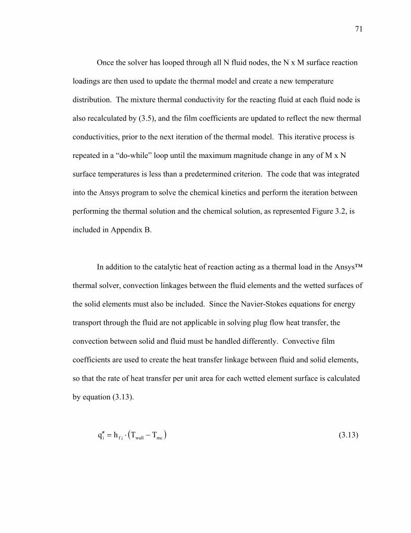
71
Once the solver has looped through all N fluid nodes, the N x M surface reaction
loadings are then used to update the thermal model and create a new temperature
distribution. The mixture thermal conductivity for the reacting fluid at each fluid node is
also recalculated by (3.5), and the film coefficients are updated to reflect the new thermal
conductivities, prior to the next iteration of the thermal model. This iterative process is
repeated in a “do-while” loop until the maximum magnitude change in any of M x N
surface temperatures is less than a predetermined criterion. The code that was integrated
into the Ansys program to solve the chemical kinetics and perform the iteration between
performing the thermal solution and the chemical solution, as represented Figure 3.2, is
included in Appendix B.
In addition to the catalytic heat of reaction acting as a thermal load in the Ansys™
thermal solver, convection linkages between the fluid elements and the wetted surfaces of
the solid elements must also be included. Since the Navier-Stokes equations for energy
transport through the fluid are not applicable in solving plug flow heat transfer, the
convection between solid and fluid must be handled differently. Convective film
coefficients are used to create the heat transfer linkage between fluid and solid elements,
so that the rate of heat transfer per unit area for each wetted element surface is calculated
by equation (3.13).
( mcwallifi TThq −⋅=′′ ) (3.13)

72
For some well-known geometries (flow through a round pipe, for example),
empirical correlations in the form of Nusselt vs. Reynolds numbers may be readily
available in the literature, and can be used to calculate the required film coefficients. In
some cases it may be necessary to experimentally determine the necessary correlations,
or to use computational models (computation fluid dynamics, or CFD, for example) to
solve the Navier-Stokes energy equations for a comparable geometry and flow regime to
calculate the film coefficients.
Throughout the chemically reacting region the flow composition changes
dramatically, and consequently the fluid properties can vary substantially over that
region. In order to account for this effect, the film coefficients in the reacting region are
updated to reflect the updated fluid compositions between iterations of the thermal solver
and chemical solver loop.
3.3 Detailed Description Of the Experimental Test Unit
An experimental unit was constructed and tested in order to validate the efficacy
of the developed modeling approach. An annular style reactor/heat exchanger was
selected, with the reacting flow passing through the outermost annulus so that the flow
temperature and composition could be easily measured at several points along the length
of the reacting region. The experimental unit can be seen in Figure 3.3.
The test unit was constructed so that the reactants pass through the reactor in a
counter-flow orientation to a hot air flow that serves as the heat source for the

73
endothermic reaction, with the air flowing through an annular flow channel immediately
adjacent the reacting flow channel. The reacting gas passage was located just inside the
outer shell, so that in-situ measurement of the reacting flow temperature and composition
would be possible without requiring thermocouples and gas sampling probes to penetrate
walls other than the outer shell.
Figure 3.3 – Integrated reactor/heat exchanger test unit
Thermocouple ports were located along the catalyst coated region length at five
axial positions, with the first immediately upstream of the coated region and the last

74
immediately downstream. Two ports were provided at each of the three intermediate
axial locations, spaced 180° apart, in order to provide some insight into any temperature
maldistribution that may occur in the angular direction. The first and last axial locations
had four ports each, spaced 90° apart, in order to provide better resolution of the angular
temperature profile.
Gas sampling ports were also provided at the 25%, 50% and 75% axial length
locations along the reacting zone, as close as possible to the thermocouple ports. These
sampling ports enable a small sample of the reacting gas to be extracted from the reactor
during operation, so that the composition of the flow can be determined. No ports were
included for the inlet and outlet gas composition, since gas samples can easily be drawn
from the plumbing upstream and downstream of the test unit and the composition is not
expected to change outside of the reacting region.
The test unit was constructed of stainless steel and Inconel alloys, with the
catalyst coated fin formed from FeCrAlloy®, an iron-chromium-aluminum alloy that is
especially suited for coating with an alumina washcoat. The FeCrAlloy® fin and a
conventional alloy fin for the heated air were nickel brazed onto a cylinder in order to
provide good thermal conductivity between the heat transfer surfaces. Following the
brazing operation, the outer FeCrAlloy® fin and the outer surface of the cylinder in the
fin region were catalyzed using a dip coating process. The finned cylinder after the dip
coating process is shown in Figure 3.4.

75
Figure 3.4 – Cylinder with brazed on and catalyzed fin structure
The section view of the test unit in Figure 3.5 shows the finned surfaces and the
measurement ports, with the blue fin being the catalyst-coated fin. The reformer
reactants enter the test unit through tube A, pass through the coated fin, and exit as the
reaction products through tube B. The heated air enters the test unit through the axial
inlet pipe C, and passes through an internal conduit (shown as dashed lines in Figure 3.5).
The heated air flows back through the red fin, and exits the test unit through the pipe D.

76
Figure 3.5 – Sectioned view of the integrated reactor/heat exchanger test unit
Diameters and wall thicknesses of the cylinders used to construct the test unit are
shown in Table 3.2. The finned reaction region extended over a length of 140mm, and
was located 115mm offset from the centerline of the reactant inlet pipe. The centerline
spacing between the reactant inlet pipe and product outlet pipe was 305mm. The catalyst
coated fin (shown in blue in Figure 3.5) was constructed of 0.15mm thick FeCrAlloy®
material corrugated into a 4.45mm high convoluted fin, with the individual fins spaced to
a fin pitch of 1.1mm (center to center distance). The hot air fin (shown in red in Figure
3.5) was constructed of 0.15mm thick UNS S31008 stainless steel material. The air fin
material was corrugated to a fin height of 6.43mm, with a fin pitch of 1.3mm. Prior to

77
reaching the catalyst-coated fins, the reactants pass through a 64mm long annular flow
channel formed between the outer shell cylinder and the extension of the reactor cylinder.
The total length of the outer shell cylinder was 343mm, with a 75mm long reactant inlet
plenum formed between the outer shell cylinder and the hot air outlet cylinder, and a
49mm long product exhaust plenum downstream of the reacting region.
Cylinder
outer diameter
wall thickness
reactor 82.6mm 1.24mm
outer shell 95.3mm 1.65mm
inner bounding cylinder for hot air fin 66.2mm 1.24mm
hot air inlet tube 25.4mm 1.65mm
hot air outlet tube 38.1mm 0.94mm
hot air outlet perpendicular stub 25.4mm 0.94mm
reactant inlet tube 12.7mm 0.94mm
product outlet tube 12.7mm 0.94mm
Table 3.2 – cylinder sizes used in the construction of the test unit.
The unit was tested in a reformer test stand, shown in Figures 3.6 – 3.9. The test
stand is covered with a Nabertherm Top Hat Kiln furnace hood to maintain a controlled
elevated ambient temperature around the test unit. The hood is capable of rising up to
allow access to the test unit. The test unit was mounted vertically so that all fluid
connections could be made from underneath. A 6kW Sylvania electric heater located
underneath the test stand (foil-wrapped cylinder in Figure 3.6) was used to heat the air
prior to it entering the test unit. The reactant stream was comprised of a mixture of steam
and methane, along with a small amount of inert nitrogen. The steam was generated from
de-ionized water, which was vaporized in a coil wrapped around the test unit exhaust
pipe underneath the furnace hood (indicated by the red arrow in Figure 3.8). The flow

78
rates of methane, water, nitrogen and air were controlled using mass flow controllers with
an accuracy of ±2%. After the liquid water was vaporized, the steam passed back out of
the hood area to mix with the methane so that the dry methane would not be exposed to
elevated temperature metal surfaces, in order to prevent coke formation.
The gas sampling ports were connected to high temperature needle valves (Figure
3.9) that could be manually adjusted to allow a sampling of gas from one of the ports to
be delivered to a gas chromatograph for compositional analysis. A Varian GC Series gas
chromatograph was used to measure the composition of the gas samples, with an
accuracy of ±1%. To measure the composition, a small sample of gas was drawn through
one of the needle valves at a rate of 200ml/min and was cooled to a dewpoint of
approximately 4°C. The dry gas was then delivered to the gas chromatograph.
Temperatures were measured using 1.5mm diameter K Type mineral insulated
thermocouples with stainless steel sheaths, from Omega. The thermocouples were
inserted into the fluid stream through Swagelok fittings that had been welded onto the test
unit. Temperature data was continuously collected using dedicated thermocouple
acquisition cards with cold junction correction. The accuracy for all temperature
measurements was ±2°C.

79
Figure 3.6 – Furnace test stand for testing of the integrated unit

80
Figure 3.7 – Integrated reactor/heat exchanger in the test stand
Figure 3.8 – Steam generator coil connected to the test unit

81
Figure 3.9 – Test unit mounted in the test stand, with gas sampling valves connected
The unit was tested with steam and methane at two different steam:carbon ratios.
For each of test case, stable operation was achieved and the unit was allowed to operate
with fixed flow rates and temperature control for a period of several hours, during which
time data was collected. In order to prevent carbon coke formation onto metal surfaces at
elevated temperatures, a minimum steam:carbon ratio of approximately 2.0 must be
maintained (Larminie & Dicks, 2000). Consequently, the lower limit of steam:carbon
ratio was set at 2.5 in order to ensure that coking of the test unit surfaces would not occur.
Operation at high steam:carbon ratios is limited as well, due to the increased amount of
heat necessary to generate the steam from liquid water. Using the test stand coiled tube
82
vaporizer to produce steam, the ability to achieve stable operation at higher steam:carbon
ratios was limited to a higher limit of 3.0. Test data was collected for steam:carbon ratios
of 2.5 and 3.0, with GHSV (volumetric flow rate through the reactor divided by the
reactor volume) of 4650 hr-1 and 5300 hr-1, respectively.
3.4 Description of the Computational Model
The experimental unit was modeled in Ansys™ following the methodology
described in section 3.2. In order to make the problem more tractable, the chemical
reaction section was modeled using a detailed sub-model with boundary conditions
mapped back and forth between the reactor sub-model and a thermal model of the full
heat exchanger.
The mesh of the full heat exchanger is shown in Figure 3.10 (only half of the
mesh is shown in order to expose the inner details). A total of 86,860 nodes were used to
construct the mesh, with temperature solved at each nodal location. Of the total nodes,
218 nodes were used to represent the plug flow hot air, while 188 nodes were used to
represent the plug flow reacting fluid. Additionally, one node was used to represent the
ambient temperature inside of the furnace hood. Convective heat transport between the
nodes for each of the two fluid streams was incorporated using FLUID116 type elements.
The solid geometry was meshed using SOLID70 elements, providing a linear temperature
gradient between adjacent nodes of the solid elements. SURF152 surface effect elements
were used to enable convective film coefficient heat transfer between the wetted surfaces

83
of the solid elements and the fluid nodes, as well as between the outer surfaces of the test
unit and the furnace ambient node.
Figure 3.10 – Sectional view of the finite element mesh in the full model
Film coefficients were determined using literature correlations for those sections
of the model where the fluid travels through a round cylinder, or in a plain annular
channel between two cylinders. Literature correlations were also used for the free
convection heat transfer from the outer surfaces of the test unit. Literature correlations
are not available, however, in the finned cylinder region of the model. As this is the
region where the majority of the heat transfer is expected to occur, using appropriate film
coefficients in this region is of high importance. Some development work on producing

84
heat exchangers of similar construction, with convoluted fin structures bonded to
cylindrical surfaces, has been performed by Modine Manufacturing Company of Racine,
Wisconsin, a commercial heat exchanger manufacturer. This unpublished work has
resulted in a CFD-based method of determining appropriate film coefficients for such
surfaces with boundary conditions that suitably represent counterflow heat exchange.
This method, which is described in detail in Appendix A, was used to provide film
coefficients for the finned cylinder surfaces. The fin geometry was not explicitly
included in the mesh of the full model. Instead, a film coefficient that includes the
efficiency of the fins was applied onto that portion of the plain cylinder surface that
corresponds to the finned region.
The film coefficients themselves are dependant on the thermal conductivity of the
fluids. With the exception of the reacting fluid as it passes through the catalyzed region
of the test unit, the thermal conductivity of the fluids was held to be constant. The
Nusselt numbers, hydraulic diameters, fluid thermal conductivity and resulting film
coefficients used in the various regions of the full model are listed in Table 3.3.

85
region Nu Dh
[mm] λfluid
[W/mK] h
[W/m2K] inner wall of reactant inlet tube 4.36(1) 10.8 0.08 32.3 inner wall of outer shell at reactant inlet plenum 7(2) 53.9 0.08 10.4
outer wall of hot air exit tube at reactant inlet plenum 10(3) 53.9 0.08 14.8
inner wall of outer shell in annular channel upstream of catalyzed fins 8(2) 9.4 0.08 68.1
outer wall of reactor cylinder in annular channel upstream of catalyzed fins 8(3) 9.4 0.08 68.1
inner wall of outer shell in the finned region 4.1(4) 1.6 varies varies inner wall of outer shell in annular channel downstream of catalyzed fins 8(2) 9.4 0.22 187.2
outer wall of reactor cylinder in annular channel downstream of catalyzed fins 8(3) 9.4 0.22 187.2
inner wall of outer shell at product outlet plenum 4.36(1) 92.0 0.22 10.4
inner wall of product outlet tube 4.36(1) 10.8 0.22 88.9 inner wall of hot air inlet tube 4.36(1) 22.1 0.06 11.8 inner wall of bounding cylinder for hot air fins 4.36(1) 63.72 0.06 4.1 inner wall of reactor cylinder in annular channel up and downstream of hot air fins 8(2) 13.9 0.06 34.5
outer wall of bounding cylinder in annular channel up and downstream of hot air fins 8(3) 13.9 0.06 34.5
inner wall of reactor cylinder in channel between reactor cylinder and hot air inlet tube 7(2) 54.7 0.06 7.7
outer wall of bounding cylinder for hot air fins in the finned region 4.4(4) 2.3 0.06 114.8
inner wall of reactor cylinder in the finned region 4.4(4) 2.3 0.06 746.2(5)
outer wall of hot air inlet tube in channel between reactor cylinder and hot air inlet tube 11(3) 54.7 0.06 12.1
inner wall of hot air exit tube in channel between hot air exit tube and hot air inlet tube 7(2) 43.9 0.06 9.6
outer wall of hot air inlet tube in channel between hot air exit tube and hot air inlet tube 10(3) 43.9 0.06 13.7
Table 3.3 – Internal heat transfer coefficients used in the full FEA model (1) fully developed laminar flow in a round duct, constant heat flux boundary condition (Kakaç, Shah, & Aung, 1987) (2) Figure 3.11, line Nuo
(2b)
(3) Figure 3.11, line Nui(2b)
(4) calculated by the method described in Appendix A (5) scaled by fin efficiency factor ε (equation A.10 in Appendix A)

86
Figure 3.11- Fully developed Nusselt numbers for constant heat flux at both walls in annular duct flow (Kakaç et al., 1987)
Heat transfer by free convection between the cylindrical external surfaces of the
test unit outer shell and the air inside the furnace hood was included through the
application of a free convection film coefficient. The film coefficient was applied as a
temperature-dependant term that varied locally with the film temperature (arithmetic
mean of the furnace internal ambient temperature and the local surface temperature). The
Rayleigh number for air over a range of film temperatures was calculated, using the outer
shell length as the characteristic length. Nusselt numbers were next calculated over the
range of film temperatures, using the correlation of equation 3.14 from Churchill and Chu
(1975a). This Nusselt correlation was stated by Incropera and DeWitt (1981) to be
appropriate for laminar free convection from vertical cylinders having a diameter
substantially larger than the boundary layer thickness. Prandtl number for air was
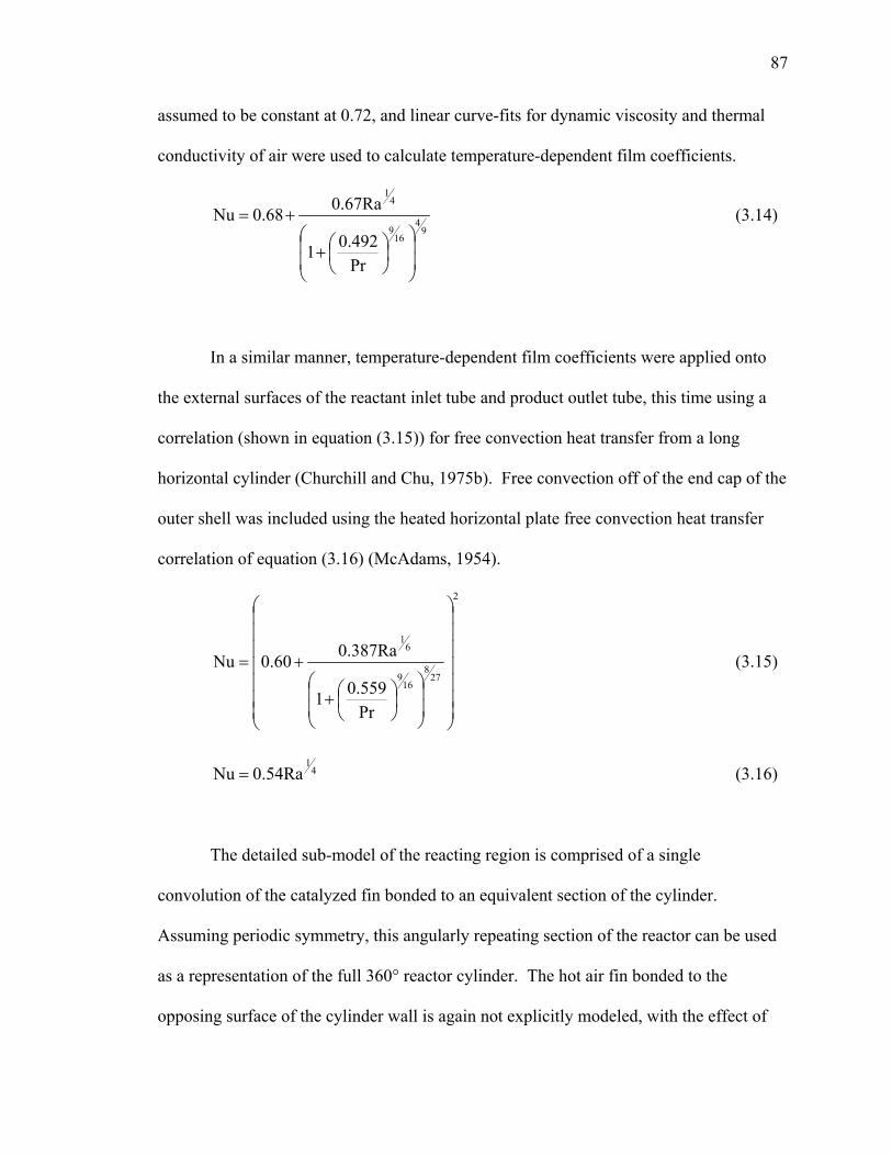
87
assumed to be constant at 0.72, and linear curve-fits for dynamic viscosity and thermal
conductivity of air were used to calculate temperature-dependent film coefficients.
94
169
41
Pr0.4921
0.67Ra0.68Nu
⎟⎟
⎠
⎞
⎜⎜
⎝
⎛⎟⎠⎞
⎜⎝⎛+
+= (3.14)
In a similar manner, temperature-dependent film coefficients were applied onto
the external surfaces of the reactant inlet tube and product outlet tube, this time using a
correlation (shown in equation (3.15)) for free convection heat transfer from a long
horizontal cylinder (Churchill and Chu, 1975b). Free convection off of the end cap of the
outer shell was included using the heated horizontal plate free convection heat transfer
correlation of equation (3.16) (McAdams, 1954).
2
278
169
61
Pr0.5591
0.387Ra0.60Nu
⎟⎟⎟⎟⎟⎟⎟
⎠
⎞
⎜⎜⎜⎜⎜⎜⎜
⎝
⎛
⎟⎟
⎠
⎞
⎜⎜
⎝
⎛⎟⎠⎞
⎜⎝⎛+
+= (3.15)
41
0.54RaNu = (3.16)
The detailed sub-model of the reacting region is comprised of a single
convolution of the catalyzed fin bonded to an equivalent section of the cylinder.
Assuming periodic symmetry, this angularly repeating section of the reactor can be used
as a representation of the full 360° reactor cylinder. The hot air fin bonded to the
opposing surface of the cylinder wall is again not explicitly modeled, with the effect of

88
the fin instead taken into account through the inclusion of the fin efficiency factor in the
heat transfer coefficient. This simplifies the mesh, as well as enabling the periodic
symmetry to be based exclusively on the catalyzed fin even when the hot air fin has a
different fin pitch. The relevant portions of the cylinders bounding the flows through the
reactor cylinder are included in the mesh of the sub-model, shown in Figure 3.12. The
mesh is constructed of 40,403 nodes, and uses the same element types as were used in the
full model. An additional layer of SURF152 surface effect elements are applied onto
those surfaces of the solid elements that would be coated with the catalyst washcoat. The
endothermic heat of reaction that is calculated for each of these elements in the chemical
solution section of the code is applied to the surface effect element as a negative heat
generation load for the thermal solution.

89
Figure 3.12 - Finite element mesh of the reactor submodel
The full reacting region length was discretized into 200 sections, each of which
includes a single fluid node to represent the reacting flow temperature and composition.
The catalyzed surface in each of the 200 sections was discretized into 71 separate catalyst
surface elements, so that the total number of catalyst surface elements was 14,200.
Temperature profiles are mapped to the bounding cylinders from the full model,
and function as boundary conditions for the thermal solution of the sub-model. In
addition, the temperatures of the reacting flow and the hot air flow entering the reactor

90
section are taken from the full model. Film coefficients for the hot air side are same as
those used in the full model, and are listed in Table 3.3. The Nusselt number for the
reacting side flow channels was calculated to be 4.1 using the method described in
Appendix B, with a corresponding hydraulic diameter of 1.6mm. The film coefficient
will vary, though, over the length of the reacting region due to the dramatic change in
fluid composition. In order to account for this, the mixture fluid properties are
recalculated at every position along the reacting fluid flow path after the composition is
calculated in the chemical solution stage, and the resultant film coefficients are calculated
for use in the following iteration of the thermal solver.
Once the reactor sub-model has a converged solution for the given boundary
conditions, the temperature profile of the reactor cylinder is mapped to the full model,
along with the reacting fluid temperatures and the film coefficients in the reacting region.
The mapped fluid temperatures and film coefficients in the reactor region of the full
model are used to calculate a new temperature profile on the bounding cylinder
surrounding the reacting zone in the full model. The hot air temperatures and the
temperature profile on the bounding cylinder surrounded by the reacting zone are also
solved within the full model by calculating the convective heat transfer to the
temperature-mapped reactor cylinder, as well as the heat transfer through the bounding
wall to the exhaust flow upstream of the reacting zone. Once the full model is solved, the
resulting bounding cylinder temperatures in the reacting zone are mapped back to the
reactor sub-model, along with the reactant and hot air inlet temperatures to the reacting

91
zone. The sub-model and full model sequential solution process is repeated until the
mapped boundary conditions no longer change.
As mentioned in section 3.2, an effectiveness factor that accounts for the
diffusional resistances and the difference in intrinsic catalytic activity between the
precious metal catalyst and the nickel catalyst of Xu and Froment (1989a) must be
determined. To accomplish this, a sample of the reacting flow fin structure was brazed to
a flat plate and catalyzed using the same washcoat process used for the reactor cylinder.
This flat plate sample, shown in Figure 3.13, measured 60mm wide by 60mm long. The
sample was placed into a furnace and kept at a controlled temperature while a mixture of
steam and methane was flowed through the sample. The flow rate of steam and methane
was gradually increased while the exit composition was monitored with a gas
chromatograph.
By increasing the GHSV until the exit composition begins to deviate from
equilibrium, the effectiveness factor can be empirically determined using equation 3.11.
In order to use this equation the catalyst bed density ρB, defined as the mass of catalyst
used per unit volume of the reactor, must be known. This number is considered to be
proprietary to the catalyst suppliers. The exact value, however, does not need to be
known so long as the catalyst loading is the same between the calibration test sample and
the actual reactor, since any deviation from the exact value will be taken into account in
the effectiveness factor η. A value of 3 grams of catalyst per liter was used as the bed
density.

92
The kinetic portion of the reactor model was solved at a constant temperature
corresponding to the temperature at which the furnace is maintained. Since the reaction
proceeds isothermally, the model is able to converge very quickly. The model was run
with a range of effectiveness factors and the GHSV was varied over the same range as
was used in the sample testing. By comparing the GHSV at which the predicted exit
composition begins to deviate from equilibrium with the GHSV at which the sample exit
composition begins to deviate from equilibrium, the appropriate effectiveness factor can
be determined. The effectiveness factor determination was performed at several
temperatures in order to ensure that the empirical factor did not have a significant
temperature dependency.
Figure 3.13 – Reaction rate calibration isothermal test sample

93
3.5 Design Optimization Study
In order for the modeling approach to have utility in reactor design applications, it
should be able to be used as a tool to evaluate various design options. This would then
allow reactor designers to optimize the design in order to provide a target level of
performance at a minimum component cost or size. To that end, in addition to validating
the model results with empirical data, the sensitivity of the integrated reactor/heat
exchanger design to variations in the physical attributes of the reactor section was
investigated.
The computational model was subjected to a series of computational runs
comprising a 24-1 fractional factorial study. In a factorial design of experiments, the
effects that two or more factors have on the results of an experiment (or calculation) can
be separated out from one another in order to evaluate the individual contribution of each
factor (Montgomery, 1997). In a 24-1 fractional factorial matrix, four variables are
considered, each having two possible values, in a total of eight combinations. The eight
combinations (or computational runs) are selected from the sixteen possible combinations
of the variables in such a way that the effects of each factor in isolation can still be
determined. By reducing the number of runs by half, the interaction effects between
three variables become confounded with the main effects due to aliasing. However, the
main effects are typically significantly greater than the interaction effects, especially the
three-factor interactions, and for a general screening study this confounding should not be
of great significance(Montgomery, 1997).

94
The four factors that were varied over the runs are all parameters of the extended
surfaces to which the catalyst is applied. One factor, the thickness of the fin material,
would affect only the rate at which heat can be transported to the catalyst sites at the ends
of the fins. This factor would not affect either the GHSV or the catalyzed surface area.
A second factor, the fin pitch of the catalyzed fins, can directly increase or decrease the
surface area available for both chemical reaction and heat transfer to and from the
reacting flow. The Nusselt number was assumed to not vary with the change in channel
aspect ratio due to varying the fin density. This factor does not change the GHSV, since
the reactor volume in that calculation is based on the full volume of the annulus including
both free-flow volume and the solid volume of the catalyst substrate. The third and
fourth factors are the height of the catalyzed fins, and the length of the reacting region.
These two factors both directly influence both the GHSV and the available surface area.
High and low values were chosen for all four of the factors, as shown in Table
3.4. The values were selected so that the high value for each factor was approximately
112% of the low value. In this way, the influence effect that is calculated for each factor
corresponds to the influence of a 12% change in that factor.
FACTOR low
value high value
fin height [mm] 4.45 4.98 fin thickness [mm] 0.152 0.17 reactor length [mm] 125 140 fin pitch [mm] 0.938 1.05
Table 3.4 – High and low limits for variables in factorial study

95
The geometry of the test unit was again used for the optimization study. The
lengths of the cylinders were kept unchanged, since the high value for the reactor length
was chosen to coincide with the length of the heat exchange/reaction region in the test
unit. For those cases where the reactor length was at the low value, the reactant inlet end
was kept the same and the catalyzed reactant fin and un-catalyzed hot air fin were
shortened from that end, so that a longer un-finned region of the cylinder was modeled at
the reacting flow outlet end. Similarly, the low value of the fin height was chosen to
coincide with the catalyzed fin height in the test unit. For those cases where the fin
height was at the high value, the diameter of the outer cylinder was increased by 1.06mm,
or twice the increase in fin height.
In order to properly evaluate the impacts of the individual factors on the
performance of the reactor/heat exchanger, the operating conditions must be such that the
reacting flow does not approach thermodynamic equilibrium. Consequently, the flow
rates of both the reacting flow and the hot air flow were doubled from their values in the
test unit validation testing. This effectively doubles the nominal GHSV, which should
result in the reaction products achieving a rate of conversion that is substantially lower
than what would be dictated by equilibrium. In this way, the impacts of the factor
variations should be observable.
The 24-1 factional factorial test matrix is shown in Table 3.5. In this test matrix
the main effects of each of the variables is aliased with the three-factor interaction effects
of the other variables. The eight conditions were modeled and solved in the same manner

96
as was done for the validation of the experimental unit. The methane conversion (the
percentage of the incoming methane that is consumed by the reactions) was recorded as
the output variable for each run, and the contributing effect of the variation of each
individual factor was analyzed.
fin thickness fin height
reactor length fin pitch
1 low low low low 2 high low low high 3 low high low high 4 high high low low 5 low low high high 6 high low high low 7 low high high low
Run
No.
8 high high high high Table 3.5 – Fractional factorial test matrix

97
4. RESULTS
4.1 Experimental Unit Test Results
Due to control issues associated with the water flow rate control system, only a
limited amount of useful test data was able to be recorded with the experimental unit.
Since the gas chromatograph was only able to measure the composition from one of the
flow taps at a time, it was necessary to maintain stable and consistent operation over a
period of hours in order to ensure that all of the data was being collected at the same
operating condition. Two test conditions were able to provide data over a stable long-
term operation of several hours. These two conditions were at steam:carbon (S:C) ratios
of 2.5 and 3.0. Table 4.1 lists the operating conditions for the two test cases. These
conditions were used as inputs to the comparative computational models. The absolute
pressure in the steam reformer, required for the kinetic calculations, was assumed to be
equal to the gage pressure of reactants into the test unit added to 1.01 bar. The testing
was performed about 28 miles south of London, England, in the vicinity of Gatwick
airport, which has an elevation above sea level of approximately 200 feet.
S:C =2.5 S:C=3.0 accuracy water flow rate 123 mg/s 148 mg/s ± 2% methane flow rate 3.69 slm 3.69 slm ± 2% nitrogen flow rate 0.155 slm 0.155 slm ± 2% hot air flow rate 280 slm 280 slm ± 2% temperature of hot air into test unit 674.5°C 674.3°C ± 2°C temperature of reactants into test unit 414.5°C 402.9°C ± 2°C temperature of furnace ambient 419.2°C 418.5°C ± 2°C gage pressure of reactants into test unit 80.5 mbar 91.7 mbar ± 2 mbar
Table 4.1 – operating conditions for the two test cases
In the first run, at a molar S:C ratio of 2.5, stable, steady-state operation was
maintained for a period of 5.5 hours, during which time temperature data was recorded

98
from the thermocouples inserted into the reactant flow stream through the outer wall of
the reactor. Stainless steel sheathed Type K thermocouples with a diameter of 1.5mm
were used to measure the fluid temperatures. Tise thermocouple diameter is comparable
to the the channel width between adjacent fin legs (approximately 1mm). In order to
ensure that the thermocouple does not make incidental contact with the fin itself, and to
avoid blocking of the flow through the channel, the thermocouple depth of insertion was
set so that the tip of the thermocouple extended just beyond the inner wall of the outer
shell cylinder. Figure 4.1 shows the recorded temperature data over the 5.5 hour
timeframe.
540
560
580
600
620
640
660
680
14:00 15:03 16:06 16:52 17:31 18:28 19:24
Time of Data Recording
Tem
pera
ture
[°C
]
reactor inlet (0°, 90°, 180°, 270° angular position)
25% of reactor length
270° position
90° position
50% of reactor length (90°, 270° position)
75% of reactor length (90°, 270° position)
reactor exit
90°, 180° position 0°, 270° position
Figure 4.1 – Experimental temperature data for flow through the reacting side, plotted as a function of time, S:C=2.5

99
The graphed data shows a fairly constant temperature profile over the time period
that data was recorded. Very little angular variation of temperatures was observed,
although the temperatures at the exit of the reacting region did show about 5°C higher
temperature in one half than in the other half. At 25% of the reactor length a
circumferential temperature variation was observed for the first three hours, but this
variation disappeared over the last 2.5 hours. The temperatures appear to rapidly increase
in the first 75% of the reactor, with the rate of increase slowing down considerably over
the last 25%. Overall, the temperature distribution appears to be stable over time and
uniform over the circumference.
The composition of the reacting flow was measured with a gas chromatograph
over the same 5.5 hour time period during which the temperature data was collected.
Each collection port was sampled for a period of time in order to collect the composition
data. The gas chromatograph requires that the sample be cooled down to room
temperature, and that any moisture is removed. Relative concentration of the different
species (except for H2O, which has been condensed out) is measured by the gas
chromatograph. Since the flow rate of the inert nitrogen (N2) should remain unchanged
through the reactor and is known, the relative concentrations can be converted to a molar
flow rate through the entire reactor cross-section. The molar flow rate of H2O can be
calculated by evaluating the oxygen imbalance in the resulting molar flow rates.
The molar flow rate data for the 2.5 S:C case is shown in Figure 4.2, along with
the time-averaged temperature data at each location. As can be seen in the plot, the
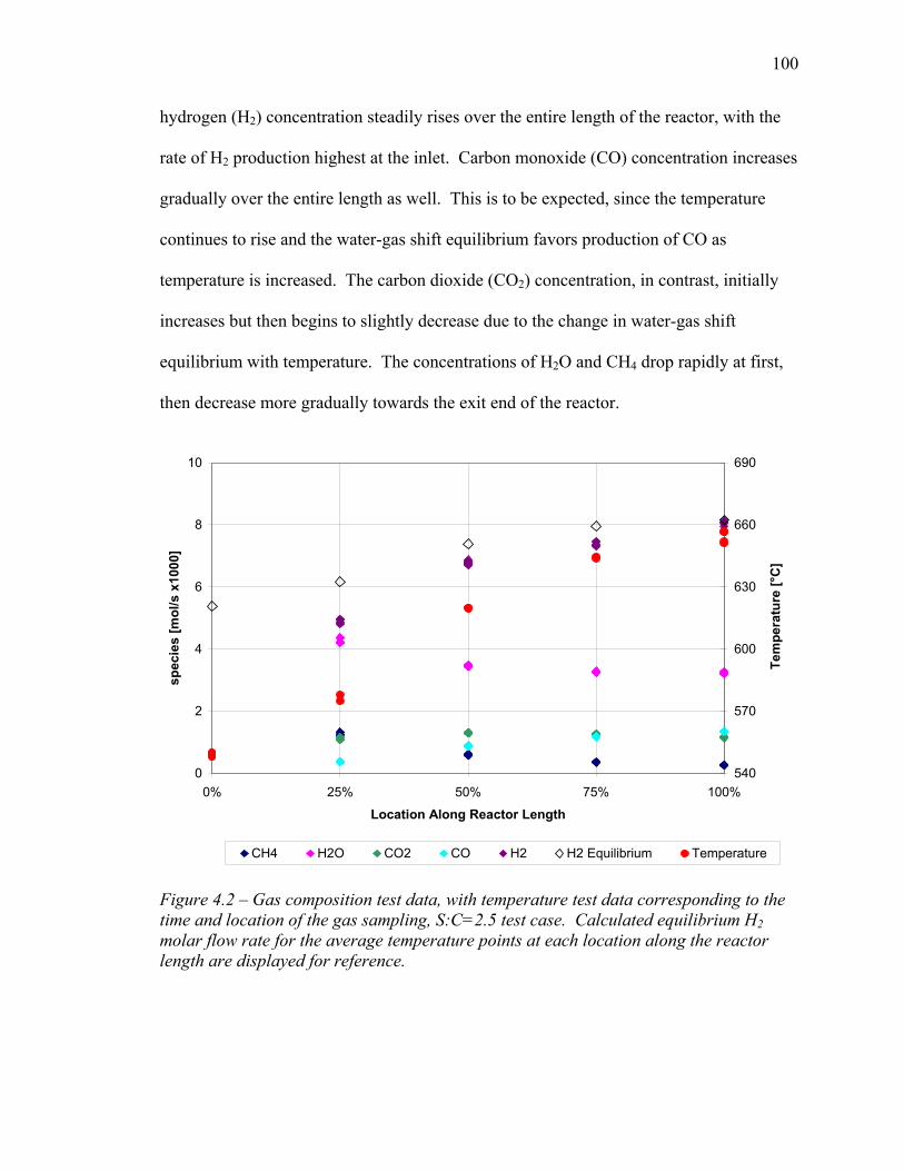
100
hydrogen (H2) concentration steadily rises over the entire length of the reactor, with the
rate of H2 production highest at the inlet. Carbon monoxide (CO) concentration increases
gradually over the entire length as well. This is to be expected, since the temperature
continues to rise and the water-gas shift equilibrium favors production of CO as
temperature is increased. The carbon dioxide (CO2) concentration, in contrast, initially
increases but then begins to slightly decrease due to the change in water-gas shift
equilibrium with temperature. The concentrations of H2O and CH4 drop rapidly at first,
then decrease more gradually towards the exit end of the reactor.
0
2
4
6
8
10
0% 25% 50% 75% 100%
Location Along Reactor Length
spec
ies
[mol
/s x
1000
]
540
570
600
630
660
690
Tem
pera
ture
[°C
]
CH4 H2O CO2 CO H2 H2 Equilibrium Temperature
Figure 4.2 – Gas composition test data, with temperature test data corresponding to the time and location of the gas sampling, S:C=2.5 test case. Calculated equilibrium H2 molar flow rate for the average temperature points at each location along the reactor length are displayed for reference.

101
In the second run where data was recorded, the steam flow rate was increased to
provide a S:C ratio of 3.0. For this run, the data was recorded over a period of 2.5 hours.
In general, the results were very similar to those observed in the first run. The
temperature data over the 2.5 hours is shown in Figure 4.3. Again, the temperatures
appear to be relatively constant with respect to time. As was the case in the first run, the
temperatures at the reactor exit show a variation of approximately 5°C from one half of
the reactor to the other half. In this run the temperatures at 25% of the length also show a
deviation of as much as 5°C. The temperature profile over the reactor length appears
very similar to the profile seen in the first run.
540
560
580
600
620
640
660
680
14:29 15:10 15:55 16:42 16:51
Time of Data Recording
Tem
pera
ture
[°C
]
reactor inlet (0°, 90°, 180°, 270° angular position)
25% of reactor length
270° position
90° position
50% of reactor length (90°, 270° position)
75% of reactor length (90°, 270° position)
reactor exit
90°, 180° position 0°, 270° position
Figure 4.3 – Experimental temperature data for flow through the reacting side, plotted as a function of time, S:C=3

102
The composition of the reacting flow was also measured for the 3.0 steam:carbon
ratio run, again using the gas chromatograph. The resulting molar flow rates at each of
the sampling locations are shown in Figure 4.4. The composition results are very
comparable to those of the first run.
0
2
4
6
8
10
0% 25% 50% 75% 100%
Location Along Reactor Length
spec
ies
[mol
/s x
1000
]
540
570
600
630
660
690
Tem
pera
ture
[°C
]
CH4 H2O CO2 CO H2 H2 Equilibrium Temperature
Figure 4.4 – Gas composition test data, with temperature test data corresponding to the time and location of the gas sampling, S:C=3. Calculated equilibrium H2 molar flow rate for the average temperature points at each location along the reactor length are displayed for reference.
A check was performed on the compositional data to verify that the elemental
carbon, hydrogen and oxygen were conserved. At each data point the molar flows of
these elements was compared to the known incoming molar flows. The results are
displayed graphically in Figures 4.5 and 4.6. It was found that there was some lack of
conservation. As shown in the figures, the flow of hydrogen atoms appears to be as much

103
as 8% lower than expected for both runs. Conversely, the carbon and oxygen elemental
flow rates appear to be around 1% higher than expected. In all cases the error in carbon
flow is exactly equal to the error in oxygen flow, since the water content of the samples is
calculated from the carbon-containing species flow rates so that the known
oxygen:carbon ratio is maintained.
-10.0%
-8.0%
-6.0%
-4.0%
-2.0%
0.0%
2.0%
0% 25% 50% 75% 100%
Location Along Reactor Length
erro
r rel
ativ
e to
inle
t flo
w
C H O
Figure 4.5 – Element conservation error in test data, S:C=2.5.

104
-10.0%
-8.0%
-6.0%
-4.0%
-2.0%
0.0%
2.0%
0% 25% 50% 75% 100%
Location Along Reactor Length
erro
r rel
ativ
e to
inle
t flo
w
C H O
Figure 4.6 – Element conservation error in test data, S:C=3
The observed elemental imbalance could be caused by the true S:C ratio being
different from the ratio that was thought to be present. In order for this to be the case, the
true S:C ratio would have to be both less than the value that was thought to be present,
and fluctuating. For the 2.5 S:C run, the elemental imbalance would be reduced to zero
percent at each data sampling point if the actual steam:carbon varied over a range of
2.05-2.30. This amount of error in the mass flow rates is, however, unlikely. An
alternative explanation for the lack of element balance is that the H2 content was under-
sampled by the gas chromatograph. The amount of under-sampling that would be
required to produce the observed results would range from approximately 7-15%.

105
4.2 Reaction Calibration Sample Test Results
The reaction calibration test sample was tested at varying Gas Hourly Space
Velocities (GHSV) at 600°C, 650°C and 700°C. The targeted steam:carbon ratio was
2.5, but the water flow control was not able to maintain that ratio exactly. Over the
course of the data collection, the actual S:C ratio was varied from 2.3 to 2.5. The GHSV
was increased from 3000 hr-1 to 15,000 hr-1 in increments of 2000 hr-1. Above
approximately 15,000 hr-1 the steam generator did not have sufficient capacity to produce
steam at the required flow rates.
The CH4 conversion for each of the runs is graphed in Figure 4.7. Unfortunately
the GHSV was never high enough to cause the CH4 conversion to drop significantly
below the equilibrium conversion level. At low GHSV values (3000 hr-1 to 7000 hr-1) the
CH4 conversion is slightly greater than it is at the higher GHSV values, due to the
presence of a constant flow rate of N2. At low GHSV values the flow rate of CH4 and
H2O is significantly reduced while the flow rate of N2 is kept constant, so that the partial
pressures of the reacting species is quite a bit lower than at the higher GHSV runs. The
resulting low pressure operation drives up the equilibrium level of CH4 conversion.

106
50%
60%
70%
80%
90%
100%
1000 3000 5000 7000 9000 11000 13000 15000 17000
GHSV [hr-1]
CH
4 Con
vers
ion
600°C 650°C 700°C
Figure 4.7 – Methane conversion results from isothermal kinetics calibration testing
The kinetic computational model was run isothermally for each of the cases
plotted in Figure 4.7. For each experimental run the temperature, GHSV, S:C ratio, and
N2 flow rate was matched to the test data and the computational model was run with three
different values for catalyst effectiveness (η=3, 9 and 15). The computational results are
compared with the experimental results in Figure 4.8.
With η=3, the computed methane conversion is significantly lower than the
experimentally obtained results for all cases, even at the highest temperatures. With η=9,
the computational model results for CH4 conversion matched the experimental results at
700°C but were still significantly lower at the reduced temperatures of 650°C and 600°C.

107
Only at η=15 were the reaction kinetics fast enough to have the computational model
results match the experimental results for all cases.
50%
60%
70%
80%
90%
100%
50% 60% 70% 80% 90% 100%
CH4 conversion - experiment
CH
4 con
vers
ion
- com
puta
tion
η = 3 η = 9 η = 15
Figure 4.8 – Correlation between calibration test runs and catalyst effectiveness factor
Unfortunately, since the GHSV was never increased to a high enough level to
have the CH4 conversion deviate substantially from equilibrium, it is impossible to tell if
η=15 is high enough. Given the available data, 15 was assumed to be an appropriate
value of η for the catalyst and substrate geometry.
4.3 Computational Model Results
The computational model was run for both of the operating conditions at which
data was collected. The model was set to automatically iterate eight times between

108
solving the thermal/chemical submodel and solving the full geometry thermal model.
After the eight iterations were completed, the results were evaluated in order to determine
whether or not the solution had converged. Convergence, in this case, can be determined
by evaluating the change in the boundary conditions that are mapped between solutions
of the two models. It was found that after the eight iterations the temperature boundary
conditions that were being mapped were no longer changing substantially, so the solution
was considered to be converged at that time. On a Dell Precision M90 laptop computer
with a 1.83 GHz Intel Core 2 Duo T5600 microprocessor and 4GB of RAM, the solution
time for each of the two cases was approximately three hours and forty minutes.
The temperature profile of the full model for the 2.50 steam:carbon case is shown
in Figure 4.9. As is to be expected, the steepest gradient can be seen in the area where
the finned heat exchange surfaces are located. The total range of temperatures is
approximately 270°C, ranging from low temperatures between 400° and 430°C at the
reactant inlet to high temperatures between 640°C and 670°C in those areas exposed only
to the hot air flow upstream of the finned region.

109
Figure 4.9 – temperature profile in the full finite element model, S:C=2.5
Figure 4.10 shows the temperature of the plug flow reacting fluid along the entire
flow path of the full test unit finite element model. The graph reveals that the fluid
increases in temperature fairly rapidly once it exits the inlet tube and enters into the main
body of the device, increasing by approximately 130°C before it reaches the entrance of
the reacting region. The fluid in this region would be heated by the hot air from the hot
air exit cylinder, while at the same time rejecting heat through the outer shell to the
furnace ambient. Through the reacting region the fluid is further heated by the hot air,
but downstream the fluid is cooled by heat loss to the furnace ambient.

110
400
450
500
550
600
650
700
0 100 200 300 400 500Location along reacting flow path [mm]
Tem
pera
ture
[°C
]
reactant inlet tube
reacting region
product outlet tube
Figure 4.10 – Temperature of the reacting fluid along the entire length of the flow path in the model of the full test unit, S:C=2.5
The temperature profile from the reactor sub-model for the same case is shown in
Figure 4.11. The reacting flow is moving in the +z-direction, while the hot air flow is
moving in the –z-direction. The range of temperatures over the catalyzed fins is similar
to the range of fluid temperatures in the reacting region seen in the graph of Figure 4.10.
However, unlike the plug flow fluid whose temperature varies in the z-direction only, the
surface temperatures show a distinct temperature gradient in the fin height direction over
a substantial portion of the flow length.

111
Figure 4.11 – Temperature profile over the catalyzed in and reactor cylinder, from the reactor submodel for the case of S:C=2.5
In order to better quantify the temperature profile along the fin height, the fin
surface temperatures were extracted at 25%, 50% and 75% of the reactor length. These
temperatures were then converted into temperature differentials from the local bulk fluid
temperature (a measure typically referred to as “θ” in heat transfer calculations). The
results are graphed in Figure 4.12. The temperature differential and the gradient both
decrease with distance along the reactor length. The greatest gradient, at 25% reactor
length, is approximately 12°C over the full fin height. This has decreased down to about
4°C at 75% of reactor length. Figure 4.12 additionally shows that (Tsurf-Tbulk) is negative
over as much as half of the fin height at the 25% and 50% reactor length locations. This
implies that those areas are actually being heated by the reacting flow due to conduction
heat transfer resistance in the fin limiting the ability to transfer heat from the hot air.

112
-4
-2
0
2
4
6
8
10
0 1 2 3 4 5
Distance from base of fin [mm]
(Tsu
rf - T
bulk) [
°C]
25% of reactor length 50% of reactor length 75% of reactor length
Figure 4.12 – differential temperature (surface minus bulk fluid) variation over the fin height at 25%, 50% and 75% reactor length, S:C=2.5
When the temperature profile over the catalyzed surface varies, the strongly
temperature-dependent reaction rates will also vary over the surface. In order to evaluate
the extent of this variation, the chemical reaction rate (expressed as the rate at which heat
is consumed by the overall endothermic chemical surface reactions per unit area) over the
catalyzed surface was plotted at the reactor inlet, midpoint and outlet. The plots are
shown in Figures 4.13-4.15, and reveal that the reaction rate varies at least as strongly in
the fin height direction as it does in the reactor length direction. As is to be expected, the
reaction rate overall decreases from the inlet to the outlet, with the reaction rate in the
first 10% of the length being 16-19 times as high as the reaction rate in the last 10% of
the length. Generally speaking, at all three locations the reaction rate at the fin crest is
approximately half the reaction rate at the base of the fin. These results strongly support

113
the presupposition that capturing the variation over the profile of the heat exchange
surfaces is vital to accurately modeling the performance of a process-intensified steam
methane reformer with catalyzed heat exchange surfaces. If a single value at each z-
location was used to represent the surface temperature and reaction rate, such a variation
would not be able to be captured.
Figure 4.13 – Surface reaction rate per unit area in first 10% of reactor length, S:C=2.5

114
Figure 4.14 – Surface reaction rate per unit area in middle 10% of reactor length, S:C=2.5
Figure 4.15 – Surface reaction rate per unit area in last 10% of reactor length, S:C=2.5

115
4.4 Comparison of Computational and Experimental Results
The temperature and composition of the reacting fluid flow as calculated in the
computational model was compared with the experimental results at the same operating
conditions. In Figure 4.16, the calculated temperature profile of both fluids at the 2.5 S:C
ratio is shown, along with the data from the thermocouples for that case. Immediately
evident from the graph is the counter-flow heat exchange nature of the reactor/heat
exchanger, with the air flow outlet temperature being significantly lower than the reacting
flow outlet temperature.
500
525
550
575
600
625
650
675
700
0% 25% 50% 75% 100%
Location Along Reactor Length
Tem
pera
ture
[°C
]
Reacting Flow Air Flow
Figure 4.16 – Comparison of computational and experimental fluid temperatures in the reacting region, S:C=2.5. Lines are computation results, circles are experiment results

116
Also evident is a very good overall agreement between the calculated reacting
flow temperature and the thermocouple measurements. It should be noted however that
the temperatures measured by the thermocouples are not exactly comparable to the
volumetrically-averaged temperatures computed by the software, since substantial
thermal gradients (x- and y-direction) could exist within the experiment, for example
towards the apex of the fins. In comparing the experimental and computed results it can
be seen that although the temperature of the reacting flow increases significantly from the
test unit inlet to the entrance of the reaction section, the calculated temperature at the
entrance almost exactly matches the measured temperature. In addition, the calculated
temperature profile over the length of the reactor matches very well with the measured
temperatures.
A similar comparison for the 3.0 S:C case is shown in Figure 4.17. Again, the
agreement between the calculations and the test data is quite good. For both cases the
inlet, 75% length, and outlet temperatures have the best agreement. At 25% of the length
the results show the least amount of agreement, with the calculated temperature being
approximately 15-20°C higher than the measured temperature. It is unclear whether this
is due to experimental error or error in the computational model.

117
500
525
550
575
600
625
650
675
700
0% 25% 50% 75% 100%
Location Along Reactor Length
Tem
pera
ture
[°C
]
Reacting Flow Air Flow
Figure 4.17 – Comparison of computational and experimental fluid temperatures in the reacting region, S:C=3. Lines are computation results, circles are experiment results
The ability of the model to accurately capture the overall heat transfer from the
hot air flow, including losses to the furnace ambient, was assessed by comparing the
measured hot air outlet temperature to the calculated value. In the 2.5 S:C case, the time-
averaged hot air outlet temperature was 598°C, whereas the model results gave a
temperature of 595°C. This very good agreement indicates that the net heat transfer was
indeed captured well. Similar results were observed for the 3.0 S:C case, where the
measured and calculated hot air outlet temperatures were 594°C and 591°C, respectively.
The calculated bulk fluid molar flow rate for each species along the reacting
region length was compared to the molar flow rates derived from the gas chromatograph

118
data. The comparison for the 2.5 S:C ratio is shown in Figure 4.18. Again, the
agreement between calculation and experimental measurement is quite strong. Very
good agreement is seen for H2O, CO, CO2, and CH4. The molar flow rate for H2,
however, appears to be over-predicted. Very steep gradients are seen in the computed
mole fractions with these probably due to the assumption of infinitely fast molecular
diffusion in the fluid domain.
0
2
4
6
8
10
0% 25% 50% 75% 100%
Location Along Reactor Length
spec
ies
[mol
/s x
1000
]
CH4 H2O CO2 CO H2
Figure 4.18 – Computational and experimental fluid composition, S:C=2.5. Lines are computation results, diamonds are experiment results
The discrepancy between calculated and measured hydrogen flow is not
unexpected, since the measured hydrogen flow rate was found to be low based on
conservation of elements. The experimental results were adjusted by increasing the H2
content until the element conservation error disappeared. The resulting flow rates were

119
then compared again to the calculated molar flow rates. The graph showing the adjusted
values is shown in Figure 4.19.
0
2
4
6
8
10
0% 25% 50% 75% 100%
Location Along Reactor Length
spec
ies
[mol
/s x
1000
]
CH4 H2O CO2 CO H2
Figure 4.19– Computational and adjusted experimental fluid composition, S:C=2.5. Lines are computation results, diamonds are adjusted experiment results
The adjusted flow rates for CH4, CO, CO2, and H2O still matched well with the
calculated flow rates. The adjusted H2 flow rate showed much better agreement with the
calculated results, with the calculated flow rate now slightly under-predicting the adjusted
experimental flow rate.
The comparison of the calculated molar flow rates of the 3.0 S:C case to the gas
chromatograph data is shown in Figure 4.20. The calculated flow rate for hydrogen
shows slightly greater deviation from the test data than was seen in the 2.5 S:C case. The
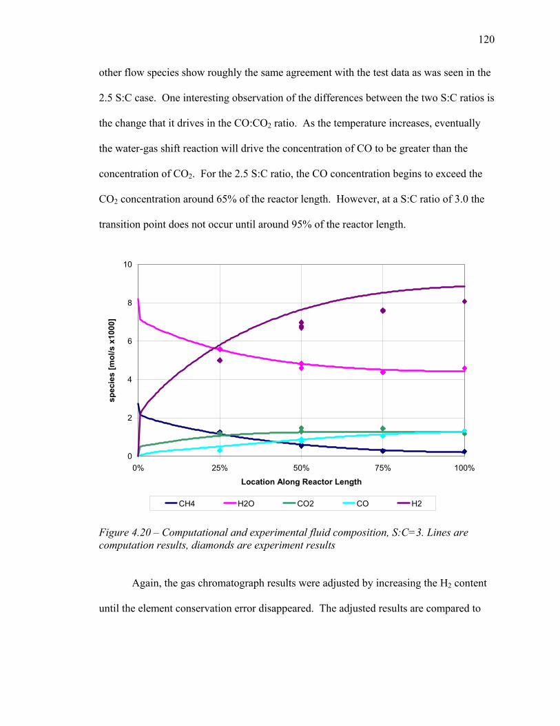
120
other flow species show roughly the same agreement with the test data as was seen in the
2.5 S:C case. One interesting observation of the differences between the two S:C ratios is
the change that it drives in the CO:CO2 ratio. As the temperature increases, eventually
the water-gas shift reaction will drive the concentration of CO to be greater than the
concentration of CO2. For the 2.5 S:C ratio, the CO concentration begins to exceed the
CO2 concentration around 65% of the reactor length. However, at a S:C ratio of 3.0 the
transition point does not occur until around 95% of the reactor length.
0
2
4
6
8
10
0% 25% 50% 75% 100%
Location Along Reactor Length
spec
ies
[mol
/s x
1000
]
CH4 H2O CO2 CO H2
Figure 4.20 – Computational and experimental fluid composition, S:C=3. Lines are computation results, diamonds are experiment results
Again, the gas chromatograph results were adjusted by increasing the H2 content
until the element conservation error disappeared. The adjusted results are compared to

121
the model results in Figure 4.21. As was the case for the 2.5 S:C ratio, the discrepancy in
the hydrogen concentration was substantially improved.
0
2
4
6
8
10
0% 25% 50% 75% 100%
Location Along Reactor Length
spec
ies
[mol
/s x
1000
]
CH4 H2O CO2 CO H2
Figure 4.21 – Computational and adjusted experimental fluid composition, S:C=3. Lines are computation results, diamonds are adjusted experiment results
The sensitivity of the model results to variation of some of the critical parameters
in the model was evaluated. The Nusselt numbers in the fin channels for the reacting
fluid and for the hot gas, as well as η, were each individually varied by +50% and -50%,
and the S:C=2.5 case was rerun for a total of six additional runs. CH4 conversion and
reacting flow temperature were selected as the two variables that would be used to assess
the sensitivity. The results are plotted along with the test data points in Figures 4.22 and
4.23. There appears to be no sensitivity to variation in the reacting flow Nusselt number.
This is not unexpected, since the sensible heating of the reacting flow is only a small

122
portion of the heat duty in the reactor. Substantially greater sensitivity to variations in the
other two parameters was observed. Overall, the baseline values showed the best match
to the test data. None of the model parameter changes was able to adequately indicate
resolutions to the discrepancies seen in the species concentrations or temperature
measurements.
The Nusselt number on the reacting flow side was developed using boundary
conditions for non-reacting heat transfer surfaces, whereas it is being used with reacting
surfaces in the computational model. These differences in boundary condition cast some
doubt on the appropriateness of this Nusselt numbers for this application. However, the
apparent insensitivity of the results to the magnitude of the Nusselt number on the
reacting flow side would suggest that non-reacting flow Nusselt numbers can be used for
SMR catalyst-coated surfaces without creating significant error.

123
Figure4.22- Sensitivity of methane conversion along reactor length to variation in η and Nusselt (S:C=2.5). Lines are computation results, diamonds are experiment results
Figure 4.23 – Sensitivity of reacting flow temperature along reactor length to variation in η and Nusselt (S:C=2.5). Lines are computation results, diamonds are experiment results

124
4.5 Factorial Study Results
The methane conversion at the reactor outlet for the eight runs in the fractional
factorial study was entered into a response table (Table 4.2) and the individual
contribution of each of the four variables was calculated. The average methane
conversion at the high level of each variable was compared to the average methane
conversion at the low level. The difference between the high and low average is the
change in methane conversion that directly results from the change in the variable from
the low level to the high level (for all four variables, a 12% change).
1 2 1 2 1 2 1 2
78.15 78.15 78.15 78.15 78.15
78.15 78.15 78.15 78.15 78.15
78.80 78.80 78.80 78.80 78.80
79.30 79.30 79.30 79.30 79.30
80.59 80.59 80.59 0.00 80.59 80.59
81.01 81.01 81.01 0.00 81.01 81.01
81.65 81.65 81.65 0.00 81.65 81.65
81.63 81.63 81.63 0.00 81.63 81.63
639.28 319.19 320.09 317.9 321.38 314.4 324.88 320.11 319.17
8 4 4 4 4 4 4 4 4
79.9 79.80 80.02 79.48 80.35 78.60 81.22 80.03 79.79
7
8
2
3
NUMBER OF VALUESAVERAGE
EFFECT 0.22 0.87 2.62 -0.24
4
5
6
B C D=ABHalf Factorial Trial Number
1
TOTAL
Response Observed
Values
%CH4
conversion
fin thickness fin height reactor length fin pitch
A C
Table 4.2 – Response table for reactor optimization fractional factorial study

125
A 12% increase in the fin thickness changes the methane conversion from 79.80%
to 80.02%, an increase of 0.22%. An increase in methane conversion would be expected,
since the thicker fin would allow for better transfer of heat to the crests of the fin. The
increase is very slight, however, which is somewhat surprising given the observed
decrease in reaction along the fin height direction.
An increase of 12% in the fin pitch of the catalyzed fins decreases the methane
conversion by 0.24%. Increasing the fin pitch would decrease the catalyzed surface area
by approximately the same percentage, so it is not unexpected that the conversion would
likewise decrease. The drop in performance is, however, quite small, and might be a
reasonable tradeoff for the reduction in catalyst loading that would accompany a
reduction in catalyzed surface area.
Increasing the fin height both increases the surface area and decreases the space
velocity, and a fin height increase of 12% was found to increase methane conversion by
0.87%. While still only a small increase, these results do allow for optimization of the
integrated reactor/heat exchanger. For example, combining a 12% increase in fin height
with a 12% increase in fin pitch would yield essentially the same surface area, and
consequently the same amount of catalyst. However, the methane conversion would
increase by 0.63% (the sum of the single-factor contributions). The same amount of
catalyst would be more effectively utilized in the modified design.

126
The biggest contribution was seen in the reactor length variable, which also
affects both space velocity and surface area. A 12% increase in reactor length was found
to have a 2.62% increase in methane conversion, a substantially greater impact than any
other variable had. This indicates that the best way among the evaluated variables to
improve the methane conversion would be to increase the reactor length. In certain
applications, however, other limitations may restrict the freedom to increase the size of
the component in certain directions. In such cases a well-performing model would be
most useful in order to optimize the reactor/heat exchanger within the imposed
constraints.

127
5. CONCLUSIONS AND RECOMMENDATIONS
5.1 Conclusions
The goal of this thesis was to develop a modeling approach suitable for capturing
the interactions of chemical kinetics and heat transfer in a steam methane reforming
reactor having catalyzed heat transfer surfaces. The suitability of such a modeling
approach can be best determined by evaluating: 1) how accurately the model is able to
capture the phenomena of interest, and 2) the time and computing power required to run
the model. A highly suitable modeling approach would be capable of accurately
predicting both temperature and gas composition results within reasonable timeframes
(i.e. several hours) on standard computing equipment such as desktop or laptop
engineering workstations.
The approach that was developed and tested used a mixed-dimensionality finite
element method, wherein the solid geometry of the integrated reactor/heat exchanger was
modeled in 3-dimensional space, the catalyst was modeled as a surface layer on the 3-
dimensional surfaces, and the fluid domains were modeled as 1-dimensional plug flows
traveling on a flow path through the 3-dimensional space. Conduction and convection
thermal boundary conditions were applied, with the convection between the solid and
fluid domains being handled using convective film coefficients based on correlations. A
Langmuir-Hinshelwood-Hougen-Watson heterogeneous chemical reaction model with an
empirical catalyst effectiveness factor was used to account for the catalyzed chemical
128
reactions. The modeling approach was used to predict results corresponding to two runs
of an experimental test unit.
The results indicate that the model was able to adequately predict both
temperatures and gas composition of the reacting flow. The predicted exit temperature of
a hot air flow providing the heat for the endothermic reforming reactions matched the
experimental results within several degrees. The temperature profile of the reacting flow
throughout the reacting region showed fairly good agreement with the measured
temperature profile, with a local maximum deviation between measured and predicted
temperatures of approximately 20°C.
Agreement between experimental and computational results for the species molar
flow rate profiles over the reacting region was achieved. This is especially true for CO,
CO2, CH4, and H2O, which showed very good agreement between model results and
measurements over the entire length of the reactor. Some discrepancy was found
between the measured and predicted molar flow rates of H2, but a lack of element
conservation in the experimental results indicates that the measured H2 flow rate might
have some error associated with it. One possible explanation of the element conservation
error, an under-sampling of the hydrogen concentration, would result in good agreement
for all of the species flow rates, including H2. Some discrepancy exists especially
regarding the entrance region to the reactor where very steep profiles are seen in the
model. These steep profiles are most likely due to the assumption of infinitely fast

129
molecular diffusion within the fluid stream, although the simplified surface reaction
model may also be a contributor.
Each model case was able to be run in under four hours on a engineering laptop
computer, indicating that the modeling approach was not overly computationally
intensive. The test unit that was modeled was of a reasonable complexity and is
representative of a typical process-intensified reactor that might be used for small-scale
distributed production of hydrogen. As a result, it is reasonable to conclude that the
modeling approach successfully balances speed and accuracy.
5.2 Recommendations for Future Work
Further development and validation of the modeling approach proposed in this
thesis would be worthwhile. The catalyst effectiveness factor was empirically
determined based on the isothermal testing of a small catalyzed section. Unfortunately,
the sample was not able to be tested at gas hourly space velocities that were high enough
to cause the conversion to deviate from equilibrium. Continuing the testing of the sample
at such higher space velocities would help to eliminate some of the uncertainty in the
effectiveness factor that was used, and could help to further improve the accuracy of the
modeling approach.
In addition, it would be worthwhile to compare experimental and computational
results over a wider range of conditions. A broader test plan that varies flow rates,

130
temperatures and steam:carbon ratios would help to more clearly map out the useful
operating envelope of the modeling approach.
The model could be further enhanced by adding mass transfer coefficients to the
bulk fluid. The plug flow assumption implies that the reacting species are always able to
diffuse to and from the catalyzed surfaces at such a fast rate that the gaseous
concentrations at the surface are always equal to the local bulk fluid concentrations. The
diffusional resistance could, in fact, be a significant factor, especially at the inlet end of
the reactor where the surface reactions proceed at very fast rates. Incorporating
diffusional resistance through mass transfer coefficients could provide greater accuracy at
the reactor inlet.
The LHHW model used was one that was developed for nickel catalyst (Xu and
Froment, 1989a) In a process-intensified reformer, however, more active precious metal
catalyst is more likely to be used. In this thesis the differences in catalyst activity
between the nickel and precious metal catalyst was lumped into the empirical catalyst
effectiveness factor. Development of a LHHW kinetic model specifically for the
precious metal catalyst should provide a more accurate model, since the catalyst
effectiveness factor would no longer need to account for the kinetic differences in
addition to the diffusional resistances.

131
BIBLIOGRAPHY
Ansys, Inc. (2004). ANSYS, Inc. Theory Reference (Ansys Release 9.0). Canonsburg, PA: Author. Retrieved from http://www1.ansys.com/customer/content/documentation/90/ansys/a_thry90.pdf
Attard, G., & Barnes, C. (1998). Surfaces. Oxford: Oxford University Press.
Baratti, R., Tronci, S., Zanfir, M., & Gavriilidis, A. (2003). Optimal catalyst distribution in catalytic plate reactors. International Journal of Chemical Reactor Engineering, 1: A58.
Bird, R. B., Stewart, W. E., & Lightfoot, E. N. (2002). Transport Phenomena (2nd ed.). New York: John Wiley & Sons.
Chen, E. (2003). Thermodynamics and Electrochemical Kinetics. In G. Hoogers (Ed.), Fuel Cell Technology Handbook (pp. 3.1-3.30). Boca Raton: CRC Press.
Churchill, S., & Chu, H. (1975a). Correlating equations for laminar and turbulent free convection from a vertical plate. Int. J. Heat Mass Transfer, 11.
Churchill, S., & Chu, H. (1975b). Correlating equations for laminar and turbulent free convection from a horizaontal cylinder. Int. J. Heat Mass Transfer, 18.
Daubert, T. E., & Danner, R. P. (1989). Physical and Thermodynamic Properties of Pure Chemicals. New York: Hemisphere Publishing Corporation.
Deutschmann, O., Schwiedernoch, R., Maier, L. I., & Chatterjee, D. (2001). Natural Gas Conversion in Monolithic Catalysts: Interaction of Chemical Reactions and Transport Phenomena. In E. Iglesia, J. J. Spivey, & T. H. Fleisch (eds.), Natural Gas Conversion VI, Studies in Surface Science and Catalysis, 136 (pp. 251-258). Amsterdam: Elsevier.
Dixon, A. G., Nijemeisland, M., & Stitt, H. (2003). CFD simulation of reaction and heat transfer near the wall of a fixed bed. International Journal of Chemical Reactor Engineering, 1: A22.
Farrauto, R. J., Liu, Y., Ruettinger, W., Ilinich, O., Shore, L., & Giroux, T. (2007). Precious metal catalysts supported on ceramic and metal monolithic structures for the hydrogen economy. Catalysis Reviews, 49, 141-196.
Fernandes, F. A. N., & Soares Jr., A. B. (2006). Modeling of methane steam reforming in a palladium membrane reactor. Latin American Applied Research, 36: 3.
Fogler, H.S. (1999). Elements of Chemical Reaction Engineering (4th ed.). Upper Saddle River, NJ: Prentice-Hall.

132
Froment, G. F., & Bischoff, K. B. (1990). Chemical Reactor Analysis and Design. New York: John Wiley & Sons.
Hayes, R. E., & Kolaczkowski, S. T. (1999). A study of Nusselt and Sherwood numbers in a monolith reactor. Catalysis Today, 47, 295-303.
Heck, R. M., Farrauto, R. J., & Gulati, S. T. (2002). Catalytic Air Pollution Control. New York: John Wiley & Sons.
Hillestad, M. (2005). A systematic generation of reactor designs II. non-isothermal conditions. Computers and Chemical Engineering, 29, 1101-1112.
Hinkle, J., & Mann, D. (2007). Hydrogen – Supply and Demand Opportunities. Topic paper from the Hydrogen Subgroup of the Supply Task Group of the NPC Committee on Global Oil and Gas. National Petroleum Council.
Incropera, F. R., & DeWitt, D. P. (1981). Fundamentals of Heat Transfer. New York: John Wiley & Sons.
Kakaç, S., Shah, R. K., & Aung, W. (1987). Handbook of Single-Phase Convective Heat Transfer. New York: John Wiley & Sons.
Johnston, A. M., Levy, W., & Rumbold, S. O. (2001). Application of printed circuit heat exchanger technology within heterogeneous catalytic reactors. Reno, NV: Proceedings of the AIChE Annual Meeting.
Lanz, A., Heffel, J., & Messer, C. (2001). Hydrogen Fuel Cell Engines and Related Technologies. Palm Desert, CA: College of the Desert, Energy Technology Training Center.
Larminie, J., & Dicks, A. (2000). Fuel Cell Systems Explained. Chichester, UK: John Wiley & Sons.
McAdams, W. (1954). Heat Transmission. New York: McGraw-Hill.
Mei, H., Li, C., Ji, S., & Liu, H. (2007). Modeling of a metal monolith catalytic reactor for methane steam reforming-combustion modeling. Chemical Engineering Science, 62, 4294-4303.
Montgomery, D. C. (1997). Design and Analysis of Experiments (5th ed.). New York: John Wiley & Sons.
Murray, A. P., & Snyder, T. S. (1985). Steam-methane reformer kinetic computer model with heat transfer and geometry options. Ind. Eng. Chem. Process Des. Dev., 24, 286-294.
National Energy Policy Development Group (2001). Reliable, Affordable, and Environmentally Sound Energy for America’s Future – Report of the National

133
Energy Policy Development Group. Washington, DC: U. S. Government Printing Office.
Nguyen, K., Krause, C., Balasubramanian, B., Spilker, K., Reinke, M., & Valensa, J. (2005). Chicken… meet the egg! A cost effective hydrogen supply solution. Washington, D.C.: Proceeding of the National Hydrogen Association (NHA) Annual Conference.
Nielsen, M. P., & Kaer, S. K. (2003). Modeling a PEM fuel cell natural gas reformer. Copenhagen: Proceedings of the ECOS Conference.
Raja, L. L., Kee, R. J., Deutschmann, O., Warnatz, J., & Schmidt, L. D. (2000). A critical evaluation of Navier–Stokes, boundary-layer, and plug-flow models of the flow and chemistry in a catalytic-combustion monolith . Catalysis Today, 59, 47-60.
Rajesh, J. K., Gupta, S. K., Rangaiah, G. P., & Ray, A. K. (2000). Multiobjective optimization of steam reformer performance using genetic algorithm. Ind. Eng. Chem. Res., 39, 706-717.
Rebrov, E. V., Duinkerke, S. A., de Croon, M. H. J. M., & Schouten, J. C. (2003). Optimization of heat transfer characteristics, flow distribution, and reaction processing for a microstructured reactor/heat-exchanger for optimal performance in platinum catalyzed ammonia oxidation . Chemical Engineering Journal, 93, 201-216.
Reid, R. C., & Sherwood, T. K. (1958). The Properties of Gases and Liquids. New York: McGraw- Hill.
Robbins, F. A., Zhu, H., & Jackson, G. S. (2003). Transient modeling of combined catalytic combustion/CH4 steam reforming. Catalysis Today, 83, 141-156.
Rostrup-Nielsen, J. R., & Aasberg-Petersen, K. A. (2003). Steam reforming, ATR, partial oxidation: catalysts and reaction engineering. In W. Vielstich, H. A. Gasteiger, & A. Lamm (Ed.), Handbook of Fuel Cells - Fundamentals, Techology and Applications (Vol. 3) (pp. 159-176). Chichester, UK: John Wiley & Sons.
Schädel, B. T., Deutschmann, O. (2007). Steam Reforming of Natural Gas on Noble-metal Based Catalysts: Predictive Modeling. In M. Schmal, F.B. Noronha, E.F. Sousa-Aguiar (eds.), Natural Gas Conversion VIII, Studies in Surface Science and Catalysis, 167 (pp. 207-212). Amsterdam: Elsevier.
Schultz, K. R., Brown, L. C., Besenbruch, G. E., & Hamilton, C. J. (2003). Large-Scale Production of Hydrogen by Nuclear Energy for the Hydrogen Economy. Washington, D.C.: Proceeding of the National Hydrogen Association (NHA) Annual Conference.

134
Selsil, A., Movchan, N. V., Movchan, A. B., Kolaczkowski, S. T., & Awdry, S. (2005). Mathematical modeling of heat transfer in a catalytic reformer. IMA Journal of Applied Mathematics, 70, 201-230.
Stankiewicz, A. I., & Moulijn, J. A. (2000, January). Process Intensification: Transforming Chemical Engineering. Chemical Engineering Progress, 22-34.
Tonkovich, A. L. Y., Yang, B., Perry, S., Fitzgerald, S. P., & Wang, Y. (2007). From seconds to milliseconds to microseconds through tailored microchannel reactor designs of a steam methane reformer. Catalysis Today, 120, 21-29.
Turns, S. (2000). An Introduction to Combustion. Boston: McGraw-Hill.
U.S. Department of Energy. (2002a). National Hydrogen Energy Roadmap. Washington, D.C.: Author.
U.S. Department of Energy. (2002b). A National Vision of America's Transition to a Hydrogen Economy - to 2030 and Beyond. Washington, D.C.: Author.
U.S. Department of Energy. (2007). Hydrogen, Fuel Cells & Infrastructure Technologies Program. Washington, D.C.: Author. Retrieved from http://www1.eere.energy.gov/hydrogenandfuelcells/mypp/
Vaccaro, S., Ferrazzano, G., & Ciambelli, P. (2006). Coupling of catalytic endothermic and exothermic reactions by CPR: modeling and FEM simulation. Milano: Proceedings of the COMSOL Users Conference.
van Beurden, P. (2004). On the catalytic aspects of steam methane reforming (ECN-I--04-003). Petten, NL: Energy research Centre of the Netherlands.
Voecks, G. E. (2003). Alternative design possibilities for integrated fuel processors. In W. Vielstich, H. A. Gasteiger, & A. Lamm (Ed.), Handbook of Fuel Cells - Fundamentals, Techology and Applications (Vol. 3) (pp. 229-234). Chichester, UK: John Wiley & Sons.
Wang, Y., Chin, Y. H., Rozmiarek, R. T., Johnson, B. R., Gao, Y., Watson, J., Tonkovich, A. L. Y., & Vander Wiel, D. P. (2004). Highly active and stable Rh/MgO-Al2O3 catalysts for methane steam reforming. Catalysis Today, 98, 575-581.
Wesenberg, M. H., Strohle, J., & Svendsen, H. F. (2007). A study of the heating section of a gas heated steam reformer. International Journal of Chemical Reactor Engineering, 5: A8.
Xu, J., & Froment, G. F. (1989a). Methane steam reforming, methanation and water-gas shift: I. intrinsic kinetics. AIChE Journal, 35, 88-96.

135
Xu, J., & Froment, G. F. (1989b). Methane steam reforming, methanation and water-gas shift: II. diffusional limitations and reactor simulation. AIChE Journal, 35, 97-103.
Zalc, J. M., & Löffler, D. G. (2002). Fuel processing for PEM fuel cells: transport and kinetic issues of system design. Journal of Power Sources, 111, 58-64.

136
APPENDIX A – DETERMINATION OF FIN CHANNEL NUSSELT NUMBER
Laminar flow Nusselt number correlations have been determined for a wide
variety of flow channel duct geometries. Kakaç, Shah and Aung, for example, provide
correlations for laminar flow in round, square, rectangular and other singly connected
ducts (1987). However, these correlations will not be suitable for use with a particular
thermal system if the channel wall boundary conditions are dissimilar to those used in the
correlation, even though the channel geometry may be similar. Correlations are readily
available for circumferentially constant heat flux or circumferentially constant wall
temperature. Neither of these boundary conditions are suitable, though, for the flow
channels developed by bonding the crests of a thermally conductive corrugated fin
structure to a thermally conductive wall and transferring heat through the wall.
In order to derive useful Nusselt number correlations for just such a geometry, a
method was developed at Modine Manufacturing Company in Racine, Wisconsin to use
Computational Fluid Dynamics (CFD) to determine Nusselt number correlations for
laminar flow through such a channel.
The flow channel geometry and thermal boundary conditions can be generalized
by the channel section shown in Figure A.1. A convoluted fin structure of thickness t
with a fin pitch equal to the sum of the dimensions a, b has the crests at one end of the fin
bonded to a thermally conductive wall, while the crests at the opposite end of the fin
remain unbonded. The fin is bonded to the wall over the length a,while the wall is
exposed to fluid flow over the length b. The dash-dot lines in Figure A.1 represent

137
symmetry boundaries for the repeating structure. Flow channels are thus formed between
the fin and the wall to which it is bonded, all well as between the fin and an unattached
bounding wall located adjacent to the unbonded crests of the fin.
Figure A.1 – Generic channel geometry for convoluted fin with crests on one side bonded to a conductive wall and crests on the opposite side free. Constant heat flux boundary condition is applied to the bonded wall.
According to the method developed, a three-dimensional CFD mesh of the fin and
bounding wall geometry is generated, with a channel length (in the direction
perpendicular to both the x and y directions of Figure A.1) of at least 100x the channel
hydraulic diameter. The hydraulic diameter is calculated as the channel cross-sectional
flow area divided by the wetted perimeter and multiplied by four. Thermal boundary
conditions are applied to the channels walls as shown in Figure A.1. The dashed lines are

138
treated as slip boundary conditions. The fluid is treated as having constant density,
thermal conductivity, specific heat and dynamic viscosity, a reasonable assumption for
most applications.
The CFD model is solved for laminar flow conditions, and the results are post-
processed to determine a bulk fluid, or mixing-cup, temperature at multiple locations
along the channel flow direction (z direction). The mixing cup temperature (Tmc) is
calculated according to equation (A.1). A hexahedral mesh is preferred for this
postprocessing, since the cell boundaries can be made to be aligned with planes that are
parallel to the x-y plane. The average wall temperature at each of the z-locations,
Twall(z), is also calculated from the CFD solution.
zAc
Ac
mc
c
c
vdA
vTdA(z)T
⎥⎥⎥⎥
⎦
⎤
⎢⎢⎢⎢
⎣
⎡
=∫
∫ (A.1)
The fin structure can be treated as a constant cross-section rectangular fin with
adiabatic tip for purposes of characterizing the rate of heat transfer between the fluid and
the wall. The expression for the thermal effectiveness of such a fin (defined as the ratio
of the actual rate of heat transfer to the rate of heat transfer that would result from the
entire fin being at the wall temperature) is given as equation (A.2). Note that the ratio of
fin cross-sectional area to fin perimeter reduces down to half the fin thickness when the
channel length is many times greater than the fin thickness, as is the case here.

139
finfin
f
finfin
f
f
λt(z)2hL
λt(z)2hLtanh
(z)η
⋅
⎟⎟⎠
⎞⎜⎜⎝
⎛⋅
= (A.2)
The rate of heat transfer from the fin per unit channel depth can be expressed by
equation (A.3), and the rate of heat transfer from the unfinned portion of the wall per unit
channel depth is given by equation (A.4). The sum of these two heat transfer rates should
equal the total rate of heat transfer through the wall per unit channel depth (equation
(A.5)), assuming that axial diffusion is minimal in both the fluid and solid.
( )( )(z)T(z)T2L(z)(z)ηh(z)q mcwallffa −=′ (A.3)
( (z)T(z)T(z)bh(z)q mcwallfb )−=′ (A.4)
( ) ( )[ ] ( )(z)T(z)T(z)hb2L(z)ηba(z)q(z)q mcwallffba −+=+′′=′ + (A.5)
Substituting (A.2) into (A.5) and rearranging yields a quadratic equation (A.6) for
the square root of the film coefficient hf at each location z. These quadratic equations are
not easily solvable, however, since one of the coefficients is a function of the film
coefficient. Fortunately, the coefficient is only weakly dependent on the film coefficient
since the hyperbolic tangent function is bound between zero and one. Consequently, the
film coefficient at each z-location can be solved for numerically.

140
(A.6)
( )
( )
( )
b)(aqC
(z)T(z)Tλt(z)2hLtanhλ2t(z)C
(z)T(z)Tb(z)C
0C(z)h(z)C(z)h(z)C
3
mcwallfinfin
ffinfin2
mcwall1
3f2
2
f1
+′′−=
−⎟⎟⎠
⎞⎜⎜⎝
⎛=
−=
=++
Once the film coefficients have been calculated for each location z, the Nusselt
number at each location can be determined from equation (A.7). Figure A.2 shows the
Nusselt numbers calculated in this manner for the channel geometry used as the hot air
fin in the experimental test unit of the current work, with a hydraulic diameter-based
Reynolds number of 100. After a relatively short inlet length region, the Nusselt numbers
reach a nearly constant value of approximately 4.4.
(z)λ(z)DhNu(z)
fluid
hf= (A.7)
If the thermal conductivity of the fluid is assumed to be constant, the approximate
Nusselt number ( )Nu can then be used to define a film coefficient that is constant in the
z-direction, as in equation (A.8)
⎟⎟⎠
⎞⎜⎜⎝
⎛=
h
fluidf D
λNuh (A.8)
In some cases it is desirable to represent the finned cylinder as a plain cylinder,
with a uniform film coefficient that takes into account the effect of the fins. This would,

141
in effect, require that the film coefficient defined in (A.8) be scaled by an efficiency
factor, ε, so that equation (A.5) is rewritten as:
( )( )(z)T(z)Tbaεh(z)q mcwallfba −+=′ + (A.9)
Combining (A.9) with (A.5) and (A.2) then provides the following expression for the
efficiency factor:
( ) bab
baλt
2h
λt2h
ε
f ⎟⎞
⎜⎝
⎛
=
L2tanh
finfin
f
finfin
++
+⎟⎟⎠
⎞⎜⎜⎝
⎛
⎟⎠
⎜ (A.10)
0
1
2
3
4
5
6
7
8
0 20 40 60 80 100 120
z/Dh
Nus
selt
Figure A.2 – Computed Nusselt number vs. axial location normalized to hydraulic diameter, fin geometry is equivalent to the hot air fin, Reynolds=100

142
APPENDIX B – CODE FOR SOLVING SMR REACTION
The following section of code was written in Ansys Parametric Design Language
(APDL), to iteratively solve the heterogeneous steam reforming reactions and the heat transfer
solution using Ansys FEA software. The code was developed and verified using Ansys
Mechanical version 11.0.
!============================================================================ !============================================================================ !--------------------------------------------------------- !***create the element masking matrix for the surface !***effect elements ! !***also created is the element information matrix, with node number 1-4 !***and element area !--------------------------------------------------------- ! ! ! catalyst surface effect element type # assigned to variable name cat_typ ! reacting flow real constant # assigned to variable name reacflow !--------------------------------------------------------- *del,temparray1,,nopr *get,totnodes,node,,num,maxd *dim,temparray1,array,totnodes,3 esel,s,type,,cat_typ nsle esln esel,r,ename,,152 nsle esel,s,real,,reacflow nsle,r *vfill,temparray1(1,1),ramp,1,1 *vget,temparray1(1,2),node,1,loc,z *vget,temparray1(1,3),node,1,nsel *vfun,temparray1(1,3),not,temparray1(1,3) *vfun,temparray1(1,3),not,temparray1(1,3) *voper,temparray1(1,2),temparray1(1,2),mult,1000 *vscfun,numdivs,sum,temparray1(1,3) *del,fnodearray,,nopr *dim,fnodearray,array,numdivs,2 *vmask,temparray1(1,3) *vfun,fnodearray(1,1),comp,temparray1(1,1) *vmask,temparray1(1,3) *vfun,fnodearray(1,2),comp,temparray1(1,2) *moper,temparray1(1,2),fnodearray(1,1),sort,fnodearray(1,2) *del,temparray1,,nopr !-------------------------------------------------- allsel *get,totelems,elem,,num,maxd *del,elem_mask,,nopr *dim,elem_mask,array,totelems,3 *vfill,elem_mask(1,1),ramp,0,0 *do,counter,1,numdivs nsel,s,node,,fnodearray(counter,1) esln nsle esln,s,1

143
esel,r,type,,cat_typ *vget,elem_mask(1,2),elem,1,esel *vfun,elem_mask(1,2),not,elem_mask(1,2) *vfun,elem_mask(1,2),not,elem_mask(1,2) *voper,elem_mask(1,2),elem_mask(1,2),mult,counter *voper,elem_mask(1,1),elem_mask(1,1),add,elem_mask(1,2) *enddo !------------------------------------------------ allsel *del,elem_info,,nopr *dim,elem_info,array,totelems,5 *vget,elem_info(1,1),elem,1,node,1 *vget,elem_info(1,2),elem,1,node,2 *vget,elem_info(1,3),elem,1,node,3 *vget,elem_info(1,4),elem,1,node,4 *vget,elem_info(1,5),elem,1,geom !------------------------------------------------- !create an area vector of length numdivs, with the total catalyst surface !area at each length increment as the values *del,areavector,,nopr *dim,areavector,array,numdivs,1 *del,tempvector,,nopr *dim,tempvector,array,totelems,1 *do,counter,1,numdivs *voper,elem_mask(1,2),elem_mask(1,1),eq,counter *voper,tempvector(1,1),elem_info(1,5),mult,elem_mask(1,2) *vscfun,areavector(counter,1),sum,tempvector(1,1) *enddo !------------------------------------------------ !fill 3rd column of elem_mask with element numbers, for all catalyst elements *vfun,elem_mask(1,2),not,elem_mask(1,1) *vfun,elem_mask(1,2),not,elem_mask(1,2) *vscfun,numcatelems,sum,elem_mask(1,2) *vfill,elem_mask(1,3),ramp,1,1 *voper,elem_mask(1,3),elem_mask(1,3),mult,elem_mask(1,2) !------------------------------------------------ *del,Tkelvin,,nopr *dim,Tkelvin,array,totelems,1 *vmask,elem_mask(1,1) *vfill,Tkelvin,ramp,Tin_smr+273.15,0 !solution is considered converged when the max surface temperature change !between iterations is less than term_crit term_crit=0.2 terminate=1 *dowhile,terminate !--------------------------------------------------------- !***compute the Reaction Rates for the Xu and Froment !***SMR mechanism !***these rates are then used to calculated the three LHHW overall reaction !***rates along the reactor length, as functions of the conversion extent !--------------------------------------------------------- !requirements: ! ! !1) the surface temperature vector Tkelvin must be defined !2) the number of elements must be assigned to a variable called totelems !--------------------------------------------------------- *del,ratecoef,,nopr *dim,ratecoef,array,10,2 !the rate coefficient table has 10 rows, and 2 columns !each row corresponds to a reaction rate, in the following order: !k1 k2 k3 K1 K2 K3 Kco Kh2 Kch4 Kh2o !the first column contains the pre-exponential constants !units for the pre-exponential constants are: mol, bar, grams(catalyst), hr
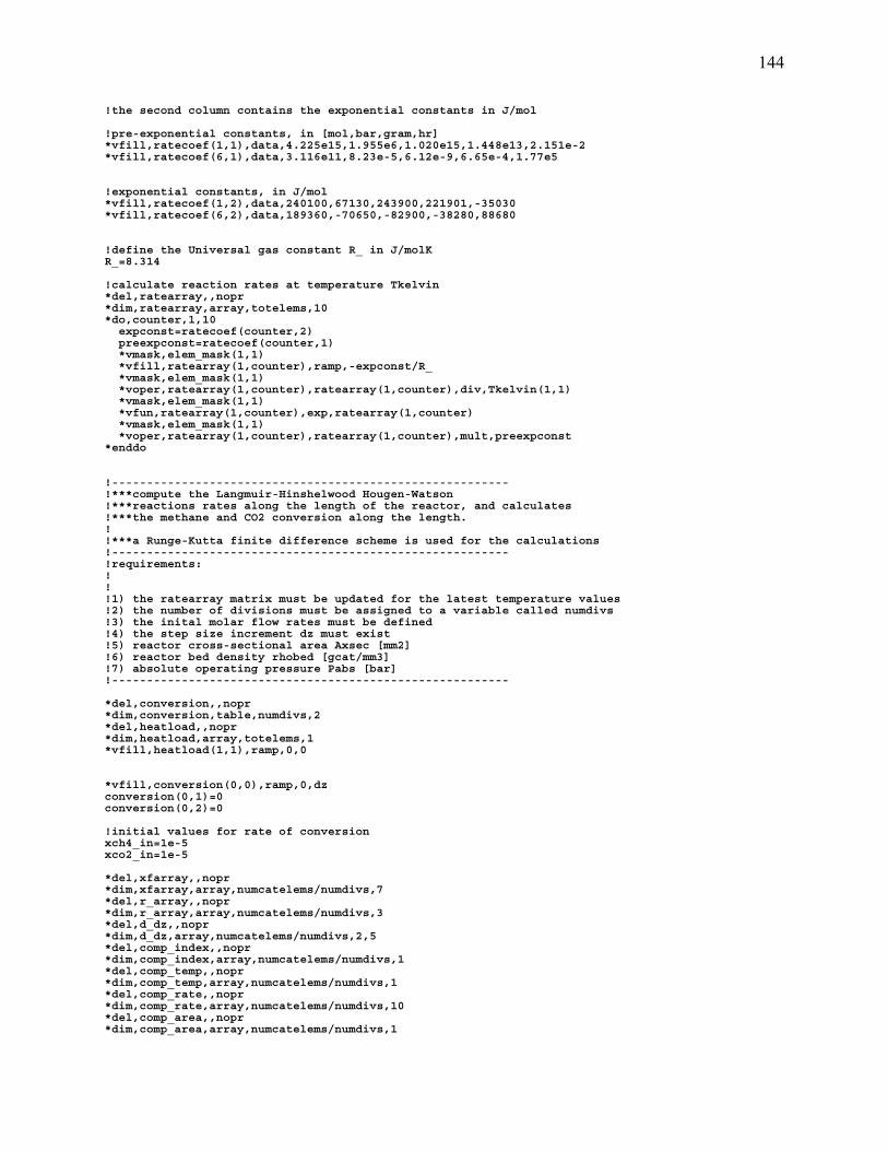
144
!the second column contains the exponential constants in J/mol !pre-exponential constants, in [mol,bar,gram,hr] *vfill,ratecoef(1,1),data,4.225e15,1.955e6,1.020e15,1.448e13,2.151e-2 *vfill,ratecoef(6,1),data,3.116e11,8.23e-5,6.12e-9,6.65e-4,1.77e5 !exponential constants, in J/mol *vfill,ratecoef(1,2),data,240100,67130,243900,221901,-35030 *vfill,ratecoef(6,2),data,189360,-70650,-82900,-38280,88680 !define the Universal gas constant R_ in J/molK R_=8.314 !calculate reaction rates at temperature Tkelvin *del,ratearray,,nopr *dim,ratearray,array,totelems,10 *do,counter,1,10 expconst=ratecoef(counter,2) preexpconst=ratecoef(counter,1) *vmask,elem_mask(1,1) *vfill,ratearray(1,counter),ramp,-expconst/R_ *vmask,elem_mask(1,1) *voper,ratearray(1,counter),ratearray(1,counter),div,Tkelvin(1,1) *vmask,elem_mask(1,1) *vfun,ratearray(1,counter),exp,ratearray(1,counter) *vmask,elem_mask(1,1) *voper,ratearray(1,counter),ratearray(1,counter),mult,preexpconst *enddo !--------------------------------------------------------- !***compute the Langmuir-Hinshelwood Hougen-Watson !***reactions rates along the length of the reactor, and calculates !***the methane and CO2 conversion along the length. ! !***a Runge-Kutta finite difference scheme is used for the calculations !--------------------------------------------------------- !requirements: ! ! !1) the ratearray matrix must be updated for the latest temperature values !2) the number of divisions must be assigned to a variable called numdivs !3) the inital molar flow rates must be defined !4) the step size increment dz must exist !5) reactor cross-sectional area Axsec [mm2] !6) reactor bed density rhobed [gcat/mm3] !7) absolute operating pressure Pabs [bar] !--------------------------------------------------------- *del,conversion,,nopr *dim,conversion,table,numdivs,2 *del,heatload,,nopr *dim,heatload,array,totelems,1 *vfill,heatload(1,1),ramp,0,0 *vfill,conversion(0,0),ramp,0,dz conversion(0,1)=0 conversion(0,2)=0 !initial values for rate of conversion xch4_in=1e-5 xco2_in=1e-5 *del,xfarray,,nopr *dim,xfarray,array,numcatelems/numdivs,7 *del,r_array,,nopr *dim,r_array,array,numcatelems/numdivs,3 *del,d_dz,,nopr *dim,d_dz,array,numcatelems/numdivs,2,5 *del,comp_index,,nopr *dim,comp_index,array,numcatelems/numdivs,1 *del,comp_temp,,nopr *dim,comp_temp,array,numcatelems/numdivs,1 *del,comp_rate,,nopr *dim,comp_rate,array,numcatelems/numdivs,10 *del,comp_area,,nopr *dim,comp_area,array,numcatelems/numdivs,1

145
*do,loop,1,2 *do,counter,loop,numdivs dz_=dz rateindex=counter *if,loop,eq,1,then dz_=dz/numdivs rateindex=1 *endif !compress full element range down to current division elements *voper,elem_mask(1,2),elem_mask(1,1),eq,rateindex *vmask,elem_mask(1,2) *vfill,elem_mask(1,2),ramp,1,1 *vmask,elem_mask(1,2) *vfun,comp_index(1,1),comp,elem_mask(1,2) *voper,comp_temp(1,1),Tkelvin(1,1),gath,comp_index(1,1) *voper,comp_area(1,1),elem_info(1,5),gath,comp_index(1,1) *do,comploop,1,10 *voper,comp_rate(1,comploop),ratearray(1,comploop),gath,comp_index(1,1) *enddo !partial pressures based on initial values *del,parpres,,nopr *dim,parpres,array,numcatelems/numdivs,8 !xch4 *vfill,parpres(1,1),ramp,xch4_in,0 !xco2 *vfill,parpres(1,2),ramp,xco2_in,0 *del,denomvector,,nopr *dim,denomvector,array,numcatelems/numdivs,1 *do,RKloop,1,4 !------------------------------------------ *voper,denomvector(1,1),parpres(1,1),mult,2*Fch4 *voper,denomvector(1,1),denomvector(1,1),add,Ftotal !ph2o *voper,parpres(1,3),parpres(1,1),add,parpres(1,2) *voper,parpres(1,3),parpres(1,3),mult,-Fch4 *voper,parpres(1,3),parpres(1,3),add,Fh2o *voper,parpres(1,3),parpres(1,3),mult,Pabs *voper,parpres(1,3),parpres(1,3),div,denomvector(1,1) !pch4 *voper,parpres(1,4),parpres(1,1),sub,1 *voper,parpres(1,4),parpres(1,4),mult,-Pabs*Fch4 *voper,parpres(1,4),parpres(1,4),div,denomvector(1,1) !pn2 *voper,parpres(1,5),Pabs*Fn2,div,denomvector(1,1) !pco2 *voper,parpres(1,6),parpres(1,2),mult,Fch4 *voper,parpres(1,6),parpres(1,6),add,Fco2 *voper,parpres(1,6),parpres(1,6),mult,Pabs *voper,parpres(1,6),parpres(1,6),div,denomvector(1,1) !ph2 *voper,parpres(1,7),parpres(1,1),mult,3 *voper,parpres(1,7),parpres(1,7),add,parpres(1,2) *voper,parpres(1,7),parpres(1,7),mult,Fch4 *voper,parpres(1,7),parpres(1,7),add,Fh2 *voper,parpres(1,7),parpres(1,7),mult,Pabs *voper,parpres(1,7),parpres(1,7),div,denomvector(1,1) !pco *voper,parpres(1,8),parpres(1,1),sub,parpres(1,2) *voper,parpres(1,8),parpres(1,8),mult,Fch4 *voper,parpres(1,8),parpres(1,8),add,Fco *voper,parpres(1,8),parpres(1,8),mult,Pabs *voper,parpres(1,8),parpres(1,8),div,denomvector(1,1) !Kco*pco *voper,xfarray(1,1),comp_rate(1,7),mult,parpres(1,8) !Kh2*ph2 *voper,xfarray(1,2),comp_rate(1,8),mult,parpres(1,7) !Kch4*pch4 *voper,xfarray(1,3),comp_rate(1,9),mult,parpres(1,4) !Kh2o*ph2o/ph2 *voper,xfarray(1,4),comp_rate(1,10),mult,parpres(1,3) *voper,xfarray(1,4),xfarray(1,4),div,parpres(1,7)

146
!(1+Kco*pco+Kh2*ph2+Kch4*pch4+Kh2o*ph2o/ph2)**2 *voper,xfarray(1,7),xfarray(1,1),add,1 *voper,xfarray(1,7),xfarray(1,7),add,xfarray(1,2) *voper,xfarray(1,7),xfarray(1,7),add,xfarray(1,3) *voper,xfarray(1,7),xfarray(1,7),add,xfarray(1,4) *vfun,xfarray(1,7),pwr,xfarray(1,7),2 !ph2**3*pco/K01 *vfun,xfarray(1,1),pwr,parpres(1,7),3 *voper,xfarray(1,1),xfarray(1,1),mult,parpres(1,8) *voper,xfarray(1,1),xfarray(1,1),div,comp_rate(1,4) !pch4*ph2o-ph2**3*pco/K01 *voper,xfarray(1,2),parpres(1,4),mult,parpres(1,3) *voper,xfarray(1,2),xfarray(1,2),sub,xfarray(1,1) !k1/ph2**2.5 *vfun,xfarray(1,1),pwr,parpres(1,7),2.5 *voper,xfarray(1,1),comp_rate(1,1),div,xfarray(1,1) !ph2*pco2/K02 *voper,xfarray(1,3),parpres(1,7),mult,parpres(1,6) *voper,xfarray(1,3),xfarray(1,3),div,comp_rate(1,5) !pco*ph2o-ph2*pco2/K02 *voper,xfarray(1,4),parpres(1,8),mult,parpres(1,3) *voper,xfarray(1,4),xfarray(1,4),sub,xfarray(1,3) !k2/ph2 *voper,xfarray(1,3),comp_rate(1,2),div,parpres(1,7) !ph2**4*pco2/K03 *vfun,xfarray(1,5),pwr,parpres(1,7),4 *voper,xfarray(1,5),xfarray(1,5),mult,parpres(1,6) *voper,xfarray(1,5),xfarray(1,5),div,comp_rate(1,6) !pch4*ph2o**2-ph2**4*pco2/K03 *vfun,xfarray(1,6),pwr,parpres(1,3),2 *voper,xfarray(1,6),xfarray(1,6),mult,parpres(1,4) *voper,xfarray(1,6),xfarray(1,6),sub,xfarray(1,5) !k3/ph2**3.5 *vfun,xfarray(1,5),pwr,parpres(1,7),3.5 *voper,xfarray(1,5),comp_rate(1,3),div,xfarray(1,5) !r1 CH4+H2O<->CO+3H2 *voper,r_array(1,1),xfarray(1,1),mult,xfarray(1,2) *voper,r_array(1,1),r_array(1,1),div,xfarray(1,7) !r2 CO+H2O<->CO2+H2 *voper,r_array(1,2),xfarray(1,3),mult,xfarray(1,4) *voper,r_array(1,2),r_array(1,2),div,xfarray(1,7) !r3 CH4+2H2O<->CO2+4H2 *voper,r_array(1,3),xfarray(1,5),mult,xfarray(1,6) *voper,r_array(1,3),r_array(1,3),div,xfarray(1,7) !slope of extents of conversion for ch4 and co2 *voper,d_dz(1,1,RKloop),r_array(1,1),add,r_array(1,3) *voper,d_dz(1,2,RKloop),r_array(1,2),add,r_array(1,3) *voper,d_dz(1,1,RKloop),d_dz(1,1,RKloop),mult,Axsec*rhobed*cat_factor/Fch4/3600 *voper,d_dz(1,2,RKloop),d_dz(1,2,RKloop),mult,Axsec*rhobed*cat_factor/Fch4/3600 !update partial pressures based on slope !xch4 *voper,parpres(1,1),d_dz(1,1,RKloop),mult,dz_/2 *voper,parpres(1,1),parpres(1,1),add,xch4_in !xco2 *voper,parpres(1,2),d_dz(1,2,RKloop),mult,dz_/2 *voper,parpres(1,2),parpres(1,2),add,xco2_in !------------------------------------------ *enddo !Runge-Kutta calculated rates, area-weighted *voper,d_dz(1,1,2),d_dz(1,1,2),mult,2 *voper,d_dz(1,2,2),d_dz(1,2,2),mult,2 *voper,d_dz(1,1,3),d_dz(1,1,3),mult,2 *voper,d_dz(1,2,3),d_dz(1,2,3),mult,2 *voper,d_dz(1,1,5),d_dz(1,1,1),add,d_dz(1,1,2)

147
*voper,d_dz(1,1,5),d_dz(1,1,5),add,d_dz(1,1,3) *voper,d_dz(1,1,5),d_dz(1,1,5),add,d_dz(1,1,4) *voper,d_dz(1,1,5),d_dz(1,1,5),div,6 *voper,d_dz(1,2,5),d_dz(1,2,1),add,d_dz(1,2,2) *voper,d_dz(1,2,5),d_dz(1,2,5),add,d_dz(1,2,3) *voper,d_dz(1,2,5),d_dz(1,2,5),add,d_dz(1,2,4) *voper,d_dz(1,2,5),d_dz(1,2,5),div,6 totarea=areavector(rateindex,1) !--------------------------------------------------------- !***calculate the change in molar flow rates of the species !***for each catalyst element along the reactor length, based on the calculated !***extents of conversion. The change in molar flow rates and temperature is !***then used to calculate the reaction heat duty. !--------------------------------------------------------- *del,molflowin,,nopr *dim,molflowin,array,numcatelems/numdivs,7 *del,molflowout,,nopr *dim,molflowout,array,numcatelems/numdivs,7 !columns contain molar flow rates [mol/s] in the following order: !CH4 H2O CO2 CO H2 N2 total !molar flow rates are not normalized to the element areas - full flow rate !is considered for each element, and normalization is done on the enthalpy !molar flow rate in !column 1 - CH4 *vfill,molflowin(1,1),ramp,(1-xch4_in)*Fch4,0 !column 2 - H2O *vfill,molflowin(1,2),ramp,Fh2o-(xch4_in+xco2_in)*Fch4,0 !column 3 - CO2 *vfill,molflowin(1,3),ramp,Fco2+xco2_in*Fch4,0 !column 4 - CO *vfill,molflowin(1,4),ramp,Fco+Fch4*(xch4_in-xco2_in),0 !column 5 - H2 *vfill,molflowin(1,5),ramp,Fh2+Fch4*(3*xch4_in+xco2_in),0 !column 6 - N2 *vfill,molflowin(1,6),ramp,Fn2,0 !column 7 - total *voper,molflowin(1,7),molflowin(1,1),add,molflowin(1,2) *voper,molflowin(1,7),molflowin(1,7),add,molflowin(1,3) *voper,molflowin(1,7),molflowin(1,7),add,molflowin(1,4) *voper,molflowin(1,7),molflowin(1,7),add,molflowin(1,5) *voper,molflowin(1,7),molflowin(1,7),add,molflowin(1,6) !---------------------------------------------------- !molar flow rate out !temporarily place x_in+dx/dz*dz into columns 6 (ch4) and7 (co2) *voper,molflowout(1,6),d_dz(1,1,5),mult,dz_ *voper,molflowout(1,6),molflowout(1,6),add,xch4_in *voper,molflowout(1,7),d_dz(1,2,5),mult,dz_ *voper,molflowout(1,7),molflowout(1,7),add,xco2_in !column 1 - CH4 *voper,molflowout(1,1),molflowout(1,6),sub,1 *voper,molflowout(1,1),molflowout(1,1),mult,-Fch4 !column 2 - H2O *voper,molflowout(1,2),molflowout(1,6),add,molflowout(1,7) *voper,molflowout(1,2),molflowout(1,2),mult,-Fch4 *voper,molflowout(1,2),molflowout(1,2),add,Fh2o !column 3 - CO2 *voper,molflowout(1,3),molflowout(1,7),mult,Fch4 *voper,molflowout(1,3),molflowout(1,3),add,Fco2 !column 4 - CO *voper,molflowout(1,4),molflowout(1,6),sub,molflowout(1,7) *voper,molflowout(1,4),molflowout(1,4),mult,Fch4 *voper,molflowout(1,4),molflowout(1,4),add,Fco

148
!column 5 - H2 *voper,molflowout(1,5),molflowout(1,6),mult,3 *voper,molflowout(1,5),molflowout(1,5),add,molflowout(1,7) *voper,molflowout(1,5),molflowout(1,5),mult,Fch4 *voper,molflowout(1,5),molflowout(1,5),add,Fh2 !column 6 - N2 *vfill,molflowout(1,6),ramp,Fn2,0 !column 7 - total *voper,molflowout(1,7),molflowout(1,1),add,molflowout(1,2) *voper,molflowout(1,7),molflowout(1,7),add,molflowout(1,3) *voper,molflowout(1,7),molflowout(1,7),add,molflowout(1,4) *voper,molflowout(1,7),molflowout(1,7),add,molflowout(1,5) *voper,molflowout(1,7),molflowout(1,7),add,molflowout(1,6) !---------------------------------------------------- *del,enthin,,nopr *del,enthout,,nopr *dim,enthin,array,numcatelems/numdivs,6 *dim,enthout,array,numcatelems/numdivs,6 !enthalpy of each of the reacting species is calculated using straight-line !regression data from ppds software (data over 673K - 1073K range). !enthalpy in [mW] is calculated by the species molar flow rate in and out !of each segment, and the total isothermal enthalpy change for each element !at the element surface temperature is calculated. !column 1 - CH4 *voper,enthin(1,1),comp_temp(1,1),mult,67.792 *voper,enthin(1,1),enthin(1,1),add,-29151 *voper,enthin(1,1),enthin(1,1),add,-74400 *voper,enthin(1,1),enthin(1,1),mult,molflowin(1,1) *voper,enthout(1,1),comp_temp(1,1),mult,67.792 *voper,enthout(1,1),enthout(1,1),add,-29151 *voper,enthout(1,1),enthout(1,1),add,-74400 *voper,enthout(1,1),enthout(1,1),mult,molflowout(1,1) !column 2 - H2O *voper,enthin(1,2),comp_temp(1,1),mult,39.847 *voper,enthin(1,2),enthin(1,2),add,-13834 *voper,enthin(1,2),enthin(1,2),add,-241830 *voper,enthin(1,2),enthin(1,2),mult,molflowin(1,2) *voper,enthout(1,2),comp_temp(1,1),mult,39.847 *voper,enthout(1,2),enthout(1,2),add,-13834 *voper,enthout(1,2),enthout(1,2),add,-241830 *voper,enthout(1,2),enthout(1,2),mult,molflowout(1,2) !column 3 - CO2 *voper,enthin(1,3),comp_temp(1,1),mult,52.691 *voper,enthin(1,3),enthin(1,3),add,-19316 *voper,enthin(1,3),enthin(1,3),add,-393520 *voper,enthin(1,3),enthin(1,3),mult,molflowin(1,3) *voper,enthout(1,3),comp_temp(1,1),mult,52.691 *voper,enthout(1,3),enthout(1,3),add,-19316 *voper,enthout(1,3),enthout(1,3),add,-393520 *voper,enthout(1,3),enthout(1,3),mult,molflowout(1,3) !column 4 - CO *voper,enthin(1,4),comp_temp(1,1),mult,32.345 *voper,enthin(1,4),enthin(1,4),add,-10670 *voper,enthin(1,4),enthin(1,4),add,-110530 *voper,enthin(1,4),enthin(1,4),mult,molflowin(1,4) *voper,enthout(1,4),comp_temp(1,1),mult,32.345 *voper,enthout(1,4),enthout(1,4),add,-10670 *voper,enthout(1,4),enthout(1,4),add,-110530 *voper,enthout(1,4),enthout(1,4),mult,molflowout(1,4) !column 5 - H2 *voper,enthin(1,5),comp_temp(1,1),mult,29.977 *voper,enthin(1,5),enthin(1,5),add,-9292 *voper,enthin(1,5),enthin(1,5),mult,molflowin(1,5) *voper,enthout(1,5),comp_temp(1,1),mult,29.977 *voper,enthout(1,5),enthout(1,5),add,-9292 *voper,enthout(1,5),enthout(1,5),mult,molflowout(1,5) !column 6 - total *voper,enthin(1,6),enthin(1,1),add,enthin(1,2) *voper,enthin(1,6),enthin(1,6),add,enthin(1,3) *voper,enthin(1,6),enthin(1,6),add,enthin(1,4)

149
*voper,enthin(1,6),enthin(1,6),add,enthin(1,5) *voper,enthin(1,6),enthin(1,6),mult,1000 *voper,enthout(1,6),enthout(1,1),add,enthout(1,2) *voper,enthout(1,6),enthout(1,6),add,enthout(1,3) *voper,enthout(1,6),enthout(1,6),add,enthout(1,4) *voper,enthout(1,6),enthout(1,6),add,enthout(1,5) *voper,enthout(1,6),enthout(1,6),mult,1000 !area-weight the enthalpies in and out *voper,enthin(1,6),enthin(1,6),mult,comp_area(1,1) *voper,enthin(1,6),enthin(1,6),div,totarea *voper,enthout(1,6),enthout(1,6),mult,comp_area(1,1) *voper,enthout(1,6),enthout(1,6),div,totarea !------------------------------------------ !add the enthalpy change to the heat load vector *del,temp1,,nopr *dim,temp1,array,totelems,1 *vfun,temp1(1,1),not,elem_mask(1,2) *voper,heatload(1,1),heatload(1,1),mult,temp1(1,1) *vfill,temp1(1,1),ramp,0 *voper,temp1(1,1),enthin(1,6),scat,comp_index(1,1) *voper,heatload(1,1),heatload(1,1),add,temp1(1,1) *vfill,temp1(1,1),ramp,0 *voper,temp1(1,1),enthout(1,6),scat,comp_index(1,1) *voper,heatload(1,1),heatload(1,1),sub,temp1(1,1) *voper,d_dz(1,1,5),d_dz(1,1,5),mult,comp_area(1,1) *voper,d_dz(1,2,5),d_dz(1,2,5),mult,comp_area(1,1) *voper,d_dz(1,1,5),d_dz(1,1,5),div,totarea *voper,d_dz(1,2,5),d_dz(1,2,5),div,totarea *vscfun,mch4,sum,d_dz(1,1,5) *vscfun,mco2,sum,d_dz(1,2,5) !calculate conversion extent xch4=xch4_in+mch4*dz_ xco2=xco2_in+mco2*dz_ conversion(counter,1)=xch4 conversion(counter,2)=xco2 xch4_in=xch4 xco2_in=xco2 *enddo *if,loop,eq,1,then conversion(1,1)=xch4 conversion(1,2)=xco2 *endif *enddo !--------------------------------------------------------- !***calculate the bulk molar flow rates of species along !***the reactor length, based on the calculated extent of conversion. !--------------------------------------------------------- *del,molflow,,nopr *dim,molflow,table,numdivs,7 *vfun,molflow(0,0),copy,conversion(0,0) !columns contain molar flow rates [mol/s] in the following order: !CH4 H2O CO2 CO H2 N2 total !column 1 - CH4 *voper,molflow(0,1),1,sub,conversion(0,1) *voper,molflow(0,1),molflow(0,1),mult,Fch4 !column 2 - H2O *voper,molflow(0,2),conversion(0,1),add,conversion(0,2) *voper,molflow(0,2),molflow(0,2),mult,-Fch4 *voper,molflow(0,2),molflow(0,2),add,Fh2o !column 3 - CO2 *voper,molflow(0,3),conversion(0,2),mult,Fch4

150
*voper,molflow(0,3),molflow(0,3),add,Fco2 !column 4 - CO *voper,molflow(0,4),conversion(0,1),sub,conversion(0,2) *voper,molflow(0,4),molflow(0,4),mult,Fch4 *voper,molflow(0,4),molflow(0,4),add,Fco !column 5 - H2 *voper,molflow(0,5),conversion(0,1),mult,3 *voper,molflow(0,5),molflow(0,5),add,conversion(0,2) *voper,molflow(0,5),molflow(0,5),mult,Fch4 *voper,molflow(0,5),molflow(0,5),add,Fh2 !column 6 - N2 *vfill,molflow(0,6),ramp,Fn2 !column 7 - total *voper,molflow(0,7),molflow(0,1),add,molflow(0,2) *voper,molflow(0,7),molflow(0,7),add,molflow(0,3) *voper,molflow(0,7),molflow(0,7),add,molflow(0,4) *voper,molflow(0,7),molflow(0,7),add,molflow(0,5) *voper,molflow(0,7),molflow(0,7),add,molflow(0,6) !---------------------------------------------------- !***apply the chemical reaction load to the catalyst !***surface effect elements !--------------------------------------------------------- /solu *del,hgenvector,,nopr *dim,hgenvector,array,numcatelems,2 *vmask,elem_mask(1,1) *voper,heatload(1,1),heatload(1,1),div,elem_info(1,5) *get,t_catalyst,rcon,cat_real,7 *vmask,elem_mask(1,1) *voper,heatload(1,1),heatload(1,1),div,t_catalyst *voper,heatload(1,1),heatload(1,1),mult,sector *vmask,elem_mask(1,1) *vfun,hgenvector(1,1),comp,elem_mask(1,3) *vmask,elem_mask(1,1) *vfun,hgenvector(1,2),comp,heatload(1,1) allsel *do,counter,1,numcatelems bfe,hgenvector(counter,1),hgen,,hgenvector(counter,2) *enddo /solu allsel solve /post1 !***calculate the catalyst surface temperature !***at each catalyst surface element of the reactor !--------------------------------------------------------- !requirements: ! ! !1) solution !2) elem_info matrix !3) maskvector !5) reacting flow real constant # assigned to variable name reacflow !--------------------------------------------------------- /post1 allsel *get,totnodes,node,,num,maxd *del,nodetemps,,nopr !================================================================= !NOTE - ANSYS VERSION 11 HAS A BUG IN THE *VOPER,,,GATH COMMAND !TO MAKE THIS FILE WORK CORRECTLY IN VERSION 11, THE NUMBER OF !ROWS IN THE ARRAY nodetemps MUST BE GREATER THAN OR EQUAL !TO totelems

151
!================================================================= arraysize=max(totnodes,totelems) *dim,nodetemps,array,arraysize,1 *vget,nodetemps(1,1),node,1,temp *del,elemtemparray,,nopr *dim,elemtemparray,array,totelems,5 !columns 1-4 are the nodal temperatures for the element *vmask,elem_mask(1,1) *voper,elemtemparray(1,1),nodetemps(1,1),gath,elem_info(1,1) *vmask,elem_mask(1,1) *voper,elemtemparray(1,2),nodetemps(1,1),gath,elem_info(1,2) *vmask,elem_mask(1,1) *voper,elemtemparray(1,3),nodetemps(1,1),gath,elem_info(1,3) *vmask,elem_mask(1,1) *voper,elemtemparray(1,4),nodetemps(1,1),gath,elem_info(1,4) !column 5 is the element average temperature, from the 4 nodal temps *vmask,elem_mask(1,1) *voper,elemtemparray(1,5),elemtemparray(1,1),add,elemtemparray(1,2) *vmask,elem_mask(1,1) *voper,elemtemparray(1,5),elemtemparray(1,5),add,elemtemparray(1,3) *vmask,elem_mask(1,1) *voper,elemtemparray(1,5),elemtemparray(1,5),add,elemtemparray(1,4) *vmask,elem_mask(1,1) *voper,elemtemparray(1,5),elemtemparray(1,5),div,4 !***update the temperature (in Kelvin) used to calculate !***the surface reaction rate !--------------------------------------------------------- !requirements: ! ! !1) elemtemparray vector !2) Tkelvin vector !--------------------------------------------------------- relaxdefault=2 maxch_allow=20 *del,changecheck,,nopr *dim,changecheck,array,numcatelems,4 *vmask,elem_mask(1,1) *vfun,changecheck(1,1),comp,Tkelvin(1,1) *vmask,elem_mask(1,1) *vfun,changecheck(1,2),comp,elemtemparray(1,5) *voper,changecheck(1,2),changecheck(1,2),add,273.15 *vabs,1 *voper,changecheck(1,3),changecheck(1,2),sub,changecheck(1,1) *vscfun,maxchange,max,changecheck(1,3) criterion=1 relax=relaxdefault *dowhile,criterion *voper,changecheck(1,3),changecheck(1,1),mult,relax *voper,changecheck(1,3),changecheck(1,3),add,changecheck(1,2) *voper,changecheck(1,3),changecheck(1,3),div,relax+1 *vabs,1 *voper,changecheck(1,4),changecheck(1,1),sub,changecheck(1,3) *vscfun,maxcheck,max,changecheck(1,4) criterion=maxcheck-maxch_allow relax=relax+1 *enddo *vmask,elem_mask(1,1) *vfun,Tkelvin(1,1),expa,changecheck(1,3) terminate=maxchange-term_crit !***calculate the fluid properties of the reacting flow !***each fluid element has a seprate material property id, and the properties

152
!***are calculated based on flow composition and temperature from the previous !***solution. !--------------------------------------------------------- !requirements: ! ! !1) solution !2) elem_info matrix !3) molflow array !4) reacting flow real constant # assigned to variable name reacflow !5) operating pressure, Pabs !--------------------------------------------------------- /post1 allsel !--------------------------------------------------- !***fill a vector, nodetemps, with all of the nodal temperatures *get,totnodes,node,,num,maxd *del,nodetemps,,nopr *dim,nodetemps,array,totnodes,1 *vget,nodetemps(1,1),node,1,temp *voper,nodetemps(1,1),nodetemps(1,1),max,20 !--------------------------------------------------- !--------------------------------------------------- !***create an element array with temperatures for nodes 1 and 2, !***the average of those two temps, the z-direction centroid, and !***a masking vector that selects only the reacting flow Fluid116s *get,totelems,elem,,num,maxd *del,elemtemparray,,nopr *dim,elemtemparray,array,totelems,6 !column 1 is the element number *vfill,elemtemparray(1,1),ramp,1,1 !columns 2-3 are the nodal temperatures for the element *voper,elemtemparray(1,2),nodetemps(1,1),gath,elem_info(1,1) *voper,elemtemparray(1,3),nodetemps(1,1),gath,elem_info(1,2) !column 4 is the mean element temperature *voper,elemtemparray(1,4),elemtemparray(1,2),add,elemtemparray(1,3) *voper,elemtemparray(1,4),elemtemparray(1,4),div,2 !column 5 is element centroid location in the z direction *vget,elemtemparray(1,5),elem,1,cent,z !column 6 is a masking vector for the reacting flow elements esels,s,real,,reacflow *vget,elemtemparray(1,6),elem,1,esel !--------------------------------------------------- !--------------------------------------------------- !***create an array with each row corresponding to the beginning/end !***of a row of elements in the reacting region. !***this array contains the reacting flow element number, material id, !***mean element temperature, and flow molar fractions at that location *del,flowstatarray,,nopr *dim,flowstatarray,array,numdivs+1,9 *del,junk,,nopr *dim,junk,array,numdivs+2,1 *vmask,elemtemparray(1,6) *vfun,flowstatarray(1,1),comp,elemtemparray(1,1) *vmask,elemtemparray(1,6) *vfun,flowstatarray(1,2),comp,elemtemparray(1,5) *voper,flowstatarray(1,2),flowstatarray(1,2),mult,1000 *vmask,elemtemparray(1,6) *vfun,flowstatarray(1,3),comp,elemtemparray(1,4) *voper,flowstatarray(1,3),flowstatarray(1,3),add,273.15 *moper,junk(1,1),flowstatarray(1,1),sort,flowstatarray(1,2) *vfill,flowstatarray(1,2),ramp,101,1 *del,junk,,nopr /prep7 emodif,flowstatarray(1:numdivs+1,1),mat,flowstatarray(1:numdivs+1,2) !columns 4-9 are molar fractions of CH4 H2O CO2 CO H2 N2 *voper,flowstatarray(1,4),molflow(0,1),div,molflow(0,7) *voper,flowstatarray(1,5),molflow(0,2),div,molflow(0,7) *voper,flowstatarray(1,6),molflow(0,3),div,molflow(0,7) *voper,flowstatarray(1,7),molflow(0,4),div,molflow(0,7) *voper,flowstatarray(1,8),molflow(0,5),div,molflow(0,7) *voper,flowstatarray(1,9),molflow(0,6),div,molflow(0,7) !---------------------------------------------------

153
!====================================================================== !calculate properties of pure components, and mixture properties !coefficient matrix !CH4 H2O CO2 CO H2 N2 *del,propcoef,,nopr *dim,propcoef,array,14,6 *vfill,propcoef(1,1),data,3.3295e4,8.0295e4,2.1018e3 *vfill,propcoef(4,1),data,4.213e4,9.951e2,1.323e-5 *vfill,propcoef(7,1),data,1.798e-1,7.18e2,-8.9e3 *vfill,propcoef(10,1),data,1.266e-3,8.031e-1,9.6e2 *vfill,propcoef(13,1),data,-6.12e4,16.04303 *vfill,propcoef(1,2),data,3.3359E+04,2.6798E+04,2.6093E+03 *vfill,propcoef(4,2),data,8.8880E+03,1.1676E+03,2.6986E-06 *vfill,propcoef(7,2),data,4.9800E-01,1.2577E+03,-1.9570E+04 *vfill,propcoef(10,2),data,6.9770E-05,1.1243E+00,8.4490E+02 *vfill,propcoef(13,2),data,-1.4885E+05,18.01534 *vfill,propcoef(1,3),data,2.9370E+04,3.4540E+04,-1.4280E+03 *vfill,propcoef(4,3),data,2.6400E+04,5.8800E+02,2.1480E-06 *vfill,propcoef(7,3),data,4.6000E-01,2.9000E+02,0.0000E+00 *vfill,propcoef(10,3),data,3.6900E+00,-3.8380E-01,9.6400E+02 *vfill,propcoef(13,3),data,1.8600E+06,44.00995 *vfill,propcoef(1,4),data,2.9108E+04,8.7730E+03,3.0851E+03 *vfill,propcoef(4,4),data,8.4553E+03,1.5382E+03,1.1127E-06 *vfill,propcoef(7,4),data,5.3380E-01,9.4700E+01,0.0000E+00 *vfill,propcoef(10,4),data,8.3900E-04,6.4090E-01,8.6050E+01 *vfill,propcoef(13,4),data,0.0000E+00,28.01055 *vfill,propcoef(1,5),data,2.7617E+04,9.5600E+03,2.4660E+03 *vfill,propcoef(4,5),data,3.7600E+03,5.6760E+02,1.5600E-07 *vfill,propcoef(7,5),data,7.0600E-01,-5.8700E+00,2.1000E+02 *vfill,propcoef(10,5),data,2.5470E-03,7.4440E-01,9.0000E+00 *vfill,propcoef(13,5),data,0.0000E+00,2.01594 *vfill,propcoef(1,6),data,2.9105E+04,8.6149E+03,1.7016E+03 *vfill,propcoef(4,6),data,1.0347E+02,9.0979E+02,7.6320E-07 *vfill,propcoef(7,6),data,5.8823E-01,6.7750E+01,0.0000E+00 *vfill,propcoef(10,6),data,3.5100E-04,7.6520E-01,2.5767E+01 *vfill,propcoef(13,6),data,0.0000E+00,28.0134 !------------------------------------------------ *del,properties,,nopr *del,temparray,,nopr *del,tvector,,nopr *del,molwtarray,,nopr *del,specvisc,,,nopr *del,speccond,,,nopr *del,Aij,,nopr *dim,properties,array,numdivs+1,4 *dim,temparray,array,numdivs+1,3 *dim,tvector,array,numdivs+1,1 *dim,molwtarray,array,numdivs+1,7 *dim,specvisc,array,numdivs+1,6 *dim,speccond,array,numdivs+1,6 *dim,Aij,array,numdivs+1,6,6 *vfun,tvector(1,1),copy,flowstatarray(1,3) *vfill,molwtarray(1,7),ramp,0,0 *do,counter,1,6 molwt=propcoef(14,counter) *voper,molwtarray(1,counter),flowstatarray(1,counter+3),mult,molwt *voper,molwtarray(1,7),molwtarray(1,7),add,molwtarray(1,counter) *enddo !Specific Heat [J/kgK] *vfill,properties(1,1),ramp,0,0 *do,counter,1,6 Acoef=propcoef(1,counter) Bcoef=propcoef(2,counter)

154
Ccoef=propcoef(3,counter) Dcoef=propcoef(4,counter) Ecoef=propcoef(5,counter) *voper,temparray(1,1),Ccoef,div,tvector(1,1) *vfun,temparray(1,2),sinh,temparray(1,1) *voper,temparray(1,1),temparray(1,1),div,temparray(1,2) *vfun,temparray(1,1),pwr,temparray(1,1),2 *voper,temparray(1,1),temparray(1,1),mult,Bcoef *voper,temparray(1,2),Ecoef,div,tvector(1,1) *vfun,temparray(1,3),cosh,temparray(1,2) *voper,temparray(1,2),temparray(1,2),div,temparray(1,3) *vfun,temparray(1,2),pwr,temparray(1,2),2 *voper,temparray(1,2),temparray(1,2),mult,Dcoef *voper,temparray(1,1),temparray(1,1),add,temparray(1,2) *voper,temparray(1,1),temparray(1,1),add,Acoef *voper,temparray(1,1),temparray(1,1),mult,flowstatarray(1,counter+3) *voper,properties(1,1),properties(1,1),add,temparray(1,1) *enddo *voper,properties(1,1),properties(1,1),div,molwtarray(1,7) !--------------------------------------------------------- !Viscosity [Ns/m2] (used in mixture conductivity calculation) *do,counter,1,6 Acoef=propcoef(6,counter) Bcoef=propcoef(7,counter) Ccoef=propcoef(8,counter) Dcoef=propcoef(9,counter) molwt=propcoef(14,counter) *voper,temparray(1,1),Ccoef,div,tvector(1,1) *voper,temparray(1,2),Dcoef,div,tvector(1,1) *voper,temparray(1,2),temparray(1,2),div,tvector(1,1) *voper,temparray(1,1),temparray(1,1),add,temparray(1,2) *voper,temparray(1,1),temparray(1,1),add,1 *voper,temparray(1,1),Acoef,div,temparray(1,1) *vfun,temparray(1,2),pwr,tvector(1,1),Bcoef *voper,temparray(1,1),temparray(1,1),mult,temparray(1,2) *vfun,specvisc(1,counter),copy,temparray(1,1) *enddo !--------------------------------------------------------- !Thermal Conductivity [W/mK] !calculated using the Mason and Saxena formulation of the Wassiljewa Equation *vfill,properties(1,3),ramp,0,0 *vfill,properties(1,4),ramp,0,0 *do,counter,1,6 Acoef=propcoef(10,counter) Bcoef=propcoef(11,counter) Ccoef=propcoef(12,counter) Dcoef=propcoef(13,counter) molwt=propcoef(14,counter) *voper,temparray(1,1),Ccoef,div,tvector(1,1) *voper,temparray(1,2),Dcoef,div,tvector(1,1) *voper,temparray(1,2),temparray(1,2),div,tvector(1,1) *voper,temparray(1,1),temparray(1,1),add,temparray(1,2) *voper,temparray(1,1),temparray(1,1),add,1 *voper,temparray(1,1),Acoef,div,temparray(1,1) *vfun,temparray(1,2),pwr,tvector(1,1),Bcoef *voper,temparray(1,1),temparray(1,1),mult,temparray(1,2) *vfun,speccond(1,counter),copy,temparray(1,1) *enddo *do,counteri,1,6 *do,counterj,1,6 molwti=propcoef(14,counteri) molwtj=propcoef(14,counterj) *voper,temparray(1,1),specvisc(1,counteri),div,specvisc(1,counterj) *vfun,temparray(1,1),pwr,temparray(1,1),0.5 *voper,temparray(1,1),temparray(1,1),mult,(molwtj/molwti)**0.25 *voper,temparray(1,1),temparray(1,1),add,1 *vfun,temparray(1,1),pwr,temparray(1,1),2 *voper,Aij(1,counteri,counterj),temparray(1,1),mult,1.065/(8*(1+molwti/molwtj))**0.5

155
*enddo *enddo *do,counter,1,6 *vfill,Aij(1,counter,counter),ramp,0,0 *enddo *do,counteri,1,6 *vfill,temparray(1,1),ramp,0,0 *do,counterj,1,6 *voper,temparray(1,2),flowstatarray(1,counterj+3),div,flowstatarray(1,counteri+3) *vcum,1 *voper,temparray(1,1),temparray(1,2),mult,Aij(1,counteri,counterj) *enddo *voper,temparray(1,1),temparray(1,1),add,1 *vcum,1 *voper,properties(1,3),speccond(1,counteri),div,temparray(1,1) *enddo !--------------------------------------------------------- !Density [gm/mm3] *voper,properties(1,4),molwtarray(1,7),div,tvector(1,1) *voper,properties(1,4),properties(1,4),mult,Pabs *voper,properties(1,4),properties(1,4),div,8.314 *voper,properties(1,4),properties(1,4),mult,1e-4 !====================================================================== !--------------------------------------------------------- !***update fluid material properties /prep7 mp,c,flowstatarray(1:numdivs+1,2),properties(1:numdivs+1,1) mp,kxx,flowstatarray(1:numdivs+1,2),properties(1:numdivs+1,3) mp,dens,flowstatarray(1:numdivs+1,2),properties(1:numdivs+1,4) !--------------------------------------------------------- !***calculate the film coefficient of the reacting flow !***moving through the reactor, and fills a table with the film coefficients !***vs. z location !--------------------------------------------------------- !requirements: ! ! !1) mesh !2) properties matrix !3) Nusselt number, Nu_reacflow !4) hydraulic diameter, Dh_reacflow, in [mm] !5) reacting flow real constant # assigned to variable name reacflow !--------------------------------------------------------- !--------------------------------------------------- !***fill a vector, nodetemps, with all of the nodal z locations !***and a masking vector *get,totnodes,node,,num,maxd *del,nodez,,nopr *dim,nodez,array,totnodes,2 *vget,nodez(1,1),node,1,loc,z esel,s,real,,reacflow nsle esel,s,ename,,152 nsle,r *vget,nodez(1,2),node,1,nsel !--------------------------------------------------- !--------------------------------------------------- !***compress and sort the z location vector into a new vector *del,nodez2,,nopr *dim,nodez2,array,numdivs,1 *vmask,nodez(1,2) *vfun,nodez2(1,1),comp,nodez(1,1) *moper,nodez(1,2),nodez2(1,1),sort,nodez2(1,1) !--------------------------------------------------- !--------------------------------------------------- !***create a film coefficient table [mW/mm2K] *del,filmcoef,,nopr *dim,filmcoef,table,numdivs,1,1,z

156
*voper,filmcoef(1,1),properties(1,3),mult,Nu_reacflow/Dh_reacflow *vfun,filmcoef(1,0),copy,nodez2(1,1) !--------------------------------------------------- !--------------------------------------------------- !***apply convection loading /solu esel,s,real,,reacflow nsle esln esel,r,ename,,152 sfe,all,,conv,,%filmcoef% allsel !--------------------------------------------------- allsel *enddo


![Visual Interaction with Dimensionality Reduction: A ... · PDF fileimprove performance by mitigating the curse of dimensionality [15]. Faced with a ... overcome this challenge is to](https://static.fdocuments.in/doc/165x107/5a9de0ee7f8b9aee528d99d9/visual-interaction-with-dimensionality-reduction-a-performance-by-mitigating.jpg)