A mixed and discontinuous Galerkin finite volume element method for incompressible miscible...
28
A Mixed and Discontinuous Galerkin Finite Volume Element Method for Incompressible Miscible Displacement Problems in Porous Media Sarvesh Kumar Department of Mathematics, Birla Institute of Technology and Science, Pilani-K.K. Birla Goa Campus, Zuarinagar-403726, Goa, India Received 20 July 2010; accepted 1 April 2011 Published online 13 May 2011 in Wiley Online Library (wileyonlinelibrary.com). DOI 10.1002/num.20684 The incompressible miscible displacement problem in porous media is modeled by a coupled system of two nonlinear partial differential equations, the pressure-velocity equation and the concentration equation. In this article, we present a mixed finite volume element method for the approximation of pressure-velocity equation and a discontinuous Galerkin finite volume element method for the concentration equation. A pri- ori error estimates in L ∞ (L 2 ) are derived for velocity, pressure, and concentration. Numerical results are presented to substantiate the validity of the theoretical results. © 2011 Wiley Periodicals, Inc. Numer Methods Partial Differential Eq 28: 1354–1381, 2012 Keywords: discontinuous Galerkin methods; error estimates; finite volume element methods; miscible displacement problems; mixed methods; numerical experiments I. INTRODUCTION A mathematical model describing miscible displacement of one incompressible fluid by another in a horizontal porous medium reservoir ⊂ R 2 with boundary ∂ of unit thickness over a time period of J = (0, T ] is given by u =− κ(x) µ(c) ∇p ∀(x , t) ∈ × J , (1.1) ∇· u = q ∀(x , t) ∈ × J , (1.2) φ(x) ∂c ∂t −∇· (D(u)∇c − uc) = g(x , t , c) = ( ˜ c − c)q ∀(x , t) ∈ × J , (1.3) Correspondence to: Sarvesh Kumar, Department of Mathematics, Birla Institute of Technology and Science, Pilani-K.K. Birla Goa Campus, Zuarinagar-403726, Goa, India (e-mail: [email protected]) © 2011 Wiley Periodicals, Inc.
-
Upload
sarvesh-kumar -
Category
Documents
-
view
213 -
download
0
Transcript of A mixed and discontinuous Galerkin finite volume element method for incompressible miscible...

A Mixed and Discontinuous Galerkin FiniteVolume Element Method for IncompressibleMiscible Displacement Problems in Porous MediaSarvesh KumarDepartment of Mathematics, Birla Institute of Technology and Science, Pilani-K.K. BirlaGoa Campus, Zuarinagar-403726, Goa, India
Received 20 July 2010; accepted 1 April 2011Published online 13 May 2011 in Wiley Online Library (wileyonlinelibrary.com).DOI 10.1002/num.20684
The incompressible miscible displacement problem in porous media is modeled by a coupled system of twononlinear partial differential equations, the pressure-velocity equation and the concentration equation. Inthis article, we present a mixed finite volume element method for the approximation of pressure-velocityequation and a discontinuous Galerkin finite volume element method for the concentration equation. A pri-ori error estimates in L∞(L2) are derived for velocity, pressure, and concentration. Numerical results arepresented to substantiate the validity of the theoretical results. © 2011 Wiley Periodicals, Inc. Numer MethodsPartial Differential Eq 28: 1354–1381, 2012
Keywords: discontinuous Galerkin methods; error estimates; finite volume element methods; miscibledisplacement problems; mixed methods; numerical experiments
I. INTRODUCTION
A mathematical model describing miscible displacement of one incompressible fluid by anotherin a horizontal porous medium reservoir � ⊂ R
2 with boundary ∂� of unit thickness over a timeperiod of J = (0, T ] is given by
u = −κ(x)
µ(c)∇p ∀(x, t) ∈ � × J , (1.1)
∇ · u = q ∀(x, t) ∈ � × J , (1.2)
φ(x)∂c
∂t− ∇ · (D(u)∇c − uc) = g(x, t , c) = (c − c)q ∀(x, t) ∈ � × J , (1.3)
Correspondence to: Sarvesh Kumar, Department of Mathematics, Birla Institute of Technology and Science, Pilani-K.K.Birla Goa Campus, Zuarinagar-403726, Goa, India (e-mail: [email protected])
© 2011 Wiley Periodicals, Inc.
GALERKIN FINITE VOLUME ELEMENT METHOD 1355
with boundary conditions
u · n = 0 ∀(x, t) ∈ ∂� × J , (1.4)
(D(u)∇c − uc) · n = 0 ∀(x, t) ∈ ∂� × J , (1.5)
and initial condition
c(x, 0) = c0(x) ∀x ∈ �, (1.6)
where x = (x1, x2) ∈ �, u(x, t) = (u1(x, t), u2(x, t)), and p(x, t) are, respectively, the Darcyvelocity and the pressure of the fluid mixture, c(x, t) is the concentration of the fluid, c is theconcentration of the injected fluid, µ(c) is the concentration dependent viscosity of the mixture,κ(x) is the 2 × 2 permeability tensor of the medium, q(x, t) is the external source/sink term thataccounts for the effect of injection and production wells and φ(x) is the porosity of the medium.Furthermore, D(u) = D(x, u) is the diffusion-dispersion tensor
D(u) = φ(x)[dmI + |u|(dlE(u) + dt(I − E(u)))], (1.7)
where dm is the molecular diffusion, dl and dt are, respectively, the longitudinal and transversedispersion coefficients, E(u) is the tensor that projects onto u direction, whose ij th componentis given by
E(u) = uiuj/|u|2; 1 ≤ i, j ≤ 2, |u|2 = u21 + u2
2,
and I is the identity matrix of order 2. We assume that D uniformly positive definite i.e., thereexists a positive constant α0 independent of x and u such that
2∑i,j=1
Dijξiξj ≥ α0|ξ |2 ∀ξ ∈ R2. (1.8)
g(x, t , c) is a known function representing sources denoted as g(c) for convenience and c0(x)
represents the initial concentration. For physical relevance 0 ≤ c0(x) ≤ 1 and n denotes the unitexterior normal to ∂�. The following compatibility condition is imposed on the data∫
�
q(x, t)dx = 0 ∀t ∈ J , (1.9)
which can be easily derived from (1.1)–(1.2) and (1.4). The Eq. (1.9) indicates that for an incom-pressible flow with an impermeable boundary, the amount of injected fluid and the amount of fluidproduced are equal. For our subsequent analysis, we assume that µ and g are Lipsctitz continuous.
The authors in [1–3] have discussed mathematical theory and existence of a unique weaksolution of the above system (1.1)–(1.6) under suitable assumptions on the data. Since in theconcentration equation only velocity is present, one would like to find a good approximation ofthe velocity. Therefore, for approximating velocity, it is natural to think of some mixed methods,which provide more accurate solution for the velocity compared with the standard finite elementmethods.
Earlier, Douglas et al. [4, 5], Ewing et al. [6], and Darlow et al. [7] have discussed the mixedFEM for approximating the velocity as well as pressure and a standard Galerkin method for
Numerical Methods for Partial Differential Equations DOI 10.1002/num
1356 KUMAR
the concentration equation. They have also derived optimal error estimates in L∞(L2) norm forthe velocity and concentration. Moreover, in [4], authors have proposed a modification of mixedmethods when the flow is located at injection and production wells. Yang [8] has considered mixedmethods with dynamic finite element spaces, i.e., different number of elements and different basisfunctions are adopted at different time levels. As the concentration equation (1.3) has the transportterm u ·∇c, which dominates the diffusion term, the solution of (1.3) varies rapidly from one partof the domain to the other. Different numerical methods have been proposed in the past for theapproximation of the concentration equation. In [9–12] a modified method of characteristics hasbeen applied and in [13], the Eulerian- Lagrangian localized adjoint method (ELLAM) has beenused to approximate the concentration equation.
Chou et al. [14, 15] have discussed and analyzed mixed covolume or finite volume elementmethod (FVEM) for the second-order linear elliptic problems in two-dimensional domains. FVEMfor elliptic and parabolic problems discussed by Bank and Rose [16], Cai [17], Chatzipantelidis[18, 19], Li et al. [20], Ewing et al. [21] and Chou and Li [22] and for hyperbolic problems [23].For more applications and details of FVEM, we refer to [24]. In recent years, there has been arenewed interest in Discontinuous Galerkin (DG) methods for the numerical approximation ofpartial differential equations. For the first work on DG methods for elliptic and parabolic prob-lems, see [25–28]. For a more extensive survey on DG methods, we refer to [29] and the referencestherein. A good amount of work concerning DG methods for FEM can be found in the literature.However, not much research work has been done using discontinuous functions for the finite vol-ume approximation. Galerkin finite volume element method DGFVEM for elliptic problems hasbeen discussed by Ye in [30,31]. More recently, Kumar et al. [32] have discussed a one parameterfamily of DGFVEM for elliptic problems and derived optimal error estimates in broken H 1 andL2- norms.
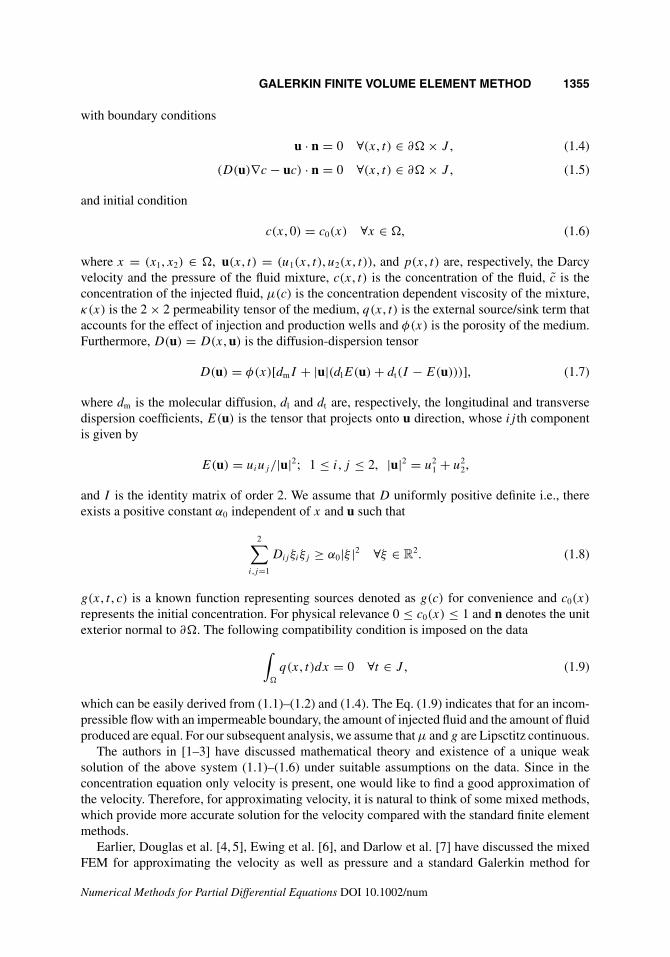
We expect that the advantages of DGFEM over standard FEM should apply to DGFVEM incomparison with standard FVEM. This can be explained as follows. Because of the discontinuityof the trial functions, the elements in the corresponding dual partition are chosen as in Fig. 2(see Fig. 5 also) so that the number of equations are equal to the number of unknowns. This isadvantageous in comparison with the dual partition of the standard FVEM (see Fig. 3), wherecontinuous piecewise linear functions are used as trial functions. Thus, the localizability of thediscontinuous element and its associated dual partition in the new DGFVEM should provide anadvantage for parallel computing and implementation of adaptive FVEM. Moreover, we also notethat the construction of control volume in mixed FVEM and DGFVEM is similar, whereas theshape of control volume in standard FVEM is different, see Figs. 1–3. This indicates that useof DGFVEM would be computationally less expensive compared with standard FVEM for theapproximation of incompressible miscible problems.
Compared with the conforming FEMs, DG methods are conservative in nature and hence,they preserve the physical conservative properties. Sun et al. [33] applied the mixed FEM forpressure-velocity equation and DGFEM for approximating the concentration. Further, Sun andWheeler [34] applied symmetric and nonsymmetric DG methods for approximation of the con-centration equation by assuming that the velocity is known and time independent. DGFVEM arealso not developed in the literature for the approximation of miscible displacement problems, andhence, an attempt has been made to introduce DGFVEM for approximating the concentrationequation. In this article, we present a mixed FVEM for the approximating the pressure-velocityequations (1.1)–(1.2), (1.4) and a DGFVEM for the approximation of the concentration equation(1.3),(1.5)–(1.6).
This article is organized as follows: In Section II, we discuss the DGFVEM formulation. Theexistence and uniqueness of solution to the discrete problem is discussed in Section III. A priori
Numerical Methods for Partial Differential Equations DOI 10.1002/num

GALERKIN FINITE VOLUME ELEMENT METHOD 1357
FIG. 1. Primal grid Th and dual grid T ∗h . [Color figure can be viewed in the online issue, which is available
at wileyonlinelibrary.com.]
error estimates for velocity, pressure and concentration are presented in Section IV. Finally inSection V, numerical experiments are presented to support our theoretical results.
II. FINITE VOLUME ELEMENT APPROXIMATION
We use a mixed FVEM for the simultaneous approximation of velocity and pressure in (1.1)–(1.2) and a DGFVEM for the approximation of the concentration in (1.3). For this purpose, weintroduce three kinds of grids: one primal grid and two dual grids.
FIG. 2. Dual elements in DGFVEM.
Numerical Methods for Partial Differential Equations DOI 10.1002/num
1358 KUMAR
FIG. 3. Dual elements in standrad FVEM. [Color figure can be viewed in the online issue, which is availableat wileyonlinelibrary.com.]
Let Th = {T } be a regular, quasi-uniform partition of the domain � into closed triangles T ,that is, � = ∪T ∈Th
T . Let hT = diam(T ) and h = maxT ∈ThhT . Let the trial function spaces
Uh and Wh associated with the approximation of velocity and pressure respectively be the lowestorder Raviart-Thomas space for triangles defined by
Uh = {vh ∈ U : vh|T = (a + bx, c + by) ∀T ∈ Th},Wh = {wh ∈ W : wh|T is a constant ∀T ∈ Th},
where U = {v ∈ H(div; �) : v · n = 0 on ∂�}. Let T ∗h denote the dual partition of the primal
grid which consists of interior quadrilaterals and boundary triangles. For the construction of thedual grid T ∗
h , we refer to [15]. In general, let T ∗M denote the dual element corresponding to the
mid-side node M . The union of all the dual elements/control volume elements form a partitionT ∗
h of �. The test space Vh is defined by
Vh = {vh ∈ (L2(�))2 : vh|T ∗M
is a constant vector ∀T ∗M ∈ T ∗
h and vh · n = 0 on ∂�},
where T ∗M denote the dual element corresponding to the mid-side node M . For connecting our
trial and test spaces, we define a transfer operator γh : Uh −→ Vh by
γhvh(x) =Nm∑i=1
vh(Mi)χ∗i (x) ∀x ∈ �, (2.1)
where Nm is the total number of mid-side nodes and χ∗i ’s are the scalar characteristic functions
corresponding to the control volume T ∗Mj
defined by
χ∗i (x) =
{1, if x ∈ T ∗
Mi
0, elsewhere.
Numerical Methods for Partial Differential Equations DOI 10.1002/num

GALERKIN FINITE VOLUME ELEMENT METHOD 1359
FIG. 4. A element V ∗ in the dual partition.
Multiplying (1.1) by γhvh ∈ Vh, integrating over the control volumes T ∗M ∈ T ∗
h , applying theGauss’s divergence theorem and summing up over all the control volumes, we obtain
(κ−1µ(c)u, γhvh) −Nm∑i=1
vh(Mi) ·∫
T ∗Mi
p nT ∗Mi
ds = 0 ∀vh ∈ Uh, (2.2)
where nT ∗Mi
denotes the outward normal vector to the boundary of T ∗Mi
. Set
b(γhvh, wh) = −Nm∑i=1
vh(Mi) ·∫
∂T ∗Mi
wh nT ∗Mi
ds ∀vh ∈ Uh, ∀wh ∈ Wh. (2.3)
Then, the mixed FVE approximation corresponding to (1.1)–(1.2) can be written as: find(uh, ph) : J −→ Uh × Wh such that for t ∈ (0, T ]
(κ−1µ(ch)uh, γhvh) + b(γhvh, ph) = 0 ∀vh ∈ Uh, (2.4)
(∇ · uh, wh) = (q, wh) ∀wh ∈ Wh, (2.5)
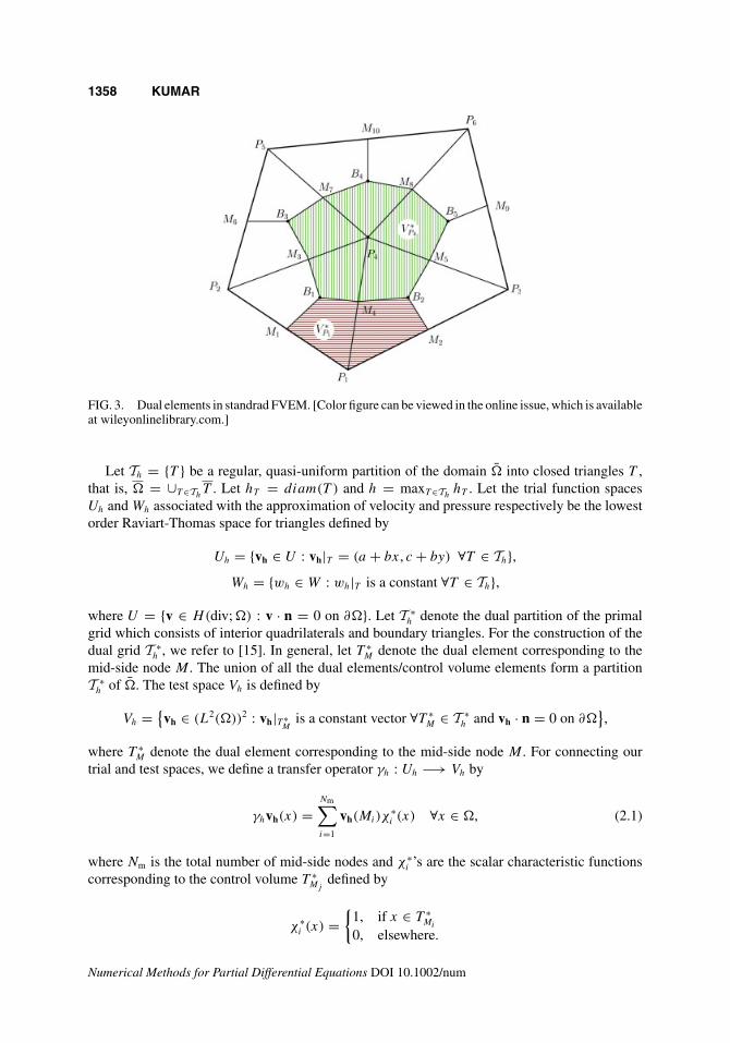
where ch is an DGFVE approximation to c which will be defined in (2.16).We now introduce the dual mesh V∗
h based on Th which will be used in the approximation ofconcentration equation. The dual partition V∗
h corresponding to the primal partition Th is con-structed as follows: Divide each triangle T ∈ Th into three triangles by joining the barycenter B
and the vertices of T as shown is Fig. 2. In general, let V ∗ denote the dual element/control volumein V∗
h , see Fig. 4. The union of these sub-triangles form the dual partition V∗h of �.
We introduce the standard definitions of jumps and averages [29] for scalar and vector func-tions as follows. Let denote the union of all the interior edges of the triangles T of Th. Foran interior edge e shared by two elements T1 and T2, having normal vectors n1 and n2 pointingexterior to T1 and T2 respectively, the average 〈·〉 and jump [·] on e for a scalar q and a vector rare defined, respectively, as:
〈q〉 = 1
2(q1 + q2), [q] = q1n1 + q2n2, 〈r〉 = 1
2(r1 + r2), [r] = r1 · n1 + r2 · n2,
where qi = (q|Ti)|e, ri = (r|Ti
)|e, i = 1, 2.
Numerical Methods for Partial Differential Equations DOI 10.1002/num
1360 KUMAR
In case, e is an edge on ∂�, we define
〈q〉 = q, [q] = qn, 〈r〉 = r, [r] = r · n,
n being the outward normal vector to the boundary ∂�.For applying DGFVEM to approximate the concentration equation, we define the finite
dimensional trial and test spaces Mh and Lh on Th and V∗h , respectively, as
Mh = {vh ∈ L2(�) : vh|T ∈ P1(T ) ∀T ∈ Th
},
Lh = {wh ∈ L2(�) : wh|V ∗ ∈ P0(V∗) ∀V ∗ ∈ V∗
h
},
where Pm(T )( resp. Pm(V ∗)) denotes the polynomials of degree less than or equal to m definedon T (resp. V ∗). Let M(h) = Mh + H 2(�). Define
‖|v‖|2 =∑T ∈Th
|v|21,T +∑e∈
1
he
∫e
[v]2ds, ‖|v‖|1 = ‖|v‖| + ‖v‖, (2.6)
We also define the following discrete norms for φh ∈ Mh as
‖φh‖0,h =∑
T ∈Th
|φh|20,h,T
1/2
, |φh|1,h =∑
T ∈Th
|φh|21,h,T
1/2
, ‖φh‖1,h = (‖φh‖20,h + |φh|21,h
)1/2,
where
|φh|0,h,T ={ |T |
3
(φ2
1 + φ22 + φ2
3
)}1/2
, |φh|1,h,T ={(∣∣∣∣∂φh
∂x
∣∣∣∣2
+∣∣∣∣∂φh
∂y
∣∣∣∣2)
|T |}1/2
, (2.7)
Here |T | is the area of triangle T and φj = φh(Pj ), 1 ≤ j ≤ 3. Further, we also note that ‖ · ‖0,h
and ‖ · ‖1,h are equivalent to ‖ · ‖ and ‖ · ‖1, respectively (see [20, pp. 124]). For connecting thetrial and test spaces, define the operator γ : M(h) −→ Lh as
γ v|V ∗ = 1
he
∫e
v|V ∗ds, V ∗ ∈ V∗h , (2.8)
where “e” is an edge in T and V ∗ is the dual element in V∗h containing e, he being the length of
the edge e (see Fig. 4). We also assume that he and hT are equivalent, i.e., there exist positiveconstants C1 and C2 such that
C1he ≤ hT ≤ C2he. (2.9)
Since γ zh is a constant over each control volume, multiplying (1.3) by γ zh ∈ Lh, integrating,applying the Gauss’s divergence theorem over the control volumes V ∗ ∈ V∗
h and summing upover all control volumes, we obtain(
φ∂c
∂t, γ zh
)−∑
V ∗∈V∗h
∫∂V ∗
(D(u)∇c − uc).nγ zh ds = (g(c), γ zh) ∀zh ∈ Mh, (2.10)
where n denotes the outward unit normal vector to the boundary ∂V ∗ of V ∗.
Numerical Methods for Partial Differential Equations DOI 10.1002/num
GALERKIN FINITE VOLUME ELEMENT METHOD 1361
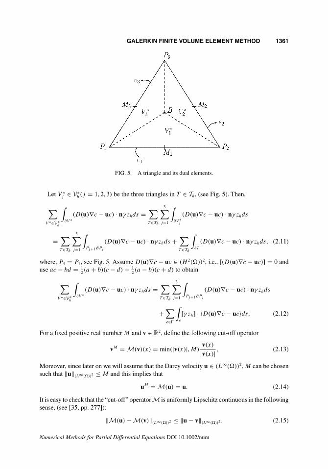
FIG. 5. A triangle and its dual elements.
Let V ∗j ∈ V∗
h(j = 1, 2, 3) be the three triangles in T ∈ Th, (see Fig. 5). Then,
∑V ∗∈V∗
h
∫∂V ∗
(D(u)∇c − uc) · nγ zhds =∑T ∈Th
3∑j=1
∫∂V ∗
j
(D(u)∇c − uc) · nγ zhds
=∑T ∈Th
3∑j=1
∫Pj+1BPj
(D(u)∇c − uc) · nγ zhds +∑T ∈Th
∫∂T
(D(u)∇c − uc) · nγ zhds, (2.11)
where, P4 = P1, see Fig. 5. Assume D(u)∇c − uc ∈ (H 2(�))2, i.e., [(D(u)∇c − uc)] = 0 anduse ac − bd = 1
2 (a + b)(c − d) + 12 (a − b)(c + d) to obtain
∑V ∗∈V∗
h
∫∂V ∗
(D(u)∇c − uc) · nγ zhds =∑T ∈Th
3∑j=1
∫Pj+1BPj
(D(u)∇c − uc) · nγ zhds
+∑e∈
∫e
[γ zh] · 〈D(u)∇c − uc〉ds. (2.12)
For a fixed positive real number M and v ∈ R2, define the following cut-off operator
vM = M(v)(x) = min(|v(x)|, M)v(x)
|v(x)| , (2.13)
Moreover, since later on we will assume that the Darcy velocity u ∈ (L∞(�))2, M can be chosensuch that ‖u‖(L∞(�))2 ≤ M and this implies that
uM = M(u) = u. (2.14)
It is easy to check that the “cut-off” operator M is uniformly Lipschitz continuous in the followingsense, (see [35, pp. 277]):
‖M(u) − M(v)‖(L∞(�))2 ≤ ‖u − v‖(L∞(�))2 . (2.15)
Numerical Methods for Partial Differential Equations DOI 10.1002/num
1362 KUMAR
Now we are in a position to define the DGFVEM formulation for the concentration equation. TheDGFVE scheme corresponding to (1.3) is defined as:
Find ch(t) ∈ Mh such that(φ
∂ch
∂t, γ zh
)+ Ah
(uM
h ; ch, zh
) = (g(ch), γ zh) ∀zh ∈ Mh,
ch(0) = c0,h. (2.16)
Here, uMh is the “cut-off” function of uh defined in (2.13) and c0,h is Ritz projection of c0 to be
defined (4.1) and the bilinear form Ah(v; ·, ·) : M(h) × M(h) −→ R be defined by
Ah(v; φ, ψ) = A1(v; φ, ψ) −∑e∈
∫e
[γψ] · 〈D(v)∇φ − vφ〉ds
−∑e∈
∫e
[γφ] · 〈D(v)∇ψ〉ds +∑e∈
∫e
α
he
[φ] · [ψ]ds ∀v ∈ R2, (2.17)
withA1(v; φ, ψ) = −∑T ∈Th
∑3j=1
∫Pj+1BPj
(D(v)∇φ−vφ)·n γψ ds andα is a penalty parameter
to be defined later. Note that (2.16) is consistent with (2.10), i.e., c also satisfy (2.16).
III. EXISTENCE AND UNIQUENESS OF THE DISCRETE SOLUTION
In this section, we discuss the unique solvability of the system (2.4)–(2.5), (2.16), and for this, weneed to show that the bilinear form Ah(u; ·, ·) satisfies a Gärding type inequality. To demonstratethis, we proceed as follows:
Using Gauss divergence theorem on the control volumes, we write A1(u, ·, ·) as (see, [31, pp.1067]).
A1(u; χ , ψ) =∑T ∈Th
∫T
(D(u)∇χ − uχ) · ∇ψ dx +∑T ∈Th
∫∂T
(D(u)∇χ − uχ) · n)(γψ − ψ)ds
+∑T ∈Th
∫T
∇ · (D(u)∇χ − uχ)(ψ − γψ)ds ∀χ , ψ ∈ M(h). (3.1)
Similarly,
−∑
T
3∑j=1
∫Pj+1BPj
(D(u)∇χ) · nγψ ds =∑T ∈Th
∫T
(D(u)∇χ) · ∇ψ dx
+∑T ∈Th
∫∂T
(D(u)∇χ) · n)(γψ − ψ)ds +∑T ∈Th
∫T
∇ · (D(u)∇χ)(ψ − γψ)ds, (3.2)
Using (3.2) and following the lines of the Lemma 2.1 [31, pp. 1067], we have
−∑T ∈Th
3∑j=1
∫Pj+1BPj
(D(u)∇χh) · nγχh ds ≥ α0
∑T ∈Th
‖∇χh‖2T − C1h‖|χh‖|2. (3.3)
Numerical Methods for Partial Differential Equations DOI 10.1002/num
GALERKIN FINITE VOLUME ELEMENT METHOD 1363
Now, first we find the lower bound for A1(u, ·, ·), and for this, we use the following trace inequality[25, pp. 745].
For w ∈ H 2(T ) and for an edge e of triangle T , we have
‖w‖20,e =
∫e
w2ds ≤ C(h−1
e ‖w‖20,T + he|w|21,T
), (3.4)
Lemma 3.1. If χh ∈ Mh, then
A1(u; χh, χh) ≥ α0
∑T ∈Th
‖∇χh‖2 − C1h‖|χh‖|2 − C2‖χh‖2. (3.5)
Proof. Rewrite A1(u, χh, ψh) as
A1(u, χh, ψh) = −∑T ∈Th
3∑j=1
∫Pj+1BPj
(D(u)∇χh) · n γψh ds
+∑T ∈Th
3∑j=1
∫Pj+1BPj
u · nχh γψh ds. (3.6)
Since γψh is constant on each control volume V ∗, set γψh|V ∗l
= ψl. Using the Cauchy-Schwarzinequality and referring to Fig. 5, we obtain
3∑j=1
∫Pj+1BPj
u · nχh γψh ds =3∑
l=1
∫PlB
u · nlχh(ψl+1 − ψl)ds (ψ4 = ψ1)
≤3∑
l=1
|ψl+1 − ψl|∫
PlB
u · nl χh ds
≤ C
3∑l=1
|ψl+1 − ψl|∫
PlB
χh ds.
A use of the trace inequality (3.4) yields
3∑j=1
∫Pj+1BPj
u · nχhγψh ds ≤ C
3∑l=1
|ψl+1 − ψl| ‖χh‖L2(PlB)(meas(PlB))1/2
≤ C
3∑l=1
|ψl+1 − ψl| ‖χh‖L2(PlB)h1/2T
≤ Ch1/2T
3∑l=1
|ψl+1 − ψl|[h
−1/2T ‖χh‖T + h
1/2T ‖∇χh‖T
](3.7)
Now using Taylor series expansion and (2.7), we find that
|ψl+1 − ψl| ≤ hT
[∣∣∣∣∂ψh
∂x
∣∣∣∣+∣∣∣∣∂ψh
∂y
∣∣∣∣]
≤[(∣∣∣∣∂ψh
∂x
∣∣∣∣2
+∣∣∣∣∂ψh
∂y
∣∣∣∣2)
h2T
]1/2
≤ C|ψh|1,h,T , l = 1, 2, 3. (3.8)
Numerical Methods for Partial Differential Equations DOI 10.1002/num
1364 KUMAR
Substituting (3.8) in (3.7), we arrive at
3∑j=1
∫Pj+1BPj
u · nχh γψh ds ≤ C|ψh|1,h,T [‖χh‖T + hT ‖∇χh‖T ]. (3.9)
Taking summation over all the triangles T ∈ Th, we obtain
∑T ∈Th
3∑j=1
∫Pj+1BPj
u · nχh γψh ds ≤ C‖|ψh‖|(‖χh‖ + h‖|χh‖|). (3.10)
The desire result follows by substituting (3.3) and (3.10) in (3.6) and using Young’s inequality.
Next, we show that the bilinear form Ah(u; ·, ·) satisfies a Gärding type inequality.
Lemma 3.2. There exist positive constants C and C3 independent of h such that for α largeenough, h small enough and v ∈ (L∞(�))2,
Ah(v; φh, φh) ≥ C‖|φh‖|2 − C3‖φh‖2 ∀φh ∈ Mh. (3.11)
Proof. Using the Cauchy-Schwarz inequality and the trace inequality (3.4), we arrive at
∑e∈
∫e
[γφh] · 〈D(u)∇ψh〉ds ≤(∑
e∈
h−1e
∫e
[γφh]2ds
)1/2 (∑e∈
he
∫e
〈D(u)∇ψh〉2ds
)1/2
≤ C
(∑e∈
[γφh]2e
)1/2
‖|ψh‖|.
Now using (2.8) and the Cauchy-Schwarz inequality, we obtain
[γφh]2e =
(1
he
∫e
[φh]ds
)2
≤(
1
he
)2 ∫e
[φh]2ds
∫e
ds =∫
e
1
he
[φh]2ds. (3.12)
This implies that
∑e∈
∫e
[γφh] · 〈D(u)∇ψh〉ds ≤ C
(∑e∈
1
he
∫e
[φh]2ds
)1/2
‖|ψh‖|, (3.13)
and similarly,
∑e∈
∫e
[γφh] · 〈(D(u)∇ψh − uψh〉ds ≤ C
(∑e∈
1
he
∫e
[φh]2ds
)1/2
(‖|ψh‖| + ‖ψh‖). (3.14)
We recall the following well-known inequality ([25, pp. 744])
‖φ‖ ≤ C‖|φ‖| ∀φ ∈ M(h). (3.15)
Numerical Methods for Partial Differential Equations DOI 10.1002/num

GALERKIN FINITE VOLUME ELEMENT METHOD 1365
Now a use of (3.5), (3.13), (3.14), and (3.15) yields
Ah(v; φh, φh) ≥ α0
∑T ∈Th
‖∇φh‖2 − C1h‖|φh‖|2 − C2‖φh‖2 − C‖|φh‖|(∑
e∈
1
he
∫e
[φh]2ds
)1/2
+ α∑e∈
1
he
∫e
[φh]2ds.
A use of Young’s inequality yields
Ah(v; φh, φh) ≥ α0
∑T ∈Th
‖∇φh‖2 − C1h‖|φh‖|2 − C2‖φh‖2 − C2
2α0
(∑e∈
1
he
∫e
[φh]2ds
)
− α0
2‖|φh‖|2 + α
∑e∈
1
he
∫e
[φh]2ds
≥ α0
2
∑T ∈Th
‖∇φh‖2 − C1h‖|φh‖|2 − C2‖φh‖2 +(
α − C2
2α0− α0
2
)∑e∈
1
he
∫e
[φh]2ds
≥ C(α)‖|φh‖|2 − C3‖φh‖2 − C1h‖|φh‖|2 ≥ C‖|φh‖|2 − C3‖φh‖2,
where C(α) = min(
α02 , α − C2
2α0− α0
2
)and α0 is as in (1.8). Here, we have to choose the
parameter α such that the term(α − C2
2α0− α0
2
)is positive and h small enough such that
C = C(α) − C1h > 0.
Now, the uniqueness of the solution of (2.4)–(2.5), (2.16) can be shown as follows:For a given ch, the existence and uniqueness of the discrete solution uh and ph can be shown by
using the saddle point formulation techniques. Since uMh is the cut-off function of uh, the existence
of uh implies the existence of uMh . To show the existence and uniqueness of the concentration in
(2.16), we argue as follows. On substituting (uMh (ch)) in (2.16), we obtain a system of nonlinear
ordinary differential equations in ch. Using Picard’s theorem, there exists a unique solution ch in(0, th) for some 0 < th ≤ T . To continue the solution for all t ∈ J , we need an a priori boundfor ch.
Now, we state the following lemma without proof, which can be shown by using the propertiesof the operator γ and the arguments used in the Lemma 4.1.2 given in [20, pp. 192].
Lemma 3.3. For φh, ψh ∈ Mh,
(φh, γψh) = (ψh, γφh). (3.16)
Moreover, there exist positive constants C1 and C2, independent of h such that
C1‖φh‖ ≤ ‖|φh‖|h ≤ C2‖φh‖ ∀φh ∈ Mh, (3.17)
and
‖γφh‖ ≤ C‖φh‖ ∀φh ∈ Mh. (3.18)
Numerical Methods for Partial Differential Equations DOI 10.1002/num
1366 KUMAR
Now, choosing zh = ch in (2.16) and using (3.16), we obtain
1
2
d
dt(φch, γ ch) + Ah
(uM
h ; ch, ch
) ≤ |(g(ch), γ ch)| (3.19)
Using the Cauchy-Schwarz inequality and (3.18), we obtain
|(g(ch), γ ch)| ≤ C(‖ch‖2 + ‖c‖2). (3.20)
Substituting (3.11) and (3.20) in (3.19), we arrive at
1
2
d
dt(φch, γ ch) + C2‖|ch‖|2 ≤ C3(‖ch‖2 + ‖c‖2). (3.21)
Integrating from 0 to T and using (3.17), we obtain
‖ch‖2 +∫ T
0‖|ch‖|2ds ≤ C
(‖ch(0)‖2 +
∫ T
0‖ch‖2ds +
∫ T
0‖c‖2ds
)(3.22)
A use of Gronwall’s lemma in (3.22) gives an a priori estimate in L2-norm for all ch. Now the apriori bound ‖ch‖L∞(L2) can be used to continue the solution ch for all t ∈ J .
IV. ERROR ESTIMATES
In this section, we discuss the error estimates for the concentration. We write c − ch =(c − Rhc) + (Rhc − ch), where Rh : H 1(�) −→ Mh be the projection of c defined by
B(u; c − Rhc, χh) = 0 ∀χh ∈ Mh. (4.1)
Here, B(u; ψ , χh) = Ah(u; ψ , χh) + (λψ , χh) ∀χh ∈ Mh. Since Ah(u; χh, χh) ≥ C‖|χh‖|2 −C2‖χh‖2, choose λ with λ ≥ C2, then B(u; χh, χh) is coercive in the norm ‖| · ‖|1, i.e., there existsa positive constant C independent of h such that
B(u; χh, χh) ≥ C‖|χh‖|21 ∀χh ∈ Mh. (4.2)
Below, in a series of lemmas we establish estimates of c − Rhc. For this, we need the followingexisting results, which will also be used in the subsequent analysis.
Let Ihc ∈ Mh be an interpolant of c, which has the following approximation properties [36]:
|c − Ihc|s,T ≤ Ch2−sT ‖c‖2,T ∀T ∈ Th, s = 0, 1, 2. (4.3)
Moreover, if φ ∈ W 2,∞(�), then
‖φ − Ihφ‖1,∞ ≤ Ch‖φ‖2,∞. (4.4)
Furthermore, we need the following inverse inequalities (see [36, pp. 141]):
‖χ‖1,∞ ≤ Ch−1‖χ‖1 ∀χ ∈ Mh, (4.5)
Numerical Methods for Partial Differential Equations DOI 10.1002/num

GALERKIN FINITE VOLUME ELEMENT METHOD 1367
and
‖χ‖1 ≤ Ch−1‖χ‖ ∀χ ∈ Mh. (4.6)
By usual interpolation theory, for χ ∈ H 1(T ), we have (see [36]):
‖χ − γχ‖T ≤ Ch‖∇χ‖T . (4.7)
Using the properties of γ operator it is easy to see that, for T ∈ Th and φh ∈ Mh following holdstrue ([32, pp. 1409])
∫T
(φh − γφh) dx = 0 and∫
∂T
(φh − γφh) ds = 0 (4.8)
Let fT be the average value of f over the triangle T . Then using (4.8), the Cauchy-Schwarzinequality and (4.7), we find that
∫T
f (ψh − γψh)dx =∫
T
(f − fT )(ψh − γψh)dx
≤ ‖f − fT ‖T ‖ψh − γψh‖T ≤ Ch2‖∇f ‖T ‖∇ψh‖T . (4.9)
To obtain the bounds for c −Rhc in ‖| · ‖|1 norm, we need to show that the bilinear form Ah(u; ·, ·)is bounded with respect to the ‖| · ‖| norm.
Lemma 4.1. For φ, ψ ∈ M(h), there exists a positive constant C such that
|Ah(u; φ, ψ)| ≤ C
‖|φ‖| +
∑
T ∈Th
h2T |φ|2,T
1/2 ‖|ψ‖|
+‖|ψ‖| +
∑
T ∈Th
h2T |ψ |2,T
1/2 ‖|φ‖|
. (4.10)
Proof. Rewrite Ah(u; φ, ψ) = A1h(u; φ, ψ) + A2
h(u; φ, ψ),where
A1h(u; φ, ψ) = −
∑T ∈Th
3∑j=1
∫Pj+1BPj
(D(u)∇φ) · nγψ ds −∑e∈
∫e
[γψ].〈D(u)∇ψ〉ds
−∑e∈
∫e
[γφ] · 〈D(u)∇ψ〉ds +∑e∈
∫e
α
he
[φh] · [ψ]ds, (4.11)
and A2h(u; φ, ψ) =
∑T ∈Th
3∑j=1
∫Pj+1BPj
uφ · nγψ +∑e∈
∫e
[γψ] · 〈uφ〉ds. (4.12)
Numerical Methods for Partial Differential Equations DOI 10.1002/num

1368 KUMAR
The following bound for A1h(u; φ, ψ) can be obtained by using the same arguments as used in the
demonstration of Lemma 2.4 in [32, pp. 1411]
∣∣A1h(u; φ, ψ)
∣∣ ≤ C
‖|φ‖| +
∑
T ∈Th
h2T |φ|22,T
1/2 ‖|ψ‖|
+(‖|ψ‖| +
∑
T ∈Th
h2T |ψ |22,T
1/2 ‖|φ‖|
.
From (3.10) and (3.12), we note that∣∣∣∣∣∣∑T ∈Th
3∑j=1
∫Pj+1BPj
u · n φ γψ ds
∣∣∣∣∣∣ ≤ C ‖|ψ‖|(‖φ‖ + h‖|φ‖|). (4.13)
∣∣∣∣∣∑e∈
∫e
[γψ] · 〈uφ〉ds
∣∣∣∣∣ ≤ C‖|ψ‖| ‖|φ‖|. (4.14)
Substitute (4.13) and (4.14) in (4.12), to obtain∣∣A2h(u; φ, ψ)
∣∣ ≤ C(‖|φ‖| ‖|ψ‖| + ‖|φ‖| ‖ψ‖). (4.15)
Combining the estimates derived for A1h(u; φ, ψ) and A2
h(u; φ, ψ) with (3.15).
Lemma 4.2. There exists a positive constant C independent of h such that
‖|c − Rhc‖|1 ≤ Ch‖c‖2, (4.16)
Proof. Write c − Rhc = (c − Ihc) + (Ihc − Rhc). Using (4.10), we have
|B(u; ψ , χh)| ≤ C
‖|ψ‖|1 +
∑
T ∈Th
hT |ψ |22,T
1/2 ‖|χh‖|1 + ‖|χh‖|1‖|ψ‖|1
. (4.17)
By the definition of ‖| · ‖|, we obtain
‖|c − Ihc‖|2 = |c − Ihc|21,h +∑e∈
1
he
∫e
[c − Ihc]2ds (4.18)
Using the trace inequality (3.4) and (4.3), we find that
1
he
∫e
[c − Ihc]2eds ≤ C
(h−2
e ‖c − Ihc‖20,T + |c − Ihc|21,T
) ≤ Ch2T ‖c‖2
2,T (4.19)
Use (4.19), (4.18), and (4.3), to arrive at
‖|c − Ihc‖|1 ≤ Ch‖c‖2. (4.20)
Numerical Methods for Partial Differential Equations DOI 10.1002/num

GALERKIN FINITE VOLUME ELEMENT METHOD 1369
Apply coercivity (4.2) and boundedness (4.17) of B(u; ·, ·) with (4.1) to obtain
‖|Ihc − Rhc‖|21 ≤ CB(u; Ihc − Rhc, Ihc − Rhc) ≤ CB(u; Ihc − c, Ihc − Rhc)
≤ C
‖|c − Ihc‖|1 +
∑
T ∈Th
hT |c − Ihc|22,T
1/2 ‖|Rhc − Ihc‖|1
+ ‖|Rhc − Ihc‖|1‖|c − Ihc‖|1 , (4.21)
and hence,
‖|Ihc − Rhc‖|1 ≤ C‖|c − Ihc‖|1. (4.22)
Combine the estimates of (4.20) and (4.22) with the triangle inequality.
For deriving the optimal error estimate in L2 norm, we define A(u; ·, ·) : M(h)×M(h) −→ R
as follows:
A(u; φ, ψ) =∑T ∈Th
∫T
(D(u)∇φ − uφ) · ∇ψ dx −∑e∈
∫e
[ψ] · 〈D(u)∇φ − uφ〉ds
−∑e∈
∫e
[φ] · 〈D(u)∇ψ〉ds +∑e∈
∫e
α
he
[φ] · [ψ]ds. (4.23)
Set εa(u; ψ , χ) = A(u; ψ , χ) − Ah(u; ψ , χ) ∀χ ∈ Mh.Below, we establish an estimate for εa(u; c − Rhc, φh)
Lemma 4.3. There exists a positive constant C such that
|εa(u, c − Rhc, φh)| ≤ Ch2
(‖g‖1 +
∣∣∣∣φ ∂c
∂t
∣∣∣∣1
+ ‖c‖2
+ ‖∇ · u‖1 + ‖u‖(H1(�))2
)‖φh‖1 ∀φh ∈ Mh. (4.24)
Proof. Using the definition of the bilinear forms A(u; ·, ·) and Ah(u; ·, ·), we write
A(u; c − Rhc, φh) − Ah(u; c − Rhc, φh) = I1 + I2 + I3, (4.25)
where
I1 =∑T ∈Th
∫T
(D(u)∇(c − Rhc) − u(c − Rhc)) · ∇φh dx − A1(u; c − Rhc, φh)
I2 =∑e∈
∫e
[γφh − φh] · 〈D(u)∇(c − Rhc) − u(c − Rhc)〉ds
I3 =∑e∈
∫e
[γ (c − Rhc) − c − Rhc] · 〈D(u)∇φh〉ds
Numerical Methods for Partial Differential Equations DOI 10.1002/num
1370 KUMAR
Using (3.1), we have
|I1| ≤∣∣∣∣∣∣∑T ∈Th
∫∂T
(φh − γφh)(D(u)∇(c − Rhc)) − u(c − Rhc)) · n ds
∣∣∣∣∣∣+∣∣∣∣∣∣∑T ∈Th
∫T
∇ · (D(u)∇(c − Rhc) − u(c − Rhc))(φh − γφh)dx
∣∣∣∣∣∣= |I11| + |I12|, say. (4.26)
Let for any function Z, ZT be a function designed in a piecewise manner such that for any edgee of a triangle T ∈ Th,
ZT (x) = Z(xc), ∀x ∈ e,
and xc is the mid point of e. Then we have
|ZT − Z| ≤ Ch‖Z‖1,∞. (4.27)
Now, following the demonstration of Lemma 3.1 given in [32, pp. 1414], we obtain the followingestimates I11 and I12.
|I11| ≤ Ch2‖φh‖1‖c‖2. (4.28)
|I12| ≤ Ch2
(‖g‖1 +
∥∥∥∥φ ∂c
∂t
∥∥∥∥1
+ ‖c‖2 + ‖∇ · u‖1 + ‖u‖(H1(�))2
)‖φh‖1. (4.29)
Substitute (4.28), (4.29) in (4.26), we obtain the following bound for I1.
|I1| ≤ Ch2
(‖g‖1 +
∥∥∥∥φ ∂c
∂t
∥∥∥∥1
+ ‖c‖2 + ‖∇ · u‖1 + ‖u‖(H1(�))2
)‖φh‖1. (4.30)
To obtain an estimate for I2, we note that
|I2| ≤∣∣∣∣∣∑e∈
∫e
[φh − γφh] · 〈D(u)∇(c − Rhc)〉ds
∣∣∣∣∣+∣∣∣∣∣∑e∈
∫e
[φh − γφh] · 〈u(c − Rhc)〉ds
∣∣∣∣∣= |J1| + |J2|, say. (4.31)
Using the same argument as used in to bound I1, we find the following bound for J1
|J1| ≤ Ch2‖φh‖1‖c‖2. (4.32)
Similarly, we bound J2 as
|J2| =∣∣∣∣∣∑e∈
∫e
[φh − γφh] · 〈u(c − Rhc)〉ds
∣∣∣∣∣ ≤ ‖c‖2
∣∣∣∣∣∑e∈
∫e
[φh − γφh] · 〈u − uT 〉ds
∣∣∣∣∣≤ Ch‖c‖2‖u‖(W∞
1 (�))2
∑e∈
∫e
[φh − γφh]ds ≤ Ch2‖c‖2‖φh‖1. (4.33)
Numerical Methods for Partial Differential Equations DOI 10.1002/num

GALERKIN FINITE VOLUME ELEMENT METHOD 1371
Substituting (4.32) and (4.33) in (4.31), we obtain
|I2| ≤ Ch2‖φh‖1‖c‖2. (4.34)
To bound I3, we rewrite it as
|I3| =∣∣∣∣∣∑e∈
∫e
[(c − Rhc) − γ (c − Rhc)] · 〈(D − DT )∇φh〉ds
∣∣∣∣∣ ,Using Cauchy-Schwarz inequality, (3.4), (4.7), (4.16), and (4.27), we obtain
|I3| ≤ Ch2‖c‖2‖φh‖1. (4.35)
Now, the lemma follows by substituting (4.30), (4.34), and (4.35) in (4.25).
Lemma 4.4. There exists a positive constant C independent of h such that
‖c − Rhc‖ ≤ Ch2
(‖c‖2 + ‖g‖1 +
∥∥∥∥φ ∂c
∂t
∥∥∥∥1
+ ‖∇ · u‖1 + ‖u‖(H1(�))2
). (4.36)
Proof. To obtain an optimal L2 estimate for c−Rhc, we now appeal to Aubin-Nitsche dualityargument. Let ψ ∈ H 2(�) be a solution of the following adjoint problem:
−∇ · (D(u)∇ψ) − u · ∇ψ + λψ = c − Rhc in �, (4.37)
D(u)∇ψ · n = 0 on ∂�, (4.38)
satisfying the following elliptic regularity condition:
‖ψ‖2 ≤ C‖c − Rhc‖. (4.39)
Multiplying (4.37) by c − Rhc and integrating over � and using (4.1), we arrive at
‖c − Rhc‖2 = [A(u; c − Rhc, ψ − ψh) + λ(c − Rhc, ψ − ψh)]
+ εa(u; c − Rhc, ψh) = L1 + L2, say. (4.40)
For L1, use (4.16) to obtain
|L1| = |A(u; c − Rhc, ψ − ψh) + (u · ∇(c − Rhc), ψ − ψh) + λ(c − Rhc, ψ − ψh)|
≤ C
‖|c − Rhc‖|1 +
∑
T ∈Th
hT |c − Rhc|22,T
1/2 ‖|ψ − ψh‖|1
+‖|ψ − ψh‖|1‖|c − Rhc‖|1]
≤ Ch‖c‖2‖|ψ − ψh‖|1. (4.41)
The following bound for L2 follows from Lemma 4.3.
|L2| ≤ Ch2
(‖g‖1 +
∥∥∥∥φ ∂c
∂t
∥∥∥∥1
+ ‖c‖2 + ‖∇ · u‖1 + ‖u‖(H1(�))2
)‖ψh‖1. (4.42)
Numerical Methods for Partial Differential Equations DOI 10.1002/num
1372 KUMAR
Substitute (4.41) and (4.42) in (4.40) to find that
‖c − Rhc‖2 ≤ C
[h‖c‖2‖ψ − ψh‖1 + h2
(‖g‖1 +
∥∥∥∥φ ∂c
∂t
∥∥∥∥1
+ ‖c‖2
+ ‖∇ · u‖1 + ‖u‖(H1(�))2
)‖ψh‖1
]. (4.43)
Now choose ψh = Ihψ in (4.43) and use (4.39) with (4.3) to obtain
‖c − Rhc‖ ≤ Ch2
(‖c‖2 + ‖g‖1 +
∥∥∥∥φ ∂c
∂t
∥∥∥∥1
+ ‖∇ · u‖1 + ‖u‖(H1(�))2
),
and this completes the demonstration.
A. Error Estimates for Velocity
Since concentration depends on the velocity and vice versa, to derive the error estimates for theconcentration, we also need error estimates for the velocity. For elliptic problems, the authors in[15] have derived error estimates for mixed covolume method by using Raviart- Thomas projec-tion and L2 projection. In the similar way, for a given c, the following theorem can be shownalthough the proof is long so we omit it here.
Theorem 4.1. Assume that the triangulation Th is quasi-uniform. Let (u, p) and (uh, ph),respectively, be the solutions of (1.1)–(1.2) and (2.4)–(2.5). Then, there exists a positive constantC, independent of h, but dependent on the bounds of κ−1 and µ such that
‖u − uh‖(L2(�))2 + ‖p − ph‖ ≤ C[‖c − ch‖ + h(‖u‖(H1(�))2 + ‖p‖1)], (4.44)
‖∇ · (u − uh)‖ ≤ Ch‖∇ · u‖1, (4.45)
B. Error Estimates for Concentration: Main Theorem
Theorem 4.2. Let c and ch be the solutions of (1.3) and (2.16), respectively, and letch(0) = c0,h = Rhc(0). Then, for sufficiently small h, there exists a positive constant C(T )
independent of h but dependent on the bounds of κ−1 and µ such that
‖c − ch‖2L∞(J ;L2)
≤ C(T )
[∫ T
0
(h4
(‖g‖2
1 +∥∥∥∥φ ∂c
∂t
∥∥∥∥2
1
+ ‖u‖(H1(�))2 + ‖∇ · u‖1
+ ‖ct‖22 + ‖gt‖2
1 + ‖ut‖(H1(�))2 + ‖∇ · ut‖1 +∥∥∥∥φ ∂2c
∂t2
∥∥∥∥2
1
+ h2(‖c‖2
2 + ‖u‖2(H1(�))2 + ‖p‖2
1
))ds
]. (4.46)
First, we will establish the following lemma, which will be used in the demonstration of themain theorem, i.e., Theorem 4.2.
Numerical Methods for Partial Differential Equations DOI 10.1002/num
GALERKIN FINITE VOLUME ELEMENT METHOD 1373
Lemma 4.5. There exists a positive constant C such that
∣∣Ah(uM ; Rhc, θ) − Ah
(uM
h ; Rhc, θ)∣∣ ≤ C(‖u − uh‖(L2(�))2 + h‖∇ · (u − uh)‖
+ ‖|ρ‖|)‖|θ‖| ∀θ ∈ Mh. (4.47)
Proof. Using the definition of Ah(·; ·, ·), we obtain
∣∣Ah(uM ; Rhc, θ) − Ah
(uM
h ; Rhc, θ)∣∣ =
∣∣∣∣∣∣∑T ∈Th
3∑j=1
∫Pj+1BPj
(D(uM) − D
(uM
h
))∇Rhc · nγ θ ds
∣∣∣∣∣∣+∣∣∣∣∣∑e∈
∫e
[γRhc] · ⟨(D(uM) − D(uM
h
))∇θ⟩ds
∣∣∣∣∣+∣∣∣∣∣∑e∈
∫e
[γ θ ] · ⟨(D(uM) − D(uM
h
))∇Rhc⟩ds
∣∣∣∣∣+∣∣∣∣∣∣∑T ∈Th
3∑j=1
∫Pj+1BPj
(uM − uM
h
)Rhc · n γ θ ds
∣∣∣∣∣∣+∣∣∣∣∣∑e∈
∫e
[γ θ ] · ⟨(uM − uMh
)Rhc⟩ds
∣∣∣∣∣= A1 + A2 + A3 + A4 + A5, say.
To estimate A1, we note that
A1 =∣∣∣∣∣∣∑T ∈Th
3∑j=1
∫Pj+1BPj
(D(uM) − D
(uM
h
))∇Rhc · n γ θ ds
∣∣∣∣∣∣ =∣∣∣∣∣∣∑T ∈Th
KT
∣∣∣∣∣∣ ,
where KT = ∑3j=1
∫Pj+1BPj
(D(uM) − D(uMh ))∇Rhc · n γ θ ds. Since γ θ is constant over each
control volume V ∗, set γ θ |V ∗l
= θl. Referring to Fig. 5, KT can be written as follows:
KT =3∑
l=1
∫PlB
(D(uM) − D
(uM
h
))∇Rhc · nl(θl+1 − θl)ds (θ4 = θ1).
Then using (4.56) and the Cauchy-Schwarz inequality, we obtain
KT ≤3∑
l=1
|θl+1 − θl|∫
PlB
∣∣(D(uM) − D(uM
h
))∇Rhc · nl
∣∣ds
≤ C
3∑l=1
|θl+1 − θl|∥∥D(uM) − D
(uM
h
)∥∥(L2(PlB))2×2(meas(PlB))1/2.
We also note that the matrix D(u) defined in (1.7) is uniformly Lipschitz continuous (see [35, pp.287]), i.e., there exists a constant C such that for u and v ∈ (L2(�))2,
‖D(u) − D(v)‖(L2(�))2×2 ≤ C‖u − v‖(L2(�))2 . (4.48)
Numerical Methods for Partial Differential Equations DOI 10.1002/num

1374 KUMAR
Use (4.48), the trace inequality (3.4) and (2.15) to obtain
KT ≤ C
3∑l=1
|θl+1 − θl|∥∥uM − uM
h
∥∥(L2(PlB))2h
1/2T ≤ C
3∑l=1
|θl+1 − θl| ‖u − uh‖(L2(PlB))2h1/2T
≤ Ch1/2T
3∑l=1
|θl+1 − θl|[h
−1/2T ‖u − uh‖T + h
1/2T ‖∇ · (u − uh)‖T
]. (4.49)
Now using Taylor series expansion and (2.7), for l = 1, 2, 3, we find that
|θl+1 − θl| ≤ hT
[∣∣∣∣∂θ
∂x
∣∣∣∣+∣∣∣∣∂θ
∂y
∣∣∣∣]
≤[(∣∣∣∣∂θ
∂x
∣∣∣∣2
+∣∣∣∣∂θ
∂y
∣∣∣∣2)
h2T
]1/2
≤ C|θ |1,h,T .
Substitute (4.50) in (4.49) to arrive at
KT ≤ C|θ |1,h,T (‖u − uh‖T + hT ‖∇ · (u − uh)‖T ).
With the estimates of KT and using equivalence of the norm ‖ · ‖0, h and ‖φh‖, we obtain
A1 ≤ C(‖u − uh‖(L2(�))2 + h‖∇ · (u − uh)‖)‖|θ‖|. (4.50)
Since [γ c] = 0, we can write
A2 =∣∣∣∣∣∑e∈
∫e
[γRhc] · ⟨(D(uM) − D(uM
h
))∇θ⟩ds
∣∣∣∣∣ (4.51)
≤∣∣∣∣∣∑e∈
∫e
[γρ] · 〈D(uM)∇θ〉ds
∣∣∣∣∣+∣∣∣∣∣∑e∈
∫e
[γρ] · ⟨D(uMh
)∇θ⟩ds
∣∣∣∣∣ . (4.52)
Using the same argument as in deriving (3.13), we obtain
∣∣∣∣∣∑e∈
∫e
[γρ] · 〈D(uM)∇θ〉ds
∣∣∣∣∣ ≤ C‖|ρ‖| ‖|θ‖|, (4.53)
∣∣∣∣∣∑e∈
∫e
[γρ] · ⟨D(uMh
)∇θ⟩ds
∣∣∣∣∣ ≤ C‖|ρ‖| ‖|θ‖|. (4.54)
Substituting (4.53) and (4.54) in (4.51), we obtain
A2 ≤ C‖|ρ‖| ‖|θ‖|. (4.55)
Now, we bound A3 as follows:The following bound for ‖Rhc‖1,∞, can be obtained by using (4.5), (4.4), (4.16), and (4.22)
‖Rhc‖1,∞ ≤ C‖c‖2,∞. (4.56)
Numerical Methods for Partial Differential Equations DOI 10.1002/num

GALERKIN FINITE VOLUME ELEMENT METHOD 1375
Now, using (4.56) and the Cauchy-Schwarz inequality, we obtain
A3 =∣∣∣∣∣∑e∈
∫e
[γ θ ] · ⟨(D(uM) − D(uM
h
))∇Rhc⟩ds
∣∣∣∣∣≤ C
(∑e∈
∫e
[γ θ ]2ds
)1/2 (∑e∈
∥∥D(uM) − D(uM
h
)∥∥2
(L2(e))2×2
)1/2
.
Now using (4.48) and (2.15), we arrive at
A3 ≤ C
(∑e∈
∫e
[γ θ ]2ds
)1/2 (∑e∈
‖u − uh‖2(L2(e))2
)1/2
Using the trace inequality (3.4), we obtain
A3 ≤ C‖|θ‖|(‖u − uh‖(L2(�))2 + h‖∇ · (u − uh)‖). (4.57)
A4 and A5 can be bounded in a similar way as A1 and A3, respectively
A4 + A5 ≤ C‖|θ‖|(‖u − uh‖(L2(�))2 + h‖∇ · (u − uh)‖). (4.58)
The result follows after combining the estimates derived for A1 · · · A5.
Demonstration of the Main Theorem. Write c − ch = (c − Rhc) + (Rhc − ch) = ρ + θ .Since the estimates of ρ are known, we need to find only the estimates of θ .
Multiply (1.3) by γ zh, integrate over �. Then subtract the resulting equation from (2.16) toobtain (
φ∂θ
∂t, γ zh
)+ Ah(uM ; c, zh) − Ah
(uM
h ; ch, zh
) = −(
φ∂ρ
∂t, γ zh
)
+ (g(c) − g(ch), γ zh) ∀zh ∈ Mh. (4.59)
Put zh = θ and use the definition of Rh to obtain(φ
∂θ
∂t, γ θ
)+ Ah(uM
h ; θ , θ) = −(
φ∂ρ
∂t, γ θ
)+ (λρ, θ) + (g(c) − g(ch), γ θ)
− [Ah(uM ; Rhc, θ) − Ah
(uM
h ; Rhc, θ)]
= E1 + E2 + E3 + E4, say. (4.60)
To estimate E1 and E − 2, we use the Cauchy Schwartz inequality, boundedness of φ and (3.18)to obtain
|E1| + |E2| ≤ C
(∥∥∥∥∂ρ
∂t
∥∥∥∥+ ‖ρ‖)
‖θ‖. (4.61)
Since µ and g are Lipschitz continuous, using (3.18), we estimate E3 as
|E3| ≤ |(g(ch) − g(c), γ θ)| ≤ C‖c − ch‖ ‖θ‖. (4.62)
Numerical Methods for Partial Differential Equations DOI 10.1002/num

1376 KUMAR
The bound for E4 follows from Lemma 4.5 and hence,
|E4| ≤ C(‖u − uh‖(L2(�))2 + h‖∇ · (u − uh)‖ + ‖|ρ‖|)‖|θ‖|. (4.63)
Substitute the estimates of E1, · · · , E4 in (4.60) and use (3.11), Young’s inequality, nonsingularityof the function φ with standard kick-back arguments to obtain
d
dt‖|θ‖|2h + (α0 − ε)‖|θ‖|2 ≤ C
[h2‖∇ · (u − uh)‖2 + ‖|ρ‖|2‖u − uh‖2
(L2(�))2
+ ‖c − ch‖2 + ‖ρ‖2 +∥∥∥∥∂ρ
∂t
∥∥∥∥2
+ ‖θ‖2
]. (4.64)
Now, from (4.44), we note that
‖u − uh‖(L2(�))2 ≤ C(‖ρ‖ + ‖θ‖ + h(‖u‖(H1(�))2 + ‖p‖1)). (4.65)
A use of (4.36), (4.65), and (4.45) in (4.64) yields
d
dt‖|θ‖|2h + α1‖|θ‖|2 ≤ C
[h4
(‖g‖2
1 + ‖u‖(H1(�))2 + ‖∇ · u‖1 +∥∥∥∥φ ∂c
∂t
∥∥∥∥2
1
+‖ct‖22 + ‖gt‖2
1 + ‖ut‖(H1(�))2 + ‖∇ · ut‖1 +∥∥∥∥φ ∂2c
∂t2
∥∥∥∥2
1
)
+ h2(‖c‖2
2 + ‖u‖2(H1(�))2 + ‖p‖2
1
)+ ‖θ‖2
]. (4.66)
Since ch(0) = Rhc(0), we have θ(0) = 0. An application of Gronwall’s inequality with (3.17),(4.66) yields
‖θ‖2L∞(J ;L2)
≤ C(T )
[∫ T
0
{h4(‖g‖2
1 + ‖u‖(H1(�))2 + ‖∇ · u‖1
+∥∥∥∥φ ∂c
∂t
∥∥∥∥2
1
+ ‖ct‖22 + ‖gt‖2
1 + ‖ut‖(H1(�))2 + ‖∇ · ut‖1
+∥∥∥∥φ ∂2c
∂t2
∥∥∥∥2
1
)+ h2
(‖c‖22 + ‖u‖2
(H1(�))2 + ‖p‖21
)}ds
]. (4.67)
The theorem follows by applying the triangle inequality.Combining the estimates derived in (4.44) and (4.46), we obtain the following estimates for
the velocity and pressure.
Numerical Methods for Partial Differential Equations DOI 10.1002/num
GALERKIN FINITE VOLUME ELEMENT METHOD 1377
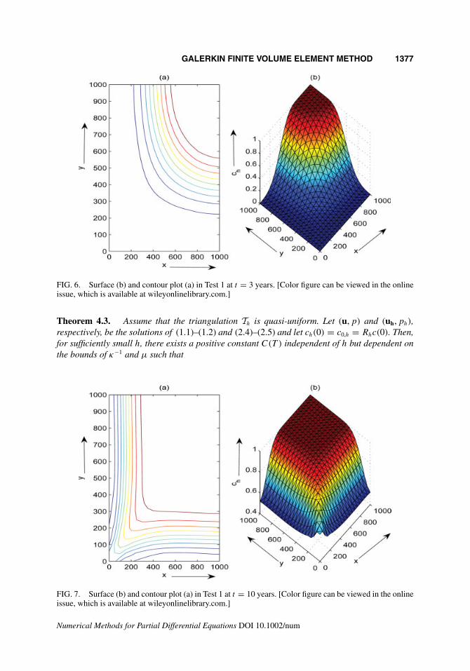
FIG. 6. Surface (b) and contour plot (a) in Test 1 at t = 3 years. [Color figure can be viewed in the onlineissue, which is available at wileyonlinelibrary.com.]
Theorem 4.3. Assume that the triangulation Th is quasi-uniform. Let (u, p) and (uh, ph),respectively, be the solutions of (1.1)–(1.2) and (2.4)–(2.5) and let ch(0) = c0,h = Rhc(0). Then,for sufficiently small h, there exists a positive constant C(T ) independent of h but dependent onthe bounds of κ−1 and µ such that
FIG. 7. Surface (b) and contour plot (a) in Test 1 at t = 10 years. [Color figure can be viewed in the onlineissue, which is available at wileyonlinelibrary.com.]
Numerical Methods for Partial Differential Equations DOI 10.1002/num

1378 KUMAR
FIG. 8. Surface (b) and contour plot (a) in Test 2 at t = 3 years. [Color figure can be viewed in the onlineissue, which is available at wileyonlinelibrary.com.]
‖u − uh‖2L∞(J ;(L2(�))2)
+ ‖p − ph‖2L∞(J ;L2(�))
≤ C(T )
[∫ T
0
{h4
(‖g‖2
1 + ‖u‖(H1(�))2
+‖∇ · u‖1 +∥∥∥∥φ ∂c
∂t
∥∥∥∥2
1
+ ‖ct‖22 + ‖gt‖2
1 + ‖ut‖(H1(�))2 + ‖∇ · ut‖1 +∥∥∥∥φ ∂2c
∂t2
∥∥∥∥2
1
)
+ h2(‖c‖2
2 + ‖u‖2(H1(�))2 + ‖p‖2
1
)}ds
]. (4.68)
V. NUMERICAL EXPERIMENTS
For our numerical experiments, we consider (1.1)–(1.6), with q = q+ − q− and g(x, t , c) =cq+ − cq−, where c is the injection concentration and q+ and q− are the production and injectionrates, respectively.
For the test problems, we have taken the data from [13]. � = (0, 1000) × (0, 1000) ft2 andJ = [0, 3600] days, viscosity of oil is µ(0) = 1.0 cp. The injection well is located at the upper rightcorner (1000, 1000) with the injection rate q+ = 30 ft2/day and injection concentration c = 1.0.The production well is located at the lower left corner with the production rate q− = 30 ft2/dayand c(x, 0) = 0. In the numerical simulation for spatial discretization, we choose in 20 divisionson both x and y axes. For time discretization, we take �tp = 360 days and �tc = 120 days.
Test 1: The permeability κ is 80 and φ = 0.1 and the mobility ratio between the resident andinjected fluid is M = 1. Furthermore, we assume that the molecular diffusion is dm = 1 anddispersion coefficients are zero.
The surface and contour plots for the concentration at t = 3 and t = 10 years are presentedin Figs. 6 and 7, respectively. Because only molecular diffusion is present and viscosity is also
Numerical Methods for Partial Differential Equations DOI 10.1002/num
GALERKIN FINITE VOLUME ELEMENT METHOD 1379
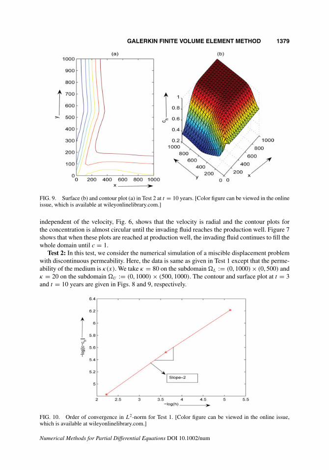
FIG. 9. Surface (b) and contour plot (a) in Test 2 at t = 10 years. [Color figure can be viewed in the onlineissue, which is available at wileyonlinelibrary.com.]
independent of the velocity, Fig. 6, shows that the velocity is radial and the contour plots forthe concentration is almost circular until the invading fluid reaches the production well. Figure 7shows that when these plots are reached at production well, the invading fluid continues to fill thewhole domain until c = 1.
Test 2: In this test, we consider the numerical simulation of a miscible displacement problemwith discontinuous permeability. Here, the data is same as given in Test 1 except that the perme-ability of the medium is κ(x). We take κ = 80 on the subdomain �L := (0, 1000) × (0, 500) andκ = 20 on the subdomain �U := (0, 1000) × (500, 1000). The contour and surface plot at t = 3and t = 10 years are given in Figs. 8 and 9, respectively.
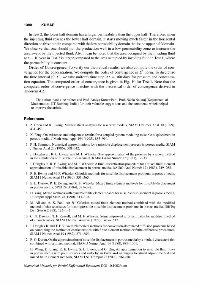
FIG. 10. Order of convergence in L2-norm for Test 1. [Color figure can be viewed in the online issue,which is available at wileyonlinelibrary.com.]
Numerical Methods for Partial Differential Equations DOI 10.1002/num
1380 KUMAR
In Test 2, the lower half domain has a larger permeability than the upper half. Therefore, whenthe injecting fluid reaches the lower half domain, it starts moving much faster in the horizontaldirection on this domain compared with the low permeability domain that is the upper half domain.We observe that one should put the production well in a low permeability zone to increase thearea swept by the injected fluid. Also it can be noted that the area occupied by the invading fluidat t = 10 year in Test 2 is larger compared to the area occupied by invading fluid in Test 1, wherethe permeability is constant.
Order of Convergence: To verify our theoretical results, we also compute the order of con-vergence for the concentration. We compute the order of convergence in L2 norm. To discretizethe time interval [0, T ], we take uniform time step �t = 360 days for pressure and concentra-tion equation. The computed order of convergence is given in Fig. 10 for Test 1. Note that thecomputed order of convergence matches with the theoretical order of convergence derived inTheorem 4.2.
The author thanks the referee and Prof. Amiya Kumar Pani, Prof. Neela Nataraj (Department ofMathematics, IIT Bombay, India) for their valuable suggestions and the comments which helpedto improve the article.
References
1. Z. Chen and R. Ewing, Mathematical analysis for reservoir models, SIAM J Numer Anal 30 (1999),431–453.
2. X. Feng, On existence and uniqueness results for a coupled system modeling miscible displacement inporous media, J Math Anal Appl 194 (1995), 883–910.
3. P. H. Sammon, Numerical approximations for a miscible displacement process in porous media, SIAMJ Numer Anal 23 (1986), 508–542.
4. J. Douglas Jr., R. E. Ewing, and M. F. Wheeler, The approximation of the pressure by a mixed methodin the simulation of miscible displacement, RAIRO Anal Numér 17 (1983), 17–33.
5. J. Douglas Jr., R. E. Ewing, and M. F. Wheeler, A time-discretization procedure for a mixed finite elementapproximation of miscible displacement in porous media, RAIRO Anal Numér 17 (1983), 249–265.
6. R. E. Ewing and M. F. Wheeler, Galerkin methods for miscible displacement problems in porous media,SIAM J Numer Anal 17 (1980), 351–365.
7. B. L. Darlow, R. E. Ewing, and M. F. Wheeler, Mixed finite element methods for miscible displacementin porous media, SPEJ 24 (1984), 391–398.
8. D. Yang, Mixed methods with dynamic finite element spaces for miscible displacement in porous media,J Comput Appl Math 30 (1990), 313–328.
9. M. Ali and A. K. Pani, An H 1-Galerkin mixed finite element method combined with the modifiedmethod of characteristics for incompressible miscible displacement problems in porous media, Diff EqDyn Syst 6 (1998), 135–147.
10. C. N. Dawson, T. F. Russell, and M. F. Wheeler, Some improved error estimates for modified methodof characteristics, SIAM J Numer Anal 26 (1989), 1487–1512.
11. J. Douglas Jr. and T. F. Russell, Numerical methods for convection-dominated diffusion problems basedon combining the method of characteristics with finite element method or finite difference procedures,SIAM J Numer Anal 19 (1982), 871–885.
12. R. G. Duran, On the approximation of miscible displacement in porous media by a method characteristicscombined with a mixed method, SIAM J Numer Anal 14 (1988), 989–1001.
13. H. Wang, D. Liang, R. E. Ewing, S. L. Lyons, and G. Qin, An approximation to miscible fluid flowsin porous media with point sources and sinks by an Eulerian-Lagrangian localized adjoint method andmixed finite element methods, SIAM J Sci Comput 22 (2000), 561–581.
Numerical Methods for Partial Differential Equations DOI 10.1002/num

GALERKIN FINITE VOLUME ELEMENT METHOD 1381
14. S. H. Chou and D. Y. Kwak, Mixed covolume methods on rectangular grids for elliptic problems, SIAMJ Numer Anal 37 (2000), 758–771.
15. S. H. Chou, D. Y. Kwak, and P. Vassilevski, Mixed covolume methods for elliptic problems on triangulargrids, SIAM J Numer Anal 35 (1998), 1850–1861.
16. R. E. Bank and D. J. Rose, Some error estimates for the box method, SIAM J Numer Anal 24 (1987),777–787.
17. Z. Cai, On the finite volume element method, Numer Math 58 (1991), 713–735.
18. P. Chatzipantelidis, Finite volume methods for elliptic PDE’s: a new approach, M2AN Math ModelNumer Anal 36 (2002), 307–324.
19. P. Chatzipantelidis, A finite volume method based on the crouzeix-raviart element for elleptic pdes intwo dimensions, Numer Math 82 (1999), 409–432.
20. R. H. Li, Z. Y. Chen, and W. Wu, Generalized difference methods for differential equations, MarcelDekker, New York, 2000.
21. R. E. Ewing, T. Lin, and Y. Lin, On the accuracy of the finite volume element method based on piecewiselinear polynomials, SIAM J Numer Anal 6 (2002), 1865–1888.
22. S. H. Chou and Q. Li, Error estimates in L2, H 1 and L∞ in covolume methods for elliptic and parabolicproblems: a unified approach, Math Comput 69 (2000), 103–120.
23. S. Kumar, N. Nataraj, and A. K. Pani, Finite volume element method for second order hyperbolicequations, Int J Numer Anal Model 5 (2008), 132–151.
24. I. D. Mishev, Finite volume and finite volume element methods for non-symmetric problems, Ph.D The-sis, Technical Report ISC-96-04-MATH, Institute of Scientific Computation, Texas A&M University,College Station, TX, 1997.
25. D. N. Arnold, An interior penalty finite element method with discontinuous elements, SIAM J NumerAnal 19 (1982), 742–760.
26. I. Babuška, The finite element method with penalty, Math Comput 27 (1973), 221–228.
27. J. Douglas Jr. and T. Dupont, Interior penalty procedures for elliptic and parabolic Galerkin meth-ods, Computing Methods in Applied Sciences, Lecture Notes in Physics, 58, Springer-Verlag, 1976,pp. 207–216.
28. M. F. Wheeler, An elliptic collocation-finite element method with interior penalties, SIAM J NumerAnal 15 (1978), 152–161.
29. D. N. Arnold, F. Brezzi, B. Cockburn, and L. D. Marini, Unified analysis of discontinuous Galerkinmethods for elliptic problems, SIAM J Numer Anal 39 (2002), 1749–1779.
30. S. H. Chou and X. Ye, Unified analysis of finite volume methods for second order elliptic problems,SIAM J Numer Anal 45 (2007), 1639–1653.
31. X. Ye, A new discontinuous finite volume method for elliptic problems, SIAM J Numer Anal 42 (2004),1062–1072.
32. S. Kumar, N. Nataraj, and A. K. Pani, Discontinuous Galerkin finite volume element methods for secondorder linear elliptic problems, Numer Methods Partial Differential Equations 25 (2009), 1402–1424.
33. S. Sun, B. Rivière, and M. F. Wheeler, A combined mixed finite element and discontinuous Galerkinmethod for miscible displacement problem in porous media, Recent progress in Computational AppliedPDEs, Kluwer Acadmic Publishers, Plenum Press, New York, 2002.
34. S. Sun and M. F. Wheeler, Symmetric and nonsymmetric discontinuous Galerkin methods for reactivetransport in porous media, SIAM J Numer Anal 43 (2005), 195–219.
35. S. Sun and M. F. Wheeler, Discontinuous galerkin methods for coupled flow and reactive transportproblems, Appl Numer Math 52 (2005), 273–298.
36. P. G. Ciarlet, The finite element method for elliptic problems, North-Holland, New York, 1978.
Numerical Methods for Partial Differential Equations DOI 10.1002/num


![FUNKTIONALANALYSIS UND GEOMATHEMATIK · [1] M. J. FENGLER: Vector Spherical Harmonic and Vector Wavelet Based Non-Linear Galerkin Schemes for Solving the Incompressible Navier-Stokes](https://static.fdocuments.in/doc/165x107/5ebfec4a97389926ad05ea2f/funktionalanalysis-und-geomathematik-1-m-j-fengler-vector-spherical-harmonic.jpg)