A mini course on percolation theory - Matematiska …steif/perc.pdf · 2010-10-12 · A mini course...

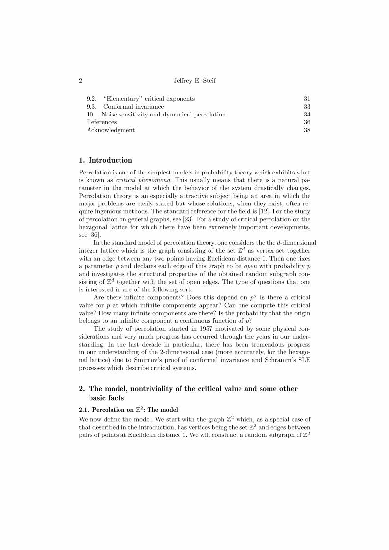
A mini course on percolation theory

Jeffrey E. Steif

Abstract. These are lecture notes based on a mini course on percolation whichwas given at the Jyvaskyla summer school in mathematics in Jyvaskyla, Fin-land, August 2009. The point of the course was to try to touch on a numberof different topics in percolation in order to give people some feel for the field.These notes follow fairly closely the lectures given in the summer school. How-ever, some topics covered in these notes were not covered in the lectures (suchas continuity of the percolation function above the critical value) while othertopics covered in detail in the lectures are not proved in these notes (such asconformal invariance).

Contents

1. Introduction 22. The model, nontriviality of the critical value and some other basic facts 22.1. Percolation on Z2: The model 22.2. The existence of a nontrivial critical value 52.3. Percolation on Zd 92.4. Elementary properties of the percolation function 93. Uniqueness of the infinite cluster 104. Continuity of the percolation function 135. The critical value for trees: the second moment method 156. Some various tools 166.1. Harris’ inequality 176.2. Margulis-Russo Formula 187. The critical value for Z2 equals 1/2 197.1. Proof of pc(2) = 1/2 assuming RSW 197.2. RSW 247.3. Other approaches. 268. Subexponential decay of the cluster size distribution 289. Conformal invariance and critical exponents 309.1. Critical exponents 30

2 Jeffrey E. Steif

9.2. “Elementary” critical exponents 319.3. Conformal invariance 3310. Noise sensitivity and dynamical percolation 34References 36Acknowledgment 38

1. Introduction

Percolation is one of the simplest models in probability theory which exhibits whatis known as critical phenomena. This usually means that there is a natural pa-rameter in the model at which the behavior of the system drastically changes.Percolation theory is an especially attractive subject being an area in which themajor problems are easily stated but whose solutions, when they exist, often re-quire ingenious methods. The standard reference for the field is [12]. For the studyof percolation on general graphs, see [23]. For a study of critical percolation on thehexagonal lattice for which there have been extremely important developments,see [36].

In the standard model of percolation theory, one considers the the d-dimensionalinteger lattice which is the graph consisting of the set Zd as vertex set togetherwith an edge between any two points having Euclidean distance 1. Then one fixesa parameter p and declares each edge of this graph to be open with probability pand investigates the structural properties of the obtained random subgraph con-sisting of Zd together with the set of open edges. The type of questions that oneis interested in are of the following sort.

Are there infinite components? Does this depend on p? Is there a criticalvalue for p at which infinite components appear? Can one compute this criticalvalue? How many infinite components are there? Is the probability that the originbelongs to an infinite component a continuous function of p?

The study of percolation started in 1957 motivated by some physical con-siderations and very much progress has occurred through the years in our under-standing. In the last decade in particular, there has been tremendous progressin our understanding of the 2-dimensional case (more accurately, for the hexago-nal lattice) due to Smirnov’s proof of conformal invariance and Schramm’s SLEprocesses which describe critical systems.

2. The model, nontriviality of the critical value and some otherbasic facts

2.1. Percolation on Z2: The model

We now define the model. We start with the graph Z2 which, as a special case ofthat described in the introduction, has vertices being the set Z2 and edges betweenpairs of points at Euclidean distance 1. We will construct a random subgraph of Z2

A mini course on percolation theory 3

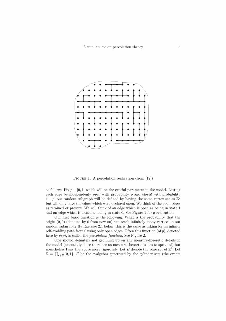
Figure 1. A percolation realization (from [12])

as follows. Fix p ∈ [0, 1] which will be the crucial parameter in the model. Lettingeach edge be independenly open with probability p and closed with probability1 − p, our random subgraph will be defined by having the same vertex set as Z2

but will only have the edges which were declared open. We think of the open edgesas retained or present. We will think of an edge which is open as being in state 1and an edge which is closed as being in state 0. See Figure 1 for a realization.

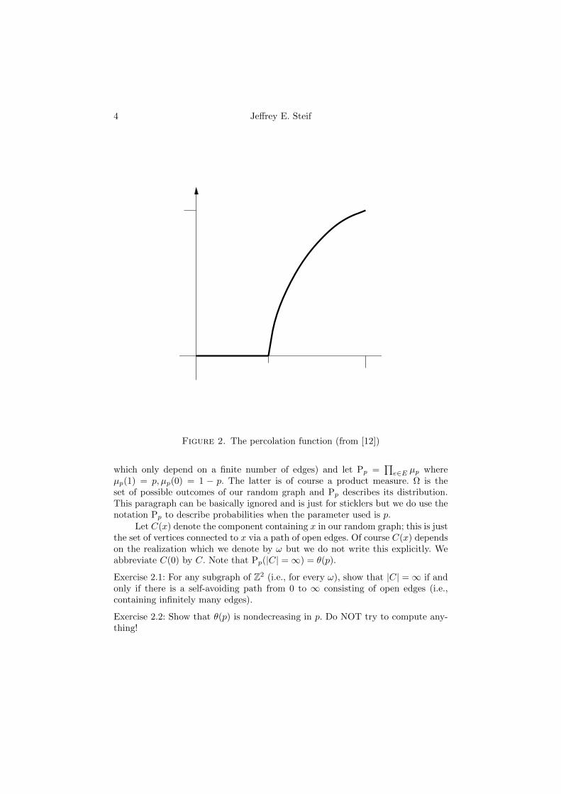
Our first basic question is the following: What is the probability that theorigin (0, 0) (denoted by 0 from now on) can reach infinitely many vertices in ourrandom subgraph? By Exercise 2.1 below, this is the same as asking for an infiniteself-avoiding path from 0 using only open edges. Often this function (of p), denotedhere by θ(p), is called the percolation function. See Figure 2.

One should definitely not get hung up on any measure-theoretic details inthe model (essentially since there are no measure theoretic issues to speak of) butnonetheless I say the above more rigorously. Let E denote the edge set of Z2. LetΩ =

∏e∈E0, 1, F be the σ-algebra generated by the cylinder sets (the events

4 Jeffrey E. Steif

Figure 2. The percolation function (from [12])

which only depend on a finite number of edges) and let Pp =∏e∈E µp where

µp(1) = p, µp(0) = 1 − p. The latter is of course a product measure. Ω is theset of possible outcomes of our random graph and Pp describes its distribution.This paragraph can be basically ignored and is just for sticklers but we do use thenotation Pp to describe probabilities when the parameter used is p.

Let C(x) denote the component containing x in our random graph; this is justthe set of vertices connected to x via a path of open edges. Of course C(x) dependson the realization which we denote by ω but we do not write this explicitly. Weabbreviate C(0) by C. Note that Pp(|C| =∞) = θ(p).

Exercise 2.1: For any subgraph of Z2 (i.e., for every ω), show that |C| =∞ if andonly if there is a self-avoiding path from 0 to ∞ consisting of open edges (i.e.,containing infinitely many edges).

Exercise 2.2: Show that θ(p) is nondecreasing in p. Do NOT try to compute any-thing!


Exercise 2.3: Show that θ(p) cannot be 1 for any p < 1.

2.2. The existence of a nontrivial critical value

The main result in this section is that for p small (but positive) θ(p) = 0 andfor p large (but less than 1) θ(p) > 0. In view of this (and exercise 2.2), thereis a critical value pc ∈ (0, 1) at which the function θ(p) changes from being 0 tobeing positive. This illustrates a so-called phase transition which is a change in theglobal behavior of a system as we move past some critical value. We will see later(see Exercises 2.7 and 2.8) the elementary fact that when θ(p) = 0, a.s. there is noinfinite component anywhere while when θ(p) > 0, there is an infinite componentsomewhere a.s.

Let us finally get to proving our first result. We mention that the method ofproof of the first result is called the first moment method, which just means youbound the probability that some nonnegative integer-valued random variable ispositive by its expected value (which is usually much easier to calculate). In theproof below, we will implicitly apply this first moment method to the number ofself-avoiding paths of length n starting at 0 and for which all the edges of the pathare open.

Theorem 2.1. If p < 1/3, θ(p) = 0.

Proof. : Let Fn be the event that there is a self-avoiding path of length n starting at0 using only open edges. For any given self-avoiding path of length n starting at 0in Z2 (not worrying if the edges are open or not), the probability that all the edgesof this given path are open is pn. The number of such paths is at most 4(3n−1)since there are 4 choices for the first step but at most 3 choices for any later step.This implies that Pp(Fn) ≤ 4(3n−1)pn which → 0 as n → ∞ since p < 1/3. As|C| =∞ ⊆ Fn ∀n, we have that Pp|C| =∞ = 0; i.e., θ(p) = 0.

Theorem 2.2. For p sufficiently close to 1, we have that θ(p) > 0.

Proof. : The method of proof to be used is often called a contour or Peierlsargument, the latter named after the person who proved a phase transition foranother model in statistical mechanics called the Ising model.

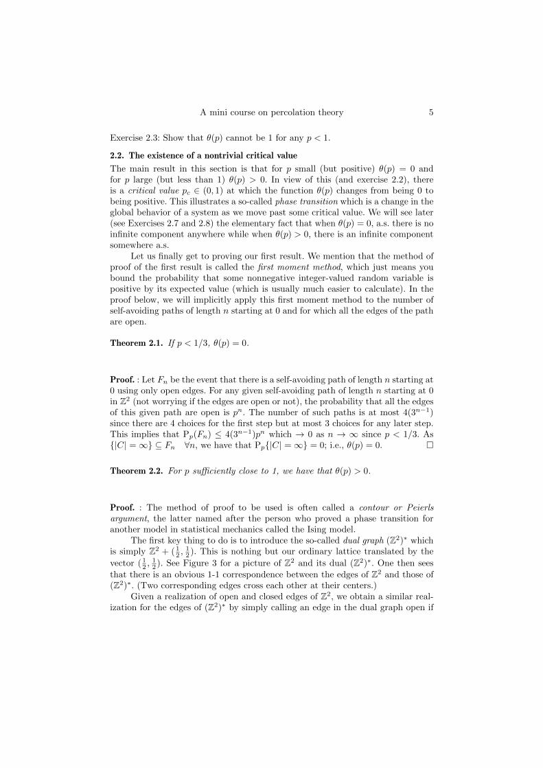
The first key thing to do is to introduce the so-called dual graph (Z2)∗ whichis simply Z2 + ( 1

2 ,12 ). This is nothing but our ordinary lattice translated by the

vector (12 ,

12 ). See Figure 3 for a picture of Z2 and its dual (Z2)∗. One then sees

that there is an obvious 1-1 correspondence between the edges of Z2 and those of(Z2)∗. (Two corresponding edges cross each other at their centers.)

Given a realization of open and closed edges of Z2, we obtain a similar real-ization for the edges of (Z2)∗ by simply calling an edge in the dual graph open if

6 Jeffrey E. Steif

Figure 3. Z2 and its dual (Z2)∗ (from [12])

and only if the corresponding edge in Z2 is open. Observe that if the collection ofopen edges of Z2 is chosen according to Pp (as it is), then the distribution of theset of open edges for (Z2)∗ will trivially also be given by Pp.

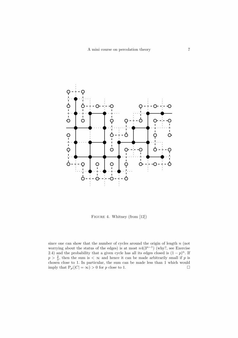
A key step is a result due to Whitney which is pure graph theory. No proofwill be given here but by drawing some pictures, you will convince yourself it isvery believable. Looking at Figures 4 and 5 is also helpful.

Lemma 2.3. |C| < ∞ if and only if ∃ a simple cycle in (Z2)∗ surrounding 0consisting of all closed edges.

Let Gn be the event that there is a simple cycle in (Z2)∗ surrounding 0 havinglength n, all of whose edges are closed. Now, by Lemma 2.3, we have

Pp(|C| <∞) = Pp(∪∞n=4Gn) ≤∞∑n=4

Pp(Gn) ≤∞∑n=4

n4(3n−1)(1− p)n


Figure 4. Whitney (from [12])

since one can show that the number of cycles around the origin of length n (notworrying about the status of the edges) is at most n4(3n−1) (why?, see Exercise2.4) and the probability that a given cycle has all its edges closed is (1 − p)n. Ifp > 2

3 , then the sum is < ∞ and hence it can be made arbitrarily small if p ischosen close to 1. In particular, the sum can be made less than 1 which wouldimply that Pp(|C| =∞) > 0 for p close to 1.

8 Jeffrey E. Steif

Figure 5. Whitney (picture by Vincent Beffara)

Remark:We actually showed that θ(p)→ 1 as p→ 1.

Exercise 2.4: Show that the number of cycles around the origin of length n is atmost n4(3n−1).

Exercise 2.5: Show that θ(p) > 0 for p > 23 .

Hint: Choose N so that∑∞n≥N n4(3n−1)(1− p)n < 1. Let E1 be the event that all

edges are open in [−N,N ]× [−N,N ] and E2 be the event that there are no simplecycles in the dual surrounding [−N,N ]2 consisting of all closed edges. Look nowat E1 ∩ E2.

It is now natural to define the critical value pc by

pc := supp : θ(p) = 0 = infp : θ(p) > 0.

With the help of Exercise 2.5, we have now proved that pc ∈ [1/3, 2/3]. (Themodel would not have been interesting if pc were 0 or 1.) In 1960, Harris [16]proved that θ(1/2) = 0 and the conjecture made at that point was that pc = 1/2and there was indications that this should be true. However, it took 20 more yearsbefore there was a proof and this was done by Kesten [18].

Theorem 2.4. [18] The critical value for Z2 is 1/2.


In Chapter 7, we will give the proof of this very fundamental result.

2.3. Percolation on Zd

The model trivially generalizes to Zd which is the graph whose vertices are theinteger points in Rd with edges between vertices at distance 1. As before, we leteach edge be open with probability p and closed with probability 1−p. Everythingelse is defined identically. We let θd(p) be the probability that there is a self-avoiding open path from the origin to ∞ for this graph when the parameter p isused. The subscript d will often be dropped. The definition of the critical value ind dimensions is clear.

pc(d) := supp : θd(p) = 0 = infp : θd(p) > 0.

In d = 1, it is trivial to check that the critical value is 1 and therefore thingsare not interesting in this case. We saw previously that pc(2) ∈ (0, 1) and it turnsout that for d > 2, pc(d) is also strictly inside the interval (0, 1).

Exercise 2.6: Show that θd+1(p) ≥ θd(p) for all p and d and conclude that pc(d+1) ≤ pc(d). Also find some lower bound on pc(d). How does your lower boundbehave as d→∞?

Exercise 2.7. Using Kolmogorov’s 0-1 law (which says that all tail events haveprobability 0 or 1), show that Pp (some C(x) is infinite) is either 0 or 1. (If youare unfamiliar with Kolmogorov’s 0-1 law, one should say that there are many(relatively easy) theorems in probability theory which guarantee, under certaincircumstances, that a given type of event must have a probability which is either0 or 1 (but they don’t tell which of 0 and 1 it is which is always the hard thing).)

Exercise 2.8. Show that θ(p) > 0 if and only if Pp (some C(x) is infinite)=1.

Nobody expects to ever know what pc(d) is for d ≥ 3 but a much more interestingquestion to ask is what happens at the critical value itself; i.e. is θd(pc(d)) equalto 0 or is it positive. The results mentioned in the previous section imply that itis 0 for d = 2. Interestingly, this is also known to be the case for d ≥ 19 (a highlynontrivial result by Hara and Slade ([15]) but for other d, it is viewed as one ofthe major open questions in the field.

Open question: For Zd, for intermediate dimensions, such as d = 3, is there per-colation at the critical value; i.e., is θd(pc(d)) > 0?

Everyone expects that the answer is no. We will see in the next subsection whyone expects this to be 0.

2.4. Elementary properties of the percolation function

Theorem 2.5. θd(p) is a right continuous function of p on [0, 1]. (This might be agood exercise to attempt before looking at the proof.)

10 Jeffrey E. Steif

Proof. : Let gn(p) := Pp (there is a self-avoiding path of open edges of length nstarting from the origin). gn(p) is a polynomial in p and gn(p) ↓ θ(p) as n→∞.Now a decreasing limit of continuous functions is always upper semi-continuousand a nondecreasing upper semi-continuous function is right continuous.

Exercise 2.9. Why does gn(p) ↓ θ(p) as n → ∞ as claimed in the above proof?Does this convergence hold uniformly in p?

Exercise 2.10. In the previous proof, if you don’t know what words like upper semi-continuous mean (and even if you do), redo the second part of the above proofwith your hands, not using anything.

A much more difficult and deeper result is the following due to van den Berg andKeane ([4]).

Theorem 2.6. θd(p) is continuous on (pc(d), 1].

The proof of this result will be outlined in Section 4. Observe that, given theabove results, we can conclude that there is a jump discontinuity at pc(d) if andonly if θd(pc(d)) > 0. Since nice functions should be continuous, we should believethat θd(pc(d)) = 0.

3. Uniqueness of the infinite cluster

In terms of understanding the global picture of percolation, one of the most naturalquestions to ask, assuming that there is an infinite cluster, is how many infiniteclusters are there?

My understanding is that before this problem was solved, it was not com-pletely clear to people what the answer should be. Note that, for any k ∈ 0, 1, 2, . . . ,∞,it is trivial to find a realization ω for which there are k infinite clusters. (Why?).The following theorem was proved by Aizenman, Kesten and Newman ([1]). Amuch simpler proof of this theorem was found by Burton and Keane ([8]) later onand this later proof is the proof we will follow.

Theorem 3.1. If θ(p) > 0, then Pp(∃ a unique infinite cluster ) = 1.

Before starting the proof, we tell (or remind) the reader of another 0-1 Law whichis different from Kolmogorov’s theorem and whose proof we will not give. I will notstate it in its full generality but only in the context of percolation. (For people whoare familiar with ergodic theory, this is nothing but the statement that a productmeasure is ergodic.)

Lemma 3.2. If an event is translation invariant, then its probability is either 0 or1. (This result very importantly assumes that we are using a product measure, i.e,doing things independently.)


Translation invariance means that you can tell whether the event occurs or notby looking at the percolation realization but not being told where the origin is.For example, the events ‘there exists an infinite cluster’ and ‘there exists at least3 infinite clusters’ are translation invariant while the event ‘|C(0)| =∞’ is not.

Proof of Theorem 3.1. Fix p with θ(p) > 0. We first show that the number ofinfinite clusters is nonrandom, i.e. it is constant a.s. (where the constant maydepend on p). To see this, for any k ∈ 0, 1, 2, . . . ,∞, let Ek be the event that thenumber of infinite cluster is exactly k. Lemma 3.2 implies that Pp(Ek) = 0 or 1 foreach k. Since the Ek’s are disjoint and their union is our whole probability space,there is some k with Pp(Ek) = 1, showing that the number of infinite clusters isa.s. k.

The statement of the theorem is that the k for which Pp(Ek) = 1 is 1 assumingθ(p) > 0; of course if θ(p) = 0, then k is 0. It turns out to be much easier to ruleout all finite k larger than 1 than it is to rule out k = ∞. The easier part, dueto Newman and Schulman ([25]), is stated in the following lemma. Before readingthe proof, the reader is urged to imagine for herself why it would be absurd that,for example, there could be 2 infinite clusters a.s.

Lemma 3.3. For any k ∈ 2, 3, . . ., it cannot be the case that Pp(Ek) = 1.

Proof. : The proof is the same for all k and so we assume that Pp(E5) = 1. LetFM = there are 5 infinite clusters and each intersects [−M,M ]d. Observe that

F1 ⊆ F2 ⊆ . . . ⊆ . . . and ∪iFi = E5. Therefore Pp(Fi)i→∞−→ 1. Choose N so that

Pp(FN ) > 0.

Now, let FN be the event that all infinite clusters touch the boundary of[−N,N ]d. Observe that (1) this event is measurable with respect to the edges

outside of [−N,N ]d and that (2) FN ⊆ FN . Note however that these two events

are not the same. We therefore have that Pp(FN ) > 0. If we let G be the event

that all the edges in [−N,N ]d are open, then G and FN are independent and hence

Pp(G ∩ FN ) > 0. However, it is easy to see that G ∩ FN ⊆ E1 which implies thatPp(E1) > 0 contradicting Pp(E5) = 1.

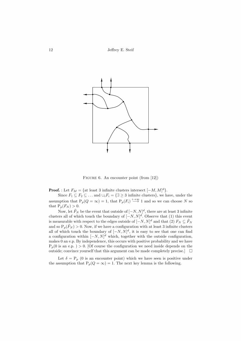
It is much harder to rule out infinitely many infinite clusters, which we donow. This proof is due to Burton and Keane. Let Q be the # of infinite clusters.Assume Pp(Q =∞) = 1 and we will get a contradiction. We call z an “encounterpoint” (e.p.) if

1. z belongs to an infinite cluster C and2. C\z has no finite components and exactly 3 infinite components.

See Figure 6 for how an encounter points looks.

Lemma 3.4. If Pp(Q =∞) = 1, then Pp(0 is an e.p. ) > 0.

12 Jeffrey E. Steif

Figure 6. An encounter point (from [12])

Proof. : Let FM = at least 3 infinite clusters intersect [−M,M ]d.Since F1 ⊆ F2 ⊆ . . . and ∪iFi = ∃ ≥ 3 infinite clusters, we have, under the

assumption that Pp(Q = ∞) = 1, that Pp(Fi)i→∞−→ 1 and so we can choose N so

that Pp(FN ) > 0.

Now, let FN be the event that outside of [−N,N ]d, there are at least 3 infiniteclusters all of which touch the boundary of [−N,N ]d. Observe that (1) this event

is measurable with respect to the edges outside of [−N,N ]d and that (2) FN ⊆ FNand so Pp(FN ) > 0. Now, if we have a configuration with at least 3 infinite clustersall of which touch the boundary of [−N,N ]d, it is easy to see that one can finda configuration within [−N,N ]d which, together with the outside configuration,makes 0 an e.p. By independence, this occurs with positive probability and we havePp(0 is an e.p. ) > 0. [Of course the configuration we need inside depends on theoutside; convince yourself that this argument can be made completely precise.]

Let δ = Pp (0 is an encounter point) which we have seen is positive underthe assumption that Pp(Q =∞) = 1. The next key lemma is the following.


Lemma 3.5. For any configuration and for any N , the number of encounter pointsin [−N,N ]d is at most the number of outer boundary points of [−N,N ]d.

Remark: This is a completely deterministic statement which has nothing to dowith probability.

Before proving it, let’s see how we finish the proof of Theorem 3.1. Choose N solarge that δ(2N + 1)d is strictly larger than the number of outer boundary pointsof [−N,N ]d. Now consider the number of e.p.’s in [−N,N ]d. On the one hand, byLemma 3.5 and the way we chose N , this random variable is always strictly lessthan δ(2N + 1)d. On the other hand, this random variable has an expected valueof δ(2N + 1)d, giving a contradiction.

We are left with the following.

Proof of Lemma 3.5.Observation 1: For any finite set S of encounter points contained in the same

infinite cluster, there is at least one point s in S which is outer in the sense that allthe other points in S are contained in the same infinite cluster after s is removed.To see this, just draw a picture and convince yourself; it is easy.

Observation 2: For any finite set S of encounter points contained in the sameinfinite cluster, if we remove all the elements of S, we break our infinite clusterinto at least |S|+ 2 infinite clusters. This is easily done by induction on |S|. It isclear if |S| = 1. If |S| = k + 1, choose, by observation 1, an outer point s. By theinduction hypothesis, if we remove the points in S\s, we have broken the clusterinto at least k+2 clusters. By drawing a picture, one sees, since s is outer, removalof s will create at least one more infinite cluster yielding k + 3, as desired.

Now fix N and order the infinite clusters touching [−N,N ]d, C1, C2, . . . , Ck,assuming there are k of them. Let j1 be the number of encounter points inside[−N,N ]d which are in C1. Define j2, . . . , jk in the same way. Clearly the number

of encounter points is∑ki=1 ji. Looking at the first cluster, removal of the j1

encounter points which are in [−N,N ]d ∩ C1 leaves (by observation 2 above) atleast j1+2 ≥ j1 infinite clusters. Each of these infinite clusters clearly intersects theouter boundary of [−N,N ]d, denoted by ∂[−N,N ]d. Hence |C1∩∂[−N,N ]d| ≥ j1.Similarly, |Ci ∩ ∂[−N,N ]d| ≥ ji. This yields

|∂[−N,N ]d| ≥k∑i=1

|Ci ∩ ∂[−N,N ]d| ≥k∑i=1

ji.

4. Continuity of the percolation function

The result concerning uniqueness of the infinite cluster that we proved will becrucial in this section (although used in only one point).

14 Jeffrey E. Steif

Proof of Theorem 2.6. Let p > pc. We have already established right continuity andso we need to show that limπp θ(π) = θ(p). The idea is to couple all percolationrealizations, as p varies, on the same probability space. This is not so hard. LetX(e) : e ∈ Ed be a collection of independent random variables indexed by theedges of Zd and having uniform distribution on [0, 1]. We say e ∈ Ed is p-open ifX(e) < p. Let P denote the probability measure on which all of these independentuniform random variables are defined.

Remarks:(i) P(e is p−open ) = p and these events are independent for different e’s. Hence,for any p, the set of e’s which are p-open is just a percolation realization withparameter p. In other words, studying percolation at parameter p is the same asstudying the structure of the p-open edges.(ii) However, as p varies, everything is defined on the same probability space whichwill be crucial for our proof. For example, if p1 < p2, then

e : e is p1 open ⊆ e : e is p2 open.

Now, let Cp be the p-open cluster of the origin (this just means the cluster ofthe origin when we consider edges which are p-open). In view of Remark (ii) above,obviously Cp1 ⊆ Cp2 if p1 < p2 and by Remark (i), for each p, θ(p) = P(|Cp| =∞).Next, note that

limπp

θ(π) = limπp

P(|Cπ| =∞) = P(|Cπ| =∞ for some π < p).

The last equality follows from using countable additivity in our big prob-ability space (one can take π going to p along a sequence). (Note that we haveexpressed the limit that we are interested in as the probability of a certain eventin our big probability space.) Since |Cπ| =∞ for some π < p ⊆ |Cp| =∞, weneed to show that

P(|Cp| =∞\|Cπ| =∞ for some π < p) = 0.

If it is easier to think about, this is the same as saying

P(|Cp| =∞ ∩ |Cπ| <∞ for all π < p) = 0.

Let α be such that pc < α < p. Then a.s. there is an infinite α-open clusterIα (not necessarily containing the origin).

Now, if |Cp| =∞, then, by Theorem 3.1 applied to the p-open edges, we havethat Iα ⊆ Cp a.s. If 0 ∈ Iα, we are of course done with π = α. Otherwise, there isa p-open path ` from the origin to Iα. Let µ = maxX(e) : e ∈ ` which is < p.Now, choosing π such that µ, α < π < p, we have that there is a π open path from0 to Iα and therefore |Cπ| =∞, as we wanted to show.


5. The critical value for trees: the second moment method

Trees, graphs with no cycles, are much easier to analyze than Euclidean latticesand other graphs. Lyons, in the early 90’s, determined the critical value for anytree and also determined whether one percolates or not at the critical value (bothscenarios are possible). See [21] and [22]. Although this was done for general trees,we will stick here to a certain subset of all trees, namely the spherically symmetrictrees, which is still a large enough class to be very interesting.

A spherically symmetric tree is a tree which has a root ρ which has a0 children,each of which has a1 children, etc. So, all vertices in generation k have ak children.

Theorem 5.1. Let An be the number of vertices in the nth generation (which is of

course just∏n−1i=0 ai). Then

pc(T ) = 1/[lim infn

A1/nn ].

Exercise 5.1 (this exercise explains the very important and often used secondmoment method). Recall that the first moment method amounts to using the(trivial) fact that for a nonnegative integer valued random variable X, P(X >0) ≤ E[X].(a). Show that the “converse” of the first moment method is false by showing thatfor nonnegative integer valued random variables X, E[X] can be arbitrarily largewith P(X > 0) arbitrarily small. (This shows that you will never be able to showthat P(X > 0) is of reasonable size based on knowledge of only the first moment.)(b). Show that for any nonnegative random variable X

P(X > 0) ≥ E[X]2

E[X2].

(This says that if the mean is large, then you can conclude that P(X > 0) mightbe “reasonably” large provided you have a reasonably good upper bound on thesecond moment E[X2].) Using the above inequality is called the second momentmethod and it is a very powerful tool in probability.

We will see that the first moment method will be used to obtain a lower bound onpc and the second moment method will be used to obtain an upper bound on pc.

Proof of Theorem 5.1.Assume p < 1/[lim infnA

1/nn ]. This easily yields (an exercise left to the reader)

that Anpn approaches 0 along some subsequence nk. Now, the probability that

there is an open path to level n is at most the expected number of vertices on thenth level connected to the root which is Anp

n. Hence the probability of having anopen path to level nk goes to 0 and hence the root percolates with probability 0.

Therefore pc(T ) ≥ 1/[lim infnA1/nn ].

To show the reverse inequality, we need to show that if p > 1/[lim infnA1/nn ],

then the root percolates with positive probability. Let Xn denote the number

16 Jeffrey E. Steif

of vertices at the nth level connected to the root. By linearity, we know thatE(Xn) = Anp

n. If we can show that for some constant C, we have that for all n,

E(X2n) ≤ CE(Xn)2, (5.1)

we would then have by the second moment method exercise that P(Xn > 0) ≥ 1/Cfor all n. The events Xn > 0 are decreasing and so countable additivity yieldsP(Xn > 0 ∀n) ≥ 1/C. But the latter event is the same as the event that the rootis percolating and one is done.

We now bound the second moment in order to establish (5.1). Letting Uv,wbe the event that both v and w are connected to the root, we have that

E(X2n) =

∑v,w∈Tn

P(Uv,w)

where Tn is the nth level of the tree. Now P(Uv,w) = p2np−kv,w where kv,w is thelevel at which v and w split. For a given v and k, the number of w with kv,w beingk is at most An/Ak. Hence (after a little computation) one gets that the secondmoment above is

≤ Ann∑k=0

p2np−kAn/Ak = E(Xn)2n∑k=0

1/(pkAk).

If∑∞k=0 1/(pkAk) <∞, then we would have (5.1). We have not yet used that p >

1/[lim infnA1/nn ] which we now use. If this holds, then lim infn(pnAn)1/n ≥ 1 + δ

for some δ > 0. This gives that 1/(pkAk) decays exponentially to 0 and we havethe desired convergence of the series.

Remark: The above theorem determines the critical value but doesn’t say whathappens at the critical value. However, the proof gives more than this and some-times tells us what happens even at the critical value. The proof gives that∑∞k=0 1/(pkAk) < ∞ implies percolation at p and in certain cases we might have

convergence of this series at pc giving an interesting case where one percolates atthe critical value. For example if An 2nnα (which means that the ratio of theleft and right sides are bounded away from 0 and ∞ uniformly in n and which ispossible to achieve) then Theorem 5.1 yields pc = 1/2 but furthermore, if α > 1,then

∑nk=0 1/(pkcAk)

∑1/nα <∞ and so we percolate at the critical value. For

α ≤ 1, the above sum diverges and so we don’t know what happens at pc. However,in fact, Lyons showed that

∑nk=0 1/(pkAk) < ∞ is also a necessary condition to

percolate at p. In particular, in the case above with α ≤ 1, we do not percolate atthe critical value. This yields a phase transition in α at a finer scale.

6. Some various tools

In this section, I will state two basic tools in percolation. Although they come upall the time, we have managed to avoid their use until now. However, now we will


need them both for the next section, Section 7, where we give the proof that thecritical value for Z2 is 1/2.

6.1. Harris’ inequality

Harris’ inequality (see [16]) tells us that certain random variables are positivelycorrelated. To state this, we need to first introduce the important property of afunction being increasing. Let Ω := 0, 1J . There is a partial order on Ω given byω ω′ if ωi ≤ ω′i for all i ∈ J .

Definition 6.1. A function f : 0, 1J → R is increasing if ω ω′ implies thatf(ω) ≤ f(ω′). An event is increasing if its indicator function is increasing.

If J is the set of edges in a graph and x and y are vertices, then the eventthat there is an open path from x to y is an increasing event.

Theorem 6.2. Let X := Xii∈J be independent random variables taking values 0and 1. Let f and g be increasing functions as above. Then

E(f(X)g(X)) ≥ E(f(X))E(g(X)).

To understand this, note that an immediate application to percolation is the fol-lowing. Let x, y, z and w be 4 vertices in Zd, A be the event that there is an openpath from x to y and B be the event that there is an open path from z to w. ThenP(A ∩B) ≥ P(A)P(B).

Proof. We do the proof only in the case that J is finite; to go to infinite J is doneby approximation. We prove this by induction on |J |. Assume |J | = 1. Let ω1 andω2 take values 0 or 1. Then since f and g are increasing, we have

(f(ω1)− f(ω2))(g(ω1)− g(ω2)) ≥ 0.

Now letting ω1 and ω2 be independent with distribution X1, one can take expec-tation in the above inequality yielding

E[f(ω1)g(ω1)] + E[f(ω2)g(ω2)]− E[f(ω2)g(ω1)]− E[f(ω1)g(ω2)] ≥ 0.

This says 2E(f(X1)g(X1)) ≥ 2E(f(X1))E(g(X1)).Now assuming it is true for |J | = k − 1 and f and g are functions of k

variables, we have, by the law of total expectation

E(f(X1, . . . , Xk)g(X1, . . . , Xk)) = E[E(f(X1, . . . , Xk)g(X1, . . . , Xk)) | X1, . . . , Xk−1].(6.1)

The k = 1 case implies that for each X1, . . . , Xk−1,

E(f(X1, . . . , Xk)g(X1, . . . , Xk) | X1, . . . , Xk−1) ≥E(f(X1, . . . , Xk) | X1, . . . , Xk−1)E(g(X1, . . . , Xk) | X1, . . . , Xk−1).

Hence (6.1) is

≥ E[E(f(X1, . . . , Xk) | X1, . . . , Xk−1)E(g(X1, . . . , Xk) | X1, . . . , Xk−1)]. (6.2)

18 Jeffrey E. Steif

Now E(f(X1, . . . , Xk) | X1, . . . , Xk−1) and E(g(X1, . . . , Xk) | X1, . . . , Xk−1)are each increasing functions of X1, . . . , Xk−1 as is easily checked and hence theinduction assumption gives that (6.2) is

≥ E[E(f(X1, . . . , Xk) | X1, . . . , Xk−1)]E[E(g(X1, . . . , Xk) | X1, . . . , Xk−1)] =

E(f(X1, . . . , Xk))E(g(X1, . . . , Xk))

and we are done.

Remark: The above theorem is not true for all sets of random variables. Whereprecisely in the above proof did we use the fact that the random variables areindependent?

6.2. Margulis-Russo Formula

This formula has been discovered by a number of people and it describes thederivative with respect to p of the probability under Pp of an increasing event A interms of the very important concept of influence or pivotality. Let Pp be productmeasure on 0, 1J and let A be a subset of 0, 1J which is increasing.

Exercise 6.1. Show that if A is an increasing event, then Pp(A) is nondecreasingin p.

Definition 6.3. Given i ∈ J , and ω ∈ 0, 1J , let ω(i) denote the sequence whichis equal to ω off of i and is 1 on i and ω(i) denote the sequence which is equal to

ω off of i and is 0 on i. Given a (not necessarily increasing) event A of 0, 1J , letPivi(A) be the event, called that ‘i is pivotal for A’, that exactly one of ω(i) andω(i) is in A. Let Ipi (A) = Pp(Pivi(A)), which we call the influence at level p of ion A.

Remarks: The last definition is perhaps a mouth full but contains fundamentallyimportant concepts in probability theory. In words, Pivi(A) is the event that chang-ing the sequence at location i changes whether A occurs. It is an event which ismeasurable with respect to ω off of i. Ipi (A) is then the probability under Pp thatPivi(A) occurs. These concepts are fundamental in a number of different areas,including theoretical computer science.

Exercise 6.2. Let J be a finite set and let A be the event in 0, 1J that there arean even number of 1’s. Determine Pivi(A) and Ipi (A) for each i and p.

Exercise 6.3. Assume that |J | is odd and let A be the event in 0, 1J that there

are more 1’s than 0’s. Describe, for each i, Pivi(A) and I1/2i (A).

The following is the fundamental Margulis-Russo Formula. It was proved indepen-dently in [24] and [27].

Theorem 6.4. Let A be an increasing event in 0, 1J with J a finite set. Then

d(Pp(A))/dp =∑i∈J

Ipi (A).


Exercise 6.4. Let A be the event in 0, 1J corresponding to at least one of thefirst two bits being 1. Verify the Margulis-Russo Formula in this case.

Outline of Proof. Let Yii∈J be i.i.d. uniform variables on [0, 1] and let ωp bedefined by ωpi = 1 if and only if Yi ≤ p. Then Pp(A) = P(ωp ∈ A) and moreoverωp1 ∈ A ⊆ ωp2 ∈ A if p1 ≤ p2. It follows that

Pp+δ(A)− Pp(A) = P(ωp+δ ∈ A\ωp ∈ A).The difference of these two events contains (with a little bit of thought)

∪i∈J (ωp ∈ Pivi(A) ∩ Yi ∈ (p, p+ δ)) (6.3)

and is contained in the union of the latter union (with the open intervals replacedby closed intervals) together with

Yi ∈ [p, p+ δ] for two different i’s.This latter event has probability at most Cδ2 for some constant C (depending

on |J |). Also, the union in (6.3) is disjoint up to an error of at most Cδ2. Hence

Pp+δ(A)−Pp(A) =∑i∈J

P(ωp ∈ Pivi(A)∩Yi ∈ (p, p+δ))+O(δ2) =∑i∈J

Ipi (A)δ+O(δ2).

(Note that we are using here the fact that the event that i is pivotal is measurablewith respect to the other variables.) Divide by δ and let δ → 0 and we are done.

Exercise 6.5. (The square root trick.) Let A1, A2, . . . , An be increasing events withequal probabilities such that P(A1 ∪A2 ∪ . . . An) ≥ p. Show that

P(Ai) ≥ 1− (1− p)1/n.Hint: Use Harris’ inequality.

7. The critical value for Z2 equals 1/2

There are a number of proofs of this result. Here we will stick more or less to theoriginal, following [27]. It however will be a little simpler since we will use onlythe RSW theory (see below) for p = 1/2. The reason for my doing this older proofis that it illustrates a number of important and interesting things.

7.1. Proof of pc(2) = 1/2 assuming RSW

First, L-R will stand for left-right and T-B for top-bottom. Let Jn,m be the eventthat there is a L-R crossing of [0, n] × [0,m]. Let J ′n,m be the event that there isa L-R crossing of [0, n]× (0,m) (i.e., of [0, n]× [1,m− 1]).

Our first lemma explains a very special property for p = 1/2 which alreadyhints that this might be the critical value.

Lemma 7.1. P1/2(Jn+1,n) = 1/2.

20 Jeffrey E. Steif

Proof. This is a symmetry argument using the dual lattice. Let B be the event thatthere is a B-T crossing of [1/2, n+ 1/2]× [−1/2, n+ 1/2] using closed edges in thedual lattice. By a version of Whitney’s theorem, Lemma 2.3, we have that Jn+1,n

occurs if and only if the event B fails. Hence for any p, Pp(Jn+1,n) + Pp(B) = 1.If p = 1/2, we have by symmetry that these two events have the same probabilityand hence each must have probability 1/2.

The next theorem is crucial for this proof and is also crucial in Section 9. It willbe essentially proved in Subsection 7.2. It is called the Russo Seymour Welsh orRSW Theorem and was proved independently in [31] and [26].

Theorem 7.2. For all k, there exists ck so that for all n, we have that

P1/2(Jkn,n) ≥ ck. (7.1)

Remarks: There is in fact a stronger version of this which holds for all p which saysthat if Pp(Jn,n) ≥ τ , then Pp(Jkn,n) ≥ f(τ, k) where f does not depend on n or onp. This stronger version together with (essentially) Lemma 7.1 immediately yieldsTheorem 7.2 above. The proof of this stronger version can be found in [12] butwe will not need this stronger version here. The special case dealing only with thecase p = 1/2 above has a simpler proof due to Smirnov, especially in the context ofthe so-called triangular lattice. (In [6], an alternative simpler proof of the strongerversion of RSW can be found.)

We will now apply Theorem 7.2 to prove that θ(1/2) = 0. This is the first importantstep towards showing pc = 1/2 and was done in 1960 by Harris (although by adifferent method since the RSW Theorem was not available in 1960). As alreadystated, it took 20 more years before Kesten proved pc = 1/2. Before provingθ(1/2) = 0, we first need a lemma which is important in itself.

Lemma 7.3. Let O(`) be the event that there exists an open circuit containing 0 in

Ann(`) := [−3`, 3`]2\[−`, `]2.Then there exists c > 0 so that for all `,

P1/2(O(`)) ≥ c.

Proof. Ann(`) is the (non–disjoint) union of four 6`× 2` rectangles. By Theorem7.2, we know that there is a constant c′ so that for each `, the probability of crossing(in the longer direction) a 6`×2` rectangle is at least c′. By Harris’ inequality, theprobability of crossing each of the 4 rectangles whose union is Ann(`) is at leastc := c′4. However, if we have a crossing of each of these 4 rectangles, we clearlyhave the circuit we are after.

Lemma 7.4. θ(1/2) = 0.


Proof. Let Ck be the event that there is a circuit in Ann(4k) + 1/2 in the duallattice around the origin consisting of closed edges. A picture shows that the Ck’sare independent and Lemma 7.3 implies that P1/2(Ck) ≥ c for all k for somec > 0. It follows that P1/2(Ck i.o. ) = 1 where as usual, Ck i.o. means that thereare infinitely many k so that Ck occurs. However, the latter event implies byLemma 2.3 that the origin does not percolate. Hence θ(1/2) = 0.

The next lemma is very interesting in itself in that it gives a finite criterionwhich implies percolation.

Proposition 7.5. (Finite size criterion) For any p, if there exists an n such that

Pp(J′2n,n) ≥ .98,

then Pp(|C(0)| =∞) > 0.

To prove this proposition, one first establishes

Lemma 7.6. For any ε ≤ .02, if Pp(J′2n,n) ≥ 1− ε, then Pp(J

′4n,2n) ≥ 1− ε/2.

Proof. Let Bn be the event that there exists an L-R crossing of [n, 3n]× (0, n). LetCn be the event that there exists an L-R crossing of [2n, 4n] × (0, n). Let Dn bethe event that there exists a T-B crossing of [n, 2n] × [0, n]. Let En be the eventthat there exists a T-B crossing of [2n, 3n]× [0, n].

We have Pp(Dn) = Pp(En) ≥ Pp(Bn) = Pp(Cn) = Pp(J′2n,n) ≥ 1 − ε.

Therefore Pp(J′2n,n ∩Bn ∩Cn ∩Dn ∩En) ≥ 1− 5ε. By drawing a picture, one sees

that the above intersection of 5 events is contained in J ′4n,n. Letting J ′4n,n denotethe event that exists a L-R crossing of [0, 4n] × (n, 2n), we have that J ′4n,n and

J ′4n,n are independent, each having probability at least 1− 5ε and so

Pp(J′4n,n ∪ J ′4n,n) = 1− (1− Pp(J

′4n,n))2 ≥ 1− 25ε2.

This is at least 1− ε/2 if ε ≤ .02. Since J ′4n,n ∪ J ′4n,n ⊆ J ′4n,2n, we are done.

Proof of Proposition 7.5.Choose n0 such that Pp(J

′2n0,n0

) ≥ .98. Lemma 7.6 and induction implies that forall k ≥ 0

Pp(J′2k+1n0,2kn0

) ≥ 1− .02

2k

and hence ∑k≥0

Pp((J′2k+1n0,2kn0

)c) <∞.

We will define events Hkk≥0 where Hk will be a crossing like J ′2k+1n0,2kn0except

in a different location and perhaps with a different orientation. Let H0 = J ′2n0,n0.

22 Jeffrey E. Steif

Then let H1 be a T-B crossing of (0, 2n0) × [0, 4n0], H2 be a L-R crossing of[0, 8n0] × (0, 4n0), H3 be a T-B crossing of (0, 8n0) × [0, 16n0], etc. Since theprobability of Hk is the same as for J ′2k+1n0,2kn0

, the Borel-Cantelli lemma implies

that a.s. all but finitely many of the Hk’s occur. However, it is clear geometricallythat if all but finitely many of the Hk’s occur, then there is percolation.

Our main theorem in this section is

Theorem 7.7. pc = 1/2.

Before doing the proof, we make a digression and explain how the concept ofa sharp threshold yields the main result as explained in [28]. In order not to losetrack of the argument, this digression will be short and more details concerningthis approach will be discussed in subsection 7.3.

The underlying idea is that increasing events A which ’depend on lots ofrandom variables’ have “sharp thresholds” meaning that the function Pp(A), as pincreases from 0 to 1, goes very sharply from being very small to being very large.

Exercise 7.1. Let A be the event in 0, 1J corresponding to the first bit being a1. Note that Pp(A) = p and hence does not go quickly from 0 to 1 but then againA does not depend on a lot of random variables. Look at what happens if n = |J |is large and A is the event that at least half the random variables are 1.

Definition 7.8. A sequence of increasing events An has a sharp threshold if for allε > 0, there exists N such that for all n ≥ N , there is an interval [a, a+ ε] ⊆ [0, 1](depending on n) such that

Pp(An) < ε for p ≤ aand

Pp(An) > 1− ε for p ≥ a+ ε.

We claim that if the sequence of events J ′2n,n has a sharp threshold, then pc ≤ 1/2.The reason for this is that if pc were 1/2+δ with δ > 0, then, since the probabilityof J ′2n,n at p = 1/2 is not too small due to Theorem 7.2, a sharp threshold wouldtell us that, for large n, Pp(J

′2n,n) would get very large way before p reaches 1/2+δ.

However, Proposition 7.5 would then contradict the definition of the critical value.Slightly more formally, we have the following.

Proof of Theorem 7.7 assuming J ′2n,n has a sharp threshold.First, Lemma 7.4 implies that pc ≥ 1/2. Assume pc = 1/2 + δ0 with δ0 > 0. ThenTheorem 7.2 tells us there is c > 0 such that

P1/2(J ′2n,n) ≥ c

for all n. Let ε = minδ0/2, .02, c. Choose N as given in the definition of asharp threshold and let [a, a + ε] be the corresponding interval for n = N . SinceP1/2(J ′2N,N ) ≥ c ≥ ε, a must be ≤ 1/2. Hence 1/2 + δ0/2 ≥ a+ δ0/2 ≥ a+ ε and


hence P1/2+δ0/2(J ′2N,N ) ≥ 1−ε ≥ .98. By Proposition 7.5, we get P1/2+δ0/2(|C(0)| =∞) > 0, a contradiction.

We now follow Kesten’s proof as modified by Russo ([27]). We even do aslight modification of that so that the stronger version of RSW is avoided; thiswas explained to me by A. Balint.

Proof of Theorem 7.7.Note that Lemma 7.4 implies that pc ≥ 1/2. Assume now that pc = 1/2 + δ0 withδ0 > 0. Let Vn be the number of pivotal edges for the event J4n,n. The key step isthe following proposition.

Proposition 7.9. If pc = 1/2 + δ0 with δ0 > 0, then

limn→∞

infp∈[1/2,1/2+δ0/2]

Ep[Vn] =∞.

Assuming this proposition, the Margulis-Russo formula would then give

limn→∞

infp∈[1/2,1/2+δ0/2]

(d/dp)Pp(J4n,n) =∞.

Since δ0 > 0 by assumption, this of course contradicts the fact that these proba-bilities are bounded above by 1.

Proof of Proposition 7.9.Since J ′4n,n/2 is an increasing event, Theorem 7.2 implies that

infp∈[1/2,1/2+δ0/2],n

Pp(J′4n,n/2) := ε1 > 0.

Next, letting Un be the event that there is a B-T dual crossing of [2n +1/2, 4n− 1/2]× [−1/2, n+ 1/2] consisting of closed edges, we claim that

infp∈[1/2,1/2+δ0/2],n

Pp(Un) := ε2 > 0.

The reason for this is that Pp(Un) is minimized for all n at p = 1/2 + δ0/2,Proposition 7.5 implies that P1/2+δ0/2(J ′2n,n) ≤ .98 for all n since 1/2 + δ0/2 < pc,and the fact that the event J ′2n,n translated to the right distance 2n and Un arecomplementary events.

Now, if Un occurs, let σ be the right-most such crossing. (You need to thinkabout this and convince yourself it is reasonable that, when such a path exists,there exists a right-most path; I would not worry about a precise proof of thiswhich can be topologically quite messy). Since σ is the right-most crossing, giventhe path σ, we know nothing about what happens to the left of σ. (Although youdo not need to know this, it is worth pointing out that this is some complicatedanalogue of what is known as a stopping time and the corresponding strong Markovproperty.) Therefore, conditioned on σ, there is probability at least ε1 that thereis a path of open edges from the left of [0, 4n] × [0, n/2] all the way to 1 step tothe left of σ. Note that if this happens, then there is an edge one step away fromthe end of this path which is pivotal for J4n,n! Let γ be the lowest such path if

24 Jeffrey E. Steif

one exists. Conditioned on both σ and γ, we know nothing about the area to the“top-left” of these curves. Let q be the point where σ and γ meet. For each n,consider the annuli Ann(4k) + 1/2 + q (this is our previous annulus but centeredaround q) but only for those k’s where 4k ≤ n/2. Lemma 7.3 together with thefact that the events O(`) are increasing implies that there is a fixed probabilityε3, independent of n and p ∈ [1/2, 1/2 + δ0/2] and k (with 4k ≤ n/2), such thatwith probability at least ε3, there is an open path from γ to 1 step to the leftof σ running within Ann(4k) + 1/2 + q in this “top-left” area. (For different k’s,these events are independent but this is not needed). Note that each k where thisoccurs gives us a different pivotal edge for the event J4n,n. Since the number ofk’s satisfying 4k ≤ n/2 goes to infinity with n, the proposition is established.

7.2. RSW

In this section, we prove Theorem 7.2. However, it is more convenient to do thisfor site percolation on the triangular lattice or equivalently the hexagonal latticeinstead. (In site percolation, the sites of the graph are independently declared tobe white or black with probability p and one asks for the existence of an infinitepath of white vertices; edges are not removed.)

(The reader will trust us that the result is equally true on Z2 and is welcometo carry out the details.) This simpler proof of RSW for p = 1/2 on the triangularlattice was discovered by Stas Smirnov and can be found in [13] or in [36].

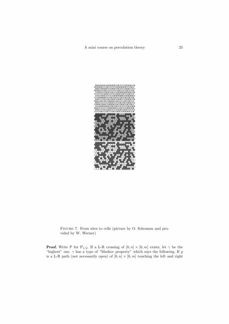
We first quickly define what the triangular lattice and hexagonal lattice are.The set of vertices consists of those points x+ eiπ/3y where x and y are integers.Vertices having distance 1 have an edge between them. See Figure 7 which depictsthe triangular lattice. The triangular lattice is equivalent to the hexagonal latticewhere the vertices of the triangular lattice correspond to the hexagons. Figure7 shows how one moves between these representations. It is somehow easier tovisual the hexagonal lattice compared to the triangular lattice. We mention thatthe duality in Lemma 2.3 is much simpler in this context. For example, there is asequence of white hexagons from the origin out to infinity if and only if there isno path encircling the origin consisting of black hexagons. So, in working with thehexagonal lattice, one does not need to introduce the dual graph as we did for Z2.

Outline of proof of Theorem 7.2 for p = 1/2 for the hexagonal lattice instead. (Wefollow exactly the argument in [36].)

The key step is to prove the following lemma. (The modification for the definitionof Jn,m for the triangular lattice should be pretty clear.)

Lemma 7.10.

P1/2(J2n,m) ≥ (1/4)(P1/2(Jn,m))2.


Figure 7. From sites to cells (picture by O. Schramm and pro-vided by W. Werner)

Proof. Write P for P1/2. If a L-R crossing of [0, n] × [0,m] exists, let γ be the“highest” one. γ has a type of “Markov property” which says the following. If gis a L-R path (not necessarily open) of [0, n] × [0,m] touching the left and right

26 Jeffrey E. Steif

sides only once, then the event γ = g is independent of the percolation process“below” g.

If g is such a L-R path (not necessarily open) of [0, n]× [0,m], let g′ be thereflection of g about x = n (which is then a L-R crossing of [n, 2n]× [0,m]. Assumeg does not touch the x-axis (a similar argument can handle that case as well). Letσ be the part of the boundary of [0, 2n]× [0,m] which is on the left side and belowg (this consists of 2 pieces, the x-axis between 0 and n and the positive y-axisbelow the left point of g). Let σ′ be the reflection of σ about x = n. Symmetryand duality gives that the probability that there is an open path from right belowg to σ′ is 1/2. Call this event A(g).

Observe that if g is a path as above which is open and A(g) occurs, then wehave a path from the left side of [0, 2n]× [0,m] to either the right side of this boxor to the bottom boundary on the right side; call this latter event F . We obtain

P(F ) = P(∪g(F ∩ γ = g)) ≥ P(∪g(A(g) ∩ γ = g)).A(g) and γ = g are independent and we get that the above is therefore

1/2∑g

P(γ = g) = P(Jn,m)/2.

If F ′ is defined to be the reflection about x = n of the event F , then byTheorem 6.2, P(F ∩ F ′) ≥ (1/4)(P(Jn,m))2. Finally, one observes that F ∩ F ′ ⊆J2n,m.

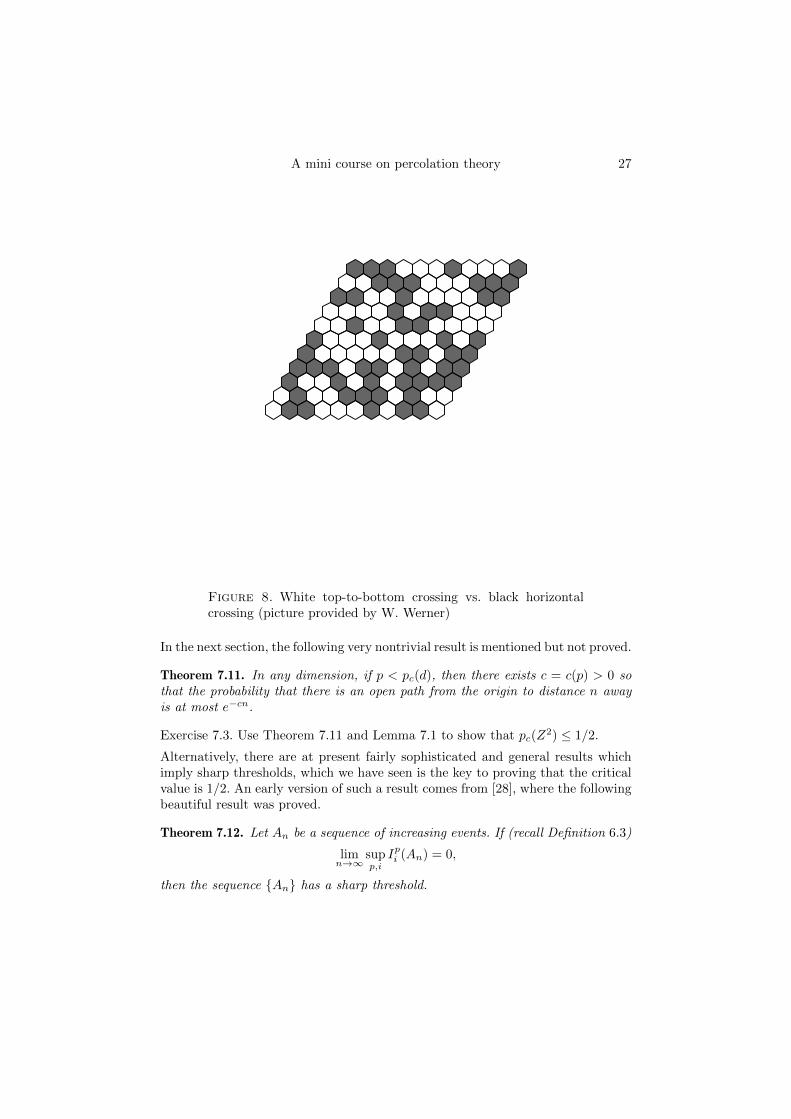
Continuing with the proof, we first note that the analogue of Lemma 7.1for the triangular lattice is that the probability of a crossing of white (or black)hexagons of the 2n× 2n rhombus in Figure 8 is exactly 1/2 for all n. With someelementary geometry, one sees that a crossing of such a rhombus yields a crossingof a n ×

√3n rectangle and hence P(Jn,

√3n) ≥ 1/2 for all n. From here, Lemma

7.10 gives the result by induction.

7.3. Other approaches.

We briefly mention in this section other approaches to computing the critical valueof 1/2.

Exercise 7.2. (Outline of alternative proof due to Yu Zhang for proving θ(1/2) = 0using uniqueness of the infinite cluster; this does not use RSW).

Step 1: Assuming that θ(1/2) > 0, show that the probability that there isan open path from the right side of [−n, n]× [−n, n] to infinity touching this boxonly once (call this event E) approaches 1 as n → ∞. (Hint: Use the square-roottrick of the previous section, Exercise 6.5.)

Step 2: Let F be the event analogous to E but using the left side instead, Gthe analogous event using closed edges in the dual graph and the top of the boxand H the analogous event to G using the bottom of the box. Using step 1, showthat for large n P(E ∩ F ∩G ∩H) > 0.

Step 3: Show how this contradicts uniqueness of the infinite cluster.


Figure 8. White top-to-bottom crossing vs. black horizontalcrossing (picture provided by W. Werner)

In the next section, the following very nontrivial result is mentioned but not proved.

Theorem 7.11. In any dimension, if p < pc(d), then there exists c = c(p) > 0 sothat the probability that there is an open path from the origin to distance n awayis at most e−cn.

Exercise 7.3. Use Theorem 7.11 and Lemma 7.1 to show that pc(Z2) ≤ 1/2.

Alternatively, there are at present fairly sophisticated and general results whichimply sharp thresholds, which we have seen is the key to proving that the criticalvalue is 1/2. An early version of such a result comes from [28], where the followingbeautiful result was proved.

Theorem 7.12. Let An be a sequence of increasing events. If (recall Definition 6.3)

limn→∞

supp,i

Ipi (An) = 0,

then the sequence An has a sharp threshold.

28 Jeffrey E. Steif

Exercise 7.4. Show that limn→∞ supp,i Ipi (J ′2n,n) = 0.

Hint: Use the fact that θ(1/2) = 0. (This exercise together with Theorem 7.12allows us, as we saw after Definition 7.8, to conclude that pc(Z

2) ≤ 1/2.)

Theorem 7.12 is however nontrivial to prove. In [6], the threshold property forcrossings is obtained by a different method. The authors realized that it could bededuced from a sharp threshold result in [10] via a symmetrization argument. Akey element in the proof of the result in [10] is based on [17], where it is shownthat for p = 1/2 if an event on n variables has probability bounded away from 0and 1, then there is a variable of influence at least log(n)/n for this event. (Theproof of this latter very interesting result uses Fourier analysis and the conceptof hypercontractivity). As pointed out in [10], the argument in [17] also yieldsthat if all the influences are small, then the sum of all the influences is very large(provided again that the variance of the event is not too close to 0). A sharpenedversion of this latter fact was also obtained in [35] after [17]. Using this, one canavoid the symmetrization argument mentioned above. One of the big advantagesof the approach in [6] is that it can be applied to other models. In particular, withthe help of the sharp threshold result of [10], it is proved in [7] that the criticalprobability for a model known as Voronoi percolation in the plane is 1/2. It seemsthat at this time neither Theorem 7.12 nor other approaches can achieve this. Thisapproach has also been instrumental for handling certain dependent models.

8. Subexponential decay of the cluster size distribution

Lots of things decay exponentially in percolation when you are away from criticalitybut not everything. I will first explain three objects related to the percolationcluster which do decay exponentially and finally one which does not, which is thepoint of this section. If you prefer, you could skip down to Theorem 8.1 if you onlywant to see the main point of this section.

For our first exponential decay result, it was proved independently by Men-shikov and by Aizenman and Barsky that in any dimension, if p < pc, the prob-ability of a path from the origin to distance n away decays exponentially. Thiswas a highly nontrivial result which had been one of the major open questionsin percolation theory in the 1980’s. It easily implies that the expected size of thecluster of the origin is finite for p < pc.

Exercise 8.1. Prove this last statement.

It had been proved by Aizenman and Newman before this that if the expected sizeof the cluster of the origin is finite at parameter p, then the cluster size has anexponential tail in the sense that

Pp(|C| ≥ n) ≤ e−cn

for all n for some c > 0 where c will depend on p. This does not follow from theMenshikov and Aizenman-Barsky result since that result says that the radius ofthe cluster of the origin decays exponentially while |C| is sort of like the radius


raised to the dth power and random variables who have exponential tails don’tnecessary have the property that their powers also have exponential tails.

The above was all for the subcritical case. In the supercritical case, the radius,conditioned on being finite, also decays exponentially, a result of Chayes, Chayesand Newman. This says that for p > pc,

Pp(An) ≤ e−cn

for all n for some c = c(p) > 0 where An is the event that there is an open pathfrom the origin to distance n away and |C| < ∞. Interestingly, it turns out onthe other hand that the cluster size, conditioned on being finite, does not have anexponential tail in the supercritical regime.

Theorem 8.1. For any p > pc, there exists c = c(p) <∞ so that for all n

Pp(n ≤ |C| <∞) ≥ e−cn(d−1)/d

.

Note that this rules out the possible exponential decay of the tail of the clustersize. (Why?) As can be seen by the proof, the reason for this decay rate is thatit is a surface area effect. Here is the 2 line ’proof’ of this theorem. By a law oflarge numbers type thing (and more precisely an ergodic theorem), the number ofpoints belonging to the infinite cluster in a box with side length n1/d should beabout θ(p)n. However, with probability a fixed constant to the n(d−1)/d, the innerboundary has all edges there while the outer boundary has no edges there whichgives what we want.

Lemma 8.2. Assume that θ(p) > 0. Fix m and let Xm be the number of pointsin Bm := [−m,m]d which belong to the infinite cluster and Fm be the event thatXm ≥ |Bm|θ(p)/2. Then

P(Fm) ≥ θ(p)/2.

Proof. Clearly E(Xm) = |Bm|θ(p). We also have

E(Xm) = E[Xm|Fm]P(Fm) + E[Xm|F cm]P(F cm) ≤ |Bm|P(Fm) + |Bm|θ(p)/2.

Now solve for P(Fm).

Proof of Theorem 8.1.Using the definition of Bm as in the previous lemma, we let F be the event thatthere are at least |Bn1/d |θ(p)/2 points in [0, 2n1/d]d which reach the inner boundary.Let G be the event that all edges between points in the inner boundary are on andlet H be the event that all edges between points in the inner boundary and pointsin the outer boundary are closed. Clearly these three events are independent. Theprobability of F has, by Lemma 8.2, a constant positive probability not depending

on n, and G and H each have probabilty at least e−cn(d−1)/d

for some constant

30 Jeffrey E. Steif

c <∞. The intersection of these three events implies that |Bn1/d |θ(p)/2 ≤ |C| <∞yielding that

Pp(|Bn1/d |θ(p)/2 ≤ |C| <∞) ≥ e−cn(d−1)/d

.

This easily yields the result.

9. Conformal invariance and critical exponents

This section will touch on some very important recent developments in 2 dimen-sional percolation theory that has occurred in the last 10 years. I would not callthis section even an overview since I will only touch on a few things. There is alot to be said here and this section will be somewhat less precise than the earliersections. See [36] for a thorough exposition of these topics.

9.1. Critical exponents

We begin by discussing the concept of critical exponents. We have mentioned inSection 8 that below the critical value, the probability that the origin is connectedto distance n away decays exponentially in n, this being true for any dimension.It had been conjectured for some time that in 2 dimensions, at the critical valueitself, the above probability decays like a power law with a certain power, calleda critical exponent. While this is believed for Z2, it has only been proved for thehexagonal lattice. Recall that one does site percolation rather than bond (edge)percolation on this lattice; in addition, the critical value for this lattice is also 1/2as Kesten also showed.

Let An be the event that there is a white path from the origin to distance naway.

Theorem 9.1. (Lawler, Schramm and Werner, [20]) For the hexagonal lattice, wehave

P1/2(An) = n−5/48+o(1)

where the o(1) is a function of n going to 0 as n→∞.

Remarks: Critical values (such as 1/2 for the Z2 and the hexagonal lattice) arenot considered universal since if you change the lattice in some way the criticalvalue will typically change. However, a critical exponent such as 5/48 is believedto be universal as it is believed that if you take any 2-dimensional lattice and lookat the critical value, then the above event will again decay as the − 5

48 th power ofthe distance.

Exercise 9.1. For Z2, show that there exists c > 0 so that for all n

P1/2(An) ≤ n−c.Hint: Apply Lemma 7.3 to the dual graph.

Exercise 9.2. For Z2, show that for all n

P1/2(An) ≥ (1/4)n−1.


Hint: Use Lemma 7.1.

There are actually an infinite number of other known critical exponents. Let Aknbe the event that there are k disjoint monochromatic paths starting from withindistance (say) 2k of the origin all of which reach distance n from the origin andsuch that at least one of these monochromatic paths is white and at least one is

black. This is referred to as the k-arm event. Let Ak,HR be the analogous event butwhere we restrict to the upper half plane and where the restriction of having atleast one white path and one black path may be dropped. This is referred to asthe half-plane k-arm event.

Theorem 9.2. (Smirnov and Werner, [33]) For the hexagonal lattice, we have

(i) For k ≥ 2, P1/2(Akn) = n−(k2−1)/12+o(1)

(ii) For k ≥ 1, P1/2(Ak,Hn ) = n−k(k+1)/6+o(1) where again the o(1) is a functionof n going to 0 as n→∞.

The proofs of the above results crucially depended on “conformal invariance”,a concept discussed in Section 9.3 and which was proved by Stas Smirnov.

9.2. “Elementary” critical exponents

Computing the exponents in Theorems 9.1 and 9.2 is highly nontrivial and relieson the important concept of conformal invariance to be discussed in the nextsubsection as well as an extremely important development called the Schramm-Lowner evolution. We will not do any of these two proofs; a few special cases ofthem are covered in [36]. (These cases are not the ones which can be done via the“elementary” methods of the present subsection.)

It turns out however that some exponents can be computed by “elementary”means. This section deals with a couple of them via some long exercises. Exercises9.3 and 9.4 below are taken (with permission) (almost) completely verbatim from[36]. In order to do these exercises, we need another important inequality, whichwe managed so far without; this inequality, while arising quite often, is used onlyin this subsection as far as these notes are concerned. It is called the BK inequalitynamed after van den Berg and Kesten; see [5]. The first ingredient is a somewhatsubtle operation on events.

Definition 9.3. Given two events A and B depending on only finitely many edges,we define AB as the event that there are two disjoint sets of edges S and T suchthat the status of edges in S guarantee that A occurs (no matter what the statusof edges outside of S are) and the status of edges in T guarantee that B occurs(no matter what the status of edges outside of T are).

Example: To understand this concept, consider a finite graph G where percolationis being performed, let x, y, z and w be four (not necessarily distinct) vertices, letA be the event that there is an open path from x to y, let B be the event thatthere is an open path from z to w and think about what AB is in this case. Howshould the probability Pp(A B) compare with that of Pp(A)Pp(B)?

32 Jeffrey E. Steif

Theorem 9.4. (van den Berg and Kesten, [5]) (BK inequality).If A and B are increasing events, then Pp(A B) ≤ Pp(A)Pp(B).

While this might seem ’obvious’ in some sense, the proof is certainly non-trivial. When it was proved, it was conjectured to hold for all events A and B.However, it took 12 more years (with false proofs by many people given on theway) before David Reimer proved the above inequality for general events A andB.

Exercise 9.3. Two-arm exponent in the half-plane. Let p = 1/2. Let Λn be theset of hexagons which are of distance at most n from the origin. We considerHn = z ∈ Λn : =(z) ≥ 0 where =(z) is defined to be the imaginary part of thecenter of z. The boundary of Hn can be decomposed into two parts: a horizontalsegment parallel to and close to the real axis and the “angular semi-circle” hn.We say that a point x on the real line is n-good if there exist one open pathoriginating from x and one closed path originating from x + 1, that both stay inx+Hn and join these points to x+ hn (these paths are called “arms”). Note thatthe probability wn that a point x is n-good does not depend on x.

1) We consider percolation in H2n.a) Prove that with a probability that is bounded from below independently ofn, there exists an open cluster O and a closed cluster C, that both intersect thesegment [−n/2, n/2] and h2n, such that C is “to the right” of O.b) Prove that in the above case, the right-most point of the intersection of O withthe real line is n-good.c) Deduce that for some absolute constant c, wn ≥ c/n.

2) We consider percolation in Hn.a) Show that the probability that there exists at least k disjoint open paths joininghn to [−n/2, n/2] in Hn is bounded by λk for some constant λ that does not dependon n (hint: use the BK inequality). Show then that the number K of open clustersthat join hn to [−n/2, n/2] satisfies P(K ≥ k) ≤ λk.b) Show that each 2n-good point in [−n/2, n/2] is the right-most point of theintersection of one of these K clusters with the real line.c) Deduce from this that for some absolute constant c′, (n+ 1)w2n ≤ E(K) ≤ c′.3) Conclude that for some positive absolute constants c1 and c2, c1/n ≤ wn ≤ c2/n.

Exercise 9.4. Three-arm exponent in the half-plane. Let p = 1/2. We say that apoint x is n-Good (mind the capital G) if it is the unique lowest point in x+Hn

of an open cluster C such that C 6⊆ x + Hn. Note that the probability vn that apoint is n-Good does not depend on x.

1) Show that this event corresponds to the existence of three arms, having colorsblack, white and black, originating from the neighborhood of x in x+Hn.

2) Show that the expected number of clusters inside Hn that join hn/2 to hn isbounded. Compare this number of clusters with the number of 2n-Good points inHn/2 and deduce from this that for some constant c1, vn ≤ c1/n2.


3) Show that with probability bounded from below independently of n, thereexists in Hn/2 an n-Good point (note that an argument is needed to show thatwith positive probability, there exists a cluster with a unique lowest point). Deducethat for some positive absolute constant c2, vn ≥ c2/n2.

9.3. Conformal invariance

One of the key steps in proving the above theorems is to prove conformal invarianceof percolation which is itself very important. Before even getting to this, we warmup with posing the following question, which could be thought of in either thecontext of Z2 or the hexagonal lattice.

Question: Letting an be the probability at criticality of having a crossing of [0, 2n]×[0, n], does limn→∞ an exist?

Remark: We have seen in Section 7 that an ≤ 1/2 and that lim inf an > 0.The central limit theorem in probability is a sort of scaling limit. It says

that if you add up many i.i.d. random variables and normalize them properly, youget a nice limiting object (which is the normal distribution). We would like to dosomething vaguely similar with percolation, where the lattice spacing goes to 0 andwe ask if some limiting object emerges. In this regard, note that an is exactly theprobability that there is a crossing of [0, 2]×[0, 1] on the lattice scaled down by 1/n.In studying whether percolation performed on smaller and smaller lattices mighthave some limiting behavior, looking at a crossing of [0, 2]× [0, 1] is one particular(of many) global or macro-events that one may look at. If p is subcritical, thenan goes exponentially to 0, which implies that subcritical percolation on the 1/nscaled down lattice has no interesting limiting behavior.

The conformal invariance conjecture contains 3 ingredients; (i) limits, such asthe sequence an above exist (ii) their values depend only on the ’structure’ of thedomain and hence are conformally invariant and (iii) exact values, due to Cardy,of the values of these limits. We now make this precise.

Let Ω be a bounded simply connected domain of the plane and let A,B,Cand D be 4 points on the boundary of Ω in clockwise order. Scale a 2-dimensionallattice, such as Z2 or the hexagonal lattice T , by 1/n and perform critical per-colation on this scaled lattice. Let P(Ω, A,B,C,D, n) denote that the probabilitythat in the 1/n scaled hexagonal lattice, there is an open path in Ω going from theboundary of Ω between A and B to the boundary of Ω between C and D. (ForZ2, an open path should be interpreted as a path of open edges while for T , itshould be interpreted as a path of white hexagons.) The first half of the followingconjecture is attributed to Michael Aizenman and the second half of the conjectureto John Cardy.

Conjecture 9.5. (i) For all Ω and A,B,C and D as above,

P(Ω, A,B,C,D,∞) := limn→∞

P(Ω, A,B,C,D, n)

exists and is conformally invariant in the sense that if f is a conformal mapping,then P(Ω, A,B,C,D,∞) = P(f(Ω), f(A), f(B), f(C), f(D),∞).

34 Jeffrey E. Steif

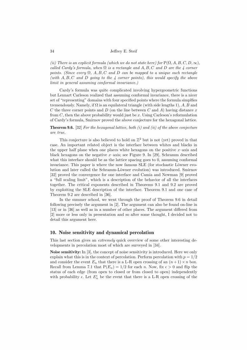
(ii) There is an explicit formula (which we do not state here) for P(Ω, A,B,C,D,∞),called Cardy’s formula, when Ω is a rectangle and A,B,C and D are the 4 cornerpoints. (Since every Ω, A,B,C and D can be mapped to a unique such rectangle(with A,B,C and D going to the 4 corner points), this would specify the abovelimit in general assuming conformal invariance.)

Cardy’s formula was quite complicated involving hypergeometric functionsbut Lennart Carleson realized that assuming conformal invariance, there is a nicerset of “representing” domains with four specified points where the formula simplfiestremendously. Namely, if Ω is an equilateral triangle (with side lengths 1), A,B andC the three corner points and D (on the line between C and A) having distance xfrom C, then the above probability would just be x. Using Carleson’s reformulationof Cardy’s formula, Smirnov proved the above conjecture for the hexagonal lattice.

Theorem 9.6. [32] For the hexagonal lattice, both (i) and (ii) of the above conjectureare true.

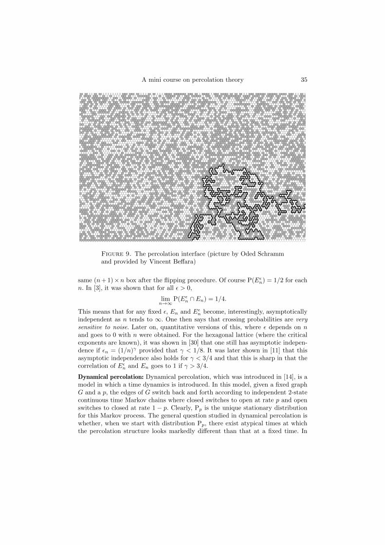
This conjecture is also believed to hold on Z2 but is not (yet) proved in thatcase. An important related object is the interface between whites and blacks inthe upper half plane when one places white hexagons on the positive x–axis andblack hexagons on the negative x–axis; see Figure 9. In [29], Schramm describedwhat this interface should be as the lattice spacing goes to 0, assuming conformalinvariance. This paper is where the now famous SLE (for stochastic Lowner evo-lution and later called the Schramm-Lowner evolution) was introduced. Smirnov[32] proved the convergence for one interface and Camia and Newman [9] proveda “full scaling limit”, which is a description of the behavior of all the interfacestogether. The critical exponents described in Theorems 9.1 and 9.2 are provedby exploiting the SLE description of the interface. Theorem 9.1 and one case ofTheorem 9.2 are described in [36].

In the summer school, we went through the proof of Theorem 9.6 in detailfollowing precisely the argument in [2]. The argument can also be found on-line in[13] or in [36] as well as in a number of other places. The argument differed from[2] more or less only in presentation and so after some thought, I decided not todetail this argument here.

10. Noise sensitivity and dynamical percolation

This last section gives an extremely quick overview of some other interesting de-velopments in percolation most of which are surveyed in [34].

Noise sensitivity: In [3], the concept of noise sensitivity is introduced. Here we onlyexplain what this is in the context of percolation. Perform percolation with p = 1/2and consider the event En that there is a L-R open crossing of an (n+ 1)×n box.Recall from Lemma 7.1 that P(En) = 1/2 for each n. Now, fix ε > 0 and flip thestatus of each edge (from open to closed or from closed to open) independentlywith probability ε. Let Eεn be the event that there is a L-R open crossing of the


Figure 9. The percolation interface (picture by Oded Schrammand provided by Vincent Beffara)

same (n+ 1)×n box after the flipping procedure. Of course P(Eεn) = 1/2 for eachn. In [3], it was shown that for all ε > 0,

limn→∞

P(Eεn ∩ En) = 1/4.

This means that for any fixed ε, En and Eεn become, interestingly, asymptoticallyindependent as n tends to ∞. One then says that crossing probabilities are verysensitive to noise. Later on, quantitative versions of this, where ε depends on nand goes to 0 with n were obtained. For the hexagonal lattice (where the criticalexponents are known), it was shown in [30] that one still has asymptotic indepen-dence if εn = (1/n)γ provided that γ < 1/8. It was later shown in [11] that thisasymptotic independence also holds for γ < 3/4 and that this is sharp in that thecorrelation of Eεn and En goes to 1 if γ > 3/4.

Dynamical percolation: Dynamical percolation, which was introduced in [14], is amodel in which a time dynamics is introduced. In this model, given a fixed graphG and a p, the edges of G switch back and forth according to independent 2-statecontinuous time Markov chains where closed switches to open at rate p and openswitches to closed at rate 1 − p. Clearly, Pp is the unique stationary distributionfor this Markov process. The general question studied in dynamical percolation iswhether, when we start with distribution Pp, there exist atypical times at whichthe percolation structure looks markedly different than that at a fixed time. In

36 Jeffrey E. Steif

almost all cases, the term “markedly different” refers to the existence or nonexis-tence of an infinite connected component. A number of results for this model wereobtained in [14] of which we mention the following.(i) For p less than the critical value, there are no times at which percolation occurswhile for p larger than the critical value, percolation occurs at all times.(ii) There exist graphs which do not percolate at criticality but for which thereexist exceptional times (necessarily of Lebesgue measure 0) at which percolationoccurs.(iii) For large d, there are no exceptional times of percolation for dynamical per-colation run at criticality on Zd. (Recall that we have seen, without proof, thatordinary percolation on Zd for large d does not percolate.) The key property ex-ploited for this result is that the percolation function has a ’finite derivative’ atthe critical value.

It was left open what occurs at Z2 where it is known that the percolationfunction has an ’infinite derivative’ at the critical value. Using the known criticalexponents for the hexagonal lattice, it was proved in [30] that there are in factexceptional times of percolation for this lattice when run at criticality and that theHausdorff dimension of such times is in [1/6, 31/36] with the upper bound beingconjectured. In [11], it was then shown that the upper bound of 31/36 is correctand that even Z2 has exceptional times of percolation at criticality and also thatthis set has positive Hausdorff dimension.

While the relationship between noise sensitivity and dynamical percolation mightnot be clear at first sight, it turns out that there is a strong relation between thembecause the ‘2nd moment calculations’ necessary to carry out a second momentargument for the dynamical percolation model involve terms which are closelyrelated to the correlations considered in the definition of noise sensitivity. See [34]for many more details.

References

[1] Aizenman, M., Kesten, H. and Newman, C. M. Uniqueness of the infinite cluster andcontinuity of connectivity functions for short- and long-range percolation. Comm.Math. Phys. 111, (1987), 505–532.

[2] Beffara, V. Cardy’s formula on the triangular lattice, the easy way. Universality andRenormalization, Vol. 50 of the Fields Institute Communications, (2007), 39–45.

[3] Benjamini, I., Kalai, G. and Schramm, O. Noise sensitivity of Boolean functions and

applications to percolation. Inst. Hautes Etudes Sci. Publ. Math. 90, (1999), 5–43.

[4] van den Berg, J. and Keane, M. On the continuity of the percolation probabilityfunction. Conference in modern analysis and probability (New Haven, Conn., 1982),Contemp. Math. 26, Amer. Math. Soc., Providence, RI, 1984, 61–65.

[5] van den Berg, J. and Kesten, H. Inequalities with applications to percolation andreliability. J. Appl. Probab. 22, (1985), 556–569.


[6] Bollobas B. and Riordan O.M. A short proof of the Harris–Kesten Theorem, Bull.London Math. Soc., 38, (2006), 470–484.

[7] Bollobas B. and Riordan O.M. The critical probability for random Voronoi percolationin the plane is 1/2, Probab. Theory Related Fields, 136, (2006), 417–468.

[8] Burton, R. and Keane, M. Density and uniqueness in percolation. Comm. Math. Phys.121, (1989), 501–505.

[9] Camia, F. and Newman, C. M. Two-dimensional critical percolation: the full scalinglimit, Comm. Math. Phys., 268, (2006), 1–38.

[10] Friedgut, E. and Kalai, G. Every monotone graph property has a sharp threshold,Proc. Amer. Math. Soc., 124, (1996), 2993–3002.

[11] Garban, C., Pete, G. and Schramm, O. The Fourier Spectrum of Critical Percolation,Acta Math., to appear, arXiv:0803.3750[math:PR].

[12] Grimmett, G. Percolation Second edition, Springer-Verlag, (1999), New York.

[13] Grimmett, G. Probability on Graphs, Cambridge University Press, (2010), Cam-bridge.

[14] Haggstrom, O., Peres, Y. and Steif, J. E. Dynamical percolation. Ann. Inst. HenriPoincare, Probab. et Stat. 33, (1997), 497–528.

[15] Hara, T. and Slade, G. (1994) Mean field behavior and the lace expansion, in Prob-ability Theory and Phase Transitions, (ed. G. Grimmett), Proceedings of the NATOASI meeting in Cambridge 1993, Kluwer.

[16] Harris, T. E. A lower bound on the critical probability in a certain percolationprocess. Proc. Cambridge Phil. Soc. 56, (1960), 13–20.

[17] Kahn, J., Kalai, G. and Linial, N. The influence of variables on boolean functions.29th Annual Symposium on Foundations of Computer Science, (1988), 68–80.

[18] Kesten, H. The critical probability of bond percolation on the square lattice equals12. Comm. Math. Phys. 74, (1980), 41–59.

[19] Langlands, R., Pouliot, P. and Saint-Aubin, Y. Conformal invariance in two-dimensional percolation. Bull. Amer. Math. Soc. (N.S.) 30, (1994), 1–61.

[20] Lawler, G., Schramm, O. and Werner, W. One-arm exponent for critical 2D perco-lation. Electron. J. Probab. 7, (2002), no. 2, 13 pp. (electronic).

[21] Lyons, R. Random walks and percolation on trees. Ann. Probab. 18, (1990), 931–958.

[22] Lyons, R. Random walks, capacity, and percolation on trees. Ann. Probab. 20, (1992),2043–2088.

[23] Lyons, R. with Peres, Y. Probability on Trees and Networks. Cambridge UniversityPress. In preparation. Current version available at http://mypage.iu.edu/˜rdlyons/.

[24] Margulis, G. A. Probabilistic characteristics of graphs with large connectivity, Prob-lemy Peredaci Informacii, 10, (1974), 101–108.

[25] Newman, C. M. and Schulman, L. S. Number and density of percolating clusters. J.Phys. A, 14, (1981), 1735–1743.

[26] Russo, L. A note on percolation. Z. Wahrscheinlichkeitstheorie und Verw. Gebiete,43, (1978), 39–48.

[27] Russo, L. On the critical percolation probabilities. Z. Wahrsch. Verw. Gebiete 56,(1981), 229–237.

38 Jeffrey E. Steif

[28] Russo, L. An approximate zero-one law. Z. Wahrsch. Verw. Gebiete 61, (1982), 129–139.

[29] Schramm, O. Scaling limits of loop-erased random walks and uniform spanning trees.Israel J. Math. 118, (2000), 221–288.

[30] Schramm, O. and Steif, J. E. Quantitative noise sensitivity and exceptional timesfor percolation. Ann. Math., 171, (2010), 619–672.

[31] Seymour, P. D. and Welsh, D. J. A. Percolation probabilities on the square lattice.Advances in graph theory (Cambridge Combinatorial Conf., Trinity College, Cam-bridge, 1977). Ann. Discrete Math., 3, (1978), 227–245.

[32] Smirnov, S. Critical percolation in the plane: conformal invariance, Cardy’s formula,scaling limits. C. R. Acad. Sci. Paris Ser. I Math. 333, (2001), 239–244.

[33] Smirnov, S. and Werner, W. Critical exponents for two-dimensional percolation.Math. Res. Lett. 8, (2001), 729–744.

[34] Steif, J. A survey on dynamical percolation. Fractal geometry and stochastics, IV,Birkhauser, (2009), 145–174.

[35] Talagrand, M. On Russo’s approximate zero-one law. Ann. Probab. 22, (1994), 1576–1587.

[36] Werner, W. Lectures on two-dimensional critical percolation. IAS Park City Grad-uate Summer School, 2007, arXiv:0710.0856[math:PR].

Acknowledgment

I would like to thank Andras Balint for explaining to me how one adapts theoriginal proofs of Theorem 7.7 so that one needs only the RSW result for p =1/2. I thank Vincent Beffara for providing me with some pictures. The pictureswhich state in their captions that they have come from reference [12] have beenreproduced courtesy of Geoffrey Grimmett from [12] which I hereby thank. I alsothank the students from the summer school for some of their corrections for thesenotes. Various helpful comments were also given to me by Andras Balint, RagnarFreij and Marcus Warfheimer. I also received useful comments from an anonymousreferee. Lastly, I would like to thank Ville Suomala for organizing the mathematicspart of the Jyvaskyla summer school which was a very enjoyable experience forme.

Jeffrey E. SteifMathematical SciencesChalmers University of TechnologyandMathematical SciencesGoteborg UniversitySE-41296 Gothenburg, Swedene-mail: [email protected]

A mini course on percolation theory - Matematiska …steif/perc.pdf · 2010-10-12 · A mini course...

Documents

Transcript of A mini course on percolation theory - Matematiska …steif/perc.pdf · 2010-10-12 · A mini course...