A Meta-MDP Approach to Explorationfor Lifelong Reinforcement Learning

Francisco M. Garcia and Philip S. ThomasCollege of Information and Computer Sciences

University of Massachusetts AmherstAmherst, MA, USA

{fmgarcia,pthomas}@cs.umass.edu

Abstract

In this paper we consider the problem of how a reinforcement learning agent thatis tasked with solving a sequence of reinforcement learning problems (a sequenceof Markov decision processes) can use knowledge acquired early in its lifetime toimprove its ability to solve new problems. We argue that previous experience withsimilar problems can provide an agent with information about how it should explore

when facing a new but related problem. We show that the search for an optimalexploration strategy can be formulated as a reinforcement learning problem itselfand demonstrate that such strategy can leverage patterns found in the structureof related problems. We conclude with experiments that show the benefits ofoptimizing an exploration strategy using our proposed framework.

1 Introduction

One hallmark of human intelligence is our ability to leverage knowledge collected over our lifetimeswhen we face a new problem. When dealing with a new problem related to one we already know howto address, we leverage the experience obtained from solving the former problem. For example, uponbuying a new car, we do not re-learn from scratch how to drive a car, instead we use the experiencewe had driving a previous car to quickly adapt to the new control and dynamics.

Standard reinforcement learning (RL) methods lack this ability. When faced with a new problem—anew Markov decision process (MDP)—they typically start learning from scratch, initially makinguninformed decisions in order to explore and learn about the current problem they face. The problemof creating agents that can leverage previous experiences to solve new problems is called lifelong

learning or continual learning, and is related to the problem of transfer learning.

Although the idea of how an agent can learn to learn has been explored for quite some time [14, 15],in this paper we focus on one aspect of lifelong learning: when faced with a sequence of MDPssampled from a distribution over MDPs, how can a reinforcement learning agent learn an optimalpolicy for exploration? Specifically, we do not consider the question of when an agent should exploreor how much an agent should explore, which is a well studied area of reinforcement learning research,[20, 10, 1, 5, 18]. Instead, we study the question of, given that an agent decides to explore, whichaction should it take? In this work we formally define the problem of searching for an optimal

exploration policy and show that this problem can itself be modeled as an MDP. This means thatthe task of finding an optimal exploration strategy for a learning agent can be solved by anotherreinforcement learning agent that is solving a new meta-MDP, which operates at a different timescalefrom the RL agent solving a specific task—one episode of the meta-MDP corresponds to an entirelifetime of the RL agent. This difference of timescales distinguishes our approach from previousmeta-MDP methods for optimizing components of reinforcement learning algorithms, [21, 9, 22, 8, 3].

33rd Conference on Neural Information Processing Systems (NeurIPS 2019), Vancouver, Canada.

We contend that ignoring the experience an agent might have with related MDPs is a missedopportunity for guiding exploration on novel but related problems. One such example is explorationby random action selection (as is common when using Q-learning, [23], Sarsa, [19], and DQN, [11]).To address this limitation, we propose separating the policies that define the agent’s behavior into anexploration policy (which is trained across many related MDPs) and an exploitation policy (which istrained for each specific MDP).

In this paper we make the following contributions: 1) we formally define the problem of searchingfor an optimal exploration policy, 2) we prove that this problem can be modeled as a new MDPand describe one algorithm for solving this meta-MDP, and 3) we present experimental resultsthat show the benefits of our approach. Although the search for an optimal exploration policy isonly one of the necessary components for lifelong learning (along with deciding when to explore,how to represent data, how to transfer models, etc.), it provides one key step towards agents thatleverage prior knowledge to solve challenging problems. Code used for this paper can be found athttps://github.com/fmaxgarcia/Meta-MDP

2 Related WorkThere is a large body of work discussing the problem of how an agent should behave during explorationwhen faced with a single MDP. Simple strategies, such as ✏-greedy with random action-selection,Boltzmann action-selection or softmax action-selection, make sense when an agent has no priorknowledge of the problem that is currently trying to solve. It is a well-known fact that the performanceof an agent exploring with unguided exploration techniques, such as random action-selection, reducesdrastically as the size of the state-space increases [24]; for example, the performance of Boltzmann orsoftmax action-selection hinges on the accuracy of the action-value estimates. When these estimatesare poor (e.g., early during the learning process), it can have a drastic negative effect on the overalllearning ability of the agent. Given this limitation of unguided technique, when there is informationavailable to guide an agent’s exploration strategy, it should be exploited.

There exists more sophisticated methods for exploration; for example, it is possible to use state-visitation counts to encourage the agent to explore states that have not been frequently visited [20, 10].Recent research has also shown that adding an exploration “bonus” to the reward function can be aneffective way of improving exploration; VIME [6] takes a Bayesian approach by maintaining a modelof the dynamics of the environment, obtaining a posterior of the model after taking an action, andusing the KL divergence between these two models as a bonus. The intuition behind this approachis that encouraging actions that make large updates to the model allows the agent to better exploreareas where the current model is inaccurate. [12] define a bonus in the reward function by adding anintrinsic reward. They propose using a neural network to predict state transitions based on the actiontaken and provide an intrinsic reward proportional to the prediction error. The agent is thereforeencouraged to make state transitions that are not modeled accurately.

Another relevant work in exploration was presented in [3], where the authors propose building alibrary of policies from prior experience to explore the environment in new problems more efficiently.These techniques can be efficient when an agent is dealing with a single MDP; however, when facinga new problem they ignore potentially useful information the agent may have discovered from solvinga previous task. That is, they fail to leverage prior experience. We aim to address this limitationby exploiting existing knowledge specifically for exploration. We do so by taking a meta-learningapproach, where a meta-agent learns a policy that is used to guide an RL agent whenever it decides toexplore, and contrast the performance of our method with Model Agnostic Meta-Learning (MAML),a state-of-the-art general meta-learning method which was shown to be capable of speeding uplearning in RL tasks [4].

3 BackgroundA Markov decision process (MDP) is a tuple, M = (S,A, P,R, d0), where S is the set of possiblestates of the environment, A is the set of possible actions that the agent can take, P (s, a, s0) is theprobability that the environment will transition to state s0 2 S if the agent takes action a 2 A instate s 2 S , R(s, a, s0) is a function denoting the reward received after taking action a in state s andtransitioning to state s0, and d0 is the initial state distribution. We use t 2 {0, 1, 2, . . . , T} to indexthe time-step, and write St, At, and Rt to denote the state, action, and reward at time t. We alsoconsider the undiscounted episodic setting, wherein rewards are not discounted based on the time

2

at which they occur. We assume that T , the maximum time step, is finite, and thus we restrict ourdiscussion to episodic MDPs. We use I to denote the total number of episodes the agent interacts withan environment. A policy, ⇡ : S ⇥A ! [0, 1], provides a conditional distribution over actions giveneach possible state: ⇡(s, a) = Pr(At = a|St = s). Furthermore, we assume that for all policies, ⇡,(and all tasks, c 2 C, defined later) the expected returns are normalized to be in the interval [0, 1].

One of the key challenges within RL, and the one this work focuses on, is related to the exploration-

exploitation dilemma. To ensure that an agent is able to find a good policy, it should act withthe sole purpose of gathering information about the environment (exploration). However, onceenough information is gathered, it should behave according to what it believes to be the best policy(exploitation). In this work, we separate the behavior of an RL agent into two distinct policies: anexploration policy and an exploitation policy. We assume an ✏-greedy exploration schedule, i.e., withprobability ✏i the agent explores and with probability 1 � ✏i the agent exploits, where (✏i)Ii=1 is asequence of exploration rates where ✏i 2 [0, 1] and i refers to the episode number in the current task.We note that more sophisticated decisions on when to explore are certainly possible and could exploitour proposed method. Assuming this exploration strategy the agent forgoes the ability to learn whenit should explore and we assume that the decision as to whether the agent explores or not is random.That being said, ✏-greedy is currently widely used (e.g.,SARSA [19], Q-learning [23], DQN [11])and its popularity makes its study still relevant today.

Let C be the set of all tasks, c = (S,A, Pc, Rc, dc0). That is, all c 2 C are MDPs sharing the samestate-set S and action set A, which may have different transition functions Pc, reward functionsRc, and initial state distributions dc0. An agent is required to solve a set of tasks c 2 C, where werefer to the set C as the problem class. Given that each task is a separate MDP, the exploitationpolicy might not directly apply to a novel task. In fact, doing this could hinder the agent’s ability tolearn an appropriate policy. This type of scenarios arise, for example, in control problems where thepolicy learned for one specific agent will not work for another due to differences in the environmentdynamics and physical properties. As a concrete example, Intelligent Control Flight Systems (ICFS)is an area of study that was born out of the necessity to address some of the limitations of PIDcontrollers; where RL has gained significant traction in recent years [26, 27]. One particular scenariowere our proposed problem would arise is in using RL to control autonomous vehicles [7], where asingle control policy would likely not work for a number of distinct vehicles and each policy wouldneed to be adapted to the specifics of each vehicle.

In our framework, the agent has a task-specific policy, ⇡, that is updated by the agent’s own learningalgorithm. This policy defines the agent’s behavior during exploitation, and so we refer to it as theexploitation policy. The behavior of the agent during exploration is determined by an advisor, whichmaintains a policy, µ, tailored to the problem class (i.e., it is shared across all tasks in C). We refer tothis policy as an exploration policy. The agent is given K = IT time-steps of interactions with eachof the sampled tasks. Hereafter we use i to denote the index of the current episode on the currenttask, t to denote the time step within that episode, and k to denote the number of time steps that havepassed on the current task, i.e., k = iT + t, and we refer to k as the advisor time step. At everytime-step, k, the advisor suggests an action, Uk, to the agent, where Uk is sampled according to µ.If the agent decides to explore at this step, it takes action Uk, otherwise it takes action Ak sampledaccording to the agent’s policy, ⇡. We refer to an optimal policy for the agent solving a specifictask, c 2 C, as an optimal exploitation policy, ⇡⇤

c . More formally: ⇡⇤c 2 argmax

⇡E [G|⇡, c], where

G =PT

t=0 Rt is referred to as the return. Thus, the agent solving a specific task is optimizing thestandard expected return objective. From now on we refer to the agent solving a specific task as theagent (even though the advisor can also be viewed as an agent). We consider a process where a taskc 2 C is sampled from some distribution, dC , over C. While the RL agent learns how to solve a fewof these tasks, the advisor also updates its policy to guide the agent during exploration. Whenever theagent decides to explore, it uses an action provided by the advisor according to its policy, µ.

4 Problem Statement

We define the performance of the advisor’s policy, µ, for a specific task c 2 C to be ⇢(µ, c) =

EhPI

i=0

PTt=0 R

it

���µ, ci, where Ri

t is the reward at time step t during the ith episode. Let C be arandom variable that denotes a task sampled from dC . The goal of the advisor is to find an optimal

3

exploration policy, µ⇤, which we define to be any policy that satisfies:

µ⇤ 2 argmaxµ

E [⇢(µ,C)] . (1)

In intuitive terms, this objective seeks to maximize the area under the learning curve of an agent.Assuming a stable policy ⇡ whose performance improves with training (the performance of the policydoes not collapse), maximizing this objective implies that the agent is able to learn more quickly.Because no single policy can solve every task, the meta-agent learns to help the agent obtain anoptimal policy but it does not learn a policy to solve any task in particular.

Unfortunately, we cannot directly optimize this objective because we do not know the transition andreward functions of each MDP, and we can only sample tasks from dC . In the next section we showthat the search for an exploration policy can be formulated as an RL problem where the advisor isitself an RL agent solving an MDP whose environment contains both the current task, c, and theagent solving the current task.

5 A General Solution Framework

Figure 1: MDP view of interaction between theadvisor and agent. At each time-step, the advisorselects an action U and the agent an action A. Withprobability ✏ the agent executes action U and withprobability 1� ✏ it executes action A. After eachaction the agent and advisor receive a reward R,the agent and advisor environment transitions tostates S and X , respectively.

Our framework can be viewed as a meta-MDP—an MDP within an MDP. From the point of viewof the agent, the environment is the current task,c (an MDP). However, from the point of viewof the advisor, the environment contains boththe task, c, and the agent. At every time-step,the advisor selects an action U and the agentan action A. The selected actions go througha selection mechanism which executes actionA with probability 1 � ✏i and action U withprobability ✏i at episode i.

In our formulation, from the point of view ofthe advisor action U is always executed and theselection mechanism is simply another source ofuncertainty in the environment. Figure 1 depictsthe proposed framework with action A (exploita-tion) being selected. Even though one time stepfor the agent corresponds to one time step for theadvisor, one episode for the advisor constitutesa lifetime of the agent. From this perspective,wherein the advisor is merely another reinforce-ment learning algorithm, we can take advantageof the existing body of work in RL to optimizethe exploration policy, µ.

We experimented training the advisor policy using two different RL algorithms: REINFORCE, [25],and Proximal Policy Optimization (PPO), [17]. Using Montercarlo methods, such as REINFORCE,results in a simpler implementation at the expense of a large computation time (each update of theadvisor would require to train the agent for an entire lifetime). On the other hand, using temporaldifference method, such as PPO, overcomes this computational bottleneck at the expense of largervariance in the performance of the advisor. Pseudocode for the implementations used in our frameworkusing REINFORCE and PPO are shown in Appendix C.

5.1 Theoretical ResultsBelow, we formally define the meta-MDP faced by the advisor and show that an optimal policyfor the meta-MDP optimizes the objective in (1). Recall that Rc, Pc, and dc0 denote the rewardfunction, transition function, and initial state distribution of the MDP c 2 C. To formally describe themeta-MDP, we must capture the property that the agent can implement an arbitrary RL algorithm. Todo so, we assume the agent maintains some memory, Mk, that is updated by some learning rule l (anRL algorithm) at each time step, and write ⇡Mk to denote the agent’s policy given that its memory isMk. In other words, Mk provides all the information needed to determine ⇡Mk and its update is ofthe form Mk+1 = l(Mk, Sk, Ak, Rk, Sk+1) (this update rule can represent popular RL algorithms

4

like Q-Learning and actor-critics). We make no assumptions about which learning algorithm theagent uses (e.g., it can use Sarsa, Q-learning, REINFORCE, and even batch methods like FittedQ-Iteration), and consider the learning rule to be unknown and a source of uncertainty.Proposition 1. Consider an advisor policy, µ, and episodic tasks c 2 C belonging to a problem class C. The

problem of learning µ can be formulated as an MDP, Mmeta = (X ,U , T, Y, d00), where X is the state space, Uthe action space, T the transition function, Y the reward function, and d00 the initial state distribution.

Proof. See Appendix A

Given the formulated meta-MDP, Mmeta, we are able to show that the optimal policy for this newMDP corresponds to an optimal exploration policy.Theorem 1. An optimal policy for Mmeta is an optimal exploration policy, µ⇤

, as defined in (1). That is,

E [⇢(µ,C)] = EhPK

k=0 Yk

���µ,i.

Proof. See Appendix B.

Since Mmeta is an MDP for which an optimal exploration policy is an optimal policy, it follows thatthe convergence properties of reinforcement learning algorithms apply to the search for an optimalexploration policy. For example, in some experiments the advisor uses the REINFORCE algorithm[25], the convergence properties of which have been well-studied [13].

Although conceptually simple, the framework presented thus far may require to solve a large numberof tasks (episodes of the meta-MDP), each one potentially being an expensive procedure. To addressthis issue, we sampled a small number of tasks c1, . . . , cn, where each ci ⇠ dC and train manyepisodes on each task in parallel. By taking this approach, every update to the advisor is influenced byseveral simultaneous tasks and results in an scalable approach to obtain a general exploration policy.In more difficult tasks, which might require the agent to train a long time, using TD techniques allowsthe advisor to improve its policy while the agent is still training.

6 Empirical ResultsIn this section we present experiments for discrete and continuous control tasks. Figures 8a and8b depicts task variations for Animat for the case of discrete action set. Figures 11a and 11b showtask variations for Ant problem for the case of continuous action set. Implementations used for thediscrete case pole-balancing and all continuous control problems, where taken from OpenAI Gym,Roboschool benchmarks [2]. For the driving task experiments we used a simulator implemented inUnity by Tawn Kramer from the “Donkey Car” community 1. We demonstrate that: 1) in practice themeta-MDP, Mmeta, can be solved using existing reinforcement learning methods, 2) the explorationpolicy learned by the advisor improves performance on existing RL methods, on average, and 3) theexploration policy learned by the advisor differs from the optimal exploitation policy for any taskc 2 C, i.e., the exploration policy learned by the advisor is not necessarily a good exploitation policy.Intuitively, our method works well when there is a common pattern across tasks of what actionsshould not to be taken at a given state. For example, in a simple grid-world our method would not beable to learn a good exploration policy, but in the case of Animat (shown in figures 8a, and 8b) themeta-agent is able to learn that certain action patterns never lead to an optimal policy.

(a) Animat task 1. (b) Animat task 2. (c) Ant task 1. (d) Ant task 2.

Figure 2: Example of task variations. The problem classes correspond to Animat (left) with discreteaction space, and ant (right) with continuous action space.

1The Unity simulator for the self-driving task can be found at https://github.com/tawnkramer/sdsandbox

5

To show that our algorithm behave as desired, we will first study the behavior of our method in twosimple problem classes with discrete action-spaces: pole-balancing [19] and Animat [21], and a morerealistic application of control tuning in self-driving vehicles. As a baseline meta-learning method, towhich we contrast our framework, we chose Model Agnostic Meta Learning (MAML), [4], a generalmeta learning method for adapting previously trained neural networks to novel but related tasks. It isworth noting that, although the method was not specifically designed for RL, the authors describesome promising results in adapting behavior learned from previous tasks to novel ones.

6.1 Empirical Evaluation of Proposed FrameworkWe begin our evaluation by assessing the behavior of our algorithm in two different problems withdiscrete action spaces: Pole-balancing and Animat. We chose these problems because they presentstructural patterns that are intuitive to understand and can be exploited by the agent.

Pole-balancing: the agent is tasked with applying force to a cart to prevent a pole balancing onit from falling. The distinct tasks were constructed by modifying the length and mass of the polemass, mass of the cart and force magnitude. States are represented by 4-D vectors describing theposition and velocity of the cart, and angle and angular velocity of the pendulum, i.e., s = [x, v, ✓, ✓].The agent has 2 actions at its disposal; apply a force in the positive or negative x direction. Figure3a, contrasts the cumulative return of an agent using the advisor against random exploration duringtraining over 6 tasks, shown in blue and red respectively. Both policies, ⇡ and µ, were trained usingREINFORCE: ⇡ for I = 1,000 episodes and µ for 500 iterations. In the figure, the horizontal axiscorresponds to episodes for the advisor. The horizontal red line denotes an estimate (with standarderror bar) of the expected cumulative reward over an agent’s lifetime if it samples actions uniformlywhen exploring. Notice that this is not a function of the training iteration, as the random explorationis not updated. The blue curve (with standard error bars from 15 trials) shows how the expectedcumulative reward the agent obtains during its lifetime changes as the advisor improves its policy.After the advisor is trained, the agent is obtaining roughly 30% more reward during its lifetime thanit was when using a random exploration. To visualize this difference, Figure 3b shows the meanlearning curves (episodes of an agent’s lifetime on the horizontal axis and average return for eachepisode on the vertical axis) during the first and last 50 iterations.

(a) Performance curves during training comparingadvisor policy (blue) and random exploration policy(red).

(b) Average learning curves on training tasks over thefirst 50 advisor episodes (blue) and the last 50 advisorepisodes (orange).

Animat: in these environments, the agent is a circular creature that lives in a continuous state space.It has 8 independent actuators, angled around it in increments of 45 degrees. Each actuator can beeither on or off at each time step, so the action set is {0, 1}8, for a total of 256 actions. When anactuator is on, it produces a small force in the direction that it is pointing. The resulting action movesthe agent in the direction that results from the some of all those forces and is perturbed by 0-meanunit variance Gaussian noise. The agent is tasked with moving to a goal location; it receives a rewardof �1 at each time-step and a reward of +100 at the goal state. The different variations of the taskscorrespond to randomized start and goal positions in different environments. Figure 4a shows a clearperformance improvement on average as the advisor improves its policy over 50 training iterations.The curve show the average curve obtained over the first and last 10 iteration of training the advisor,shown in blue and orange respectively. Each individual task was trained for I = 800 episodes.

An interesting pattern that is shared across all variations of this problem class is that there are actuatorcombinations that are not useful for reaching the goal. For example, activating actuators at opposite

6

angles would leave the agent in the same position it was before (ignoring the effect of the noise). Thepresence of these poor performing actions provide some common patterns that can be leveraged. Totest our intuition that an exploration policy would exploit the presence of poor-performing actions, werecorded the frequency with which they were executed on unseen testing tasks when using the learnedexploration policy after training and when using a random exploration strategy, over 5 different tasks.Figure 4b helps explain the improvement in performance. It depicts in the y-axis, the percentage oftimes these poor-performing actions were selected at a given episode, and in the x-axis the agentepisode number in the current task. The agent using the advisor policy (blue) is encouraged to reducethe selection of known poor-performing actions, compared to a random action-selection explorationstrategy (red).

(a) Animat Results: Average learning curves on train-ing tasks over the first 10 iterations (blue) and last 10iterations (orange).

(b) Animat Results: Frequency of poor-performingactions in an agent’s lifetime with learned (blue) andrandom (red) exploration.

Vehicle Control: a more pragmatic application of our framework is for quickly adapting controlpolicy from one system to another. For this experiment, we tested the advisor on a control problemusing a self-driving car simulator implemented in Unity. We assume that the agent has a constantacceleration (up to some maximum velocity) and the actions consist on 15 possible steering anglesbetween angles ✓min < 0 and ✓max > 0. The state is represented as a stack of the last 4 80 ⇥ 80images sensed by a front-facing camera, and the tasks vary in the body mass, m, of the car and valuesof ✓min and ✓max. We tested the ability of the advisor to improve fine-tuning controls to specificcars. We first learned a well-performing policy for one car and used the policy as a starting point tofine-tune policies for 8 different cars.

Figure 5: Number of episodes needed to achievethreshold performance (lower is better).

The experiment, depicted in Figure 5, comparesan agent who is able to use an advisor duringexploration for fine-tuning (blue) vs. an agentwho does not have access to an advisor (red).The figure shows the number of episodes offine-tuning needed to reach a pre-defined per-formance threshold (1, 000 time-steps withoutleaving the correct lane). The first and secondgroups in the figure show the average numberof episodes needed to fine-tune in the first andsecond half of tasks, respectively. In the firsthalf of tasks (left), the advisor seems to makefine-tuning more difficult since it has not beentrained to deal with this specific problem. Usingthe advisor took an average of 42 episodes tofine-tune, while it took on average 12 episodesto fine-tune without it. The benefit, however, can be seen in the second half of training tasks. Oncethe advisor had been trained, it took on average 5 episodes to fine-tune while not using the advisorneeded an average of 18 episodes to reach the required performance threshold. When the number oftasks is large enough and each episode is a time-consuming or costly process, our framework couldresult in important time and cost savings.

6.2 Is an Exploration Policy Simply a General Exploitation Policy?One might be tempted to think that the learned policy for exploration might simply be a policy thatworks well in general. How do we know that the advisor is learning a policy for exploration and notsimply a policy for exploitation? To answer this question, we generated three distinct unseen tasks

7

for pole-balancing and Animat problem classes and compared the performance of using only thelearned exploration policy with the performance obtained by an exploitation policy trained to solveeach specific task. Figure 6 shows two bar charts contrasting the performance of the explorationpolicy (blue) and the exploitation policy (green) on each task variation. In both charts, the first threegroups of bars on the left correspond to the performance on each task and the last one to an averageover all tasks. Figure 6a corresponds to the mean performance on pole-balancing and the error barsto the standard deviation; the y-axis denotes the return obtained. We can see that, as expected, theexploration policy by itself fails to achieve a comparable performance to a task-specific policy. Thesame occurs with the Animat problem class, shown in Figure 6b. In this case, the y-axis refers to thenumber of steps needed to reach the goal (smaller bars are better). In all cases, a task-specific policyperforms significantly better than the learned exploration policy, indicating that the exploration policyis not a general exploitation policy.

(a) Average returns obtained on test tasks when us-ing the advisor’s exploration policy (blue) and a task-specific exploitation (green)

(b) Number of steps needed to complete test tasks withadvisor policy (blue) and exploitation (green).

Figure 6: Performance comparison of exploration and exploitation policies.

6.3 Performance Evaluation on Novel Tasks

We examine the performance of our framework on novel tasks when learning from scratch, andcontrast our method to MAML trained using PPO. In the case of discrete action sets, we trained eachtask for 500 episodes and compare the performance of an agent trained with REINFORCE (R) andPPO, with and without an advisor. In the case of continuous tasks, we restrict our experiments to anagent using PPO after training for 500 episodes. In our experiments we set the initial value of ✏ to0.8, and decreased by a factor of 0.995 every episode. The results shown in table 1 were obtainedby training 5 times in 5 novel tasks and recording the average performance and standard deviations.The table displays the mean of those averages and the mean of the standard deviations recorded.The problem classes “pole-balance (d)” and “animat” correspond to discrete actions spaces, while“pole-balance (c)”, “hopper”, and “ant” are continuous.

Problem Class R R+Advisor PPO PPO+Advisor MAMLPole-balance (d) 20.32± 3.15 28.52± 7.6 27.87± 6.17 46.29± 6.30 39.29± 5.74

Animat �779.62± 110.28 �387.27± 162.33 �751.40± 68.73 �631.97± 155.5 �669.93± 92.32Pole-balance (c) — — 29.95± 7.90 438.13± 35.54 267.76± 163.05

Hopper — — 13.82± 10.53 164.43± 48.54 39.41± 7.95Ant — — �42.75± 24.35 83.76± 20.41 113.33± 64.48

Table 1: Average performance (and standard deviations) over all unseen tasks trials on discrete andcontinuous control on the last 50 episodes.

7 ConclusionIn this work we developed a framework for leveraging experience to guide an agent’s exploration innovel tasks, where the advisor learns the exploration policy used by the agent solving a task. Weshowed that a few sample tasks can be used to learn an exploration policy that the agent can useto improve the speed of learning on novel tasks. A takeaway from this work is that oftentimes anagent solving a new task may have had experience with similar problems, and that experience can beleveraged. One way to do that is to learn a better approach for exploring in the face of uncertainty. Anatural future direction from this work use past experience to identify when exploration is neededand not just what action to take when exploring.

8

References[1] Mohammad Gheshlaghi Azar, Ian Osband, and Rémi Munos. Minimax regret bounds for

reinforcement learning. In Doina Precup and Yee Whye Teh, editors, Proceedings of the 34th

International Conference on Machine Learning, pages 263–272, International ConventionCentre, Sydney, Australia, 06–11 Aug 2017. PMLR.

[2] Greg Brockman, Vicki Cheung, Ludwig Pettersson, Jonas Schneider, John Schulman, Jie Tang,and Wojciech Zaremba. Openai gym, 2016.

[3] Fernando Fernandez and Manuela Veloso. Probabilistic policy reuse in a reinforcement learningagent. In Proceedings of the Fifth International Joint Conference on Autonomous Agents and

Multiagent Systems, AAMAS ’06, pages 720–727, New York, NY, USA, 2006. ACM.

[4] Chelsea Finn, Pieter Abbeel, and Sergey Levine. Model-agnostic meta-learning for fast adapta-tion of deep networks. In Doina Precup and Yee Whye Teh, editors, Proceedings of the 34th

International Conference on Machine Learning, volume 70 of Proceedings of Machine Learning

Research, pages 1126–1135, International Convention Centre, Sydney, Australia, 06–11 Aug2017. PMLR.

[5] Aurélien Garivier and Eric Moulines. On upper-confidence bound policies for switching banditproblems. In Proceedings of the 22nd International Conference on Algorithmic Learning

Theory, ALT’11, pages 174–188, Berlin, Heidelberg, 2011. Springer-Verlag.

[6] Rein Houthooft, Xi Chen, Yan Duan, John Schulman, Filip De Turck, and Pieter Abbeel.Curiosity-driven exploration in deep reinforcement learning via bayesian neural networks.CoRR, abs/1605.09674, 2016.

[7] William Koch, Renato Mancuso, Richard West, and Azer Bestavros. Reinforcement learningfor UAV attitude control. CoRR, abs/1804.04154, 2018.

[8] Romain Laroche, Mehdi Fatemi, Harm van Seijen, and Joshua Romoff. Multi-advisor reinforce-ment learning. April 2017.

[9] Bingyao Liu, Satinder P. Singh, Richard L. Lewis, and Shiyin Qin. Optimal rewards inmultiagent teams. In 2012 IEEE International Conference on Development and Learning and

Epigenetic Robotics, ICDL-EPIROB 2012, San Diego, CA, USA, November 7-9, 2012, pages1–8, 2012.

[10] Jarryd Martin, Suraj Narayanan Sasikumar, Tom Everitt, and Marcus Hutter. Count-basedexploration in feature space for reinforcement learning. CoRR, abs/1706.08090, 2017.

[11] Volodymyr Mnih, Koray Kavukcuoglu, David Silver, Andrei A. Rusu, Joel Veness, Marc G.Bellemare, Alex Graves, Martin Riedmiller, Andreas K. Fidjeland, Georg Ostrovski, Stig Pe-tersen, Charles Beattie, Amir Sadik, Ioannis Antonoglou, Helen King, Dharshan Kumaran, DaanWierstra, Shane Legg, and Demis Hassabis. Human-level control through deep reinforcementlearning. Nature, 518(7540):529–533, February 2015.

[12] Deepak Pathak, Pulkit Agrawal, Alexei A. Efros, and Trevor Darrell. Curiosity-driven explo-ration by self-supervised prediction. CoRR, abs/1705.05363, 2017.

[13] V. V. Phansalkar and M. A. L. Thathachar. Local and global optimization algorithms forgeneralized learning automata. Neural Comput., 7(5):950–973, September 1995.

[14] Jürgen Schmidhuber, Jieyu Zhao, and Nicol N. Schraudolph. Learning to learn. chapterReinforcement Learning with Self-modifying Policies, pages 293–309. Kluwer AcademicPublishers, Norwell, MA, USA, 1998.

[15] Jürgen Schmidhuber. On learning how to learn learning strategies. Technical report, 1995.

[16] John Schulman, Philipp Moritz, Sergey Levine, Michael Jordan, and Pieter Abbeel. High-dimensional continuous control using generalized advantage estimation. In Proceedings of the

International Conference on Learning Representations (ICLR), 2016.

9

[17] John Schulman, Filip Wolski, Prafulla Dhariwal, Alec Radford, and Oleg Klimov. Proximalpolicy optimization algorithms. CoRR, abs/1707.06347, 2017.

[18] Alexander L. Strehl. Probably approximately correct (pac) exploration in reinforcement learning.In ISAIM, 2008.

[19] Richard S. Sutton and Andrew G. Barto. Introduction to Reinforcement Learning. MIT Press,Cambridge, MA, USA, 1st edition, 1998.

[20] Haoran Tang, Rein Houthooft, Davis Foote, Adam Stooke, Xi Chen, Yan Duan, John Schulman,Filip De Turck, and Pieter Abbeel. #exploration: A study of count-based exploration for deepreinforcement learning. CoRR, abs/1611.04717, 2016.

[21] Philip S. Thomas and Andrew G. Barto. Conjugate markov decision processes. In Proceedings

of the 28th International Conference on Machine Learning, ICML 2011, Bellevue, Washington,

USA, June 28 - July 2, 2011, pages 137–144, 2011.

[22] Harm van Seijen, Mehdi Fatemi, Joshua Romoff, Romain Laroche, Tavian Barnes, and JeffreyTsang. Hybrid reward architecture for reinforcement learning. June 2017.

[23] Christopher J. C. H. Watkins and Peter Dayan. Q-learning. In Machine Learning, pages279–292, 1992.

[24] Steven D. Whitehead. Complexity and cooperation in q-learning. In Proceedings of the Eighth

International Workshop (ML91), Northwestern University, Evanston, Illinois, USA, pages363–367, 1991.

[25] Ronald J. Williams. Simple statistical gradient-following algorithms for connectionist reinforce-ment learning. In Machine Learning, pages 229–256, 1992.

[26] Q. Yang and S. Jagannathan. Reinforcement learning controller design for affine nonlineardiscrete-time systems using online approximators. IEEE Transactions on Systems, Man, and

Cybernetics, Part B (Cybernetics), 42(2):377–390, April 2012.

[27] Tianhao Zhang, Gregory Kahn, Sergey Levine, and Pieter Abbeel. Learning deep controlpolicies for autonomous aerial vehicles with mpc-guided policy search. CoRR, abs/1509.06791,2015.

10

8 Appendix A - Proof of Proposition 1

Proposition 1. Consider an advisor policy, µ, and episodic tasks c 2 C belonging to a problem class

C. The problem of learning µ can be formulated as an MDP, Mmeta = (X ,U , T, Y, d00), where Xis the state space, U the action space, T the transition function, Y the reward function, and d00 the

initial state distribution.

Proof. To show that Mmeta is a valid MDP it is sufficient to characterize the MDP’s state set, X ,action set, U , transition function, T , reward function, Y , and initial state distribution d00. We assumethat when facing a new task, the agent memory, M , is initialized to some fixed memory M0 (defininga default initial policy and/or value function). The following definitions fully characterize themeta-MDP the advisor faces:

• X = S ⇥ I ⇥ C ⇥ M. That is, the state set X is a set defined such that each state,x = (s, i, c,M) contains the current task, c, the current state, s, in the current task, thecurrent episode number, i, and the current memory, M , of the agent.

• U = A. That is, the action set is the same as the action set of the problem class, C.

• T is the transition function, and is defined such that T (x, u, x0) is the probability of tran-sitioning from state x 2 X to state x0 2 X upon taking action u 2 U . Assuming theunderlying RL agent decides to explore with probability ✏i and to exploit with probability1� ✏i at episode i, then T is defined as follows:

T (x, u, x0) =

8>>>>>>>><

>>>>>>>>:

dc0(s

0)1c0=c,i0=i+1,M0=l(M,s,a,r,s0) if s is terminal and i 6= I � 1

dC(c0)dc

00 (s0)1i0=0,M0=M0 if s is terminal and i = I � 1✓

✏iPc(s, u, s0)

+(1� ✏i)P

a2Ac⇡M (s, a)Pc(s, a, s

0)

◆

⇥1c0=c,i0=i,M0=l(M,s,a,r,s0) otherwise.

(2)

• Y is the reward function, and defines the reward obtained after taking action u 2 U instate x 2 X and transitioning to state x0 2 X . Notice that from the point of view of themeta-MDP, the reward function if a probability distribution and taking an action u effectivelysamples from this distribution. Let R be a random variable denoting the reward received bythe meta agent, then Y is given by:

Y (x, u, x0) =

⇢Pr(R = Rc(s, u, s0)) = ✏i + (1� ✏i)⇡M (u, s)Pr(R = Rc(s, a, s0)) = (1� ✏i) ⇡Mk(a, s), 8a 2 A/{u} (3)

Also, notice that E [Y (x, u, x0)] = ✏iRc(s, u, s0) + (1� ✏i)P

a2A ⇡M (a, s)Rc(s, a, s0)

• d00 is the initial state distribution and is defined by: d00(x) = dC(c)dc0(s)1i=0.

9 Appendix B - Proof of Theorem 1

Proof. We can show that an optimal policy of Mmeta is an optimal exploration policy as defined inEq. (1). To do so, it is sufficient to show that maximizing the return in the meta-MDP is equivalent tomaximizing the expected performance. That is, E [⇢(µ,C)] = E

hPKk=0 Yk

���µ,i.

E [⇢(µ,C)] =X

c2CPr(C = c) E

"IX

i=0

TX

t=0

Rit

�����µ,C = c

#

11

=X

c2CPr(C = c)

IX

i=0

TX

t=0

E⇥Ri

t

��µ,C = c⇤

=X

c2CPr(C = c)

IX

i=0

TX

t=0

X

s2SPr(SiT+t = s|C = c, µ) E

⇥Ri

t

��µ,C = c, SiT+t = s⇤

=X

c2CPr(C = c)

IX

i=0

TX

t=0

X

s2S

X

a2APr(SiT+t = s|C = c, µ)

⇥ Pr(AiT+t = a|SiT+t, µ) E⇥Ri

t

��µ,C = c, SiT+t = s,AiT+t = a⇤

=X

c2CPr(C = c)

IX

i=0

TX

t=0

X

s2S

X

a2A

X

s02SPr(SiT+t = s|C = c, µ) Pr(AiT+t = a|SiT+t = s, µ)

⇥ Pr(SiT+t+1 = s0|SiT+t = s,AiT+t = a, µ)

⇥E⇥Ri

t

��µ,C = c, SiT+t = s,AiT+t = a, SiT+t+1 = s0⇤

=X

c2CPr(C = c)

IX

i=0

TX

t=0

X

s2S

X

a2A

X

s02SPr(SiT+t = s|C = c, µ) Pr(AiT+t = a|SiT+t = s, µ)

⇥ ✏iPc(s, a, s

0) + (1� ✏i)X

a02A⇡MiT+t(a

0, s)Pc(s, a0, s0)

!

⇥ ✏iRc(s, a, s

0) + (1� ✏i)X

a02A⇡MiT+t(a

0, s)Rc(s, a0, s0)

!

=X

c2CPr(C = c)

IX

i=0

TX

t=0

X

s2S

X

a2A

X

s02SPr(SiT+t = s|C = c, µ) Pr(AiT+t = a|SiT+t = s, µ)

⇥ T (x = (s, i, c,MiT+t), a, x = (s0, i, c,MiT+t))

⇥E [Y (x = (s, i, c,MiT+t), a, x = (s0, i, c,MiT+t))]

=X

c2CPr(C = c)

KX

k=0

X

s2S

X

a2A

X

s02SPr(Sk = s|C = c, µ) Pr(Ak = a|Sk = s, µ)

⇥ T (x = (s, i, c,Mk), a, x0 = (s0, i, c,Mk))

⇥E [Y (x = (s, i, c,Mk), a, x0 = (s0, i, c,Mk)|µ,C = c, Sk = s,Ak = a, Sk+1 = s0)]

=KX

k=0

X

x2X

X

a2A

X

x02XPr(Xk = x|µ)

⇥ Pr(Uk = a|Xk = x)T (x, u, x0) E [Yk|Xk = s, Uk = a,Xk+1 = x0, µ]

=KX

k=0

X

x2X

X

a2A

X

x02XPr(Xk = x|µ)

⇥ Pr(Uk = a|Xk = x) Pr(Xk+1 = x0|Uk = a,Xk = x)

⇥E [Yk|Xk = s, Uk = a,Xk+1 = x0, µ]

=KX

k=0

X

x2X

X

a2APr(Xk = x|µ) Pr(Uk = a|Xk = x) E [Yk|Xk = x, Uk = a, µ]

=KX

k=0

X

x2XPr(Xk = x|µ) E [Yk|Xk = x, µ]

=KX

k=0

E [Yk|µ]

12

=E

"KX

k=0

Yk|µ#

10 Appendix C - Pseudocode

This section presents pseudocode for the REINFORCE and PPO implementation of the meta-MDPframework that were omitted from the paper for space considerations.

10.1 REINFORCE

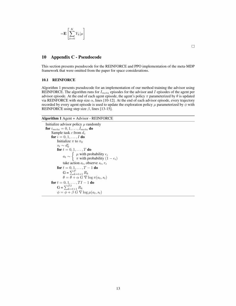
Algorithm 1 presents pseudocode for an implementation of our method training the advisor usingREINFORCE. The algorithm runs for Imeta episodes for the advisor and I episodes of the agent peradvisor episode. At the end of each agent episode, the agent’s policy ⇡ parameterized by ✓ is updatedvia REINFORCE with step size ↵, lines [10-12]. At the end of each advisor episode, every trajectoryrecorded by every agent episode is used to update the exploration policy µ parameterized by � withREINFORCE using step size �, lines [13-15].

Algorithm 1 Agent + Advisor - REINFORCEInitialize advisor policy µ randomlyfor imeta = 0, 1, . . . , Imeta do

Sample task c from dcfor i = 0, 1, . . . , I do

Initialize ⇡ to ⇡0

st ⇠ dc0for t = 0, 1, . . . , T do

at ⇠⇢

µ with probability ✏i⇡ with probability (1� ✏i)

take action at, observe st, rtfor t = 0, 1, . . . , T � 1 do

G =PT

k=t+1 Rk

✓ = ✓ + ↵ G r log ⇡(at, st)

for t = 0, 1, . . . , T I � 1 doG =

PTIk=t+1 Rk

� = �+ � G r logµ(at, st)

13

10.2 Proximal Policy Optimization (PPO)

Pseudocode for a PPO implementation of both agent and advisor is given in Algorithm 2. PPOmaintains two parameterized policies for an agent, ⇡ and ⇡old. The algorithm runs ⇡old for ltime-steps and computes the generalized advantage estimates (GAE), [16], As1 , . . . , Asl , whereAst = �st + (��)�st+1 + · · ·+ (��)l�t+1�sl�1 and �st = rt + �V (st+1)� V (st).

The objective function seeks to maximize the following objective for time-step t:

J = Et

hmin(rtAt, clip(rt, 1� ↵, 1 + ↵)At)

i

� (Rt + � V (st+1)� V (st))2

(4)

where rt = ⇡(at|st)⇡old(at|st) , and V (s) is an estimate of the value for state s. The updates are done in

mini-batches that are stored in a buffer of collected samples.

To train the agent and advisor with PPO we defined two separate sets of policies: µ and µold for theadvisor, and ⇡ and ⇡old for the agent. The agent collects samples of trajectories of length l to updateits policy, while the advisor collects trajectories of length n, where l < n. So, J (the objective ofthe agent) is computed with l samples while Jmeta (the objective of the advisor) is computed with nsamples. In our experiments, setting n � 2l seemed to give the best results.

Notice that the presence of a buffer to store samples, means that the advisor will be storing samplesobtained from many different tasks, which prevents it from over-fitting to one particular problem.

Algorithm 2 Agent + Advisor - PPO1: Initialize advisor policy µ, µold randomly2: for imeta = 0, 1, . . . , Imeta do3: Sample task c from dc4: for i = 0, 1, . . . , I do5: Initialize ⇡ and ⇡old

6: st ⇠ dc07: xt = (st, i, c)8: for t = 0, 1, . . . , T do

9: at ⇠⇢

µold with probability ✏i⇡old with probability (1� ✏i)

10: take action at, observe st, rt11: if t % l = 0 then12: compute As1 , . . . , Asl13: optimize J w.r.t ⇡14: ⇡old = ⇡15: if t % n = 0 then16: compute Ax1 , . . . , Axn

17: optimize Jmeta w.r.t µ18: µold = µ

14

11 Appendix D - Task Variations

This section shows variations of each problem used for experiments.

Pole-balancing: Task variations in this problem class were obtained by changing the mass of thecart, the mass and the length of the pole.

(a) Pole-balancing task 1. (b) Pole-balancing task 2.

Figure 7: Experiments 1 of task variations with discrete action space.

Animat: Task variations in this problem class were obtained by randomly sampling new environments,and changing the start and goal location of the Animat.

(a) Animat task 1. (b) Animat task 2.

Figure 8: Experiments 2 of task variations with discrete action space.

Driving Task: Task variations in this problem class were obtained by changing the mass of the carand turning radius. A decrease in body mass and increase in turning radius causes the car to driftmore and become more unstable when taking sharp turns.

15

(a) Driving task 1. (b) Driving task 2.

Figure 9: Experiments 3 of task variations with discrete action space.

Hopper: Task variations for Hopper consisted in changing the length of the limbs, causing policieslearned for other hopper tasks to behave erratically.

(a) Hopper task 1. (b) Hopper task 2.

Figure 10: Experiments 1 of task variations with continuous action space.

Ant: Tasks variation for Ant consisted in changing the length of the limbs in the ant and the size ofthe body.

(a) Ant task 1. (b) Ant task 2.

Figure 11: Experiments 2 of task variations with continuous action space.

16