ARTICLEdoi:10.1038/nature13186

A mesoscale connectome of themouse brainSeung Wook Oh1*, Julie A. Harris1*, Lydia Ng1*, Brent Winslow1, Nicholas Cain1, Stefan Mihalas1, Quanxin Wang1, Chris Lau1,Leonard Kuan1, Alex M. Henry1, Marty T. Mortrud1, Benjamin Ouellette1, Thuc Nghi Nguyen1, Staci A. Sorensen1,Clifford R. Slaughterbeck1, Wayne Wakeman1, Yang Li1, David Feng1, Anh Ho1, Eric Nicholas1, Karla E. Hirokawa1, Phillip Bohn1,Kevin M. Joines1, Hanchuan Peng1, Michael J. Hawrylycz1, John W. Phillips1, John G. Hohmann1, Paul Wohnoutka1,Charles R. Gerfen2, Christof Koch1, Amy Bernard1, Chinh Dang1, Allan R. Jones1 & Hongkui Zeng1

Comprehensive knowledge of the brain’s wiring diagram is fundamental for understanding how the nervous systemprocesses information at both local and global scales. However, with the singular exception of the C. elegans microscaleconnectome, there are no complete connectivity data sets in other species. Here we report a brain-wide, cellular-level,mesoscale connectome for the mouse. The Allen Mouse Brain Connectivity Atlas uses enhanced green fluorescent protein(EGFP)-expressing adeno-associated viral vectors to trace axonal projections from defined regions and cell types, andhigh-throughput serial two-photon tomography to image the EGFP-labelled axons throughout the brain. This systematicand standardized approach allows spatial registration of individual experiments into a common three dimensional (3D)reference space, resulting in a whole-brain connectivity matrix. A computational model yields insights into connectionalstrength distribution, symmetry and other network properties. Virtual tractography illustrates 3D topography amonginterconnected regions. Cortico-thalamic pathway analysis demonstrates segregation and integration of parallelpathways. The Allen Mouse Brain Connectivity Atlas is a freely available, foundational resource for structural andfunctional investigations into the neural circuits that support behavioural and cognitive processes in health and disease.

A central principle of neuroscience is that the nervous system is a net-work of diverse types of neurons and supporting cells communicatingwith each other mainly through synaptic connections. This overall brainarchitecture is thought to be composed of four systems—motor, sens-ory, behavioural state and cognitive—with parallel, distributed and/orhierarchical sub-networks within each system and similarly complex,integrative interconnections between different systems1. Specific groupsof neurons with diverse anatomical and physiological properties popu-late each node of these sub- and supra-networks, and form extraord-inarily intricate connections with other neurons located near and far.Neuronal connectivity forms the structural foundation underlying neuralfunction, and bridges genotypes and behavioural phenotypes2,3. Connec-tivity patterns also reflect the evolutionary conservation and divergencein brain organization and function across species, as well as both thecommonality among individuals within a given species and the unique-ness of each individual brain.

Despite the fundamental importance of neuronal connectivity, ourknowledge of it remains remarkably incomplete. C. elegans is the onlyspecies for which an essentially complete wiring diagram of its 302 neu-rons has been obtained through electron microscopy4. Histological tracttracing studies in a wide range of animal species has generated a richbody of knowledge that forms the foundation of our current understand-ing of brain architecture, such as the powerful idea of multi-hierarchicalprocessing in sensory cortical systems5. However, much of these dataare qualitative, incomplete, variable, scattered and difficult to retrieve.Thus, our knowledge of whole-brain connectivity is fragmented, with-out a cohesive and comprehensive understanding in any single verte-brate animal species (see for example the BAMS database for the ratbrain6). With recent advances in both computing power and optical imag-ing techniques, it is now feasible to systematically map connectivity

throughout the entire brain. A salient example of this is the ongoingeffort in mapping connections in the Drosophila brain7,8.

The connectome9 refers to a comprehensive description of neuronalconnections, for example, the wiring diagram of the entire brain. Giventhe enormous range of connectivity in the mammalian brain and therelative inaccessibility of the human brain, such descriptions can existat multiple levels: macro-, meso- or microscale. At the macroscale, long-range, region-to-region connections can be inferred from imaging white-matter fibre tracts through diffusion tensor imaging (DTI) in the livingbrain10. However, this is far from cellular-level resolution, given the sizeof single volume elements (voxels .1 mm3). At the microscale, con-nectivity is described at the level of individual synapses, for example,through electron microscopic reconstruction at the nanometer scale4,11–15.At present, the enormous time and resources required for this approachmakes it best suited for relatively small volumes of tissue (,1 mm3). Atthe mesoscale, both long-range and local connections can be describedusing a sampling approach with various neuroanatomical tracers thatenable whole-brain mapping in a reasonable time frame across manyanimals. In addition, cell-type-specific mesoscale projects have the poten-tial to dramatically enhance our understanding of the brain’s organ-ization and function because cell types are fundamental cellular unitsoften conserved across species16,17.

Here we present a mesoscale connectome of the adult mouse brain,The Allen Mouse Brain Connectivity Atlas. Axonal projections fromregions throughout the brain are mapped into a common 3D space usinga standardized platform to generate a comprehensive and quantitativedatabase of inter-areal and cell-type-specific projections. This Connec-tivity Atlas has all the desired features summarized in a mesoscale con-nectome position essay18: brain-wide coverage, validated and versatileexperimental techniques, a single standardized data format, a quantifiable

*These authors contributed equally to this work.

1Allen Institute for Brain Science, Seattle, Washington 98103, USA. 2Laboratory of Systems Neuroscience, National Institute of Mental Health, Bethesda, Maryland 20892, USA.

0 0 M O N T H 2 0 1 4 | V O L 0 | N A T U R E | 1

Macmillan Publishers Limited. All rights reserved©2014

and integrated neuroinformatics resource and an open-access publiconline database.

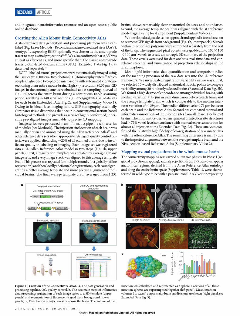
Creating the Allen Mouse Brain Connectivity AtlasA standardized data generation and processing platform was estab-lished (Fig. 1a, see Methods). Recombinant adeno-associated virus (AAV),serotype 1, expressing EGFP optimally was chosen as the anterogradetracer to map axonal projections19,20. We also confirmed that AAV wasat least as efficient as, and more specific than, the classic anterogradetracer biotinylated dextran amine (BDA) (Extended Data Fig. 1), asdescribed separately21.

EGFP-labelled axonal projections were systematically imaged usingthe TissueCyte 1000 serial two-photon (STP) tomography system22, whichcouples high-speed two-photon microscopy with automated vibratomesectioning of an entire mouse brain. High x–y resolution (0.35mm) 2Dimages in the coronal plane were obtained at a z-sampling interval of100-mm across the entire brain during a continuous 18.5 h scanningperiod, resulting in 140 serial sections (a ,750 gigabyte (GB) data set)for each brain (Extended Data Fig. 2a and Supplementary Video 1).Owing to its block-face imaging nature, STP tomography essentiallyeliminates tissue distortions that occur in conventional section-basedhistological methods and provides a series of highly conformed, inher-ently pre-aligned images amenable to precise 3D mapping.

Image series were processed in an informatics pipeline with a seriesof modules (see Methods). The injection site location of each brain wasmanually drawn and annotated using the Allen Reference Atlas23 andother reference data sets when appropriate. Stringent quality control cri-teria were applied, discarding ,25% of all scanned brains due to insuf-ficient quality in labelling or imaging. Each image set was registeredinto a 3D Allen Reference Atlas model in two steps (Fig. 1b, upperpanels). First, a registration template was created by averaging manyimage sets, and every image stack was aligned to this average templatebrain. This process was repeated for multiple rounds, first globally (affineregistration) and then locally (deformable registration), each round gen-erating a better average template and more precise alignment of indi-vidual brains. The final average template brain, averaged from 1,231

brains, shows remarkably clear anatomical features and boundaries.Second, the average template brain was aligned with the 3D referencemodel, again using local alignment (Supplementary Video 2).

We developed a signal detection approach and applied it to each sectionto segment GFP signals from background (Fig. 1b, lower panels). Signalswithin injection site polygons were computed separately from the restof the brain. The segmented pixel counts were gridded into 100 3 1003 100mm3 voxels to create an isotropic 3D summary of the projectiondata. These voxels were used for data analysis, real-time data and cor-relative searches, and visualization of projection relationships in theBrain Explorer.

Meaningful informatics data quantification and comparison relieson the mapping precision of the raw data sets into the 3D referenceframework. We investigated registration variability in two ways. First,we selected 10 widely distributed anatomical fiducial points to comparevariability among 30 randomly selected brains (Extended Data Fig. 2b).We found a high degree of concordance among individual brains, withmedian variation , 49mm in each dimension between each brain andthe average template brain, which is comparable to the median inter-rater variation of , 39mm. The median difference is , 71mm betweeneach brain and the Reference Atlas. Second, we compared manual andinformatics annotations of the injection sites from all Phase I (see below)brains. The informatics-derived assignment of injection site structureshad . 75% voxel-level concordance with manual expert annotation foralmost all injection sites (Extended Data Fig. 2c). These analyses con-firmed the relatively high fidelity of co-registration of raw image datawith the Allen Reference Atlas. The remaining difference is mainly dueto the imperfect alignment between the average template brain and theNissl-section-based Reference Atlas (Supplementary Video 2).

Mapping axonal projections in the whole mouse brainThe connectivity mapping was carried out in two phases. In Phase I (re-gional projection mapping), axonal projections from 295 non-overlappinganatomical regions, defined from the Allen Reference Atlas ontologyand tiling the entire brain space (Supplementary Table 1), were charac-terized in wild-type mice with a pan-neuronal AAV vector expressing

1 mm

a

Stereotaxic injection

Image acquisition

Data QC and injection siteannotation

Informatics processing

Online database

b

c

Single specimen Average template brain 3D reference model

100 μm voxel

Whole brain = 493,878 voxels

1 mm

1 mm

Pre-pipeline activities

EGFP WPRE pApSyn

EGFP

WPRE pApCAG

Cre-independent AAV tracer

Cre-dependent AAV tracer

Isoco

rtexOLFHPF

CTXspSTR

PAL TH HY MB P MY CB All0.0

0.1

0.2

0.3

0.4

0.5

Inje

ctio

n si

te v

olum

e(m

m3 )

Figure 1 | Creation of the Connectivity Atlas. a, The data generation andprocessing pipeline. QC, quality control. b, The two main steps of informaticsdata processing: registration of each image series to a 3D template (upperpanels) and segmentation of fluorescent signal from background (lowerpanels). c, Distribution of injection sites across the brain. The volume of the

injection was calculated and represented as a sphere. Locations of all theseinjection spheres are superimposed together (left panel). Mean injectionvolumes ( 6 s.e.m.) across major brain subdivisions are shown (right panel, seeExtended Data Fig. 3).

RESEARCH ARTICLE

2 | N A T U R E | V O L 0 | 0 0 M O N T H 2 0 1 4

Macmillan Publishers Limited. All rights reserved©2014

EGFP under the human synapsin I promoter (AAV2/1.pSynI.EGFP.WPRE.bGH, Fig. 1a). In Phase II (Cre driver based projection mapping),axonal projections from genetically defined neuronal populations arecharacterized in Cre driver mouse lines with a Cre-dependent AAV(AAV2/1.pCAG.FLEX.EGFP.WPRE.bGH, Fig. 1a). We only report hereon the completed Phase I study, which includes 469 image sets withinjection sites covering nearly the entire brain (Fig. 1c, Extended DataFig. 3 and Supplementary Video 3). Only 18 intended structures werecompletely missed due to redundancy or injection difficulty (Supplemen-tary Table 1).

We examined multiple projection data sets in detail and found thatthey were complete in capturing all known projection target sites through-out the brain, sensitive in detecting thin axon fibres, and consistent inquality to allow qualitative and quantitative comparisons. As an example,7 representative isocortical injections (Fig. 2) reveal distinct projectionpatterns in the striatum, thalamus, zona incerta, midbrain, pons andmedulla. To compare the brain-wide spatial distribution of projectionsbetween cortical source regions, we placed each isocortical injection exper-iment into one of 9 broad functional groups: frontal, motor, anteriorcingulate, somatosensory, auditory, retrosplenial, visual, ventral and asso-ciational areas (Extended Data Fig. 4). The average percentages of totalprojection signals into 12 major brain subdivisions showed dispropor-tionately large projections within the isocortex, as well as distinct sub-cortical distributions.

Brain-wide connectivity matrixAfter segmentation and registration, we derived quantitative values fromsegmented signals in each of the ,500,000 voxels contained within eachbrain. We constructed a brain-wide, inter-areal, weighted connectivitymatrix using the entire Phase I experimental data set (Fig. 3, see Sup-plementary Table 2 for the underlying values). The Allen ReferenceAtlas contains 863 grey-matter structures at the highest level of theontology tree (Supplementary Table 1). We focused our analyses on thechosen 295 structures, which are at a mid-ontology level correspond-ing best with the approximate size of the tracer infection areas (forexample, isocortical areas are not subdivided by layers in this matrix),

but our techniques may be used at deeper levels in future studies. Theprojection signal strength between each source and target was definedas the total volume of segmented pixels in the target (summed acrossall voxels within each target), normalized by the injection site volume(total segmented pixels within the manually drawn injection area).

The majority of the 469 Phase I image sets are single injections intospatially distinct regions, but a subset of these are repeated injectionsinto the same regions. To assess the consistency of projection patternsacross different animals and the reliability of using a single experimentto define connections from any particular region, we compared brain-wide connectivity strengths in 12 sets of duplicate injections (ExtendedData Fig. 5). Each pair was highly correlated across a range of projec-tion strengths. Differences between any two points were on average onlya half order of magnitude (within one standard deviation). In primatecortex, single tracer injections were also found to reliably predict meanvalues obtained from repeated injections into the same source24.

The AAV tracer expresses cytoplasmic EGFP, which labels all pro-cesses of the infected neuron, including axons and synaptic terminals.Signals associated with the major fibre tracts of the brain, marked inthe Allen Reference Atlas, were removed before the informatics quan-tification. However, there are also areas (for example, striatum) whereaxons pass through without making synapses. Although passing fibrescan generally be distinguished from terminal zones by visual inspec-tion of morphology in the 2D images (axons in terminal zones ramifyand contain synaptic boutons, see Extended Data Fig. 6), it is difficultto confidently make this distinction algorithmically. We comparedresults of terminal labelling using Synaptophysin-EGFP-expressing AAVwith the cytoplasmic EGFP AAV (Extended Data Fig. 6). Outside ofmajor fibre tracts, there was high correspondence between synapticEGFP and cytoplasmic EGFP signals in target regions. Nonetheless, itshould be noted that the connectivity matrix contains passing fibresignals within grey matter, the nature of which should be manuallyexamined in 2D section images.

This connectivity matrix (Fig. 3) has several striking features. First,connectivity strengths span a greater than 105-fold range across thebrain (Extended Data Fig. 7), suggesting that quantitative descriptions

MOp

Inje

ctio

n si

teS

tria

tum

Thal

amus

Mid

brai

nM

edul

laP

ons

Zona

ince

rta

Who

le b

rain

ACAd RSPdAUDd VISpORBvl SSp-bfd

VAL

VPM

APN

TRN

IRN

LD

SCm

PG

LD

PPT

TRN

MG

IC

PG

LGd

SCs

PG

MD

SMT

PAG

CS

IO

TRN

SPVI

VPM

APN

2 mm

2 mm

0.5 mm

0.5 mm

0.25 mm

0.5 mm

0.5 mm

0.5 mm

Figure 2 | Whole brain projection patterns fromseven representative cortical regions. Onecoronal section at the centre of each injection site isshown in the top row (see Supplementary Table 1for the full name of each region). In the second row,3D thumbnails of signal density projected onto asagittal view of the brain reveal differences in brain-wide projection patterns. The bottom 6 rows showexamples of EGFP-labelled axons in representativesubcortical regions.

ARTICLE RESEARCH

0 0 M O N T H 2 0 1 4 | V O L 0 | N A T U R E | 3

Macmillan Publishers Limited. All rights reserved©2014

of connectivity must be considered for understanding neural networkproperties24. Second, there are prevalent bilateral projections to cor-responding ipsilateral and contralateral target sites, with ipsilateral pro-jections generally stronger than contralateral ones (total normalizedprojection volumes from all experiments are 4.3:1 between ipsilateraland contralateral hemispheres). Third, of all possible connections, strongconnections are found in only a small fraction. Whereas 63% ipsilateraland 51% contralateral targets have projection strength values above theminimal true positive level of 1024 (which has a potential false positiverate of 27%, Extended Data Fig. 7), only 21% ipsilateral and 9% contra-lateral targets have projection strength values above the intermediatelevel of 1022.

An inter-region connectivity modelInfected neurons in injection sites often span several brain areas. Tobetter describe the mutual connection strengths between ontologicallydefined regions rather than injection sites, we constructed inter-regionconnectivity matrices via a computational model (see SupplementaryNotes for a detailed description), using segmented projection volumes(Fig. 3) to define connection strengths. Two basic modelling assump-tions were used. The first, regional homogeneity, assumes that projectionsbetween source X and target Y regions are homogeneously distributed,so that infection of a subarea of the region is representative of the entireregion. This allows the value of WX,Y , a regional connectivity measure,to be inferred from data that can at best only sample the source region.The second assumption, projection additivity, assumes that the projec-tion density of multiple source regions sum linearly to produce projec-tion density in a target region. This allows relative contributions of differentsources to be determined for a target region, assuming at least partiallyindependent injections.

The 469 experiments allowed us to compute the mutual connectionsamong 213 regions. The best-fit model (Fig. 4a, see SupplementaryTable 3 for the underlying values) results from a bounded optimizationfollowed by a linear regression to determine connection coefficients,assigning statistical confidence (P values) to each connection in thematrix. Based on the bounded optimization, the number of non-zeroentries provides an upper bound estimate for sparsity: 36% for theentire brain and 52% for cortico-cortical connections. Using confid-ence values for each non-zero connection, the lower bound on sparsityis 13% for the entire brain and 32% for cortico-cortical connections.

Connection strengths spanned ,105-fold range, and negatively cor-related with the distance between connected regions (SupplementaryNotes and Supplementary Table 4). Based on the Akaike informationcriterion (AIC), among hypothesized connection strength distributions(lognormal, normal, exponential, inverse Gaussian) the brain-wide dataare best fit by a lognormal distribution (Fig. 4b, red lines). However, thelog-transformed connection strengths failed to pass the Shapiro-Wilktest for normality (ipsilateral: P 5 0.039; contralateral: P 5 0.023), andamong Gaussian mixture models, a two-component one provided thebest fit (Fig. 4b, green lines). For cortico-cortical connections, both intra-and inter-hemispheric distributions are well fit by lognormals (ipsilateral:P 5 0.23; contralateral: P 5 0.21) individually (Fig. 4b), but they aredifferent enough that when combined the distribution is no longer lognor-mal (P 5 0.0019). This extends previously reported findings that cortico-cortical connections follow a lognormal distribution in the primate24,25

and mouse cortex26 to the entire mouse brain. These observations com-bined indicate that connections might be lognormally distributed withina region, yet vary systematically with statistics unique to the region.

Previous studies on connectivity considered global organizationalprinciples from a graph-theory perspective26–28. We transformed our

Target: right hemisphere (ipsilateral) Target: left hemisphere (contralateral)

Iso-cortex O

LFH

PF

CTX

spS

TR PAL Thal Hypo-

thalMid-brain P

ons

Medulla CB

Iso-cortex

OLF

HPF

CTXsp

STR

PAL

Thal

Hypo-thal

Mid-brain

Pons

Medulla

CB

Sou

rce

(inje

ctio

ns)

Log10

–3.5 –2.0 –0.5

Iso-cortex O

LF

HP

FC

TXsp

STR PA

L Thal Hypo-thal

Mid-brain P

ons

Medulla CB

Figure 3 | Adult mouse brain connectivity matrix. Each row shows thequantitative projection signals from one of the 469 injected brains to each of the295 non-overlapping target regions (in columns) in the right (ipsilateral) andleft (contralateral) hemispheres. Both source and target regions are displayed inontological order. The colour map indicates log10-transformed projection

strength (raw values in Supplementary Table 2). All values less than 1023.5 areshown as blue to minimize false positives due to minor tissue and segmentationartefacts and all values greater than 1020.5 are shown as red to reduce thedominant effect of projection signals in certain disproportionately large regions(for example, striatum).

RESEARCH ARTICLE

4 | N A T U R E | V O L 0 | 0 0 M O N T H 2 0 1 4

Macmillan Publishers Limited. All rights reserved©2014

weighted, directed, connectivity matrix (Fig. 4a) to binary directed andbinary undirected data sets. Network analyses (Fig. 4c, see also Sup-plementary Notes) reveal that the mouse brain has a higher meanclustering coefficient (which gives the ratio of existing over possibleconnections), 0.42, than expected by a random network29,30 with identicalsparseness, 0.12. Random graphs with matched node degree distributionshow a similar drop in clustering coefficient to 0.16. A ‘small-world’network model31 approximates the clustering coefficient distributionafter being fit to its mean; however, its node degree distribution poorlymatches the data. Here, a better fit is achieved with a scale-free net-work32; however, neither model simultaneously fits both distributions.

Next, we analysed similarity in connection patterns between differ-ent regions. Similarity is characterized by two measures: correlationsbetween outgoing projections originating in two areas and correlationsbetween incoming projections ending in these two areas. Figure 4d depictsheat maps of correlation coefficients between the same regions of thelinear model (Fig. 4a) depicted across the rows (that is, as a commonsource for other regions), and down the columns (that is, as a commontarget from other regions). The number of strong correlations is largerthan expected by chance, suggesting a tendency of regions to organizeinto clusters to allow for strong indirect connectivity.

The cortico-striatal-thalamic networkDifferent cortical areas project to different domains of striatum andthalamus with some degree of topography33–35. We used 80 isocorticalinjection experiments to examine this. Spearman’s rank correlationcoefficient of segmented projection volumes of all voxels across the entirebrain was computed between every pair of experiments, and hierarch-ical clustering led to 21 distinct groups, each containing 1 to 10 injections

(Extended Data Fig. 8a, b). Such grouping effectively divides the cortexinto 21 predominantly non-overlapping spatial zones as shown in aflat-map cortex representation (Fig. 5a) defined by similar output pro-jections. To effectively visualize different projection patterns in a com-mon 3D space, voxel densities from 21 selected injections, one (centrallylocated) from each cluster, were overlaid to create ‘dotograms’ (Fig. 5b,c and Extended Data Fig. 8c), demonstrating that projections fromdifferent cortical regions divide up striatum and thalamus into distinctdomains.

Average inter-group distances (Extended Data Fig. 9a–d) were usedto quantify the degree to which inter-group spatial relationships withinthe cortex are preserved in target domains. Distance matrices for bothipsilateral and contralateral cortical targets were highly correlated withthe distance matrix of injection sites, as were ipsilateral striatal and tha-lamic distance matrices. Weaker correlations were observed in contra-lateral striatum and thalamus. The computed distance matrices showthat the spatial relationship between injection sites is recapitulated inthe projections to striatum and thalamus, with some transformation ofscale and rotation.

This highly synchronized topography can be determined via virtualtractography. Real tractography (following single axons) cannot be donebecause of the discrete 100-mm sampling between sections. Instead, fromevery voxel we computed a path back to the injection site by finding theshortest density-weighted distance through the voxels. The 3D tracto-graphy paths were plotted for both cortical hemispheres (Fig. 5d andExtended Data Fig. 9e), ipsilateral striatum and thalamus (Fig. 5e, f).The tractography shows that the paths themselves also retain the samespatial organization. In particular for the thalamus, anterior groups passthrough fibre tracts in the striatum, narrowing through the globus pallidus,

Node degree

Connection strength

ProbabilityC

ount

Clustering coefficient

PD

F

Reg

ion

X

Region Y Region Y

0.75

0.60

0.45

0.30

0.15

0.00

–0.15

–0.30

0.90

Contra

Who

le b

rain

Cor

tico-

cort

ical

Target (ipsi)

MY

PMB

HY

THPAL

STR

CTX

spH

PF

OLF

Isoc

orte

x

CB

MY

MB

HY

TH

PALSTR

CTXspHPFOLF

Isocortex

CB

MY

PMB

HY

THPAL

STR

CTX

spH

PF

OLF

Isoc

orte

x

CB

Target (contra)S

ourc

e

Connection strength

P value

101

100

10–1

10–2

10–3

dc

ba

Contra

Ipsi

Ipsi

0.4

0.2

0.6

0.20.2

0.1

040200 60 0.75

Watts-Strogatz

Barabasi-Albert

Erdos-Renyl

Shuffled

0.50.250 1

0.3

0.2

0.4

0.1

0

0.0

100

50

150

0

80

40

120

0

4020

60

0

30

15

10010–110–210–3 101

45

0

0.4

0.2

0.6

0.0

0.40.2

0.60.8

0.0

0.40.2

0.60.8

0.0

Sourcecorrelation:

XY

Targetcorrelation:

XY

1 0.5 0

Figure 4 | A computational model of inter-regional connection strengths.a, The inter-region connectivity matrix, with connection strengths representedin colours and statistical confidence depicted as an overlaid opacity. Notethat in this matrix, the sources (rows) are regions, whereas for the matrix ofFig. 3, the sources are injection sites. b, Both whole-brain and cortico-corticalconnections can be fit by one-component lognormal distributions (red lines).However, the log distributions of whole-brain connection strengths are best

fit by a two-component Gaussian mixture model (green lines). c, Nodedegree and clustering coefficient distributions for a binarized version of thelinear model network, compared against Erdos-Renyi, Watts-Strogatz andBarabasi-Albert networks with matched graph statistics. d, Comparison ofthe correlation coefficients of normalized connection density between areas,defined as the common source for projections to other regions (left) and asthe common target of projections from other regions (right).

ARTICLE RESEARCH

0 0 M O N T H 2 0 1 4 | V O L 0 | N A T U R E | 5

Macmillan Publishers Limited. All rights reserved©2014

before spreading throughout the thalamus (Extended Data Fig. 9f). Pos-terior groups (RSP, VIS) bypass the striatum but retain a strict topo-graphy following the medial/lateral axis (Fig. 5f).

Although the striatum is a cellularly homogeneous structure thatcan be subdivided into distinct domains selectively targeted by corticaland other inputs36 (Fig. 5e), the thalamus is highly heterogeneous, com-posed of up to 50 discrete nuclei37, receiving and relaying diverse sensory,motor, behavioural state and cognitive information in parallel pathwaysto and from the isocortex. We constructed a comprehensive wiring dia-gram between major, functionally distinct cortical regions and thalamicnuclei in the ipsilateral hemisphere (Fig. 6 and Extended Data Fig. 10),by combining the quantitative connectivity matrix (Fig. 3) with the linearmodel (Fig. 4a), manual proof-checking in the raw image sets, and cross-referencing published literature (83 publications, mostly from rat data,see Extended Data Fig. 10). This wiring diagram demonstrates specificpoint-to-point interconnections between corresponding clusters thatdivide the cortico-thalamic system into six functional pathways: visual,somatosensory, auditory, motor, limbic and prefrontal. We also observedcross-talk between these pathways, mediated by specific associationalcortical areas and integrative thalamic nuclei.

The specific observations from our data are mostly consistent (witha few additions) with extensive previous studies in rats and the fewernumber of studies in mice (Extended Data Fig. 10) as well as with studiesin other mammalian species37–39, providing a comprehensive and uni-fying view of mouse cortico-thalamic connections for the first time.Much work is still needed to obtain a full picture of connectivity in thecortico-thalamic system, including intra-cortical and intra-thalamic con-nections, their relationships with the interconnections between cortex

and thalamus, and the exquisite cortical laminar specificity of the ori-ginating and terminating zones of many of these connections5,38,40.

DiscussionThe standardized projection data set and the informatics frameworkbuilt around it provide a brain-wide, detailed and quantitative connec-tivity map that is the most comprehensive, to date, in any vertebratespecies. The high-throughput whole-brain mapping approach is remark-ably consistent across animals, with an average correlation of 0.90 across12 duplicate sets of mice (Extended Data Fig. 5). Informatics proces-sing of the data set, such as co-registration and voxelization, helps withdirect comparison between any image series, and systematic modellingand computational analyses of the entire network. Furthermore, theentire data set preserves the 3D spatial relationship of different domains,pathways and topography (Fig. 5). Thus, our connectivity atlas lays thegroundwork for large-scale analyses of global neural networks, as wellas networks within and between different neural systems.

As an initial analysis of this large-scale data set, we present an exam-ination of both general principles of whole brain architecture and spe-cific properties of cortical connections. We found that projections withinthe ipsilateral hemisphere and to the corresponding locations in the con-tralateral hemisphere are remarkably similar across the brain (Figs 3and 4; Pearson’s r 5 0.595), with the contralateral connection strengthssignificantly weaker than ipsilateral ones. The mouse brain shows defin-ing features of both small-world and scale-free networks, that is, itclusters and has hubs; but neither of these models in isolation can fullyexplain it. Interestingly, the connection strengths at both cortico-corticaland whole-brain levels show lognormal distributions, that is, long-tailed

GU

AI

AId

SSs

ORBvl

SSs

ORBm

SSs

SSsORBl

AUDv

SSp−m

PL

SSs

SSp−un

MOp

ACAv

SSp−m

SSp−mMOp

AUDd

VISl

AUDd

AUDd

SSp−ul

SSp−bfd

SSp−bfd

AUDd

SSp−bfd

VISp

MOs

SSp−bfd

SSp−bfd

MOs

MOp

ACAd

VISal

SSp−ll

MOp

SSp−trSSp−tr

SSp−tr

MOs

SSp−ll

SSp−ll

VISp

VISp

RSPv

PTLpRSP

PTLp

SSp−ll

RSPagl

VISam

VISp

MOp

AIdORBvlORBm

ORBl

AUDv

AId

PL

AId

MOp

ACAv

MOsMOp

MOp

AUDd

ACAd

VISlVISl

TEa

AUDdAUDd

SSp−ul

VISp

SSp−bfd

SSp−bfd

SSp−bfd

MOs

VISp

SSp−bfd

SSp−bfdACAvMOs

ACAd

MOp

SSp−bfdACAdSSp−ll

MOpSSp−tr

MOpSSp−trSSp−tr

MOs SSp−llSSp−tr

SSp−ll

VISpRSP RSPvPTLp

SSp−llPTLpVISam

MOp

a

Bregma:0.25 mm –0.25 mm –0.75 mm –1.25 mm –1.75 mm –2.25 mm –2.75 mm –3.25 mm

CPTH

c

b

Isocortex Caudoputamen Thalamusd e f

1 mm

A P

M

LMOp

MOp

MOp

MOp

MOp

MOpMOp

MOp

MOp

MOs

MOsMOs

MOs

MOs

MOs

SSp−bfd

SSp−bfd

SSp−bfdSSp−bfd

SSp−bfdSSp−bfd

SSp−ll

SSp−llSSp−ll

SSp−ll

SSp−mSSp−m

SSp−m

SSp−ul

SSp−tr

SSp−tr

SSp−tr

SSp−tr

SSp−un

SSs SSs

SSs SSsSSs

SSs

GU

AUDdAUDd

AUDd AUDdAUDd AUDd

AUDv

VISal

VISam

VISlVISl

VISpVISp

VISp

VISp

VISp

VISp

VISp

ACAd

ACAdACAd

ACAv

ACAv

PL

ORBl

ORBm

ORBvlORBvl

AI

AIdAId

AId

RSP

RSPagl

RSPagl

RSPv

PTLpPTLp

TEa

Figure 5 | Topography of cortico-striatal and cortico-thalamicprojections. a, Cortical domains inthe cortex flat-map. Each circlerepresents one of 80 cortical injectionexperiments, whose location isobtained via multidimensionalscaling from 3D to allowvisualization of all the sites in one 2Dplane. The size of the circle isproportional to the injection volume.Clustered groups from ExtendedData Fig. 8b are systematicallycolour-coded. The selected injectionsfor b are marked with a black outline.b, For co-visualization, voxeldensities from the 21 selectedinjections from a are overlaid as‘dotograms’ at 8 coronal levels foripsilateral hemisphere. For thedotogram, one circle, whose size isproportional to the projectionstrength, is drawn for each injectionin each voxel; the circles are sorted sothat the largest is at the back and thesmallest at the front, and are partiallyoffset as a spiral. c, Enlarged viewof the dotogram from the areaoutlined by a white box in b. d, 3Dtractography paths in both corticalhemispheres. e, A medial view of3D tractography paths into theipsilateral caudoputamen. Voxelstarting points are represented asfilled circles and injection site endpoints as open circles. f, A top-downview of 3D tractography paths intothe ipsilateral thalamus.

RESEARCH ARTICLE

6 | N A T U R E | V O L 0 | 0 0 M O N T H 2 0 1 4

Macmillan Publishers Limited. All rights reserved©2014

distributions with small numbers of strong connections and large num-bers of weak connections. In connections among isocortex, striatum andthalamus, clustering analysis and virtual tractography recapitulate ana-tomical parcellation and topography of functional domains and pro-jection pathways (Fig. 5). The extensive reciprocal connections betweenisocortex and thalamus (Fig. 6) further illustrate general principles ofnetwork segregation and integration.

Our Connectivity Atlas represents a first systematic step towardsthe full understanding of the complex connectivity in the mammalianbrain. Through the process, limitations of the current approach andopportunities for future improvement can be identified. On the tech-nical side, any potential new connections identified in the Phase I dataset (which does not yet have extensive redundancy in regional coverage)will need to be confirmed with more data. Also, we cannot exclude thepossibility that the AAV tracer we chose to use (with the specific pro-moter and serotype) may not be completely unbiased in labelling all neur-onal types. The connectivity matrix has been shown to contain falsepositive signals (Extended Data Fig. 7), mainly due to tissue and imag-ing artefacts and injection tract contaminations. The connectivity matrixbased on cytoplasmic EGFP labelling does not distinguish passing fibresfrom terminal zones, and examination of raw images is needed to helpwith such distinction, using features such as ramification of axon fibres,and boutons or enlargements in axons. The Atlas could also be enhancedin the future with more systematic mapping using synaptic-terminal-specific viral tracers as shown (Extended Data Fig. 6). Regarding signalquantification, we chose to use projection volume (sum of segmentedpixel counts) over projection fluorescence intensity (sum of segmentedpixel intensity), because we found the former more reliable and lessvariable across different brains (even after normalization). However,the use of projection volume will probably underestimate the strengthof dense projections. Thus, the true range of projection strengths maygo beyond the 105-fold reported here. Finally, we observed that thealignment between the average template brain and our existing ReferenceAtlas model (which was drawn upon Nissl sections) is not perfect, which

leads to a degree of registration imprecision that could affect the accu-racy of the quantitative connectivity matrices. Our work shows the needto generate a new reference model based on a realistic 3D brain, such asthe average template brain presented here. Our data set can also helpthis by adding connectivity information to improve anatomical deli-neations previously defined solely by cyto- and chemoarchitecture.

Beyond the above technical issues, identities of the postsynaptic neu-rons at the receiving end of the mapped connections are not labelledand therefore unknown. Microscale, synaptic-level details are missing,and electrical connections through gap junctions are not revealed. More-over, our mesoscale connectome provides a static, structural connecti-vity map, which is necessary but insufficient for understanding function.Moving from here to functional connectivity and circuit dynamics ina living brain will require fundamentally different approaches41. Oneimportant aspect concerns the types of synapses present in each conne-ctional path, as determined by their neurotransmitter contents and theirphysiological properties. Anatomical connection strength (for example,numbers of axon fibres and boutons) needs to be combined with phy-siological connection properties (for example, excitatory vs inhibitorytypes of synapses, fast vs slow neurotransmission, and the specific strengthand plasticity of each synapse) to yield a true functional connection strength.

With the goal of bridging structural connectivity and circuit func-tion41, we have taken a genetic approach, using AAV viral tracers thatexpress EGFP in either a pan-neuronal or cell-type-specific manner.The same neural networks mapped here can be further investigated bysimilar viral vectors expressing tools for activity monitoring (for example,genetically encoded calcium indicators) and activity manipulation (forexample, channelrhodopsins)16. Furthermore, our ongoing efforts of Cre-driver dependent tracing will allow more specific connectivity mappingfrom discrete areas and specific functional cell types. Such cell-type-specific connectivity mapping is perhaps the greatest advantage of thegenetic tracing approach, allowing dissection of differential projectionpatterns from different neuronal types that are often intermingled inthe same region. The genetic tracing approach can be further extended

RT

* *

* *

RT

Cortex

Cortex

Thalamus

Thalamus

Figure 6 | A wiring diagram ofconnections between major corticalregions and thalamic nuclei. Upperand lower panels show projectionsfrom cortex to thalamus or fromthalamus to cortex, respectively(ipsilateral projections only). Colourcoding of different cortical regionsand their corresponding thalamicnuclei is similar to the flat-mapcortex in Fig. 5a. Thickness of thearrows indicates projection strength,which is shown in three levels asin Extended Data Fig. 10 andcorresponds roughly to the red,orange and yellow colours in the rawconnectivity matrix (Fig. 3). LGvand PF do not have significantprojections to cortex. The reticularnucleus of the thalamus (RT) (thedashed box) is placed in betweencortex and thalamus to illustrate itsspecial role as a relay nucleus whichall cortico-thalamic and thalamo-cortical projections pass through andmake collateral projections into.The asterisks indicate that cortico-thalamic and thalamo-corticalprojections in the gustatory/visceralpathway are between GU/VISCcortical areas and VPMpc/VPLpcnuclei (instead of VPM/VPL). SeeSupplementary Table 1 for the fullname of each region.

ARTICLE RESEARCH

0 0 M O N T H 2 0 1 4 | V O L 0 | N A T U R E | 7

Macmillan Publishers Limited. All rights reserved©2014

into identification of inter-connected pre- and postsynaptic cell typesand individual cells, using approaches such as retrograde or antero-grade trans-synaptic tracing42–44. Our approach can also be appliedto animal models of human brain diseases and the connectivity datagenerated here can be instructive to human connectome studies, whichwill help to further our understanding of human brain connectivityand its involvement in brain disorders.

METHODS SUMMARYC57BL/6J male mice at age P56 were injected with EGFP-expressing AAV usingiontophoresis by the stereotaxic method. The brains were scanned using the STPtomography systems. Images were subject to data quality control and all the injec-tion sites were manually annotated. All the image sets were co-registered into the3D reference space. EGFP-positive signals were segmented from background, andbinned at voxel levels for quantitative analyses. The raw connectivity data are servedwith various navigation tools on the web through the Allen Institute’s data portal.See the full Methods section for detailed descriptions.

Online Content Any additional Methods, Extended Data display items and SourceData are available in the online version of the paper; references unique to thesesections appear only in the online paper.

Received 22 July 2013; accepted 27 February 2014.Published online 2 April 2014.

1. Swanson, L. W. Brain Architecture: Understanding the Basic Plan 331 (Oxford Univ.Press, 2012).

2. Seung, S. Connectome: How The Brain’s Wiring Makes Us Who We Are 359(Houghton Mifflin Harcourt, 2012).

3. Sporns, O. Networks of the Brain 412 (The MIT Press, 2011).4. White, J. G., Southgate, E., Thomson, J. N. & Brenner, S. The structure of the

nervous system of the nematode Caenorhabditis elegans. Phil. Trans.R. Soc. Lond. B314, 1–340 (1986).

5. Felleman, D. J. & Van Essen, D. C. Distributed hierarchical processing in theprimate cerebral cortex. Cereb. Cortex 1, 1–47 (1991).

6. Bota, M., Dong, H. W. & Swanson, L. W. Combining collation and annotation effortstoward completion of the rat and mouse connectomes in BAMS. Front.Neuroinform. 6, 2 (2012).

7. Chiang, A. S. et al. Three-dimensional reconstruction of brain-wide wiringnetworks in Drosophila at single-cell resolution. Curr. Biol. 21, 1–11 (2011).

8. Jenett, A. et al.A GAL4-driver line resource for Drosophila neurobiology. Cell Rep. 2,991–1001 (2012).

9. Sporns, O., Tononi, G. & Kotter, R. The human connectome: A structuraldescription of the human brain. PLoS Comput. Biol. 1, e42 (2005).

10. Van Essen, D. C. et al. The WU-Minn Human Connectome Project: an overview.NeuroImage 80, 62–79 (2013).

11. Bock, D.D.et al. Networkanatomy and in vivophysiologyof visual cortical neurons.Nature 471, 177–182 (2011).

12. Briggman, K. L., Helmstaedter, M. & Denk, W. Wiring specificity in the direction-selectivity circuit of the retina. Nature 471, 183–188 (2011).

13. Chklovskii, D. B., Vitaladevuni, S. & Scheffer, L. K. Semi-automated reconstructionof neural circuits using electron microscopy. Curr. Opin. Neurobiol. 20, 667–675(2010).

14. Helmstaedter, M. et al. Connectomic reconstruction of the inner plexiform layer inthe mouse retina. Nature 500, 168–174 (2013).

15. Takemura, S. Y. et al. A visual motion detection circuit suggested by Drosophilaconnectomics. Nature 500, 175–181 (2013).

16. Huang, Z. J. & Zeng, H. Genetic approaches to neural circuits in the mouse. Annu.Rev. Neurosci. 36, 183–215 (2013).

17. Masland, R. H. The neuronal organization of the retina. Neuron 76, 266–280(2012).

18. Bohland, J. W. et al. A proposal for a coordinated effort for the determination ofbrainwide neuroanatomical connectivity in model organisms at a mesoscopicscale. PLoS Comput. Biol. 5, e1000334 (2009).

19. Chamberlin, N. L., Du, B., de Lacalle, S. & Saper, C. B. Recombinant adeno-associated virus vector: use for transgene expression and anterograde tracttracing in the CNS. Brain Res. 793, 169–175 (1998).

20. Harris, J. A., Oh, S. W. & Zeng, H. Adeno-associated viral vectors for anterogradeaxonal tracing with fluorescent proteins in nontransgenic and Cre driver mice.Curr. Protoc. Neurosci. 59, 1.20.1–1.20. 18 http://dx.doi.org/10.1002/0471142301.ns0120s59 (2012).

21. Wang, Q. et al. Systematic comparison of adeno-associated virus and biotinylateddextran amine reveals equivalent sensitivity between tracers and novel projectiontargets in the mouse brain. J. Comp. Neurol. http://dx.doi.org/10.1002/cne.23567 (Feb 22, 2014).

22. Ragan, T. et al. Serial two-photon tomography for automated ex vivo mouse brainimaging. Nature Methods 9, 255–258 (2012).

23. Dong, H. W. The Allen Reference Atlas: a Digital Color Brain Atlas of the C57BL/6JMale Mouse (John Wiley & Sons, 2008).

24. Markov, N. T. et al. A weighted and directed interareal connectivity matrix formacaque cerebral cortex. Cereb. Cortex 24, 17–36 (2014).

25. Ercsey-Ravasz, M. et al. A predictive network model of cerebral corticalconnectivity based on a distance rule. Neuron 80, 184–197 (2013).

26. Wang, Q., Sporns, O. & Burkhalter, A. Network analysis of corticocorticalconnections reveals ventral anddorsalprocessingstreams inmouse visual cortex.J. Neurosci. 32, 4386–4399 (2012).

27. Bullmore, E. & Sporns, O. Complex brain networks: graph theoretical analysis ofstructural and functional systems. Nature Rev. Neurosci. 10, 186–198 (2009).

28. Schmitt, O. et al. The intrinsic connectome of the rat amygdala. Front. NeuralCircuits 6, 81 (2012).

29. Erdos, P. & Renyi, A. On the evolution of random graphs. Publ. Math. Inst. Hung.Acad. Sci. 5, 17–61 (1960).

30. Bollobas, B. Random Graphs (Cambridge Univ. Press, 2001).31. Watts, D. J. & Strogatz, S. H. Collective dynamics of ‘small-world’ networks. Nature

393, 440–442 (1998).32. Barabasi, A. L. & Albert, R. Emergence of scaling in randomnetworks.Science 286,

509–512 (1999).33. Groenewegen, H. J. & Berendse, H. W. The specificity of the ‘nonspecific’ midline

and intralaminar thalamic nuclei. Trends Neurosci. 17, 52–57 (1994).34. Joel, D. & Weiner, I. The organization of the basal ganglia-thalamocortical circuits:

open interconnected rather than closed segregated. Neuroscience 63, 363–379(1994).

35. Mailly, P., Aliane, V., Groenewegen, H. J., Haber, S. N. & Deniau, J. M. The ratprefrontostriatal system analyzed in 3D: evidence for multiple interactingfunctional units. J. Neurosci. 33, 5718–5727 (2013).

36. Gerfen, C. R. in The Rat Nervous System (ed. Paxinos, G.) 455–508 (ElsevierAcademic Press, 2004).

37. Jones, E. G. The Thalamus (Cambridge Univ. Press, 2007).38. Jones, E. G. Viewpoint: the core and matrix of thalamic organization. Neuroscience

85, 331–345 (1998).39. Scannell, J. W., Burns, G. A., Hilgetag, C. C., O’Neil, M. A. & Young, M. P. The

connectional organization of the cortico-thalamic system of the cat. Cereb. Cortex9, 277–299 (1999).

40. Barbas, H. & Rempel-Clower, N. Cortical structure predicts the pattern ofcorticocortical connections. Cereb. Cortex 7, 635–646 (1997).

41. Bargmann, C. I. & Marder, E. From the connectome to brain function. NatureMethods 10, 483–490 (2013).

42. Lo, L. & Anderson, D. J. A. Cre-dependent, anterograde transsynaptic viral tracerfor mapping output pathways of genetically marked neurons. Neuron 72,938–950 (2011).

43. Wall, N. R., Wickersham, I. R., Cetin, A., De La Parra, M. & Callaway, E. M.Monosynaptic circuit tracing in vivo through Cre-dependent targeting andcomplementation of modified rabies virus. Proc. Natl Acad. Sci. USA 107,21848–21853 (2010).

44. Wickersham, I. R. et al. Monosynaptic restriction of transsynaptic tracing fromsingle, genetically targeted neurons. Neuron 53, 639–647 (2007).

Supplementary Information is available in the online version of the paper.

Acknowledgements We wish to thank the Allen Mouse Brain Connectivity AtlasAdvisory Councilmembers,D. Anderson, E. M.Callaway,K. Svoboda, J. L. R. Rubenstein,C. B. Saper and M. P. Stryker for their insightful advice. We thank T. Ragan for providinginvaluable support andadvice in the development andcustomizationof the TissueCyte1000 systems. We are grateful for the technical support of the many staff members intheAllen Institutewho are notpart of theauthorship of thispaper. Thisworkwas fundedby the Allen Institute for Brain Science. The authors wish to thank the Allen Institutefounders, P. G. Allen and J. Allen, for their vision, encouragement and support.

Author Contributions H.Z., S.W.O., J.A.H. and L.N. contributed significantly to overallproject design. S.W.O. and H.Z. did initial proof-of-principle studies. J.A.H., M.T.M., B.O.,P.B., T.N.N., K.E.H. and S.A.S. conducted tracer injections and histological processing.B.W., C.R.S., E.N., A.H., P.W. and A.B. carried out imaging system establishment,maintenance, and imaging activities. L.N., C.L., L.K., W.W., Y.L., D.F. and H.P. conductedinformatics data processing and online database development. A.M.H., K.M.J. and Q.W.conducted image quality control and data annotation. N.C., S.M. and C.K. performedcomputational modelling. H.Z., S.W.O., A.R.J., C.D., C.K., A.B., J.G.H., J.W.P. and M.J.H.performed managerial roles. H.Z., J.A.H., L.N., S.M., N.C., Q.W., S.W.O., C.R.G. and C.K.were main contributors to data analysis and manuscript writing, with input from otherco-authors.

Author Information The Allen Mouse Brain Connectivity Atlas is accessible at (http://connectivity.brain-map.org). All AAV viral tracers are available at Penn Vector Core, andAAV viral vector DNA constructs have been deposited at the plasmid repositoryAddgene. Reprints and permissions information is available at www.nature.com/reprints. The authors declare no competing financial interests. Readers are welcome tocomment on the online version of the paper. Correspondence and requests formaterials should be addressed to H.Z. (hongkuiz@alleninstitute.org).

RESEARCH ARTICLE

8 | N A T U R E | V O L 0 | 0 0 M O N T H 2 0 1 4

Macmillan Publishers Limited. All rights reserved©2014

METHODSAll experimental procedures related to the use of mice were approved by theInstitutional Animal Care and Use Committee of the Allen Institute for BrainScience, in accordance with NIH guidelines.Outline of the Connectivity Atlas data generation and processing pipeline. Astandardized data generation and processing platform was established (Fig. 1a).Viral tracers were validated and experimental conditions were established throughpre-pipeline activities. C57BL/6J mice at age P56 were injected with viral tracersusing iontophoresis by the stereotaxic method. Six STP tomography systems gen-erated high-resolution images from up to 6 brains per day. Images were subject todata quality control and all the injection sites annotated. A stack of qualified 2Dimages then underwent a series of informatics processes. The image data and infor-matics products as well as all metadata are stored, retrieved and maintained usingour laboratory information management system (LIMS). The generated connec-tivity data are served with various navigation tools on the web through the AllenInstitute’s data portal along with other supporting data sets.Stereotaxic injections of AAV using iontophoresis. Recombinant adeno-associatedvirus (AAV) expressing EGFP was chosen as the anterograde tracer to map axonalprojections because of several advantages over conventional neuroanatomical tracers19.First, AAV mediates robust fluorescent labelling of the soma and processes of infectedneurons, which can be coupled with direct imaging methods for high-throughputproduction without additional histochemical staining steps. Second, compared toconventional tracers which often have mixed anterograde and retrograde trans-port, retrograde labelling with AAV (except for certain serotypes) is generally negligible.In this study, retrogradely infected cells were seen only rarely. Notable exceptionsare found in specific circuits that might have certain types of strong presynapticinputs, such as the entorhinal cortex projection to hippocampal subregions dentategyrus and CA1, where retrogradely infected input cells can be brightly labelled.Finally, perhaps the greatest advantage of using AAV over conventional tracers isthe flexible molecular strategies that can be used to introduce various transgenesand to label specific neuronal populations by combining cell-type-selective Credriver mice with AAV vectors harbouring a Cre-dependent expression cassette.

To optimize the tracing approach for the large-scale atlas data generation, wetested various AAV constructs, serotypes and injection methods. We selectedAAV vectors that express EGFP at the highest levels. We found that AAV serotype1 produces the most robust and uniform neuronal tropism and that iontophoreticdelivery of AAV gives rise to the most consistent and confined viral infection volume.Thus, the entire atlas data generation was standardized with the use of AAVserotype 1 and iontophoresis for stereotaxic injections20.

Stereotaxic coordinates were chosen for each target area based on The MouseBrain in Stereotaxic Coordinates45. For the majority of target sites, the anterior/posterior (AP) coordinates are referenced from Bregma, the medial/lateral (ML)coordinates are distance from midline at Bregma, and the dorsal/ventral (DV)coordinates are measured from the pial surface of the brain. For several of themost caudal medullary nuclei (for example, gracile nucleus and spinal nucleus ofthe trigeminal, caudal part), the calamus (at the floor of the fourth ventricle) isused as a registration point instead of Bregma. For many cortical areas, injectionswere made at two depths to label neurons throughout all six cortical layers and/orat an angle to infect neurons along the same cortical column. For laterally locatedcortical areas (for example, orbital area, medial part; prelimbic area; agranular insulararea), the injections were made at two adjacent ML coordinates for the same reason,since the pipette angle required for injection along the cortical column is nearly90u, beyond our technical limit. The stereotaxic coordinates used for generatingdata are listed under the Documentation tab in the data portal.

Adult male C57BL/6J mice (stock no. 00064, The Jackson Laboratory, Bar Harbour,ME) were used for AAV tracer (AAV2/1.pSynI.EGFP.WPRE.bGH, Penn VectorCore, Philadelphia, PA) injections at P56 6 2 postnatal days. Mice were anaesthe-tized with 5% isoflurane and placed into a stereotaxic frame (model no. 1900, DavidKopf Instruments, Tujunga, CA). For all injections using Bregma as a registrationpoint, an incision was made to expose the skull and Bregma and Lambda land-marks were visualized using a stereomicroscope. A hole overlying the targeted areawas made by first thinning the skull using a fine drill burr until only a thin layer ofbone remained. A microprobe and fine forceps were used to peel away this finallayer of bone to reveal the brain surface. For targeting caudal nuclei in the medulla,ketamine-anaesthetized mice were placed in the stereotaxic frame with the nosepointed downward at a 45–60 degree angle. An incision was made in the skin at thebase of the skull and muscles were bluntly dissected to reveal the posterior atlanto-occipital membrane overlying the surface of the medulla. A needle was used topuncture the membrane and the calamus was visualized.

All mice received one unilateral injection into a single target region in the righthemisphere. Glass pipettes had inner tip diameters of 10–20mm. The majority ofinjections were done using iontophoresis with 3 mA at 7 s ‘on’ and 7 s ‘off’ cycles

for 5 min total. These settings resulted in infection areas of approximately 400–1,000mm in diameter, depending on target region. Reducing the current strengthto 1mA decreased the area of infected neurons, and was used when 3 mA currentsproduced infection areas larger than ,700mm. Mice quickly recovered after sur-gery and survived for 21 days before euthanasia. Injection sites ranged from 0.002to 1.359 mm3 in volume, with an average size of 0.24 mm3 across all 469 data sets.Serial two-photon tomography. Mice were perfused with 4% paraformaldehyde(PFA). Brains were dissected and post-fixed in 4% PFA at room temperature for3–6 h and then overnight at 4 uC. Brains were then rinsed briefly with PBS andstored in PBS with 0.1% sodium azide before proceeding to the next step. Agarosewas used to embed the brain in a semisolid matrix for serial imaging. After remov-ing residual moisture on the surface with a Kimwipe, the brain was placed in a 4.5%oxidized agarose solution made by stirring 10 mM NaIO4 in agarose, transferredthrough phosphate buffer and embedded in a grid-lined embedding mould tostandardize its placement in an aligned coordinate space. The agarose block wasthen left at room temperature for 20 min to allow solidification. Covalent interac-tions between brain tissue and agarose were promoted by placing the solidifiedblock in 0.5% sodium borohydride in 0.5 M sodium borate buffer (pH 9.0) over-night at 4 uC. The agarose block was then mounted on a 1 3 3 glass slide usingLoctite 404 glue and prepared immediately for serial imaging.

Image acquisition was accomplished through serial two-photon (STP) tomo-graphy22 using six TissueCyte 1000 systems (TissueVision, Cambridge, MA) coupledwith Mai Tai HP DeepSee lasers (Spectra Physics, Santa Clara, CA). The mountedspecimen was fixed through a magnet to the metal plate in the centre of the cuttingbath filled with degassed, room-temperature PBS with 0.1% sodium azide. A newblade was used for each brain on the vibratome and aligned to be parallel to theleading edge of the specimen block. Brains were imaged from the caudal end. Weoptimized the imaging conditions for both high-throughput data acquisition anddetection of single axon fibres throughout the brain with high resolution andmaximal sensitivity. The specimen was illuminated with 925 nm wavelength lightthrough a Zeiss 320 water immersion objective (NA 5 1.0), with 250 mW lightpower at objective. The two-photon images for red, green and blue channels weretaken at 75mm below the cutting surface. This depth was found optimal as it is deepenough to avoid any major groove on the cutting surface caused by vibratome section-ing but shallow enough to retain sufficient photons for high contrast images. Inorder to scan a full tissue section, individual tile images were acquired, and theentire stage was moved between each tile. After an entire section was imaged, the xand y stages moved the specimen to the vibratome, which cut a 100-mm section,and returned the specimen to the objective for imaging of the next plane. The bladevibrated at 60 Hz and the stage moved towards the blade at 0.5 mm per sec duringcutting. Images from 140 sections were collected to cover the full range of mousebrain. It takes about 18.5 h to image a brain at an x,y resolution of ,0.35mm perpixel, amounting to ,750 GB worth of images per brain. Upon completion ofimaging, sections were retrieved from the cutting bath and stored in PBS with 0.1%sodium azide at 4 uC.Image data processing. The informatics data pipeline (IDP)46 manages the pro-cessing and organization of the image and quantified data for analysis and displayin the web application. The two key algorithms are signal detection and imageregistration.

The signal detection algorithm was applied to each image to segment positivefluorescent signals from background. Image intensity was first rescaled by squareroot transform to remove second-order effects followed by histogram matching atthe midpoint to a template profile. Median filtering and large kernel low pass filterwas then applied to remove noise. Signal detection on the processed image wasbased on a combination of adaptive edge/line detection and morphological pro-cessing. High-threshold edge information was combined with spatial distance-conditioned low-threshold edge results to form candidate signal object sets. Thecandidate objects were then filtered based on their morphological attributes suchas length and area using connected component labelling. In addition, high intens-ity pixels near the detected objects were included into the signal pixel set. In apost-segmentation step, detected objects near hyper-intense artefacts occurringin multiple channels were removed. It should be noted that passing fibres andterminals are not distinguished. The output is a full resolution mask that classifieseach 0.35mm 3 0.35mm pixel as either signal or background. Isotropic 3D sum-mary of each brain is constructed by dividing each image into 100mm 3 100mmgrid voxels. Total signal is computed for each voxel by summing the number ofsignal-positive pixels in that voxel.

The highly aligned nature from section to section throughout a single brain allowedus to simply stack the section images together to form a coherent reconstructed 3Dvolume. Each image stack was then registered to the 3D Allen Reference Atlas model.To avoid possible bias introduced by using a single specimen as template and toincrease the convergence rate of the registration algorithm, a registration templatewas created by iteratively averaging 1,231 registered and resliced brain specimens.

ARTICLE RESEARCH

Macmillan Publishers Limited. All rights reserved©2014

A global affine (linear) registration to the template was first performed using a com-bination of image moments and maximizing normalized mutual information be-tween the red channel of the image stack and the template using a multi-resolutiongradient descent optimization. A B-spline based deformable registration was thenapplied using a coarse-to-fine strategy through four resolution levels with decreas-ing smoothness constraints. In each generation, a new template was created usingthe previous generation results to further improve registration convergence. Thetemplate was then deformably registered to the 3D reference model by maximizingthe mutual information of large structure annotation and the template intensity.

Segmentation and registration results are combined to quantify signal for each100mm 3 100mm 3 100mm voxel in the reference space and for each structure inthe ontology by combining voxels from the same structure in the 3D referencemodel. To generate the raw connectivity matrix (Fig. 3), the projection signal wasquantified by summing the number of segmented pixels in every voxel, andscaling this value to a mm3 volume. The voxel values within each of the 469injection sites (source) or each of the 295 target sites in either hemisphere werebinned and summed based on which structure the voxel belongs to. The targetstructure values presented across the columns are normalized by each experiment’sinjection volume to allow comparison between injections. Fluorescent signals withineach injection area were excluded from projection signal calculation.

The informatics data processing supports key features in the web application,including an interactive projection summary graph for each specimen, an imagesynchronization feature to browse images from multiple injections, referenceatlases and other data set in a coordinated way, and on-the-fly search services tosearch for a specimen with specific projection profiles. Further details of the pipelineprocessing and web application features are described under the documentationtab in the data portal.Quality control, injection site annotation and polygon drawing. A rigorousmanual quality control protocol was established which includes identification ofthe injection structure(s) according to the Allen Reference Atlas ontology, delin-eation of the injection site location and decisions on failing an experiment due toproduction issues affecting specimen and image quality. Severe artefacts such asmissing tissue or sections, poor orientation, edge cutoff, tessellation and low signalstrength lead to elimination of the entire image series. In some cases, the qualitycontrol process extended to identification and masking of areas of high intensity/high frequency artefacts and areas of signal dropout. This information is used indownstream search and analysis to reduce false positive and false negative returns.

For each passed image series, the anatomical location(s) of injection site wasannotated based on the Allen Reference Atlas23 and The Mouse Brain in StereotaxicCoordinates45. If an injection has hit multiple structures, the structure containingthe majority of the tracer is named as the primary injection structure, and any otherstructures containing tracer-infected neurons are considered secondary injectionstructures. Polygons were manually drawn overlaying the cell bodies of infectedneurons for each passed injection with an electronic region of interest for ease ofinjection site location by the end user, and further informatics processing. Afterdata registration into the 3D reference space, injection sites were also annotatedcomputationally. In most cases, results obtained from manual and informatics anno-tations are the same. The manually derived primary and secondary injection struc-tures are provided as search entries for the Atlas, while the computationally derivedsites are available on the projection summary page for each experiment.

45. Paxinos, G. & Franklin, K. B. J. The Mouse Brain in Stereotaxic Coordinates(Academic Press, 2001).

46. Dang, C. et al. The Allen Brain Atlas: Delivering Neuroscience to the Web on aGenome Wide Scale. Lecture Notes in Computer Science 4544, 17–26 (2007).

47. Alloway, K. D., Olson, M. L. & Smith, J. B. Contralateral corticothalamic projectionsfrom MI whisker cortex: potential route for modulating hemispheric interactions.J. Comp. Neurol. 510, 100–116 (2008).

48. Aronoff, R. et al. Long-range connectivity of mouse primary somatosensory barrelcortex. Eur. J. Neurosci. 31, 2221–2233 (2010).

49. Azuma, M. & Chiba, T. Afferent projections of the infralimbic cortex (area 25) inrats: a WGA-HRP study. Kaibogaku Zasshi 71, 523–540 (1996).

50. Beckstead, R. M. An autoradiographic examination of corticocortical andsubcortical projectionsof themediodorsal-projection (prefrontal) cortex in the rat.J. Comp. Neurol. 184, 43–62 (1979).

51. Benzinger, H. & Massopust, L. C. Brain stem projections from cortical area 18 inthe albino rat. Exp. Brain Res. 50, 1–8 (1983).

52. Berendse, H. W. & Groenewegen, H. J. Restricted cortical termination fields of themidline and intralaminar thalamic nuclei in the rat. Neuroscience 42, 73–102(1991).

53. Bokor, H., Acsady, L. & Deschenes, M. Vibrissal responses of thalamic cells thatproject to the septal columns of the barrel cortex and to the secondsomatosensory area. J. Neurosci. 28, 5169–5177 (2008).

54. Burwell, R. D. & Amaral, D. G. Perirhinal and postrhinal cortices of the rat:interconnectivity andconnectionswith theentorhinal cortex. J. Comp.Neurol.391,293–321 (1998).

55. Cechetto, D. F. & Saper, C. B. Evidence for a viscerotopic sensory representation inthe cortex and thalamus in the rat. J. Comp. Neurol. 262, 27–45 (1987).

56. Conte,W.L.,Kamishina,H.,Corwin, J.V.&Reep,R. L. Topography in theprojectionsof lateral posterior thalamus with cingulate and medial agranular cortex inrelation to circuitry for directed attention and neglect. Brain Res. 1240, 87–95(2008).

57. Cornwall, J. & Phillipson, O. T. Afferent projections to the parafascicular thalamicnucleus of the rat, as shown by the retrograde transport of wheat germ agglutinin.Brain Res. Bull. 20, 139–150 (1988).

58. Deacon, T. W., Eichenbaum, H., Rosenberg, P. & Eckmann, K. W. Afferentconnections of the perirhinal cortex in the rat. J. Comp. Neurol. 220, 168–190(1983).

59. Desbois, C. & Villanueva, L. The organization of lateral ventromedial thalamicconnections in the rat: a link for the distribution of nociceptive signals towidespread cortical regions. Neuroscience 102, 885–898 (2001).

60. Donaldson, L., Hand, P. J. & Morrison, A. R. Cortical-thalamic relationships in therat. Exp. Neurol. 47, 448–458 (1975).

61. Feger, J., Bevan, M. & Crossman, A. R. The projections from the parafascicularthalamic nucleus to the subthalamic nucleus and the striatum arise fromseparate neuronal populations: a comparison with the corticostriatal andcorticosubthalamic efferents in a retrograde fluorescent double-labelling study.Neuroscience 60, 125–132 (1994).

62. Graziano, A., Liu, X. B., Murray, K. D. & Jones, E. G. Vesicular glutamate transportersdefine two setsof glutamatergic afferents to the somatosensory thalamus and twothalamocortical projections in the mouse. J. Comp. Neurol. 507, 1258–1276(2008).

63. Guldin, W. O. & Markowitsch, H. J. Cortical and thalamic afferent connections ofthe insular and adjacent cortex of the rat. J. Comp. Neurol. 215, 135–153 (1983).

64. Haque, T. et al. Thalamic afferent and efferent connectivity to cerebral corticalareas with direct projections to identified subgroups of trigeminalpremotoneurons in the rat. Brain Res. 1346, 69–82 (2010).

65. Hoogland, P. V., Welker, E. & Van der Loos, H. Organization of the projections frombarrel cortex to thalamus in mice studied with Phaseolus vulgaris-leucoagglutininand HRP. Exp. Brain Res. 68, 73–87 (1987).

66. Hoover, W. B. & Vertes, R. P. Anatomical analysis of afferent projections to themedial prefrontal cortex in the rat. Brain Struct. Funct. 212, 149–179 (2007).

67. Hoover, W. B. & Vertes, R. P. Projections of the medial orbital and ventral orbitalcortex in the rat. J. Comp. Neurol. 519, 3766–3801 (2011).

68. Hsu, D. T. & Price, J. L. Midline and intralaminar thalamic connections with theorbital and medial prefrontal networks in macaque monkeys. J. Comp. Neurol.504, 89–111 (2007).

69. Hsu, D. T. & Price, J. L. Paraventricular thalamic nucleus: subcortical connectionsand innervation by serotonin, orexin, and corticotropin-releasing hormone inmacaque monkeys. J. Comp. Neurol. 512, 825–848 (2009).

70. Hurley, K. M., Herbert, H., Moga, M. M. & Saper, C. B. Efferent projections of theinfralimbic cortex of the rat. J. Comp. Neurol. 308, 249–276 (1991).

71. Kaitz, S. S. & Robertson, R. T. Thalamic connections with limbic cortex. II.Corticothalamic projections. J. Comp. Neurol. 195, 527–545 (1981).

72. Kamishina, H. et al. Cortical connections of the rat lateral posterior thalamicnucleus. Brain Res. 1264, 39–56 (2009).

73. Kealy, J. & Commins, S. The rat perirhinal cortex: A review of anatomy, physiology,plasticity, and function. Prog. Neurobiol. 93, 522–548 (2011).

74. Killackey, H. P. & Sherman, S. M. Corticothalamic projections from the rat primarysomatosensory cortex. J. Neurosci. 23, 7381–7384 (2003).

75. Kolmac, C. I., Power, B. D. & Mitrofanis, J. Dorsal thalamic connections of theventral lateral geniculate nucleus of rats. J. Neurocytol. 29, 31–41 (2000).

76. Krettek, J. E. & Price, J. L. The cortical projections of the mediodorsal nucleus andadjacent thalamic nuclei in the rat. J. Comp. Neurol. 171, 157–191 (1977).

77. Kuramoto, E. et al. Two types of thalamocortical projections from the motorthalamic nuclei of the rat: a single neuron-tracing study using viral vectors. Cereb.Cortex 19, 2065–2077 (2009).

78. Li, S. & Kirouac, G. J. Projections from the paraventricular nucleus of the thalamusto the forebrain, with special emphasis on the extended amygdala. J. Comp.Neurol. 506, 263–287 (2008).

79. Li, S. & Kirouac, G. J. Sources of inputs to the anterior and posterior aspects of theparaventricular nucleus of the thalamus. Brain Struct. Funct. 217, 257–273(2012).

80. Liao, C. C., Chen, R. F., Lai, W. S., Lin, R. C. & Yen, C. T. Distribution of large terminalinputs from the primary and secondary somatosensory cortices to the dorsalthalamus in the rodent. J. Comp. Neurol. 518, 2592–2611 (2010).

81. Linke, R. & Schwegler, H. Convergent and complementary projections of thecaudal paralaminar thalamic nuclei to rat temporal and insular cortex. Cereb.Cortex 10, 753–771 (2000).

82. Llano, D. A. & Sherman, S. M. Evidence for nonreciprocal organization of themouse auditory thalamocortical-corticothalamic projection systems. J. Comp.Neurol. 507, 1209–1227 (2008).

83. Lu, S. M. & Lin, R. C. Thalamic afferents of the rat barrel cortex: a light- andelectron-microscopic study using Phaseolus vulgaris leucoagglutinin as ananterograde tracer. Somatosens. Mot. Res. 10, 1–16 (1993).

84. Mason, R. & Groos, G. A. Cortico-recipient and tecto-recipient visual zones in therat’s lateral posterior (pulvinar) nucleus: an anatomical study. Neurosci. Lett. 25,107–112 (1981).

85. McIntyre, D. C., Kelly, M. E. & Staines, W. A. Efferent projections of the anteriorperirhinal cortex in the rat. J. Comp. Neurol. 369, 302–318 (1996).

86. McKenna, J. T. & Vertes, R. P. Afferent projections to nucleus reuniens of thethalamus. J. Comp. Neurol. 480, 115–142 (2004).

RESEARCH ARTICLE

Macmillan Publishers Limited. All rights reserved©2014

87. Miller, M. W. & Vogt, B. A. Direct connections of rat visual cortex with sensory,motor, and association cortices. J. Comp. Neurol. 226, 184–202 (1984).

88. Mitchell, B. D. & Cauller, L. J. Corticocortical and thalamocortical projections tolayer I of the frontal neocortex in rats. Brain Res. 921, 68–77 (2001).

89. Monconduit, L., Bourgeais, L., Bernard, J. F., Le Bars, D. & Villanueva, L.Ventromedial thalamic neurons convey nociceptive signals from the whole bodysurface to the dorsolateral neocortex. J. Neurosci. 19, 9063–9072 (1999).

90. Nakashima, M. et al. An anterograde and retrograde tract-tracing study on theprojections from the thalamic gustatory area in the rat: distribution of neuronsprojecting to the insular cortex and amygdaloid complex. Neurosci. Res. 36,297–309 (2000).

91. Ohno, S. et al. A morphological analysis of thalamocortical axon fibers of ratposterior thalamic nuclei: a single neuron tracing study with viral vectors. Cereb.Cortex 22, 2840–2857 (2012).

92. Porter, L. L. & White, E. L. Afferent and efferent pathways of the vibrissal region ofprimary motor cortex in the mouse. J. Comp. Neurol. 214, 279–289 (1983).

93. Reep, R. L., Chandler, H. C., King, V. & Corwin, J. V. Rat posterior parietal cortex:topography of corticocortical and thalamic connections. Exp. Brain Res. 100,67–84 (1994).

94. Reep, R. L. & Corwin, J. V. Topographic organization of the striatal and thalamicconnections of rat medial agranular cortex. Brain Res. 841, 43–52 (1999).

95. Reep, R. L., Corwin, J. V. & King, V. Neuronal connections of orbital cortex in rats:topography of cortical and thalamic afferents. Exp. Brain Res. 111, 215–232(1996).

96. Reep, R. L. & Winans, S. S. Efferent connections of dorsal and ventral agranularinsular cortex in the hamster, Mesocricetus auratus. Neuroscience 7, 2609–2635(1982).

97. Robertson, R. T. & Kaitz, S. S. Thalamic connections with limbic cortex. I.Thalamocortical projections. J. Comp. Neurol. 195, 501–525 (1981).

98. Roger, M. & Arnault, P. Anatomical study of the connections of the primaryauditory area in the rat. J. Comp. Neurol. 287, 339–356 (1989).

99. Samuelsen, C. L., Gardner, M. P. & Fontanini, A. Thalamic contribution to corticalprocessing of taste and expectation. J. Neurosci. 33, 1815–1827 (2013).

100. Sanderson, K. J., Dreher, B. & Gayer, N. Prosencephalic connections of striate andextrastriate areas of rat visual cortex. Exp. Brain Res. 85, 324–334 (1991).

101. Schobber, W. Efferent and afferent connections of the nucleus lateralis posteriorthalami (‘‘pulvinar’’) in the albino rats. Z. Mikrosk. Anat. Forsch. 95, 827–844(1981).

102. Sherman, S. M. Thalamic relays and cortical functioning. Prog. Brain Res. 149,107–126 (2005).

103. Shi, C. J. & Cassell, M. D. Cortical, thalamic, and amygdaloid projections of rattemporal cortex. J. Comp. Neurol. 382, 153–175 (1997).

104. Shi, C. J. & Cassell, M. D. Cortical, thalamic, and amygdaloid connections of theanterior and posterior insular cortices. J. Comp. Neurol. 399, 440–468 (1998).

105. Shibata, H. Efferent projections from the anterior thalamic nuclei to the cingulatecortex in the rat. J. Comp. Neurol. 330, 533–542 (1993).

106. Shibata, H. & Honda, Y. Thalamocortical projections of the anterodorsal thalamicnucleus in the rabbit. J. Comp. Neurol. 520, 2647–2656 (2012).

107. Shibata, H. & Naito, J. Organization of anterior cingulate and frontal corticalprojections to the anterior and laterodorsal thalamic nuclei in the rat. Brain Res.1059, 93–103 (2005).

108. Shipley, M. T. & Geinisman, Y. Anatomical evidence for convergence of olfactory,gustatory, and visceral afferent pathways in mouse cerebral cortex. Brain Res. Bull.12, 221–226 (1984).

109. Simmons, P. A., Lemmon, V. & Pearlman, A. L. Afferent and efferent connections ofthe striate and extrastriate visual cortex of the normal and reeler mouse. J. Comp.Neurol. 211, 295–308 (1982).

110. Takagishi, M. & Chiba, T. Efferent projections of the infralimbic (area 25) region ofthe medial prefrontal cortex in the rat: an anterograde tracer PHA-L study. BrainRes. 566, 26–39 (1991).

111. VanderWerf, Y. D., Witter, M.P.&Groenewegen, H. J. The intralaminar andmidlinenuclei of the thalamus. Anatomical and functional evidence for participation inprocesses of arousal and awareness. Brain Res. Brain Res. Rev. 39, 107–140(2002).

112. van Groen, T., Kadish, I. & Wyss, J. M. Efferent connections of the anteromedialnucleus of the thalamus of the rat. Brain Res. Brain Res. Rev. 30, 1–26 (1999).

113. van Groen, T. & Wyss, J.M.Connections of the retrosplenial granular a cortex in therat. J. Comp. Neurol. 300, 593–606 (1990).

114. Van Groen, T. & Wyss, J. M. Projections from the anterodorsal and anteroventralnucleus of the thalamus to the limbic cortex in the rat. J. Comp. Neurol. 358,584–604 (1995).

115. Van Groen, T. & Wyss, J. M. Connections of the retrosplenial granular b cortex inthe rat. J. Comp. Neurol. 463, 249–263 (2003).

116. Vaudano, E., Legg, C. R. & Glickstein, M. Afferent and efferent connections oftemporal association cortex in the rat: a horseradish peroxidase study. Eur. J.Neurosci. 3, 317–330 (1991).

117. Vertes, R. P. Analysis of projections from the medial prefrontal cortex to thethalamus in the rat, with emphasis on nucleus reuniens. J. Comp. Neurol. 442,163–187 (2002).

118. Vertes, R. P. Differential projections of the infralimbic and prelimbic cortex in therat. Synapse 51, 32–58 (2004).

119. Vertes, R. P., Hoover, W. B., Do Valle, A. C., Sherman, A. & Rodriguez, J. J. Efferentprojections of reuniens and rhomboid nuclei of the thalamus in the rat. J. Comp.Neurol. 499, 768–796 (2006).

120. Vertes, R. P., Hoover, W. B. & Rodriguez, J. J. Projections of the central medialnucleus of the thalamus in the rat: node in cortical, striatal and limbic forebraincircuitry. Neuroscience 219, 120–136 (2012).

121. Vogt, B. A. & Miller, M. W. Cortical connections between rat cingulate cortex andvisual, motor, and postsubicular cortices. J. Comp. Neurol. 216, 192–210 (1983).

122. Wang, Y. & Kurata, K. Quantitative analyses of thalamic and cortical origins ofneurons projecting to the rostral and caudal forelimb motor areas in the cerebralcortex of rats. Brain Res. 781, 137–147 (1998).

123. Welker, E., Hoogland, P. V. & Van der Loos, H. Organization of feedback andfeedforward projections of the barrel cortex: a PHA-L study in the mouse. Exp.Brain Res. 73, 411–435 (1988).

124. Wimmer, V. C., Bruno, R. M., de Kock, C. P., Kuner, T. & Sakmann, B. Dimensions ofa projection column and architecture of VPM and POm axons in rat vibrissalcortex. Cereb. Cortex 20, 2265–2276 (2010).

125. Wright, N. F., Vann, S. D., Erichsen, J. T., O’Mara, S. M. & Aggleton, J. P. Segregationof parallel inputs to the anteromedial and anteroventral thalamic nuclei of the rat.J. Comp. Neurol. 521, 2966–2986 (2013).

126. Yasui, Y., Itoh, K., Sugimoto, T., Kaneko, T. & Mizuno, N. Thalamocortical andthalamo-amygdaloid projections from the parvicellular division of theposteromedial ventral nucleus in the cat. J. Comp. Neurol. 257, 253–268 (1987).

127. Zhang, Z. W. & Deschenes, M. Projections to layer VI of the posteromedial barrelfield in the rat: a reappraisal of the role of corticothalamic pathways. Cereb. Cortex8, 428–436 (1998).

ARTICLE RESEARCH

Macmillan Publishers Limited. All rights reserved©2014

Extended Data Figure 1 | AAV/BDA tracer comparison, using a primarymotor cortex (MOp) injection as an example. The cortical and subcorticalprojections from MOp injection are labelled similarly with the AAV tracer(green) and conventional tracer BDA (red). a, Injection sites of AAV and BDAare mostly overlapping (yellow), with a blue DAPI counterstain. b, Confocalimage taken from the box in a shows BDA tracer uptake in individual neuronsat the injection site. b’, The same box in a shows AAV infection of individualneurons. b’’, Overlay of b and b’ shows the presence of both tracers in the sameregion and their colocalization in some neurons (yellow). c–f, Examples ofcortical projections in the contralateral primary motor cortex, ipsilateralprimary somatosensory cortex, agranular insular area (dorsal part), andperirhinal cortex labelled with red, green, or yellow. g–n, Examples ofsubcortical projections in the ipsilateral ventral posterolateral nucleus of thethalamus and posterior nucleus of the thalamus, superior colliculus, pontine

grey, caudate putamen, zona incerta and subthalamic nucleus, midbrainreticular nucleus, parabrachial nucleus, and contralateral bed nucleus of theanterior commissure. Scale bars are 1,000mm (a); 100 mm in (b, b’ and b’’); and258mm (c–n). Approximately 18 brain regions were selected throughout thebrain to represent broad anatomical areas and diverse cell types (3 cortical and15 subcortical structures). AAV and BDA were co-injected into each selectedbrain region in wild-type mice using a sequential injection method developed totarget virtually the same anatomical region. For most cases, the anatomicalarea(s) of tracer uptake are well matched. We found the long-range projectionsfrom all studied regions with both tracers. Their patterns were similar betweenthe two tracers in mostly overlapped injection cases. There were moreretrogradely labelled neurons with BDA than AAV, although a few retrogradeneurons were observed in all studied regions with both tracers. BDA was clearlyuptaken by passing fibres in some injections but AAV was not.

RESEARCH ARTICLE

Macmillan Publishers Limited. All rights reserved©2014

Extended Data Figure 2 | Consistency among individual STP tomographyimage sets. a, High-resolution images of 140 serial sections of a single brain areshown as an example (injection into the primary visual area). The injection siteand major projection targets can be easily observed in this ‘contact-sheet’ view.b, Registration variability study. A set of ten 3D fiducial points of interest(POIs) were manually identified on the Nissl 3D reference space, the averagetemplate brain, and in 30 randomly selected individual image sets by threeraters independently. The POIs were selected such that they span the brainand can be easily and repeatedly identified in 3D. Each POI (p) from eachexperiment was then projected into 3D reference space (p’) using the transformparameters computed by the Alignment module. Statistics were gathered on thetarget registration error between p’ and its ‘gold standard’ correspondence(computed as the mean of the labelling of 3 raters) in the Nissl (pNissl) andtemplate (ptemplate) volumes. In summary, for all POIs in template space, theobserved median variation in each direction are 28mm for left-right, 35mm forinferior-superior, and 49mm for anterior-posterior. In Nissl space, these

observed median variations are 42, 71 and 60mm, respectively. The registrationvariations in different directions are shown here. For each POI, the green dotshows the position in template space (ptemplate) and the red dot shows theposition in Nissl space (pNissl). The small yellow bar shows the medianvariation (among 30 image sets) away from ptemplate in each direction. POIs:AP: area postrema, midline; MM: medial mammillary nucleus, midline; cc1:corpus callosum, midline; cc2: corpus callosum, midline; acoL, acoR: anteriorcommisure, olfactory limb; arbL, arbR: arbor vitae; DGsgL, DGsgR: dentategyrus, granule cell layer. c, Percent agreement between computationallyassigned injection site voxels and manually assigned injection structures. Eachhistogram data point corresponds to a single injection, and 100% indicates thatevery injection site voxel was computationally assigned to a structure includedon the manually annotated injection structures list. Voxels which werecomputationallyassigned to fibre tracts or ventricles are excluded from thecomputation. Neither fibre tracts nor ventricles were incorporated into the manualannotation process; their exclusion allows for a more commensurate comparison.

ARTICLE RESEARCH

Macmillan Publishers Limited. All rights reserved©2014

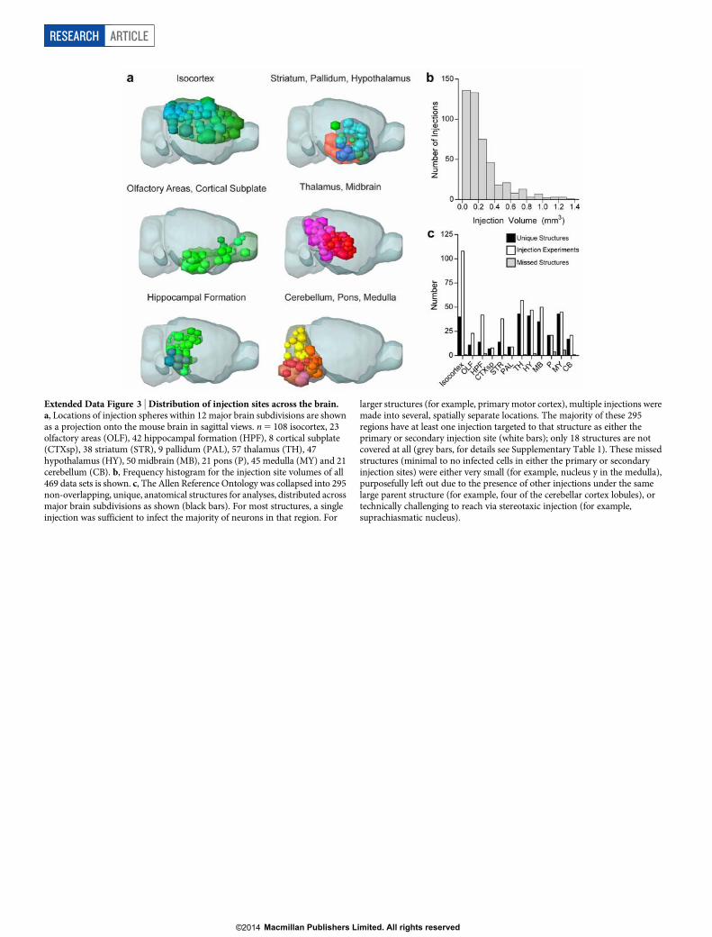
Extended Data Figure 3 | Distribution of injection sites across the brain.a, Locations of injection spheres within 12 major brain subdivisions are shownas a projection onto the mouse brain in sagittal views. n 5 108 isocortex, 23olfactory areas (OLF), 42 hippocampal formation (HPF), 8 cortical subplate(CTXsp), 38 striatum (STR), 9 pallidum (PAL), 57 thalamus (TH), 47hypothalamus (HY), 50 midbrain (MB), 21 pons (P), 45 medulla (MY) and 21cerebellum (CB). b, Frequency histogram for the injection site volumes of all469 data sets is shown. c, The Allen Reference Ontology was collapsed into 295non-overlapping, unique, anatomical structures for analyses, distributed acrossmajor brain subdivisions as shown (black bars). For most structures, a singleinjection was sufficient to infect the majority of neurons in that region. For

larger structures (for example, primary motor cortex), multiple injections weremade into several, spatially separate locations. The majority of these 295regions have at least one injection targeted to that structure as either theprimary or secondary injection site (white bars); only 18 structures are notcovered at all (grey bars, for details see Supplementary Table 1). These missedstructures (minimal to no infected cells in either the primary or secondaryinjection sites) were either very small (for example, nucleus y in the medulla),purposefully left out due to the presence of other injections under the samelarge parent structure (for example, four of the cerebellar cortex lobules), ortechnically challenging to reach via stereotaxic injection (for example,suprachiasmatic nucleus).

RESEARCH ARTICLE

Macmillan Publishers Limited. All rights reserved©2014

Extended Data Figure 4 | Distribution of whole brain projections fromdifferent cortical source areas. Pie charts show the percentage of totalprojection volume across all voxels outside of the injection site distributed inthe 12 major brain subdivisions from both hemispheres. Each pie chartrepresents the average of 4 to 27 cortical injections grouped by the broadregions listed. A pie chart key of the volume distribution (number of voxels perstructure/total number of voxels per brain) of these 12 subdivisions is at thebottom right for comparison. The largest projection signal from each corticalinjection is found within isocortex (range of 45.4–69.8% of projection signals

depending on source region, with an average of 59% for all cortical injections),although the isocortex accounts for only 30.2% of total brain volume.Differences in the subcortical distribution of relative signal strength betweencortical sources were also observed. For example, within the striatum (lightblue), the percentage of total signal is low from auditory, retrosplenial andvisual areas (6.2%, 3.4% and 7.6%, respectively), but much greater from frontal,motor, cingulate and somatosensory areas (16.5%, 27.7%, 20.3% and 17.6%,respectively).

ARTICLE RESEARCH

Macmillan Publishers Limited. All rights reserved©2014

Extended Data Figure 5 | Variability of brain-wide projection signalstrength. To examine animal-to-animal variability in projection patterns,12 sources with two spatially overlapping injection experiments were identifiedfrom the full data set of tracer injections shown in Fig. 3. a, Rows showsegmented projection volumes normalized to the injection volume(log10-transformed) in the 295 ipsilateral target regions for each of 2 individualoverlapping tracer injections per source region indicated (above and belowsolid black line). The colour map is as shown in Fig. 3. b, Maximal densityprojections of whole brain signals from each of the two spatially overlappinginjection experiments per source region visibly demonstrate consistency ofbrain-wide connections. Scatter plots of all ipsilateral and contralateral targetstructure values above a minimum threshold in both members of the pair(log10 5 23.5; non-blue values from a) show significant correlations betweeneach pair of injections across a four orders of magnitude range of projection

strengths. Values in the scatter plots are Pearson’s correlation coefficients (r).Note that in some cases (for example, PTLp) axon pathways appear to belabelled in only one of the pair. This could be due to random differences in theproportion of corticospinal projecting neurons labelled in a particular injectionwithin the same source area. Signal in large annotated white matter tractsare computationally removed from the connectivity matrix, and thus notincluded in the scatter plots. c, Detected fluorescent signals from each of twoinjections into the same location of primary somatosensory cortex registeredand overlaid with the average template brain (grey). Lower 2 rows, 2D rawimages from each injection experiment at different anterior-posterior levels.The centres of these injection sites are in the far left panel and their majortargets are in the right panels. See Supplementary Table 1 for the correspondingfull name and acronym for each region.

RESEARCH ARTICLE

Macmillan Publishers Limited. All rights reserved©2014

Extended Data Figure 6 | Cytoplasmic EGFP and synaptophysin-EGFPAAV tracer comparison, using primary motor cortex (MOp) injections asan example. a–f, Two-photon images showing an example of the labellingobtained using the Phase I virus for whole-brain projection mapping, whichconsists of a human Synapsin I promoter driving expression of EGFP. g–l, Tocompare cytoplasmic labelling of projections and identification of terminalregions with a presynaptic reporter virus, we made a construct with the samehSynapsin promoter driving expression of a triple reporter cassette (AAV2/1.pSynI.nls-hrGFP-T2A-tagRFP-T2A-sypGFP.WPRE.bGH): a nuclearlocalization signal attached to humanized Renilla GFP (nls-hrGFP), a T2Asequence followed by cytoplasmic tagRFP, a second T2A sequence, and thesynaptophysin-EGFP fusion (sypGFP). Owing to the two-photon imagingwavelength used (925 nm), the tagRFP (red) signal is weak to non-existent inthese images. a, g, An image at the centre of the infected area after injection intothe same region of MOp with the Phase I cytoplasmic viral tracer (a) andthe nuclear and synaptic reporter viral tracer (g). Examples of viral labelling inthe caudoputamen (b, h), somatosensory cortex (c, i), thalamus (d, j), pontinegrey (e, k) and inferior olivary complex in the medulla (f, l) are shown forboth tracers. The cytoplasmic viral tracer labels axons, revealing densebranching patterns in presumed terminal zones. The presynaptic reportervirus predominantly shows a punctate pattern of labelling consistent withpresynaptic protein expression patterns, and indicative of terminal zones.

Punctate or diffuse labelling was observed with the synaptic reporter virus innearly all MOp target regions manually and computationally identified usingthe cytoplasmic reporter, including those with both large and small signals.Fluorescent signal originating in fibres outside of large white matter tracts areincluded in the signal quantification and matrix shown in Fig. 3, but signalsfrom these large annotated fibre tracts are computationally removed.m–p, High-resolution images of terminal zones in the somatosensory cortex(m) and thalamus (o) identified using the cytoplasmic viral tracer show axonramification and punctate structures consistent with bouton labelling,similar to the synaptic reporter in the corresponding regions (n, p).q–r’, To validate the presynaptic expression of the sypGFP fusion protein,sections including and adjacent to the thalamic region shown in j were collectedafter two-photon imaging and immunostained with antibodies against GFP(chicken polyclonal 1:500, Aves Labs, Inc. #GFP-1020) and synapsin I(rabbit polyclonal, 1:200, Millipore, #AB1543P) or GFP (rabbit polyclonal,Life Technologies, #A-11122) and SV2 (mouse monoclonal, DSHB,SV2-supernatant) presynaptic proteins. q, r, Confocal images at a single planeshow punctate labelling indicative of presynaptic boutons for both sypGFP andsynapsin or SV2. Many puncta were colocalized (yellow arrows show selectexamples in q’ and r’), although quantification was not reliable due to the veryhigh density of presynaptic labelling by anti-Synapsin and anti-SV2.

ARTICLE RESEARCH

Macmillan Publishers Limited. All rights reserved©2014

Extended Data Figure 7 | Distribution of log10-transformed normalizedprojection volumes from the entire matrix presented in Fig. 3. The values(left-hand y axis, black bars) were number of target regions and derivedfrom Supplementary Table 2. The entire range of the normalized projectionvolumes in this matrix was between log10 5 214 and log10 5 1.5, and it peakedbetween log10 5 23.5 and log10 5 23.0. A manual analysis of true positive andtrue negative signals from 20 randomly chosen injection experiments,representing the range of injection sizes, was used to estimate the false positiverate at different threshold levels, shown on the right-hand y axis (grey circles).True positive values predominantly fall within the range of log10 5 24 to 1.5.For example, at a threshold of log10 5 24, the false positive rate was 27%,dropping to 14.5% at log10 5 23.5. False positives were almost exclusively dueto small segmentation artefacts in areas without actual fluorescently labelledaxon fibres.

RESEARCH ARTICLE

Macmillan Publishers Limited. All rights reserved©2014

Extended Data Figure 8 | Cortical domains identified by clustering analysisof projection patterns. Eighty injections were used in the analysis for whichthe injection site is strictly within the isocortex and injection volume.0.07 mm3. a, Scatter plot of the voxel densities (excluding injection sites) ofthe whole brains from two nearby anterior cingulate injections (ACAd andACAv) shows a strong correlation between the two (Spearman’s r5 0.82),whereas that of two distant injections (ACAd and SSp-m) shows littlecorrelation (r5 20.03). b, Hierarchical clustering of the projection patternbased on Spearman’s rank correlation coefficient of voxel density over the

entire brain. The pseudo-F statistics measures the coherence of clusters and isthe ratio of mean sum of squares between groups to the mean sum of squareswithin group. Peaks in the pseudo-F statistics (for example, at n 5 3, 8 and 21clusters) are indicators of greater cluster separation. For n 5 21 clusters, asystematic colour-code is given to each cluster to provide a visual guide to theircortical location (Fig. 5a), the numbers in parentheses indicate the number ofinjections in each group. c, Voxel densities from the 21 selected injections fromFig. 5a are overlaid as ‘dotograms’ at 8 coronal levels for the contralateralhemisphere.

ARTICLE RESEARCH

Macmillan Publishers Limited. All rights reserved©2014

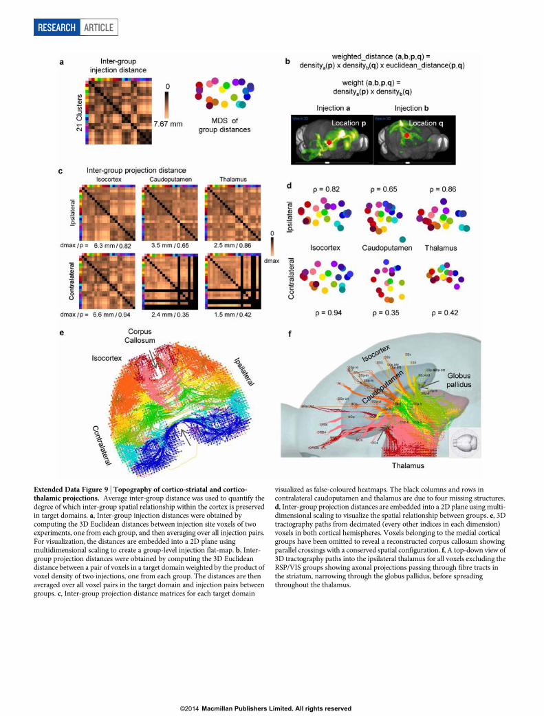
Extended Data Figure 9 | Topography of cortico-striatal and cortico-thalamic projections. Average inter-group distance was used to quantify thedegree of which inter-group spatial relationship within the cortex is preservedin target domains. a, Inter-group injection distances were obtained bycomputing the 3D Euclidean distances between injection site voxels of twoexperiments, one from each group, and then averaging over all injection pairs.For visualization, the distances are embedded into a 2D plane usingmultidimensional scaling to create a group-level injection flat-map. b, Inter-group projection distances were obtained by computing the 3D Euclideandistance between a pair of voxels in a target domain weighted by the product ofvoxel density of two injections, one from each group. The distances are thenaveraged over all voxel pairs in the target domain and injection pairs betweengroups. c, Inter-group projection distance matrices for each target domain

visualized as false-coloured heatmaps. The black columns and rows incontralateral caudoputamen and thalamus are due to four missing structures.d, Inter-group projection distances are embedded into a 2D plane using multi-dimensional scaling to visualize the spatial relationship between groups. e, 3Dtractography paths from decimated (every other indices in each dimension)voxels in both cortical hemispheres. Voxels belonging to the medial corticalgroups have been omitted to reveal a reconstructed corpus callosum showingparallel crossings with a conserved spatial configuration. f, A top-down view of3D tractography paths into the ipsilateral thalamus for all voxels excluding theRSP/VIS groups showing axonal projections passing through fibre tracts inthe striatum, narrowing through the globus pallidus, before spreadingthroughout the thalamus.

RESEARCH ARTICLE

Macmillan Publishers Limited. All rights reserved©2014

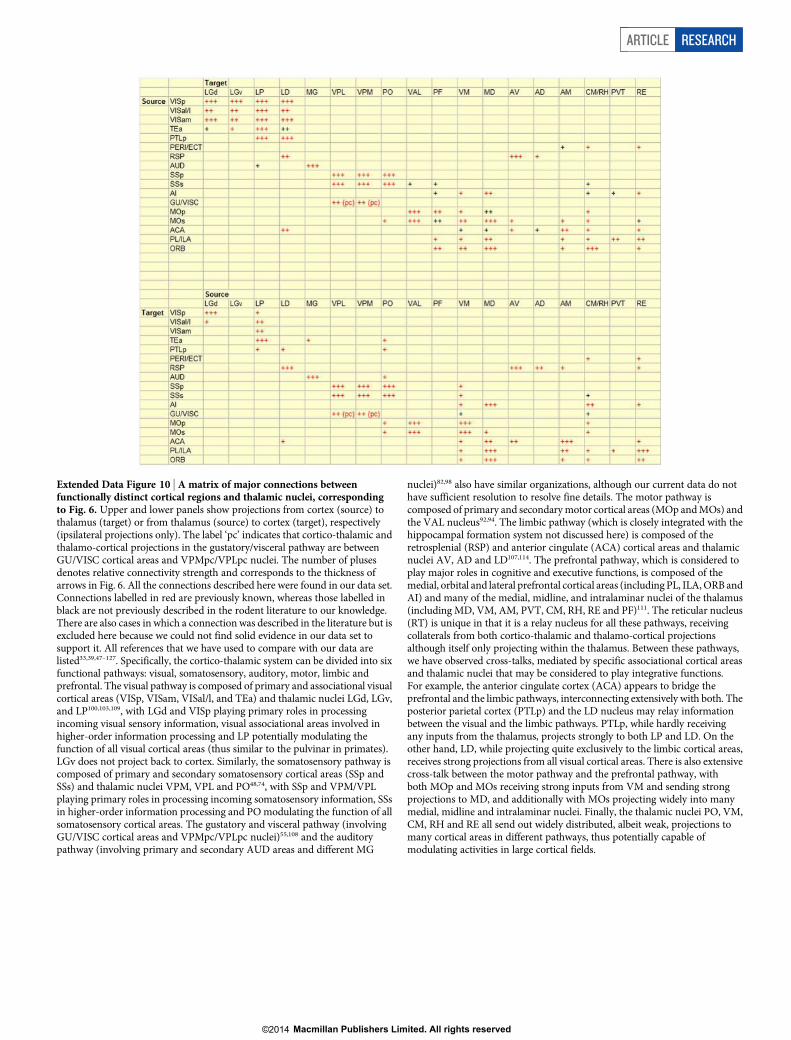
Extended Data Figure 10 | A matrix of major connections betweenfunctionally distinct cortical regions and thalamic nuclei, correspondingto Fig. 6. Upper and lower panels show projections from cortex (source) tothalamus (target) or from thalamus (source) to cortex (target), respectively(ipsilateral projections only). The label ‘pc’ indicates that cortico-thalamic andthalamo-cortical projections in the gustatory/visceral pathway are betweenGU/VISC cortical areas and VPMpc/VPLpc nuclei. The number of plusesdenotes relative connectivity strength and corresponds to the thickness ofarrows in Fig. 6. All the connections described here were found in our data set.Connections labelled in red are previously known, whereas those labelled inblack are not previously described in the rodent literature to our knowledge.There are also cases in which a connection was described in the literature but isexcluded here because we could not find solid evidence in our data set tosupport it. All references that we have used to compare with our data arelisted33,39,47–127. Specifically, the cortico-thalamic system can be divided into sixfunctional pathways: visual, somatosensory, auditory, motor, limbic andprefrontal. The visual pathway is composed of primary and associational visualcortical areas (VISp, VISam, VISal/l, and TEa) and thalamic nuclei LGd, LGv,and LP100,103,109, with LGd and VISp playing primary roles in processingincoming visual sensory information, visual associational areas involved inhigher-order information processing and LP potentially modulating thefunction of all visual cortical areas (thus similar to the pulvinar in primates).LGv does not project back to cortex. Similarly, the somatosensory pathway iscomposed of primary and secondary somatosensory cortical areas (SSp andSSs) and thalamic nuclei VPM, VPL and PO48,74, with SSp and VPM/VPLplaying primary roles in processing incoming somatosensory information, SSsin higher-order information processing and PO modulating the function of allsomatosensory cortical areas. The gustatory and visceral pathway (involvingGU/VISC cortical areas and VPMpc/VPLpc nuclei)55,108 and the auditorypathway (involving primary and secondary AUD areas and different MG

nuclei)82,98 also have similar organizations, although our current data do nothave sufficient resolution to resolve fine details. The motor pathway iscomposed of primary and secondary motor cortical areas (MOp and MOs) andthe VAL nucleus92,94. The limbic pathway (which is closely integrated with thehippocampal formation system not discussed here) is composed of theretrosplenial (RSP) and anterior cingulate (ACA) cortical areas and thalamicnuclei AV, AD and LD107,114. The prefrontal pathway, which is considered toplay major roles in cognitive and executive functions, is composed of themedial, orbital and lateral prefrontal cortical areas (including PL, ILA, ORB andAI) and many of the medial, midline, and intralaminar nuclei of the thalamus(including MD, VM, AM, PVT, CM, RH, RE and PF)111. The reticular nucleus(RT) is unique in that it is a relay nucleus for all these pathways, receivingcollaterals from both cortico-thalamic and thalamo-cortical projectionsalthough itself only projecting within the thalamus. Between these pathways,we have observed cross-talks, mediated by specific associational cortical areasand thalamic nuclei that may be considered to play integrative functions.For example, the anterior cingulate cortex (ACA) appears to bridge theprefrontal and the limbic pathways, interconnecting extensively with both. Theposterior parietal cortex (PTLp) and the LD nucleus may relay informationbetween the visual and the limbic pathways. PTLp, while hardly receivingany inputs from the thalamus, projects strongly to both LP and LD. On theother hand, LD, while projecting quite exclusively to the limbic cortical areas,receives strong projections from all visual cortical areas. There is also extensivecross-talk between the motor pathway and the prefrontal pathway, withboth MOp and MOs receiving strong inputs from VM and sending strongprojections to MD, and additionally with MOs projecting widely into manymedial, midline and intralaminar nuclei. Finally, the thalamic nuclei PO, VM,CM, RH and RE all send out widely distributed, albeit weak, projections tomany cortical areas in different pathways, thus potentially capable ofmodulating activities in large cortical fields.

ARTICLE RESEARCH

Macmillan Publishers Limited. All rights reserved©2014