A Meditation on Mediation:

Evidence That Structural Equations Models Perform Better Than Regressions

2

A Meditation on Mediation:

Evidence That Structural Equations Models Perform Better Than Regressions

In this paper, we suggest ways to improve mediation analysis practice among consumer

behavior researchers. We review the current methodology and demonstrate the superiority of

structural equations modeling, both for assessing the classic mediation questions, and for

enabling researchers to extend beyond these basic inquiries. A series of simulations are

presented to support the claim that the approach is superior. In addition to statistical

demonstrations, logical arguments are presented, particularly regarding the introduction of a

fourth construct into the mediation system. We close with new prescriptive instructions for

mediation analyses.

3

A Meditation on Mediation:

Evidence That Structural Equations Models Perform Better Than Regressions

Mediation is frequently of interest to social science researchers. A theoretical premise

posits that an intervening variable is an indicative measure of the process through which an

independent variable is thought to impact a dependent variable. The researcher seeks to assess

the extent to which the effect of the independent variable on the dependent variable is direct or

indirect via the mediator.

As depicted in Figure 1, X is the independent variable, M the hypothesized mediator, and

Y the dependent variable. For example, X might be a trait (e.g., need for cognition), M, a general

attitude (e.g., attitude toward a brand), and Y, a specific response judgment (e.g., likelihood to

purchase). Alternatively, X might be a mood induction, M, a cognitive assessment, and Y, a

memory test of previously exposed stimuli. Whatever the theoretical content, tests of mediation

are appealing to behavioral researchers attempting to track the process by which the X is thought

to impact the Y.

The basic approach to testing for empirical evidence of mediation was presented by

Baron and Kenny (1986) and Sobel (1982), and we will describe these methods shortly.

Building on this basic foundation, there is a small “mediation literature.” Some researchers have

expressed caution about the interpretation of causality in such correlational structures (e.g.,

Holland 1986, James and Brett 1984, James, Mulaik, and Brett 1982, McDonald 2002), some

arguing that experimental methods still reign supreme in the establishment of causality (e.g.,

Shrout and Bolger 2002, Spencer, Zanna and Fong 2005). Some researchers have tried to

improve upon the basic methods (e.g., Kenny, Kashy and Bolger 1998, MacKinnon et al. 2002,

4

MacKinnon, Warsi and Dwyer 1995). And some researchers have tackled both the causal logical

issues and the concerns regarding empirical improvements (e.g., Bentler 2001, Cote 2001,

Lehmann 2001, McDonald 2001, Netemeyer 2001). We will address all of these topics.

This paper is intended to guide researchers testing for evidence of mediation in frequently

encountered scenarios which are more complicated than those addressed in the foundational

article that appeared 20 years ago. First is the scenario in which a researcher has multiple

indicators of the X, M, and/or Y constructs—a scenario prefigured by Baron and Kenny (1986),

but not addressed fully in their article. Second is the scenario in which the X, M, and Y

constructs are themselves embedded in a richer nomological network that contains additional

antecedent and/or consequential constructs. In the final part of this paper, we build further on

these models, extending them to revisit a consideration from the 1986 article on moderated

mediation.

We will briefly review those regression procedures for testing for mediation patterns in

data, and illustrate that there is now a better alternative than what is common practice. While

some researchers have advocated (cf. Brown 1997; Preacher and Hayes 2004) and others

implemented (e.g., Mattanah, Hancock and Brand 2004) the use of structural equations models

for mediations, the point needs to be made that they are not merely an alternative to the

regressions—they should supplant the regressions. We offer empirical evidence of the

superiority of the structural equations modeling approach. These demonstrations are conducted

via simulation studies, in which the data qualities are known, so as to competitively assess the

performance of the standard approach with the structural modeling approach. This evidence has

been thus far lacking in the literature, so while other scholars have spoken up on behalf of

structural equations models, the typical user is left with the impression that structural equations

5

are merely an alternative to the extant regression techniques, and that either approach would be

sufficient and interchangeable in the inquiry. The simulations will indicate that even in the

simplest data scenarios, structural equations are a superior technology to regressions, and so

should always be used.

This paper is structured as follows. First we consider some common considerations that

arise as social scientists approach the question of mediation. We do so in the context of a

content analysis of recent years of consumer behavior research articles. These conceptual

concerns arise whether one were to conduct a mediation analysis via regression or structural

equations models. We then review the regression technique, and point to its shortcomings. We

present simulation studies to compare regressions to structural equations models on a number of

commonly encountered criteria, and close the paper with prescriptive advice for the researcher

looking to implement this newer technique.

Mediation Issues that Arise in the Literature

As Figure 2 indicates, mediation tests are frequently and increasingly reported in the

Journal of Consumer Psychology and the Journal of Consumer Research (reported in

approximately one quarter of the published articles). In this paper, we seek to make several

conceptual and empirical points, and we will refer to the JCP and JCR articles to make several of

these points. We will make reference in aggregate, as our goal is not to critique any particular

authors’ methodologies, rather to highlight several ways that the analytic and reporting practices

might be improved.

One question is whether all of these mediation examinations were necessary. For

example, in 72.3% of those articles, the introduction sections do not presage that the research

6

contained therein will examine the means by which X might impact Y, nor specifically that

mediation tests will be conducted. We do not mean to imply that an introduction section of a

paper must foreshadow all elements of the research inquiry, however, given the seemingly less

than central role of the mediation question, the mediation tests typically appear to be a

theoretically afterthought. The after-the-fact inclusion also raises the statistical concern of

capitalizing on chance in such post hoc tests.

In addition, the language researchers use to summarize this trivariate relationship

suggests a temporal or causal ordering (Holland 1986; James, Mulaik and Brett 1982), but

consider the fact that in 71.1% of those articles, the measures of X, M, and Y are either taken out

of order or simultaneously. For example, most researchers would agree that in a lab study, it is

good practice to measure the dependent variable first (to obtain a measure uncontaminated by

possible carry-over effects of other scales), and subsequently pose related attitude and covariate-

like questions to the respondent. It wouldn’t be unusual to see a study in which Y (say,

willingness to purchase) were measured first, followed by X (say attitude to the ad) and M

(attitude to the brand). When all three measures are items or scales that appear on a single

survey, the researcher bears the burden of arguing the ordered relationship on logical or

theoretical grounds. This goal is not unachievable (nor is the criticism of attempting to extract

causal statements from cross-sectional observational data novel), however rarely do researchers

attempt to follow the rigorous sequential data collection requirements to strengthen their

arguments (e.g., it is logistically challenging, some participant mortality may result, etc.). In

some circumstances, order might not be critical, e.g., if X were a stable demographic or trait

variable, it could be measured at the end of a survey without any concern of reactance; i.e., that

the measures of attitudes (M) or behaviors (Y) would have had an impact on the measure of a

7

pre-existing state, X. Yet when X, M, and Y all comprise attitudinal measures, and they are taken

out of order, it strains incredulity regarding the conceptual arguments.

Another common practice (i.e., appearing in 58.8% of the papers) is to use as M a

manipulation check of the experimental intervention, X (e.g., perhaps X is a manipulation of the

cognitive complexity of an ad and M is a measure of accuracy or speed on a performance test). It

does not seem to be a huge conceptual advance to the literature if one posits X to be some

theoretical construct and M merely its measurement; nor would such a demonstration represent

mediation as it is typically conceptualized.

As a final logical consideration prior to our illustrating the statistical issues, consider the

fact that for the “micro” social sciences (e.g., much of consumer behavior, psychology, etc.,

compared with sociology or macro economics), we have the luxury of conducting experiments;

universally acknowledged as the cleanest, surest methodological device for identifying causal

relationships. When researchers conduct a 2x2 experiment and use analysis of variance to test

the results, the paper is as strong as it can be. (This is not to say that studies aren’t designed with

flaws, but when true, the mediation analyses would be as problematic as the anovas.) It is

conceivable that a researcher believes he or she is adding value or rigor by introducing additional

statistical tests (i.e., indices associated with running the mediation analyses), but when the

researcher tacks on a mediation analysis, they are analyzing correlational data, which never have

the superiority for cleanly identifying causal premises. Thus the addition of mediation analyses

after reporting anovas on the central dependent variables dilutes, not strengthens, the paper.1

Let us begin by reviewing the basic regression technique. This approach is a combination

1 Spencer, Zanna and Fong (2005) argue that the chain of causality should be tested in a series of experimental studies—that the only possible concern is if the mediator is easier to measure than manipulate. Note however, this should not be a problem if the measured and manipulated variants of the mediator are purportedly tapping the same construct.

8

of the Baron and Kenny (1986) regressions and the Sobel (1982) follow-up z-test.

The Classic Mediation Test

Without question, the most popular means of testing for mediation is the procedure

offered by Baron and Kenny (1986). Using their approach, the researcher fits three regression

models:

11 εβ ++= aXM (1)

22 εβ ++= cXY (2)

33 ' εβ +++= bMXcY (3)

where the betas are the intercepts, the epsilons are the model fit errors, and the a, b, c, and c’

terms are the regression coefficients capturing the relationships between the three focal variables.

Evidence for mediation is said to be likely if:

1) the term a in equation (1) is significant; that is, there is evidence of a linear

relationship between the independent variable (X) and the mediator (M);

2) The regression coefficient c in equation (2) is significant; there is a linear relationship

between the independent variable (X) and the dependent variable (Y);2

3) The term b in equation (3) is significant, indicating that the mediator (M) helps predict

the dependent variable (Y), and also: c’, the effect of the independent variable (X)

directly on the dependent variable (Y), becomes significantly smaller in size relative to

c in equation (2).

2 This path, X Y is intuitively appealing, i.e., addressing the question, “is there any variance in Y explained by X, whether it will be shown to be indirect, or direct? However, since 1986 it has become somewhat controversial, with critics arguing that should the mediation be complete, e.g., all variance going from X to Y through M (or multiple Ms) then the direct path may be properly insignificant. For more on this issue, see James, Mulaik and Brett 2006; Kenny, Kashy and Bolger 1998; Shrout and Bolger 2002.

9

That last component, the comparison of size between c in (2) and c’ in (3) is conducted by the z-

test, 2222ba sasb

baz+

×= (Sobel 1982), where a and obtain from equation (1), and b and

from (3).

2as 2

bs

3

If either a or b is not significant, there is said to be no mediation. If (1), (2), and (3) hold,

the researcher would conclude there is “partial mediation.” If (1), (2), and (3) hold, and c’ is not

significantly different from zero, the effect is said to be perfect or complete mediation.4

In the articles we examined, the analytical details of mediation tests were often not fully

reported, but if we give authors the benefit of the doubt, we can report that 67.4% of the

mediation tests followed steps (1) through (3) properly.5 Yet fully 89.7% of the analyses did not

complete the z-test. When these tests were conducted, in 61.0% of the articles, the conclusion of

“partial mediation” was the result. While this status seems to be a sensible benchmark (i.e.,

some of the variance in Y explained by X is direct, and some is indirect through the mechanism

M), it is nevertheless somewhat unexciting or nondefinitive.

The Baron and Kenny (1986) article has been enormously influential both in shaping how

researchers think about mediation and in providing procedures to detect mediation patterns in

data. The citations for their article exceed 6000 and continue to climb. Most methodological

research fostered by the article has built on their basic logic. For example, MacKinnon and

colleagues have conducted methodological tests comparing alternative statistics with respect to

their relative power in detecting mediation patterns, as well as the comparative utility of rival

3 It can be shown that testing the difference between c (the direct effect), and c’ (the direct effect after controlling for the indirect, mediated effect) is equivalent to testing whether the strength of the mediated path (a x b) exceeds zero. 4 It has been suggested that rather than summarizing mediation analyses as one of three categorical results (i.e., none, partial, or full), it would be more informative to create a continuous index of the proportion of the variance in Y due to the indirect mediated path (Lehmann 2001; Mackinnon, Warsi and Dwyer 1995), an index we use later in the paper. 5 It is worth noting that this somewhat low percentage is indicative not only of consumer research but also of psychological research as well. Further, these issues should concern reviewers as well as authors.

10

indices expressing the extent to which a mediation structure is present in data (MacKinnon et al.

2002; MacKinnon et al. 1995; www.public.asu.edu/~davidpm/ripl/mediate.htm).

Part I: Measurement—Incorporating Multiple Indicators of X, M, and/or Y

Social science data subjected to mediation analysis are usually obtained from human

respondents and thus estimations of statistical relationships will be attenuated due to

measurement error. Baron and Kenny (1986, p.1177) acknowledge that, like any regression,

their basic approach makes no particular allowance for measurement error, which is simply

subsumed into the overall error term, contributing to the lack of fit, 1-R2. While it is true that

proceeding with a single variable as a sole indicator of a construct is statistically conservative

(see the argument recently revived by Drolet and Morrison 2001), most social scientists concur

in the view that multi-item scales are generally preferable, in philosophical accordance with

classical test theory and notions of reliability that more items comprise a stronger measurement

instrument.6 The 1986 procedures are applicable only to systems of three variables, i.e., only one

indicator measure per each of the three constructs, yet Figure 3 illustrates a typical research

investigation which provides for multi-item scales for each of the focal constructs. The figure is

merely an example; for the techniques to be described, the number of items may be two or more,

for each of X, M, and Y (and the number of items per construct need not be equal).

It is perhaps easiest to envision the scenario in which there exist multiple predictor

variables, X1, X2, X3, and a single mediator M and dependent variable Y. Equations (1)-(3) would

6 Baron and Kenny (1986, p.1177) state, “Generally the effect of measurement error is to attenuate the size of measures of association, the resulting estimate being closer to zero than it would be if there were no measurement error. [For example], measurement error in the mediator [only] is likely to result in an overestimate in the [direct] effect of the independent variable on the dependent variable.” Bracketed words were inserted for clarification, e.g., in contrast, if X and Y were measured with error but M were not, then the mediated path could loom larger than the direct path.

11

be replaced with the variants containing the multiple predictor variables:

43322114 εβ ++++= XaXaXaM (4)

53322115 εβ ++++= XcXcXcY (5)

63322116 ''' εβ +++++= bMXcXcXcY . (6)

However, even in this simple extension, the complicating issues become two: first, it is not clear

which coefficients should be compared to assess the extent of mediation, and second, the effects

of the multicollinearity among X1, X2, X3, which is inherent to predictors that represent multiple

indicators of a common construct, will clearly be debilitating.

The scenario becomes even more complex should the mediator M or the dependent

variable Y be measured with more than one item. At first, it might seem that the new

complexities would be simply analogous to those for X. However, M and Y each serve as

dependent variables in the series of mediation regressions, hence a proliferation of M’s or Y’s

will require more predictive equations, for example, three mediators and two dependent variables

would yield:

733221171 εβ ++++= XaXaXaM (7)

833221182 εβ ++++= XaXaXaM (8)

933221193 εβ ++++= XaXaXaM (9)

10332211101 εβ ++++= XcXcXcY (10)

11332211112 εβ ++++= XcXcXcY (11)

121332211121 ''' εβ +++++= bMXcXcXcY (12)

132332211131 ''' εβ +++++= bMXcXcXcY (13)

143332211141 ''' εβ +++++= bMXcXcXcY (14)

12

151332211152 ''' εβ +++++= bMXcXcXcY (15)

162332211162 ''' εβ +++++= bMXcXcXcY (16)

173332211172 ''' εβ +++++= bMXcXcXcY . (17)

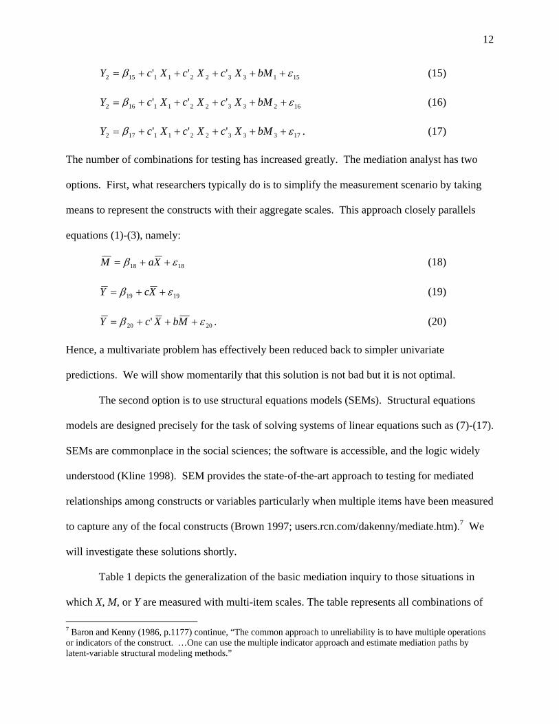
The number of combinations for testing has increased greatly. The mediation analyst has two

options. First, what researchers typically do is to simplify the measurement scenario by taking

means to represent the constructs with their aggregate scales. This approach closely parallels

equations (1)-(3), namely:

1818 εβ ++= XaM (18)

1919 εβ ++= XcY (19)

2020 ' εβ +++= MbXcY . (20)

Hence, a multivariate problem has effectively been reduced back to simpler univariate

predictions. We will show momentarily that this solution is not bad but it is not optimal.

The second option is to use structural equations models (SEMs). Structural equations

models are designed precisely for the task of solving systems of linear equations such as (7)-(17).

SEMs are commonplace in the social sciences; the software is accessible, and the logic widely

understood (Kline 1998). SEM provides the state-of-the-art approach to testing for mediated

relationships among constructs or variables particularly when multiple items have been measured

to capture any of the focal constructs (Brown 1997; users.rcn.com/dakenny/mediate.htm).7 We

will investigate these solutions shortly.

Table 1 depicts the generalization of the basic mediation inquiry to those situations in

which X, M, or Y are measured with multi-item scales. The table represents all combinations of

7 Baron and Kenny (1986, p.1177) continue, “The common approach to unreliability is to have multiple operations or indicators of the construct. …One can use the multiple indicator approach and estimate mediation paths by latent-variable structural modeling methods.”

13

single vs. multiple measures of X, M, and Y and illustrates those conditions for which a

regression approach may be used versus those conditions under which SEMs would be the

appropriate technique for examining mediation structures. Specifically, either the regression

technique or SEM techniques may be applied any time each of the X, M, and Y constructs are

represented by a single score,8 whether a single variable (e.g., M) or a scale composed of the

average of the items purporting to measure the construct (e.g., {M1, M2, M3} M ). However,

as we shall demonstrate, while there is some correspondence between the regression and SEM

approaches, the SEM technique is the superior method on both theoretical and empirical

statistical grounds. The other scenarios in Table 1 depict situations in which a researcher has

multiple items for X, M, or Y and wishes to model them as such rather than creating an aggregate

score. In these conditions, SEMs provides the natural choice for determining mediation

structures. We turn now to the methodological comparisons.

Study 1

To compare the analytical approaches, we created a series of Monte Carlo simulations to

investigate and compare the regression vs. SEM methodologies in terms of superiority in

identifying mediation structures. The strength of simulation studies is that the population

parameters are constructed, so the researcher knows the true relationship in a population, and the

logic is to investigate the extent to which the regressions or SEMs are capable of identifying and

recovering it properly.

In Study 1, we varied two properties: the strength of the mediated vs. direct effects in the

population, and the sample size in the data. For the first factor, we created conditions for full 8 If the constructs are measured via single items, the full structural equations model is called a “path model,” as there would be a structural component but the measurement model would default to the assumption of perfect measurement (as the regression assumes).

14

(100%) mediation, 75% of the variance in Y due to mediation through M, 50%, 25% and 0%

(i.e., no mediation, only a fully direct effect). The precise operationalization of these conditions

is described shortly. For now, we note that we have created clean conditions that either method

should identify (e.g., 100% or 0% mediation; that is, full or none), conditions that favor one

conclusion vs. another but not as precisely (i.e., 75% or 25% mediation), and conditions that

should be empirically challenging for any method, i.e., 50%, a partial mediation condition where

the variance is equally attributable to the direct and mediated paths. In sum, the factor, “%

mediation,” took on the levels: 100%, 75%, 50%, 25%, and 0%.

The second factor was sample size, and we examined n=30, 50, 100, 200, and 500. These

sample sizes seemed plausibly comprehensive in representing most published behavioral

research.

The factorial design was thus: 5 (%mediation = 100, 75, 50, 25, 0) x 5 (sample size n =

30, 50, 100, 200, 500). In these 25 experimental conditions, 1000 samples were generated with n

observations and p standard normal deviates. The population covariance matrix depicting the

extent of direct and indirect relationships among the three constructs was factored via a standard

Cholesky decomposition, and the resultant matrix multiplied by the p-variate independent

normals, i.e., MVNp(0,I) to create the proper inter-correlations, i.e., MVNp(0,Ε). In each sample,

mediation analyses were conducted to obtain the parameter estimates and fit statistics. Empirical

distributions were thus built with 1000 observations for estimates of the path coefficients, their

standard errors, a battery of fit indices, etc.

Results of Study 1

In comparing the performance of SEMs and regressions in this simplest data scenario

15

(i.e., one X, one M, and one Y), we note the techniques yield very similar results. The parameter

estimates themselves, i.e., the regression weights and the path coefficients, are identical. For

example, the reader can verify that the correlation matrix: rXM = 0.354, rXY = 0.375, rMY = 0.354

translates to path coefficients: a = 0.354, b = 0.253, c = 0.285, whether computed via the three-

step regression approach or via a single simultaneous structural equations model.9

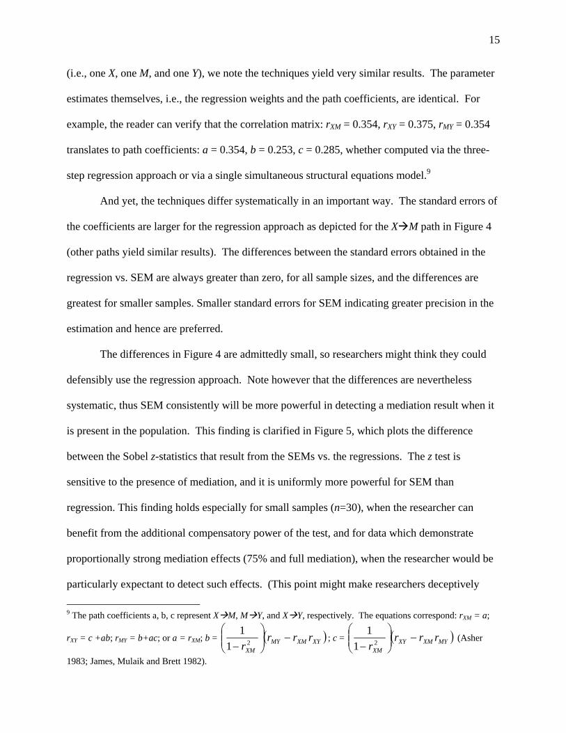
And yet, the techniques differ systematically in an important way. The standard errors of

the coefficients are larger for the regression approach as depicted for the X M path in Figure 4

(other paths yield similar results). The differences between the standard errors obtained in the

regression vs. SEM are always greater than zero, for all sample sizes, and the differences are

greatest for smaller samples. Smaller standard errors for SEM indicating greater precision in the

estimation and hence are preferred.

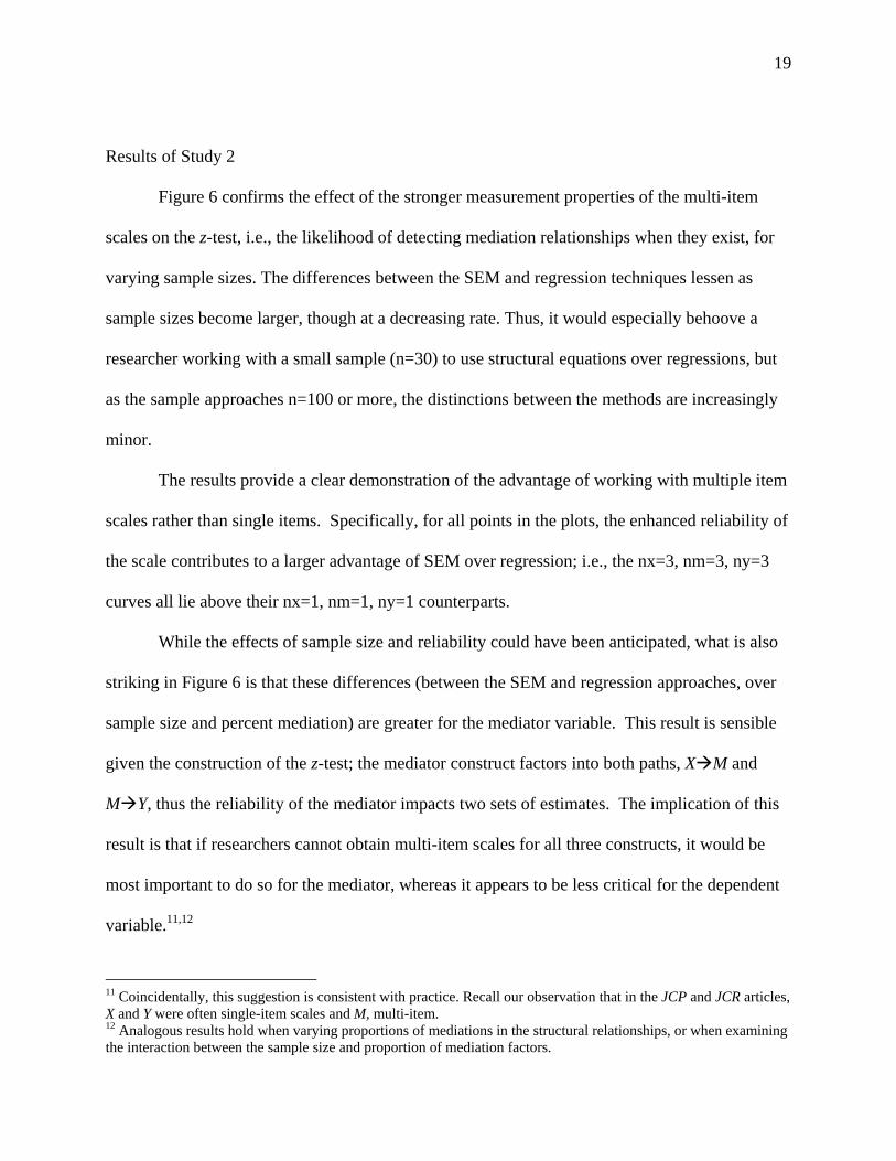
The differences in Figure 4 are admittedly small, so researchers might think they could

defensibly use the regression approach. Note however that the differences are nevertheless

systematic, thus SEM consistently will be more powerful in detecting a mediation result when it

is present in the population. This finding is clarified in Figure 5, which plots the difference

between the Sobel z-statistics that result from the SEMs vs. the regressions. The z test is

sensitive to the presence of mediation, and it is uniformly more powerful for SEM than

regression. This finding holds especially for small samples (n=30), when the researcher can

benefit from the additional compensatory power of the test, and for data which demonstrate

proportionally strong mediation effects (75% and full mediation), when the researcher would be

particularly expectant to detect such effects. (This point might make researchers deceptively

9 The path coefficients a, b, c represent X M, M Y, and X Y, respectively. The equations correspond: rXM = a;

rXY = c +ab; rMY = b+ac; or a = rXM; b = ( )XYXMMYXM

rrrr

−⎟⎟⎠

⎞⎜⎜⎝

⎛− 21

1; c = ( )MYXMXY

XM

rrrr

−⎟⎟⎠

⎞⎜⎜⎝

⎛− 21

1 (Asher

1983; James, Mulaik and Brett 1982).

16

confident that the regression approach is at least “conservative.” However, our results will

demonstrate that the regression results are misleading, and the SEM results are closer to the

truth, the population parameters.)

The (slight) advantage of SEM over regression is due to the fact that the standard errors

in the SEM approach are reduced, in turn because of the simultaneous estimation of all

parameters in the SEM model. Fitting components of models simultaneously is always

statistically superior to doing so in a piece-meal fashion, e.g., to statistically control for and

partial out other relationships. That is, the empirical results are not a coincidence or function of

the data, as they are driven by the statistical theory that the simultaneously fit equations will

dominate in producing more consistent estimates. Thus, both theoretically and empirically,

fitting a single SEM model lends more efficient and elegant estimation than the three regression

pieces. Note too, that when SEM is the tool used for mediation analyses, one model is fit. The

researcher does not fit a series of equations or models per the regression techniques of Baron and

Kenny (1986).

The follow-up z-test is still important, because even if the SEM model yielded path

coefficients from X M and M Y that were significant, and X Y that was not, if those

respective estimates were, say, 0.7, 0.6, 0.3, then the indirect paths might not be significantly

greater than the direct path (the aforementioned significance tests would indicate merely that 0.7

and 0.6 were greater than 0.0 and that 0.3 was not, but the z-test compares directly whether the

mediated path (0.7 x 0.6) exceeds the strengths of the direct path, 0.3). Note too that in fitting

one simultaneous model, all the parameters and standard errors (pieces of the z-test) are

estimated conditional upon the same effects being present in the model. Currently, the z-test is

formed after deriving those estimates from different models, for which the estimates are based

17

upon conditioning on different subsets of predictor variables (i.e., in sum, the regressions

compare apples to oranges; the structural equation model compares apples to apples).

It is also of some comfort that the structural equations models performed as well as they

did even with the smallest samples, n=30. Just as in applications of the general linear model,

researchers rarely consult power estimates, instead relying on rules of thumb for requisite sample

size, e.g., “n>200” in structural equations models. Our results suggest that those rules of thumb

are very conservative, at least for models with relatively few constructs, such as these considered

in mediation tests.

In conclusion, even in this simplest of data scenarios—the classic case of only three

constructs and only one measure per construct—the choice between regression and SEMs

matters, and structural equations modeling is the superior technology. The SEM results work to

the researcher’s benefit, in being more likely to detect existing patterns of mediation, being truer

to the known population structural characteristics, and finally in also being statistically more

defensible, given the elegance of the simultaneous estimation.

Study 2

The classic mediation scenario of one indicator measure per construct, X, M, and Y, is the

most frequently implemented. And yet of course, multiple measures per construct are easily

accommodated via the regression approach if scale averages are used, as X , M , and Y , per

equations (18) – (20).

In the articles published in JCP and JCR, the majority of studies used a single indicator

for X (83.7%) and Y (52.2%) but multi-item scales for M (57.8%). When multi-item scales were

used (for any of the three constructs), researchers aggregated to averages.

18

Reliability theory would predict that constructs measured with multi-item scales should

provide stronger results than those measured with single items, and the mediation context should

prove consistent in that regard. To verify, in this study we compare the model performance

across the eight conditions depicted in Table 1 in which both regressions and SEMs may be run,

specifically all combinations where there exists either a single item, or multiple items averaged

to form a scale measuring each construct.

Building on the design of Study 1, we continue with the factors of “%mediation” and

sample size, extending the investigation to the effects of single vs. multiple items measuring each

of X, M, and Y. We defined “multiple items” to be three indicators per construct.10 For the

multi-item scales conditions, we incorporated a level of reliability of 0.75 to exceed the

conventional rule of thumb of 0.7 (and yet to be fairly realistic in value). Thus, there were two

conditions for X (one-item X vs. an average of three-items, X based on X1, X2, X3 with

reliability Xα = 0.75), analogously for M (one-item M vs. M with Mα =0.75), and for Y (one-item

Y vs. Y , with Yα =0.75).

The full factorial design was thus: 5 (%mediation= 100, 75, 50, 25, 0) x 5 (sample size

n=30, 50, 100, 200, 500) x 2 (X or Xα =0.75) x 2 (M or Mα =0.75) x 2 (Y or Yα =0.75). In each of

these 5x5x23 = 200 experimental conditions, 1000 samples were generated, and mediation

analyses conducted to obtain the parameter estimates and fit statistics. These conditions allow

the comparison of the regression and SEM analytical approaches for which there exist either a

single measure, or a composite scale; i.e., X or X , M or M , Y or Y .

10 Clearly we could have varied this factor more extensively, examining two, four, five items, etc., but variations on reliability and scale length are well-known—specifically there will be enhanced reliability with longer scales, and the relationships between constructs measured with more items thus will appear stronger than those between constructs measured with shorter scales. Given that properties of reliability are well-documented in the literature, we pursued a single contrast, between one- and three-item scales.

19

Results of Study 2

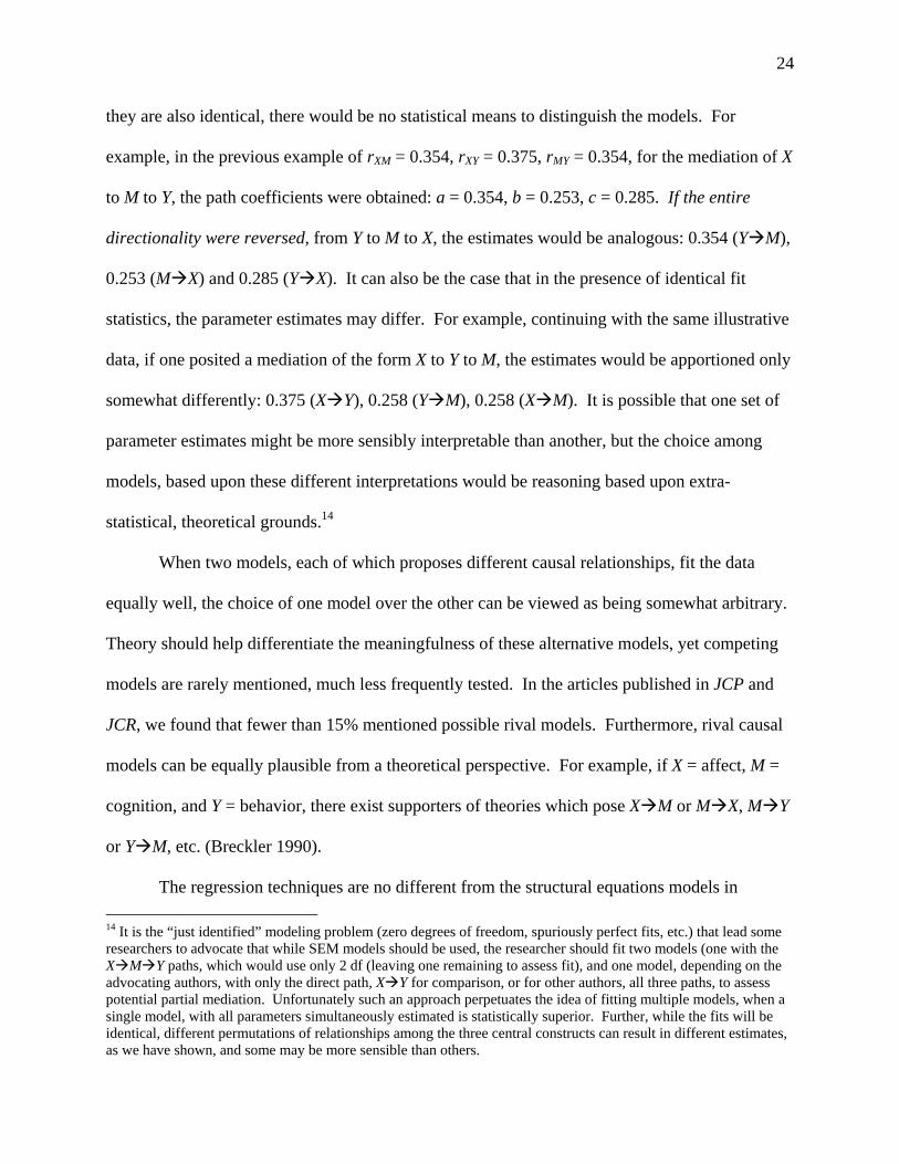
Figure 6 confirms the effect of the stronger measurement properties of the multi-item

scales on the z-test, i.e., the likelihood of detecting mediation relationships when they exist, for

varying sample sizes. The differences between the SEM and regression techniques lessen as

sample sizes become larger, though at a decreasing rate. Thus, it would especially behoove a

researcher working with a small sample (n=30) to use structural equations over regressions, but

as the sample approaches n=100 or more, the distinctions between the methods are increasingly

minor.

The results provide a clear demonstration of the advantage of working with multiple item

scales rather than single items. Specifically, for all points in the plots, the enhanced reliability of

the scale contributes to a larger advantage of SEM over regression; i.e., the nx=3, nm=3, ny=3

curves all lie above their nx=1, nm=1, ny=1 counterparts.

While the effects of sample size and reliability could have been anticipated, what is also

striking in Figure 6 is that these differences (between the SEM and regression approaches, over

sample size and percent mediation) are greater for the mediator variable. This result is sensible

given the construction of the z-test; the mediator construct factors into both paths, X M and

M Y, thus the reliability of the mediator impacts two sets of estimates. The implication of this

result is that if researchers cannot obtain multi-item scales for all three constructs, it would be

most important to do so for the mediator, whereas it appears to be less critical for the dependent

variable.11,12

11 Coincidentally, this suggestion is consistent with practice. Recall our observation that in the JCP and JCR articles, X and Y were often single-item scales and M, multi-item. 12 Analogous results hold when varying proportions of mediations in the structural relationships, or when examining the interaction between the sample size and proportion of mediation factors.

20

In conclusion, Study 2 demonstrates that when multi-item scales are aggregated and their

means imputed into regressions, the added reliability of a scale over a single item definitely

clarifies the obtained results. Orthogonal to that observation, the use of a structural equations

model is superior to the regressions, except for the techniques being equal when there exists no

mediation, or nearly equal if the sample size is large, n=500 (or perhaps n=200, but in either

event, substantially larger than is typically observed in the research studies in JCP and JCR that

seek to test for mediation).

There is no circumstance in which a structural equation is outperformed by the

regressions. Studies 1 and 2 have shown a consistent advantage of SEM over regression for

detecting mediation structures when they exist in data. Thus, we will focus on SEM for the

remainder of the paper, not just because of its demonstrable superiority, but also because we will

be examining scenarios where the application of regression would be difficult or impossible.

Study 3

Taking means over multiple items (e.g., {X1, X2, X3} X ) to simplify analyses (as

investigated in Study 2) is commonplace, but doing so does not use the data to their full

advantage as would allowing the representation of the items in a measurement model while

fitting the mediation structural model in a SEM. In this study, we compare multiple items for X,

M, and Y as used in SEM vs. their aggregate means. As in our previous studies, we factor in

effects for sample size and strength of mediation. Each construct is measured with multiple

items and an aggregate analysis (i.e., means as in Study 2) is compared to the use of a full

structural equations model (i.e., the inclusion of both the measurement and the path models).

Operationally, per the previous studies, samples of size n (again varying from 30 to 500)

21

were generated using the population covariance matrix constructed to reflect the strength of

mediation (i.e., 0, 25, 50, 75, 100%). For the “mean” treatment of these data, averages were

taken over X1, X2, X3 to obtain X ; M1, M2, M3 to obtain M ; and Y1, Y2, Y3 to obtain Y , resulting

in an analysis like that in Study 2, described in equations (18) through (20). For the “full SEM”

treatment of these data, measurement models posited X1, X2, X3 as three indicators of the

construct X; M1, M2, M3 as measures of M; and Y1, Y2, Y3 of Y, accordingly, and the mediation

structure was tested amongst the constructs, having explicitly modeled the measurement qualities

(rather than merely aggregating over the items).

Results of Study 3

We could present the standard errors and z-tests, as we have for Studies 1 and 2, but these

indices performed predictably (i.e., like those for Studies 1 and 2), hence for Study 3, we present

a different set of dependent variable results. The goal of this study is to compare how well

structural equations models perform on 3x3 covariance matrices of means, vs. 9x9 covariance

matrices of items modeled via measurement and path structures. One assessment of each

technique is whether the qualitative conclusion to which the researcher is led is indeed the proper

outcome. Specifically, for both the “mean” and “full SEM” treatments of these data, the Sobel z-

tests were computed, and the results for each of the 500 replicate samples in each condition

classified as “no,” “partial,” or “full” mediation, as a conclusion that a researcher would seek to

report.

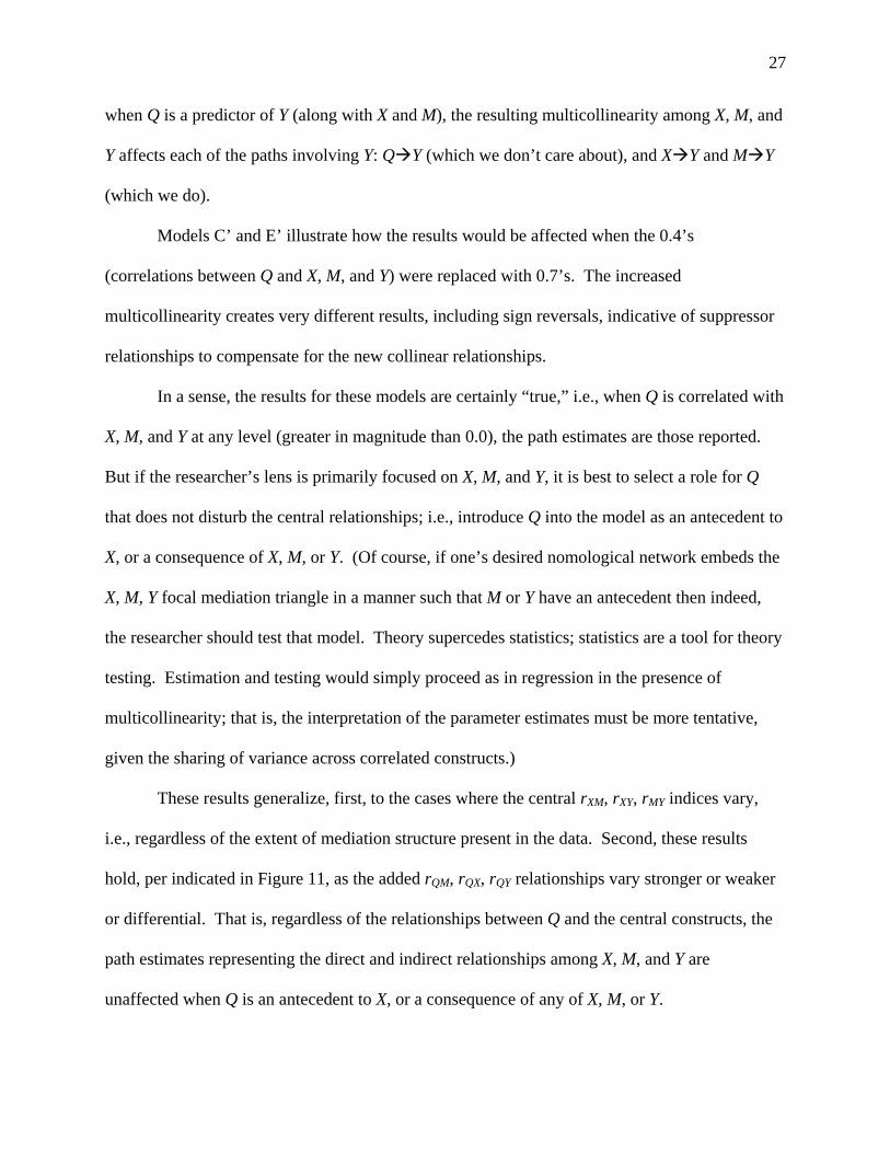
Figure 7 shows that when the mediation is in the state of “no,” “partial,” or “full,” and

identified as such by the “full SEM” model, there are misclassifications by the “mean” treatment

of these data. For example, when the full SEM model properly identifies “no mediation” (the

22

left two bars) the analysis of means comes to that same conclusion most frequently, but also

fairly often concludes incorrectly that there is full or partial mediation. For stronger mediation

effects, the proportions of misclassifications decline.13

Thus, the results for the analysis using mean scores for X, M, and Y deviate from the true

population relationships compared to the results from the full SEM treatment of the multi-item

data. When the researcher has multi-item scales (for X, M, or Y), averaging the scales, rather

than modeling them via SEM, does a disservice to the data. Within structural equations

modeling, it is important to let the data speak according to their inherent properties—if there are

three indicators of a construct, a properly isomorphic measurement model should be incorporated

simultaneously with the structural model seeking to test the mediation, rather than collapsing the

data to means. Aggregating might seem to simplify matters, but simplification in procedural and

analytical matters comes at the cost of inaccuracy in substantive and theoretical conclusions.

To summarize the findings of Part I, Studies 1 and 2 show that the choice between

regression and structural equations models matters, and that structural equations modeling is the

superior technology. Study 3 demonstrated that the short-cut of using mean scores for X, M, and

Y is inferior to representing measurement models fully via the SEM model.

We began the paper by discussing two directions in which mediation analyses might be

extended: first in terms of multiple measures, as we have been examining; and second, in terms

of introducing additional constructs. Thus, we now turn to Part II of this paper, and study

mediation in the context of a more complex nomological network.

Part II: Structural Analysis—Embedding the Focal Mediation in a Nomological Network

13 Given the concern previously raised, that the regression approach is not more conservative, but rather more errorful, it is important to note that when we include regressions as another benchmark, those classification results were somewhat worse than these cited for the Mean SEM, both of which are dominated by the Full SEM.

23

Researchers seeking to investigate mediation among the X, M, and Y constructs often

investigate these constructs with a relatively narrow lens that includes only those constructs (e.g.,

usually for purposes of efficiency, such as shorter experiments or surveys). However, all

construct relationships are implicitly embedded in a larger picture, such as that in Figure 8. This

broader nomological network is encouraged by philosophers of science and methodologists to

offer the richest view of the phenomena and their explanations (Cronbach and Meehl 1955).

Certainly a theoretical mapping as complex as that in Figure 8 cannot be achieved in a single

paper, nor would we insist upon such unrealistic goals. However, we wish to clarify that the

addition of at least one more construct, Q, is necessary even if the researcher cares more about X,

M, and Y than Q (Bentler 2001). Furthermore, we shall demonstrate that the role of Q is quite

specific.

The primary theoretical purpose of the introduction of at least one additional construct is

to make the nomological network more sophisticated, and therefore make the nature of the

results more statistically certain. The complexity enhances conceptual explanation, and makes

the positing of plausible rival theories for observed data patterns more difficult.

The principal statistical purpose of the additional construct is to yield sufficient degrees

of freedom to test the mediation links. The mediation model, which posits three links among

three constructs (to which we have been making most reference), may be characterized as “just

identified,” meaning that all degrees of freedom are used up in estimating the paths, which in

turn means that the directionality of the effects, from X to M vs. M to X is empirically

indeterminate (MacCallum et al. 1993; McDonald 2002). In the presence of zero degrees of

freedom, many models fit the data perfectly (e.g., CFI = 1.00; rmse = 0.00). Aside from the

omnibus model fit statistics, the parameter estimates themselves can be identical or different. If

24

they are also identical, there would be no statistical means to distinguish the models. For

example, in the previous example of rXM = 0.354, rXY = 0.375, rMY = 0.354, for the mediation of X

to M to Y, the path coefficients were obtained: a = 0.354, b = 0.253, c = 0.285. If the entire

directionality were reversed, from Y to M to X, the estimates would be analogous: 0.354 (Y M),

0.253 (M X) and 0.285 (Y X). It can also be the case that in the presence of identical fit

statistics, the parameter estimates may differ. For example, continuing with the same illustrative

data, if one posited a mediation of the form X to Y to M, the estimates would be apportioned only

somewhat differently: 0.375 (X Y), 0.258 (Y M), 0.258 (X M). It is possible that one set of

parameter estimates might be more sensibly interpretable than another, but the choice among

models, based upon these different interpretations would be reasoning based upon extra-

statistical, theoretical grounds.14

When two models, each of which proposes different causal relationships, fit the data

equally well, the choice of one model over the other can be viewed as being somewhat arbitrary.

Theory should help differentiate the meaningfulness of these alternative models, yet competing

models are rarely mentioned, much less frequently tested. In the articles published in JCP and

JCR, we found that fewer than 15% mentioned possible rival models. Furthermore, rival causal

models can be equally plausible from a theoretical perspective. For example, if X = affect, M =

cognition, and Y = behavior, there exist supporters of theories which pose X M or M X, M Y

or Y M, etc. (Breckler 1990).

The regression techniques are no different from the structural equations models in 14 It is the “just identified” modeling problem (zero degrees of freedom, spuriously perfect fits, etc.) that lead some researchers to advocate that while SEM models should be used, the researcher should fit two models (one with the X M Y paths, which would use only 2 df (leaving one remaining to assess fit), and one model, depending on the advocating authors, with only the direct path, X Y for comparison, or for other authors, all three paths, to assess potential partial mediation. Unfortunately such an approach perpetuates the idea of fitting multiple models, when a single model, with all parameters simultaneously estimated is statistically superior. Further, while the fits will be identical, different permutations of relationships among the three central constructs can result in different estimates, as we have shown, and some may be more sensible than others.

25

offering no solution to the issue of using all the available degrees of freedom in the

decomposition of the variance (recall the equivalence of the parameter estimates in Studies 1 and

2; fitting the model in regression pieces does not overcome the logical difficulties). The use of

multi-item scales (such as that investigated in Study 3) offers no solution to this problem

either—while the source covariance matrix is larger, the additional degrees of freedom are

“illusory,” in that they contribute to the measurement model accuracy, but they do not contribute

degrees of freedom to the critical structural model. With three constructs, there are three inter-

construct correlations, no matter the number of measured items, and three path estimates to

obtain—hence the “just identified” status. However, with four constructs, there are six

correlations. If four paths are estimated, two spare degrees of freedom are available to test the

superiority of competitive model fits. This scenario of “overdetermination” is preferred because

in the system of simultaneous equations, there are fewer unknowns than equations or

corresponding data points in the system, so each estimate may be obtained with more certainty.

Figure 9 presents all possible positions for a new construct Q, as an antecedent or

consequence relating to X, M, and Y, in turn. Each of these recursive, identified, structural

models achieves the goal of introducing degrees of freedom for assessing model fit (i.e., none of

the models is artifactually perfectly fit). However, we shall demonstrate that the six models are

not equivalent in status in solving concerns regarding the focal mediation testing, in particular,

models “C” and “E” should not be used, and after the following study, we conclude with

prescriptions as to optimal model form.

Study 4

This study demonstrates the effect of introducing a fourth construct, Q, into the extant

26

nomological network containing X, M, and Y. We can illustrate the effects of the introduction by

using the running example of rXM = 0.354, rXY = 0.375, rMY = 0.354. For the “baseline”

mediation model (that is, prior to the inclusion of Q), recall that the path coefficients were: a =

0.354, b = 0.253, c = 0.285. These estimates are presented in the upper right of Figure 10, for

“the baseline model”; i.e., mediation amongst only X, M, and Y, with no fourth construct, Q. For

comparison, the same correlations are supplemented with correlations between each of the

original constructs (X, M, and Y) and Q. This additional correlation is given an arbitrary value,

e.g., 0.40 in this illustration. When these data are fit to structural models A, B, D, and F, the

three focal path coefficient estimates remain unchanged (and the links involving Q as an

antecedent of X or a consequence of X, M, or Y, faithfully yield the input relation of 0.40).

Models C and E are presented in Figure 11. These two models behave differently

because the introduction of Q into the model as an antecedent to M or Y means there will be two

exogenous constructs (X and Q), which in turn brings a statistical (conceptual and empirical)

requirement that their correlation be represented and estimated. Thus, first, while models A, B,

D, and F (of Figure 10) carry two degrees of freedom, models C and E (in Figure 11) yield only

one (one degree of freedom is used in the estimation of the exogenous intercorrelation). That is

an unfortunate loss of degrees of freedom but not a catastrophic modeling problem.

However, the second problem introduced is more difficult: the three focal mediation path

coefficients are no longer invariant. In model C, when Q is a predictor of M (along with X), the

resulting multicollinearity between Q and X yields estimates that share the predictive variance,

hence, the Q M path is not 0.40 as input, but also, the X M path is no longer the 0.354 value

we’ve come to expect (as representing the known population structure). Note that the paths

involving the prediction of Y (i.e., M Y and X Y) are unaffected. Conversely, in model E,

27

when Q is a predictor of Y (along with X and M), the resulting multicollinearity among X, M, and

Y affects each of the paths involving Y: Q Y (which we don’t care about), and X Y and M Y

(which we do).

Models C’ and E’ illustrate how the results would be affected when the 0.4’s

(correlations between Q and X, M, and Y) were replaced with 0.7’s. The increased

multicollinearity creates very different results, including sign reversals, indicative of suppressor

relationships to compensate for the new collinear relationships.

In a sense, the results for these models are certainly “true,” i.e., when Q is correlated with

X, M, and Y at any level (greater in magnitude than 0.0), the path estimates are those reported.

But if the researcher’s lens is primarily focused on X, M, and Y, it is best to select a role for Q

that does not disturb the central relationships; i.e., introduce Q into the model as an antecedent to

X, or a consequence of X, M, or Y. (Of course, if one’s desired nomological network embeds the

X, M, Y focal mediation triangle in a manner such that M or Y have an antecedent then indeed,

the researcher should test that model. Theory supercedes statistics; statistics are a tool for theory

testing. Estimation and testing would simply proceed as in regression in the presence of

multicollinearity; that is, the interpretation of the parameter estimates must be more tentative,

given the sharing of variance across correlated constructs.)

These results generalize, first, to the cases where the central rXM, rXY, rMY indices vary,

i.e., regardless of the extent of mediation structure present in the data. Second, these results

hold, per indicated in Figure 11, as the added rQM, rQX, rQY relationships vary stronger or weaker

or differential. That is, regardless of the relationships between Q and the central constructs, the

path estimates representing the direct and indirect relationships among X, M, and Y are

unaffected when Q is an antecedent to X, or a consequence of any of X, M, or Y.

28

A simple way to think of the essence of mediation is that the partial correlation between

X and Y would be zero when statistically controlling for their relationships with M:

( )( )22 11 YMXM

YMXMXYMXY

rr

rrrr−−

−=• (James and Brett 1984). This index, which is consistent with the

X M Y mediation supposition, is also consistent with the reverse causal chain, Y M X or

the positing of M as a common factor giving rise to X and Y (i.e., M X and M Y; McDonald

2001). Thus, one starting point would be to fit the desired mediation model, per Figure 1, i.e.,

X M Y, and then proceed to fit alternative competing models, beginning with Y M X, but

also including other roles for the mediator construct, say M X Y, or X Y M, and show the

appropriate parameter estimates are not significant, or nonsensical on theoretical grounds.

Without Q, the omnibus fit statistics for these models will be identical: all goodness of fit

measures (e.g., R2s) will equal one; all badness of fit measures (e.g., X2; srmr and other indices

based on residuals) will equal zero.15

With the inclusion of Q, the additional degrees of freedom allow us to compare model

fits, though to be fair, the model fits are likely to be somewhat comparable, and with only two

degrees of freedom, excessive Type I errors can result from comparing too many competing

models. For the classic mediation model, X M Y, and Q X the basic fits are: GFI (goodness

of fit index) = 0.956; RMR (root mean square residual) = 0.095; CFI (Bentler’s comparative fit

index) = 0.917. When the entire direction of causality is reversed, Y M X, the model fits

follow: GFI = 0.934; RMR = 0.114; CFI = 0.786. When the pattern is tested M X Y, the fits

are: GFI = 0.934; RMR = 0.116; CFI = 0.786. These batteries of indices suggest a slight

advantage to the classic mediation model; though as anticipated, the dominance is minor.

15 The model positing a common factor (M) yielding both X and Y is estimated leaving one degree of freedom to estimate error or lack of fit. Typically fit is imperfect, which is informative compared to the trivially-fitting saturated models (which are non-diagnostic because they are always so perfectly fit).

29

Finally, statistical good practice always advises the cross-validation of a model in a hold-

out sample. However, of course, this advice is rarely taken, primarily due to very real problems

of insufficient sample.

Part III: Moderated Mediation

In 27.7% of the JCP and JCR articles, researchers sought to establish a case for

moderated mediation. While moderators can be continuous variables, the predominant data

scenario was premised on a categorical (two-level) moderator; i.e., one that sought the mediation

relationship for one group of respondents and a direct relationship in another (e.g., where the

groups were defined by experimental conditions, or individual differences such as gender or

median splits on traits such as need for cognition; cf. Muller, Judd, and Yzerbyt, 2005). Dummy

variables depicting group membership and their interactions with the path coefficients may be

used via the regression techniques, but the approach would be clumsy. SEM has a natural

methodological counterpart to enable testing of this substantive inquiry. In Lisrel and other SEM

software, there exist syntax options to fit “multigroup” SEM models. Per Figure 11, the model is

specified for each group as having all three paths, but the theoretical prediction is essentially that

the direct link, c, is significant in one group, and the indirect path, the a and b estimates,

significant in the other.

In the estimation, the first covariance matrix is entered, and the model specified with all

three (direct and indirect) paths. The second covariance matrix is then entered, and the user may

specify either that the “pattern” of coefficients is the same in both groups, or that the coefficients

cross-validate identically (i.e., they are “invariant” across the groups).

If the researcher is working with only the three focal constructs, X, M, and Y, asking that

30

the same pattern of relationships be fit in the two samples will result in perfect fits in either

sample, albeit possibly different parameter estimates. With only X, M, and Y, the researcher

seeking a nontrivial fit statistic must test the invariance option. Here, the parameters are

equated, a=a’, b=b’ and c=c’, and the researcher seeking to demonstrate moderated mediation

would want statistics that indicate the model (of such equation) does not fit.

For example in testing a data pattern exhibiting 75% mediation in group I and 25%

mediation in group II, the fits were marginal (X23 = 7.05, p=.07; CFI = .97). Hence, we would

stop, concluding that no matter the appearance to the eye, the amount of mediation in both

groups was statistically equivalent. By comparison, when we tested 100% mediation in group I

and 0% in group II, the model clearly did not fit (X23 = 22.01, p=.00; CFI = .57). For this

scenario, we know the mediation strengths differ—we have demonstrated that the structure of

relationships in group I was significantly different from that in group II.

For the researcher working with X, M, Y embedded in the more complex network (i.e.,

with Q), the invariance model again should not fit. If it does not fit, request the same pattern in

estimation to yield the apparently different parameter estimates.

Conclusions

When conducting tests for mediations, SEMs are the most general tool. The models will

never be outperformed by regressions, hence our recommendations in Figure 12. In addition, the

use of SEM models to study a mediation path allows for many extensions. For example, while it

is a rare article to conceptualize multiple mediating paths, they could be accommodated easily in

SEM, e.g., X M1 Y, X M2 Y, Q V Y, etc. A classic concern with SEMs is the typical

admonition for large samples, but an unexpected and positive finding from our studies is that (at

31

least these simple) mediation models behaved statistically regularly even for small samples.

Thus, the requisite n>200 sample size would seem to be an overly conservative rule of thumb.

In addition, repeated measures data may be incorporated in SEM models, those that posit

mediators or not. Within-subjects data are handled through correlated error structures.

(Specifically, one would allow the theta-delta terms to be correlated for each X at time 1 to its

corresponding X measure at time 2, and analogously for the theta-epsilon terms for M and Y; e.g.,

( )21 , XXδθ , ( )21 ,MMεθ , ( 21 ,YYε )θ are free parameters.)

Another consideration is that the statistical tests offered by SEM software are mostly

based on assumptions of multivariate normality. Distributional forms have admittedly not been a

focus of the studies reported in this paper, but multivariate assumptions are required of many

statistics in the behavioral sciences. If we posit the assumptions, and anticipate robustness as has

been found for many other statistical approaches, then the statistical tests are more powerful (i.e.,

sensitive) than some current mediational articles reporting findings based on nonparametric

methods, usually bootstrapping.

Summary

Based on statistical theory and the empirical evidence, our advocacy is as follows. First, step

away from the computer.16 A mediation analysis is not always necessary. Many processes

should be inferable from their resultant outcomes. If you must conduct a mediation analysis, be

sure it has a strong theoretical basis, clearly integrated and implied by the focal

conceptualization, not an afterthought. Further, be prepared to argue against, and empirically

test, alternative models of explanation.

16 Think about whether you really need a mediation, or are merely doing one to satisfy the knee-jerk request of a reviewer or editor (not that this reason doesn’t seem compelling, but it is a sociological, not scientific one).

32

If you still insist on testing for mediation, follow the steps in Table 2 and summarized here.

Fit one model via SEM, in which the direct and indirect paths are fit simultaneously so as to

estimate each effect while partialling out, or statistically controlling for, the other. Some extent

of mediation is indicated when both of the X M and M Y coefficients are significant. If either

of the X M or M Y path coefficients is not significant, and certainly if both are not significant,

the analyst can stop, and conclude: there is no mediation.

Whether the direct path, X Y is significant or not, the comparative Sobel z-test should be

constructed to test explicitly the relative size of the indirect (mediated) vs. direct paths. The z-

test will be significant if the size of the mediated path is greater than the direct path. Even if the

path coefficient on X Y is not significantly different from zero, it might nevertheless be the case

that the strength of the indirect path, X M, M Y is not significantly greater than the direct path.

Specifically, the conclusions would hold as follows: if the z is significant and the direct path

X Y is not, then the mediation is complete. On the other hand, if both the z and the direct path

X Y are significant, then the mediation is “partial” (with a significantly larger portion of the

variance in Y due to X being explained via the indirect than direct path). If the z is not significant

but the direct path X Y is (and recall that the indirect, mediated path, X M, M Y is

significant, or we would have ceased the analysis already), then the mediation is “partial” (with

statistically comparable sizes for the indirect and direct paths), in the presence of a direct effect.

If neither the z nor the direct path X Y are significant, then the mediation is “partial” (with

statistically comparable sizes for the indirect and direct paths), in the absence of a direct effect.

Beyond reporting the simple, categorical result of “no,” “partial,” or “full” mediation, the

researcher should report a continuous index to let the reader judge just how much variance in Y is

explained directly or indirectly by X . The “proportion of mediation” is easily computed: i.e.,

33

( ) cbaba

ˆˆˆ

ˆˆ+×

× .17

Ideally each construct should be measured with three or more indicator variables. And

ideally, the central trivariate mediation should be a structural subset of a more extensive

nomological network that contained at least one more construct, as an antecedent of X or a

consequence of X, M, or Y.

The researcher should acknowledge the possibility of rival models, and test several, at least

one in which the causal direction is completely reversed (Y M X), and at least one in which

the mediator’s role has been varied (e.g., M X Y, or M X, M Y). Ideally these rivals would

be fit in a context that contained Q (some addition construct(s), as antecedent to X, or

consequence of X, M, or Y) to have varying fit statistics to compare. However, even with only X,

M, and Y, alternative model can yield different parameter estimates (albeit identical fit statistics),

that the researcher should be able to argue as less meaningful than their preferred model.

Mediation tests need not always be run. But if run, mediations tests need to be run properly.

17 Alternatively, the researcher may obtain indices through programs such as Lisrel that estimate the sizes of the “indirect” effect (of X on Y, through M) and “total” effects (of X on Y, direct or indirect via any path), and form the ratio of indirect-to-total (Brown 1997; Preacher and Hayes 2004).

34

Appendix: LISREL Commands for Fitting SEM Mediation Models

I) Three Constructs, One Measure Each (Figure 1): Title: My Mediation with Three Constructs, One Measure Each. da ni=3 no=100 ma=cm la x m y cm sy

1.00 0.30 1.00 0.30 0.30 1.00 se m y x mo ny=2 ne=2 nx=1 nk=1 lx=id,fi td=ze,fi ly=id,fi te=ze,fi be=fu,fr ga=fu,fr pa ga 1 1 pa be 0 0 1 0 out me=ml rs ef II) Three Constructs, Three Measures Each (Figure 3): Title: My Mediation with Three Constructs, Three Measures Each. da ni=9 no=100 ma=cm la x1 x2 x3 m1 m2 m3 y1 y2 y3 cm sy

1.00 0.30 1.00 0.30 0.30 1.00 0.30 0.30 0.30 1.00 0.30 0.30 0.30 0.30 1.00 0.30 0.30 0.30 0.30 0.30 1.00 0.30 0.30 0.30 0.30 0.30 0.30 1.00 0.30 0.30 0.30 0.30 0.30 0.30 0.30 1.00 0.30 0.30 0.30 0.30 0.30 0.30 0.30 0.30 1.00 se m1 m2 m3 y1 y2 y3 x1 x2 x3 mo ny=6 ne=2 nx=3 nk=1 lx=fu,fr td=di,fr ly=fu,fr te=di,fr be=fu,fr ga=fu,fr pa lx 0 1 1 pa ly 0 0

35

1 0 1 0 0 0 0 1 0 1 pa ga 1 1 pa be 0 0 1 0 va 1.0 lx(1,1) ly(1,1) ly(4,2) fi td(1) te(1) te(4) va 0.0 td(1) te(1) te(4) out me=ml rs ef III) Moderated Mediation, Three Constructs, One Measure Each (Figure 12): Title: Moderated Mediation with Three Constructs, One Measure Each.

da ng=2 ni=3 no=100 ma=cm la x m y

cm sy 1.00

0.30 1.00 0.30 0.30 1.00 se m y x mo ny=2 ne=2 nx=1 nk=1 lx=id,fi td=ze,fi ly=id,fi te=ze,fi be=fu,fr ga=fu,fr pa ga 1 1 pa be 0 0 1 0 out me=ml rs ef

da ni=3 no=100 ma=cm la x m y cm sy 1.00 0.30 1.00 0.30 0.30 1.00 se m y x mo be=ps ga=ps out me=ml rs ef

36

References

Baron, Reuben M. and David A. Kenny (1986), “The Moderator-Mediator Variable Distinction

in Social Psychological Research: Conceptual, Strategic, and Statistical Considerations,”

Journal of Personality and Social Psychology, 51 (6), 1173-1182.

Bentler, Peter (2001), “Mediation,” Journal of Consumer Psychology, 10 (1&2), p.84.

Breckler, Steven J. (1990), “Applications of Covariance Structure Modeling in Psychology:

Cause for Concern?” Psychological Bulletin, 107 (2), 260-273.

Brown, Roger L. (1997), “Assessing Specific Mediational Effects in Complex Theoretical

Models,” Structural Equation Modeling, 4 (2), 142-156.

Cote, Joseph (2001), “Mediation,” Journal of Consumer Psychology, 10 (1&2), pp.93-94.

Cronbach, Lee and Paul Meehl (1955), “Construct Validity in Psychological Tests,”

Psychological Bulletin, 52 (4), 281-302.

Drolet, Aimee and Donald Morrison (2001), “Do We Really Need Multiple-Item Measures in

Service Research,” Journal of Service Research, 3 (3), 196-204.

Holland, Paul W. (1986), “Statistics and Causal Inference,” Journal of the American Statistical

Association, 81 (396), 945-960.

James, Lawrence R. and Jeanne M. Brett (1984), “Mediators, Moderators, and Tests for

Mediation,” Journal of Applied Psychology, 69 (2), 307-321.

James, Lawrence R., Stanley A. Mulaik, and Jeanne M. Brett (1982), Causal Analysis:

Assumptions, Models, and Data, Beverly Hills, CA: Sage.

James, Lawrence R., Stanley A. Mulaik, and Jeanne M. Brett (2006), “A Tale of Two Methods,”

manuscript under review.

Kenny, David A. web site: users.rcn.com/dakenny/mediate.htm.

37

Kenny, David A., Deborah A. Kashy and Niall Bolger (1998), “Data Analysis in Social

Psychology,” In Daniel Gilbert, Susan T. Fiske and Gardner Lindzey (eds.), Handbook of

Social Psychology, 1, New York: McGraw-Hill, 233-265.

Kline, Rex B. (1998) Principles and Practice of Structural Equation Modeling, New York:

Guilford Press.

Lehmann, Donald (2001), “Mediation,” Journal of Consumer Psychology, 10 (1&2), pp.90-92.

MacCallum, Robert C., Duane T. Wegener, Bert N. Uchino, and Leandre R. Fabrigar (1993),

“The Problem of Equivalent Models in Applications of Covariance Structure Analysis,”

Psychological Bulletin, 114 (1), 185-199.

MacKinnon, David P. web site: www.public.asu.edu/~davidpm/ripl/mediate.htm.

MacKinnon, David P., Chondra M. Lockwood, Jeanne M. Hoffman, Stephen G. West, and Virgil

Sheets (2002), “A Comparison of Methods to Test Mediation and Other Intervening

Variable Effects,” Psychological Methods, 7 (1) 83-104.

MacKinnon, David P., Ghulam Warsi and James H. Dwyer (1995), “A Simulation Study of

Mediated Effect Measures,” Multivariate Behavioral Research, 30 (1), 41-62.

Mattanah, Jonathan F., Gregory R. Hancock, and Bethany L. Brand (2004), “Parental

Attachment, Separation-Individuation, and College Student Adjustment: A Structural

Equation Analysis of Mediational Effects,” Journal of Counseling Psychology, 51 (2)

213-225.

McDonald, Roderick (2002), “What We Can Learn from the Path Equations?: Identifiability,

Constraints, Equivalence,” Psychometrika, 67 (2), 225-249.

McDonald, Roderick (2001), “Mediation,” Journal of Consumer Psychology, 10 (1&2), pp.92-

93.

38

Muller, Dominique, Charles M. Judd, and Vincent Y. Yzerbyt (2005), “When Moderation is

Mediated and Mediation is Moderated,” Journal of Personality and Social Psychology,

89 (6), 852-863.

Netemeyer, Richard (2001), “Mediation,” Journal of Consumer Psychology, 10 (1&2), pp.83-84.

Preacher, Kristopher J. and Andrew F. Hayes (2004), “SPSS and SAS Procedures for Estimating

Indirect Effects in Simple Mediation Models,” Behavior Research Methods, Instruments,

& Computers, 36 (4), 717-731.

Shrout, Patrick E. and Niall Bolger (2002), “Mediation in Experimental and Nonexperimental

Studies: New Procedures and Recommendations,” Psychological Methods, 7 (4), 422-

445.

Sobel, Michael E. (1982), “Asymptotic Confidence Intervals for Indirect Effects in Structural

Equation Models” in Samuel Leinhardt (ed.) Sociological Methodology, San Francisco:

Jossey-Bass, pp.290-312.

Spencer, Steven J., Mark P. Zanna, and Geoffrey T. Fong (2005), “Establishing a Causal Chain:

Why Experiments are Often More Effective than Mediational Analyses in Examining

Psychological Processes,” Journal of Personality and Social Psychology, 89 (6), 845-

851.

39

Table 1

Analyses Permissible Given Specific Data Properties:

Structural Equations Models (SEM) and Baron and Kenny Regressions (Reg)

Number of Dependent Variable (Y) Measures*

Number of Mediator

(M) Measures*

Number of Independent Variable (X) Measures*

One

Dependent Measure

Multiple

Dependent Measures

One Aggregate Dependent Measure

Y Y1, Y2, Y3 Y X SEM, Reg1,2 SEM SEM, Reg2

M X1, X2, X3 SEM SEM SEM X SEM, Reg2 SEM SEM, Reg2

X SEM SEM SEM

M1, M2, M3 X1, X2, X3 SEM SEM SEM X SEM SEM SEM X SEM, Reg2 SEM SEM, Reg2

M X1, X2, X3 SEM SEM SEM X SEM, Reg2 SEM SEM, Reg2

1 This scenario depicts the classic mediation analysis, involving a single measure for each

construct X, M, and Y. The comparison of the SEM and Regression techniques for the focal three

variables is the subject of Study 1.

2 These eight cells represent scenarios for which only a single measure (e.g., M) or scale

(e.g., M ) is modeled, allowing for an extensive comparison between SEM and Regression in

Study 2.

* Where three measures are depicted (e.g., M1, M2, M3), it is important to note that the

principles illustrated in this paper also hold for two, or four or more items.

40

Table 2

Summary Steps for Testing for Mediation via Structural Equations Models

1. To test for mediation, fit one model via SEM, so the direct and indirect paths are fit simultaneously so as to estimate either effect while partialling out, or statistically controlling for, the other.

a. “Some” mediation is indicated when both of the X M and M Y coefficients are significant.

b. If either one is not significant (or if both are not significant), there is no mediation, and the researcher should stop.

2. Compute the z to test explicitly the relative sizes of the indirect (mediated) vs. direct paths. Conclusions hold as follows:

a. If the z is significant and the direct path X Y is not, then the mediation is complete.

b. If both the z and the direct path X Y are significant, then the mediation is “partial” (with a significantly larger portion of the variance in Y due to X being explained via the indirect than direct path).

c. If the z is not significant but the direct path X Y is (and recall that the indirect, mediated path, X M, M Y is significant, or we would have ceased the analysis already), then the mediation is “partial” (with statistically comparable sizes for the indirect and direct paths), in the presence of a direct effect.

d. If neither the z nor the direct path X Y are significant, then the mediation is “partial” (with statistically comparable sizes for the indirect and direct paths), in the absence of a direct effect.

3. The researcher can report the results: a. Categorically: “no,” “partial,” or “full” mediation,

b. As a “proportion of mediation” (in the variance of Y explained by X): ( ) cbaba

ˆˆˆ

ˆˆ+×

× ,

c. Or comparably, as the ratio of the “indirect effect” to the “total effect.” 4. Each construct should be measured with three or more indicator variables. 5. The central trivariate mediation should be a structural subset of a more extensive

nomological network that contained at least one more construct, as an antecedent of X or a consequence of X, M, or Y.

6. The researcher should acknowledge the possibility of rival models, and test several, at least Y M X, and something such as M X Y. Ideally these rivals would be fit with Q, to have diagnostic fit statistics. However, alternative models should be run even with only X, M, and Y, and the researcher should be able to argue against the different parameter estimates as being less meaningful than their preferred model.

Figure 1

Simple, Standard Trivariate Mediation:

X = Independent Variable; M = Mediator; Y = Dependent Variable

X

M

Y

a b

c

Figure 2

Baron and Kenny (1986) Tests of Mediation in the Journal of Consumer Psychology, Journal of Consumer Research, Journal of Marketing Research and Journal of Marketing

0

2

4

6

8

10

12

14<1

995

1996

1997

1998

1999

2000

2001

2002

2003

2004

#cita

tions

JCPJCRJMRJM

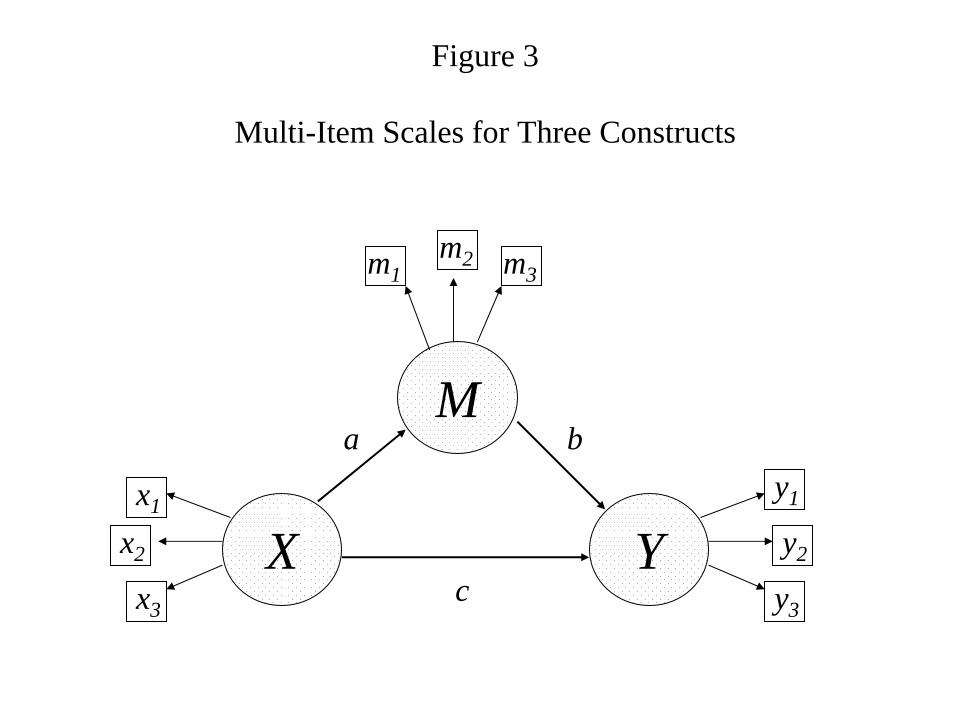
Figure 3

Multi-Item Scales for Three Constructs

X

M

Y

a

c

b

x1

x3

x2

m1

y1

y2

y3

m2 m3

Figure 4

Study 1: Comparing Regression vs. SEM Standard Errors

SE(regr)-SE(sem)

0

0.001

0.002

0.003

0.004

30 50 100 200 500

Figure 5

Study 1: SEM vs. Regression: Sobel z-test of Mediation

Z(sem) - Z(regr)

0.0000

0.0200

0.0400

0.0600

0.0800

0.1000

30 50 100 200 500

100%75%50%25%0% mediation

Figure 6Study 2: The Power of Three Items over One,

for Varying Sample Size

Z(SEM)-Z(reg)

0.0090

0.0190

0.0290

0.0390

0.0490

0.0590

0.0690

30 50 100 200 500

nx=1nx=3

Z(SEM)-Z(reg)

0.0090

0.0190

0.0290

0.0390

0.0490

0.0590

0.0690

30 50 100 200 500

nm=1nm=3

Z(SEM)-Z(reg)

0.0090

0.0190

0.0290

0.0390

0.0490

0.0590

30 50 100 200 500

ny=1ny=3

Figure 7Study 3: Comparing Full SEM to Mean SEM

0

5

10

15

20

25

30

35

No Partial Full

Classification via Full SEM

%C

lass

ified

via

Mea

n SE

M

Correct by Mean SEMIncorrect via Mean SEM

Figure 8Testing Mediation in the Context of a Broader Nomological Network

X

M

Y

A

B C

* *

n.s.

D

E

F

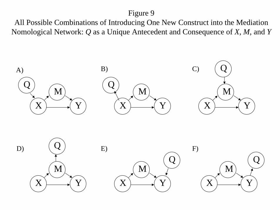
Figure 9All Possible Combinations of Introducing One New Construct into the Mediation

Nomological Network: Q as a Unique Antecedent and Consequence of X, M, and Y

XM

Y

QB) C)A)

Q

XM

Y XM

Y

Q

XM

Y

QD) E) F)

XM

Y

Q

XM

Y

Q

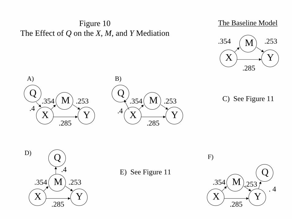
Figure 10The Effect of Q on the X, M, and Y Mediation

XM

Y

The Baseline Model

.354 .253

.285

Q

XM

Y.253

.4

.285

.354

A)

XM

Y

Q

.4

B)

.253

.285

.354 C) See Figure 11

.285X

MY

Q.4

D)

.253.354

XM

Y

Q

. 4

F)

.253

.285

.354E) See Figure 11

Figure 11Do Not Introduce Q as an Antecedent to M or Y

XM

Y

Q.308

.253

.285

.231

C) r’s = 0.4

XM

Y

Q.242

.182

.214

.354

E) r’s = 0.4

XM

Y

Q.887

.253

.285

-.267

C’) r’s = 0.7

XM

Y

Q1.170

-.352

-.319

.354

E’) r’s = 0.7

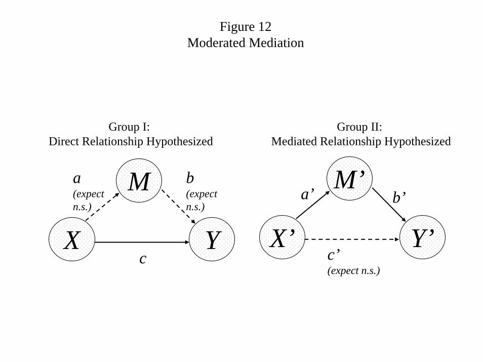
Figure 12Moderated Mediation

Group I: Direct Relationship Hypothesized

Group II: Mediated Relationship Hypothesized

X’

M’

Y’

a’ b’

X

M

Y

a(expect n.s.)

b(expect n.s.)

c’(expect n.s.)

c

Figure 13Mediation Analysis Strategies

2+ Y’s

2+ X’s

#X’s?

#Y’s?

#M’s?

1 or Y

1 or X

1 or M

Structural Equations Models

2+ M’s

Structural Equations Models (or inefficient & biased Regressions)