1

A mathematical representation of the multiaxial Bauschinger effect

C.O. Fredericka and P.J. Armstrong

b

aRail consultant, Derbyshire, UK

E-mail: cofdalbury@sky.com bEmeritus Professor, The Management School. University of Leicester

E-mail: p.armstrong@le.ac.uk

(Reproduction of original 1966 CEGB internal research report in Materials at High

Temperatures Vol. 24, No. 1 pp. 1-26

1. Editorial - R. P. Skelton

Consultant and corresponding author, c/o Science Reviews, PO Box 314, St. Albans,

Herts AL1 4ZG, UK

E-mail: pskelton@scilet.com

The above title and authorship belong to an internal Company Report that was issued

in 1966 [1] and is still often referred to, but it has never been published in the open

literature. The report is reproduced in full below as a paper, but Materials at High

Temperatures has first taken the opportunity to explore the background to what is

regarded by many in the field as a classic work.

1.1 Technical background

The structural integrity of power generating plant components operating at elevated

temperatures depends on the amount of creep and fatigue damage accumulated over

long lifetimes. However, before this material damage can be calculated, the

deformation response of a structure to externally applied loads or constraints must be

assessed. Quite often, the effects of plasticity and creep are allowed for by using

power law equations as an adjustment to initially elastic conditions. This can lead to

pessimistic (i.e., conservative) results and recourse must be made to a fully detailed

inelastic analysis of the structure. For realistic predictions therefore, good

‘constitutive relations’ are required. These should accurately reflect true material

behaviour as when, for example, during start-up and shut-down operations in service,

the location of interest is taken into tension followed by an excursion into

compression. If the material of construction ‘remembers’ its previous history,

subsequent behaviour should be predicted by the equations.

In the study of materials science this history effect had already been given to some

degree by the Bauschinger effect [2]. This may be defined as the lowering of the

absolute value of the elastic limit in compression following a previous tensile loading

and vice versa. Similarly, if deformation in one direction only is considered, loading a

specimen beyond the elastic limit raises the elastic limit for a subsequent load in that

direction. Early interpretations, which are effectively still used today, were couched in

terms of an internal ‘back stress’ which changes sign according to the epoch in the

corresponding stress-strain cycle, which since plasticity is invoked, takes the form of

a hysteresis loop. Masing, a noted investigator, was able to produce a simple model

for the Bauschinger effect during stress reversal [3,4] writing some time later [5] that

“ ... a metal is no mere rigid, dead, body, but is a material that is endowed with

2

something almost like a life of its own, as a result of which many and complex

processes may go on within it.” In other words, a metal may possess a limited

memory of its past history.

For engineering assessment, the mathematical form of the constitutive laws governing

stress-strain behaviour thus depends on (a) the deformation characteristics of the

material, (b) the complexity of the structure and (c) the loading spectrum. There are

many constitutive models, see below, which ideally should take the following into

account:

Non-linear stress-strain response of the material

Material behaviour with repeated cycling (steady-state response, cyclic hardening,

or cyclic softening)

Isotropic hardening (or softening) due to change in yield stress

Kinematic hardening (or softening) due to change in plastic slope

Presence of Bauschinger effect

Relaxation of mean stress under strain control, or strain ratchet under stress

control

Other memory of past deformation

Several constitutive models were reviewed recently [6]. Their properties are very

briefly summarised below. All models [7-13] distinguish between monotonic

(unidirectional) and cyclic behaviour and all take the Bauschinger effect into account.

The list is by no means exhaustive.

Table 1: Capability of various models during cyclic deformation

(after Hales et al., (2002)

Model Loop

curvature

Cyclic

hardening

or

softening

Ratchet Memory

effect

Bi-linear kinematic (ORNL)

[7,8]

No No No* No

As above + plastic work term No Yes No No

As above + memory effect Yes Yes No Yes

Mroz [9] Yes Yes No No

Dafalias [10,11] Yes Yes No No

FRSV [12] Yes Yes No No

Armstrong-Frederick [1] Yes No Yes No

Chaboche (non-linear K + I)

[13]

Yes I or K§ Partial No

As above + memory effect [13] Yes I or K§ Partial Yes

I = Isotropic K = Kinematic

* Allows a change between monotonic and cyclic response § Depending on number and form of linear kinematic terms

3

Models such as those listed above would be used when more simple approaches (e.g.,

a power law) fails to predict a stabilised response for example when a component (a)

experiences only a few large cycles, (b) comprises isolated regions undergoing

plasticity at differing strain ranges or (c) is subjected to a complex loading history [6].

As expected, implementation of many of these models requires a large computational

resource. For the more advanced examples it becomes necessary to describe the

evolution of the stress range (under total strain control) in terms of an appropriate

variable such as the accumulated plastic work (total area of closed hysteresis loops) or

the plastic path length. The latter is defined as the accumulated plastic strain,

independent of sign. Some commercially available finite element codes for structural

analysis make use of some of the above models. Further background descriptions of

constitutive models and their broad classification into ‘Standard’ (decomposition of

total strain into elastic, plastic, creep and anelastic contributions) and ‘Unified’ (creep

and plasticity regarded as arising from the same dislocation source) types can be

found elsewhere [6]. ‘Standard models require a definite yield stress and ‘yield

surface’ and an incremental formulation since FE can distinguish between elastic and

plastic regions. This yield surface can be allowed to expand or contract (isotropic

behaviour) or translate (kinematic behaviour) In principle, distortion of the surface

can also be allowed. Isotropic hardening cannot predict the Bauschinger effect. In

kinematic hardening the degree of translation is a measure of the ‘back stress’. These

are not truly representative of material behaviour but can lead to a high degree of

accuracy.

Amongst the references listed in Table 1 occurs that of Chaboche [13]. This model is

able to capture evolutionary or history-dependent aspects of material response. For

practical use it requires the appropriate hysteresis loop to be described in terms of

several coefficients which are in turn deduced from experimental data. In its simplest

form it employs a kinematic hardening rule to describe a closed hysteresis loop, but

without functions for cumulative plastic strain. The work is a development of the

Armstrong-Frederick model [1] which in turn (as will be seen below) is a

development of the Prager linear kinematic model [7]. Armstrong and Frederick

introduced a ‘recall’ term which influences plastic flow differently for tensile or

compressive loading, depending on the accumulated plastic strain. The model has

become popular and has been incorporated into finite element codes [e.g. 14]. A

feature of the model is a tendency to predict ratchetting under an asymmetrical stress

cycle. This is a result of the operation of the recall term which contains the back

stress.

1.2 Historical setting – structures, specimens, and back stresses

The account given above is a very brief summary of how plasticity theory is currently

conceived and applied in high temperature applications. Thirty to forty years ago

matters were not so clear-cut, and the division between the disciplines of ‘materials

science’ and ‘engineering’ was far sharper than perhaps it is today. The account in

this Section starts in 1977 (strictly, 1975, see below) when Chaboche published a

paper [15] on ‘viscoplastic constitutive equations for the description of cyclic and

anisotropic behaviour of metals’. Computer techniques and capacity had advanced so

that non-linear problems, in this case the deformation response of superalloy IN100

(used in aero-engine turbine blades and discs) at 1000C, could be tackled. A set of

4

constitutive equations, ‘including a hidden internal state parameter’, was employed.

The extra term in the equations accounted for an ‘evanescent strain memory effect’ or

‘delay trace hypothesis’. This was in fact the Bauschinger effect, and the paper

attributed this development to an internal company report by Armstrong and

Frederick [1], issued some eleven years earlier. The analysis was extended to the 3-

dimensional (multiaxial) state. According to the complexity of the model

assumptions, stabilisation of the hysteresis loop could be predicted within a few

cycles, and the results were compared with experiments in load control and strain

control, including periods of stress relaxation.

Further details on the development of the equations are provided below by the authors

themselves. The key point about Chaboche’s (1977) paper [15] is that this was almost

certainly the first time that Armstrong and Frederick’s [1] work had been referred to

in the open literature. The report was produced under the aegis of the erstwhile

Central Electricity Generating Board (CEGB), where publication of unclassified

material was openly encouraged. In the present case this never happened (although an

attempt was made) for reasons given by the authors below. Armstrong and Frederick

were given 10 copies each for distribution amongst their colleagues and the report

was freely available from relevant CEGB libraries. In subsequent publications and

personally, Chaboche himself has always acknowledged his indebtedness to the work.

The report has been cited many times in the open literature (see below) by

investigators who surely cannot have seen the original at first hand. This state of

affairs has arisen because Chaboche’s equations in turn have been incorporated into

finite element and other analytical computer programs [14], see later.

There had in fact been a previous external publication by Frederick and Armstrong

(16). The authors showed that ‘…..if two structures differing only in their initial

internal stresses are subject to the same loading history, the distributions of internal

stress will approach one another in regions of creep and plasticity as the loading

proceeds’. The paper was concerned with engineering structures, for it is not

immediately obvious why such a structure should not ratchet (increase its dimensions

in a given direction) under a repeated load. The paper thus concerned shakedown to a

stable condition, and the authors were able to show that a few cycles of computation

should result in the steady cyclic state, regardless of starting conditions. In fact the

same effect can been demonstrated experimentally in a specimen of stainless steel at

elevated temperatures [17]. Starting from the same (compressive) load in each case,

strain rates were varied randomly over a 2 h period over a fixed total strain range. As

expected, the final stress value was path-dependent. But if any one of those random

strain blocks were regularly repeated at 2 h intervals, it was found that the resulting

hysteresis loop closed within a very few cycles. In terms of what was happening in the

microstructure of the material, it was proposed that hardening (dislocation

accumulation) was opposed by recovery (dislocation annihilation) so that at

corresponding stresses in the random cycle, the to-and-fro motion of dislocations

within the internal (cell) structure were imagined to be identical.

At the time the internal Armstrong-Frederick report [1] was conceived, the editor was

a friend and colleague of Peter Armstrong, although we worked in different

departments at the same CEGB establishment. Regular meetings were held between

‘materials’ (mechanical properties) and ‘engineering’ staff so that we might

5

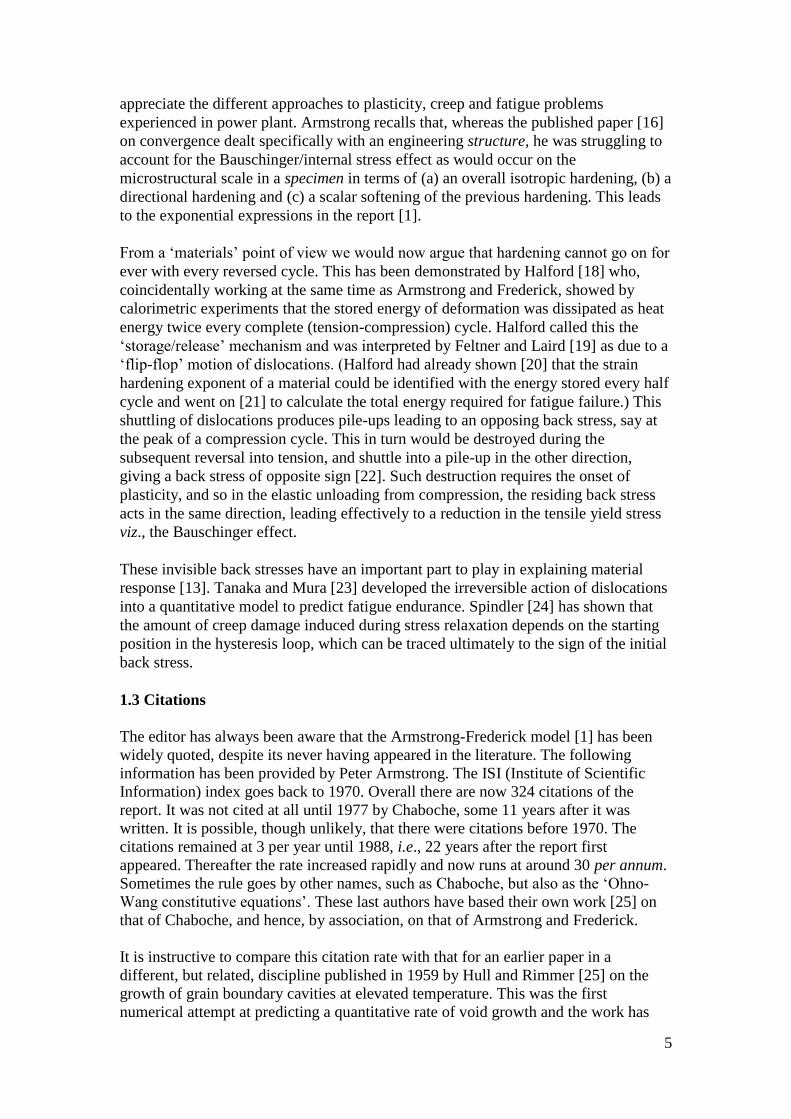
appreciate the different approaches to plasticity, creep and fatigue problems

experienced in power plant. Armstrong recalls that, whereas the published paper [16]

on convergence dealt specifically with an engineering structure, he was struggling to

account for the Bauschinger/internal stress effect as would occur on the

microstructural scale in a specimen in terms of (a) an overall isotropic hardening, (b) a

directional hardening and (c) a scalar softening of the previous hardening. This leads

to the exponential expressions in the report [1].

From a ‘materials’ point of view we would now argue that hardening cannot go on for

ever with every reversed cycle. This has been demonstrated by Halford [18] who,

coincidentally working at the same time as Armstrong and Frederick, showed by

calorimetric experiments that the stored energy of deformation was dissipated as heat

energy twice every complete (tension-compression) cycle. Halford called this the

‘storage/release’ mechanism and was interpreted by Feltner and Laird [19] as due to a

‘flip-flop’ motion of dislocations. (Halford had already shown [20] that the strain

hardening exponent of a material could be identified with the energy stored every half

cycle and went on [21] to calculate the total energy required for fatigue failure.) This

shuttling of dislocations produces pile-ups leading to an opposing back stress, say at

the peak of a compression cycle. This in turn would be destroyed during the

subsequent reversal into tension, and shuttle into a pile-up in the other direction,

giving a back stress of opposite sign [22]. Such destruction requires the onset of

plasticity, and so in the elastic unloading from compression, the residing back stress

acts in the same direction, leading effectively to a reduction in the tensile yield stress

viz., the Bauschinger effect.

These invisible back stresses have an important part to play in explaining material

response [13]. Tanaka and Mura [23] developed the irreversible action of dislocations

into a quantitative model to predict fatigue endurance. Spindler [24] has shown that

the amount of creep damage induced during stress relaxation depends on the starting

position in the hysteresis loop, which can be traced ultimately to the sign of the initial

back stress.

1.3 Citations

The editor has always been aware that the Armstrong-Frederick model [1] has been

widely quoted, despite its never having appeared in the literature. The following

information has been provided by Peter Armstrong. The ISI (Institute of Scientific

Information) index goes back to 1970. Overall there are now 324 citations of the

report. It was not cited at all until 1977 by Chaboche, some 11 years after it was

written. It is possible, though unlikely, that there were citations before 1970. The

citations remained at 3 per year until 1988, i.e., 22 years after the report first

appeared. Thereafter the rate increased rapidly and now runs at around 30 per annum.

Sometimes the rule goes by other names, such as Chaboche, but also as the ‘Ohno-

Wang constitutive equations’. These last authors have based their own work [25] on

that of Chaboche, and hence, by association, on that of Armstrong and Frederick.

It is instructive to compare this citation rate with that for an earlier paper in a

different, but related, discipline published in 1959 by Hull and Rimmer [25] on the

growth of grain boundary cavities at elevated temperature. This was the first

numerical attempt at predicting a quantitative rate of void growth and the work has

6

been referenced almost without fail by materials scientists investigating creep and

creep-fatigue failure mechanisms at elevated temperatures. There have been 504

citations of this publication, currently running at 8 per annum.

It is time that the Armstrong-Frederick seminal work enters the public domain.

Materials at High Temperatures is proud to be able to publish the original, with

permission of British Energy Generation Ltd.

1.4 Comments on the report, and developments since

At the time the report was written, there were few low cycle fatigue (LCF) machines

capable of producing requisite data (see Section 5.2 and elsewhere). From a major

conference twenty two years later [27], LCF tests at high temperature conducted at

total strain range were in proliferation, and continue to this day. Tests at constant

plastic strain range, as referred to in the report, are possible [28, 29] though generally

reserved for specialised studies of material response, such as cyclic deformation under

constant plastic strain rate [30]. Tests at small plastic strain ranges (see Section 5.3. )

are now routine with advanced extensometry, and plastic strain ranges of 10-4

are

achievable [31]. Many elevated temperature multiaxial tests have also been

undertaken since the report [27,32], again continuing to the present time.

In addition to the storage/release energy mechanisms occurring every half cycle (as

discussed in Section 1.2) it is now appreciated that many materials only achieve the

steady state after a period of evolutionary cycling, that is, the hysteresis loop never

completely closes during this stage. Austenitic alloys, for example may harden cycle-

by-cycle while many ferritic alloys soften cycle-by-cycle [6]. These effects, coupled

with ageing phenomena mean that the overall cyclic response of many power plant

alloys changes with service exposure.

Materials scientists and experimentalists generally use the Ramberg-Osgood [33]

power law equation for describing the cyclic strain range as a function of the cyclic

stress range. There are 3 constants (Young’s modulus, a strength coefficient and a

hardening exponent) which uniquely define the stress and strain state, although the

latter two may be allowed to vary in order to describe strain rate effects. It is

distinguished from true constitutive equations in that it is not expressed in incremental

form [6]. However, the equation does not have a definite yield stress, which must

therefore be prescribed as a 0.2% proof stress, 0.1% proof stress etc. It is possible in

principle to identify the Ramberg-Osgood law with the relevant Chaboche equation

[6] but it can be shown that Chaboche constants change with total strain range. It is

also notable that the Ramberg-Osgood law by itself can account for the Bauschinger

effect and accompanying back stress [22].

Turning to the report, there are several instances in the text requiring comment, owing

to the passage of time. The reference to ‘Frederick and Armstrong 1966’ i.e., report

RD/B/N660 refers to one of the internal reports on the assumptions of plasticity

theory discussed by these authors below, and is not the external paper. In the

Discussion Section 8, we read: “The use of the proposed behaviour model for creep

will be the subject of a later report” and also: “It is intended to resolve this question

by incorporating the proposed relationship, the Prager yield criterion and the Von

7

Mises yield criterion as options in a stress analysis computer program.” These

projects were not carried out for reasons explained below by the authors themselves.

As to the comment on the pij parameter, introduced as a microstress and no action

taken to relate it more closely with the actual mechanisms of deformation, the authors

remark: “An attempt to do so by those more qualified than the present authors would

be very useful.” This has been covered to some extent in our Preface.

It is also noteworthy that the authors end their Section 6 (i.e., before their summing

up) with the remark: “…..it would indicate that the proposed behaviour model is on

the right lines.” This has turned out to be something of an understatement.

The report is written in a refreshing and forthright style, salient points being

emphasised by short paragraphs. It is clear from the following recollections that the

authors have not lost this trait. Let the principal players now take up the story.

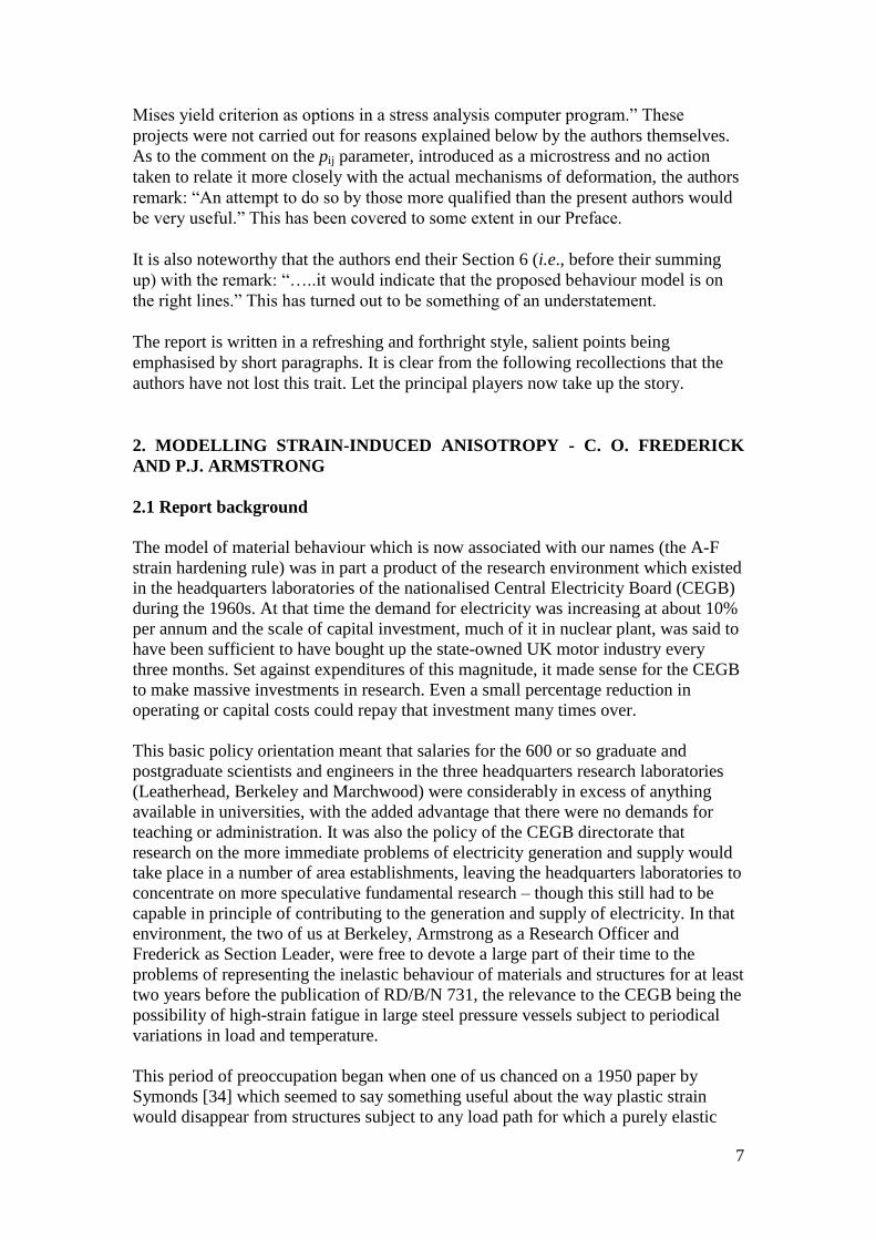
2. MODELLING STRAIN-INDUCED ANISOTROPY - C. O. FREDERICK

AND P.J. ARMSTRONG

2.1 Report background

The model of material behaviour which is now associated with our names (the A-F

strain hardening rule) was in part a product of the research environment which existed

in the headquarters laboratories of the nationalised Central Electricity Board (CEGB)

during the 1960s. At that time the demand for electricity was increasing at about 10%

per annum and the scale of capital investment, much of it in nuclear plant, was said to

have been sufficient to have bought up the state-owned UK motor industry every

three months. Set against expenditures of this magnitude, it made sense for the CEGB

to make massive investments in research. Even a small percentage reduction in

operating or capital costs could repay that investment many times over.

This basic policy orientation meant that salaries for the 600 or so graduate and

postgraduate scientists and engineers in the three headquarters research laboratories

(Leatherhead, Berkeley and Marchwood) were considerably in excess of anything

available in universities, with the added advantage that there were no demands for

teaching or administration. It was also the policy of the CEGB directorate that

research on the more immediate problems of electricity generation and supply would

take place in a number of area establishments, leaving the headquarters laboratories to

concentrate on more speculative fundamental research – though this still had to be

capable in principle of contributing to the generation and supply of electricity. In that

environment, the two of us at Berkeley, Armstrong as a Research Officer and

Frederick as Section Leader, were free to devote a large part of their time to the

problems of representing the inelastic behaviour of materials and structures for at least

two years before the publication of RD/B/N 731, the relevance to the CEGB being the

possibility of high-strain fatigue in large steel pressure vessels subject to periodical

variations in load and temperature.

This period of preoccupation began when one of us chanced on a 1950 paper by

Symonds [34] which seemed to say something useful about the way plastic strain

would disappear from structures subject to any load path for which a purely elastic

8

solution was possible – useful, that is, if we could understand it. The problem was that

neither of us was familiar with the tensor notation in which Symonds’ paper was

written, so we had to figure this out this using clues from the paper itself. In this

respect, the process had something in common with the decipherment of ‘Linear-B’

[35]. Once it had been achieved, a second problem presented itself: that Symonds’

shakedown theorem was based on the highly idealized von Mises yield criterion. This

prompted us to try the substitution of other yield criteria in Symonds’ equations, as a

result of which we made the fortuitous discovery that structures would also shake

down in materials which exhibited Prager kinematic hardening. A paper

demonstrating this was published in the first issue of the Journal of Strain Analysis

[16].

As that paper exemplified, our thinking about the behaviour of structures was

intimately bound up with thinking about the behaviour of materials and both were

bound up with thinking about how to represent structures in computer programmes.

By the mid 1960s computers were becoming capable of handling fairly large arrays

of equations, the question of whether these would be generated by finite difference or

finite element methods was beginning to be resolved in favour of the latter. Either

way, it was clearly important, particularly for the CEGB’s large pressure vessels, that

these equations should represent the inelastic behaviour of the material as accurately

as possible. Reassured about the relevance of what we were doing, and prodded into it

by our Division Head, the late C. H. A. Townley, we produced two internal CEGB

reports which reviewed existing representations of the inelastic behaviour of materials

and attempted to assess their merits, particularly in respect of their representation of

strain-induced anisotropy.

Detailed background of the report

Of particular interest were Batdorf and Budiansky’s ‘slip theory’ [36]which deduced a

yield surface from a simplified model of the behaviour of dislocations and a yield

criterion proposed by Edelman and Drucker [37] which related anisotropy to the total

vector of plastic strain. The problem with the slip theory was that it predicted a yield

surface which would expand in the direction of strain but remain unaltered otherwise,

a prediction clearly inconsistent with any Bauschinger effect. On the positive side, the

physical picture on which it was based, oversimplified though it was, prompted us to

think of the yield surface as displaced by microstresses internal to the material itself,

and thence to the thought that these might shake down in the same way as a structure.

Thoughts along these lines were also encouraged by conversations on the stress-

induced movement of dislocations with the UK editor of this journal with whom

Armstrong travelled to work at the time.

The problem with the Edelman-Drucker yield criterion [37] was that it predicted a

yield surface independent of the path by which the current vector of plastic strain had

been reached. As it stood, this was not even adequate to the case of uniaxial cycling in

tension and compression, since it implied a zero Bauschinger effect. It did suggest,

however, that strain was the crucial variable and that the Bauschinger effect might be

effectively modelled by allowing for a disproportionate effect of more recent strain

We were encouraged in these reflections by references in a paper by Lensky [39] to a

‘principle of delay’ [38] whereby the vector of internal stresses was related to a

specified length of the most recent part of the strain trajectory. Lensky had obtained

9

results consistent with this idea by twisting a thin-walled tube then pulling it, keeping

the twist constant. The resulting decay of torsional stress made it clear that some such

principle of delay did indeed apply to strain-induced anisotropy. The problem with

assuming that the governing parameter was a fixed length of the recent strain

trajectory, however, was that it clearly couldn’t handle cases in which the direction of

strain changed during that fixed length. This pointed towards a relationship between

the increment of strain and the incremental decay of what, by this time we were

calling the ‘strength vector’. At the same time, in order to represent the hardening

effect of the increment of strain, the strength vector had to increase in opposition to it.

Mindful of the 1960s limitations of computing power, the strain hardening rule, as we

proposed it, left it open as to whether or not it was also worthwhile to model any

isotropic strain hardening which might occur. It is striking how concerned we were at

the time to limit both the complexity of the model and the amount of testing required

to determine its parameters.

It wasn’t as easy as this perhaps makes it sound. Armstrong can remember sitting in a

public bar, drawing strain and strength vectors on a beer-mat, to the point that a young

couple introduced themselves as psychologists and enquired if he was suffering from

depression.

There is a certain irony to the fate of RD/B/N 731, the internal CEGB report in which

these ideas were definitively set out [1]. The agreement between Armstrong and

Frederick was that Frederick would take first authorship of the externally published

paper, in recognition of his greater contribution to its mathematical development,

whilst Armstrong would be first author of the internal CEGB report. In the event the

paper was rejected by the journal to which it was submitted, apparently because a

referee ‘could not see the point of it.’ Re-reading the paper after all these years, one

would have thought the point was made very clearly indeed. It is in recognition of the

original agreement, meanwhile, that the paper has been reprinted in this journal with

the names of the authors reversed.

No further attempts were made to publish the paper in an academic journal. It had

been intended to test the A-F rule in a computer programme for analysing the stresses

in thick tubes ‘in order to see whether the computer would come unstuck.’ Since it is

now a well-known weakness of the A-F rule that it predicts ratchetting, this would

probably have sent us back to the drawing-board.

2.2 Subsequent career of C. O. Frederick

Even before the internal publication of the report, however, Frederick had moved to

the Central Electricity Research Laboratories at Leatherhead (CERL) of the CEGB as

head of Structural Engineering Section. Amongst the new problems competing for his

attention were those of analysing stresses in the anchorages of the steel reinforcing

cables of concrete pressure vessels and the automatic generation of finite element

meshes for stress analysis.

When, in November 1965, three out of the eight cooling towers at Ferrybridge C

power station collapsed in winds of only 70 km/h, the detachment of the CEGB’s

Headquarters laboratories from the immediate problems of operation was temporarily

suspended. CERL’s Aerodynamics Section discovered that the design had failed to

10

allow for the Venturi effect created by the proximity of the towers and initiated wind

tunnel experiments to measure mean and dynamic wind pressure values. It was then

the task of Frederick and his team to analyse the consequent vibrational stresses in the

cooling tower shells, using finite elements and modal analysis. Exciting the vibrations

in normal non-windy conditions (to quantify the damping coefficient) was achieved

by swinging against the tower some baulks of timber suspended from a crane. This

worked well but led to a fracas with a local pigeon fancier. When the tower was

struck it acted like a loudspeaker and the noise was sufficient to frighten the pigeons,

preventing their arrival being recorded. Work had to stop for a while!

In 1969, Frederick moved to British Rail as Assistant Director of Research (Track and

Structures, Soil Mechanics and Field Trials Sections (the latter via track experiments

conducted impartial derailment investigations - was the cause due to the track or the

vehicle?). Though most of his time was by now taken up with the management of 80

staff, he still managed to produce papers on such topics as the impact stresses due to

wheel flats and rail buckling. Subsequently, Frederick became responsible for the

Metallurgy and Strength of Materials Sections. Now his earlier experience with stress

analysis and material behaviour became of value.

A problem for which there was no accepted explanation was rail corrugation where

waves (typical wavelength ~ 50mm and depth ~ 0.1mm) form on the ‘running table’

of the rail. The effect of these waves is (a) to create enhanced and environmentally

unacceptable noise and (b) to greatly increase the pressure of wheel-rail contact,

causing cracks to form near the rail surface. It is customary to grind the rails to

remove the waves. Unfortunately, the waves may rapidly return and often the grinding

fails to remove the cracks. These cracks grow deeper until they can bring about rail

fracture. A research contract showed that the corrugation problem was one of periodic

wear of the running table of the rail. In this process, a small wave can deepen

progressively. After several years of running the project Frederick wrote a chapter on

rail corrugation for a book on permanent way. He later realised that the process

depended on periodic creep (relative movement between wheel and rail) having the

right phase with respect to a very shallow pre-existing wave. But how could you

calculate the phase?

In between times, the differential equations governing the interaction of wheels and

track still found ways of intruding on his leisure. During a fishing holiday, he realised

that an instability in these equations might account for the differential wear which

causes corrugations of rails. In 1986 he published “A Rail Corrugation Theory” and

presented at a conference on Contact Mechanics and Wear in Rhode Island USA.

Though an entirely reliable prediction of this effect remains elusive, this has been

acknowledged as something of a breakthrough.

Rather less tenable was Frederick’s interest in the notion of a propulsion system using

laser-induced fusion pulsed at high frequency. Having failed to get his ideas published

(once more!), this time in the journal Spaceflight, Frederick took out a provisional

patent on the concept whilst its feasibility was explored. Eighteen months are allowed

for this process. In the patent assessment it had to be demonstrated in a practical

situation. Hence it was shown as part of a flying saucer. When the deadline arrived it

was realised that there would be no commercial benefit in a patent but publication

would make the principle freely available. Several papers meanwhile had given

11

encouraging reports on progress with laser fusion. It was decided to proceed with the

patent for 1 year in the UK. So it came about that British Rail published a patent [40]

for a flying saucer powered by laser-induced fusion.

Though Frederick retired in 1994, he has been in demand as a consultant especially on

rail matters and was called upon to give evidence at the Railtrack inquiry into the

Hatfield Crash (which was caused by a broken rail).

2.3 Subsequent career of P. J. Armstrong

In 1967, the year following the publication of RD/B/N 731, Armstrong left

engineering altogether, probably influenced, it is now embarrassing to relate, by the

low opinion of engineering held by the literary persons with whom he associated at

that time. After an MSc in the Sociology of Science and Technology, he worked as a

research assistant on a study of shop-floor industrial relations. The low point of his

career was five years of teaching general studies at a small and eccentrically-run

college of further education. Managing to scramble back into academic life with

another research assistantship at the age of 39 he eventually produced a study which

explained the low status of engineering in the UK in terms of the ascendancy of

accountants. Simple as it seems, that study and the work which flowed from it,

established his reputation as a social scientist and led, ironically, to a chair in

accounting at the University of Sheffield. Altogether he has published four books and

35 refereed journal articles in the field of social science, some of which are quite well

known in their particular areas, but none of them has been as consequential as the

unpublished CEGB report of forty years ago. Now aged 67, he is once again enjoying

the freedom to pursue his research, this time as a part-time Consultant Professor at the

University of Leicester.

2.4 Developments to date

Unknown to both Frederick and Armstrong, RD/B/N 731 and the A-F strain

hardening rule went on to enjoy lives of their own. Armstrong discovered the

continuing relevance of RD/B/N731 by accident a few years ago whilst searching the

citation indices for other purposes. The discovery prompted him to get in touch with

Frederick and to mention the matter to the European editor of this journal, who was

also a colleague at CEGB Berkeley at the time and with whom he had remained in

contact over the years. (He also suggested that Prof. J.-L. Chaboche be contacted to

obtain his side of the story.) This account of our work at CEGB in the 1960s is a

product of that accident.

3. MY SIDE OF THE STORY – J. L. CHABOCHE

ONERA, DMSE/LCME, BP 72, 29 Av. de la Division Leclerc, 92322, Chatillon,

Cedex, France.

E-mailJean-Louis, Chaboche@onera.fr

3.1 Discovering the A-F Report

12

At the beginning of the seventies, at ONERA, in the Laboratory of Jean Lemaître, we

were mainly working around viscoplastic constitutive equations based on isotropic

hardening, performing many different structure-like high temperature tests with

complex multiaxial loads, but essentially under monotonic or quasi-repeated

conditions. When the first hydraulic fatigue machine for tension-compression testing

arrived, we literally re-discovered the importance of Bauschinger effects and the non-

isotropic nature of hardening (in transient conditions, as well as in creep). After some

tentative steps to define updating rules, we were obliged to accept the notion of an

evolving back stress (although not called as such), a concept not so well known (at

least by us) at that time, because we were more involved in the field of creep rather

than in plasticity.

If I remember well, I was trying several approaches following an article by Malinin

and Khadjinsky [41] in the context of creep, that combined a hardening and a static

recovery term for the evolution equation of the so-called additional stress. The paper

also referred to the work by Ilyushin [39] and the “delay trace hypothesis. At that

time, probably in the spring 1974, I independently discovered the basic Armstrong-

Frederick rule, incorporating in the simplest way the fundamental hardening/dynamic

recovery format for the additional stress. When doing so, writing this equation in its

3D form for the first time, and discovering its easy closed form integration for

uniaxial tension-compression conditions, I recall that I was working on my hands and

knees on the living-room carpet, and I was very happy with the result……

I do not remember exactly how I came to know about the existence of the Armstrong-

Frederick CEGB Report. Until very recently, before the editor asked me to take part

in this Preface, I was under the impression that I read the reference in the Malinin &

Khadjinsky [41] paper. In fact, it is not, as checked recently. How I obtained it is a

mystery to me now. (May be a reader could help?) Anyway, I asked the ONERA

library to try to obtain this A-F report. At that time it was not too difficult; I obtained

the Report a few weeks later, and discovered “my” equation in it, with many other

good things, published about 8 years before.

I presented my “viscoplastic constitutive equation”, mainly based on the A-F rule

(applied in the context of unified viscoplasticity, with some modifications and

additions, together with some very good simulations on IN100 nickel base superalloy)

at the XVIIth Polish Solid Mechanics Conference which took place in Szczyrk in July

or August 1975. At this conference, just after my lecture, I was asked by Antoni

Sawczuk (who shortly became President of the Polish Academy of Sciences) to

publish an extended version in the Bulletin de l’Académie Polonaise des Sciences. I

was very happy to do so, and the paper appeared in 1977 [15].

This paper seems to be one of the first to reference the unpublished Armstrong and

Frederick Report [1]. In my subsequent papers in this domain, I have always indicated

this Report as the formative work, and I am gratified now to realize over the past few

years, that I have unwittingly contributed to the recognition of this work and to the

fact that the ‘Armstrong-Frederick rule’ now appears to have entered the general

vocabulary.

13

3.2 Subsequent developments and career

After this initial investigation, with my 1977 paper [15] and my PhD thesis

completed, I continued working and publishing along these lines, introducing several

developments, couplings with isotropic hardening, including multiple back-stresses

obeying the A-F rule, adding some “strain range memory” effects etc. etc. Many other

unified cyclic viscoplastic theories were also under development in the same period,

using similar concepts, attempting to reconcile cyclic plasticity and creep flow (e.g.,

refs [42-46]. One advantage of my own approach, mainly based on the very simple

structure of the A-F rule, was that it was simple to integrate in closed form (for

proportional cyclic conditions) and easily incorporated in a more fundamental

thermodynamic framework.

Though involved in many other contexts such as Continuum Thermodynamics, Finite

Element (FE) Analyses, Computational schemes, Continuum Damage Mechanics,

Fracture Mechanics, Multiscale Analysis etc., my whole career has remained with

research in Solid Mechanics but from time to time going back to my initial interests in

cyclic plasticity and viscoplasticity. I have been publishing papers with some

comparisons [47, 48] between various different plasticity and viscoplasticity theories,

showing similarities and differences, discussing drawbacks and advantages, again

acknowledging the contribution of this unpublished but renowned Armstrong-

Frederick Report [1].

3.3 Ratchetting conditions, presently applied equations and FE codes

One of the difficulties associated with the A-F rule is the fact that it predicts too much

ratchetting under non-symmetric loading conditions. At the end of the eighties, it was

decided to develop an improved rule, using a threshold in the dynamic recovery term

[49, 50]. Such a solution has subsequently served other researchers, e.g Ref [25]. It

seems that other modifications, developments, improvements, which have taken place

all defer to the A-F Report as containing the “reference rule”. It is surprising to

observe that this reference “A-F model” is most often taken in order to mention its

main defect, its poor capabilities under ratchetting conditions, so justifying some

better (but more complicated) modification.

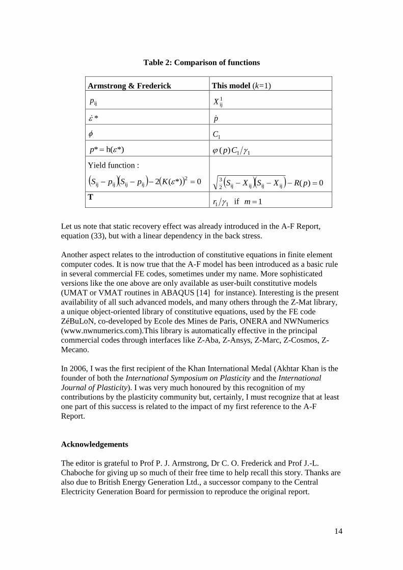
In order to illustrate the above-mentioned complications of the presently applied

models compared to the initial version by Armstrong & Frederick [1], referring to

equation (33), I am happy to write the set of equations:

(k)ijij XX

(k)ij

1(k)

k(k)

(k)ijk(k)

kpijkij )()(

3

2XXprp

X

XCXpCX

m

k

with the following correspondence between variables and material parameters set out

in Table 2. Identification is possible with only one back stress (k = 1), 0 and m =

1 in the above recent version :

14

Table 2: Comparison of functions

Armstrong & Frederick This model (k=1)

ijp 1ijX

* p

1C

*)h(* p 11)( Cp

Yield function :

0*)(22

ijijijij KpSpS

0)(ijijijij2

3 pRXSXS

T 11 r if 1m

Let us note that static recovery effect was already introduced in the A-F Report,

equation (33), but with a linear dependency in the back stress.

Another aspect relates to the introduction of constitutive equations in finite element

computer codes. It is now true that the A-F model has been introduced as a basic rule

in several commercial FE codes, sometimes under my name. More sophisticated

versions like the one above are only available as user-built constitutive models

(UMAT or VMAT routines in ABAQUS [14] for instance). Interesting is the present

availability of all such advanced models, and many others through the Z-Mat library,

a unique object-oriented library of constitutive equations, used by the FE code

ZéBuLoN, co-developed by Ecole des Mines de Paris, ONERA and NWNumerics

(www.nwnumerics.com).This library is automatically effective in the principal

commercial codes through interfaces like Z-Aba, Z-Ansys, Z-Marc, Z-Cosmos, Z-

Mecano.

In 2006, I was the first recipient of the Khan International Medal (Akhtar Khan is the

founder of both the International Symposium on Plasticity and the International

Journal of Plasticity). I was very much honoured by this recognition of my

contributions by the plasticity community but, certainly, I must recognize that at least

one part of this success is related to the impact of my first reference to the A-F

Report.

Acknowledgements

The editor is grateful to Prof P. J. Armstrong, Dr C. O. Frederick and Prof J.-L.

Chaboche for giving up so much of their free time to help recall this story. Thanks are

also due to British Energy Generation Ltd., a successor company to the Central

Electricity Generation Board for permission to reproduce the original report.

15

Editor’s note on the text

The original report has been scanned and the type reset exactly as in the original, but

using the numerical system of references as in the style of Materials at High

Temperatures. However, where possible, investigators names have been retained in

the text so as not to alter the sentence structure. Obvious minor spelling mistakes have

been corrected. The Figures similarly are scanned in from the originals, and so reflect

the style of the mid 1960’s and the units in use at the time.

References to preface

[1] Armstrong, P.J. and Frederick, C.O., A mathematical representation of the

multiaxial Bauschinger effect, CEGB Report RD/B/N731. (1966).

[2] Bauschinger, J., On the changes of the elastic limit and the strength of iron and

steel by straining in tension and compression, by heating and by cooling and by

frequently repeated loading, Mitt Mech, Tech. Lab. Munchen, 13, 1-115. (1886).

[3] Masing, G. On Heyne’s hardening theory of metals due to inner elastic stresses (in

German) Wiss Veröff Siemens-Konzern, 3, 231-239 (1923)

[4] Masing, G. Eigenspannungen un Verfestigung beim Messing in Proc. 2nd

int.

Congr. Applied Mechanics. Zürich, Switzerland, pp. 332-335 (1926)

[5] Masing, G. The Foundations of Metallography. Monograph and Report Series No.

21, The Institute of Metals, London p.16 (1956)

[6] Hales, R., Holdsworth, S. R., O’Donnell, M. P., Perrin, I. J. and Skelton, R. P., A

Code of Practice for the determination of cyclic stress-strain data, Mater. High Temp.,

19, 165-185. (2002)

[7] Prager, W., The theory of plasticity: A survey of recent achievements, Proc.

I.Mech.E., 169, 21, 41-57. (1955).

[8] Pugh, C.E. Clinard, J. A. and Swinderman, R. W., Currently recommended

constitutive equations for inelastic design analysis of FFTE components, ORNL-TM-

3602. (1971).

[9] Mroz, Z., On the description of anisotropic work hardening, J. Mech. Phys. Solids,

15, 165-175. (1976).

[10] Dafalias, Y.F., Modelling cyclic plasticity: Simplicity versus sophistication, in

Mechanics of Engineering Materials, C S Desai and R H Gallagher (Eds), John

Wiley, 153-178. (1984).

[11] Khan, A.S. and Huang, S., Continuum Theory of Plasticity, Wiley Inter-Science.

(1995).

[12] White, P.S., Hübel, H., Wordsworth, J. and Turbat, A., Guidance for the choice

and use of constitutive equations in fast reactor analysis, Report of CEC Contract

RA1-0164-UK. (1993).

[13] LeMaître, J. and Chaboche, J.-L., Mechanics of Solid Materials, Cambridge

University Press, (1990).

[14] ABAQUS, Version 6.6, ABAQUS UK Ltd. Birchwood, Warrington, UK

[15] Chaboche, J.L. Viscoplastic constitutive equations for the description of cyclic

and anisotropic behaviour of metals. in XVIIth

Polish Solid Mechanics Conf. Szezyrk,

subsequently published in Bull. de L’Academie Polonaise des Sciences, Série Sciences

et Techniques, 1977 Vol. 25, pp. 33-41 (1975)

16

[16] Frederick, C.O. and Armstrong, P.J. Convergent internal stresses and steady

cyclic states of stress. The Journal of Strain Analysis. Vol. 1, No. 2. pp. 154-159.

(1966).

[17] Skelton, R. P., Stress relaxation during high temperature high strain fatigue,

Mater. Sci. Eng., 22, 213-222. (1976).

[18] Halford, G. R., Stored energy of cold work changes induced by cyclic

deformation, PhD thesis, University of Illinois. (1966).

[19] Feltner, C. E. and Laird, C., 1967, Cyclic stress-strain response of FCC metal and

alloys – II: Dislocation structures and mechanisms, Acta Metall., 15, 1633-1653.

[20] Halford, G. R. The strain hardening exponent – a new interpretation and

definition. Trans. ASME 56, 787-788 (1963).

[21] Halford, G. R., The energy required for fatigue, J. Mater., 1, 1-38. (1966).

[22] Skelton, R.P., Bauschinger and yield effects during cyclic loading of high

temperature alloys at 550°C, Mater. Sci. Technol., 10, 627-639. (1994)

[23] Tanaka, K. and Mura, T., A dislocation model for fatigue crack initiation, J.

Appl. Mech., 48, 97-103. (1981)

[24] Spindler, M. W., The prediction of creep damage in type 347 weld metal, Part I:

The determination of material properties from creep and tensile tests: Part II: Creep-

fatigue tests, Int. J. Pressure Vessels and Piping, 82, 175-194. (2005).

[25] Ohno, N. and J.D. Wang, Kinematic hardening rules with critical state of

dynamic recovery, Parts I and II, Int. J. of Plasticity, 9, pp. 375-403. (1993).

[26] Hull, D. and Rimmer, D. E., The growth of grain boundary cavity voids under

stress, Phil. Mag., 4, 673-687. (1959).

[27] Solomon, H. D. et al. (eds.) Low Cycle Fatigue, ASTM STP 942, Amer. Soc.

Testing Mater., Philadelphia. (1988).

[28] Wilson, C. J., and Robinson, A., Control of plastic extension in fatigue tests, J.

Phys. E: Sci. Instr., 10, 129-132. (1977).

[29] Christ, H.-J., Mughrabi, H., Petry, F. Zauter, R. and Eckert, K., The use of

plastic strain control in thermo-mechanical fatigue testing, in: Fatigue under Thermal

and Mechanical Loading, Kluwer Academic Publishers, Dordrecht, pp. 1-14. (1996).

[30] Maier, H. J. and Christ, H.-J., Modelling of cyclic stress-strain behaviour and

damage mechanisms under thermo-mechanical fatigue conditions, Int. J. Fatigue, 19,

pp. S267-S274. (1998).

[31] Lukáš, P. and Klesnil, M., Cyclic stress-strain response and fatigue life of metals

in low amplitude region, Mater. Sci. Eng., 11, 345-356. (1973).

[32] Ohnami, M., Plasticity and High Temperature Strength of Materials – Combined

Micro- and Macro-Mechanical Approaches, Elsevier Applied Science, London.

(1988).

[33] Ramberg, W. and Osgood, W.R., Description of stress-strain curves by three

parameters, NACA Tech Note No. 902. (1943).

[34] Symonds, P.S. Shakedown in Continuous Media. Trans. A.S.M.E. Paper No. 50-

A-17 (1950).

[35] Ventris, M. and Chadwick, J., Documents in Mycenean Greek, Cambridge

University press, London. (1956).

[36] Batdorf, S.B. and Budiansky, B. Theory of plasticity based on the concept of slip.

N.A.C.A. Technical Note 1871. (1949).

[37] Edelman, F. and Drucker, D.C. Some extensions of elementary plasticity theory.

Journal of the Franklin Institute Vol. 251 pp. 581-605, (1951).

17

[38] Lensky, V.S. Analysis of Plastic behaviour of Metals under Complex Loading. in

Lee, E.H. and Symonds, P.S. Plasticity. London. Pergamon Press. (1960).

[39] Ilyushin, A.A. On the relation between stress and small deformation in the

mechanics of continuous media. Prikl Mat. Mekh, Vol. 18, No. 6, pp. 641-666.

(1954).

[40] UK Patent No. GB1310990. The Patent Office. London.

[42] Bodner, S.R., Partom, Y., Constitutive Equations for Elastic Viscoplastic Strain-

Hardening Materials, Trans. ASME, J. of Appl. Mechanics, 42, pp.385-389. (1975)

[43] Miller, A., An Inelastic Constitutive model for Monotonic Cyclic and Creep

Deformation, J. of Engng Materials and Technology, J. Engng Materials and

Technology, 98, 2, pp.97-105 and 106-113. (1976).

[44] Robinson, D.N., A unified creep-plasticity model for structural metals at high

temperature, Oak Ridge Laboratories Report. ORNL, TM-5969. (1978).

[45] Walker, K.P., Research and Development Program for Non-Linear structural

Modeling with Advances Time-Temperature Dependent Constitutive Relationships,

Report PWA-5700-50, NASA CR-165533. (1981).

[46] Krempl, E., McMahon, J.J., Yao, D., Viscoplasticity based on overstress with a

differential growth law for the equilibrium stress, 2nd

Symp. on Non-Linear

Constitutive Relations for High Temperature Applications, NASA, Cleveland, Ohio,

(1984) Publ. Also published in Mechanics of Materials, 5, pp. 35-48, (1986)

[47] Chaboche, J.L., Time independent constitutive theories for cyclic plasticity, Int.

J. of Plasticity, 2, no.2, pp.149-188 (1986).

[48] Chaboche, J.L., Constitutive equations for cyclic plasticity and cyclic

viscoplasticity, Int. J. of Plasticity, 5, No. 3, pp.247-302. (1989).

[49] Chaboche, J.L., On some modifications of kinematic hardening to improve the

description of ratchetting effects, Int. J. of Plasticity, 7, No.7, pp.661-678, (1991).

[50] Chaboche, J.L., Nouailhas, D., Pacou, D., Paulmier, P., Modeling of the cyclic

response and ratchetting effects on inconel-718 alloy, European J. of Mechanics, 10,

No.1, 1991, pp.101-121. (1991).

18

REPRODUCTION OF THE ORIGINAL REPORT

RD/B/N731

Central Electricity Generating Board

Research & Development Department

A Mathematical Representation of the Multiaxial Bauschinger Effect

By P. J. Armstrong and C. O. Frederick

Berkeley Nuclear Laboratories

December 1966

19

SUMMARY

Inelastic stress analysis would be totally impractical without simplified mathematical

models of the behaviour of structural materials. Naturally these should be as accurate

as possible; they should, for instance, display a Bauschinger effect in time-

independent plasticity.

Existing attempts to do this do not appear to be wholly adequate and a new material

behaviour model is proposed here. On the available evidence it appears to represent

plasticity more accurately than previous models.

The extension of the proposed behaviour model to include time dependent effects is

discussed briefly.

1. INTRODUCTION

In the interests of economy, it is necessary to reduce the sections employed in a

structure as far as safety considerations will allow. Reduced sections imply higher

stresses and, in many structures, e.g. pressure vessels, a certain amount of inelastic

strain is tolerated. The current design codes for such structures are based on a

combination of service experience, experimental data and approximate theory. Further

design advances, that is, a further reduction in sections, can only be achieved without

reducing safety margins if stresses and strains are known more accurately. It is true

that component testing plays an indispensible part in this process, but the data

obtained can only be extrapolated to untested geometries if theoretical analyses are

available. For this reason, it is likely that inelastic stress analysis, using computer

programs to deal with the complex geometries encountered in practice, will play a

vital part in formulating the design codes of the future.

Any such computer program must incorporate some assumptions about the behaviour

of the material. At the outset the problem is simplified by treating the material as a

continuum although it will, in fact, have a granular structure. The actual behaviour of

an element of this continuum depends on the stress system acting on it, the

temperature to which it is subjected and its previous strain-temperature history. It is

plainly impossible to obtain data appropriate to all the conditions likely to arise in a

structure. Furthermore, if such data were available, it would be a gigantic task to feed

it into a computer, even supposing the storage capacity were adequate.

The complexity of inelastic behaviour makes the use of approximate mathematical

models essential. It is usual to assume that inelastic strains can be separated into time-

dependent creep strains and instantaneous plastic strains. In reality, all inelastic strain

is time-dependent (Marsh and Campbell 1963) and could, in theory, be treated as

creep. In practice the strain rates are sometimes very high and the computer program

would have to re-calculate the stress distribution in the structure at very small

intervals of time. It is more convenient to treat inelastic strain occurring at large strain

rates as if it were instantaneous. In other words, the separation of creep and plastic

strain is justified on practical grounds. This is discussed more fully by Frederick and

Armstrong (1966).

20

Most existing computer programs for inelastic stress analysis assume that plastic

strain takes place according to elastic-perfectly plastic theory when the stresses satisfy

the Von Mises yield criterion. For steady-state creep, the corresponding assumption is

that there is a power-law dependence of the equivalent creep strain rate on the

equivalent stress. It is important to remember that these and all such mathematical

models of material behaviour are approximate.

One of the factors ignored by elastic-perfectly plastic theory is the well known fact

that tensile plastic strain increases the tensile yield stress of a metal above the

compressive yield stress. This is a particular case of the Bauschinger effect. Similar

effects exist under multiaxial stress conditions and there are analogous effects in

creep. Creep recovery is the best-known instance of the latter.

If material behaviour laws which neglect these factors are used in stress analysis, the

results must be in error. The extent of this error is virtually impossible to estimate.

Therefore, in order to increase confidence in the results of stress analysis computer

programs, more accurate models of inelastic material behaviour must be found. At the

same time, these models must remain fairly simple and the data necessary to fit the

models to a particular material must be readily obtainable.

The behaviour model presented here is based on the concept of internal microstress. It

is concerned mainly with time-independent plasticity though a method of extending it

to cover time-dependent creep is also introduced. In particular, it is a more realistic re-

presentation of the multiaxial Bauschinger effect than any of the models hitherto

proposed. The predictions of the proposed model are compared with experimental

data published by Lensky (1960), Benham (1961) and Wood (1956).

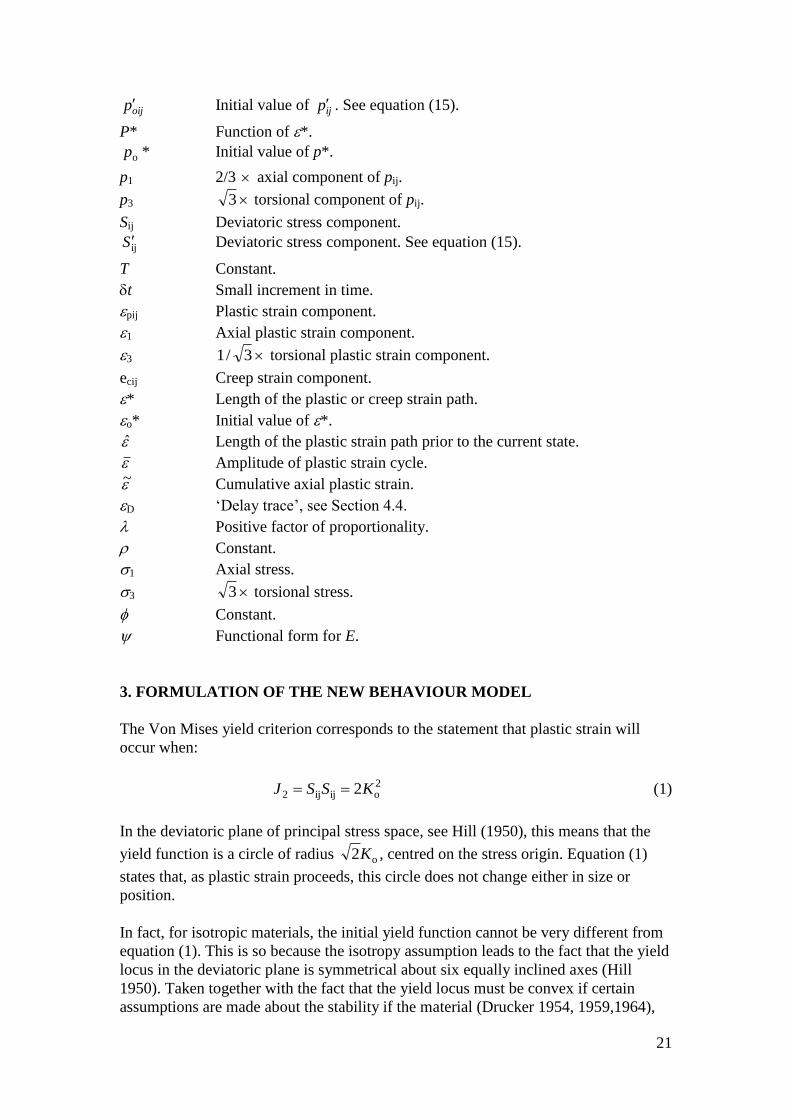
2. NOTATION

E Energy dissipation rate in the microstructure.

f(*) Function defining the variation of K with *.

*ij g Function defining the variation of pij with.

*ij g Differential of gij with respect to *.

Gij Constant value of ijg for a straight plastic strain path.

h(*) Function defining the variation of p* with *

i, j Suffices taking the values 1, 2 or 3.

J2, J3 Second and third invariants of the deviatoric stress respectively.

K Yield stress in shear.

Ko Initial yield stress in shear.

k, l Suffices similar to i, j. See equation (32).

n Number of half strain cycles.

pij ‘Microstress’ component.

ijp ‘Microstress’ component. See equation (15).

poij Initial value of pij.

21

oijp Initial value of ijp . See equation (15).

P* Function of *.

*op Initial value of p*.

p1 2/3 axial component of pij.

p3 3 torsional component of pij.

Sij Deviatoric stress component.

ijS Deviatoric stress component. See equation (15).

T Constant.

t Small increment in time.

pij Plastic strain component.

1 Axial plastic strain component.

3 3/1 torsional plastic strain component.

ecij Creep strain component.

* Length of the plastic or creep strain path.

o* Initial value of *.

Length of the plastic strain path prior to the current state.

Amplitude of plastic strain cycle.

~ Cumulative axial plastic strain.

D ‘Delay trace’, see Section 4.4.

Positive factor of proportionality.

Constant.

1 Axial stress.

3 3 torsional stress.

Constant.

Functional form for E.

3. FORMULATION OF THE NEW BEHAVIOUR MODEL

The Von Mises yield criterion corresponds to the statement that plastic strain will

occur when:

2oijij2 2KSSJ (1)

In the deviatoric plane of principal stress space, see Hill (1950), this means that the

yield function is a circle of radius o2K , centred on the stress origin. Equation (1)

states that, as plastic strain proceeds, this circle does not change either in size or

position.

In fact, for isotropic materials, the initial yield function cannot be very different from

equation (1). This is so because the isotropy assumption leads to the fact that the yield

locus in the deviatoric plane is symmetrical about six equally inclined axes (Hill

1950). Taken together with the fact that the yield locus must be convex if certain

assumptions are made about the stability if the material (Drucker 1954, 1959,1964),

22

the influence of J3 on the yield function must be small. This is confirmed by

experiment (Hill 1950, Ford and Alexander 1963).

If the material remains isotropic as plastic strain proceeds, equation (1) can only be

modified by the substitution of K for Ko. In the deviatoric plane of principal stress

space, this means that the yield circle changes in size but remains centred on the stress

origin.

Experiments have shown however, that materials do not, in general, remain isotropic

when plastically strained (Naghdi, Essenburg and Koff 1957, Ivey 1961, Pugh, Mair

and Rapier 1962, for example). These tests show that the yield locus changes in shape

and position as well as size.

In considering the work-hardening properties of isotropic materials, Hill (1950)

suggested that the size of the yield locus could be assumed to be a function either of

the plastic work or of the length of the plastic strain path. There is probably little to

choose between the two and it is convenient to make the second assumption here (see

equation (8)).

The changes in shape of the yield locus during plastic strain are complex and no clear-

cut picture has so far emerged from experimental data. For example, it is still a matter

of controversy whether “corners” can be induced on the yield surface or not (Mair

1966). For this reason, the behaviour model presented here makes no allowance for

possible changes in shape of the yield locus.

It has been known for many years that the yield locus changes its position during

plastic strain. In uniaxial tests, it is well known that tensile plastic strain raises the

tensile yield stress above the compressive yield stress. This is the Bauschinger effect

and it is a particular case of the changes in position of the yield locus reported by the

workers referred to above.

Edelman and Drucker (1951) presented several yield functions which incorporate a

simulation of the Bauschinger effect. One of these is equivalent to a postulate due to

Prager (1956) and may be written:

2opijijpijij 2KSS (2)

Comparing this with equation (1), it can be seen that, in the deviatoric plane of

principal stress space, the yield locus is still a circle radius o2K . The centre of the

circle, however, is now displaced by a vector proportional to the plastic strain vector.

This means that deformation in a certain direction increases the resistance of the

material to further deformation in that direction. Although equation (2) has its

shortcomings, this idea is plausible both on mechanical and metallurgical grounds and

it will be used in what follows.

In the uniaxial case, equation (2) results in a linear strain hardening curve and the

compressive yield stress is reduced during tensile plastic strain by an amount equal to

23

the increase in tensile yield stress. Equation (2), therefore, is a step forward in the

attempt to simulate the Bauschinger effect. Clearly, equation (2) could be made more

general by introducing K in place of Ko where K as before, is a function of the length

of the plastic strain path.

Equation (2) and the other yield functions introduced by Edelman and Drucker (op.

cit.) have one important feature in common. This is that the sole factor determining

strain-induced anisotropy, i.e. the displacement of the yield locus, is the current

plastic strain. This means that the plastic strain path by which the current plastic strain

was reached, does not influence the current behaviour of the material, except, perhaps,

to modify the size of the yield locus. If the size of the yield locus is assumed to

depend only on the length of the plastic strain path, different strain paths of equal

length, if they result in the same total plastic strain, will result in identical material

behaviour.

Fig. 1 Two plastic strain paths to give same net plastic strain

One implication of this is shown in Fig. 1. O represents the strain origin and OP, the

plastic strain vector. P can reach strain point B by either of two semicircular strain

paths, OAB and OCB. Suppose, on reaching B, the strain vector tip, P, moves along

the line BD, tangential to circle OABC. If point P has followed path OCBD, the strain

direction is unaltered at B. On the other hand, if point P has followed the route

OABD, the direction of plastic strain is reversed at B. If strain-induced anisotropy is

assumed to depend only on the current plastic strain, the resistance to straining along

line BD should be the same in the two cases. This scarcely seems plausible. The yield

locus at B must depend in some way on internal microstresses. These can scarcely be

the same when such different plastic strain paths have been followed.

24

This leads naturally to the representation of the internal microstress by a stress -pij.

The net stress causing plastic strain in the microstructure is then Sij - pij. The yield

function corresponding to equation (1) is:

2oijijijij 2KpSpS (3)

The displacement of the yield locus is then governed by pij. As with equations (1) and

(2), changes in size of the yield locus can be allowed for by replacing Ko in equation

(3) by K, where K is a function of the length of the plastic strain path. It then remains

to find a plausible relationship between pij and the plastic strain path.

Ilyushin (1954) postulated that the material behaviour relationships at a point depend

not on the whole of the previous strain path but only on a certain length of the most

recent part of it. The postulate was concerned with total strain paths but, on physical

grounds, it is plausible that similar considerations apply to plastic strain paths.

Suppose that the length of the prior strain path which influences current conditions is

D (the “delay-trace”) and that strain point P removes away from strain point X as

shown in Fig. 2. When the distance between P and X is equal to or greater than D, the

only prior strain history the material “sees” is the straight strain path XP. The stress

vector at P is then colinear with the strain path. During portion XP of the strain path,

the stress vector tends to become colinear with the strain path as in Fig. 2. For total

strain paths, this effect has been demonstrated by Lensky (1960).

In other words the delay trace hypothesis asserts that the material behaviour

relationships at P will be influenced by conditions at X until the arc-length between

them is D. The influence of conditions at X has then disappeared. Two criticisms can

be raised at the delay trace hypothesis in this form.

Firstly, its use in computer programs would mean that conditions over a certain length

of the strain path would have to be “remembered” by the computer. Secondly it does

not seem physically plausible that referring to Fig. 2, conditions at X will ever entirely

cease to influence conditions at P. It is more likely that the influence of conditions at

X diminishes asymptotically to zero as the arc length between points P and X

increases. Using the idea behind Ilyushin’s postulate and the Prager yield criterion

together with the microstress concept, a hypothesis can be formulated which meets

these objections.

Consider a material in an initial state represented by poij which is then subjected to an

increment in plastic strain tδpij . It will be assumed that the plastic strain affects the

material in two ways. Firstly, the resistance to further strain in the direction of the

plastic strain increment increases. This can be simulated by adding to poij an

increment in pij proportional to pijt. Secondly, the plastic strain increment

diminishes the effect of poij on conditions after the plastic strain increment has taken

place. This can be simulated by reducing the components of poij by an amount

proportional to their initial value and the arc length of the plastic strain increment. In

other words, poij is decreased by an amount proportional to tp δ*oij . These two

effects may be written:

25

*

*

ij

pijij p

pp (4)

where p* is some scalar function of the plastic strain path. As with K, it appears

reasonable to regard p* as a function of the arc length of the plastic strain path.

Fig. 2 Illustration of “Delay Trace” hypothesis

This hypothesis has the advantage that, in order to take account of the previous strain

path, a computer program need only “remember” the value of pij. Furthermore, the

effect of increasing arc length of strain is to reduce the value of pij in proportion to its

current value. Subsequent strain, therefore, can never entirely remove the influence of

conditions at some specified strain point on subsequent behaviour. This statement will

be illustrated in the next section.

It only remains to choose a flow law to use in conjunction with the yield function.

Drucker (1951, 1959, 1964) has shown, that a highly plausible assumption about the

stability of the material leads to the conclusion that the plastic strain rate must be

normal to the yield surface. Hill (1956) reached the same conclusion by considering

the slip processes which result in macroscopic yielding.

Using equation (3) the normality condition may be written:

ijijpij pS (5)

26

4. SOME PROPERTIES OF THE PROPOSED BEHAVIOUR MODEL

4.1 Solutions for specified plastic strain paths

Equations (3) (with Ko replaced by K), (4) and (5) together with the dependence of K

and p* on the length of the plastic strain path, are the basic equations for the proposed

behaviour model. In a computer program they would be solved numerically. In order

to gain some insight into the properties of the proposed behaviour model it is useful to

consider a few analytic solutions.

Replacing Ko by K in equation (3):

2ijijijij 2KpSpS (6)

From equations (3) and (5):

ijijij *2

1pS

K (7)

The dependence of K on the length of the plastic strain path may be written:

*f K (8)

The dependence of p* on the length of the plastic strain path may be written:

*h* p (9)

If the plastic strain path is known:

*ijpij g (10)

where the gij are known functions.

Using equations (9) and (10) in equation (4):

*h**

ij

ijij

p

gp (11)

Equation (11) has the solution:

*d

*h

*dexp*

*h

*dexp

*

0

*

0ij

*

0ij

gp (12)

If initial conditions poij and o* are introduced, it is easy to show, using equation (12)

that subsequent values of pij are given by:

27

*d

*h

*dexp*

*h

*dexp

*h

*dexp

*

*o

*

*oij

*

*o

*

*ooijij

gpp

(13)

Since h(*) is always positive, equation (13) shows that the effect of an initial value

of pij on subsequent values of pij decreases continuously with the length of the

subsequent plastic strain path. In particular, if h(*) is a constant, the decrease is

exponential.

From equations (7), (8) and (10), the deviatoric stresses are given by:

**f2 ijijij gpS (14)

Equation (14) in conjunction with equation (13) or (12) constitute the solution for the

stress variation during a specified plastic strain path.

4.2 Convergence property

Consider two elements of the same material subjected to the same plastic strain path.

Suppose they have different initial values of pij and denote quantities appertaining to

one of the elements by a prime. By writing equations (13) and (14) for the two

elements and subtracting it can be shown that:

*

*ooijoijijijijij

*h

*dexp

ppppSS (15)

Equation (15) shows that the values of Sij and pij in the two elements converge

continuously with the length of the imposed plastic path. If h(*) is a constant, the

convergence is exponential. This is an expected result since the behaviour model was

formulated with the idea that the initial state exerts a steadily decreasing influence on

current conditions.

4.3 Straight plastic strain paths

If the plastic strain path is straight, *ij g becomes a constant in equations (12), (13)

and (14), say Gij. Using equations (12) and (14) for an initially unstrained state:

*

0

*

0

*

0ijij *f2*d

*h

*dexp

*h

*dexp

GS (16)

Since GijGij = 1, it follows that, for a straight plastic strain path from an unstrained

state, SijSij is a function only of the length of the strain path. In other words, the

equivalent stress-strain curve is unique for proportional loadings, a fact which has

been verified by many experiments.

28

4.4 Plastic strain paths of small curvature

Lensky (1960) found that, if the radius of curvature of the strain path was larger than

the “delay trace” (see Fig. 2), the relationship between the equivalent stress and the

length of the strain path deviated little from that obtained in proportional loading tests.

The proposed behaviour model exhibits a similar characteristic.

Referring to equation (13), the “delay trace”, D can be regarded as that value of (* -

o*) which makes the first term negligible. Introducing , the length of the plastic

strain path, prior to the point *, equation (12) may be written:

ˆd

ˆ*h

ˆdexpˆ*

ˆ

0

*

0ijij

gp (17)

If * is greater than the delay trace, the upper limit of the left-hand integration sign

can be taken as D. Thus the integration in equation (17) is always performed over a

range of equal to or less than D. If the curvature of the strain path is small, ijg

does not change much over this range. Furthermore, the exponential term in equation

(17) must diminish rapidly as increases. Therefore equation (17) can be

approximated by:

ˆd

ˆ*h

ˆdexp*

ˆ

0

ˆ

0ijij

gp (18)

Using equations (14) and (18), it is easy to show that SijSij is then a function only of

the length of the plastic strain path since 1** ijij gg . This function is of course

identical to that obtained from equation (16).

4.5 Straight plastic strain paths for special forms of h(*)

If h(*) is a constant, po*, equation (13) can, in principle, be integrated for any

specified plastic strain path since, if gij(*) is a Fourier series in *, term by term

integration is possible. For a straight plastic strain path, equation (13) becomes:

**

*exp1***

*exp o

o

ijoo

o

oijij

pGp

ppp (19)

For an initially isotropic state, remembering that GijGij = 1, equation (19) results in:

**

*exp1* o

o

oijij

pppp (20)

Thus the magnitude of the pij vector increases exponentially to po*. In this case,

therefore, po* can be identified with the maximum magnitude of the pij vector.

29

For a straight plastic strain path, it is also possible to integrate equation (13) if h(*)

varies linearly with *. Suppose h(*) = po* + *. Equation (13) becomes:

/1

o

oooij

o

oooijij

**

**1**

**

**

p

ppG

p

ppp

(21)

The stresses are obtained from equation (14) with *ij g replaced by Gij in both

cases.

In order to utilise equation (21), an extra constant , must be obtained from test data

as compared with equation (19). From the practical point of view, it is advisable to

use the simplest material behaviour model which gives adequate accuracy. In what

follows, attention will be limited to the case p* = po*.

4.6 Specified stress and total strain paths

From the practical point of view it would be an advantage if similar solutions to the

above could be obtained for specified stress or total strain paths. An attempt to do this

however, results in a set of six simultaneous differential equations which cannot be

solved analytically. Lest this seem a drawback of the proposed behaviour model, it

should be pointed out that such solutions cannot be obtained for the Prager yield

criterion (equation (2)) or the Von Mises yield criterion (equation (1)). In a computer

program the differential equations are solved numerically in all cases.

5. CYCLIC AXIAL LOADING

5.1 Properties of the proposed behaviour model

Multiaxial behaviour models of the type proposed are, in essence, hypotheses which

define multiaxial behaviour in terms of uniaxial behaviour. It is therefore essential to

find ways of determining the necessary constants from uniaxial tests. As a first step,

the uniaxial properties of the proposed behaviour model must be defined. It will also

be useful to compare the corresponding properties of the Von Mises yield criterion

(equation (1)) and the Prager yield criterion (equation (2)).

Denoting tensile stress by 1, tensile plastic strain by 1 and the tensile component of

pij by 12

3p , equation (19) in the uniaxial case becomes:

101

o

o101

o

101 *2

3exp1*

2

3

*2

3exp

pp

ppp

(22)

30

Equation (14) becomes:

~

2

3f311 p (23)

where, in equations (22) and (23), the plus sign applies for tensile loading and the

minus sign for compressive loading. In equation (23), ~ is the sum of the magnitudes

of all the changes in 1.

Suppose that an initially isotropic specimen is subject to a plastic strain cycle with

upper and lower limits and zero respectively. Using equations (22) and (23), it can

easily be shown that the magnitude of the stress at the end of the nth

half-cycle of

strain is:

n

pp

n

2

3f3

*2

3exp1*

2

3

o

o1 (24)

Denoting the cumulative plastic strain by ~ , where ~ , this may be written:

2

3f3

~

*2

3exp1*

2

3

o

o1p

p (25)

For the present purpose, the variation of the endpoint stress magnitudes with the

cumulative plastic strain will be called the cyclic stress-strain curve. It will be noticed

that, for a given plastic strain amplitude, , the first term of equation (25) approaches

zero as ~ becomes large. This means that for large cumulative strains, the cyclic

stress-strain curve becomes independent of the plastic strain amplitude. Thus, the

proposed behaviour model predicts that a family of cyclic stress-strain curves for

various plastic strain amplitudes will converge onto a unique line at large cumulative

strains. It is also interesting to note that this convergence is slowest when the “delay

trace” is short. This is because, the exponential term in equation (25) is small, if the

“delay trace” is short. As convergence takes place, the stress-plastic strain hysteresis

loops become more or less rectangular since it is unlikely that f(*) changes quickly at

large cumulative strains.

Regarding ~ as a constant in equation (25), it can easily be shown that the first term

increases as increases from zero to ~ . This means that cyclic stress-strain curves

for large strain amplitudes lie above those for small strain amplitudes. In the limiting

case where ~ , equation (25) defines the monotonic stress-strain curve. It follows

that all cyclic stress-strain curves lie below the monotonic stress-strain curve. It will

also be noticed that, at large cumulative strains, the monotonic stress-strain curve

becomes parallel to the cyclic stress-strain curves.

It can be shown that, for any given value of ~ , the first term of equation (25) has the

limiting value zero when the plastic strain amplitude tends to zero. This is an obvious

31

result since the second term of equation (25) is the radius of the yield surface in axial

stress-space.

5.2 Comparison with experimental data

Unfortunately there are few, if any, tests at constant plastic strain range in the

literature. Figs 3 and 4 show cyclic stress-strain curves obtained from constant total

strain amplitude tests by Benham (1961) and Wood and Davies (1953). The material

was annealed copper in both cases. Since the strain amplitudes were fairly large in

both series of tests, the error due to the increase in elastic strain as the material

hardens should be small.

Fig. 3 Axial cyclic stress-strain curves for annealed copper. (Data of Benham)

By and large, the results conform to the predictions of the proposed behaviour model.

All the cyclic stress-strain curves lie below the corresponding monotonic stress-strain

curves. In Fig. 4, it can be seen that the cyclic stress-strain curve for the smaller strain

amplitude lies below that for the larger. It is possible that scatter has partly marked

this effect in Fig. 3. Figure 3 shows that the cyclic stress-strain curves tend to

converge and become parallel to the monotonic stress-strain curve. Bearing in mind

that similar materials were used, it seems reasonable to suppose that the curves of Fig.

4 were not extended to large enough cumulative strains for this effect to appear.

It is worthwhile comparing the data of Figs 3 and 4 with the properties of the Von

Mises and Prager yield criteria.

32

Fig. 4 Axial cyclic stress-strain curves for annealed copper. (Data of Wood)

The Von Mises yield criterion predicts that the cyclic stress-strain curve coincides

with the monotonic stress-strain curve for all strain ranges. This is clearly

contradicted by the evidence.

If the strain cycle is symmetrical about zero, the Prager yield criterion predicts that all

cyclic stress-strain curves coincide and diverge linearly from the monotonic stress-

strain curve. This is clearly at variance with the evidence of Fig. 4. In the case of Fig.

3 the cyclic stress-strain curves more or less coincide but appear to become parallel to

the monotonic stress-strain curve rather than continue to diverge from it.

If the strain cycle is not symmetrical about zero, the Prager yield criterion predicts

that the cyclic stress-strain curves oscillate about a mean line with a constant

amplitude depending linearly on the strain amplitude. After the first few strain cycles

at most, this does not occur in practice. In other words, an initial mean stress due to an

applied mean strain quickly disappears when the material is subjected to plastic strain

cycles.

5.3 Numerical data from uniaxial tests

In order to utilise the proposed behaviour model, the constants po* and the function f

must be determined. From the practical point of view, anything other than uniaxial

tests are out of the question for this purpose.

Putting n = 1 and 1 in equation (24), the tensile stress-strain curve may be

obtained:

33

11

o

o12

3f3

*2

3exp1*

2

3

pp (26)

The constants po* and and function f must now be chosen to obtain a good fit to the

true stress-strain curve of the material. It is important to use the true stress-strain

curve. Many practical problems involving cyclic or near-cyclic loading will result in

large cumulative strains without necking taking place.

In practice, many combinations of po*, and f can be chosen to fit the tensile stress-

strain curve. Further information is required.

The most obvious procedure is to use the fact that f is proportional to the “diameter”

of the yield surface in stress space. More specifically, from equation (23), the

difference between tensile and compressive yield stresses is *f32 . It would not

be too difficult to define the function f by measuring the difference between tensile

and compressive yield stresses at various values of cumulative strain. Perhaps the best

practical way of doing this would be to plot the cyclic stress-strain curve of the

material for a small plastic strain range. As remarked in Section 5.1, this should

coincide with a plot of f(*) against cumulative strain.

Stress-strain hysteresis loops do not, in practice, exhibit well defined yield points and

the magnitude of the small plastic strain range used to find f(*) is to some extent a

matter of choice. What matters is that, having defined f(*) in this way, it should then

be possible to obtain a good fit to the tensile stress-strain curve by choosing values of

po* and in equation (26).

After the first few loading cycles, the cyclic stress-strain curve should become more

or less parallel to the tensile stress-strain curve if the proposed behaviour model is

reasonably accurate. The distance apart of the curves then fixes po*. By plotting the

distance between the curve:

1o

2

3f3*

2

3p

and the tensile stress-strain curve against log 1 it is a simple matter to fix to give a

best fit to the tensile stress-strain curve.

It is possible to refine this procedure but in view of the crudity of the assumption that

p* is constant, the added complexity would hardly be worthwhile. Even so, carrying

out an axial loading test at a small constant plastic strain range, though not

impossible, is difficult. Perhaps it is pertinent to point out that the use of the Prager

yield criterion involves similar difficulties. By contrast, the necessary data for the Von

Mises yield criterion can be obtained simply and directly from the tensile stress-strain

curve.

34

6. TORSION TENSION OF A THIN TUBE

The predictions of the proposed behaviour model will be compared with experimental

data published by Lensky (1960) on the torsion-tension behaviour of a thin tube. At

the same time it will be useful to compare the predictions of the Von Mises and

Prager yield criteria.

Denoting torsional stress by 33

1 , torsional plastic strain by 33 and the torsional

component of pij by 33

1p , using the notation of the previous section for axial

components and assuming that p* = po*, equation (13) becomes:

*d***

exp***

exp2

3**

*exp

*

*oo

o22

21

o

o

o

o

o

ppppp

(27)

and equation (14) becomes:

23

21

*f3

p (28)

where, in equations (27) and (28), p, po, and have the suffix value 1 for axial

components and 3 for torsional components. * is given by:

23

21

2

3* (29)

Unfortunately, Lensky’s paper does not include any reverse-loading data for the

material. The constants for the proposed behaviour model and the Prager yield

criterion were therefore evaluated from the tensile stress-strain curve by assuming that

f(*) was constant. In the case of the Von Mises yield criterion, f(*) was evaluated

directly from the tensile stress-strain curve. Lensky’s experiment consisted of twisting

a thin tube and then pulling it with the torsional total strain held constant. The total

strain path used, is shown in heavy line in Fig. 5. At intervals during tensile straining,

the stress components were measured. From these stress components, the plastic

strain path has been computed and is shown as a dotted line in Fig. 5. Unfortunately

this plastic strain path deviates too far from linearity to use the simple formulae of

Section 4.3, particularly since the term:

23

21

is a function of its gradient. Using the constants determined from the tensile stress-

strain curves, equations (27) and (28) were solved graphically using the plastic strain

35

path of Fig. 5. A similar procedure was followed in the case of the Von Mises and

Prager yield criteria.

Fig. 5 Total strain path used in torsion-tension test by Lensky

Fig. 6 Fall off in torsional stress with tensile plastic strain after prior torsional

overstrain

36

The predicted torsional stresses are compared with experimental values in Fig. 6.

Figure 7 shows the corresponding comparison for tensile stresses. The result needs

little comment except that the proposed behaviour model gives rather better results

than either the Von Mises or Prager yield criterion.

Fig. 7 Increase in tensile stress with tensile plastic strain after prior torsional

overstrain

A more crucial test would be to pull the tube at constant torsional plastic strain rather

than constant torsional total strain. The expected variations of torsional stress during

tensile strain are then as shown schematically in Fig. 8. Notice that, at the

commencement of tensile plastic strain, the torsional stress falls instantaneously with

respect to tensile plastic strain. This is simply because, in order to achieve an

instantaneous change in direction of plastic strain, the stress vector must move from

one point on the yield surface to another, without causing plastic strain. This makes

the test difficult to carry out. While the plastic strains are changing, it should be

possible to specify the plastic strain paths by using servomechanisms to control the

imposed loads. This, however is not possible where the plastic strains are not

changing. The load changes during the transition from torsional to tensile plastic

strain must be set by hand. Trial and error methods would be necessary to establish

the correct value of the stress components to initiate plastic strain in the tensile

direction.

Despite this difficulty, the test would be a valuable one. Whatever the actual form of

the fall-off in torsional stress with tensile plastic strain, provided it does not fall

immediately to zero or remain constant after the initial drop, it would indicate that the

proposed behaviour model is on the right lines.

37

Fig. 8 Schematic variations of torsional stress during longitudinal plastic strain of a

specimen subjected to prior torsional overstrain

7. CREEP

The most obvious way in which to extend the proposed behaviour model to include

the case of creep is simply to replace the yield surface by surfaces of constant energy

dissipation rate in the foregoing discussion. Indeed, it is possible to regard plasticity

as very fast creep and the yield surface as a surface of infinite energy dissipation rate.

On this view, plasticity is regarded as a limiting case of creep. In the case of creep, the

nesting surfaces of constant energy dissipation rate move in stress space. This

movement is governed by the creep strains in exactly the same way as the movement

of the yield surface is governed by plastic strains (equation (4)). As before, the net

stress causing creep in the microstructure is Sij - pij. The energy dissipation rate is then

assumed to be a function of the second invariant of this stress. An equation analogous

to equation (3) is obtained:

*,ijijijij pSpSE (30)

As with plasticity, it is usual to assume that the creep strain rates are normal to the

surface of constant energy dissipation rate:

ijijcij pS (31)

From equation (31), the rate of energy dissipation in the microstructure is:

38

ijijijijcijijij pSpSpSE

So that, using equation (30), the creep strain rates are:

ijij

klklklkl

klklklklcij *, pS

psps

psps

(32)

where the pij can be obtained from an equation similar to equation (12) written in

terms of creep strains. In equation (32), the creep rates are defined in terms of the

stresses and the strain history as represented by pij. This is therefore a strain hardening

type of creep law.

Notice that equation (32) gives non-zero creep rates under zero stress if the material

has previously crept. Since pij, roughly speaking, tends to be in the same direction as

Sij, this corresponds to creep recovery behaviour.

If pij is defined by an equation similar to equation (4), it depends only on the strain

history. It follows that creep recovery rates defined by equation (32) also depend only

on the strain history. This contradicts the observed fact that the rate of creep recovery

depends not only on the strain history but also on the stress under which creep was

taking place before unloading. (e.g., Lubahn and Felgar (1961)). In general, creep

recovery rates increase with the previously applied stress. An equivalent statement is

that the rate of creep recovery increases with the strain rate prior to recovery. In order

to simulate this behaviour using equation (32), pij must depend in some way on the

creep rates.

Consider the modification to equation (4):

T

p

pp *

*

ij

cijij (33)

The constant term T in equation (33), other things being equal, results in a continual

decrease of pij with time. For a given strain path therefore, the final value of pij is

greatest when the strain rates are large. Consequently, the creep recovery rates given

by equation (32) are largest when the previous creep rates are large.

A fuller discussion of the implications of this creep hypothesis will be left to a later

date. At the moment, it seems reasonable to hope that creep, creep recovery and,

perhaps, cyclically induced creep can be treated on this basis. Naturally, the inclusion

of the extra term in equation (33) may have repercussions on the behaviour model for

plasticity which, in any case, is not truly time independent, as pointed out in the

Introduction.

8. DISCUSSION

39

The behaviour model described here is designed to simulate the multiaxial

Bauschinger effect (movement of the yield surface in stress space). In Section 3, it is

shown that, in certain situations, previous behaviour models proposed for this

purpose, such as the Prager yield criterion, predict that there is no Bauschinger effect

where intuitively one would be expected. The present proposal does not suffer from

this defect.

The experimental evidence discussed in Sections 5 and 6, while not conclusive,

indicates that the proposed behaviour model simulates the actual behaviour of

materials rather better than the Prager yield criterion. Both are better than the Von

Mises yield criterion.

A test which would quickly decide the merits of the proposed behaviour model

consists of pulling a previously twisted tube at constant torsional plastic strain. If the

torsional stress falls gradually to a small value as tensile strain proceeds, the proposal

is substantially correct.

The tests necessary to obtain the data necessary to fit the proposed behaviour model to

a particular material are difficult but no more so than those necessary to fit the Prager

yield criterion. In both cases, however, if it is assumed that the yield surface is of

constant size, only the true tensile stress-strain curve is necessary.

The use of the proposed behaviour model in computer programs should not present

great difficulties. The subroutine for calculating strain increments from stresses and

stress increments will be a little more complex than if the Von Mises yield criterion

were used. It will also be necessary to store the value of pij at every node point of the

calculation. Since these stores would be overwritten at every computational step, this

is not a very stringent requirement.

The use of the proposed behaviour model for creep will be the subject of a later

report. At present it appears that there is a possibility of accounting for creep, creep

recovery and perhaps cyclically induced creep in a unified theory.

Though pij was introduced as a microstress little attempt has been made to relate it

more closely to the actual mechanisms of deformation. An attempt to do so by those

more qualified than the present authors would be very useful. For instance, it may be

possible to find a less crude alternative to the assumption p* = constant in equation

(4) without, at the same time, demanding extra data to evaluate additional constants.

In practical terms, a new material behaviour relationship is an improvement on

existing relationships only if it leads to a better estimate of the stresses and strains in

structures. Though it is possible to devise loading situations in which the relationship

proposed here gives substantially different results from the Von Mises or Prager yield

criteria, such situations may not arise in practical structures. If this is the case, the use

of the proposed relationship will not lead to a noticeable improvement in the accuracy

of stress analysis.

It is intended to resolve this question by incorporating the proposed relationship, the

Prager yield criterion and the Von Mises yield criterion as options in a stress analysis

40

computer program. The program to be used deals with the stress analysis of a thick

tube under pressure and thermal transient loading (Frederick, Chubb and Bromley,

1966). The same stress-strain curve will be fitted by each of the three relationships

and the results for identical pressure-temperature histories compared. This should give

some indication as to how far it is worthwhile seeking an accurate representation of

the Bauschinger effect.

9. CONCLUSIONS

9.1 A new method of representing the multiaxial Bauschinger effect has been

proposed. It is based on the assumption that the most recent part of the strain history

of a material exerts a dominant influence on its mechanical behaviour. Previous

representations (the Prager yield criterion, for instance) have all assumed that

mechanical behaviour is a function only of current plastic strain. In fact, it is much

more likely that the manner in which the current plastic strain was reached is also

important. The present proposal results in an allowance for this factor.

9.2 The predictions of the proposed behaviour model, the Prager yield criterion and

the Von Mises yield criterion have been compared with test data on the torsion-

tension behaviour of thin tubes. The results indicate that the present proposal is more

accurate than the Prager yield criterion which, in turn, is more accurate than the Von

Mises yield criterion.

This evidence cannot be regarded as conclusive. An experiment which distinguishes

sharply between the predictions of the proposed behaviour model, the Prager yield

criterion and the Von Mises yield criterion has been proposed. This consists of

twisting a thin tube and then pulling it at constant torsional plastic strain. All three

behaviour models predict an initial drop in torsional stress. The Von Mises yield

criterion predicts that the torsional stress initially drops to zero and remains at zero as

tensile strain proceeds. The Prager yield criterion predicts that, after the initial drop,

the torsional stress remains constant as tensile strain takes place. If, on the other hand,

the torsional stress, after the initial drop, falls gradually towards zero as tensile strain

proceeds, the present proposal is substantially correct.

9.3 It does not necessarily follow that an improvement in the representation of the

Bauschinger effect would greatly modify the estimate of stresses and strains in a

typical structure. It is intended to investigate this by incorporating the proposed

behaviour model, the Prager yield criterion and the Von Mises yield criterion as

options in a computer program for inelastic stress analysis. Each behaviour model will

be fitted to the same stress-strain curve and the same problem will then be analysed.

This will give some insight into the possible gain in accuracy of stress analysis if the

new behaviour model were to be used in place of previous models.

REFERENCES

Benham, P. P., 1961, J. Inst. Metals. 89, (9) pp. 328-338.

41

Drucker, D. C., 1951, Proc. First U.S. Nat. Congr. Appl. Mech., A.S.M.E., pp. 487-

491.

Drucker, D. C., 1959, J. Appl. Mech. 26, pp. 101-106.

Drucker, D. C., 1964, Journal de Mecanique, 3, No. 2, pp. 235-249.

Edelman, F. and Drucker, D. C., 1951, J. Franklin Inst., 251, pp. 581-605.

Ford, H. and Alexander, J. M., 1963, Chap. 27, pp. 434-441 in: Advanced Mechanics

of

Materials, Longmans.

Frederick, C. O. and Armstrong, P. J., 1966, C.E.G.B. Report RD/B/N660.

Frederick, C. O., Chubb, E. J. and Bromley, W. P., 1966, Paper 15 in: Applied

Mechanics Convention, Cambridge. Also in Proc. I. Mech. E., 180, Part 31.

Hill, R., 1950, Mathematical Theory of Plasticity, Oxford, Clarendon Press.

Hill, R., 1956, Chap. 1 in: Surveys in Mechanics, G. I. Taylor Anniversary Vol. Ed.,

Cambridge U.P., Batchelor and Davies.

Ilyushin, A. A., 1954, Prikl. Mat. Mekh., 18, No.6, pp. 641-666.

Ivey, H. J., 1961, J. Mech. Eng. Sci., 3, No.1, pp.15-31.

Lensky, V. S., 1960, in: Plasticity, Ed. Lee, E. H. and Symonds, P. S., Pergamon

Press, pp. 259-278.

Lubahn, J. D. and Felgar, R. P., 1961, Plasticity and Creep of Metals, John Wiley and

Sons.

Mair, W. M., 1966, N.E.L. Report No. 215.

Marsh, K. J. and Campbell, J. D., 1963, J. Mech. Phys. Solids, 11, pp. 201-209.

Naghdi, P. H., Essenbury, F. and Koff, W., 1957, J. Applied Mech., 25, No.2, pp. 201-

209. Prager, W., 1956, J. Appl. Mech., Paper No. 56-A.P.M. 34.

Pugh, H., Ll. D., Mair, W. M. and Rapier, A. C., 1962, N.E.L. Report No.43.

Wood, W. A. and Davies, R. B., 1953, Proc. Roy. Soc., Series A., pp. 255-266.