A MATHEMATICAL MODEL FOR FREEWAY INCIDENT...

A MATHEMATICAL MODEL FOR FREEWAY INCIDENT DETECTION AND

CHARACTERIZATION: A FUZZY APPROACH

by

TERRY EUGENE BRUMBACK

A DISSERTATION

Submitted in partial fulfillment of the requirements for the degree of Doctor of Philosophy

in the Department of Education in the Graduate School of

The University of Alabama

TUSCALOOSA, ALABAMA

2009

ii

ABSTRACT

Automatic incident detection and characterization have been examined through the three

articles included in this dissertation. The sample for each analysis consists of data supplied

through the South Carolina Department of Transportation (SCDOT). The dissertation consists of

a general introduction, Article One, Article Two, Article Three, and a general conclusion. The

Alabama Freeway Incident Detection System- Incident Detection Module (AFIDS-IDM) was

presented in Article One as a means of automatic incident detection in evacuation scenarios. A

characterization module and a re-routing module were presented in Article Two supporting

AFIDS-IDM. Article Three compares AFIDS-IDM to a group of comparison algorithms to

determine the creditability of the proposed methodology.

iii

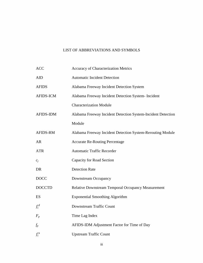
LIST OF ABBREVIATIONS AND SYMBOLS

ACC Accuracy of Characterization Metrics

AID Automatic Incident Detection

AFIDS Alabama Freeway Incident Detection System

AFIDS-ICM Alabama Freeway Incident Detection System- Incident

Characterization Module

AFIDS-IDM Alabama Freeway Incident Detection System-Incident Detection

Module

AFIDS-RM Alabama Freeway Incident Detection System-Rerouting Module

AR Accurate Re-Routing Percentage

ATR Automatic Traffic Recorder

cj Capacity for Road Section

DR Detection Rate

DOCC Downstream Occupancy

DOCCTD Relative Downstream Temporal Occupancy Measurement

ES Exponential Smoothing Algorithm

𝑓𝑓𝑖𝑖𝑑𝑑 Downstream Traffic Count

Fp Time Lag Index

fp AFIDS-IDM Adjustment Factor for Time of Day

𝑓𝑓𝑖𝑖𝑢𝑢 Upstream Traffic Count

iv

FAR False Alarm Rate

FCR False Characterization Rate

FHWA Federal Highway Administration

I Total Number of Adjacent Lanes

IVHS Intelligent Vehicle Highway Systems Program

ISTEA Intermodal Surface Transportation Efficiency Act of 1991

ωm AFIDS-IDM Fuzzy Set Membership Value

GLR Dynamic Model Algorithm

HCP Highway Capacity Manual

ID Road Identification Number

ITS Intelligent Transport Systems Journal

JTR Journal of Transportation Research

(λ) AFIDS-IDM Comparison Value Lambda

LOC Level of Congestion

LOC Index Level of Congestion Index

LOS Level of Service

NCHPP National Cooperative Highway Research Program

𝑜𝑜𝑖𝑖𝑑𝑑 Downstream Occupancy

𝑜𝑜𝑖𝑖𝑢𝑢 Upstream Occupancy

OCC Occupancy at Downstream Detector Station

OCCDF Spatial Occupancy Difference

http://www.trb.org/NCHRP/�

v

OCCRDF Relative Spatial Occupancy Difference

µ𝑆𝑆𝑆𝑆 Degree of Belongingness of the sth Object to the rth Cluster

RGY Red-Green-Yellow Color Scheme

SAFETEA-LU Safe, Accountable, Flexible, and Efficient Transportation Equity

Act: A Legacy for Users

SCDOT South Carolina Department of Transportation

SF Service Flow Rate for AFIDS-IDM LOC

Tn Predetermined Threshold Value

T Time Lag between Upstream and Downstream Sensors

TCRP Transit Cooperative Research Program

TEA-21 Transportation Equity Act for the 21st Century

TMC Traffic Management Center

TRB Transportation Research Board

TTCC Time to Characterize a Cleared Incident

TTCO Time to Characterize an Incident Occurrence

TTD Time to Detect an Incident Occurrence

vs AFIDS-IDM Decision Variable

http://en.wikipedia.org/wiki/Transportation_Equity_Act_for_the_21st_Century�

vi

ACKNOWLEDGMENTS

This research and dissertation effort was completed with the combined efforts and support

of many individuals. First, I would like to thank my dissertation committee chairperson, Dr.

Margaret Rice. Her friendship, guidance, and understanding have been instrumental in the

completion of this work. Over the years, she has been instrumental in the development of my

research skills and interests, for this I owe an enormous debt of gratitude.

I would also like to express my gratitude to Dr. Daniel Fonseca, Dr. Chris Green, Dr. Gary

Moynihan, Dr. Richard Rice, and Dr. Randall Schumacker. Their technical assistance was

invaluable in developing and polishing this research. Without their assistance, this dissertation

could have never been completed.

Special acknowledgement must be extended to The University of Alabama College of

Engineering and The Aging Infrastructure Systems Center of Excellence for the financial support

for this research. Without their support, the cost of this research would have been prohibitive.

On a personal note, I would like to express my gratitude to my family for their unwavering

support over the years that have lead to this effort. Especially, I would like to acknowledge the

support of both my father and sister Donna, whose kind souls and gentle hearts saw the inception

of this program but not its completion.

vii

TABLE OF CONTENTS

CHAPTER PAGE

ABSTRACT ................................................................................................................................ ii

LIST OF ABBREVIATIONS AND SYMBOLS ..................................................................... iii

ACKNOWLEDGMENTS ........................................................................................................ vi

LIST OF TABLES ...................................................................................................................... x

LIST OF FIGURES .................................................................................................................. xii

INTRODUCTION TO THE DISSERTATION .......................................................................... 1

ARTICLE ONE

1.1. Introduction .......................................................................................................................... 9

1.2. Background Studies ........................................................................................................... 11

1.3. Research Objectives and Scope ......................................................................................... 14

1.3.1. Detection Process .................................................................................................... 15

1.3.1.1. Data Set ..................................................................................................... 15

1.3.1.2. Determination of Level of Congestion Index ............................................ 19

1.3.1.3. Determination of Level of Congestion ...................................................... 20

1.3.1.4. Determination of Decision Variable vs ...................................................... 20

1.3.1.5. Determination of Comparison Variable Lambda ...................................... 21

1.3.1.6. Determining Fuzzy Set Membership ........................................................ 22

1.3.1.7. Recognition of Lane Blocking Incident .................................................... 23

1.4. Numerical Tests and Results .............................................................................................. 23

viii

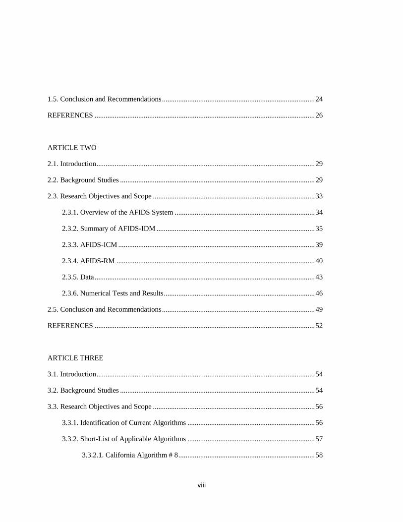
1.5. Conclusion and Recommendations .................................................................................... 24

REFERENCES ......................................................................................................................... 26

ARTICLE TWO

2.1. Introduction ........................................................................................................................ 29



2.3.1. Overview of the AFIDS System ............................................................................. 34

2.3.2. Summary of AFIDS-IDM ....................................................................................... 35

2.3.3. AFIDS-ICM ............................................................................................................ 39

2.3.4. AFIDS-RM ............................................................................................................. 40

2.3.5. Data ......................................................................................................................... 43

2.3.6. Numerical Tests and Results ................................................................................... 46


REFERENCES ......................................................................................................................... 52

ARTICLE THREE

3.1. Introduction ........................................................................................................................ 54



3.3.1. Identification of Current Algorithms ...................................................................... 56

3.3.2. Short-List of Applicable Algorithms ...................................................................... 57

3.3.2.1. California Algorithm # 8 ........................................................................... 58

ix

3.3.2.2. Exponential Smoothing Algorithm ........................................................... 59

3.3.2.3. McMaster Incident Detection Algorithm .................................................. 63

3.3.2.4. Shue Fuzzy Logic Algorithm .................................................................... 65

3.3.2.5. Alabama Freeway Incident Detection System Algorithm ......................... 69

3.3.3. Comparison of Short-Listed Algorithms ................................................................. 73

3.3.3.1. Data ........................................................................................................... 73

3.3.3.2. Comparative Evaluation ............................................................................ 74


REFERENCES ......................................................................................................................... 79

CONCLUSIONS AND RECOMMENDATIONS

Introduction ............................................................................................................................... 82

The Three Articles .................................................................................................................... 82

Further Development ................................................................................................................ 84

Potential Use in Education ........................................................................................................ 85

References for Introduction and Conclusion ............................................................................ 86

APPENDIX A: CODE FOR CALIFORNIA ALGORITHM #8 ..................................... 87

APPENDIX B: CODE FOR EXPONENTIAL SMOOTHING ALGORITHM .......... 115

APPENDIX C: CODE FOR MCMASTER ALGORITHM ........................................... 132

APPENDIX D: CODE FOR SHUE ALGORITHM ....................................................... 151

APPENDIX E: CODE FOR AFIDS-IDM ALGORITHM ............................................. 155

x

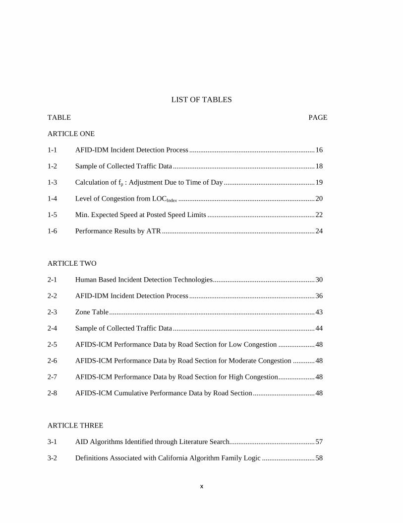
LIST OF TABLES

TABLE PAGE

ARTICLE ONE

1-1 AFID-IDM Incident Detection Process ..................................................................... 16

1-2 Sample of Collected Traffic Data .............................................................................. 18

1-3 Calculation of fp : Adjustment Due to Time of Day .................................................. 19

1-4 Level of Congestion from LOCIndex ........................................................................... 20

1-5 Min. Expected Speed at Posted Speed Limits ........................................................... 22

1-6 Performance Results by ATR .................................................................................... 24

ARTICLE TWO

2-1 Human Based Incident Detection Technologies ........................................................ 30

2-2 AFID-IDM Incident Detection Process ..................................................................... 36

2-3 Zone Table ................................................................................................................. 43


2-5 AFIDS-ICM Performance Data by Road Section for Low Congestion .................... 48

2-6 AFIDS-ICM Performance Data by Road Section for Moderate Congestion ............ 48

2-7 AFIDS-ICM Performance Data by Road Section for High Congestion .................... 48

2-8 AFIDS-ICM Cumulative Performance Data by Road Section .................................. 48

ARTICLE THREE

3-1 AID Algorithms Identified through Literature Search............................................... 57

3-2 Definitions Associated with California Algorithm Family Logic ............................. 58

xi

3-3 Exponential Smoothing Basic Traffic Variables ....................................................... 63

3-4 AFIDS-IDM Incident Detection Process ................................................................... 70


3-6 Road Sections by ATR’s ........................................................................................... 76

3-7 Performance Results for California #8 Algorithm ..................................................... 76

3-8 Performance Results for Exponential Smoothing Algorithm .................................... 76

3-9 Performance Results for McMasters Algorithm ........................................................ 76

3-10 Performance Results for Shue Algorithm .................................................................. 77

3-11 Performance Results for AFIDS-IDM ....................................................................... 77

xii

LIST OF FIGURES

FIGURE PAGE

ARTICLE ONE

1-1 System Flowchart ...................................................................................................... 17

1-2 Road Sections Considered ......................................................................................... 18

ARTICLE TWO

2-1 AFIDS System Flowchart .......................................................................................... 35

2-2 AFIDS-ICM Flowchart .............................................................................................. 41

2-3 AFIDS-ICM Output File............................................................................................ 42

2-4 Detailed AFIDS-ICM Traffic Zone Congestion Status Screen ................................. 42


ARTICLE THREE

3-1 Decision Tree for General Logic of California Algorithm Family ............................ 60

3-2 California #8 Decision Tree Logic ............................................................................ 61

3-3 McMaster Catastrophe Theory Template .................................................................. 64

3-4 Templates Intended for Normal and Recurrent Congestion ...................................... 66


1

INTRODUCTION TO THE DISSERTATION

Problem Statement

In the U.S., evacuations of hundreds of subjects take place every two to three weeks from

disasters such as chemical spills, inclement weather, and terrorist attacks. Major threats from

hurricanes and other natural disasters happen every one to three years, requiring the evacuation

of millions of subjects over short periods of time (TRB No. 29, 2008). Under ideal conditions,

these evacuations are carried out in an orderly manner across pre-planned and well maintained

evacuation routes. However, increased congestion from normal freeway usage has created an

environment where the major thoroughfares normally set aside for evacuation purposes become

stressed as evacuation traffic levels approach near design capacities (Nowakowski, et al., 1999).

These result in traffic patterns overwhelmed by the magnitude of vehicles leaving the affected

area, having detrimental effects on the safety and mobility of vehicles de-departing the

evacuation area.

Hindering the evacuation process, even more, is the potential for non-recurring traffic

incidents. Non-recurring traffic incidents are defined as any incident causing a reduction of

roadway capacity or an abnormal increase in demand, and require first responders to be

dispatched (Coifman, 2007). These incidents further congest the traffic stream by both causing

delays in clean-up efforts by first-responders and increasing the

2

time frame necessary to evacuate subjects from the affected area. Further, they lead to potential

secondary incidents, which result in higher fatality rates.

The combinations of stressed traffic streams and non-recurring and secondary traffic

incidents create delays and backups that result in:

• Increased response time by first responders

• Lost time resulting in a wider evacuation window

• Increased fuel consumption

• Reduced air quality and other adverse environmental conditions

• Increased potential for more serious secondary incidents resulting from rear end

collisions, traffic exiting the route, or exiting to the shoulder of the road

• Increased potential for struck by incidents involving personal responding to

traffic incidents

• Negative public image of first responders involved in incident management

activities

Proposed Solution

This study proposes the Alabama Freeway Incident Detection System (AFIDS) as an

automated decision support system for the recognition and characterization with re-routing

support of non-recurring incidents in evacuation scenarios. The system offers near immediate

incident recognition while providing traffic monitors with a characterization, or priority, scheme

coupled with a re-routing module.

3

AFIDS was developed as an alternative to existing systems after an exhaustive search of

current research related to incident detection and characterization was performed. The proposed

system was deemed necessary due to the need for automatic incident detection that could both

operate with a minimum amount of historical data and be put in place quickly with a minimum

expenditure of time and hardware.

The literature review indicated a trend in the escalating usage of freeway systems resulting

in many freeways operating at near capacity during peak periods (Nowakowski, Green, and

Kojima, 1999). The ensuing traffic patterns associated with these levels of congestion result in

recurrent compression waves that form and break apart over varying periods of time, making the

identification of naturally forming congestion categories somewhat fuzzy. For this reason, fuzzy

set theory, which identifies set membership through degrees of belongingness and allowing

belongingness to multiple sets simultaneously, was determined to be the most appropriate

methodology for real-time incident detection using real data.

AFIDS differs from other automated incident detection systems in that it combines actual

field research reported in the Highway Capacity Manual (HCP) (TRB, 2008) with concepts of

fuzzy cluster analysis. The HCP is a regularly updated composite of multiple years of research

performed by the National Cooperative Highway Research Program (NCHPP), Federal

Highway Administration (FHWA), Transit Cooperative Research Program (TCRP), and

Transportation Research Board (TRB). HCP contains concepts, guidelines, and computational

procedures for computing the capacity and quality of service of various highway facilities.

Fuzzy cluster analysis has been used effectively in data categorization and can be viewed

as an improved clustering methodology (Bezdek, 1973; Hall et. al., 1992; Sugeno and Yasukawa,

1993). This approach to clustering differs from classical clustering techniques in that a given

http://www.trb.org/NCHRP/�

4

data point can be included in multiple groups with the degree of belongingness between 0 and 1.

Classical clustering is defined as the partitioning of a set of S objects into R mutually exclusive

clusters, and can be expressed through an S × R matrix U = [µSR], where µSR = 1 if object s

belongs to the cluster r else µSR = 0.

The discontinuity of clusters, as well as the assurance that clusters are not empty, is

insured in classical clustering techniques through the satisfaction of two conditions:

∑ µ𝑠𝑠𝑠𝑠𝑅𝑅𝑠𝑠=1 = 1, 𝑠𝑠 = 1, … . . , 𝑆𝑆, (1)

µ𝑆𝑆𝑅𝑅 ∊ {0, 1}, 𝑠𝑠 = 1, … . . , 𝑆𝑆; 𝑠𝑠 = 1, … . .𝑅𝑅. (2)

Fuzzy clustering recognizes that exclusive clusters are not necessarily appropriate for

naturally occurring subgroups. In these cases Equation 2 is replaced with

Equation 3:

µ𝑆𝑆𝑅𝑅 ∊ [0, 1], 𝑠𝑠 = 1, … . . , 𝑆𝑆; 𝑠𝑠 = 1, … . .𝑅𝑅. (3)

Where:

the natural subgroup is considered a fuzzy subset of a set of objects

µ𝑆𝑆𝑅𝑅 = the degree of belongingness of the sth object to the rth cluster

When applied to freeway incident detection, fuzzy clustering offers the flexibility to

explain the compression waves or irregular changes in patterns of data attributes that take place

across multiple time frames. This allows the grouping of patterns of lane traffic variables into

5

comparatively like patterns in response to non-recurrent incident effects on real-time freeway

traffic patterns.

Fundamental to fuzzy cluster analysis is the concept of natural subgroups. When the

spatial and temporal relationships of natural subgroups are examined, both the value of fuzzy

cluster analysis and the need for inapproachable spatial and temporal traffic patterns becomes

clear. In this study, this is accomplished by combining fuzzy cluster analysis techniques with the

spatial and temporal traffic patterns and relationships defined in the Highway Capacity Manual

(TRB, 2008).

Current Studies

As part of The University of Alabama College of Engineering, The Aging Infrastructure

Systems Center of Excellence funded the development of the Alabama Freeway Incident

Detection System (AFIDS). AFIDS is a decision support system supporting non-recurrent

incident detection, characterization, and re-routing efforts in Traffic Management Centers

(TMCs).

The three articles in this dissertation define different aspects of the research and evaluation

of the AFIDS project. At the time of this dissertation, a prototype of the system using a modified

version of the incident detection logic has been developed by the Intergraph Corporation.

However, the system has not been implemented in any actual or real setting.

This dissertation is a collection of three articles with introduction and conclusion sections

that summarize the research. Each article is a standalone effort supported with its own literature

review, methodology, and discussion sections. While there is s well defined partition separating

the three works, each article is related to the others through their association with AFIDS.

6

Article One- Traffic Incident Detection Algorithm for Emergency Evacuation Using Real

Data

This article introduces the Alabama Freeway Incident Detection System-Incident

Detection Module (AFIDS-IDM) as a methodology for the detection of freeway incidents.

AFIDS-IDM invokes fuzzy cluster analysis in the identification of lane blocking incidents from

comparisons of time varying patterns of incident induced and incident free traffic states. Lane

traffic counts and density, collected at successive traffic sensors, are the two primary types of

input data. State variables are defined from the spatial and temporal relationships of the raw data,

and then evaluated quantitatively and qualitatively to determine the decision variables necessary

for the determination of lane blocking incidents. The specified decision variable is then

compared to a fuzzy cluster analysis algorithm to determine the existence of a lane blocking

incident.

Article Two- Incident Characterization and Re-routing After Automatic Incident Detection

Article Two defines the Alabama Freeway Incident Detection System- Incident

Characterization Module (AFIDS-ICM) as a methodology for the characterization of previously

identified freeway incidents. The method characterizes incidents through the firing of a series of

fuzzy based rules to determine both partial and full blockage of highway freeways. Freeway

incidents are characterized as “green”, “yellow”, or “red” to indicate severity of traffic

conditions, with red conditions consider the highest priority. When incidents are characterized as

a red condition AFIDS-ICM initiates a computerized rerouting module, the Alabama Freeway

Incident Detection System-Rerouting Module (AFIDS-RM), for the selection of alternate routes

7

using Geo-Media and Geo-Media Web Map. AFIDS-ICM continues to evaluate yellow and red

traffic conditions until a “green” condition exists.

Article Three- Comparison of Five Algorithms for Automatic Freeway Incident Detection

It is the purpose of Article Three to survey current literature related to Automatic Incident

Detection (AID) and to list present methods in this field of study. Further, this article evaluates

each method against a set of criteria to short-list algorithms that are applicable to field practice.

The latter are then implemented using real data collected by the South Carolina Department of

Transportation (SCDOT) to determine the number and location of traffic incidents identified by

each algorithm. The five algorithms selected for comparison are the California Algorithm #8, the

Exponential Smoothing Algorithm, the McMaster Incident Detection Algorithm, the Shue

Algorithm, and the Alabama Freeway Incident Detection System- Incident Detection Module

Algorithm.

Significance and Limitations of the Studies

This initiative will provide traffic officials with relevant insights and expertise to detect

and characterize situations that may drastically impair appropriate responses during a potential

eventuality such as a chemical spill, a terrorist attack, or a natural disaster. The study is limited to

data collected and supplied by the South Carolina Department of Transportation (SCDOT). As

such, only bulk data collected in hourly increments were used. While this impacts the immediacy

of the results, it does not diminish the value of the tool, which applies equally with data collected

at lesser time intervals. The insights of this study are critical to homeland security and

8

emergency management personal who are charged with insuring the safety and security of

numerous individuals through preparedness planning and evacuation.

9

ARTICLE ONE

Traffic Incident Detection Algorithm for Emergency Evacuation Using Real Data

1.1. Introduction

The response to a potential disaster can require the evacuation of personnel from a

specified area. Generally, such efforts are restricted to the orderly mass departure of individuals

across preplanned and well maintained transportation routes. In the U.S., evacuations of up to

1,000 subjects take place every two to three weeks, with more extreme evacuations involving

two million or more every one to three years (TRB, 2008).

While evacuation routes are designed to accommodate normal traffic movements,

congestion and gridlock can occur as the design capacity of the road system is overwhelmed by

the magnitude of vehicles leaving the affected area. The resulting traffic patterns affect the safety

and mobility of subjects moving to more secure areas. Adding to this disarray, potential non-

recurring incidents congest traffic patterns even more. Estimates indicate that between fifty and

sixty-five percent of traffic congestion is caused by non-recurring traffic incidents with an

additional ten percent related to construction and weather (Coifman, 2007). A non-recurring

traffic incident is any event that both causes a reduction of roadway capacity or an abnormal

increase in demand, and requires

10

first responders to be dispatched. Stalled vehicles, roadway debris, spilled loads, and crashes fall

into this category of incidents.

Non-recurring traffic incidents can cause secondary traffic incidents. These incidents

further congest the traffic stream and cause delays in clean-up efforts by first-responders. Studies

indicate that twenty percent of traffic incidents are secondary incidents, with one out of five

resulting in a fatality. In addition to crashes, secondary incidents can include overheated vehicles,

out of fuel conditions, and engine stalls.

The delay and traffic gridlock associated with traffic incidents is compounded during the

evacuation process due to the large numbers of subjects leaving the affected area. These delays

and backups result in:

• Increased response time by first responders

• Lost time resulting in a wider evacuation window

• Increased fuel consumption

• Reduced air quality and other adverse environmental conditions

• Increased potential for more serious secondary incidents resulting from rear end

collisions, traffic exiting the route, or exiting to the shoulder of the road

• Increased potential for struck by incidents involving personal responding to

traffic incidents

• Negative public image of first responders involved in incident management

activities.

11

1.2. Background Studies

Early detection of traffic incidents can both reduce the time to return traffic to normal rates of

flow and reduce the potential for secondary incidents (Busch, 1987), thus increasing the number

of vehicles leaving the affected area. It would be expected, therefore, that the real-time reporting

of traffic data would have dramatic effects on the reduction of the impact of traffic incidents in

emergency evacuations.

A number of methods, both human-based and automated, have been proposed to manage

and regulate traffic movement along freeways (Williams and Guin, 2007). Human-based

methods rely on technologies such as cell phones, call boxes, passing motorists, and first

responder patrols (Monahan, 2007). While these methods are reliable, they are accompanied by a

triggering delay which increases the response time of emergency personnel, further inhibiting

efforts to restore normal traffic movement (Singliar and Hauskrecht, 2006).

Automatic incident detection (AID) is generally founded on a series of algorithms intended

for the detection of freeway incidents. Studies indicate that the effectiveness of AID is, at best,

poor (Parkany and Xie, 2002). The lack of AID operational effectiveness is primarily related to

unacceptably high false alarm rates and complex calibration procedures.

For a period of time, the poor performance of AID was of no consequence, since traffic

management centers (TMCs) were able to provide marginal detection capability through human-

based systems (Sobhi and Kelly, 1999). However, with an estimated 17% of freeways often

experiencing congestion levels at or above capacity, the increasing size and range of freeway

transportation networks are growing at rates faster than human-based resources are capable of

monitoring, bringing a new focus to AID (Nowakowski et al., 1999). It would be expected that

freeway congestion during evacuation would be at or near design capacity, rendering human-

http://findarticles.com/p/search?tb=art&qa=Nazemeh+Sobhi�

http://findarticles.com/p/search?tb=art&qa=Michael+Kelly�

12

based methods incapable of delivering the response time necessary for the significant reduction

of traffic slowdowns related to secondary incidents.

Since the 1960’s, AID has seen a number of advancements. However, inputs have

remained fairly consistent with remotely sensed traffic data as the primary source of

input. Data are zone specific, collected at upstream and downstream sensors for each zone. The

primary metric for most AID algorithms is lane occupancy with others using speed and vehicle

count (Williams and Guin, 2007).

Early efforts in AID were statistical and pattern-based algorithms. These efforts can be

summarized in four categories: comparative algorithms, statistical algorithms, time-series and

filtering based algorithms, and traffic theory based algorithms (Dudek et al., 1974).

Comparative algorithms are characterized by their reliance on pattern recognition for the

identification of patterns of behavior of specific variables known to be associated with incident

conditions. The California algorithm family is an example of this category of algorithms

(Courage and Levin, 1968; Payne and Tignor, 1978). The California family consists of 10

algorithms developed using real traffic data from the Los Angeles freeway system. The

California #8 is one of the more popular algorithms from this group. The algorithm uses decision

tree logic to identify traffic incidents. California algorithms are often used as benchmarks to

evaluate other algorithms.

Statistical algorithms use standard statistical techniques to identify sudden changes in

behavior in variables such as lane occupancy and rate of speed, known to indicate the existence

of an incident (Payne and Tignor, 1978). The Standard Normal Deviate (SND) and Bayesian

Algorithm are examples of these algorithms (Dudek et al., 1974, Courage and Levin, 1968,

Levin and Krause, 1978).

13

Time series and filtering algorithms rely on concepts of time-series to track decision

variables. Incidents are recognized when a decision variable deviates from the modeled time-

series behavior. The Auto-Regressive Integrated Moving Average (ARIMA) based algorithm,

the Exponential Smoothing Algorithm (Cook and Cleveland, 1974), and the Kalman Filtering

based Algorithm are included in this category of algorithms (Chow et al.,1977; Cook and

Cleavland, 1974).

The Exponential Smoothing algorithm was developed for use from data collected from

the John C. Lodge Freeway in Detroit. This method uses double exponential smoothing to

generate a tracking variable that is further processed to recognize a traffic blocking incident.

Traffic theory based algorithms recognize the relationship between the traffic variables as

a means of analysis. The McMaster Algorithm (Persaud et al., 1990; Hall et al., 1993) based on

catastrophe theory, falls in this category. The GLR, a dynamic model algorithm, also falls in this

category. This algorithm is designed to make full use of all information about the dynamic and

stochastic evolution of traffic variables in time and space (Chow et al.1977, Gall and Hall, 1989;

Greene et al., 1977; Kurkijian et al., 1977).

The McMaster Algorithm was developed using data from Queen Elizabeth Way,

Mississauga, Ontario. The basic McMaster Algorithm is a congestion detection algorithm. It uses

a catastrophe theory model for description of the flow-occupancy-

speed relationship. Incidents are detected based on positioning on a flow-density chart.

More recently, AID research and development have moved in the direction of artificial

intelligence and soft computing techniques, ushering in a fifth category of incident algorithms.

Among these are fuzzy logic/fuzzy set theory (Hsiao, Lin, and Cassidy, 1994; Chang and Wang,

1994; Lin and Chang, 1998; Shue, 2002), artificial neural networks (Dia and Rose, 1997), fuzzy

14

logic in conjunction with neural networks (Ishak and AlDeek, 1998a, Ishak and Al-Deek, 1998b,

Srinivasan et al, 2001), fuzzy expert systems (Lin and Chang (1998), wavelet transformations

(Samant and Adeli, 2000), and genetic algorithm over neural networks (Roy and Abdulhai, 2003).

This group of algorithms is referred to as advanced incident detection algorithms.

The development of fuzzy logic/fuzzy set theory algorithms is most promising in that they

do not necessarily rely on complex calibration procedures, but rather on the appraisal of existing

traffic conditions. Additionally, they are principally prepared to deal with the fuzziness of the

complex temporal relationships of ever changing traffic patterns. While advances in this area of

study have been made by Shue (2002), the current state of fuzzy logic/fuzzy set algorithms have

only been tested in simulation and have not been modified to fit real time traffic data.

The large number of approaches to AID indicates an inability of Traffic Management

Center’s (TMC) to settle on one single approach to traffic management. In many cases, the

calibration procedures of more modern algorithms demand technology not available to their

intended users. While issues related to the effectiveness of AID have been addressed in

algorithms developed since the 1990’s, current collection methods employed make these

methodologies difficult to implement.

1.3. Research Objectives and Scope

This paper proposes the Alabama Freeways Incident Detection System- Incident Detection

Module (AFIDS-IDM), an automated method for freeway incident detection, as a necessary tool

for real time incident detection during evacuation processes. AFIDS-IDM is the incident

detection module of the Alabama Incident Detection System (AFIDS). AFIDS is a three module

system consisting of incident detection, incident characterization, and traffic re-routing modules.

15

The proposed system is based on fuzzy set theory. This tool is different from similar tools

on the market in that it is intended for use exclusively in an evacuation process. This increases

the value of the tool by decreasing the complexity of necessary calculations, eliminating the need

for elaborate calibration, and reducing the number of false alarms associated with other

automatic methods. Since the tool is automated, it is expected to reduce the trigger time

associated with the deployment of first responders to traffic incidents. The tool is designed for

use with available TMC technology.

1.3.1 Detection Process

The Alabama Freeway Incident Detection System Incident Detection Module (AFIDS-

IDM) identifies lane blocking incidents from comparisons of time varying patterns of incident

induced and incident free traffic states. Decision variables are defined from the spatial and

temporal relationships of the raw data, and then evaluated quantitatively and qualitatively to

establish inputs for the algorithmic determination of freeway blocking incidents.

The AFID-IDM logic is a continuous loop process carried out in seven steps. These steps

are indicated in Table 1-1. In the event an incident is detected, the system continues to monitor

the location until the incident is cleared up. When no incident is detected, the system continues to

the next time step. This procedure is depicted graphically in

Figure 1-1.

1.3.1.1 Data Set

Data for this study was made available by the South Carolina Department of

Transportation (SCDOT). Vehicle speed and traffic counts from successive upstream and

16

Table 1-1. AFID-IDM Incident Detection Process

Step Description 1 Input data 2 Determination of a Level of Congestion Index (LOC Index) 3 Determination of the Level of Congestion (LOC) from the index 4 Determination of the decision variable vs associated with the specified LOC 5 Determination of the comparison variable lambda (λ) associated with the input data and posted speed limit 6 Determination of the fuzzy set membership, ωm, associated with the specified vs

7 A lane blocking incident exists when ωm > λ.

downstream sensors, or Automatic Traffic Recorders (ATR), collected at hourly intervals were

the primary inputs. Together, the two ATR’s form detection zone. Occupancy values were

calculated mathematically from the data.

The SCDOT data set consisted of data collected over a period of one calendar year from

269 ATR’s across South Carolina. Twelve detection zones, representing continuous sections of

the highway, were selected from this data. Table 1-2 depicts the format in which the collected

data was made available for the study. ID is the road identification number. Hour refers to the

particular hour of the day the data was reported. There are 5 lanes considered for a particular

section of the road. Bin numbers identify the number of vehicles traveling at a given speed. Total

Volume is the summation of the number of vehicles in all the Bins.

Road sections under study, Figure 1-2, were primarily north and south of Greenville along

Interstate Highway 185, north and south of Spartanburg along Interstate Highway 85, and north

and south of Laurens County, along Interstate 385. Data was collected over a period of two and a

half months by SCDOT.

17

ine Decision Variable λ

NO

YES

Figure 1-1. System Flowchart

Start

Input Data

Determine Level of Congestion Index (LOC Index)

Determine Level of Congestion from LOC Index

(Table 3)

Determine Decision

Variable vs

Determine Comparison Variable λ

Determine Fuzzy Set

Membership

ωm(k)

Initiate Characterization Module

ωm(k) > λ

18

Table 1-2. Sample of Collected Traffic Data

ID ATR_ID HOUR LANE Bin_0_5 Bin_11_5 Total Volume ID1 137085 0 1 1 0 0 237 1 137086 0 1 2 0 0 150 2 137087 0 1 3 0 0 31 3 137088 0 1 4 0 0 9 4 137089 0 1 5 0 0 87 5

Figure 1-2. Road Sections Considered

19

1.3.1.2 Determination of Level of Congestion Index

The determination of the Level of Congestion Index (LOC Index), Equation 1-1, is the first

step in the identification of a lane blocking incident. A single algorithm, resulting in a value

between 0 and 1, is necessary to determine the LOC Index

at the upstream and downstream

sensors:

LOC Index ,ijk = ( SFik / cj ) * (1/fp) (1-1)

Where:

LOC Index ,ijk=Level of congestion for i lane of traffic in evacuation route j at time period k

SF = Service flow rate for LOC i under prevailing roadway and traffic conditions for I lanes in

one direction, in vehicles per hour. This value is obtained from the input data, and is the total

number of actual vehicles across all bin numbers for that ATR for that hourly update.

cj = Capacity for the road section under study. This value is obtained from the Capacity field in

the ATR data.

( SFjk / cj ) = Utilization at time factor k.

fp= factor for further adjustments due to time of day (Table 1-3).

Table 1-3. Calculation of fp : Adjustment Due to Time of Day

Traffic Stream Type Factors, fp Weekday or Commuter 1.0 Other 0.75-0.90a

a Engineering judgment and/ local data must be used in selecting the exact value b Reprinted from the Highway Capacity Manual

20

1.3.1.3 Determination of Level of Congestion (LOC)

The LOC Index is applied to Table 1-4 to determine the Level of Congestion (LOC). Posted

speed limit and LOC Index are the two variables in determining the LOC. Congestion categories

are rated as: a) low, b) moderate, c) heavy, and d) over congested.

LOC Categories are derived from Level of Service Categories (LOS) A through F,

described in the Transportation Research Board’s publication Highway Capacity Manual, where:

LOC Category Low = LOS Categories A and B

LOC Category Moderate = LOS Categories C and D

LOC Category High = LOS Category E

LOC Category Over Congestion = LOS Category F.

Table 1-4. Level of Congestion from LOCIndex

50 mph 60 mph 70 mph LOC Category mpvh LOCIndex mpvh LOCIndex mpvh LOCIndex

Low 1,100 0.00-0.54 1,000 0.00-0.69 850 0.00-0.66 Moderate 1,850 0.55-0.93 1,700 0.70-0.84 1,650 0.67-0.83 High 2,000 0.94-1.00 2,000 0.85-1.00 1,900 0.84-1.00 Over Congestion * * * * * * * Highly variable, unstable

1.3.1.4 Determination of Decision variable vs

Decision variable vs is determined through the application algorithms v1, v2, and v3, each

representing the LOC’s low, moderate, and high, respectively.

21

𝑣𝑣𝑖𝑖1(𝑘𝑘) = 𝑜𝑜𝑢𝑢 (𝑘𝑘−𝑛𝑛)− od (𝑘𝑘)𝑜𝑜𝑖𝑖𝑢𝑢 (𝑘𝑘−𝑛𝑛)

(1-2)

𝑣𝑣𝑖𝑖2(𝑘𝑘) = ��𝑓𝑓𝑑𝑑 (𝑘𝑘)𝐽𝐽� − 𝑓𝑓𝑑𝑑(𝑘𝑘)� − {𝑓𝑓𝑑𝑑(𝑘𝑘)/𝐼𝐼} (1-3)

𝑣𝑣𝑖𝑖3(𝑘𝑘) = {𝑓𝑓𝑑𝑑(𝑘𝑘) ∗ 𝑀𝑀𝑖𝑖𝑛𝑛(1.0,𝐹𝐹𝑝𝑝 )} – {𝑓𝑓𝑢𝑢(𝑘𝑘𝑘𝑘−𝑛𝑛) ∗ (𝐶𝐶𝑓𝑓𝑓𝑓 )} – (𝑓𝑓𝑑𝑑 (k))/I (1-4)

Where:

𝑓𝑓𝑖𝑖𝑢𝑢(𝑘𝑘) and 𝑓𝑓𝑖𝑖𝑑𝑑(𝑘𝑘) = the upstream and downstream traffic counts collected at target lane i and

time step k,

𝑜𝑜𝑖𝑖𝑢𝑢(𝑘𝑘) and 𝑜𝑜𝑖𝑖𝑑𝑑(𝑘𝑘) = collected occupancies,

I = total number of adjacent lanes,

T = the maximum time lag predetermined for consideration of the travel time taken from the

upstream detector station to the downstream detector station on the relationship between the

upstream and downstream traffic data,

Fp = time lag index defined as the posted speed limit / distance between 𝑓𝑓𝑖𝑖𝑢𝑢(𝑘𝑘) and

𝑓𝑓𝑖𝑖𝑑𝑑(𝑘𝑘).

1.3.1.5 Determination of Comparison Variable Lambda

Comparison variable λ is determined by offsetting the traffic count at the upstream ATR

by a correction factor adjusting for the minimum speed expected to navigate each detection zone

based on the appropriate LOC. The minimum expected speed values are indicated in Table 1-5.

22

Table 1-5. Min. Expected Speed at Posted Speed Limits at LOC’s High, Moderate, and Low

Posted Speed (mph) 30 35 40 45 50 55 60 65 70 LOC Minimum Expected Speed Low 26 32 38 42 45 48 51 54 57 Moderate 25 32 37 38 40 41 43 44 46 High 23 25 26 27 28 30 30 30 30 Over Congestion * * * * * * * * * * Highly variable, unstable

The comparison value, λ, is arrived through the following equation:

λ = (Upstream traffic count at ATRi) * (Cfs) (1-5)

Where:

Upstream traffic count at ATRi is the vehicle count at time period k determined from the

upstream ATR;

Cfs is a correction factor derived from dividing the minimum expected speed for a detection zone

at a specified LOC by the posted speed for the detection zone.

1.3.1.6 Determining Fuzzy Set Membership

Fuzzy set membership is determined by applying Equation1-6:

ωm (k) = 1 – (vs (k – 𝑓𝑓𝑝𝑝 ) – μm) (1-6)

23

Where:

ωm = Fuzzy set membership value,

μm = pattern of the decision variable pre clustered on the basis of historical traffic data associated

with attribute m, values are as follows:

Low Congestion = 0.75

Moderate congestion = 0.90

Heavy congestion = 1.0

1.3.1.7 Recognition of Lane Blocking Incident

AFIDS-IDM recognizes a lane blocking incident when the following fuzzy rule is fired:

IF 𝜔𝜔𝑚𝑚 (k)>λ THEN a lane blocking incident with attribute m is recognized at time step k ELSE k= k+1 and go back to previous procedure

Where:

m = low, moderate, or high level of congestion category,

k = Specified time frame

1.4. Numerical Tests and Results

Performance tests of the AFIDS-IDM algorithm were conducted with the SCDOT data set.

The results, presented in Table 1-6, indicate that the algorithm successfully identified traffic

incidents in each of the road sections tested.

24

Table 1-6. Performance Results by ATR

Road Section Total Number of Incidents ATR 194-196 5 ATR 196-197 39 ATR 242-243 3 ATR 243-244 2

The total of traffic incidents on road section bounded by ATR’s 196 and 197 were

significantly higher than other road sections. This is attributed to both an overall heavier traffic

count than other road sections and a higher speed limit. The road section bounded by ATR’s 243

and 244 reported the least number of incidents. This section of road was characterized by a much

lower volume of congestion, which explains the lower number of traffic incidents.

1.5. Conclusion and Recommendations

AID research has evolved with the introduction of one technique after another, with no

single methodology assuming a dominate role in incident detection. This is, in some ways,

attributed to the development of many algorithms which take place in simulated environments

where actual traffic conditions were designed to fit the algorithm, giving a greater degree of

control of the experiment than would be found in actual implementation. And where, in other

algorithms, AID methodologies are defined by complex calibrations based on calibration

parameters have to be fine tuned in practice.

This paper introduces the AFIDS-IDM as an alternate methodology for automatic incident

detection based on fuzzy cluster analysis. The algorithm presented was founded in fuzzy

25

clustering and developed around field research defined in the TRB’s Highway Capacity Manual

(2008). The algorithm was tested with real data supplied through the SCDOT. AFIDS-IDM

differs from others in that it is not dependent on the calibration of parameters from historical data.

Performance tests indicate that the algorithm is capable of determining traffic incident

occurrence across a number of different road sections. While the data set provided sufficient

information to allow testing on multiple levels of congestion, it did not provide weather data,

which would have provided greater insight into the performance of the algorithm. This limitation

provides direction for future performance testing for the algorithm.

A limitation of the study was in the data set itself, which was made available in bulk form

at hourly increments. While this is representative of real collection methodologies, this greatly

impaired the evaluation of the algorithm, further providing direction for future research.

26

REFERENCES Busch, F. (Eds). (1987). “Incident Detection”. In M. Papageorgiou (Ed). Concise Encyclopedia of Traffic and Transportation Systems. pp. 219-225. Oxford. Chang, E. C. P. (1994). “Fuzzy Systems Based Automatic Freeway Incident Detection”. IEEE International Conference on Systems, Man, and Cybernetics, San Antonio, Texas, pp. 1727-1733. Chang, E.-P. and Wang, S. H. (1994). "Improved Freeway Incident Detection Using Fuzzy Set Theory". Transportation Research Record, No.1453, pp. 75-82.

Chow, E. Y., Gershwin, S. B., Greene, C. S., Houpt, P. K., Kurkijian, A. and Willsky, A. S. (1977). Dynamic Detection and Identification of Incidents on Freeways Volume I : Summary. ESL-R-764 Electronic Systems Laboratory, Massachusetts Institute of Technology, Cambridge, Massachusetts. Coifman, B.A. (2007). “Distributed Surveillance on Freeways Emphasizing Incident Detection and Verification”. Transportation Research. Part A, Policy and Practice. Volume 41, Issue 8, pp. 750-762. Cook, A. R. and Cleveland, D. E. (1974). "Detection of Freeway Capacity-Reducing Incidents by Traffic-Stream Measurements". Transportation Research Record, No.495, pp. 1-11. Courage, K. G. and Levin, M. (1968). A Freeway Corridor Surveillance, Information and Control System. Research Report 488-8 Texas Transportation Institute, Texas A&M University, College Station. Dia, H. and Rose, G. (1997). “Development and Evaluation of Neural Network Freeway Incident Detection Models Using Field Data”. Transportation Research Part C. Vol.1, No. 3, pp. 203-217. Dudek, C.L., Messer, C.J., Nuckles, N.B. (1974). “Incident Detection on Urban Freeways”. Transportation Research Record 495. TRB, National Research Council, Washington D.C. Dudek , C.L., Weaver , G.D., Ritch, G.P., and Messer, C.J. (1975). “Detecting Freeway Incidents Under Low-Volume Conditions”. Transportation Research Record, No. 533, pp. 34. Gall, A. I. and Hall, F. L. (1989). "Distinguishing Between Incident Congestion and Recurrent Congestion: A Proposed Logic". Transportation Research Record, No.1232, pp. 1-8.

27

Greene, C. S., Houpt, P. K., Willsky, A. S. and Gershwin, S. B. (1977). Dynamic Detection and Identification of Incidents on Freeways Vol. 3 : The Multiple Model Method. ESL-R-766 Electronic Systems Laboratory, Massachusetts Institute of Technology, Cambridge, Massachusetts. Hsiao, C-H., Lin, C-T., and Cassidy, M. (1994). Application of Fuzzy Logic and Neural Networks to Automatically Detect Freeway Traffic Incidents. Journal of Transportation Engineering. Vol. 120, pp. 753-771. Ishak, S. S. and Al-Deek, H. M. (1998a). “Freeway Incident Detection Using Fuzzy Art Adaptive Resonance Theory”. Fifth International Conference on Applications of Advanced Technologies in Transportation Engineering, pp. 59-66.

Ishak, S. S. and Al-Deek, H. M. (1998b). "Fuzzy Art Neural Network Model for Automated Detection of Freeway Incidents". Transportation Research Record, No.1634, pp. 56-63.

Lin, C.-K. and Chang, G.-L. (1998). Development of a Fuzzy-Expert System for Incident Detection and Classification. Mathematical and Computer Modeling. Vol. 27, pp. 9-25. Kurkijian, A., Gershwin, S. B., Houpt, P. K. and Willsky, A. S. (1977). Dynamic Detection and Identification of Incidents on Freeways Volume 2: Approaches to Incident Detection using Presence Detectors. ESL-R-765 Electronic Systems Laboratory, Massachusetts Institute of Technology, Cambridge, Massachusetts. Levin, M. and Krause, G. M. (1978). "Incident Detection: A Bayesian Approach". Transportation Research Record, No.682, pp. 52-58. Lin, W. H. and Daganzo, C. F. (1997). "A Simple Detection Scheme for Delay-Inducing Freeway Incidents". Transportation Research. Part A: Policy and Practice, Vol.31 No.2, pp. 141-155.

Monahan, T. ( 2007). War Rooms of the street: Surveillance practices in transportation control centers. The Communication Review. No. 10, Vol. 4, pp. 367-389. Nowakowski, C., Green, P., Kojima, M. (1999). Human Factors in Traffic Management Centers: A Literature Review. Technical Report UMTRI-99-5, Ann Arbor, MI: The University of Michigan Transportation Research Institute.

Parkany, E. and Xie, C.. (Aug. 2002). “Use of Driver-Based Data for Incident Detection” Seventh International Applications of Advanced Technologies in Transportation Conference, pp. 143-150.

Payne, H. J. and Tignor, S. C. (1978). "Freeway Incident-Detection Algorithms Based on Decision Trees with States". Transportation Research Record, No. 682, pp. 30-37.

28

Roy, P., and Abdulhai, B.(2004). GAID: Genetic Adaptive Incident Detection for Freeways, Journal of the Transportation Research Record, No. 1856, pp 96-106. Samant, A. and Adeli, H. (2001). "Enhancing Neural Network Traffic Incident-Detection Algorithms Using Wavelets". Computer-Aided Civil and Infrastructure Engineering, Vol.16 No.4, pp. 239-245. Shue, J. (2002). A Fuzzy Clustering-Based Approach to Automatic Freeway Incident Detection and Characterization. Fuzzy Sets and Systems. No. 128, pp. 377–388. Singliar, T. and Hauskrecht, M. (2006). “Towards a Learning Traffic Incident Detection System”. ICML Workshop on Machine Learning Algorithms for Surveillance and Event Detection, Pittsburgh. Sobhi, N. and Kelly, M. (1999). Human Factors Recommendations for TMC Design. Public Roads,Vol. 62, No. 6, 36-48. Srinivasan, D., Cheu, R.L., and Poh, Y.P. (2001). “Hybrid Fuzzy Logic-Genetic Algorithm Technique for Automated Detection of Traffic Incidents on Freeways”. 2001 IEEE Intelligent Transportation Systems Conference Proceedings. Oakland (CA). August 25-29. TRB. (2008). The Role of Transit in Emergency Evacuation. Special Report No. 24. Transportation Research Board, Washington, D.C. Williams, B.M. and Guin, A. (June 2007). “Traffic Management Center use of Incident Detection Algorithms: Findings of a Nationwide Survey”. IEEE Transactions on Intelligent Transportation Systems, Vol. 8, No. 2, 351-358.

http://www.cs.pitt.edu/~milos/research/incident-icmlW-2006.pdf�


29

ARTICLE TWO

Incident Characterization and Re-routing After Automatic Incident Detection

2.1. Introduction

Quick and responsive freeway incident detection decreases traffic congestion, fuel

consumption, and environmental pollution. It also reduces the response time of emergency

vehicles, increasing the survival rate of any seriously injured individuals, and minimizes traffic

congestion which can lead to secondary incidents (Lomax et al., 2003). It has, in recent years,

taken on added significance by reducing delays and increasing the number of vehicles evacuated

from hazardous areas. Incident detection in itself, however, is not enough to meet the needs of

stressed highway systems. Characterization and re-routing systems are necessary to organize and

expedite the identification of an existing incident, the determination of its location, and, to

identify alternate routes to alleviate potential traffic buildup (Han and May, 1990).


Incident detection is classified into two categories: human-based and automatic incident

detection (Williams and Guin, 2007). Human-based technologies are primarily dependent on the

reporting of traffic incidents through a number of low tech capabilities such as cell phones and

radios by a number of sources including passing motorists, law enforcement agencies, and

Department of Transportation (DOT) employees (Monahan,

30

2007). These technologies, along with their predominant initiating sources, are outlined in Table

2-1. While considered highly reliable, there is a considerable delay between the occurrence of an

incident and the initiation of a traffic management response where low tech technologies are

engaged (Singliar and Hauskrecht, 2006).

Table 2-1. Human-Based Incident Detection Technologies

Technology Initiating Source Cellular Phone Calls Passing Motorists Freeway Service Patrols Police and Other Official Vehicles Peak Period Patrols Law Enforcement Agencies Fleet Operators DOT Patrol Agents Closed Circuit TV Traffic Center Employees Motorist Call Boxes Passing Motorists Aircraft Patrols Law Enforcement and DOT Fixed Observers Law Enforcement and DOT CB Radio Monitoring Law Enforcement Agencies

Automatic incident detection (AID) is generally founded in a series of algorithms intended

for the recognition of freeway incidents. While this approach has been around since the

beginning of intelligent transportation systems, studies indicate that the effectiveness of AID is,

at best, poor (Parkany and Xie, 2002). The lack of AID operational usefulness is primarily

related to an unacceptably high false alarm rate, resulting in many automatic incident alarms

being either disabled or ignored.

For a period of time, the poor performance of AID was of no consequence, since traffic

management centers (TMCs) were able to provide marginal detection capability through human-

based systems (Sobhi and Kelly, 1999). However, the increasing size and range of freeway

transportation networks under the management of TMCs are growing at rates faster than human-


http://findarticles.com/p/search?tb=art&qa=Michael+Kelly�

31

based resources are capable of monitoring, with an estimated 17% of freeways often

experiencing traffic levels at or above capacity (Nowakowski et al., 1999). This along with the

high cost of building new freeway systems and the passage of bills such as the Safe,

Accountable, Flexible, And Efficient Transportation Equity Act: A Legacy for Users (SAFETEA-

LU) has caused TMCs to face the realization that human-based methods will not meet future

incident detection needs, thereby refocusing attention on AID.

SAFETEA-LU is a bill that governs federal surface road spending (US Government

Printing Office, 2005). In was set in law in August 2005, and will expire in September, 2009. It

is the successor of the Transportation Equity Act for the 21st Century (TEA-21) which followed

the Intermodal Surface Transportation Efficiency Act of 1991 (ISTEA). ISTEA established the

Intelligent Vehicle Highway Systems Program (IVHS). IVHS recognizes the need to link

vehicles and freeways through advanced information systems and the development of Advanced

Traffic Management Systems such as AID (Chen and Galler 1990). This group of bills

recognizes the constraints placed on the further expansion of freeway systems and places a

priority on the maximization of system efficiency and preservation. They also lay out guidelines

for congestion and air quality management.

One of the more progressive aspects of SAFETEA-LU is the recognition of the need for

AID. SAFETEA-LU goes further to recommend that AID be combined with human based

systems. It is expected that this mixture of approaches to incident detection will help overcome

AID shortcomings.

AID is accomplished algorithmically from data collected at sensors strategically located

throughout the control area. The algorithms can be classified through five categories that explain

http://en.wikipedia.org/wiki/Transportation_Equity_Act_for_the_21st_Century�

http://en.wikipedia.org/wiki/TEA-21�

32

the general nature of the algorithm (Dudek and Messer, 1974): a) pattern recognition, b) time

series and filtering, c) statistical, d) traffic theory, and e) advanced algorithms.

Pattern recognition algorithms compare tracking variables against pre-determined

threshold values to identify anomalies. The tracking variable is typically a traffic parameter or a

variable derivative of the traffic parameter (Eisele and Lomax, 2004). Occupancy is the most

common traffic parameter in this class of algorithms. These algorithms are sometimes referred to

as comparative algorithms due to the comparative nature of the variables under consideration.

The California Algorithm family is the most commonly used pattern recognition algorithm

(Courage and Levin, 1968).

In time series and filtering algorithms, the tracking variable is treated as a time-series

variable. In this group of algorithms, an incident is recognized when there is a deviation of the

tracking variable from the modeled time-series behavior. An example of this algorithm is the

exponential smoothing algorithm (Chow et. al., 1977).

Statistical algorithms use typical statistical analysis to identify unexpected changes and

atypical behavior in the tracking variable to identify incidents. Algorithms in this group are

based on the argument that the reverse of a situation is an indication of an incident. Traffic flow,

average speed, and lane occupancy are often used as tracking variables. The Standard Normal

Deviate and the Bayesian define this category of algorithms (Payne and Tignor, 1978).

Traffic theory algorithms rely on relationships between traffic variables for analysis. The

most common of this type of algorithm is the McMaster catastrophe theory algorithm which

determines the state of traffic variables based on its position in a flow-density plot (Chow et al,

1977).

33

Advanced algorithms include a number of algorithms with techniques founded in

advanced mathematical formulae. This category of algorithms integrates inexact reasoning and

uncertainty into the decision logic. Artificial Intelligence methods (AI) are able to recognize

specific patterns and learn from data collected at upstream and downstream sensors, much like

the structure of human thought. AI algorithms are generally founded on either fuzzy logic or

neural networks or combinations of the two (Ishak and Al-Deek, 1998).

The Shue algorithm (Shue, 2002) is a fuzzy clustering based approach to identify lane

blocking incidents from comparisons of time varying patterns of incident induced and incident

free traffic states that was developed in simulation mode. Shue’s approach first recognizes the

existence of a lane blocking incident followed by the characterization of the incident.

The Alabama Freeway Incident Detection System (AFIDS) is an approach to incident

detection similar to the Shue but adapted to the use of real data and specifically designed for use

in evacuation processes. AFIDS consists of three modules: a) incident detection, b) incident

characterization, and b) re-routing. AFIDS is different from other incident detection algorithms

in that it recognizes the slower more congested traffic patterns found in evacuation processes.

And, it was designed around data collection methods in use in Department of Transportation’s

(DOT) around the U.S.

2.3. Research Objective and Scope

It is the purpose of this paper to provide overviews of the AFIDS system and then describe

the AFIDS Incident Characterization (AFIDS-ICM) and re-routing (AFIDS-RM) modules.

AFIDS-ICM and AFIDS-RM are described through the application of real-time data supplied

through the South Carolina Department of Transportation (SCDOT). The AFIDS incident

34

detection module (AFIDS-IDM) is summarized to provide coherency leading to AFIDS-ICM

and AFIDS-RM.

2.3.1 Overview of AFIDS System

The Alabama Freeway Incident Detection System (AFIDS) consists of a three module

automated freeway incident detection, characterization, and re-routing decision support system

employed under emergency evacuation conditions. Alabama Freeway Incident Detection

System-Incident Detection Module (AFIDS-IDM) continuously monitors traffic conditions in

multiple detection zones. Input data, supplied from traffic sensor stations, are processed for the

determination of lane blocking incidents through a fuzzy-clustering algorithm. In the event an

incident is detected, The Alabama Freeway Incident Detection System- Incident Characterization

Module (AFIDS-ICM) is employed. The recognition of an incident causes a change in detection

zone status from normal traffic conditions to a low incident priority. Incidents that persist for

more than one time period are assigned a high priority status; otherwise they are recognized as

cleared and re-assigned a normal condition. When incidents are assigned a high priority status,

GeoMedia Web Map is evoked through the Alabama Freeway Incident Detection System-Re-

routing Module (AFIDS-RM). The module allows Traffic Management Center (TMC) monitors

access to graphical representations of pre-determined routings. These routings represent alternate

routes to alleviate potential traffic congestion caused by the recognized incident. The decision to

re-route traffic along identified routings is at the discretion of TMC monitors. Access to routings

is manually available through lower priority conditions at the discretion on traffic Managers. An

overview of the AFIDS system is depicted graphically in Figure 2-1.

35

No

Yes

No

Yes

Figure 2-1. AFIDS System Flowchart

2.3.2 Summary of AFIDS-IDM

AFIDS-IDM incorporates a fuzzy cluster approach to incident detection with research

findings indentified and reported through the Highway Capacity Manual (TRB, 2008). AFIDS-

IDM follows a seven step approach to incident detection defined in

Table 2-2.

AFIDS Incident Detection Module

(AFIDS-ID)

AFIDS Characterization Module

(AFIDS-IC)

AFIDS Re-Routing Module

(AFIDS-R)

Incident Detected

Re-Route Traffic

36


Step Description 1 Input data 2 The determination of a Level of Congestion Index (LOC Index) 3 The determination of the Level of Congestion (LOC) from the index 4 The determination of the decision variable vs associated with the specified LOC 5 The determination of the comparison variable lambda (λ) associated with the input data and posted speed limit 6 The determination of the fuzzy set membership, ωm, associated with the specified vs


Step 1 is data input. From the data, the LOC Index

2-1.

is determined in Step 2, from Equation

LOCijk = ( SFik / cj ) * (1/fp) (2-1)

Where:

LOCijk = Level of congestion for i lane of traffic in evacuation route j at time period k,

SF = Service flow rate for LOC i under prevailing roadway and traffic conditions for I, lanes in

one direction, in vehicles per hour. This value is obtained from the input data, and is the total

number of actual vehicles across all bin numbers for that ATR for that hourly update,


the ATR data,

( SFjk / cj ) = Utilization at time factor k,

fp= factor for further adjustments due to time of day determined from a look-up table.

37

The LOC Index is applied to a look-up table to determine the Level of Congestion (LOC).

Posted speed limit and LOC Index are the two variables in determining the LOC. Congestion

categories are rated as: a) low, b) moderate, c) heavy, and d) over congested.







A decision variable (vs) and comparison variable (λ) are then defined. Decision variable vs

is determined through the application algorithms v1, v2, and v3, each representing the LOC’s low,

moderate, and high, respectively.

𝑣𝑣𝑖𝑖1(𝑘𝑘) = 𝑜𝑜𝑢𝑢 (𝑘𝑘−𝑛𝑛)− od (𝑘𝑘)

𝑜𝑜𝑖𝑖𝑢𝑢 (𝑘𝑘−𝑛𝑛) (2-2)


𝑣𝑣𝑖𝑖3(𝑘𝑘) = {𝑓𝑓𝑑𝑑(𝑘𝑘) ∗ 𝑀𝑀𝑖𝑖𝑛𝑛(1.0,𝐹𝐹𝑝𝑝 )} – {𝑓𝑓𝑢𝑢(𝑘𝑘𝑘𝑘−𝑛𝑛) ∗ (𝐶𝐶𝑓𝑓𝑓𝑓 )} – (𝑓𝑓𝑑𝑑 (k))/I (2-4)

Where:


time step k,



38




Fp = time lag index defined as the posted speed limit / distance between 𝑓𝑓𝑖𝑖𝑢𝑢(𝑘𝑘) and 𝑓𝑓𝑖𝑖𝑑𝑑(𝑘𝑘).



based on the appropriate LOC.

The comparison value, λ, is arrived through the following equation: λ = (Upstream traffic count at ATRi) * (Cfs) (2-5)

Where:


upstream ATR;



Fuzzy set membership is then determined by applying Equation 2-6:

ωm (k) = 1 – (vs (k – 𝑓𝑓𝑝𝑝 ) – μm) (2-6)

39

Where:


μm pattern of the decision variable pre clustered on the basis of historical traffic data associated

with attribute m.


IF 𝜔𝜔𝑚𝑚 (k)> λ THEN a lane blocking incident with attribute m is recognized at time step k ELSE k= k+1 and go back to previous procedure

2.3.3 AFIDS-ICM

AFIDS-ICM is an automated decision support system designed to provide support to

TMC monitors through a visual display of traffic condition characterizations for traffic

management, or detection, zones monitored by the TMC. Traffic conditions are characterized by

a red-green-yellow (RGY) color scheme where “green” indicates a normal traffic condition,

“yellow” indicates a low priority incident, and “red” indicates a high priority incident. Initial

characterization is a “green” or normal traffic condition. Preliminary detection of freeway

incidents changes the characterization to “yellow” at time step k. Incidents not cleared by k+1 are

re-characterized as “red”. An either, “yellow” or “red” characterization is returned to “green” if

incidents are cleared before the next successive time step. Incident characterization is

incorporated into AFIDS-IDMs IF-THEN-ELSE incident detection logic:

40

CHARACTERIZATION= Green IF 𝜔𝜔𝑚𝑚 (k)> λ at time step k THEN a lane blocking incident with attribute m is recognized at time step k ELSE k= k+1 and go back to previous procedure CHARACTERIZATION= Yellow IF 𝜔𝜔𝑚𝑚 (k)> λ at time step k+1 THEN a lane blocking incident with attribute m is recognized at time step k+1 ELSE k+1= k+2 and go back to previous procedure CHARACTERIZATION= Red

AFIDS-ICM logic is depicted graphically in Figure 2-2.

Traffic characterizations are conveyed to TMC monitors in the form of a visual output file

relying on RGY color schemes. The outputs file (Figure 2-3) is a continuous display monitoring

multiple detection zones with user interface. Clicking on individual RGY color status fields

brings up detailed information associated with the corresponding ATR such as ATR names and

locations (obtained from the revised ATR table) report date, hour (from the ATR data table) and

the traffic congestion status (Figure 2-4). “Red”, or high priority, color fields display a proposed

alternate route, from GeoMedia Web Map.

2.3.4 AFIDS-RM

When incidents are assigned a “Red”, or high priority, traffic congestion status, GeoMedia

Web Map is evoked through the Alabama Freeway Incident Detection System-Re-routing

Module (AFIDS-RM). The module works in conjunction with the AFIDS-ICM Traffic Zone

Congestion Status Screen (Figure 2-4) to allow Traffic Management Center (TMC) monitors

access to graphical representations of pre-determined alternate routings. AFIDS-RM is designed

to support TMC monitors by providing alternate routes to alleviate potential traffic congestion

41

No

Yes

Yes

Yes No No

No Yes No

Figure 2-2. AFIDS-ICM Flowchart

Initial Characterization =

Green (Normal Traffic Conditions)

Incident at Time Step k?

Incident Cleared at

Time Step k+1

Characterization = Yellow

(Preliminary Recognition of Incident)

Characterization = Red

(Incident Continues- Considered High Priority)

Incident Cleared at

Time Step k+2

42

Figure 2-3. AFIDS-ICM Output File

Figure 2-4. Detailed AFIDS-ICM Traffic Zone Congestion Status Screen

43

caused by the recognized incident. Access to routings is manually available through lower

priority conditions at the discretion on traffic Managers.

AFIDS-RM is based of the concept of traffic management, or detection, zones. Automatic

Traffic Recorders (ATR) collect data from upstream and downstream ATR’s to form a single

zone. The data collection network is expanded by adding successive ATR’s where the

downstream ATR for a detection zone becomes the upstream ATR for the next detection zone in

succession. AFIDS-RM establishes the identification and location of ATR’s and their respective

boundaries through a zone layout table

(Table 2-3).

The zone table catalogs GIS reference fields (e.g. Fnode, Tnode, and EdgeID) for use as

GIS references for GeoMedia Web Map. And, to support the color-coding of roadway segments

based on their traffic congestion levels (Figure 2-3 and 2-4).

Table 2-3. Zone Table

Zone # Fnode Tnode FromATRID ToATRID EdgeID Direction 1 2 1 194 196 1 South 2 1 2 197 195 1 North 3 1 5 196 441 7 South 4 5 1 440 197 7 North 5 7 6 345 256 5 East 6 8 7 257 346 5 West

2.3.5 Data

Data input to AFIDS-ICM was supplied by the South Carolina Department of

Transportation. Vehicle speed and traffic counts from successive upstream and downstream

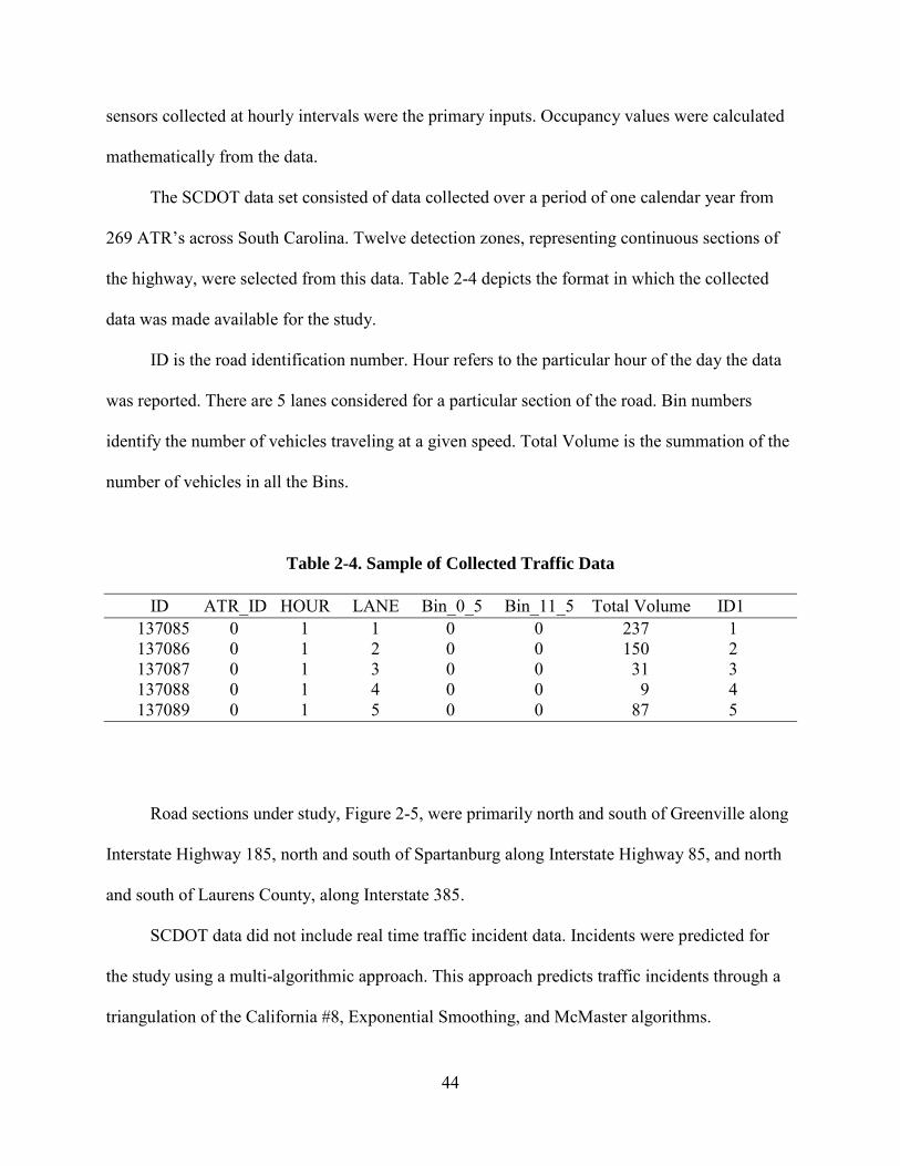
44

sensors collected at hourly intervals were the primary inputs. Occupancy values were calculated

mathematically from the data.

The SCDOT data set consisted of data collected over a period of one calendar year from

269 ATR’s across South Carolina. Twelve detection zones, representing continuous sections of

the highway, were selected from this data. Table 2-4 depicts the format in which the collected

data was made available for the study.

ID is the road identification number. Hour refers to the particular hour of the day the data

was reported. There are 5 lanes considered for a particular section of the road. Bin numbers

identify the number of vehicles traveling at a given speed. Total Volume is the summation of the

number of vehicles in all the Bins.



Road sections under study, Figure 2-5, were primarily north and south of Greenville along

Interstate Highway 185, north and south of Spartanburg along Interstate Highway 85, and north

and south of Laurens County, along Interstate 385.

SCDOT data did not include real time traffic incident data. Incidents were predicted for

the study using a multi-algorithmic approach. This approach predicts traffic incidents through a

triangulation of the California #8, Exponential Smoothing, and McMaster algorithms.

45

For this study, two data sets were formed to predict traffic incident data. Each data set

represented data collected in successive 39 day periods of time. Results of the


California Algorithm was used with the first data set to determine a quadratic equation necessary

to perform the McMaster algorithm. The quadratic equation was then used with the second data

set to predict incidents. The quadratic equation was then determined through the Exponential

46

Smoothing Algorithm using the second data set. The resulting quadratic equation was used to

predict incidents in the first data set. This approach was followed to train the McMaster Incident

Detection Algorithm with the first data set, and use the McMaster Algorithm to detect incidents

with the second data set.

2.3.6. Numerical Tests, and Results

Results of characterization and re-routing algorithms fit eight categories:

1. Correct recognition and assignment of “green” traffic congestion conditions.

2. Incorrect recognition and assignment of “green” traffic congestion conditions.

3. Correct recognition and assignment of “yellow” traffic congestion conditions.

4. Incorrect recognition and assignment of “yellow” traffic congestion conditions.

5. Correct recognition and assignment of “red” traffic congestion conditions.

6. Incorrect recognition and assignment of “red” traffic congestion conditions.

7. Correct identification of alternate traffic routes.

8. Incorrect identification of alternate traffic routes.

AFIDS-ICM and AFIDS-RM results are defined through three objectives:

1. Maximize the correct characterization of real-time incidents

2. Minimize the number of false characterizations

3. Maximize the correct number of alternate routes reported

47

Objectives are evaluated through three metrics: FCR, DR, and AR. The FCR is the false

characterization rate, which reports the percentage of incorrect characterizations as a percentage

of total characterizations. The DR is the detection rate. Reported as a percentage, the DR is an

indicator of the number of characterizations that remain undetected. The AR is the correct

number of re-routings reported by AFIDS-RM. The AR is expressed as a percentage.

The accuracy of FCR, DR, and AR are indicated by the ACC. The ACC (Equation 2-7) is

expressed as a percentage of correct assignments and places the FCR, DR, and AR on a common

scale.

ACCn = 𝑁𝑁𝑢𝑢𝑚𝑚𝑁𝑁𝑁𝑁𝑁𝑁 𝑜𝑜𝑓𝑓 𝐶𝐶𝑜𝑜𝑁𝑁𝑁𝑁𝑁𝑁𝐶𝐶𝐶𝐶 𝐴𝐴𝑓𝑓𝑓𝑓𝑖𝑖𝐴𝐴𝑛𝑛𝑚𝑚𝑁𝑁𝑛𝑛𝐶𝐶𝑓𝑓𝑇𝑇𝑜𝑜𝐶𝐶𝑇𝑇𝑇𝑇 𝑁𝑁𝑢𝑢𝑚𝑚𝑁𝑁𝑁𝑁𝑁𝑁 𝑜𝑜𝑓𝑓 𝐴𝐴𝑓𝑓𝑓𝑓𝑖𝑖𝐴𝐴𝑛𝑛𝑚𝑚𝑁𝑁𝑛𝑛𝐶𝐶𝑓𝑓

𝑋𝑋 100 (2-7)

A fourth metric, the time to characterize (TTCn) is introduced as a means to distinguish the

time to characterize occurring incident across levels of congestion from the time to characterize

an incident that has cleared. The time to characterize an incident that has occurred (TTCO) is the

time to detect and characterize an incident from the time the incident occurs until it is detected

and characterized. The time to characterize a cleared incident (TTCC) is the time to recognize the

characterization of a cleared incident from the time it is cleared until it is no longer recognized as

an incident.

Tables 2-5 through 2-7 summarize AFIDS-ICM performance data for road sections I-185,

I-385, and I-85; described in Section 2.5 and indicated in Figure 2-5. The performance data is

grouped by the LOC’s low, moderate, and high; representing the various levels of congestion

acknowledged by the study. Table 2-8 represents the average performance data for all levels of

congestion by road section.

48

Table 2-5 AFIDS-ICM Performance Data by Road Section for Low Congestion

LOC Low TTCO TTCC DR FCR AR ACC Rd. Sec. (m) (m) (%) (%) (%) (%) I-85 12.8 32.2 100 0 100 100 I-185 13.8 31.2 100 0 100 100 I-385 13.8 31.2 100 0 100 100

Table 2-6 AFIDS-ICM Performance Data by Road Section

for Moderate Congestion

LOC M oderate TTCO TTCC DR FCR AR ACC Rd. Sec. (m) (m) (%) (%) (%) (%) I-85 12.9 31.1 100 0 100 100 I-185 13.8 31.2 100 0 100 100 I-385 13.8 31.2 100 0 100 100

Table 2-7 AFIDS-ICM Performance Data by Road Section for High Congestion

LOC High TTCO TTCC DR FCR AR ACC Rd. Sec. (m) (m) (%) (%) (%) (%) I-85 24.4 20.6 100 0 100 100 I-185 24.9 20.1 100 0 100 100 I-385 24.9 20.1 100 0 100 100

Table 2-8 AFIDS-ICM Cumulative Performance Data by Road Section

LOC All LOC’s TTCO TTCC DR FCR AR ACC Rd. Sec. (s) (s) (%) (%) (%) (%) All Rd. Sec. 17.2 27.65 100 0 100 100

49

Results indicated in Tables 2-5 through 2-7, and summarized in 2-8, support the use of

AFIDS-ICM and AFIDS-RM as a means of characterization of traffic incidents and the

identification of alternate routes as an integral part of traffic related decision support. Using a

computer based platform, the methodologies described result in characterization and re-routing

within 24.4 minutes for low and high priority incidents. And, 32.2 minutes for cleared incidents.

ACC results support that all three objectives of the study were obtained and that the two

modules operate at maximum efficiency. This is somewhat expected due to the incorporation of

computer logic into the process that all but eliminates the possibility for error.

The TTCn is relatively high compared to other approaches. However, this relates to the

efficiency of the AFIDS-IDM, which is tuned for maximum identification of incidents with

limited tolerance for false alarms. Such tuning is achieved through a calculation process that

waits longer to make a decision, but is less prone to error.

There is a noticeable difference between the times to characterize a cleared incident

(TTCC) and the time to characterize an incident that has occurred (TTCO). This is explained on

the basis of fuzzy clustering theory where an incident can only be declared “cleared” when the

decision variable reaches an incident free state. That is the degree of belongingness associated

with the incident-free membership is greater than the degree of belongingness associated with

the incident membership. This, greater than relationship, can only be obtained at the expense of

increased time.

2.5. Conclusion and Recommendations

Advances in AID have lead to a number of approaches to automatic incident detection.

These approaches were generally restricted to incident detection and stopped short of incident

50

characterization and re-routing options. This has created a void in traffic control and

management efforts, leading to increased legislation directed toward the creation of advanced

information systems linked to freeways and vehicles.

This paper introduces AFIDS-ICM as the incident characterization module of the AFIDS

decision support system. The system is augmented with a re-routing module, AFIDS-RM,

employed when high priority incidents are recognized. The modules presented engage traffic

management personnel through a series of user friendly computer screens that are color coded to

simplify the recognition and characterization of traffic incidents.

Performance tests of the two modules indicate that the modules meet their intended

objectives through the:

1. Maximization of the real time characterization of traffic incidents

2. Minimization of the number of false characterizations

3. Maximization of the correct number of correct alternate routes reported

In comparison to alternative approaches to incident characterization and re-routing, the

two modules described offer two relative advantages:

1. The two modules presented are accompanied with an incident detection capability.

Working in unison, the three modules form a complete decision support system directed

toward the identification and characterization of traffic incidents, supported with re-

routing capability.

51

2. The two modules are supported with color coded computer graphic output for incident

detection and graphical mapping for re-routing.

Current efforts are underway to enhance the computer graphic capability of the two

modules. Through these efforts, traffic managers will be able to access additional screens

detailing historical data, weather conditions, traffic flows is areas surrounding the incident, and

weather conditions surrounding the incident. This is expected to increase the value of the tool by

providing additional decision support data.

52

REFERENCES

Busch, F. (Eds). (1987). “Incident Detection”. In M. Papageorgiou (Ed). Concise Encyclopedia of Traffic and Transportation Systems, pp. 219-225. Oxford. Chen, K. & Galler, B. (1990). “An Overview of Intelligent Vehicle-Highway Systems (IVHS) Activities in North America”. Proceedings of the Fifth Jerusalem Conference on Information technology. Jerusalem, Israel. Pp. 694 – 701. Chow, E. Y., Gershwin, S. B., Greene, C. S., Houpt, P. K., Kurkijian, A. and Willsky, A. S. (1977). Dynamic Detection and Identification of Incidents on Freeways Volume I : Summary. ESL-R-764 Electronic Systems Laboratory, Massachusetts Institute of Technology, Cambridge, Massachusetts. Courage, K. G. and Levin, M. (1968). A Freeway Corridor Surveillance, Information and Control System. Research Report 488-8 Texas Transportation Institute, Texas A&M University, College Station. Dudek, C.L. and Messer, C.J. (1974). “Incident Detection on Urban Freeways”. Transportation Research Record, No. 495, pp. 12–24. Eisele, W.L., and Lomax, T.J. (2004). ODOT Operations Performance Measures: Final Report. Sponsored by the Oregon Department of Transportation, June 2004. Available at: http://mobility.tamu.edu/resources. Ishak, S. S. and Al-Deek, H. M. (1998). “Freeway Incident Detection Using Fuzzy Art Adaptive Resonance Theory”. Proc. Fifth International Conference on Applications of Advanced Technologies in Transportation Engineering, pp. 59-66. Lomax, T.J., Turner, S.M., and Margiotta, R. (2003). Monitoring Urban Roadways in 2001: Examining Reliability and Mobility with Archived Data. Report FHWA-OP-03-041. Pp. 64. Monahan, T. ( 2007). War Rooms of the street: Surveillance practices in transportation control centers. The Communication Review Iss. 10, No. 4, pp. 367-389. Nowakowski, C., Green, P., Kojima, M. (1999). Human Factors in Traffic Management Centers: A LiteratureRreview. (Technical Report UMTRI-99-5), Ann Arbor, MI: The University of Michigan Transportation Research Institute. Parkany, E. and Xie, C.. (Aug. 2002). “Use of Driver-Based Data for Incident Detection”. Proceedings of the 7th International Applications of Advanced Technologies in Transportation Conference, pp. 143-150.

53

Payne, H. J. and Tignor, S. C. (1978). "Freeway Incident-Detection Algorithms Based on Decision Trees with States". Transportation Research Record, No.682, pp. 30-37. Roy, P., and Abdulhai, B.(2004). “GAID: Genetic Adaptive Incident Detection for Freeways”. Transportation Research Record, No. 1856, pp 96-106. U.S, Government Printing Office. (2005). Safe, Accountable, Flexible, Efficient Transportation Equity Act: A Legacy for Users (SAFETEA-LU), Title V, Subtitle C, Sec. 5301-5310. Washington, DC: U.S. Government Printing Office. Shue, J. (2002). A Fuzzy Clustering-Based Approach to Automatic Freeway Incident Detection and Characterization. Fuzzy Sets and Systems, Iss. 128, pp. 377–388. Singliar, T. and Hauskrecht, M. (2006). “Towards a Learning Traffic Incident Detection System”. ICML 2006 Workshop on Machine Learning Algorithms for Surveillance and Event Detection, Pittsburgh. Sobhi, N. and Kelly, M. (1999). Human Factors Recommendations for TMC Design. Public Roads, Vol. 62, No.6, pp. 36-48. Transportation Research Board. (2008). Highway Capacity Manual (3rd ed.), Washington, DC: National Academy of Sciences. Williams, B.M. and Guin, A. (June 2007). “Traffic Management Center use of Incident Detection Algorithms: Findings of a Nationwide Survey”. IEEE Transactions on Intelligent Transportation Systems, Vol. 8, no. 2, pp. 351-358.




54

ARTICLE THREE

Comparison of Five Algorithms for Automatic Freeway Incident Detection

3.1. Introduction

Non-recurring traffic incidents can be costly, resulting in increased traffic congestion, fuel

consumption, and environmental pollution. Some estimates place these costs in excess of $35

billion per year (Lindley, 1996). Early recognition can help control the escalation of costs by

both reducing the time frame to clear an incident and reducing the potential for secondary

incidents (Busch, 1987). It is not unexpected that a considerable body of research has evolved on

quick detection methodologies centered on automatic incident detection (Williams and Guin,

2007).


The beginnings of Automatic Incident Detection (AID) can be traced back to the 1960’s

with early approaches restricted to the development of statistical and pattern-based algorithms

(Dudek and Messer, 1974; Courage and Levin, 1968; Levin and Krause, 1978). Since that time,

other efforts, based on numerous approaches, have evolved. These include comparative

algorithms (Payne and Tignor, 1978), time series and filtering algorithms (Chow et al.1977;

Cook and Cleveland, 1974), and traffic theory based algorithms (Chow et al.1977; Gall and Hall,

1989; Greene et al., 1977; Kurkijian et al., 1977).

55

More recently, AID research has centered on artificial intelligence and soft computing

techniques producing a number of methodologies including fuzzy logic/fuzzy set theory (Hsiao

et al., 1994; Chang and Wang, 1994; Lin and Chang, 1998; Shue, 2002), artificial neural

networks (Dia and Rose, 1997), fuzzy logic in conjunction with neural networks (Ishak and Al-

Deek, 1998; Srinivasan et al, 2001), fuzzy expert systems (Lin and Chang, 1998), wavelet

transformations (Samant and Adeli, 2000), and generic algorithms over neural networks (Roy

and Abdulhai, 2003).

AID research has evolved with the introduction of one technique after another, with no

single methodology assuming a dominate role in incident detection. This can be somewhat

perplexing for traffic management practitioners who must distinguish the applicability of one

approach over another in actual field applications. Compounding the issue further is that many

methods were developed in simulated environments where actual traffic conditions were

designed to fit the algorithm, giving a greater degree of control of the experiment than would be

found in actual implementation. Further, AID methodologies are generally presented as

standalone approaches rather than as comparisons against baseline values.

One barrier to comparison by field practitioners is the complex calibrations that many AID

are based on. The calibration parameters have to be fine-tuned in practice. Failure to do so

properly can result in poor performance and abnormally high false alarm rates (Balke, 1993).

Data collection appears to be the single commonality to AID. Lane traffic counts and

density, collected at successive traffic sensors, are the two primary types of input data. Capacity

is then calculated mathematically from inputs.

The evaluation of incident detection algorithms is a somewhat time consuming process,

due to the need to calculate threshold values for each methodology. However, since incident

56

detection algorithms seldom perform at the levels they were developed under (Abdulhai and

Ritchie, 1999), it is a necessary undertaking. The standard approach that has evolved to meet this

need produces three metrics (Dia et al., 996): a) detection rate (DR), false alarm rate (FAR), and

time to detect (TTD). The Comparison of AID’s between detection zones is through a

methodology assigning weighted priorities to each of the three metrics.

3.3. Research Objectives and Scope

It is the purpose of this paper to survey current literature related to AID and to list present

methods in this field of study. Further, this paper evaluates each method against a set of criteria

to short-list algorithms that are applicable to field practice. The latter are then implemented using

real data collected by the South Carolina Department of Transportation (SCDOT) to determine

the FAR, DR, and TTD.

3.3.1 Identification of Current Algorithms

The literature search included a wide variety of electronic and print resources to identify

algorithms for inclusion in this study, including the Transportation Research Board (TRB), the

Journal of Transportation Research (JTR), and the Intelligent Transport Systems Journal (ITS).

Additionally, holdings from seven university libraries and Dissertation Abstracts International

were searched along with reference sections of the innumerable studies that were collected were

reviewed to identify other potential pertinent research. Finally, several researchers and

practitioners, currently working in the field, were contacted and asked to provide pertinent

research or to identify sources of studies.

A total of twenty-two algorithms, indicated in Table 3-1, were identified from the

57

Table 3-1. AID Algorithms Identified Through Literature Search

________________________________________________________________________ Standard Normal Deviate Algorithm Exponential Smoothing Algorithm Low Volume Algorithm Dynamic Model (MM and GLR) The California Algorithms Bayesian Decision Logic Units-based Algorithm HIOCC and PATREG ARIMA Multi-Layer Feed-Forward DELOS Image Processing Fuzzy Logic Principal Component Analysis Cumulative Sum of Occupancy Probabilistic Neural Network Algorithm

Fuzzy Radial Neural Network Algorithm Adaptive ANN-Wavelet Algorithm Wavelet Energy-Radial Basis Algorithm Discrete Wavelet Transform Algorithm CUSUM based Algorithm Support Vector Machine

literature review. Inclusion criteria for the initial list centered on its ability to recognize traffic

incidents and not on its applicability to TMC’s.

3.3.2 Short-List of Applicable Algorithms

The twenty-two algorithms were examined for five unique identifiers to determine if they

met criteria for inclusion in the study. The criteria, listed below, identify those algorithms that

can be implemented with real traffic data:

• Over-saturation is not included as a category of analysis

• The capability to analyze bulk data on an hour-by-hour basis

• Incidents are predicted within a specific zone at a given point in time

• No traffic incident data was available for the fine tuning of the algorithm

• Lane occupancy could be calculated mathematically

58

Five algorithms met the criteria for inclusion:

• California Algorithm #8

• Exponential Smoothing Algorithm

• McMaster Incident Detection Algorithm

• Shue Fuzzy Logic Algorithm

• Alabama Freeway Incident Detection System Algorithm

3.3.2.1 California Algorithm #8

The California Algorithm Family (Payne and Tignor, 1978) is a set of 10 algorithms that

are founded in decision tree analysis. The original algorithm is a straightforward approach

recognizing a potential incident has occurred when three tests on the measured occupancy from

two adjacent stations surpass preset threshold values (Tn) associated with each test. Definitions

associated with the general logic of the California Algorithm Family are presented in Table 3-2

followed by a graphical representation of the logic in decision tree form in Figure 3-1.

Table 3-2. Definitions Associated with California Algorithm Family Logic

Measure Description Definition OCC(i,t) Occupancy at detector station i at time t DOCC(i,t) Downstream occupancy OCC(i+1,t) OCCDF(i,t) Spatial occupancy difference OCC(i,t) - DOCC(i,t) OCCRDF(i,t) Relative spatial occupancy difference OCCDF(i,t) / OCC(i,t) DOCCTD(i,t) Relative temporal downstream (DOCC(i,t-2)-OCC(i,t) occupancy difference /OCC(i,t-2)) Tn Predetermined threshold value

59

An incident state is terminated when threshold value T2 is no longer exceeded. Threshold

values are calibrated from empirical data.

The simplicity of the original algorithm resulted in an unacceptably high false alarm rate.

Subsequent algorithms reduce the false alarm metric but are more complex.

The two that have demonstrated higher performance ratings are the #7 and #8. The

California #7 replaces the use of relative temporal differences in downstream occupancy values

with occupancy measurements (DOCCTD(i,t)). This reduces the false alarm rate through the

recognition of recurring compression waves commonly found in heavy traffic. The #7 recognizes

that simple downstream occupancy data dropping below a certain threshold, usually 20 percent is

more indicative of an incident. This algorithm also incorporates a persistence check that requires

traffic discontinuity persist for a specified period of time before a potential incident is

recognized.

The California #8 is the most complex of the California family and it has been shown to be

the best performer (Cohen and Ketselidou, 1993). The algorithm recognizes nine states and

requires the calibration of five threshold values, two more than previous algorithms. This

algorithm introduces a repetitive test for compression waves and a suppression of alarms related

to these waves for up to five minutes. Through this approach, the #8 is less likely to give a false

alarm in normal traffic congestion. The modified decision logic of the California #8 is presented

in Figure 3-2 as suggested by Payne et al. (1976).

3.3.2.2 Exponential Smoothing Algorithm

The Exponential Smoothing Algorithm was developed by Cook (1974) using data from the

John C. Lodge Freeway in Detroit. The method is an extension of the Standard Normal Deviate

60

Figure 3-1. Decision Tree for General Logic of California Algorithm Family

61

Figure 3-2. California #8 Decision Tree Logic

States: 0- Incident Free Condition 5- Compression wave 5 minutes ago 1- Compression wave this minute 6- Tentative incident 2- Compression wave 2 minutes ago 7- Incident confirmed 3- Compression wave 3 minutes ago 8- Incident continuing 4- Compression wave 4 minutes ago

62

Algorithm (Dubek, and Messer, 1974) but differs in the use of a more sophisticated forecasting

method. The smoothing feature of the algorithm gives a heavier weight to recent traffic data than

past records reducing false alarms related to traffic volumes. The algorithm uses a double

smoothing approach indicated in Equations 3-1 and 3-2.

S1(k) = X(k) + (1- S1(k-1) ( 3-1)

S2(k) = S1(k) + S2 (k-1) (3-2)

Where:

X= A smoothing constant determined from the weight of past data

S1= The first set of smoothed data

S2= The second set of smoothed data

k= Time step

The smoothed data set is then used to generate a tracking signal as the algebraic sum of all

previous estimate errors to the present minute, divided by the current estimate of the standard

deviation. An incident is indicated when the tracking signal deviates from zero beyond a pre-

specified threshold. The threshold can be computed based on either the variability of the data or

likelihood of a false alarm.

Cook used a set of 13 traffic variables resulting from the basic traffic variables of volume,

occupancy, and speed to test the performance of the algorithm (Cook and Cleveland, 1974). The

variables are indicated in Table 3-3.

63

Table 3-3. Exponential Smoothing Basic Traffic Variables

Station volume Subsystem volume Station occupancy Subsystem occupancy Station speed (volume/occupancy) Subsystem speed Station volume-occupancy Subsystem kinetic energy Station speed-occupancy Volume-occupancy discontinuity Station kinetic energy Speed-occupancy discontinuity Station discontinuity

3.3.2.3 McMaster Incident Detection Algorithm

The McMaster Incident Detection Algorithm is a catastrophe theory algorithm developed

using data from Queen Elizabeth Way, Mississauga, Ontario. The algorithm is based on the

belief that flow and occupancy, unlike speed, change smoothly when moving from a congested

to an uncongested state. The algorithm starts by identifying congested states, and then, it

attempts to determine if the congestion is the cause of a traffic incident or a permanent

bottleneck. As suggested by Persaud et al. (1981) a volume-occupancy template (Figure3-3) is

derived from historical flow-occupancy data collected at times of change from congested to

uncongested conditions. Traffic conditions are classified into one of four states, calibrated at

each detector station:

State 1- Uncongested

State 2- Congestion

State 3- Congestion

State 4- Permanent bottleneck congestion

64

State Description: 1- Uncongested 3- Congestion 2- Congestion 4- Permanent bottleneck congestion

Figure 3-3. McMaster Catastrophe Theory Template

Once the volume-occupancy template is determined the following logic is applied:

1. If State 2 or 3 is indicated the algorithm examines the traffic condition at the downstream

station.

2. An alarm is triggered if the downstream station is in State 1 or 2 on the belief that

recurring and incident congestion result in different downstream traffic patterns.

3. If State 3 is detected the algorithm looks at the next downstream detector station using

the same logic.

4. If State 4 is detected at the downstream detector station, the congestion is classified as

recurring.

65

The initial McMaster algorithm was refined to include additional states intended to

decrease the vulnerability of the algorithm to incident related traffic patterns resulting from non-

incident conditions. This modified the original logic to include separate templates to discriminate

between detector stations, depending on their location with respect to recurring bottlenecks. As

suggested by Hall et al. (1993), Figure 3-4 indicates the templates, intended for normal and

recurrent congestion stations.

Calibration of the algorithm involves distinguishing between the congested and un-

congested regions. The minimum non-congested speed is estimated for the station. This is used

to create the boundary between States 1 and 3. A quadratic equation is then estimated to obtain

flow as a function of occupancy at the station, and a constant flow value is estimated, which is to

be subtracted from the function to create the boundary between States 1 and 2.

3.3.2.4 Shue Fuzzy Logic Algorithm

The Shue algorithm (Shue, 2002) is a fuzzy clustering approach to freeway incident

detection and characterization developed under simulation of traffic patterns through CORSIM.

The method identifies lane blocking incidents from comparisons of time varying patterns of

incident induced and incident free traffic states. Lane traffic

counts and density, collected at successive traffic sensors, are the two primary types of input

data.

The Shue algorithm is carried out in four steps:

1. Identification of traffic flow conditions

2. Determination of decision variable

66

Figure 3-4. Templates Intended for Normal and Recurrent Congestion

Template Indicating Typical Parameters for Normal Station

Template Indicating Typical Station Affected by Recurrent Congestion

67

3. Determination of fuzzy set membership

4. Determination of a lane blocking incident

Step one is a pre-classification of traffic flow conditions as low, moderate, heavy, or over

congestion. Each condition is assigned an occupancy based threshold determined through

historical data. At a given time-step, the time varying occupancy based correlation associated

with each type of traffic condition is calculated with lane occupancies collected at the upstream

sensor along with the occupancy-based threshold. Comparisons of the time-varying occupancy

based correlation values indicate the specific type of flow condition in accordance with the

highest correlation value identified by the time varying occupancy values.

Incident occurrence is recognized through the execution of Steps 2 through 4. In Step 2, a

decision variable is determined for the previously identified traffic condition. The decision

variables for low, moderate, and heavy congestion are determined through equations 3-3, 3-4,

and 3-5 respectively. No decision variable is determined for over congestion:

𝑣𝑣𝑖𝑖5 (k) = [𝑜𝑜𝑖𝑖𝑢𝑢 (𝑘𝑘)− 𝑜𝑜𝑖𝑖

𝑑𝑑 (𝑘𝑘)]𝑜𝑜𝑖𝑖𝑢𝑢 (𝑘𝑘)

(3-3)

𝑣𝑣𝑖𝑖 4 (𝑘𝑘) = {[[∑ 𝑓𝑓𝑗𝑗𝑑𝑑𝐽𝐽𝑗𝑗=1 (𝑘𝑘)]/𝐽𝐽] − 𝑓𝑓𝑖𝑖𝑑𝑑(𝑘𝑘)} {[ ∑ 𝑓𝑓𝑗𝑗𝑑𝑑

𝐽𝐽𝑗𝑗=1 (𝑘𝑘)]/𝐽𝐽} (3-4)

𝑣𝑣𝑖𝑖 10(𝑘𝑘) = �∑ 𝑓𝑓𝑖𝑖𝑑𝑑𝑇𝑇𝜏𝜏 (𝑘𝑘 − 𝜏𝜏)� − 𝑓𝑓𝑖𝑖𝑢𝑢(𝑘𝑘 − 𝑇𝑇) −

∑ 𝑓𝑓𝑗𝑗𝑑𝑑 (𝑘𝑘)𝐽𝐽

𝑗𝑗=1

𝐽𝐽 (3-5)

Where:

𝑓𝑓𝑖𝑖𝑢𝑢 (𝑘𝑘)𝑎𝑎𝑎𝑎𝑑𝑑 𝑓𝑓𝑖𝑖𝑑𝑑 (𝑘𝑘)= the upstream and downstream traffic counts collected at target lane i and time step k, 𝑜𝑜𝑖𝑖 𝑢𝑢 𝑎𝑎𝑎𝑎𝑑𝑑 𝑜𝑜𝑖𝑖 𝑑𝑑 = collected occupancies,

68

J = total number of adjacent lanes, T = the maximum time lag predetermined for consideration of the travel time taken from the upstream detector station to the downstream detector station on the relationship between the upstream and downstream traffic data, τ = time lag index. Step 3 computes a time varying decision-variable correlation, Equation 3-6, for upstream,

midstream, and downstream locations on a lane by lane basis. The decision variable measures the

association between decision variables calculated in Step 2 to pattern clusters determined

through historical data.

𝜔𝜔𝑚𝑚 ,𝑎𝑎 𝑝𝑝 .𝑞𝑞 (𝑘𝑘) = 1 − 1

𝛣𝛣�∑ (𝑣𝑣𝑎𝑎𝑠𝑠3

𝜏𝜏=0 (𝑘𝑘 − 𝜏𝜏) − µ𝑚𝑚 ,𝑎𝑎𝑝𝑝 .𝑞𝑞 )2 (3-6)

Where:

β = a pre-determined value set for the boundaries of 𝜔𝜔𝑚𝑚 ,𝑎𝑎 𝑝𝑝 .𝑞𝑞 (𝑘𝑘),

m = level of congestion,

n = lane code,

p = location parameter indicating the location being investigated,

q = a binary digit (q1 = incident occurrence and q0 = no incident),

µ𝑚𝑚 ,𝑎𝑎𝑝𝑝 .𝑞𝑞 = pattern of the decision variable pre clustered on the basis of historical traffic data

associated with attributes p, q, m, and n.

An incident is recognized in Step 4 when the following condition is met:

IF {Max[𝜔𝜔𝑚𝑚 ,𝑎𝑎1,1 (𝑘𝑘),𝜔𝜔𝑚𝑚 ,𝑎𝑎

2,1 (𝑘𝑘),𝜔𝜔𝑚𝑚 ,𝑎𝑎3,1 (𝑘𝑘)]− 𝜔𝜔𝑚𝑚 ,𝑎𝑎

𝑝𝑝 ,0 (𝑘𝑘)} > 𝜆𝜆1 THEN A lane-blocking incident with the attributes m and n is recognized at time step k

69

Where:

m = low, moderate, or high level of congestion category;

n = lane code,

k = Specified time frame.

3.3.2.5 Alabama Freeway Incident Detection System (AFIDS) Algorithm

The Alabama Freeway Incident Detection System (AFIDS) is a three module approach to

incident detection, characterization, and re-routing in emergency evacuation situations. Incident

detection is through a single module, Alabama Freeway Incident Detection System- Incident

Detection Module (AFIDS-IDM). AFIDS-IDM incorporates a fuzzy cluster approach to incident

detection is an extension of the Shue algorithm. The primacy differences between the two

algorithms lies in the environments in which they were developed and the intended application.

The Shue algorithm was developed through a simulated environment using Corridor Simulation

(CORSIM) software for use in normal freeway incident detection. AFIDS, on the other hand,

was developed from freeway data from the South Carolina Department of Transportation

(SCDOT) for use in emergency evacuation situations. This difference is compounded in that

AFIDS centers on real world traffic patterns and states while the Shue was developed on traffic

patterns and states defined through simulation. The patterns and states defining AFIDS are

identified through the Transportation Research Record.

AFIDS-IDM logic, Table 3-4, is carried out in seven steps. Like most fuzzy set algorithms,

AIDS does not give a clear incident or no-incident signal but rather the likelihood that an

incident has occurred. The fuzzy logic incorporated into the algorithm is designed to

approximate human thinking in situations of imperfect knowledge.

70


Step Description 1 Input data 2 The determination of a Level of Congestion Index (LOC Index) 3 The determination of the Level of Congestion (LOC) from the index 4 The determination of the decision variable vs associated with the specified LOC 5 The determination of the comparison variable lambda (λ) associated with the input data and posted speed limit 6 The determination of the fuzzy set membership, ωm, associated with the specified vs


Step 1 is data input. From the data, the LOC Index

3-7.

is determined in Step 2, from Equation

LOCijk = ( SFik / cj ) * (1/fp) (3-7)

Where:

LOCijk = Level of congestion for i lane of traffic in evacuation route j at time period k,

SF = Service flow rate for LOC i under prevailing roadway and traffic conditions for I, lanes in

one direction, in vehicles per hour. This value is obtained from the input data, and it is the total

number of actual vehicles across all bin numbers for that ATR for that hourly update,


the ATR data,

( SFjk / cj ) = Utilization at time factor k,

fp= factor for further adjustments due to time of day determined from a look-up table.

71

The LOC Index is applied to a look-up table to determine the Level of Congestion (LOC).

Posted speed limit and LOC Index are the two variables in determining the LOC. Congestion

categories are rated as: a) low, b) moderate, c) heavy, and d) over congested.







Decision variable vs is determined through the application algorithms v1, v2, and v3, each

representing the LOC’s low, moderate, and high, respectively.

𝑣𝑣𝑖𝑖1(𝑘𝑘) = 𝑜𝑜𝑢𝑢 (𝑘𝑘−𝑎𝑎)− od (𝑘𝑘)

𝑜𝑜𝑖𝑖𝑢𝑢 (𝑘𝑘−𝑎𝑎)

(3-8)


𝑣𝑣𝑖𝑖3(𝑘𝑘) = {𝑓𝑓𝑑𝑑(𝑘𝑘) ∗ 𝑀𝑀𝑖𝑖𝑎𝑎(1.0,𝐹𝐹𝑝𝑝 )} – {𝑓𝑓𝑢𝑢(𝑘𝑘𝑘𝑘−𝑎𝑎) ∗ (𝐶𝐶𝑓𝑓𝑠𝑠 )} – (𝑓𝑓𝑑𝑑 (k))/I (3-10)

Where:


time step k,



72




Fp = time lag index defined as the posted speed limit / distance between 𝑓𝑓𝑖𝑖𝑢𝑢(𝑘𝑘) and 𝑓𝑓𝑖𝑖𝑑𝑑(𝑘𝑘).



based on the appropriate LOC.

The comparison value, λ, is arrived through the following equation: λ = (Upstream traffic count at ATRi) * (Cfs) (3-11)

Where:


upstream ATR;



Fuzzy set membership is determined by applying Equation 3-12:

ωm (k) = 1 – (vs (k – 𝑓𝑓𝑝𝑝 ) – μm) (3-12)

Where:


73

μm = pattern of the decision variable pre clustered on the basis of historical traffic data associated

with attribute m.


IF 𝜔𝜔𝑚𝑚 (k)> λ THEN a lane blocking incident with attribute m is recognized at time step k ELSE k= k+1 and go back to previous procedure

3.3.3. Comparison of Short-Listed Algorithms

Twenty-two incident detection algorithms were identified through an extensive literature

review. The algorithms were evaluated against a set of criteria to determine a short-list of

algorithms applicable to field application. This list included the California Algorithm #8,

Exponential Smoothing Algorithm, McMaster Incident Detection Algorithm, Shue Fuzzy Logic

Algorithm, and Alabama Freeway Incident Detection System Algorithm. The effectiveness of

the five algorithms was compared against a set of metrics accepted in the evaluation of incident

detection algorithms.

3.3.3.1 Data

Data from 269 sensors across South Carolina was made available for the study. Out of

these, 12 detection zones, representing continuous sections of the highway, were selected. Data

were obtained in terms of vehicle speed and traffic counts from upstream and downstream

sensors. Two sensors, or Automatic Traffic Recorders (ATR), in succession define a detection

zone. Occupancy values are mathematically calculated from the data. The format in which the

collected data was made available for the study is presented in Table 3-5.

74

ID is the road identification number. Hour refers to the hour of the day the data was

reported number sequentially. Lanes indicates the specific lane under consideration and the

number lanes in the specific section of road. Bin numbers indicate the number of vehicles

traveling at a given speed. Total Volume is the summation of vehicles across all Bins.

Road sections under study, Figure 3-5, were primarily north and south of Greenville, S.C.,

along Interstate Highway 185, north and south of Spartanburg, S.C., along Interstate Highway

85, and north and south of Laurens County, S.C., along Interstate 385. Data was collected over a

period of two and a half months by SCDOT.



3.3.3.2 Comparative Evaluation

Each of the short-listed algorithms was evaluated to determine the number of incidents

each identified across four road sections taken from the data set. Each road section formed a

detection zone and was bounded by upstream and downstream ATR’s. The road sections and

ATR’s forming the detection zones are presented in Table 3-6. Incident detection results are

presented in Tables 3-7 through 3-11.

75


76

Table 3-6. Road Sections by ATR’s

Road Section # Upstream ATR Downstream ATR 1 194 196 2 196 197 3 242 243 4 243 244

Table 3-7. Performance Results for California #8 Algorithm


Table 3-8. Performance Results for Exponential Smoothing Algorithm


Table 3-9. Performance Results for McMasters Algorithm


77

Table 3-10. Performance Results for Shue Algorithm


Table 3-11. Performance Results for AFIDS-IDM


Performance results indicate that the Exponential Smoothing, Shue, and AFIDS-IDM

algorithms report similar results. This indicates that the sensitivity of the three algorithms is

tuned to pick up similar categories of incidents across a range of severities. The California #8

and McMasters algorithms, on the other hand, indicate that they are tuned to detect only more

severe incidents.

Results indicate that the rankings of incident occurrence for the five algorithms are

identical, with ATR’s 196-197 reporting the most incidents followed by ATR’s 194-196. ATR’s

243-244 reported the least number of incidents in the AFIDS-IDM algorithm, while the

McMasters reported the least number of incidents through ATR’s 242-243. The remaining three

algorithms reported equal incidents from ATR’s 242-243 and ATR’s 243-244.

78

3.4 Conclusion and Recommendations

This research surveyed current literature related to AID, to list present methods in this

field of study. These methodologies were then compared to a set of criteria to determine a short-

list of algorithms relevant to field practice. Each of the five algorithms represented a different

methodology in automatic incident detection. The five algorithms identified were then

implemented with data made available from the South Carolina Department of Transportation

(SCDOT) to determine the number of incidents detected by each algorithm.

Of the short-listed algorithms, the Exponential Smoothing (ES), Shue, and AFIDS-IDM

algorithms performed at similar sensitivities. The California #8 and McMasters algorithms were

noticeably less sensitive than other algorithms.

A limitation of this research lies in its reliance on a single data set. More research is

needed with the short-listed algorithms using more diverse data sets demonstrating more varied

traffic patterns across significantly different weather patterns.

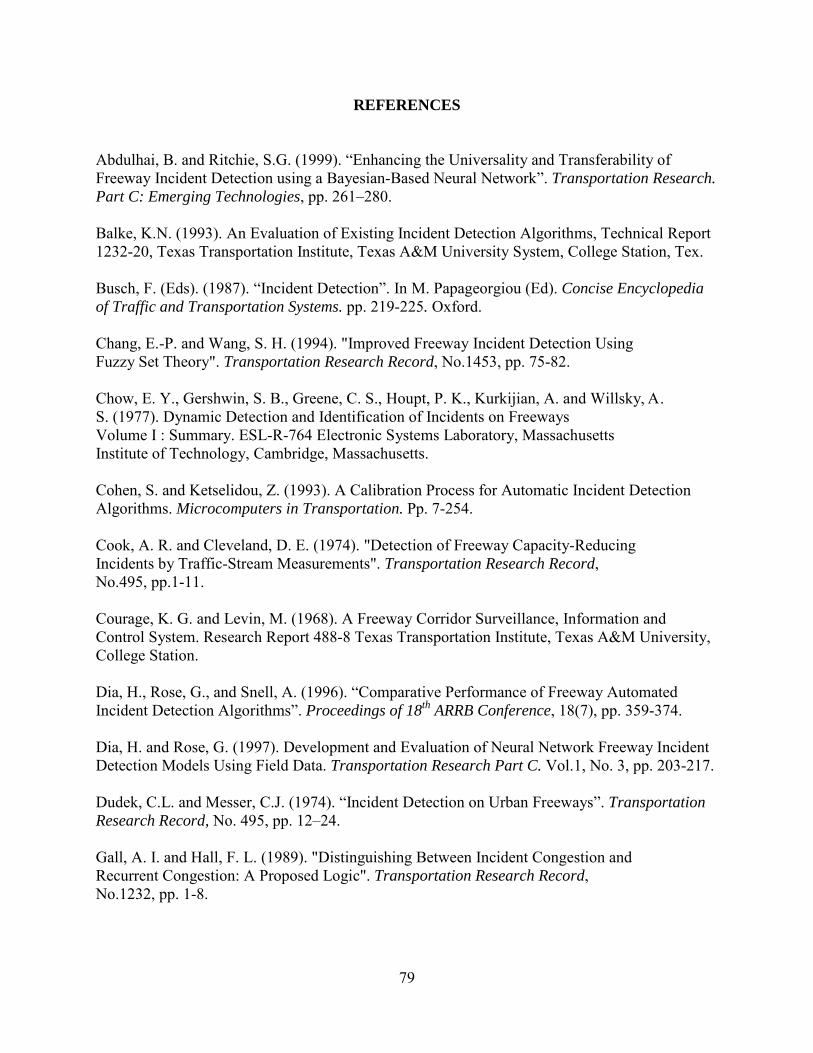
79

REFERENCES

Abdulhai, B. and Ritchie, S.G. (1999). “Enhancing the Universality and Transferability of Freeway Incident Detection using a Bayesian-Based Neural Network”. Transportation Research. Part C: Emerging Technologies, pp. 261–280. Balke, K.N. (1993). An Evaluation of Existing Incident Detection Algorithms, Technical Report 1232-20, Texas Transportation Institute, Texas A&M University System, College Station, Tex. Busch, F. (Eds). (1987). “Incident Detection”. In M. Papageorgiou (Ed). Concise Encyclopedia of Traffic and Transportation Systems. pp. 219-225. Oxford. Chang, E.-P. and Wang, S. H. (1994). "Improved Freeway Incident Detection Using Fuzzy Set Theory". Transportation Research Record, No.1453, pp. 75-82.

Chow, E. Y., Gershwin, S. B., Greene, C. S., Houpt, P. K., Kurkijian, A. and Willsky, A. S. (1977). Dynamic Detection and Identification of Incidents on Freeways Volume I : Summary. ESL-R-764 Electronic Systems Laboratory, Massachusetts Institute of Technology, Cambridge, Massachusetts. Cohen, S. and Ketselidou, Z. (1993). A Calibration Process for Automatic Incident Detection Algorithms. Microcomputers in Transportation. Pp. 7-254.

Cook, A. R. and Cleveland, D. E. (1974). "Detection of Freeway Capacity-Reducing Incidents by Traffic-Stream Measurements". Transportation Research Record, No.495, pp.1-11. Courage, K. G. and Levin, M. (1968). A Freeway Corridor Surveillance, Information and Control System. Research Report 488-8 Texas Transportation Institute, Texas A&M University, College Station. Dia, H., Rose, G., and Snell, A. (1996). “Comparative Performance of Freeway Automated Incident Detection Algorithms”. Proceedings of 18th ARRB Conference, 18(7), pp. 359-374. Dia, H. and Rose, G. (1997). Development and Evaluation of Neural Network Freeway Incident Detection Models Using Field Data. Transportation Research Part C. Vol.1, No. 3, pp. 203-217. Dudek, C.L. and Messer, C.J. (1974). “Incident Detection on Urban Freeways”. Transportation Research Record, No. 495, pp. 12–24. Gall, A. I. and Hall, F. L. (1989). "Distinguishing Between Incident Congestion and Recurrent Congestion: A Proposed Logic". Transportation Research Record, No.1232, pp. 1-8.

80

Greene, C. S., Houpt, P. K., Willsky, A. S. and Gershwin, S. B. (1977). Dynamic Detection and Identification of Incidents on Freeways Volume 3: The Multiple Model Method. ESL-R-766 Electronic Systems Laboratory, Massachusetts Institute of Technology, Cambridge, Massachusetts. Hall, F. L., Shi, Y., and Atala, G. (1993). Off-Line Testing of the McMaster Incident Deteciton Algorithm Under Recurrent Congestion. Transportation Research Record, No. 1394, pp. 1-7, TRB, National Research Council, Washington D.C. Hsiao, C-H., Lin, C-T., and Cassidy, M. (1994). Application of Fuzzy Logic and Neural Networks to Automatically Detect Freeway Traffic Incidents. Journal of Transportation Engineering. Vol. 120, No. 5, pp. 753-771. Ishak, S. S. and Al-Deek, H. M. (1998). "Fuzzy Art Neural Network Model for Automated Detection of Freeway Incidents". Transportation Research Record, No.1634, pp. 56-63. Kurkijian, A., Gershwin, S. B., Houpt, P. K. and Willsky, A. S. (1977). Dynamic Detection and Identification of Incidents on Freeways Volume 2 : Approaches to Incident Detection using Presence Detectors. ESL-R-765 Electronic Systems Laboratory, Massachusetts Institute of Technology, Cambridge, Massachusetts. Lin, C.-K. and Chang, G.-L. (1998). Development of a Fuzzy-Expert System for Incident Detection and Classification. Mathematical and Computer Modeling. Vol. 27, No. 9-11, pp. 9-25. Lindley, J. A. (1996). Qualication of Urban Freeway Congestion and Analysis of Remedial Measures, Technical Report RD/87-052, FHWA, Washington, D.C. Payne, H.J., Helfenbein, E.D., and Knobel, H.C. (1976). Development and Testing of Incident-Detection Algorithms: Vol. 2, Research Methodology and Detailed Results, Technical Report FHWA-RD-76-12, Federal Highway Administration, Washington, DC. Payne, H. J. and Tignor, S. C. (1978). "Freeway Incident-Detection Algorithms Based on Decision Trees with States". Transportation Research Record, No.682, pp. 30-37. Persaud, B.N., Hall, F.L., and Hall, L.M. (1981). Congestion Identification Aspects of the McMaster Incident Detection Algorithm. Transportation Research Record No. 1287. Pp. 167-175. Roy, P., and Abdulhai, B.(2004). “GAID: Genetic Adaptive Incident Detection for Freeways”. Transportation Research Record No. 1856, pp 96-106, Samant, A. and Adeli, H. (2001). "Enhancing Neural Network Traffic Incident-Detection Algorithms Using Wavelets". Computer-Aided Civil and Infrastructure Engineering, Vol.16 No.4, pp. 239-245.

81

Shue, J. (2002). A Fuzzy Clustering-Based Approach to Automatic Freeway Incident Detection and Characterization. Fuzzy Sets and Systems, No. 128, pp. 377–388.

Srinivasan, D., Cheu, R.L., and Poh, Y.P. (2001). “Hybrid Fuzzy Logic-Genetic Algorithm Technique for Automated Detection of Traffic Incidents on Freeways”. 2001 IEEE Intelligent Transportation Systems Conference Proceedings. pp. 25-29. Oakland (CA). Williams, B.M. and Guin, A. (June 2007). “Traffic Management Center use of Incident Detection Algorithms: Findings of a Nationwide Survey”. IEEE Transactions on Intelligent Transportation Systems, No. 8, Vol. 2, pp. 351-358.

82

CONCLUSIONS AND RECOMMENDATIONS

Introduction

This study, written in journal article form, presents three papers centered on automatic

incident detection. Working in building block fashion, each article addresses the subject from a

different perspective. As a whole the three papers form a coherent body of knowledge that

introduce a new methodology, define a method for its implementation, and compare the method

to others in the field.

The Three Journal Articles

Article One- Traffic Incident Detection Algorithm for Emergency Evacuation Using Real

Data

This article introduces the Alabama Freeway Incident Detection System-Incident

Detection Module (AFIDS-IDM) as a methodology for the detection of freeway incidents.

AFIDS-IDM incorporates fuzzy cluster analysis with traffic research reported in the 2008

Highway Capacity Manual in the identification of lane blocking incidents from comparisons of

time varying patterns of incident induced and incident free traffic states. Lane traffic counts and

density, collected at successive traffic sensors, are the two primary types of input data. State

variables are defined from the spatial and temporal relationships of the raw data, and then

evaluated quantitatively and qualitatively to determine the decision variables necessary for the

determination of lane blocking

83

incidents. The specified decision variable is then compared to a fuzzy cluster analysis algorithm

to determine the existence of a lane blocking incident.

AFIDS-IDM was evaluated using data supplied through the South Carolina Department of

Transportation (SCDOT). Performance results indicate that AFIDS-IDM was able to identify

traffic incidents across a range of road sections.

Article Two- Incident Characterization and Re-routing After Automatic Incident Detection

Article Two defines the Alabama Freeway Incident Detection System- Incident

Characterization Module (AFIDS-ICM) as a methodology for the characterization of traffic

incidents identified by the AFIDS-ID. The method characterizes incidents through the firing of a

series of fuzzy based rules that prioritize traffic zones as “green”, “yellow”, or “red” to indicate

severity of traffic conditions, with red conditions consider the highest priority. The Alabama

Freeway Incident Detection System-Rerouting Module (AFIDS-RM) is employed when "red”

incidents are recognized. This module selects alternate routes using Geo-Mapping. Users are

presented with a decision support system with computer based interface as a means of

implementing AFIDS-ICM and AFIDS-RM.

Article Three- Comparison of Five Algorithms for Automatic Freeway Incident Detection

It is the purpose of Article Three to survey current literature related to Automatic Incident

Detection (AID) and to list present methods in this field of study. A short list of algorithms is

determined from a set of criteria designed to identify algorithms capable of implementation to

real-world traffic incident detection. The algorithms are then implemented using real data

collected by the South Carolina Department of Transportation (SCDOT) to determine the

84

number and location of traffic incidents identified by each algorithm. The five algorithms

selected for comparison are the California Algorithm #8, the Exponential Smoothing Algorithm,

the McMaster Incident Detection Algorithm, the Shue Algorithm, and the Alabama Freeway

Incident Detection System- Incident Detection Module Algorithm.

Further Development

Further development of the study presented through this dissertation lies in its boundaries.

As such, a number of limitations become apparent. Chief among these is the use of the single

South Carolina Department of Transportation (SCDOT) data set, and the limited resources made

available to Department of Transportation (DOT) users.

The chief limitation of the study lies in the South Carolina Department of Transportation

(SCDOT) data set, which was somewhat incomplete in that it did not provide the actual traffic

incident data necessary for the determination of real-time false alarm rates (FAR), detection rates

(DR), and mean time to detect incident (MTTD), nor did it provide data in any means other than

at hourly intervals. While this data is seldom maintained by Department of Transportations

(DOTs), simulation offers the prospect of making reasonable determinations from combinations

of computer-generated traffic conditions and actual DOT data sets that allow the determination

of these metrics. It would be expected then, that this work would be extended using this

methodology.

A second limitation of the study lies in the use of a single data set. This restricts the testing

of the proposed methodology by presenting a limited exposure to climatic and seasonal changes

that impact traffic patterns. Additional research is needed in testing the methodology with data

sets that exhibit extreme conditions to test the limits of the methodology.

85

While the methodology presented is in a plain and uncomplicated form, it is the result of

the infant nature of the proposed system. This is obvious from the limited support provided to

end users. Additional development is needed in the identification and incorporation of supporting

information such as weather conditions surrounding occurred incidents, congestion of adjoining

traffic arteries, and location of first responders. This information can be invaluable in the routing

of first responders to incident areas.

Potential Use in Education

The proposed methodology has a number of uses within the educational community. Chief

among these are the disproportional number of evacuations that plague the educational

community and the vulnerability of school age students to real or perceived danger.

Because the majority of school age students are congregated in relatively close spaces

without immediate transportation, issues related to inclement weather and other issues often

necessitate their evacuation to safer locations. This creates a need to insure that any resulting

traffic incidents be recognized as quickly as possible to facilitate their clean up and return of

traffic to normal conditions.

Failure to insure the safe evacuation of school age students can result in an increased

perception of the immediate situation that can grow into hysteria, adding to the value of the

propose system to the school system. The immediate recognition and characterization of

incidents can lead to an increased sense of security for those being evacuated.

86

REFERANCES

Bezdek, J.C. (1973). Fuzzy Mathematics in Pattern Classification. Ph.D. diss., Cornell University. Hall, L.O., Bensaid, A.M. Clarke, L.P., Velthuizen, R.P., Silbiger, M.S., and Bezdek, J.C. (1992). A Comparison of Neural Network and Fuzzy Clustering techniques in Segmenting Magnetic Resonance Images of the Brain. IEEE Trans. Neural Networks, Vol. 3, No. 5, pp. 672–682. Nowakowski, C., Green, P., Kojima, M. (1999). Human Factors in Traffic Management Centers: A Literature Review. (Technical Report UMTRI-99-5), Ann Arbor, MI: The University of Michigan Transportation Research Institute. Sugeno, M. and Yasukawa, T. (1993). A Fuzzy-Logic-Based Approach to Qualitative Modeling, IEEE Trans. Systems Vol.24, No. 6, pp. 1279–1284. Transportation Research Board. (2008). Highway Capacity Manual (3rd ed.), Washington, DC: National Academy of Sciences.

87

APPENDIX A

CODE FOR CALIFORNIA ALGORITHM #8

j=1;

for i=1:3:4103

occa(j)=a(i)/(a(i)+a(i+1)+a(i+2));

occa(j+1)=a(i+1)/(a(i)+a(i+1)+a(i+2));

occa(j+2)=a(i+2)/(a(i)+a(i+1)+a(i+2));

j=j+3;

end

j=1;

for i=1:3:4103

occb(j)=b(i)/(b(i)+b(i+1)+b(i+2));

occb(j+1)=b(i+1)/(b(i)+b(i+1)+b(i+2));

occb(j+2)=b(i+2)/(b(i)+b(i+1)+b(i+2));

j=j+3;

end

88

j=1;

for i=1:3:4103

lanea1(j)=a(i);

lanea2(j)=a(i+1);

lanea3(j)=a(i+2);

j=j+1;

end

j=1;

for i=1:3:4103

laneb1(j)=b(i);

laneb2(j)=b(i+1);

laneb3(j)=b(i+2);

j=j+1;

end

k=1;

j=1;

l=1;

89

for i=1:24:660

for k=1:24

olaneaa1(l,k)=occa(i);



k=k+1;

i=i+1;

end

l=l+1;

end

k=1;

j=1;

l=1;

for i=1:24:660

for k=1:24

olanebb1(l,k)=occb(i);


90


j=j+1;

k=k+1;

i=i+1;

end

l=l+1;

end

k=1;

j=1;

l=1;

for i=1:24:660

for k=1:24

laneaa1(l,k)=lanea1(i);



k=k+1;

i=i+1;

91

end

l=l+1;

end

k=1;

j=1;

l=1;

for i=1:24:660

for k=1:24

lanebb1(l,k)=laneb1(i);



j=j+1;

k=k+1;

i=i+1;

end

l=l+1;

end

92

%

% THRESHOLD VALUES

%

% T1=0;

count=0;

k=1;

l=1;

pt1=0

pt2=0

for i=1:28

for j=3:24

OCCDF(i,j)=lanebb1(i,j)-laneaa1(i,j);

if OCCDF(i,j)>398

OCCRDF(i,j)=OCCDF(i,j)/laneaa1(i,j);

if OCCRDF(i,j)>5

DOCCTD(i,j)=(lanebb1(i,j-2)-lanebb1(i,j))/lanebb1(i,j-2);

if DOCCTD(i,j)>0.1540

93

count=count+1;

i;

j;

pt1(l)=olanebb1(i,j);

pt2(l)=lanebb1(i,j);

l=l+1

% plot(olanebb1(i,j),lanebb1(i,j),'-o')

% hold on

end

end

end

end

end

count

pt1

pt2

% a=[0.4124,0.4097,0.4066]

94

% b=[554,496,456]

% % FOR SECTION OF ROAD FROM ATR_ID_196 TO ID_197 %

%

% j=1;

% for i=1:3:5399

% occa(j)=a(i)/(a(i)+a(i+1)+a(i+2));

% occa(j+1)=a(i+1)/(a(i)+a(i+1)+a(i+2));

% occa(j+2)=a(i+2)/(a(i)+a(i+1)+a(i+2));

% j=j+3;

% end

% j=1;

% for i=1:3:4103

% occb(j)=b(i)/(b(i)+b(i+1)+b(i+2));

% occb(j+1)=b(i+1)/(b(i)+b(i+1)+b(i+2));

% occb(j+2)=b(i+2)/(b(i)+b(i+1)+b(i+2));

% j=j+3;

% end

95

% j=1

% for i=1:3:5399

% lanea1(j)=a(i);

% lanea2(j)=a(i+1);

% lanea3(j)=a(i+2);

% j=j+1;

% end

% j=1;

% for i=1:3:4103

% laneb1(j)=b(i);

% laneb2(j)=b(i+1);

% laneb3(j)=b(i+2);

% j=j+1;

% end

% % j

% k=1;

% j=1;

96

% l=1;

% for i=1:24:1368

% for k=1:24

% olaneaa1(l,k)=occa(i);



% k=k+1;

% i=i+1;

% end

% l=l+1;

% end

% k=1;

% j=1;

% l=1;

% for i=1:24:1368

% for k=1:24

% olanebb1(l,k)=occb(i);

97



% j=j+1;

% k=k+1;

% i=i+1;

% end

% l=l+1;

% end

% k=1;

% j=1;

% l=1;

% for i=1:24:1368

% for k=1:24

% laneaa1(l,k)=lanea1(i);



% k=k+1;

98

% i=i+1;

% end

% l=l+1;

% end

% k=1;

% j=1;

% l=1;

% for i=1:24:1368

% for k=1:24

% lanebb1(l,k)=laneb1(i);



% j=j+1;

% k=k+1;

% i=i+1;

% end

% l=l+1;

99

% end

% % l

% % %

% % %

%

% % T1=0;

% count=0;

% k=1;

% for i=1:57

% for j=3:24

% OCCDF(i,j)=lanebb1(i,j)-laneaa1(i,j);

% if OCCDF(i,j)> 268

% OCCRDF(i,j)=OCCDF(i,j)/laneaa1(i,j);

% if OCCRDF(i,j)>3.92

% DOCCTD(i,j)=(lanebb1(i,j-2)-lanebb1(i,j))/lanebb1(i,j-2);

% if DOCCTD(i,j)> 0.1358

% count=count+1;

100

% i;

% j;

%

% end

% end

% end

% end

% end

% count

% % T1

%


%

% j=1;

% for i=1:3:4127

% occa(j)=a(i)/(a(i)+a(i+1)+a(i+2));

% occa(j+1)=a(i+1)/(a(i)+a(i+1)+a(i+2));

101

% occa(j+2)=a(i+2)/(a(i)+a(i+1)+a(i+2));

% j=j+3;

% end

% j=1;

% for i=1:3:4127

% occb(j)=b(i)/(b(i)+b(i+1)+b(i+2));

% occb(j+1)=b(i+1)/(b(i)+b(i+1)+b(i+2));

% occb(j+2)=b(i+2)/(b(i)+b(i+1)+b(i+2));

% j=j+3;

% end

% j=1;

% for i=1:3:4127

% lanea1(j)=a(i);

% lanea2(j)=a(i+1);

% lanea3(j)=a(i+2);

% j=j+1;

% end

102

% j=1;

% for i=1:3:4127

% laneb1(j)=b(i);

% laneb2(j)=b(i+1);

% laneb3(j)=b(i+2);

% j=j+1;

% end

% % j

% k=1;

% j=1;

% l=1;

% for i=1:24:1377

% for k=1:24




% k=k+1;

103

% i=i+1;

% end

% l=l+1;

% end

% k=1;

% j=1;

% l=1;

% for i=1:24:1368

% for k=1:24




% k=k+1;

% i=i+1;

% end

% l=l+1;

% end

104

% k=1;

% j=1;

% l=1;

% for i=1:24:1377

% for k=1:24




% k=k+1;

% i=i+1;

% end

% l=l+1;

% end

% k=1;

% j=1;

% l=1;

% for i=1:24:1368

105

% for k=1:24




% k=k+1;

% i=i+1;

% end

% l=l+1;

% end

% % l

% % % %

% % % % THRESHOLD VALUES

% % % %

% %

% % T1=0;

% count=0;

% k=1;

106

% for i=1:57

% for j=3:24


% if OCCDF(i,j)> 229 %T1

% % T1=OCCDF(i,j)


% if OCCRDF(i,j)> 3.6

% % T1=OCCRDF(i,j)



% count=count+1;

% i;

% j;

% end

% end

% end

% end

107

% end

% count

% %T1

%

%


% j=1;

% for i=1:3:5831

% occa(j)=a(i)/(a(i)+a(i+1)+a(i+2));

% occa(j+1)=a(i+1)/(a(i)+a(i+1)+a(i+2));

% occa(j+2)=a(i+2)/(a(i)+a(i+1)+a(i+2));

% j=j+3;

% end

% j=1;

% for i=1:3:5831

% occb(j)=b(i)/(b(i)+b(i+1)+b(i+2));

% occb(j+1)=b(i+1)/(b(i)+b(i+1)+b(i+2));

108

% occb(j+2)=b(i+2)/(b(i)+b(i+1)+b(i+2));

% j=j+3;

% end

% j=1;

% for i=1:3:5831

% lanea1(j)=a(i);

% lanea2(j)=a(i+1);

% lanea3(j)=a(i+2);

% j=j+1;

% end

% j=1;

% for i=1:3:5831

% laneb1(j)=b(i);

% laneb2(j)=b(i+1);

% laneb3(j)=b(i+2);

% j=j+1;

% end

109

% % j

% k=1;

% j=1;

% l=1;

% for i=1:24:1944

% for k=1:24




% k=k+1;

% i=i+1;

% end

% l=l+1;

% end

% k=1;

% j=1;

% l=1;

110

% for i=1:24:1944

% for k=1:24




% j=j+1;

% k=k+1;

% i=i+1;

% end

% l=l+1;

% end

% k=1;

% j=1;

% l=1;

% for i=1:24:1944

% for k=1:24


111



% k=k+1;

% i=i+1;

% end

% l=l+1;

% end

% k=1;

% j=1;

% l=1;

% for i=1:24:1944

% for k=1:24




% j=j+1;

% k=k+1;

112

% i=i+1;

% end

% l=l+1;

% end

% % l

% % %

% % % THRESHOLD VALUES

% % %

%

% T1=0;

% count=0;

DOCCRDF

% k=1;

% for i=1:81

% for j=3:24



113

% % T1=OCCDF(i,j)



% % T1=OCCRDF(i,j)



% % T1 = DOCCTD(i,j)

% count=count+1;

% i;

% j;

%

% end

% end

% end

% end

114

% end

% % T1

% count

115

APPENDIX B

CODE FOR EXPONENTIAL SMOOTHING ALGORITHM

% SMOOTHENING ALGORITHM

function f1=smotheningalgorithm()

fid=fopen('thesis1.xls');

% ALGORITHM FOR FINDING THE INCIDENTS ON THE LANE %

% KEEPS TRACK OF NUMBER OF INCIDENTS

% FOR SECTION OF ROAD FROM ATR_ID_194 TO ID_195 %

j=1;

for i=1:3:4103

lanea1(j)=a(i);

lanea2(j)=a(i+1);

lanea3(j)=a(i+2);

j=j+1;

end

j=1;

116

for i=1:3:4103

laneb1(j)=b(i);

laneb2(j)=b(i+1);

laneb3(j)=b(i+2);

j=j+1;

end

k=1;

j=1;

l=1;

for i=1:24:660

for k=1:24




k=k+1;

i=i+1;

end

l=l+1;

end

k=1;

j=1;

l=1;

for i=1:24:660

for k=1:24




117

j=j+1;

k=k+1;

i=i+1;

end

l=l+1;

end

%

% THRESHOLD VALUES

%

T1=0;

T2=0;

count=0;

k=1;

for i=1:28

for j=1:24

OCCDFA(i,j)=laneaa2(i,j)-laneaa1(i,j);

OCCDFB(i,j)=lanebb2(i,j)-lanebb1(i,j);

if OCCDFA(i,j)> 50

if OCCDFB(i,j)> 100

count=count+1;

i

j

end

end

end

end

118

% T1=0

count

count=0;

for i=1:28

for j=1:24



if OCCDFB(i,j)> 85

% T1=OCCDFB(i,j)

if OCCDFB(i,j) > 69

count=count+1;

i

j

end

end

end

end

% T1

count


j=1;

for i=1:3:5399

lanea1(j)=a(i);

lanea2(j)=a(i+1);

lanea3(j)=a(i+2);

119

j=j+1;

end

j=1;

for i=1:3:5399

laneb1(j)=b(i);

laneb2(j)=b(i+1);

laneb3(j)=b(i+2);

j=j+1;

end

% j

k=1;

j=1;

l=1;

for i=1:24:1368

for k=1:24




k=k+1;

i=i+1;

end

l=l+1;

end

k=1;

j=1;

l=1;

for i=1:24:1368

120

for k=1:24




j=j+1;

k=k+1;

i=i+1;

end

l=l+1;

end

% l

% % THRESHOLD VALUES

% %

% T1=0;

count=0;

k=1;

for i=1:57

for j=1:24



if OCCDFA(i,j)> 166

% T1=OCCDFB(i,j);

if OCCDFB(i,j)> 151

count=count+1;

i

j

121

end

end

end

end

count

count=0;

for i=1:57

for j=1:24



if OCCDFA(i,j)> 61

% T1=OCCDFB(i,j);

% if OCCDFB(i,j)> 151

count=count+1;

i

j

% end

end

end

end

count

% T1

%


a=xlsread('thesis1.xls','Z21668:Z25795');

b=xlsread('thesis1.xls','Z25796:Z29923');

j=1;

122

for i=1:3:4127

lanea1(j)=a(i);

lanea2(j)=a(i+1);

lanea3(j)=a(i+2);

j=j+1;

end

j=1;

for i=1:3:4127

laneb1(j)=b(i);

laneb2(j)=b(i+1);

laneb3(j)=b(i+2);

j=j+1;

end

% j

k=1;

j=1;

l=1;

for i=1:24:1377

for k=1:24




k=k+1;

i=i+1;

end

l=l+1;

end

123

k=1;

j=1;

l=1;

for i=1:24:1377

for k=1:24




j=j+1;

k=k+1;

i=i+1;

end

l=l+1;

end

% l

% %


% %

T1=0;

count=0;

% k=1;

for i=1:57

for j=1:24



124

if OCCDFA(i,j)> 129

% T1=OCCDFB(i,j);

if OCCDFB(i,j)> 149

count=count+1;

i

j

end

end

end

end

%T1

count

count=0;

T1=0;

for i=1:57

for j=1:24



if OCCDFB(i,j)> 217

% T1=OCCDFB(i,j);

if OCCDFB(i,j)> 150

count=count+1;

i

j

end

end

end

125

end

count

%T1

%

%


j=1;

for i=1:3:5831

lanea1(j)=a(i);

lanea2(j)=a(i+1);

lanea3(j)=a(i+2);

j=j+1;

end

j=1;

for i=1:3:5831

laneb1(j)=b(i);

laneb2(j)=b(i+1);

laneb3(j)=b(i+2);

j=j+1;

end

% j

k=1;

j=1;

l=1;

for i=1:24:1944

for k=1:24


126



k=k+1;

i=i+1;

end

l=l+1;

end

k=1;

j=1;

l=1;

for i=1:24:1944

for k=1:24




j=j+1;

k=k+1;

i=i+1;

end

l=l+1;

end

% l

% %


% %

T1=0;

127

count=0;

% k=1;

for i=1:81

for j=3:24



if OCCDFA(i,j)> 100

% T1=OCCDFB(i,j);

if OCCDFB(i,j)> 140

count=count+1;

i

j

end

end

end

end

% T1

% T1=0;

count

count=0

for i=1:81

for j=3:24



if OCCDFA(i,j)> 12

% T1=OCCDFB(i,j);

if OCCDFB(i,j)> 35

128

count=count+1;

i

j

end

end

end

end

% T1

Count

132

APPENDIX C

CODE FOR MCMASTER ALGORITHM

% McMaster ALGORITHM

function f1=mcmaster()

% %

% %

% ALGORITHM FOR FINDING THE INCIDENTS ON THE LANE %

% %

% %

% KEEPS TRACK OF NUMBER OF INCIDENTS


a=xlsread('thesis1.xls','Z2660:Z6763');

b=xlsread('thesis1.xls','Z6764:Z10867');

j=1;

for i=1:3:4103

occa(j)=a(i)/(a(i)+a(i+1)+a(i+2));

occa(j+1)=a(i+1)/(a(i)+a(i+1)+a(i+2));

133

occa(j+2)=a(i+2)/(a(i)+a(i+1)+a(i+2));

j=j+3;

end

j=1;

for i=1:3:4103

occb(j)=b(i)/(b(i)+b(i+1)+b(i+2));

occb(j+1)=b(i+1)/(b(i)+b(i+1)+b(i+2));

occb(j+2)=b(i+2)/(b(i)+b(i+1)+b(i+2));

j=j+3;

end

j=1;

for i=1:3:4103

lanea1(j)=a(i);

lanea2(j)=a(i+1);

lanea3(j)=a(i+2);

j=j+1;

end

j=1;

for i=1:3:4103

laneb1(j)=b(i);

laneb2(j)=b(i+1);

laneb3(j)=b(i+2);

j=j+1;

end

k=1;

j=1;

l=1;

134

for i=1:24:660

for k=1:24




k=k+1;

i=i+1;

end

l=l+1;

end

k=1;

j=1;

l=1;

for i=1:24:660

for k=1:24




j=j+1;

k=k+1;

i=i+1;

end

l=l+1;

end

k=1;

j=1;

l=1;

135

for i=1:24:660

for k=1:24




k=k+1;

i=i+1;

end

l=l+1;

end

k=1;

j=1;

l=1;

for i=1:24:660

for k=1:24




j=j+1;

k=k+1;

i=i+1;

end

l=l+1;

end

%

% THRESHOLD VALUES

%

136

% T1=0;

count=0;

% THE NO. OF ACCIDENTS TAKEN THESE THRESHOLD VALUES IS 6

k=1;

l=1;

pt1=0

pt2=0

for i=1:28

for j=3:24

OCCDF(i,j)=lanebb1(i,j)-laneaa1(i,j);

if OCCDF(i,j)>398

OCCRDF(i,j)=OCCDF(i,j)/laneaa1(i,j);

if OCCRDF(i,j)>5

DOCCTD(i,j)=(lanebb1(i,j-2)-lanebb1(i,j))/lanebb1(i,j-2);

if DOCCTD(i,j)>0.1540

count=count+1;

i;

j;

pt1(l)=olanebb1(i,j);

pt2(l)=lanebb1(i,j);

l=l+1

% plot(olanebb1(i,j),lanebb1(i,j),'-o')

% hold on

end

end

end

137

end

end

count

pt1

pt2

% a=[0.4124,0.4097,0.4066]

% b=[554,496,456]

% plot(a,b,'o')

plot(pt1,pt2,'o')

% % % FOR SECTION OF ROAD FROM ATR_ID_196 TO ID_197 %

%

% j=1;

% for i=1:3:5399

% occa(j)=a(i)/(a(i)+a(i+1)+a(i+2));

% occa(j+1)=a(i+1)/(a(i)+a(i+1)+a(i+2));

% occa(j+2)=a(i+2)/(a(i)+a(i+1)+a(i+2));

% j=j+3;

% end

% j=1;

% for i=1:3:4103

% occb(j)=b(i)/(b(i)+b(i+1)+b(i+2));

% occb(j+1)=b(i+1)/(b(i)+b(i+1)+b(i+2));

% occb(j+2)=b(i+2)/(b(i)+b(i+1)+b(i+2));

% j=j+3;

138

% end

% j=1

% for i=1:3:5399

% lanea1(j)=a(i);

% lanea2(j)=a(i+1);

% lanea3(j)=a(i+2);

% j=j+1;

% end

% j=1;

% for i=1:3:4103

% laneb1(j)=b(i);

% laneb2(j)=b(i+1);

% laneb3(j)=b(i+2);

% j=j+1;

% end

% % j

% k=1;

% j=1;

% l=1;

% for i=1:24:1368

% for k=1:24




% k=k+1;

% i=i+1;

% end

139

% l=l+1;

% end

% k=1;

% j=1;

% l=1;

% for i=1:24:1368

% for k=1:24




% j=j+1;

% k=k+1;

% i=i+1;

% end

% l=l+1;

% end

% k=1;

% j=1;

% l=1;

% for i=1:24:1368

% for k=1:24




% k=k+1;

% i=i+1;

% end

140

% l=l+1;

% end

% k=1;

% j=1;

% l=1;

% for i=1:24:1368

% for k=1:24




% j=j+1;

% k=k+1;

% i=i+1;

% end

% l=l+1;

% end

% % l

% % %


% % %

%

% % T1=0;

% count=0;

% k=1;

% for i=1:57

% for j=3:24


141

% if OCCDF(i,j)> 268


% if OCCRDF(i,j)>3.92



% count=count+1;

% i;

% j;

%

% end

% end

% end

% end

% end

% count

% % T1

%


%

% a=xlsread('Book1.xlsx','Z21668:Z25795');

% b=xlsread('Book1.xlsx','Z25796:Z29923');

% j=1;

% for i=1:3:4127

% occa(j)=a(i)/(a(i)+a(i+1)+a(i+2));

% occa(j+1)=a(i+1)/(a(i)+a(i+1)+a(i+2));

% occa(j+2)=a(i+2)/(a(i)+a(i+1)+a(i+2));

% j=j+3;

142

% end

% j=1;

% for i=1:3:4127

% occb(j)=b(i)/(b(i)+b(i+1)+b(i+2));

% occb(j+1)=b(i+1)/(b(i)+b(i+1)+b(i+2));

% occb(j+2)=b(i+2)/(b(i)+b(i+1)+b(i+2));

% j=j+3;

% end

% j=1;

% for i=1:3:4127

% lanea1(j)=a(i);

% lanea2(j)=a(i+1);

% lanea3(j)=a(i+2);

% j=j+1;

% end

% j=1;

% for i=1:3:4127

% laneb1(j)=b(i);

% laneb2(j)=b(i+1);

% laneb3(j)=b(i+2);

% j=j+1;

% end

% % j

% k=1;

% j=1;

% l=1;

% for i=1:24:1377

143

% for k=1:24




% k=k+1;

% i=i+1;

% end

% l=l+1;

% end

% k=1;

% j=1;

% l=1;

% for i=1:24:1368

% for k=1:24




% k=k+1;

% i=i+1;

% end

% l=l+1;

% end

% k=1;

% j=1;

% l=1;

% for i=1:24:1377

% for k=1:24

144




% k=k+1;

% i=i+1;

% end

% l=l+1;

% end

% k=1;

% j=1;

% l=1;

% for i=1:24:1368

% for k=1:24




% k=k+1;

% i=i+1;

% end

% l=l+1;

% end

% % l

% % % %

% % % % THRESHOLD VALUES

% % % %

% %

% % T1=0;

145

% count=0;

% k=1;

% for i=1:57

% for j=3:24



% % T1=OCCDF(i,j)



% % T1=OCCRDF(i,j)



% count=count+1;

% i;

% j;

% end

% end

% end

% end

% end

% count

% %T1

%

%


%

% j=1;

146

% for i=1:3:5831

% occa(j)=a(i)/(a(i)+a(i+1)+a(i+2));

% occa(j+1)=a(i+1)/(a(i)+a(i+1)+a(i+2));

% occa(j+2)=a(i+2)/(a(i)+a(i+1)+a(i+2));

% j=j+3;

% end

% j=1;

% for i=1:3:5831

% occb(j)=b(i)/(b(i)+b(i+1)+b(i+2));

% occb(j+1)=b(i+1)/(b(i)+b(i+1)+b(i+2));

% occb(j+2)=b(i+2)/(b(i)+b(i+1)+b(i+2));

% j=j+3;

% end

% j=1;

% for i=1:3:5831

% lanea1(j)=a(i);

% lanea2(j)=a(i+1);

% lanea3(j)=a(i+2);

% j=j+1;

% end

% j=1;

% for i=1:3:5831

% laneb1(j)=b(i);

% laneb2(j)=b(i+1);

% laneb3(j)=b(i+2);

% j=j+1;

% end

147

% % j

% k=1;

% j=1;

% l=1;

% for i=1:24:1944

% for k=1:24




% k=k+1;

% i=i+1;

% end

% l=l+1;

% end

% k=1;

% j=1;

% l=1;

% for i=1:24:1944

% for k=1:24




% j=j+1;

% k=k+1;

% i=i+1;

% end

% l=l+1;

148

% end

% k=1;

% j=1;

% l=1;

% for i=1:24:1944

% for k=1:24




% k=k+1;

% i=i+1;

% end

% l=l+1;

% end

% k=1;

% j=1;

% l=1;

% for i=1:24:1944

% for k=1:24




% j=j+1;

% k=k+1;

% i=i+1;

% end

% l=l+1;

149

% end

% % l

% % %


% % %

%

% T1=0;

% count=0;

DOCCRDF

% % % THE NO. OF ACCIDENTS TAKING THESE THRESHOLD VALUES IS 2

% k=1;

% for i=1:81

% for j=3:24



% % T1=OCCDF(i,j)



% % T1=OCCRDF(i,j)



% % T1 = DOCCTD(i,j)

% count=count+1;

% i;

% j;

%

% end

150

% end

% end

% end

% end

% % T1

% count

151

APPENDIX D

CODE FOR SHUE ALGORITHM

% Shue Fuzzy Logic Algorithm

CONGESTION = 0;

Low = 1;

Medium = 2;

High = 3;

% Assign threshold level to Congestion based on historical data

% Congestion = f(lane occupancy, occupancy threshold)

% Using congestion level, determine Incident occurrence

% Each congestion level has a unique equation

% Used to compute a decision variable at time step k

Decision(k) = 0;

% U(i,k) and D(i,k) represent upstream and downstream counts

% at lane i and time k

152

% Ou(i,k) & Od(i,k) = collected occupancies of up and downstream


% J = total number of adjacent lanes

% T = maximum time lag

% Lag = time lag index

if Congestion == Low

Decision(k) = ((Ou(k) - Od(k)) / Ou(k));

end

if Congestion == Medium

Sum = 0;

for j=1:J

Sum = Sum + D(j,k);

end

Decision(k) = {((Sum / J) - D(i,k)) * (Sum / J));

end

if Congestion == High

Sum = 0;

for j=Lag:T

Sum = Sum + D(i,k-Lag);

153

end

Sum1 = 0;

for j=1:J

Sum1 = Sum1 + D(j,k);

end

Decision(k) = Sum - U(i,k-T) - (Sum1 / J);

end

% Now compute a time varying decision-variable correlation

% B = predterimined value set for the boundaries of w(p.q,m,n,k)

% m = level of congestion

% n = lane code

% p = location parameter

% q = binary digit represting incident or no incident ( 1 or 0)

% k still represents current time step

% u(p.q,m,n,k) = pattern of the decision variable

% on basis of historical data

Sum2 = 0;

for Lag=0:3

Sum2 = Sum2 + ((Decision(n)*(k-Lag)-u(p.q,m,n,k))^2;

154

end

Incident_Decision(k) = 1 - (1/B)*(sqrt(Sum2));

% Recognize an Incident if the following condtion is met

% Judgement is made against a threshold value

% We will use 0.5 for Demonstrative Purpose

Threshold = 0.5;

if (Max(w(1.1,m,n,k),w(2.1,1,m,n,k),w(3.1,m,n,k)) - w(p.0,m.n,k) > Threshold)

disp('A lane blocking incident with the attributes m and n is recognized at time

step k')

end.

155

APPENDIX E

CODE FOR AFIDS-IDM ALGORITHM

% AFIDS ALGORITHM

%j=evacuation route

%SF(i,k)=service flow rate

%c(j)=capacity for the road section under study

%f(p)=further adjustment

%LOC(i,j,k)=level of conjestion index

%LOC = level of congestion

LOC(i,j,k) = (SF(i,k)/c(j))*(1/f(p));

LOC = table(LOC(i,j,k),sl);

% U(i,k) and D(i,k) represent upstream and downstream counts


% Ou(i,k) & Od(i,k) = collected occupancies of up and downstream


%I=total number of adacent lanes

156

%T=time lag

%F(p)=speed limit

if LOC == LOW

Vs(k)=(Ou(k-n)-Od(k))/Ou(k-n)

end

if LOC == MEDIUM

Vs(k)=((D(k)/J)-D(k))-(D(k)/I)

end

if LOC == HIGH

Vs(k)=(D(k)*min(1.0,F(p))-(U(k(k-n))*(Cfs)))-(D(k))/I

end

%delta = comparison value

%Cfs = correction factor

delta = (U(ATRi)*(Cfs)

157

%Wm = fuzzy set membership value

%Um = pattern of decision variable

Wm(k)=1-(Vs(k-fp)-Um)

A MATHEMATICAL MODEL FOR FREEWAY INCIDENT...

Documents

Transcript of A MATHEMATICAL MODEL FOR FREEWAY INCIDENT...