A Markov chain model for juvenile salmon

E. A. Steel and P. Guttorp (2001): Modeling juvenile salmon migration using a simple Markov chain. Journal of Agricultural, Biological and Environmental Statistics 6: 80-88.

Scientific issue: As few as 15% of hatchery salmon survive to the first dam. Need to understand fish movement and the role of covariates, such as river speedData: radio tags at 129 yearling chinook in Snake River read at 12 receiving stationsTravel time calculated at each segment (between stations). 7– 31 observations/segmentMissing data due to signal strength, antenna orientation, tag failure

The model

Each fish make 10 decisions per hour (to move 1km or to stay)

It is observed after it has traveled Li km.

A wait time is defined as a 1-0-0-0...-0-1 transition. The expected value and variance can be computed as a function of the transition probabilities.

Total travel time for a segment is the sum of the wait times (independent)

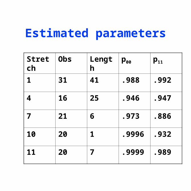
Estimated parameters

Stretch Obs Length p00 p11

1 31 41 .988 .992

4 16 25 .946 .947

7 21 6 .973 .886

10 20 1 .9996 .932

11 20 7 .9999 .989

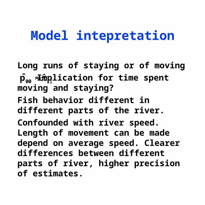
Model intepretation

Long runs of staying or of moving

Implication for time spent moving and staying?

Fish behavior different in different parts of the river.

Confounded with river speed. Length of movement can be made depend on average speed. Clearer differences between different parts of river, higher precision of estimates.

p̂00 ≈p̂11

Tornado model

C. Marzban, M. Drton and P. Guttorp (2003): A Markov chain model of tornadic activity. Monthly Weather Review 131: 2941-2953.

Scientific issue: Tornado prediction

Data: 49 years of daily indicators of occurrence of a tornado in continental US

Varies with time of year

Time-dependent transition probabilities

Tornado alley

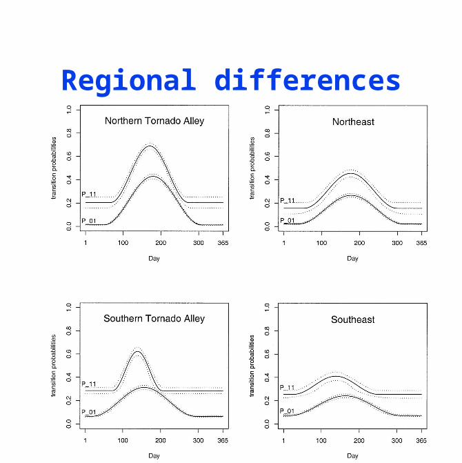
Regional differences

Why is it so?

Frontal systems stay in a region for several days, conducive to tornado activity. So then p11 > p01.

In southern Tornado alley frontal systems cease around mid-May, decreasing p11, but p01 continues to increase for another month due to lots of moisture and weak upper atmosphere systems

SE tornado activity related also to tropical storms, so lasts longer, less pronounced peaks

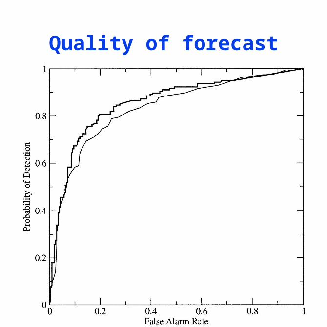
Quality of forecast

Precipitation modeling

J. P. Hughes and P. Guttorp (1994): Incorporating spatial dependence and atmospheric data in a model of precipitation. Journal of Applied Meteorology 33: 1503-1515. IPCC SAR.

Scientific problem: Downscaling climate models to model regional precipitation

A spatial Markov model

Three sites, A, B and C, each observing 0 or 1. Notation: AB = (A=1,B=1,C=0)

Markov model:

Great Plains data1949-1984 (Jan-Feb)

€

P(Xt ≡ (XA,t ,XB,t ,XC,t ) = (i, j,k) | Xt −1 = (l,m,n),...,X1)

= plmn,ijk

Dry A B C AB AC BC ABC

Obs 718 1020 1154 957 866 752 728 657

MC 722 942 1076 1031 789 750 727 655

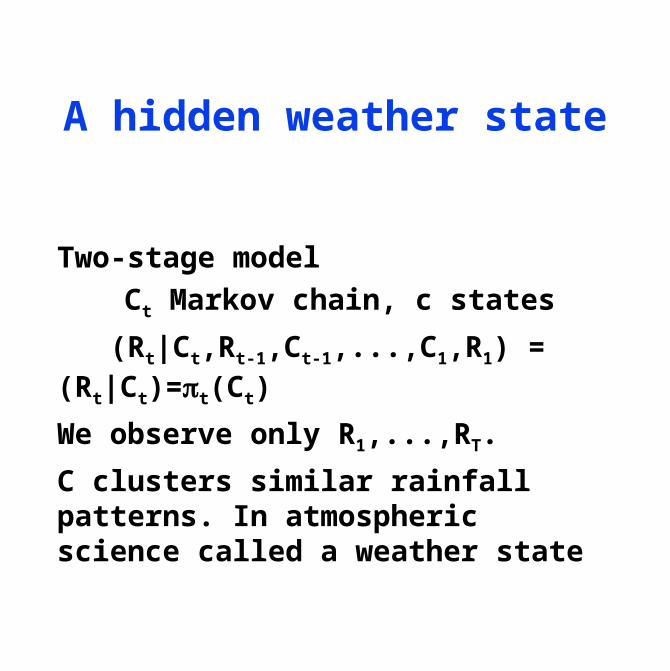
A hidden weather state

Two-stage model

Ct Markov chain, c states

(Rt|Ct,Rt-1,Ct-1,...,C1,R1) = (Rt|Ct)=t(Ct)

We observe only R1,...,RT.

C clusters similar rainfall patterns. In atmospheric science called a weather state

The spatial case

MC: 8 states, 56 parameters

HMM: 2 hidden states (one fairly wet, one fairly dry), 8 parameters, rain conditionally independent at different sites given weather state

Dry A B C AB AC BC ABC

Obs 718 1020 1154 957 866 752 728 657

HMM 725 1019 1153 956 862 749 728 657

MC 722 942 1076 1031 789 750 727 655

Nonstationary transition probabilities

Meteorological conditions may affect transition probabilities

At-1 At

Ct-2 Ct-1 Ct

Rt-2 Rt-1 Rt

€

logpij (t)

1− pij (t)

⎛

⎝ ⎜

⎞

⎠ ⎟ = α ij + βj

TAt

A model for Western Australia rainfall

1978–1987 (1992) winter (May– Oct) daily rainfall at 30 stations

Atmospheric variables in model: E-W gradient in 850 hPa geopotential height, mean sea level pressure, N-S gradient in sea-level pressure

Final model has six weather states

Rain probabilities

Blood production in animals

J. L. Abkowitz, S. N. Catlin, and P. Guttorp (1996): Evidence that hematopoiesis may be a stochastic process in vivo. Nature Medicine 2: 190-197

Scientific problem: Understanding how stem cells for blood production work

Stem cells are not identifiable except by function

Hematopoiesis model

Stem cells Contributing clones

Symmetric division

Asymmetric division

Apoptosis

Specialization

Observations

Exhaustion

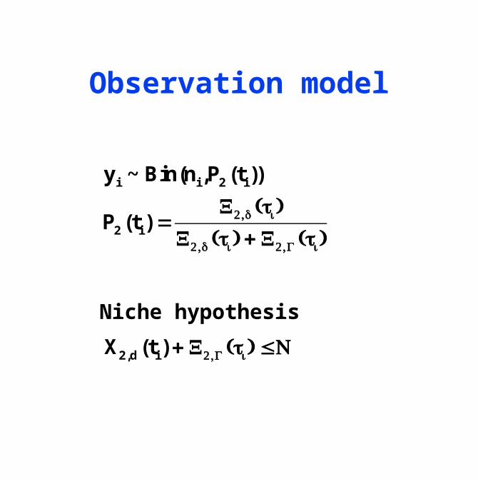
Observation model

yi ~ Bin(ni,P2 (ti ))

P2 (ti ) =X2,d (ti )

X2,d (ti ) + X2,G (ti )

X2,d (ti ) + X2,G (ti ) ≤N

Niche hypothesis

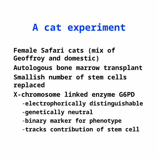
A cat experiment

Female Safari cats (mix of Geoffroy and domestic)

Autologous bone marrow transplant

Smallish number of stem cells replaced

X-chromosome linked enzyme G6PD-electrophorically distinguishable-genetically neutral-binary marker for phenotype-tracks contribution of stem cell

Some data

%dG6PDCat 40004 Cat 40006

Weeks Weeks

Cat 40628 Cat 40665020406080100

0 100200300

020406080100

0 100200300

C a t 4 0 0 0 5

Weeks

Cat 406290204060801000 100200300

020406080100

0 100200300020406080100

0 100200300%dG6PD

020406080100

0 100200300% d G 6 P D

Cat 40004 Cat 40006

Weeks Weeks

Cat 40628 Cat 40665020406080100

0 100200300

020406080100

0 100200300

C a t 4 0 0 0 5

Weeks

Cat 406290204060801000 100200300

020406080100

0 100200300020406080100

0 100200300%dG6PD

020406080100

0 100200300

A Markov chain Monte Carlo approach

Want p(|y)

Marginalize p(,x[0,T]|y)Outer step (parameter update):

Draw from p(|x[0,T],y) Gibbs sampler

Inner step (state update):Draw x[0,T] from p(x[0,T|,y)RJMCMCNon-local updates

State update moves

Deletion of randomly chosen event

Insertion of randomly chosen event

Shuffle: move a randomly chosen event to a new time

Deletion and insertion change state space dimension

Difficulty: if too many events between observation times

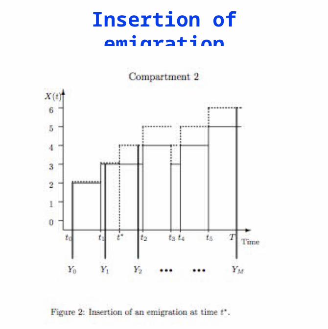
Insertion of emigration

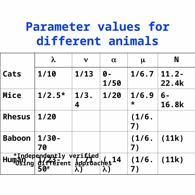
Parameter values for different animals

N

Cats 1/10 1/13 0-1/50 1/6.7 11.2-22.4k

Mice 1/2.5* 1/3.4 1/20 1/6.9* 6-16.8k

Rhesus 1/20 (1/6.7)

Baboon 1/30-70 (1/6.7) (11k)

Human 1/23-50# (.71) (.14) (1/6.7) (11k)

*Independently verified#Using different approaches